femto-PIXAR: a neural network method for reconstruction of femtosecond X-ray free electron laser pulse energy

Abstract

X-ray Free Electron Lasers (X-FELs) operate in a wide range of lasing configurations for a broad variety of scientific applications at ultrafast time-scales such as structural biology, materials science, and atomic and molecular physics. Shot-by-shot characterization of the X-FEL pulses is crucial for analysis of many experiments as well as tuning the X-FEL performance, but an outstanding challenge exist for monochromatic multi-bunch studies, such as those needed for the study of fluctuations in quantum materials. In particular, there is no current method for reliably resolving the pulse intensity profile at sub-picosecond time separation between pulses. Here we show that a physics-based U-net model can reconstruct the individual pulse power profiles on the sub-picoseond pulse separation time. Using experimental data from weak X-FEL pulse pairs, we demonstrate we can learn the pulse characteristics on a shot-by-shot basis when conventional methods fail.

I Introduction

Fluctuations in microscopic systems are directly related to their fundamental excitations – a concept dating back to Einstein’s description of the Brownian motion of pollen particles. This relationship has motivated the need for measuring fluctuations within microscopic systems to directly compare with first-principles theoretical models. However, the spatial and temporal scales of quantum systems far exceed those accessible by classical microscopy, and despite the advances in modern light sources, the energy scales pertinent to these fluctuations remain challenging to probe. One notable exception to this has been in inelastic neutron scattering, where small energy changes of scattered neutrons can be observed, and has led to understanding of dispersion in a myriad of areas, from frustrated magnets and high temperature superconductors, to biological tissue and exotic topological structures, such as skyrmions. However, the reliance of this on large crystals and its limitations with strongly absorbing elements restrict its applicability. The advent of the free electron laser has changed all of this. Its capability to generate femtosecond (fs) laser pulses with extremely high pulse energies at X-ray wavelengths has ushered in a new era of science, with new developments rapidly evolving in many fields [1, 2] including structural biology [3, 4], enzyme catalysis [5], and astrophysics [6, 7]. Furthermore, the development of coherent, two-pulse configurations brings new potential for fluctuation studies within quantum materials at their relevant timescales, i.e. at the meV energy scale and below [8, 9, 10, 11, 12, 13].

Importantly, with X-FELs it is now possible to deliver coherent X-ray pulses at sub-picosecond spacing for experiments, resolving snapshots in structures with sub-Angstrom resolution, and comparing these scattering events to measure fluctuations, but critically, no current method exists to temporally resolve these individual incident pulses at such fine timescales. This highlights the urgent need for reliable characterization of X-FEL laser pulse intensities with femtosecond resolution. Such methods must be robust across various lasing configurations and experimental setups. Notably, X-FELs are highly sensitive to operational parameters which govern the durations, energies, and sequences of X-ray pulses [14, 15]. Compounding this complexity, X-FELs exhibit intrinsic intensity fluctuations, causing shot-to-shot variations in the pulse energy spectrum and photon density [16, 17]. These beam intensity fluctuations from the X-FEL present significant challenges for experiments where accurate characterization of pulse properties, including pulse duration and energy density, is essential to extract meaningful results. These challenges have so far hindered use of this new capability to deliver new science in the observation of fluctuations for understanding properties in materials.

Figure 1: (a) Diagram of the generation and shaping of a single-shot X-ray pulse pair at the LCLS, beginning with the transmission of a single electron bunch through the double-slotted foil. (b) Diagram of the ML training process. (c) Diagram of the ML-based reconstruction of the transient X-ray power profile $P(t)$ from a single-shot lasing-on image.

We address this need by developing a novel self-supervised machine learning (ML) framework called femto-PIXAR: femtosecond Photon Inference of X-ray pulses using AI References, which provides sufficient sensitivity to resolve microjoule-scale pulses with femtosecond pulse separation. We show our approach accurately predicts pulse energies for an experimental dataset, verified against total pulse energy monitors in real X-FEL data, and confirm the predictions match the expected pulse delays. This demonstration will make fluctuation studies possible in the sub-picosecond regime, but will also provide a tool for a wide array of X-FEL experiment in many other fields as well.

II Setup

The experimental setup was designed to produce two coherent X-ray pulses starting from a single, long electron bunch, itself generated from two overlapping injector lasers. The two X-ray pulses were created using a double-slotted V-shaped foil (for time domain control) [18] [19] and hard X-ray self-seeding [20] (for coherence and energy selection). To our knowledge this configuration, described in Fig. 1 a), has never been used before. The experiment was conducted at a photon energy of 8.35 keV (Ni $K$-edge), with slotted-foil pulse separations of $0\,\mathrm{fs}$ (single pulse), $\approx 20\,\mathrm{fs}$, and $\approx 30\,\mathrm{fs}$. Different stages of the electron bunch shaping sequence are labeled $e^{-}_{\text{I}}$, $e^{-}_{\text{II}}$, $e^{-}_{\text{III}}$, $e^{-}_{\text{IV}}$, representing the same electron distribution at different instances as it proceeds in time. A 3 $\mu$m thick aluminum foil with two slots of variable separation from 1 mm to 5 mm is placed in the middle of the dispersive section of the bunch compressor BC2 [18]. At the locations where the electron bunch $e^{-}_{\text{I}}$ passes through the foil the electron emittance is ‘spoiled’ (i.e. increases) due to coulomb scattering. The emittance growth suppresses FEL amplification in the undulator, so that only the electrons $e^{-}_{\text{II}}$ that pass through the slits of the V-shaped foil produce X-ray pulses.

Downstream of the bunch compressor the relative distance between the unspoiled electron distributions $e^{-}_{\text{III}}$ is now in the direction of travel, resulting in an arrival time difference $\Delta t$, that can be changed by shifting the slotted foil. $e^{-}_{\text{IV}}$ passes through the undulator magnets resulting in X-ray lasing. Between the first and second undulator segment a hard X-ray self-seeding scheme is applied (not shown here). Downstream of the undulators, the X-band Transverse deflecting mode CAVity (XTCAV) is employed. [21]. The deflected electron bunch is streaked across the target screen to image the longitudinal distribution, while the X-ray gas-monitor detector (XGMD) [22] measures the total photon pulse energy. The X-rays continue down the beamline to the experimental endstations. This entire process repeats at a 120 Hz repetition rate.

Figure 2: Demonstration of femto-PIXAR reference creation: at the top are dark subtracted XTCAV images for three different slotted foil setups (lasing-on) and a lasing-off sample for the 30 fs delay setup; the second line shows the network’s predicted lasing-off reconstruction; the third line shows the difference image between the measured XTCAV and the reconstructed lasing-off reference; and the last line shows the reconstructed power profiles.

III Data and Methodology

The XTCAV images the longitudinal (time-energy) distribution of the post-lasing electron bunch. By comparison with a lasing-off reference, it is possible to infer the temporal profile of the photon pulse. However, because the lasing-off reference cannot be measured simultaneously, the reference must be inferred from the lasing-on measurement. The “classical” approach has been to record a set of images while suppressing lasing, cluster these images by shape, and then select the most similar cluster for each lasing-on image by comparing the projected electron current [21, 23, 24]. While the classical approach has been demonstrated for various two-pulse modes [19, 25, 14], it struggles for small pulse energies, when shot-to-shot differences between the true lasing-off electron bunch and the selected reference cluster exceed the lasing-induced changes. As a result, when combining seeding with two-pulse modes, the classical method breaks down.

A deep learning method proposed by Ren et al. [26] sidesteps the need for matched lasing-off references by training a neural network (NN) directly to predict power from a lasing-on image; however, the NN relies on accurate simulations for training, and the lack of transverse phase space diagnostics makes this particularly challenging for the complex distributions in the conditions implementing the slotted foil. On the other hand, for the slotted foil setup, only a narrow segment of the beam lases. We can exploit this feature to approximate a reference in the short lasing region by using information in the nearby non-lasing regions. For example, Zeng et al. [27] suggested to use a polynomial regression across the lasing region as a reference. However, the polynomials cannot model the complex phase space of this setup and fail to reproduce the weak lasing pulses (see Fig. 3).

Here, we instead propose an approach using a U-net [28] to generate the corresponding lasing-off reference image. We train the NN using self-supervision, eliminating the need for simulations. Specifically, we mask regions of lasing-off pulses, and train the NN to regenerate those regions. Once trained, the network receives a lasing-on image with masked lasing regions and reconstructs the best lasing-off reference. We then calculate the center of mass (COM) to retrieve the X-ray pulse distribution [24]. The network can also detect the lasing region by identifying areas with the largest reconstruction discrepancy. Our method provides high-fidelity lasing-off references without relying on the accuracy of high-performance computing simulations while retaining interpretability through direct observation of the generated reference.

Figure 3: Correlations with the XGMD for the three different delays using the U-net approach. Both the classical method and polynomial regression show poor correlation between the predicted power-profile integrals and the total XGMD pulse energy especially on the weaker double pulses ( $\approx 20\,\mathrm{fs}$ and $\approx 30\,\mathrm{fs}$ delay).

Figure 1 b) and c) show the core steps. The input of the network are cropped, background subtracted and normalized lasing off images, where all values within two random mask-regions are set to zero (black bars in Fig. 1 b) and c)). The width of an individual mask was chosen to be 16 pixels and the distance range for the two masks was set from 0 pixel to 40 pixel, corresponding to approx. 0 to 38 fs. We then train a U-net to reconstruct the electron phase space of the lasing-off data (Fig. 1 b) ). As the center of mass is the critical value for evaluation, we use a loss that combines the Mean Squared Error of pixel values with the absolute error of the COM. After training, we can mask the lasing regions in a lasing-on data set. As the network is trained only on lasing-off regions of phase space, it will reconstruct the best matching lasing-off electron phase space exactly for a given image (Fig. 1 c). This lasing-off image will also exactly match the original x and y position, so no shifting in the time axis or normalization with the XGMD (as in the classical approach) is necessary.

A crucial step is this process is in determining correct mask positions in lasing-on data. The separation of the two pulses is approximately fixed by the slit separation, but due to shot-to-shot differences in electron bunch energy and compression of the electron bunch, the position of the features relative to the center of mass of the electron bunch is not constant. Our method scans the image to find two locations where input and reconstruction differ most, centering the masks on the maximum signal. We then use the methods from Behrens et. al, marked as $f(a,b)$ in Fig. 1[24] to obtain the power profile using the spectral COM from both images.

IV Results

Fig. 2 shows example reconstructions for the three different configurations and one lasing-off example, all randomly selected from the top 1$\%$ of data with the highest XGMD values (ensuring a clearly visible signal). None of these images were part of the network training process. To demonstrate the efficacy of the proposed method, we benchmark the predicted power and delay against existing diagnostics. First, we compare the integral of the predicted profile with the total energy of both pulses measured by the XGMD, which cannot resolve pulses on the fs scale. In Fig. 3 one can see the correlation of the integral of the power profile with the XGMD for the three different slotted foil configurations. We note that while there is a strong linear correlation between the predicted power and XGMD monitor, there is a disagreement in proportionality. Further experiments are necessary to determine if it is due to either the XGMD or XTCAV calibration, or bias from the method. However, as the typical user experiment usually relies primarily on the relative power between the pulse pairs, this discrepancy does not affect the experimental analysis.

We compare our predictions to two existing state-of-the-art XTCAV analysis methods. In order to evaluate the correlation with the XGMD, in the classical approach (see the previous section), the energy jitter (shift in the y-axis) cannot be compensated for by normalization with the XGMD but must instead be corrected using a scheme that matches the head and tail of the COM profiles for the lasing-on and lasing-off images. We also compare to the polynomial regression method of Zeng et al. [27]. Some example predictions of this method can be found in the supplemental material. Figure 3 compares the XGMD correlation for all three delays, neither of which results in the expected correlation.

Fig. 4 shows the temporal and energy characteristics of the X-ray laser pulses as retrieved by the U-net NN reconstruction scheme. The time assignments of each shot are obtained by fitting the X-ray power trace with two Gaussian functions. For these plots we take only the data where both gaussian curves indicate a signal larger than 15 ${\mu}$J. We find that the predicted time difference between both pulses closely matches the delay given by the slotted foil condition. The temporal separation jitter aligns well with the 9$\%$ jitter observed by Ding et al. [19]. As an additional benchmark we checked the predicted pulse energies for lasing-off data with randomly placed masks and find that 80$\%$ of the data has a deviation from zero of less than 15 $\mu$J, and 99.8$\%$ less than 25 $\mu$J. We also find that the pulse energy difference between the two pulses is centered well around zero for lasing-off-data, indicating that our approach does not introduce a bias in the ratio between the first (left) and the second (right) pulse (see supplemental material).

Figure 4: (a) & (b): Histograms of temporal separation $\Delta t$ between each pulse in time. (c) & (d): Histograms of the integrated energy in each pulse. The insets show averages of the X-ray power profiles, where the relative amplitudes of the pulse 1 (p1) and pulse 2 (p2) are above the dashed 15 muJ threshold.

V Discussions and Summary

In conclusion, femto-PIXAR is a novel X-FEL diagnostic which we demonstrate by reconstructing the X-ray power profiles from weak X-FEL pulses in a non-standard two-pulse, self-seeding configuration. For this configuration, the classical method of XTCAV analysis, which uses a matching algorithm to subtract similar lasing-off shots for the energy loss calculation, fails to reproduce meaningful correlations with the X-ray gas detector. By contrast, our method is able to distinguish the relative amplitude of each X-ray pulse on a shot-to-shot basis which is necessary for X-ray photon fluctuation spectroscopy experiments and other future experiments at X-FEL facilities. Our approach has various benefits, avoiding the need for energy calibration with an external reference and scaling well for high-throughput experiments enabled by next generation X-FEL facilities such as the LCLS-II [29]. As opposed to previous deep-learning work, our approach uses self-supervision with a physics-motivated loss function, avoiding the need for high-fidelity simulations. Our method also reconstructs the full 2D phase space, providing interpretability of the network and giving crucial information about when the network might not be applicable for a specific dataset. Future work will consider extensions to more general XFEL configurations beyond the slotted foil for generation of sub-picosecond-spaced pulses. For example, using diagnostics beyond the XTCAV could enable analysis of configurations with lasing across the full electron bunch [30]. The analysis chain after reconstructing the lasing-off reference can also make use of machine learning, e.g. incorporating spectral measurements to refine the x-ray pulse profile [31].

VI acknowledgments

Use of the Linac Coherent Light Source (LCLS), SLAC National Accelerator Laboratory, is supported by the US Department of Energy, Office of Science, Office of Basic Energy Sciences under Contract No. DE-AC02-76SF00515. The authors acknowledge support from DESY (Hamburg, Germany). This work has in part been funded by the IVF project InternLabs-0011 (HIR3X) J.J.Turner acknowledges support from the U.S. Department of Energy (DOE), Office of Science, Basic Energy Sciences under Award No. DE-SC0022216.

Supplemental Materials

VII A1: Data preparation

The centered XTCAV images have a shape of 240 x 240 pixel. A median dark image is subtracted and they are normalized to have intensities roughly between 0 and 1 before they are used in the network. Before obtaining the power profiles a median filter is used to identify the signal region and set the other regions to zero. This approach is just used to identify the signal region, no median operation is applied to the image.

VIII A2: Network analysis

We used an U-net architecture as described in [28]. The optimizer is RMSprop of pytorch with a weight decay of 1e-8. Out of some manual tries, we picked a learning rate of 5e-7 and a batch size of 2. We found that we get good reconstructions with this parameter set. A more extensive hyper parameter search might provide slightly better reconstructions or faster conversion of the network. However we found that the data preparation like scaling and centering is way more important than the exact hyper parameters. For the loss we used an MSE loss on the reconstruction, combined with an absolute error on the COM. The COM has a relative low weight of 1e-4 as we found that higher weights significantly worsen the reconstruction.
In all our lasing-on datasets we exclude images with weak XGMD signal ($<5\,\mu$J). With this threshold we discarded about 15% of our data, resulting in about $4\times 10^{5}$ samples with approx. $20$ fs difference, about $1.5\times 10^{6}$ samples with approx. $30$ fs difference and $9\times 10^{4}$ with only one pulse. Weak shots (where essentially no lasing occurs) with $E_{\text{GMD}}<5\,\mu$J are included in the lasing-off dataset to get more training data. This results in about 30K lasing-off samples.

IX A3: Classical analysis

For the classical analysis the signal region is identified as described in Appendix A, and then divided into 120 slices so that all lasing-on and lasing-off data has the same length in slices and lasing-on and lasing-off data can be compared directly. HierarchicalClustering (sklearn.cluster.AgglomerativeClustering) with euclidean distance is used to cluster the current profiles into 500 groups. Normally, a few hundred lasing-offs are used to build a reference set, but to have a fairer comparison all lasing-off images that are used in the training of the network are provided to the algorithm. The COM profile of these groups are averaged and used as reference.

X A3: Implementation of polynomial regression method

For the polynomial regression we used an algorithm described in [32]. Zeng et al. [27] uses a 13 dimensional polynomial, we find that our algorithm does not converge in this case. In Fig. A1 we show one example of the regression method with increasing polynomial degrees. In our benchmark we use the highest degree where the algorithm converges, with a maximum of 13. In Fig. A2 we show resulting regressions for ten different samples. We found that the predictions have a better correlation with the XGMD if we ignore the (obvious wrong) parts of the predicted profile that are negative.

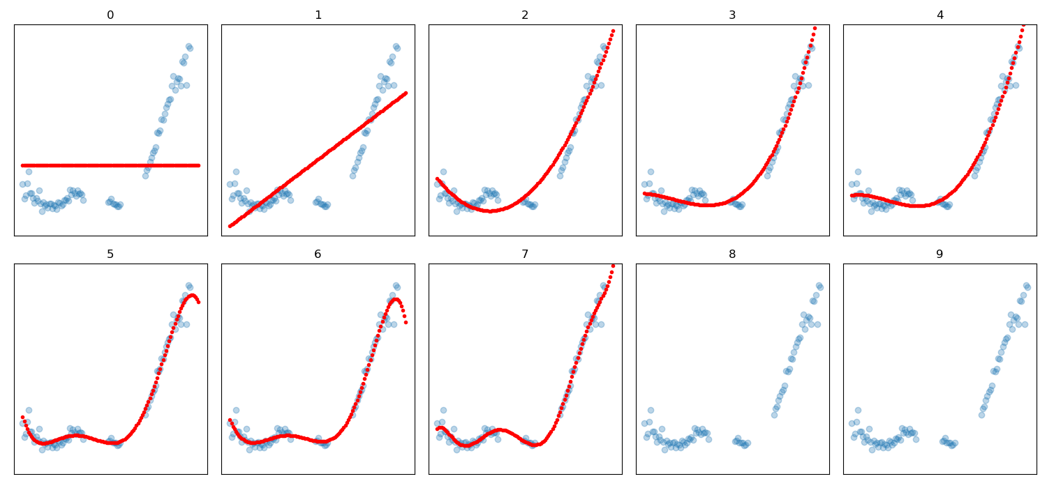
Figure A1: The blue dots mark the COM for one sample. The COM within the mask region is reconstructed with increasing polynomial degrees. For a degree higher larger seven, it does not converge.

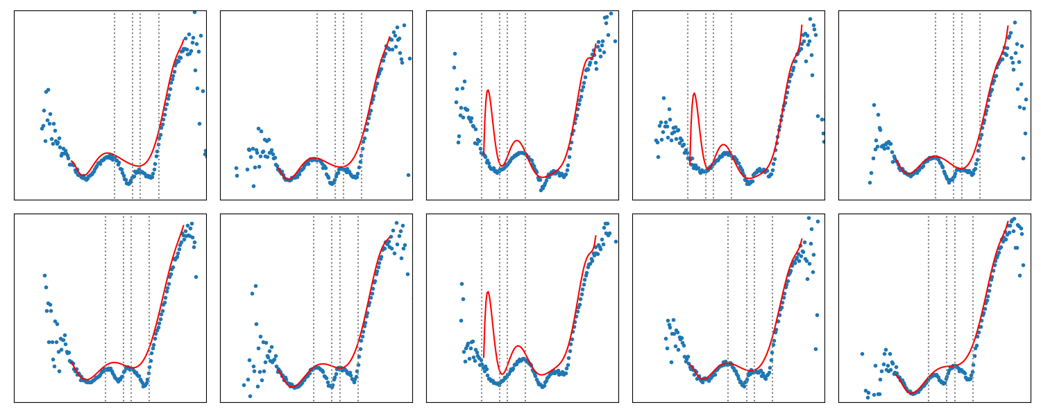
Figure A2: Resulting regression profiles for ten different samples. In case c) and h) the regression predicts additional maxima. In all cases it does not follow the drop completely. Therefore this approach produces a higher spread and an offset compared to the XGMD benchmark.

XI A4: Residual error benchmark

An additional method to benchmark our method is to evaluate the generated power profiles for data where no lasing process took place. Ideally, for this setup, the integral of the power profiles would be zero. Fig. A3 shows a histogram of the resulting energies of 4600 non-lasing data points. We used 460 lasing-off samples that were not part of the network training and used each of them 10 times with randomly set masks. 80$\%$ of the data has a deviation from zero of less than 15 $\mu$J, 99.8 $\%$ less than 25 $\mu$J. As we are interested in the pulse ratio between the two peaks it is important that not one of the pulses is systematically under and the other over estimated. We check this on the right side of Fig. A3 and see that the pulse energy difference between the two pulses is centered well around zero. This indicates, that, for this dataset, not one pulse is overestimated over the other.

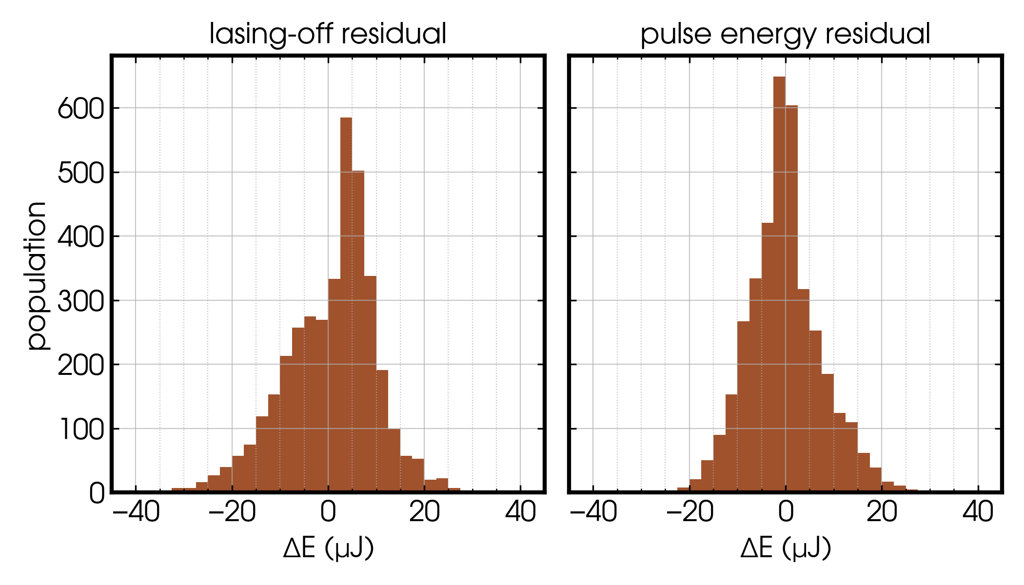
Figure A3: Histogram of the deviation from zero of the derived sum energy of lasing-off power profile predictions. On the left you can see the sum of the integral of the Gaussian fits of both power profiles, on the right the difference between the first and the second peak. The sum is biased towards the positive side as the starting values for the Gaussian fits are positive.

XII A5: Time distribution extracted from reconstructed profiles

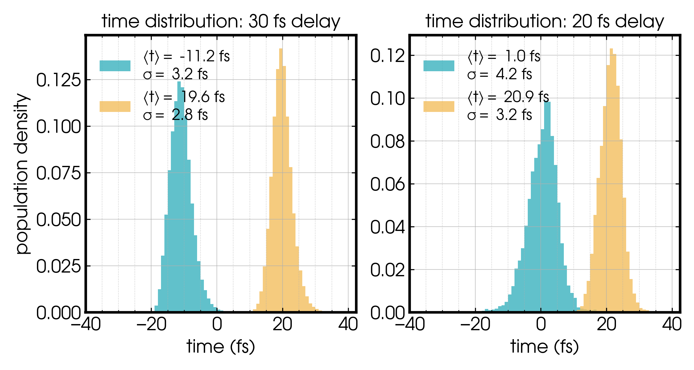
Figure A4: Distribution of pulse arrival times from both two-pulse setups. $t=0$ is defined by the center of mass of the XTCAV spectrograph.

Using a double-Gaussian fit over the reconstructed transient X-ray power profiles, we are able to determine the arrival times of the two pulses at the XTCAV target. The time axis in A4 is centered with respect to the COM of the spectrograph in the temporal domain. The reconstructed pulses obtained by the Gaussian fits produce bimodal time distributions that match the X-FEL setups, with average time jitter of 3.3 fs.

References

- Bostedt et al. [2016] C. Bostedt, S. Boutet, D. M. Fritz, Z. Huang, H. J. Lee, H. T. Lemke, A. Robert, W. F. Schlotter, J. J. Turner, and G. J. Williams, Linac coherent light source: The first five years, Rev. Mod. Phys. 88, 015007 (2016).
- Rossbach et al. [2019] J. Rossbach, J. R. Schneider, and W. Wurth, 10 years of pioneering x-ray science at the free-electron laser flash at desy, Physics reports 808, 1 (2019).
- Boutet et al. [2012] S. Boutet, L. Lomb, G. J. Williams, T. R. Barends, A. Aquila, R. B. Doak, U. Weierstall, D. P. DePonte, J. Steinbrener, R. L. Shoeman, et al., High-resolution protein structure determination by serial femtosecond crystallography, Science 337, 362 (2012).
- Chapman et al. [2011] H. N. Chapman, P. Fromme, A. Barty, T. A. White, R. A. Kirian, A. Aquila, M. S. Hunter, J. Schulz, D. P. DePonte, U. Weierstall, et al., Femtosecond x-ray protein nanocrystallography, Nature 470, 73 (2011).
- Rose et al. [2021] S. L. Rose, S. V. Antonyuk, D. Sasaki, K. Yamashita, K. Hirata, G. Ueno, H. Ago, R. R. Eady, T. Tosha, M. Yamamoto, et al., An unprecedented insight into the catalytic mechanism of copper nitrite reductase from atomic-resolution and damage-free structures, Science advances 7, eabd8523 (2021).
- Bernitt et al. [2012] S. Bernitt, G. V. Brown, J. K. Rudolph, R. Steinbrugge, A. Graf, M. Leutenegger, S. W. Epp, S. Eberle, K. Kubicek, V. Mackel, et al., An unexpectedly low oscillator strength as the origin of the fe xvii emission problem, Nature 492, 225 (2012).
- Vinko et al. [2012] S. M. Vinko, O. Ciricosta, B. I. Cho, K. Engelhorn, H. K. Chung, C. R. Brown, T. Burian, J. Chalupsky, R. W. Falcone, C. Graves, et al., Creation and diagnosis of a solid-density plasma with an x-ray free-electron laser, Nature 482, 59 (2012).
- Sun et al. [2020] Y. Sun, M. Dunne, P. Fuoss, A. Robert, D. Zhu, T. Osaka, M. Yabashi, and M. Sutton, Realizing split-pulse x-ray photon correlation spectroscopy to measure ultrafast dynamics in complex matter, Physical Review Research 2, 023099 (2020).
- Gutt et al. [2008] C. Gutt, L.-M. Stadler, A. Duri, T. Autenrieth, O. Leupold, Y. Chushkin, and G. Grübel, Measuring temporal speckle correlations at ultrafast x-ray sources, Optics express 17, 55 (2008).
- Plumley et al. [2024] R. Plumley, S. Chitturi, C. Peng, T. Assefa, N. Burdet, L. Shen, Z. Chen, A. Reid, G. Dakovski, M. Seaberg, et al., On ultrafast x-ray scattering methods for magnetism, Advances in Physics: X 9, 2423935 (2024).
- Seaberg et al. [2017] M. Seaberg, B. Holladay, J. Lee, M. Sikorski, A. Reid, S. Montoya, G. Dakovski, J. Koralek, G. Coslovich, S. Moeller, et al., Nanosecond x-ray photon correlation spectroscopy on magnetic skyrmions, Physical Review Letters 119, 067403 (2017).
- Seaberg et al. [2021] M. Seaberg, B. Holladay, S. Montoya, X. Zheng, J. Lee, A. Reid, J. Koralek, L. Shen, V. Esposito, G. Coslovich, et al., Spontaneous fluctuations in a magnetic fe/gd skyrmion lattice, Physical Review Research 3, 033249 (2021).
- Roseker et al. [2018] W. Roseker, S. Hruszkewycz, F. Lehmkühler, M. Walther, H. Schulte-Schrepping, S. Lee, T. Osaka, L. Strüder, R. Hartmann, M. Sikorski, et al., Towards ultrafast dynamics with split-pulse x-ray photon correlation spectroscopy at free electron laser sources, Nature communications 9, 1704 (2018).
- Decker et al. [2022a] F.-J. Decker, K. L. Bane, W. Colocho, S. Gilevich, A. Marinelli, J. C. Sheppard, J. L. Turner, J. J. Turner, S. L. Vetter, A. Halavanau, et al., Tunable x-ray free electron laser multi-pulses with nanosecond separation, Scientific Reports 12, 3253 (2022a).
- Decker et al. [2022b] F.-J. Decker, W. Colocho, A. Halavanau, A. Lutman, J. MacArthur, G. Marcus, R. Margraf, J. Sheppard, J. Turner, and S. Vetter, Two and Multiple Bunches with the LCLS Copper Linac, Tech. Rep. (SLAC National Accelerator Lab., Menlo Park, CA (United States), 2022).
- Bonifacio et al. [1994] R. Bonifacio, L. De Salvo, P. Pierini, N. Piovella, and C. Pellegrini, Spectrum, temporal structure, and fluctuations in a high-gain free-electron laser starting from noise, Physical review letters 73, 70 (1994).
- Sun et al. [2018] Y. Sun, F.-J. Decker, J. Turner, S. Song, A. Robert, and D. Zhu, Pulse intensity characterization of the lcls nanosecond double-bunch mode of operation, Journal of synchrotron radiation 25, 642 (2018).
- Emma et al. [2004] P. Emma, M. Borland, and Z. Huang, Attosecond x-ray pulses in the lcls using the slotted foil method, in Proc. FEL’04. Trieste, Italy (JACoW Publishing, pp. 333–338., 2004).
- Ding et al. [2015] Y. Ding, C. Behrens, R. Coffee, F.-J. Decker, P. Emma, C. Field, W. Helml, Z. Huang, P. Krejcik, J. Krzywinski, H. Loos, A. Lutman, A. Marinelli, T. J. Maxwell, and J. Turner, Generating femtosecond x-ray pulses using an emittance-spoiling foil in free-electron lasers, Applied Physics Letters 107, 191104 (2015).
- Amann et al. [2012] J. Amann, W. Berg, V. Blank, F.-J. Decker, Y. Ding, P. Emma, Y. Feng, J. Frisch, D. Fritz, J. Hastings, Z. Huang, J. Krzywinski, R. Lindberg, H. Loos, A. Lutman, H.-D. Nuhn, D. Ratner, J. Rzepiela, D. Shu, Y. Shvyd’ko, S. Spampinati, S. Stoupin, S. Terentyev, E. Trakhtenberg, D. Walz, J. Welch, J. Wu, A. Zholents, and D. Zhu, Demonstration of self-seeding in a hard-x-ray free-electron laser, Nature Photonics 6, 693 (2012).
- Ding et al. [2011] Y. Ding, C. Behrens, P. Emma, J. Frisch, Z. Huang, H. Loos, P. Krejcik, and M.-H. Wang, Femtosecond x-ray pulse temporal characterization in free-electron lasers using a transverse deflector, Physical Review Special Topics - Accelerators and Beams 14, 120701 (2011).
- Sorokin et al. [2019] A. A. Sorokin, Y. Bican, S. Bonfigt, M. Brachmanski, M. Braune, U. F. Jastrow, A. Gottwald, H. Kaser, M. Richter, and K. Tiedtke, An X-ray gas monitor for free-electron lasers, Journal of Synchrotron Radiation 26, 1092 (2019).
- Maxwell et al. [2014] T. J. Maxwell, C. Behrens, Y. Ding, Z. Huang, P. Krejcik, A. Marinelli, L. Piccoli, and D. Ratner, Femtosecond-scale x-ray FEL diagnostics with the LCLS x-band transverse deflector, in SPIE Proceedings, edited by S. P. Hau-Riege, S. P. Moeller, and M. Yabashi (SPIE, 2014).
- Behrens et al. [2014] C. Behrens, F.-J. Decker, Y. Ding, V. A. Dolgashev, J. Frisch, Z. Huang, P. Krejcik, H. Loos, A. Lutman, T. J. Maxwell, J. Turner, J. Wang, M.-H. Wang, J. Welch, and J. Wu, Few-femtosecond time-resolved measurements of x-ray free-electron lasers, Nature Communications 5, 10.1038/ncomms4762 (2014).
- Marinelli et al. [2016] A. Marinelli, R. Coffee, F.-J. Decker, Y. Ding, R. Field, S. Gilevich, Z. Huang, D. Kharakh, H. Loos, A. Lutman, T. Maxwell, J. Turner, and S. Vetter, Twin-bunch two-colour fel at lcls, Proceedings of the 7th Int. Particle Accelerator Conf. IPAC2016, Korea (2016).
- Ren et al. [2020] X. Ren, A. Edelen, A. Lutman, G. Marcus, T. Maxwell, and D. Ratner, Temporal power reconstruction for an x-ray free-electron laser using convolutional neural networks, Physical Review Accelerators and Beams 23, 040701 (2020).
- Zeng et al. [2022] L. Zeng, C. Feng, D. Gu, X. Wang, K. Zhang, B. Liu, and Z. Zhao, Online single-shot characterization of ultrafast pulses from high-gain free-electron lasers, Fundamental Research 2, 929 (2022).
- Ronneberger et al. [2015] O. Ronneberger, P.Fischer, and T. Brox, U-net: Convolutional networks for biomedical image segmentation, in Medical Image Computing and Computer-Assisted Intervention (MICCAI), LNCS, Vol. 9351 (Springer, 2015) pp. 234–241, (available on arXiv:1505.04597).
- Galayda [2018] J. N. Galayda, The LCLS-II: A high power upgrade to the LCLS, Tech. Rep. (SLAC National Accelerator Lab., Menlo Park, CA (United States), 2018).
- Sanchez-Gonzalez et al. [2017] A. Sanchez-Gonzalez, P. Micaelli, C. Olivier, T. Barillot, M. Ilchen, A. Lutman, A. Marinelli, T. Maxwell, A. Achner, M. Agåker, et al., Accurate prediction of x-ray pulse properties from a free-electron laser using machine learning, Nature communications 8, 15461 (2017).
- Ratner et al. [2021] D. Ratner, F. Christie, J. Cryan, A. Edelen, A. Lutman, and X. Zhang, Recovering the phase and amplitude of x-ray fel pulses using neural networks and differentiable models, Optics express 29, 20336 (2021).
- Marholm [2022] S. Marholm, sigvaldm/localreg: Multivariate rbf output (2022).