Finding Influential Cores via Normalized Ricci Flows in Directed and Undirected Hypergraphs with Applications
Abstract
Many biological and social systems are naturally represented as edge-weighted directed or undirected hypergraphs since they exhibit group interactions involving three or more system units as opposed to pairwise interactions that can be incorporated in graph-theoretic representations. However, finding influential cores in hypergraphs is still not as extensively studied as their graph-theoretic counter-parts. To this end, we develop and implement a hypergraph-curvature guided discrete time diffusion process with suitable topological surgeries and edge-weight re-normalization procedures for both undirected and directed weighted hypergraphs to find influential cores. We successfully apply our framework for directed hypergraphs to seven metabolic hypergraphs and our framework for undirected hypergraphs to two social (co-authorship) hypergraphs to find influential cores, thereby demonstrating the practical feasibility of our approach. In addition, we prove a theorem showing that a certain edge weight re-normalization procedure in a prior research work for Ricci flows for edge-weighted graphs has the undesirable outcome of modifying the edge-weights to negative numbers, thereby rendering the procedure impossible to use. To the best of our knowledge, this seems to be one of the first articles that formulates algorithmic approaches for finding core(s) of (weighted or unweighted) directed hypergraphs.
I Introduction
Useful insights for many complex systems are often obtained by representing them as graphs and analyzing them using graph-theoretic and combinatorial tools [1, 2, 3]. Such graphs may vary in diversity from simple undirected graphs to edge-labeled directed graphs. In such graphs, nodes represent the basic units of the system (e.g., system variables) and edges represent relationships (e.g., correlations) between pairs of such basic units. Once such graphs are constructed, they can be analyzed using graph-theoretic measures such as degree-based measures (e.g., degree distributions), connectivity-based measures (e.g., clustering coefficients), geodesic-based measures (e.g., betweenness centralities) and other more novel network measures such as in [4, 5, 6, 7] to give meaningful insights into the properties and the dynamics of the system. However, many real-world systems exhibit group (i.e., higher order) interactions involving three or more system units [8, 9, 10]. One way to handle these higher order interactions is to encode them by a suitable combination of pairwise interactions and then simply use the existing graph-theoretic tools (e.g., see [11, 12]). While such approaches have been successful in the context of many real-world networks, they obviously do not encode the higher-order interactions in their full generalities. A more direct approach would be to use directed or undirected hypergraphs to encode these interactions, and this is the approach we follow in this article. Although the theory of hypergraphs has been considerably developed during the last few decades (e.g., see [13]), applications of hypergraphs to real-world networks face their own challenges. Sometimes it is not clear how to generalize a concept from graphs to hypergraphs such that it best serves its purpose in the corresponding application, and some computationally tractable graph-theoretic algorithms may become intractable when generalized to hypergraphs (e.g., the maximum matching problem for graphs is polynomial-time solvable whereas the -dimensional matching problem for hypergraphs is -complete [14]).
Suitable notions of curvatures are natural measures of shapes of higher dimensional objects in mainstream physics and mathematics [15, 16]. There have been several attempts to extend these curvature measures to graphs and hypergraphs. Two major notions of curvatures of graphs can be obtained via extending Forman’s discretization [17] of Ricci curvature for (polyhedral or CW) complexes to undirected graphs (the “Forman-Ricci curvature”) [18, 19, 20, 21, 22, 23] and via Ollivier’s discretization of manifold Ricci curvature to undirected edge-weighted graphs (the “Ollivier-Ricci curvature”) [24, 25, 26, 27]. Both Ollivier-Ricci curvature and Forman-Ricci curvature assign a number to each edge of the given graph, but the numbers are calculated in very different ways since they capture different metric properties of a Riemannian manifold; some comparative analysis of these two measures can be found in [23, 22]. Recently, the Ollivier-Ricci curvature and the Forman-Ricci curvature measures have been generalized in a few ways to unweighted directed and undirected hypergraphs [28, 29, 30, 31, 32].
A curvature-guided diffusion process called Ricci flow, along with “topological surgery” procedures to avoid topological singularities, was originally introduced in the context of a Riemannian manifold by Hamilton [33] to provide a continuous change of the metric of the manifold to provide a continuous transformation (homeomorphism) of one manifold to another manifold. One of the most ground-breaking application of this technique was done by Perelman [34] to solve the Poincaré conjecture, which asserts that any three-dimensional manifold that is closed, connected, and has a trivial fundamental group is homeomorphic to the three-dimensional sphere. In the context of a weighted undirected graphs, these techniques were extended in papers such as [35, 36, 37, 38, 20, 39, 40] to iteratively and synchronously change the weights of the edges of the graph. Motivated by the fact that connected sum decomposition can be detected by the geometric Ricci flows in manifolds, these techniques were then used to find communities or modules mostly in the context of undirected social graphs. To prevent lack of convergence of graph Ricci flows within reasonable time, edge-weight re-normalization methods after every iteration were suggested and investigated in [37].
In this article we devise a computational framework to detect influential cores in both undirected and directed weighted hypergraphs by formulating and using a hypergraph-curvature guided discrete time diffusion process with suitable topological surgeries and edge-weight re-normalization procedures. We demonstrate the practical feasibility of our approach by successfully applying our computational framework for directed hypergraphs to seven metabolic hypergraphs and our computational framework for undirected hypergraphs to two social (co-authorship) hypergraphs to find influential cores. In addition, we prove a theorem showing that a certain edge weight re-normalization procedure in [37] for Ricci flows for edge-weighted graphs has an undesirable outcome of modifying the edge-weights to negative numbers, thereby rendering the procedure impossible to use.
Motivation for finding core(s) of a complex system
Broadly speaking, the core of a complex system (also studied under the name “cohesive subgraph” in the network science literature [41]) is a smaller sub-system that contributes significantly to the functioning of the overall system, and thus focussing the analysis of the smaller sub-system, which could be easier than analyzing the system as a whole, may reveal important characteristics of the overall system. For example, in the context of brain graphs, identifications of core(s) of the graph where neurons strongly interact with each other provide effective characterizations of these graph topologies; such cores are very important for various brain functions and cognition [42]. As another example, cores in attributed social networks can be directly utilised for a recommendation system [41].
For systems represented by undirected graphs, prior research works have used various definitions of what actually constitutes a core, such as via modularity [43], via rich clubs [44], or using information-theoretic ideas [45].
Our definition for cores of hypergraphs requires sufficient connectivity and cohesiveness, nontrivial size, and a large centrality, evidenced by a large loss of short paths in the network when the core is removed. The specific definition and constraints are given in Section II.3. The specific usefulness of finding cores for metabolic (directed) hypergraphs and for co-authorship (undirected) hypergraphs are discussed in Section III.5.1 and in Section III.5.2, respectively. To the best of our knowledge, this seems to be one of the first articles that formulates algorithmic approaches for finding core(s) of (weighted or unweighted) directed hypergraphs. Note that since graphs are special cases of hypergraphs, our methodologies are also applicable to graphs; however, in this article our focus is on hypergraphs that are not graphs.
Finding cores vs. modular decomposition
Note that finding a core of a system is different than the modular decomposition of graphs that has been extensively studied in the network science literature [46, 47, 48, 49, 50]: the overall goal of graph decomposition (partitioning) into modules (also called communities or clusters) is to partition the entire node set into modules and requires the optimization of a joint fitness function of these modules to evaluate the quality of the decomposition. In particular, the centrality parameters (quantifying loss of short paths when removing the core, see Section II.3) are not relevant for typical modular decomposition applications and the size constraints are unimportant if the joint fitness function is satisfactory (e.g., papers such as [49] show that a good approximation to Newman’s modularity value may be obtained even though the corresponding modules will not satisfy our size constraints).
I.1 Basic Definitions and Notations
A weighted directed hypergraph consists of a node set , a set of (directed) hyperedges and a hyperedge-weight function . A directed hyperedge is an ordered pair where is the tail, is the head and ; for convenience we will also denote the hyperedge by . For a node , the in-degree is the number of “incoming” hyperedges, i.e., the number of hyperedges such that , and the out-degree is the number of “outgoing” hyperedges, i.e., the number of hyperedges such that . A (directed) path from node to node is an alternating sequence of distinct nodes and directed hyperedges such that and for each ; the length of the path is . We will denote by the minimum length of any path from to ; note that need not be same as . A directed hypergraph is weakly connected provided for every pair of nodes and there is either a path from to or a path from to . We assume from now onwards that our original (input) directed hypergraph is weakly connected.
A weighted undirected hypergraph consists of a node set , a set of (undirected) hyperedges and a hyperedge-weight function . A (undirected) hyperedge is a subset of nodes where . For a node , the degree is the number of the number of hyperedges such that . An (undirected) path between nodes and is an alternating sequence of distinct nodes and undirected hyperedges such that for each ; the length of the path is . We will denote by the distance (i.e., minimum length of any path) between and . A undirected hypergraph is connected provided for every pair of nodes there is a path between them. We assume from now onwards that our original (input) undirected hypergraph is connected.
I.2 Discussions on Prior Relevant Research
There are some prior published articles that deal with finding cores or core-like structures for undirected hypergraphs, mostly for unweighted undirected hypergraphs [51, 52, 53, 54, 55, 56, 57, 58, 59, 60] but some also on weighted undirected hypergraphs [61]. However, there seem to be very few peer-reviewed prior articles dealing with finding cores for directed (and more so for weighted directed) hypergraphs where cores are defined in the same sense as used in this article; the authors themselves were unable to get any relevant peer-reviewed prior works via google search. For example, the articles by Pretolani [62] and by Volpentesta [63] investigate intriguing but different concepts that refer to sub-structures in unweighted directed hypergraphs based on hyperpaths. Note that although for graphs replacing an undirected edge by two directed edges make the core finding problem for undirected graphs solvable from the core finding problem for directed graphs, a similar trick cannot directly be used for hypergraphs since the head or tail may contain more than one node (i.e., a core finding algorithm for directed hypergraphs does not readily translate to an algorithm for finding cores in undirected hypergraphs). A strength of our framework is that we have a single overall algorithmic method (albeit with different calculations of certain quantities) that can be adopted for both directed and undirected hypergraphs.
Most of the prior works on finding cores for undirected unweighted hypergraphs involve iteratively identifying a set of nodes such that the degree of every node in the set is at least for a given . We go deeper than these prior works by defining the centrality quality parameters of the core as stated via Equations (12) and (13). These centrality quality parameters, which are combinatorial analogs of the information loss quantifications used in prior research works such as [45], are significant in real-world applications to biological and social networks, as mentioned in prior publications such as [64] in the context of undirected unweighted graphs (e.g., see Figure 5 for biological networks and Figures 7–8 for social networks in [64] with associated texts), and are closely related to the concept of structural holes [65] in social networks.
II Methods and Materials
II.1 Definition of Curvatures of Weighted Hypergraphs
Curvatures of weighted hypergraphs are defined in somewhat different ways depending on whether the hypergraph is directed or undirected. However, both definitions use a common paradigm of Emd (Earth Mover’s Distance, also known as the transportation distance, the Wasserstein distance or the Monge-Kantorovich-Rubinstein distance [66, 67, 68, 69]) defined on the hypergraph in the following manner based on the notations and terminologies in [70]. Let be a directed or undirected hypergraph. Suppose that we have two probability distributions and over the set of nodes , i.e., two real numbers for every node with . We can think of as the total amount of “earth” (dirt) at node that need to be moved to other nodes, and as the maximum total amount of earth node can store. The cost of transporting one unit of earth from node to node is , and the goal is to move all units of earth (determined by ) while simultaneously satisfying all storage requirements (dictated by ) and minimizing the total transportation cost. Letting the real variable denote the amount of shipment from node to node in an optimal solution, Emd for the two probability distributions and on is the linear programming () problem shown in Fig. 1 which can be solved in polynomial time. We will use the notation Emd to denote the value of the objective function in an optimal solution of the in Fig. 1.
| variables: for every pair of nodes | ||
|---|---|---|
| minimize | (* minimize total transportation cost *) | |
| subject to | ||
| for each | (* ship from as much as it has *) | |
| for each | (* ship to as much as it can store *) | |
| for each | ||
Given a hypergraph and an edge of , the curvature value of is then computed as follows:
-
Fix appropriate distributions for and .
-
Use a formula for Ricci curvature of the hyperedge The formula is different depending on whether the hypergraph is directed or undirected, and shown below:
-
For directed hypergraphs, the Ricci curvature of the hyperedge is calculated as:
(1) An informal intuitive understanding of the connection of Emd to Ricci curvature in the above formula, as explained in prior research works such as [24] in the context of graphs, is as follows. The Ricci curvature at a point in a smooth Riemannian manifold can be thought of transporting a small ball centered at along that direction and measuring the “distortion” of that ball. In (1) the role of the direction is captured by the hyperedge , the roles of the balls at the two nodes are played by the distributions and , and the role of the distortion due to transportation is captured by the Emd measure.
-
For undirected hypergraphs, the Ricci curvature of the hyperedge is calculated as:
(2) The calculation for the curvature averages out weighted-lazy random walk probabilities over all pairs of distinct nodes in . There is one special case not covered by the above definition but may occur in our undirected co-authorship hypergraphs: namely when for some node corresponding to a paper written by just one author. For this case we treat the hyperedge as a self-loop from to giving an Emd value of zero.
-
The exact calculations of and are somewhat different depending on whether the hypergraph is directed or undirected, and this is described in next two sections. Let be the weighted (directed or undirected) hypergraph, and be the hyperedge considered.
II.1.1 Calculations of and for a Weighted Directed Hypergraph
The distributions and are determined by the nodes in and , respectively. is determined in the following manner by adopting the calculations in [29]:
-
Initially, for all . In our subsequent steps, we will add to these values as appropriate.
-
We divide the total probability equally among the nodes in , thus “allocating” a value of to each node in question.
-
For every node with , we add to .
-
For every node with , we perform the following:
-
We divide the probability equally among the hyperedges such that , thus “allocating” a value of to each hyperedge in question.
-
For each such hyperedge such that , we divide the allocated value equally among the nodes in and add these values to the probabilities of these nodes. In other words, for every node we add to .
-
Note that the final probability for each node is calculated by summing all the contributions from each bullet point. In closed form, is given by:
where is the Kronecker delta function, i.e.,
is determined in a symmetric manner. The details are provided in the appendix for the sake of completeness.
II.1.2 Calculations of and for an Undirected Hypergraph
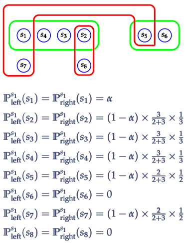
For this case, for all since the hypergraph is undirected. Let be a parameter that encodes the “laziness” of the random walk. Then, is determined in the following manner by adopting the calculations in [30] (see Fig. 2 for an illustration):
-
Initially, and for all . In our subsequent steps, we will add to these values as appropriate.
-
We divide and allocate the remaining total probability among all the hyperedges that contain proportionally to the cardinality of these hyperedges excluding the node , i.e., a hyperedge such that gets . Then, we divide the allocated value equally among the nodes in excluding and add these values to the probabilities of these nodes. In other words, for every node such that we add to .
In closed form, is given by:
The parameter was used in the context of Ricci flows on undirected graphs by Ni et al. [35], and by Lai et al. [37]. These works suggested using a non-zero value for , but the exact choice of was left to the specific application in question. Thus, we decided to use a non-zero value of and found that a value of works best in our applications.
II.2 Ricci Flow, Weight-renormalization, Topological Surgery and Flow Convergence for Weighted Hypergraphs
Before proceeding with the technical descriptions, we first provide a brief informal intuition behind the proposed approach. The curvature values of the hyperedges provide a (positive or negative) value to each hyperedge of the hypergraph. The Ricci flow is an iterative process that produces a sequence of hypergraphs, where each iteration of the Ricci flow process dynamically alters the weights of hyperedges based on their current weights and curvature values. On average, these weight alterations tend to increase the weights of the hyperedges connecting the core(s) to the rest of the hypergraph while decreasing the weights of those hyperedges within the core(s). The weight re-normalization procedure after every iteration ensures that the weights of the hyperedges do not increase in an unbounded manner and instead eventually converge to some “steady-state” values. The goal of the topological surgery procedure performed once in a few iterations is to remove the hyperedges connecting the core(s) to the rest of the hypergraph so that at the end of our Ricci flow process, when the hyperedge weights have converged to some stable values, we can recover the core(s) from the connected components of the hypergraph. This process of topological surgeries and hyperedge weight updates via Ricci flows is somewhat analogous to the Newman-Girvan’s algorithm [71] which, in the context of undirected graphs, iteratively removes edges of high betweenness centrality and recomputes the edge betweenness centrality.
We now present the precise technical descriptions of these concepts. Let is the discrete iteration index, and let denote the sequence of hypergraphs produced by the Ricci flow with being equal to the original (starting) hypergraph . The Ricci flow equation (without topological surgeries and hyperedge-weight renormalization) is as follows [35, 36, 37]:
| (3) |
where is the curvature value based on the edge-weights . Note that if for some value then stays zero for all based on (3), so we may simply remove such edges from all with . Also note that for all since for all .
Unfortunately, as observed in papers such as [37], there are problematic aspects to the Ricci flow equation in (3). In particular, in applications such as in this article, we would like the iterations to eventually converge (within a reasonable time), but it can be easily seen that there exists hypergraphs for which the hyperedge weights may keep on increasing in successive iterations. As a remedy for graphs only, Lai, Bai and Lin [37] proposed changing (3) to (4) as shown below such that the Ricci flow is “normalized” in the sense that the sum of edge weights of the graph remain the same and therefore edge weights cannot become arbitrarily large:
| (4) |
In the above equation, is a constant (called “step size” in [37]). Unfortunately, as we will prove in Theorem in Section III.3, there are infinitely many graphs for which will become negative thus rendering the iterative process in (4) impossible to execute beyond the first step. Instead, in our algorithm we perform hyperedge-weight re-normalization by applying a sigmoidal function to hyperedge weights to ensure that all hyperedge weights do not exceed , i.e., for we replace by . In the sequel, unless explicitly mentioned otherwise, when we refer to weight for we refer to the weight after re-normalization.
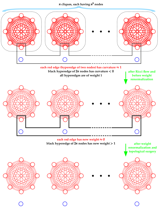
Unfortunately, there is no closed-form analytical solution of Equation (3) yet and it is not even clear if such a solution is possible. Here we introduce our topological surgery operation, and provide an informal intuition behind our approach of finding cores by using Ricci flows with topological surgery. Note that since all hyperedge weights are non-negative at all times, Equation (3) shows that if and if , i.e., each iteration of the Ricci flow process dynamically alters the weights of hyperedges based on their curvature values, increasing the weights of those with negative curvature while decreasing the weights of those with positive curvature. Using the observation in [36] that states (quoted verbatim) “positively curved edges are well connected in the sense that none of them are essential for the proper transport operation”, which is also supported by research works such as [35, 36] on graphs, it follows that this effect should on an average lead to pairs of nodes within a core being connected by hyperedges with a smaller weight whereas pairs of nodes outside cores being connected by hyperedges with a larger weight. Consequently, we can use the following “topological surgery” method to isolate the core(s) from the remaining parts of the hypergraph: remove hyperedges with substantial weights following every several iterations of the Ricci flow. This strategic manipulation enhances the clarity of core structures within the network. Moreover, since each hyperedge in a hypergraph typically involves many nodes, surgical removal of hyperedges may disconnect more nodes (as compared to graphs in which each edge always involves two nodes), thus leading to the survival of a few very well-connected sets of nodes as cores. See Fig. 3 for a visual illustration of some of these intuitions.
For our experiments, we did surgery every iterations and ran our algorithm for a total of iterations in total for every hypergraph. The amount of hyperedges to be removed is an adjustable parameter that can be tweaked accordingly to get cores of different sizes. For our experiments, we set our “surgery amount” to be those hyperedges that have weights in the largest of the weights of all hyperedges in the previous iteration. These combinations of adjustable parameters provided us with a reasonable combination of rapid rate of convergence and acceptable core quality parameters.
To check if the edge-weights have converged to a fixed-point we use a standard convergence criterion in which the average of the absolute differences of edge-weights in successive iterations is sufficiently small, i.e.,
| (5) |
is at most for some small real number . We use for directed hypergraph applications and for undirected hypergraph applications. To check the dispersion of these absolute differences around mean we calculate the standard deviation, i.e.,
| (6) |
II.3 Quality Measures of Influential cores
A core is a subset of nodes that are more connected to each other as opposed to the rest of the hypergraph. In this article, following the approach in [64] we also want our cores for hypergraphs to be central and influential in the sense that removal of the nodes in the core significantly disrupts short paths between nodes not in the core. This leads to the following quality constraints and parameters for a core that generalizes similar conventions used by the network science community for graphs.
II.3.1 Connectivity Constraint
For an undirected hypergraph (respectively, directed hypergraph) a core is a connected component (respectively, a weakly connected component) of the hypergraph. This is a bare minimum constraint that a core should satisfy.
II.3.2 Size Constraint
The size (number of nodes) of a core should be non-trivial, i.e., neither too small nor too large. For example, a core containing more than of all nodes or containing only nodes is hardly an interesting core. For the real hypergraphs investigated in this paper, our algorithm always produces only one or two cores of non-trivial size (cf. Table 6 and Table 7) in the sense that each of the remaining connected components has very few nodes.
II.3.3 Cohesiveness Measure
This goal of quantifying this measure is to ensure that the nodes in the core should be connected more among themselves as opposed to nodes outside the core. For our hypergraphs, we quantify this in the following manner.
Undirected hypergraph
For an undirected hypergraph , a non-empty proper subset of and a node , let the notation denote the hypergraph obtained by removing the nodes in from and removing any hyperedge with from . Let the notation denote the degree of in . For undirected graphs, several measures of cohesiveness have been used in prior published literatures [72], e.g., via distance, via degree, via density, etc. However, most prior published articles dealing with finding cores or core-like structures for undirected hypergraphs use a simple “degree” cohesive measure by extending the concept of a -core (or its minor variations) from undirected graphs to undirected hypergraphs [51, 52, 53, 54, 55, 56, 57, 58, 59, 60, 61]. In the notations and terminologies of this article, a -core of an undirected hypergraph is a subset of nodes such that for every node ; larger values of signify a better core. In particular, a -core trivially exists in any hypergraph and therefore is not considered a core at all.
We however believe that the above-mentioned -core measure is not very suitable for the type of undirected hypergraphs studied in this article (namely, co-author hypergraphs (see Section III.2.2) and similar other social interaction hypergraphs). The condition of a -core is too strict and changes the quality of the core too abruptly. For example, if a node in the core satisfies then defines a -core even if every remaining node in satisfies . Density-based measures centered on average degrees have been used extensively in the computer science literature for graphs [73, 74, 75, 76, 77, 78, 79, 80, 81, 82], and in one instance for undirected hypergraphs [83]. Following these research works, we consider a measure of cohesion based on average degrees. Note that for the example mentioned above the average degree changes from to , showing a more gradual deterioration of the quality with an increasing value of . However, one should also account for the nodes outside of . For example, for the node it is possible that either (a) , or (b) but for some . Our cohesiveness measure should indicate better cohesiveness for case (a) as opposed to case (b), and for case (b) our cohesiveness measure should indicate worse cohesiveness with increasing . Thus, we use the following measure for cohesiveness of a core :
| (7) |
In the above equation, is the sub-hypergraph of induced by the nodes in , is the degree of node in this induced sub-hypergraph, the ratio provides a measure of how much the node is connected to only nodes in when we exclude all connections to nodes outside of via hyperedges, and the entire equation averages out the ratio over nodes in . Simple calculations show that for case (b) of our example , which decreases with increasing , as desired. Note that obviously . Any value of in the range with a statistical significance indicator -value (see Section II.3.5) below indicates a valid core since in that case the nodes in the core on average are connected more to other nodes in the core as opposed to nodes outside the core and this property is not satisfied by the null hypothesis model; in other words, a core found by any algorithm will be considered to be invalid if either or if the -value is greater than or equal to . Higher values of indicate better cohesiveness of the core.
Directed hypergraph
For a directed hypergraph , a non-empty proper subset of and a node , let the notation denote the hypergraph obtained by removing the nodes in from and removing any hyperedge with from , and the notations and denote the corresponding in-degrees and out-degrees of in and . As we mentioned already, we could not find existing peer-reviewed published materials for finding cores in directed weighted or unweighted hypergraphs, and thus no prior cohesive measures for directed hypergraphs were available. Our cohesiveness quality measures for directed hypergraphs are a direct generalization the cohesiveness quality measure for undirected hypergraphs as stated in Equation (7). Due to the directionality of a hyperedge in a directed hypergraph, we get two cohesive parameters. For a directed hypergraph our cohesiveness measures for a core are the following two values:
| (8) |
| (9) |
In the above two equations, is the directed sub-hypergraph of induced by the nodes in , (respectively, ) is the in-degree (respectively, out-degree) of node in this induced directed sub-hypergraph, the ratio (respectively, the ratio ) provides a measure of how much the node is connected only to nodes in (respectively, nodes in are connected to the node ) when we exclude all connections to nodes outside of via directed hyperedges, and the entire equation averages out the ratio over nodes in . For example, indicates that of the the in-degree of node is contributed by hyperedges that contain only nodes from both in their head and tail and only of the hyperedges contributing to the in-degree of have one or more outside nodes either in their head or in their tail. Note that obviously . Again for a similar reason as in the undirected case, values of both and in the range with a statistical significance indicator -value (see Section II.3.5) below indicate a valid core; in other words, a core found by any algorithm will be considered to be invalid if the values of at least one of or is at most or if at least one of their -values is greater than or equal to . Higher values of and indicate better cohesiveness of the core.
II.3.4 Centrality Measure
These types of measures are a “combinatorial analog” of the information loss quantifications used in prior research works such as [45], and are significant in real-world applications to biological and social networks as mentioned in prior publications such as [64] in the context of undirected unweighted graphs. For our hypergraphs, these measures quantify centrality and influential nature of the core in the sense that removal of the nodes in the core significantly disrupts short paths between nodes not in the core. In the definitions below we use the notation as defined in Section II.3.3.
Directed hypergraph
Let be the directed hypergraph and be the core we are evaluating. Our first goal is to measure the fraction of ordered pairs of nodes for which there was a path in the given input hypergraph but there no longer is a path after removing the core. Let denote the number of ordered pairs of nodes not in any core for which there was a (directed) path from to in but no (directed) path in . We then calculate the following quantity:
| (10) |
In addition, our second goal is to measure the average percentage increase in the length of paths among ordered pairs of nodes that remain connected both before and after removing the core. This is done as follows. Let be the number of ordered pair of nodes not in any core for which there was a (directed) path from to in both and . We then calculate the following quantity:
| (11) |
Note that every ordered pair of nodes from appears in the calculation of either or but not both, the reason being that incorporating the ordered pair of nodes used in (10) in (11) instead would have make the value of become . Note that is at most , and is at least (since edge removal does not decrease the distance values).
The values of and are considered to be valid only if their statistical significance indicator -values (see Section II.3.5) are below , and higher values of both and indicate stronger central and influential quality. Note that a small value of does not signify a weak-quality core as long as is sufficiently large; however if is not sufficiently large then must be sufficiently large to signify the centrality of the core. In this article, we adopt the strict criterion that for a valid core either must be at least (i.e., shortest paths are stretched by at least ), or if is below then must be at least (i.e., at least of the ordered pairs of nodes are disconnected); in other words, a core found by any algorithm will be considered to be invalid if both and .
Undirected hypergraph
Let be the undirected hypergraph and be the core we are evaluating. Our first goal is to measure the fraction of pairs of nodes for which there was a path in the given input hypergraph but there no longer is a path after removing the core. Let denote the number of unordered pairs of nodes not in any core for which there is no path between them in . We then calculate the following quantity:
| (12) |
In addition, our second goal is to measure the average percentage increase in the length of paths among unordered pairs of nodes that remain connected both even after removing the core. This is done as follows. Let be the number of unordered pair of nodes not in any core for which there was still a path between to in . We then calculate the following quantity:
| (13) |
Note that every (unordered) pair of nodes from appears in the calculation of either or but not both, as incorporating the pair of nodes used in (12) in (13) instead would yield Note that is at most , and is at least (since edge removal does not decrease the distance values). The values of and are considered to be valid only if their statistical significance indicator -values (see Section II.3.5) are below , and higher values of both and indicate stronger central and influential quality. Note that a small value of does not signify a weak-quality core as long as is sufficiently large; however if is not sufficiently large then must be sufficiently large to justify centrality of the core. In this article, we adopt the strict criterion that for a valid core either must be at least (i.e., shortest paths are stretched by at least ), or if is below then must be at least (i.e., at least of pairs of nodes are disconnected); in other words, a core found by any algorithm will be considered to be invalid if both and .
II.3.5 Statistical Significance Measure: Calculations of -values for Core Quality Parameters
Statistical significance (-value) calculations for core quality parameters require a null hypothesis model corresponding a random hypergraph similar in some essential characteristics to the one studied. We explain below why two most common methods for generating random graphs used by the network science community for -value calculations fail to generalize to hypergraphs:
- Generative models
-
The random graphs are generated so that they statistically match some key topological characteristics of the given graph such as node degree distributions for undirected graphs and distribution of in-degrees and out-degrees of nodes for directed graphs. There are two reasons that prevented us from using these methods for our hypergraphs. First, there are no broadly accepted evidences of topological characteristics such as degree distributions for metabolic and co-authorship hypergraphs. Secondly, it is not clear how we will generate random hypergraphs so that they statistically match key topological characteristics of the given hypergraph, e.g., the methods outlined in [47, 46, 84, 85, 71] for generating random graphs with prescribed degree-distributions are not easily generalizable to hypergraphs.
- Random-swap models
-
For graphs, these kind of random graphs are generated using a Markov-chain algorithm [86] by starting with the real graph and repeatedly swapping randomly chosen “compatible” pairs of edges. However, it is not very clear if there is an useful generalization of this hypergraphs. For graphs, an edge contributes exactly to the degrees of nodes at its endpoints, leading to many compatible edges as candidates for swap and thus providing statistical validity of the model. In contrast, hyperedges may contribute to the degree of an arbitrary number of nodes in a more complicated fashion.
Based on the above observations, we design the following method to generate the -values. Let be the (directed or undirected) hypergraph, let be the core in question with being the values of its quality parameters (for directed hypergraphs are the values of , , and , respectively; for undirected hypergraphs are the values of , and , respectively). We generate random subsets of , say , such that and compute the values of for and , where is the value of the property for . We calculate the -value for the property by performing a one-sample t-test with as the values of the samples and as the value of the hypothesis.
The -value is a real number between and ; lower -values indicate better statistical significance. Following standard practice in network science, in this article we adopt a strict constraint on the acceptable -values: a -value that is more than even for a single quality measure for a core will invalidate the selection of that core.
II.4 Data Sources
II.4.1 Metabolic Systems (for Directed Hypergraphs)
We collected seven metabolic systems from BiGG Models [87], a comprehensive public repository managed by the Systems Biology Research Group at UC San Diego. These seven metabolic systems pertained to the seven species Escherichia Coli, Homo Sapiens, Helicobacter Pylori, Methanosarcina berkeri str. Fusaro, Mycobacterium Tuberculosis, Synechococcus elongatus and Synechocystis.
II.4.2 Co-authorships data (for Undirected Hypergraphs)
We build two undirected hypergraphs corresponding to two co-authorship datasets, which we will call the Computer Science Papers (Csp) dataset and the Network Science Papers (Nsp) dataset. Each individual item in each dataset is a peer-reviewed publication in the respective (computer science or network science) research field. Our datasets are constructed following similar approaches used by prior researchers such as [88].
Csp dataset
We selected three influential papers [89, 90, 91], by three Turing Award winner researchers S. Goldwasser, R. M. Karp and A. Wigderson working in the same general research area (Theoretical Computer Science). We then selected of the most cited papers that cite each of these papers giving us a list of papers.
Nsp dataset
We selected three influential papers [92, 71, 93] in network science that have been used by previous researchers for related research works [88]. We then selected of the most cited papers that cite each of these papers giving us a list of papers.
We faced a situation regarding co-authorships in network science that is usually not encountered in computer science, mathematics or theoretical physics: there are papers co-authored by a large number of authors. For example, there are and co-authors (after including corresponding consortium authors) respectively in the following two papers: (a) Gene expression imputation across multiple brain regions provides insights into schizophrenia risk, Nature Genetics 51, 659–674, 2019, and (b) Brain structural covariance networks in obsessive-compulsive disorder: a graph analysis from the ENIGMA Consortium, Brain 143(2), 684–700, 2020. These kind of papers act as a bottleneck in the calculation of the Ricci curvature via Equation (2) that was adopted from [30] (graph-theoretic methods as illustrated in Fig. 5 will not be helpful either since they will include all or almost all of the or authors in the core).
Fortunately, there are only of the papers in our collection ( of all the papers) that were co-authored by or more authors. We removed these papers from our dataset.
III Results and Discussions
Before presenting our results in details in the following subsections, we provide a brief synopsis of them below:
-
In Section III.1 we present our algorithm for finding core(s) in a hypergraph.
-
In Section III.4 we show that the initial convergence of Ricci flows based on the values of occurs within a small number of iterations for all our hypergraphs. We then show that increasing the number of iterations further improves the values of thereby making the cores more stable.
-
In Section III.5 we provide the final cores with their quality parameter values for all hypergraphs as determined by our algorithm and observe that these values are satisfactory.
-
In Subsection III.5.2 we discuss how to interpret the cores and its quality parameters for the two co-authorship data corresponding to the two undirected hypergraphs.
III.1 Overall Algorithmic Approach
| Input: | A directed or undirected hypergraph . | ||
|---|---|---|---|
|
, , , | ||
| Output: | A set of mutually disjoint node subsets (cores) . | ||
| . | Starting with , perform Ricci flow iterations (see Equation (3) and Section II.2) for a suitable | ||
| large number of steps such that the edge-weights has converged at the end of iterations (see | |||
| Equation (5) and Section II.2). | |||
| . |
|
||
| . |
|
||
| . | If is an undirected hypergraph (respectively, directed hypergraph) then output up to | ||
| connected (respectively, weakly connected) components of that best satisfy the quality | |||
| parameters for the particular application (see Section II.3). |
Based on our discussions in Sections II.1–II.3, we design an algorithm for finding core(s) in a (directed or undirected) hypergraph whose high-level overview is presented in Table 1. Below we provide brief comments on the adjustable parameters in Table 1:
-
controls the number of iterations. Selecting larger will make the algorithm slower but is likely to generate smaller cores, although smaller cores may not necessarily have better values of other quality parameters. We recommend selecting sufficiently high to ensure that the diffusion process has actually converged in several successive iterations based on the value of (and, optionally, ) and that the quality parameters are within acceptable bounds.
-
controls the number of cores selected for further analysis. We suggest a small value for this parameter.
-
and control the frequency and the amount of the topological surgery operation, respectively. Selecting larger values of and smaller values of may help with faster convergence, but may also end up providing smaller cores by subdividing them.
Readers, especially from the algorithms or the computational complexity community, may be curious to have an expression in the theoretical worst-case running time in the big-O notation for the above algorithm. Unfortunately, it does not seem possible to derive such an expression that would provide meaningful bound to the reader since it involves too many parameters for the hypergraph. We illustrate this point for an undirected hypergraph . Let Time denote the running time for solving the Earth Mover’s distance on a hypergraph with nodes; note that obviously Time. Consider a hyperedge . For every pair of nodes , the total time taken to compute , , and is , and the time to compute the corresponding value is Time. Summing over all pairs of nodes in and then summing over all hyperedges gives us the following time bound for one iteration of Ricci flow:
The above bound depends in a non-trivial manner on the frequencies of nodes and the lengths of hyperedges, and further simplification is not possible without making additional assumptions. For the very special case when every node occurs in exactly hyperedges and every hyperedge has exactly the same length , letting denote the number of nodes in the hypergraph the above running time can be simplified to . A somewhat more complicated expression for the running time for directed hypergraphs can also be calculated in a similar manner.
Implementation and source codes
We implemented our algorithm in python. The linear program for calculation of Emd was solved using the python library of the Gurobi Optimizer whose solver is known for its superior performance, often solving optimization models faster than other solvers in the industry (we used the free academic license to use the optimizer for our work). The source codes for our implementation are freely available via GitHub at the link https://github.com/iamprith/Ricci-Flow-on-Hypergraphs.
III.2 Hypergraph Construction
III.2.1 Directed Hypergraphs
| Constructed directed hypergraph | ||||||||
| in-degree | out-degree | |||||||
| Name of metabolic system | average | max | min | average | max | min | ||
| Escherichia Coli | ||||||||
| Homo Sapiens | ||||||||
| Helicobacter Pylori | ||||||||
| Methanosarcina berkeri str. Fusaro | ||||||||
| Mycobacterium Tuberculosis | ||||||||
| Synechococcus elongatus | ||||||||
| Synechocystis | ||||||||
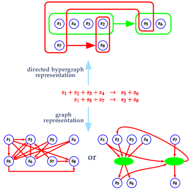
We modeled various metabolic and biochemical reactions as directed hypergraphs. Each reaction in the data had always at least one reactant but sometimes did not have a product. We represent a reaction of the form “”, where ’s are the reactants, ’s are the products, as a directed hyperedge (see Fig. 4) with and 111If the reaction times are known accurately then they can be used as the weights of the corresponding hyperedges.. In other words, each hyperedge points from the set of reactants to the set of products of the corresponding reaction. For reactions of the form “” without a product we use for a unique node named “” following the same conventions used in the network science literature (note that there is exactly one node in the entire hypergraph and it does not appear in for any hyperedge in the hypergraph). All the directed hypergraphs that we construct are weakly connected. We computed some first-order statistics of the constructed directed hypergraphs as shown in Table 2. We show in Fig. 4 a visual comparison of our hypergraph-theoretic representation with two common graph-theoretic representations of biochemical reactions.
III.2.2 Undirected Hypergraphs
The hypergraph has a node corresponding to every authors and an undirected hyperedge with corresponding to each paper co-authored by authors . For the Csp dataset, we build an undirected hypergraph out of the papers and take the largest connected component as our input undirected hypergraph. For the Nsp dataset, we found the largest connected component in the resulting undirected hypergraph of papers, and took that connected component as our input undirected hypergraph. We computed some first-order statistics of the constructed undirected hypergraphs as shown in Table 3. We show in Fig. 5 a visual comparison of our hypergraph-theoretic representation with a common graph-theoretic representation of co-authorship relationships.
|
|||||||
| degree | |||||||
| average | max | min | |||||
| Csp dataset | |||||||
| Nsp dataset | |||||||
III.3 Proof of Inapplicability of Normalized Ricci Flow equation (4) to graphs
The following theorem shows that there are infinitely many graphs for which the normalized Ricci flow equation (4) will make negative for some edge thus rendering the iterative process in (4) impossible to execute beyond the first step.
Theorem 1.
For all sufficiently large , there exists an undirected graph on nodes for which for some edge of .
Proof.
For convenience and ease of proof, we first explicitly state the standard definition of the Ricci curvature for an undirected graph where the weight is for every edge [37, 24, 25, 26, 27, 70, 95]. Consider an edge of our input (undirected unweighted) graph . For a node of , let and denote the closed neighborhood and the degree of in , respectively. Let and denote the two uniform distributions over the nodes in and , respectively. Extend the distributions and to all nodes in by assigning zero probabilities to nodes in and , respectively. The Ollivier-Ricci curvature of the edge is then defined as
| (14) |
where we use the same calculations of Emd as in Section II.1.
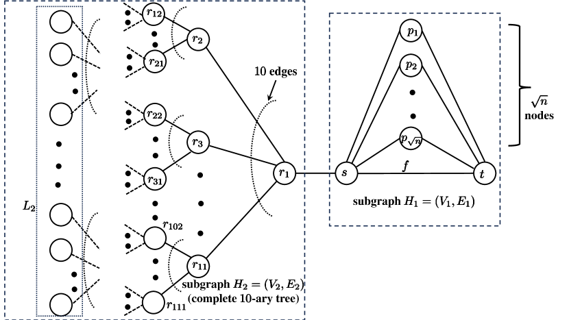
We will show the graph of edges where for every edge (and thus the sum of all edge weights is ). For this case, for and an edge of equation (4) simplifies to
It thus suffices to show the graph with an edge satisfying . We show this by showing a graph of nodes in which and for some positive constant . Our graph , as shown in Fig. 6, consists of two subgraphs and connected by an edge, where has nodes and edges is a complete -ary tree having nodes and edges. (since the graph is unweighted, we omit mentioning the weights of the edges). Thus, the total number of edges of is . Let be the set of leaf nodes of . We calculate the number of leaves of in the following simple manner. Letting be the depth of , we have . This gives the number of leaves of as . The edge shown in Fig. 6 is the edge for which we will show that .
Consider any edge of and the associated distributions and as defined before. The (standard) total variation distance between the two distributions and is defined as
By Proposition 1 of [70] we have
| (15) |
Now suppose that the following condition holds for the edge :
| (16) |
Using the discussions surrounding Proposition 1 and Proposition 2 of [70], we get the following bound for this case:
| (17) |
Finally, suppose that edge satisfies . Since for all , in this case we get the following bound:
| (18) |
We now use relatively straightforward calculations to calculate the Ricci curvature values of various edges of :
- (i)
- (ii)
- (iii)
-
Since trivially for any edge for , we get
- (iv)
-
For any edge connecting a leaf node to another non-leaf node in , since and , using (18) we get , and thus
- (v)
Adding up the relevant quantities, we get . Since and is a constant, it now follows that , thus there exists a constant such that for all sufficiently large . ∎
III.4 Rapid Initial Convergence of the Ricci Flow for Directed and Undirected Hypergraphs
As we shown in Table 4 below, the first iteration in which the edge-weights converge under Equation (5) is a small number for all of our (directed and undirected) hypergraphs.
| Hypergraph name | |
|---|---|
| Escherichia Coli | |
| Homo Sapiens | |
| Helicobacter Pylori | |
| Methanosarcina berkeri str. Fusaro | |
| Mycobacterium Tuberculosis | |
| Synechococcus elongatus | |
| Synechocystis | |
| Csp dataset | |
| Nsp dataset |
Table 4 show fast initial convergence of Ricci flows via small value of the parameter . However, as mentioned in Section III.1, it is preferable to execute more iterations to ensure that the diffusion process has actually converged in several successive iterations based on the value of and that the quality parameters are within acceptable bounds. Moreover, even if is within acceptable bounds, some individual edge weights may still change significantly in subsequent iterations since the value of (cf. Equation (6)) may not be acceptably low, and this may lead to changes in the cores. In our case, we indeed found that further iterations produced decreasing values of leading to more stable cores (see Table 5).
| values at end of | |||||
| Hypergraph name | |||||
| Escherichia Coli | |||||
| Homo Sapiens | |||||
| Helicobacter Pylori | |||||
| Methanosarcina berkeri str. Fusaro | |||||
| Mycobacterium Tuberculosis | |||||
| Synechococcus elongatus | |||||
| Synechocystis | |||||
| Csp dataset | |||||
| Nsp dataset | |||||
| ‡the smallest value of for which | |||||
III.5 Final Cores and Their Qualities Determined by Our Algorithm
| Hypergraph | core quality parameters | ||||||||||
|---|---|---|---|---|---|---|---|---|---|---|---|
| Escherichia Coli | |||||||||||
| Homo Sapiens | |||||||||||
| Helicobacter Pylori | |||||||||||
| Methanosarcina berkeri str. Fusaro | |||||||||||
| Mycobacterium Tuberculosis | |||||||||||
| Synechococcus elongatus | |||||||||||
| Synechocystis | |||||||||||
|
|||||||||||
| Hypergraph | core quality parameters | |||||||||||||||||||||||||
| Csp dataset | ||||||||||||||||||||||||||
| Nsp dataset | ||||||||||||||||||||||||||
|
||||||||||||||||||||||||||
|
||||||||||||||||||||||||||
We report in Table 6 and Table 7 the cores found by our algorithm with their quality parameters via Equations (8)–(12). As can be seen, taken together the parameters , , , for directed hypergraphs and the parameters , , for undirected hypergraphs indicate a good quality of modularity and centrality of the cores and satisfy all the validity criteria set forth in Sections II.3.1–II.3.5. For example, for Synechococcus elongatus hyperedges with only nodes from the core both in their head and tail contributed on average to the in-degrees of the nodes and similarly hyperedges with only nodes from the core both in their head and tail contributed on average to the out-degrees of the nodes. Furthermore, for Synechococcus elongatus about of ordered pairs of nodes not in the core that were connected by a path lose this path when the core is removed, and ordered node pairs that stay connected increase their distance by about on average.
An inspection of the values in Table 6 and Table 7 shows that removal of the cores disconnect fewer pairs of nodes in the core for undirected hypergraphs as compared to the directed hypergrahs (i.e., the values are smaller than the values), even though the stretch factors of shortest paths surviving after core removals are comparable (i.e., the , values are of similar magnitudes to the values of ). There are two possible reasons for this behavior. Firstly, the sizes of cores for undirected hypergraphs are smaller than the typical core sizes of directed hypergraphs, and intuitively one would expect removal of fewer nodes to disconnect less number of remaining paths. Secondly, the directionality constraints on paths for directed hypergraphs (i.e., edges may not be traversed in the wrong direction) allow fewer avenues to “bypass” the nodes in the core; indeed, majority of biochemical reactions in our dataset are not bidirectional reactions.
In the following two sections, we comment on interpreting the cores and their implications to future research works.
III.5.1 Interpretation and Usefulness of Cores for Directed Hypergraphs (Metabolic Systems)
A core of the directed hypergraph corresponds to a set of molecules (reactants and/or products) in the biochemical system under consideration. Our analysis indicates the following properties for this subset of molecules:
-
(I)
The high values of and in Table 6 suggest that each molecule (node) in the core is highly dependent on other molecules (nodes) in the core, e.g., for another molecule in the core either and are both reactants in the same biochemical reaction, which itself is part of the core or one of the them is a product produced in a core biochemical reaction in which the other one is a reactant.
-
(II)
The values of and signify the importance of the molecules in the core in the overall functioning of the biochemical system in the following manner.
-
(A)
Consider an ordered pair which contributes towards the value of by losing their path when the core is removed. This implies that the production of can be significantly reduced or perhaps completely disrupted by the removal of the core .
-
(B)
Consider an ordered pair such that is large enough to contribute significantly towards the value of . Then removal of the core may significantly delay the production of by increasing the number of reactions needed for its production.
-
(A)
Since removal of the core(s) significantly affects the overall functioning of the biochemical system, one can conclude that the core plays a dominant role in the system. Following a standard practice used in computational biology, researchers may focus on the molecules in the core and their associated biochemical reactions for further computational analysis if the original system was too computationally intensive to analyse because of its size.
Removing a core by biological experiments
Perturbation experiments (e.g., genetic knockouts) are well-established biological method for probing the importance of biochemical entities. The best way to eliminate a chemical reaction is to knock out the enzyme that catalyzes the reaction. We briefly comment here on optimally designing the biological experimental mechanism to remove a core , assuming that we have the data corresponding to the enzymes for each reaction (our datasets did not provide this information). Let be the set of all biochemical reactions in which one or more members of appear as either a reactant or a product (or both); thus, disabling the reactions in will effectively disconnect the core . Let be the set of enzymes catalyzing the reactions from . Then, a minimal set of enzyme knockouts that can be used to disable all the reactions in can be determined by solving an appropriate minimum hitting set problem [14] defined such that the universe is and corresponding to each enzyme we have a set . The reader is referred to standard literatures in computer algorithms such as [96] for methods to solve a minimum hitting set problem efficiently.
III.5.2 Interpretation and Usefulness of Cores for Undirected Hypergraphs (Co-author Relationships)
A core of the undirected hypergraph corresponds to a set of authors. Below we explain what the core signifies in terms of its properties:
-
(I)
The values of in Table 7 suggest that the authors in form a “close group” of collaborators in the sense that they wrote more papers with each other as compared to with authors outside the core.
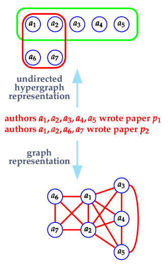
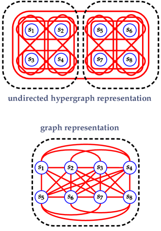
We show by an illustrative example that the above need not be the case if cores are found by graph-theoretic approaches. For some large even , suppose that authors wrote a paper, authors wrote a paper for and authors wrote a paper for (see Fig. 7 for a visual illustration when ). The standard graph-theoretic approach (cf. Fig. 5) will group all the nodes in the same core since they form a large -clique, whereas hypergraph-theoretic approach will correctly group them in two cores containing and , respectively.
-
(II)
The values of and signify the importance of the authors in in promoting collaborations between other researchers in the following manner. Note that for a path between nodes and and are co-authors for . Consider a pair of authors contributing towards the value of . This implies complete disruption of collaborations between any pairs of authors where one of them is in the set of authors reachable from via chains of collaboration and the other one is in the set of authors reachable from via chains of collaboration. If for a pair of authors was large enough to contribute significantly towards the value of then, even though some collaborative chains connecting and are not completely disrupted, they are elongated leading to a decrease in productivity.
IV Conclusion
In this article, we have designed and implemented an algorithmic paradigm for finding cores in edge-weighted directed and undirected hypergraphs using a hypergraph-curvature guided discrete time diffusion process, and have successfully applied our methods to seven metabolic hypergraphs and two social (co-authorship) hypergraphs. En route, we have also shown that an edge-weight re-normalization procedure in a prior research work for Ricci flows has undesirable properties. Finding cores of hypergraphs is still a relatively new research topic that is growing rapidly, and we expect that our our work will provide further impetus and guidance to this burgeoning research area. We conclude by listing a few research questions in this direction that may be of interest to researchers:
-
Our calculations of Ricci curvatures of directed hypergraphs in Section II.1.1 and directed hypergraphs in Section II.1.2 is a generalization of the corresponding calculations for undirected and directed graphs, respectively. However, it is possible to carry out these generalizations in different ways, and thus it will be of interest to know if other generalizations produce better qualities for cores of hypergraphs.
-
It would be of interest to see if the discrete time diffusion process using Ricci curvatures can be combined with random walks in hypergraphs [54] for application domains such as modular decompositions of graphs.
-
In spite of writing our code in Python (which runs slower than codes written in C or similar other programming languages) and using a single older (slower) laptop, we were able to finish our experimental work within reasonable time, and therefore we made no attempt to rewrite the code in a more suitable programming language, optimize the code and use a faster computational device. We believe this could be due to two reasons: (i) our hypergraphs were of moderate size (number of nodes) and moderate density (number and size of hyperedges), and (ii) our Ricci flow iterations converged within a few steps. However, computational speed could become an issue with larger hypergraphs or if Ricci flows required more steps to converge. Here we provide a few suggestions to researchers to overcome possible future computational bottlenecks. Note that the most computational intensive part of the curvature calculations involve the following two computational components: (a) computing the Earth Mover’s Distance (Emd) for each directed hyperedge or for each pair of nodes within an undirected hyperedge for every iteration, and (b) the all-pairs distance calculations once for the entire hypergraph for every iteration.
For all-pairs distance calculations we either used a straightforward adoption of Floyd-Warshall’s all-pair shortest path calculations with early terminations for graphs to our hypergraphs, or used a simple breadth-first-search based approach. However, the standard all-pairs-shortest-path problems for graphs have a long and rich algorithmic history [97] with strong connections to matrix multiplication algorithms [98, 99] and other problems [100], and future researchers could implement some of these advanced algorithmic methods for their computations. Note that in many applications it may even suffice to compute the distances approximately and in that case algorithms such as in [101] could be useful.
We have the following suggestions for future researchers regarding the Emd calculations:
-
Note that within each iteration, the calculations of the Emd values for the hyperedges can be done in parallel, and thus a clustered computing could be used.
-
*
Appendix A Details of Calculations of for Weighted Directed Hypergraphs in Section II.1.1
-
Initially, for all . In our subsequent steps, we will add to these values as appropriate.
-
We divide the total probability equally among the nodes in , thus “allocating” a value of to each node in question.
-
For every node with , we add to .
-
For every node with , we perform the following:
-
We divide the probability equally among the hyperedges such that , thus “allocating” a value of to each hyperedge in question.
-
For each such hyperedge such that , we divide the allocated value equally among the nodes in and add this values to the probabilities of these nodes. In other words, for every node we add to .
-
Note that the final probability for each node is calculated by summing all the contributions from each bullet point.
Acknowledgements.
We thank Katie Kruzan for useful discussions and help in debugging our software.References
- DasGupta and Liang [2016] B. DasGupta and J. Liang, Models and Algorithms for Biomolecules and Molecular Networks (Wiley-IEEE Press, New Jersey, 2016).
- Newman [2010] M. E. J. Newman, Networks: An Introduction (Oxford University Press, 2010).
- Albert and Barabási [2002] R. Albert and A.-L. Barabási, Statistical mechanics of complex networks, Reviews of Modern Physics 74, 47 (2002).
- Colizza et al. [2006] V. Colizza, A. Flammini, M. Serrano, and A. Vespignani, Detecting rich-club ordering in complex networks, Nature Physics 2, 110 (2006).
- Latora and Marchiori [2007] V. Latora and M. Marchiori, A measure of centrality based on network efficiency, New Journal of Physics 9, 188 (2007).
- Albert et al. [2011] R. Albert, B. DasGupta, R. Hegde, G. S. Sivanathan, A. Gitter, G. Gürsoy, P. Paul, and E. Sontag, Computationally efficient measure of topological redundancy of biological and social networks, Physical Review E 84, 036117 (2011).
- Bassett et al. [2011] D. S. Bassett, N. F. Wymbs, M. A. Porter, P. J. Mucha, J. M. Carlson, and S. T. Grafton, Dynamic reconfiguration of human brain networks during learning, Proceedings of the National Academy of Sciences 118, 7641 (2011).
- Battiston et al. [2020] F. Battiston, G. Cencetti, I. Iacopini, V. Latora, M. Lucas, A. Patania, J.-G. Young, and G. Petri, Networks beyond pairwise interactions: Structure and dynamics, Physics Reports 874, 1 (2020).
- Battiston et al. [2021] F. Battiston, E. Amico, A. Barrat, G. Bianconi, G. F. de Arruda, B. Franceschiello, I. Iacopini, S. Kéfi, V. Latora, Y. Moreno, M. M. Murray, T. P. Peixoto, F. Vaccarino, and G. Petr, The physics of higher-order interactions in complex systems, Nature Physics 17, 1093 (2021).
- Torres et al. [2021] L. Torres, A. S. Blevins, D. Bassett, and T. Eliassi-Rad, The why, how, and when of representations for complex systems, SIAM Review 63, 435 (2021), https://doi.org/10.1137/20M1355896 .
- Jeong et al. [2000] H. Jeong, B. Tombor, R. Albert, Z. N. Oltvai, and A.-L. Barabasi, The large-scale organization of metabolic networks, Nature 407, 651 (2000).
- DasGupta et al. [2007] B. DasGupta, G. A. Enciso, E. Sontag, and Y. Zhang, Algorithmic and complexity results for decompositions of biological networks into monotone subsystems, Biosystems 90, 161 (2007).
- Berge [1989] C. Berge, Hypergraphs: Combinatorics of Finite Sets, 2nd ed. (Elsevier Science Publishers, New York, NY, 1989).
- Garey and Johnson [1979] M. R. Garey and D. S. Johnson, Computers and Intractability: A Guide to the Theory of NP-Completeness, 1st ed. (W. H. Freeman, 1979).
- Bridson and Häfliger [1999] M. R. Bridson and A. Häfliger, Metric Spaces of Non-Positive Curvature, 1st ed. (Springer-Verlag Berlin Heidelberg, 1999).
- Berger [2003] M. Berger, A Panoramic View of Riemannian Geometry, 1st ed. (Springer-Verlag Berlin Heidelberg, 2003).
- Forman [2003] R. Forman, Bochner’s method for cell complexes and combinatorial ricci curvature, Discrete and Computational Geometry 29, 323 (2003).
- Sreejith et al. [2016] R. P. Sreejith, K. Mohanraj, J. Jost, E. Saucan, and A. Samal, Forman curvature for complex networks, Journal of Statistical Mechanics: Theory and Experiment 2016, 063206 (2016).
- Sreejith et al. [2017] R. P. Sreejith, J. Jost, E. Saucan, and A. Samal, Systematic evaluation of a new combinatorial curvature for complex networks, Chaos, Solitons and Fractals 101, 50 (2017).
- Weber et al. [2017] M. Weber, E. Saucan, and J. Jost, Characterizing complex networks with forman-ricci curvature and associated geometric flows, Journal of Complex Networks 5, 527 (2017).
- DasGupta et al. [2020] B. DasGupta, M. V. Janardhanan, and F. Yahyanejad, Why did the shape of your network change? (on detecting network anomalies via non-local curvatures), Algorithmica 82, 1741 (2020).
- Samal et al. [2018] A. Samal, R. P. Sreejith, J. Gu, S. Liu, E. Saucan, and J. Jost, Comparative analysis of two discretizations of ricci curvature for complex networks, Scientific Reports 8, 8650 (2018).
- Chatterjee et al. [2021] T. Chatterjee, R. Albert, S. Thapliyal, N. Azarhooshang, and B. DasGupta, Detecting network anomalies using forman-ricci curvature and a case study for human brain networks, Scientific Reports 11, 10.1038/s41598-021-87587-z (2021).
- Ollivier [2013] Y. Ollivier, A visual introduction to Riemannian curvatures and some discrete generalizations, in Analysis and Geometry of Metric Measure Spaces: Lecture Notes of the 50th Séminaire de Mathématiques Supérieures (SMS), Montréal, 2011, Vol. 56, edited by G. Dafni, R. J. McCann, and A. Stancu (American Mathematical Society, Providence, RI, USA, 2013) pp. 197–219.
- Ollivier [2009] Y. Ollivier, Ricci curvature of markov chains on metric spaces, Journal of Functional Analysis 256, 810 (2009).
- Ollivier [2010] Y. Ollivier, A survey of ricci curvature for metric spaces and markov chains, in Advanced Studies in Pure Mathematics, Vol. 57, edited by M. Kotani, M. Hino, and T. Kumagai (Mathematical Society of Japan, 2010) pp. 343–381.
- Ollivier [2007] Y. Ollivier, Ricci curvature of metric spaces, Comptes Rendus Mathematique 345, 643 (2007).
- Asoodeh et al. [2018] S. Asoodeh, T. Gao, and J. Evans, Curvature of hypergraphs via multi-marginal optimal transport, in 2018 IEEE Conference on Decision and Control (2018) pp. 1180–1185.
- Eidi and Jost [2020] M. Eidi and J. Jost, Ollivier ricci curvature of directed hypergraphs, Scientific Reports 10, 12466 (2020).
- Coupette et al. [2023] C. Coupette, S. Dalleiger, and B. Rieck, Ollivier-ricci curvature for hypergraphs: A unified framework, in The Eleventh International Conference on Learning Representations (2023).
- Akamatsu [2022] T. Akamatsu, A new transport distance and its associated ricci curvature of hypergraphs, Analysis and Geometry in Metric Spaces 10, 90 (2022).
- Leal et al. [2021] W. Leal, G. Restrepo, P. F. Stadler, and J. Jost, Forman-ricci curvature for hypergraphs, Advances in Complex Systems 24, 2150003 (2021), https://doi.org/10.1142/S021952592150003X .
- Hamilton [1982] R. S. Hamilton, Three-manifolds with positive Ricci curvature, Journal of Differential Geometry 17, 255 (1982).
- Perelman [2002] G. Perelman, The entropy formula for the ricci flow and its geometric applications, arXiv preprint arXiv:math/0211159v1 10.48550/arXiv.math/0211159 (2002).
- Ni et al. [2019] C.-C. Ni, Y.-Y. Lin, F. Luo, and J. Gao, Community detection on networks with ricci flow, Scientific Reports 9, 9984 (2019).
- Sia et al. [2019] J. Sia, E. Jonckheere, and P. Bogdan, Ollivier-ricci curvature-based method to community detection in complex networks, Scientific Reports 9, 9800 (2019).
- Lai et al. [2022] X. Lai, S. Bai, and Y. Lin, Normalized discrete ricci flow used in community detection, Physica A: Statistical Mechanics and its Applications 597, 127251 (2022).
- Weber et al. [2016] M. Weber, J. Jost, and E. Saucan, Forman-ricci flow for change detection in large dynamic data sets, Axioms 5, 10.3390/axioms5040026 (2016).
- Cohen et al. [2022] E. Cohen, Y. Nachshon, A. Maril, P. M. Naim, J. Jost, and E. Saucan, Object-based dynamics: Applying forman-ricci flow on a multigraph to assess the impact of an object on the network structure, Axioms 11, 10.3390/axioms11090486 (2022).
- Ni et al. [2018] C.-C. Ni, Y.-Y. Lin, J. Gao, and X. Gu, Network alignment by discrete ollivier-ricci flow, in Graph Drawing and Network Visualization, edited by T. Biedl and A. Kerren (Springer International Publishing, 2018) pp. 447–462.
- Kim et al. [2023] J. Kim, H. J. Jeong, S. Lim, and J. Kim, Effective and efficient core computation in signed networks, Information Sciences 634, 290 (2023).
- Fornito et al. [2016] A. Fornito, A. Zalesky, and E. Bullmore, Fundamentals of brain network analysis, 1st ed. (Academic press, 2016).
- Sporns and Betzel [2016] O. Sporns and R. F. Betzel, Modular brain networks, Annual Review of Psychology 67, 613 (2016).
- Harriger et al. [2012] L. Harriger, M. P. van den Heuvel, and O. Sporns, Rich club organization of macaque cerebral cortex and its role in network communication, PLoS ONE 7, e46497 (2012).
- Kitazono et al. [2020] J. Kitazono, R. Kanai, and M. Oizumi, Efficient search for informational cores in complex systems: Application to brain networks, Neural Networks 132, 232 (2020).
- Newman and Girvan [2004] M. E. J. Newman and M. Girvan, Finding and evaluating community structure in networks, Physical Review E 69, 026113 (2004).
- Leicht and Newman [2008] E. A. Leicht and M. E. J. Newman, Community structure in directed networks, Physical Review Letters 100, 118703 (2008).
- Newman [2006] M. E. J. Newman, Modularity and community structure in networks, Proceedings of the National Academy of Sciences 103, 8577 (2006), https://www.pnas.org/content/103/23/8577.full.pdf .
- DasGupta and Desai [2013] B. DasGupta and D. Desai, On the complexity of Newman’s community finding approach for biological and social networks, Journal of Computer and System Sciences 79, 50 (2013).
- DasGupta [2014] B. DasGupta, Computational complexities of optimization problems related to model based clustering of networks, in Optimization in Science and Engineering, edited by T. Rassias, C. Floudas, and S. Butenko (Springer, New York, NY, 2014) pp. 97–113.
- Tudisco and Higham [2023] F. Tudisco and D. J. Higham, Core-periphery detection in hypergraphs, SIAM Journal on Mathematics of Data Science 5, 1 (2023), https://doi.org/10.1137/22M1480926 .
- Chien et al. [2018] I. Chien, C.-Y. Lin, and I.-H. Wang, Community detection in hypergraphs: Optimal statistical limit and efficient algorithms, in Proceedings of the Twenty-First International Conference on Artificial Intelligence and Statistics, Proceedings of Machine Learning Research, Vol. 84, edited by A. Storkey and F. Perez-Cruz (PMLR, 2018) pp. 871–879.
- Ruggeri et al. [2023] N. Ruggeri, M. Contisciani, F. Battiston, and C. D. Bacco, Community detection in large hypergraphs, Science Advances 9, 10.1126/sciadv.adg9159 (2023), https://www.science.org/doi/pdf/10.1126/sciadv.adg9159 .
- Carletti et al. [2021] T. Carletti, D. Fanelli, and R. Lambiotte, Random walks and community detection in hypergraphs, Journal of Physics: Complexity 2, 015011 (2021).
- Eriksson et al. [2021] A. Eriksson, D. Edler, A. Rojas, M. de Domenico, and M. Rosvall, How choosing random-walk model and network representation matters for flow-based community detection in hypergraphs, Communications Physics 4, 1093 (2021).
- Kritschgau et al. [2024] J. Kritschgau, D. Kaiser, O. A. Rodriguez, I. Amburg, J. Bolkema, T. Grubb, F. Lan, S. Maleki, P. Chodrow, and B. Kay, Community detection in hypergraphs via mutual information maximization., Scientific Reports 14, 10.1038/s41598-024-55934-5 (2024).
- Zhen and Wang [2023] Y. Zhen and J. Wang, Community detection in general hypergraph via graph embedding, Journal of the American Statistical Association 118, 1620 (2023), https://doi.org/10.1080/01621459.2021.2002157 .
- Eriksson et al. [2022] A. Eriksson, T. Carletti, R. Lambiotte, A. Rojas, and M. Rosvall, Flow-based community detection in hypergraphs, in Higher-Order Systems, edited by F. Battiston and G. Petri (Springer International Publishing, Cham, 2022) pp. 141–161.
- Mancastroppa et al. [2023] M. Mancastroppa, I. Iacopini, G. Petri, and A. Barrat, Hyper-cores promote localization and efficient seeding in higher-order processes, Nature communications 14, 6223 (2023).
- Mancastroppa et al. [2024] M. Mancastroppa, I. Iacopini, G. Petri, and A. Barrat, The structural evolution of temporal hypergraphs through the lens of hyper-cores, EPJ Data Science 13, 10.1140/epjds/s13688-024-00490-1 (2024).
- Xu et al. [2023] Y. Xu, F. Zhang, and B. Liu, The decomposition and maintenance of hypercores on edge-weighted hypergraphs, Mathematical Foundations of Computing (2023).
- Pretolani [2013] D. Pretolani, Finding hypernetworks in directed hypergraphs, European Journal of Operational Research 230, 226 (2013).
- Volpentesta [2008] A. P. Volpentesta, Hypernetworks in a directed hypergraph, European Journal of Operational Research 188, 390 (2008).
- Albert et al. [2014] R. Albert, B. DasGupta, and N. Mobasheri, Topological implications of negative curvature for biological and social networks, Physical Review E 89, 032811 (2014).
- Burt [1992] R. S. Burt, Structural Holes: The Social Structure of Competition (Harvard University Press, Cambridge, MA, USA, 1992).
- Mallows [1972] C. L. Mallows, A Note on Asymptotic Joint Normality, The Annals of Mathematical Statistics 43, 508 (1972).
- Rubner et al. [1998] Y. Rubner, C. Tomasi, and L. J. Guibas, A metric for distributions with applications to image databases, in Sixth International Conference on Computer Vision (IEEE Cat. No.98CH36271) (1998) pp. 59–66.
- Rubner et al. [2000] Y. Rubner, C. Tomasi, and L. J. Guibas, The earth mover’s distance as a metric for image retrieval, International Journal of Computer Vision 40, 99 (2000).
- Villani [2003] C. Villani, Topics in optimal transportation, in Graduate Studies in Mathematics, Vol. 58 (American Mathematical Society, Providence, RI, USA, 2003) pp. 197–219.
- Azarhooshang et al. [2020] N. Azarhooshang, P. Sengupta, and B. DasGupta, A review of and some results for ollivier-ricci network curvature, Mathematics 8, 10.3390/math8091416 (2020).
- Girvan and Newman [2002] M. Girvan and M. E. J. Newman, Community structure in social and biological networks, Proceedings of the National Academy of Sciences 99, 7821 (2002), https://www.pnas.org/content/99/12/7821.full.pdf .
- Koujaku et al. [2016] S. Koujaku, I. Takigawa, M. Kudo, and H. Imai, Dense core model for cohesive subgraph discovery, Social Networks 44, 143 (2016).
- Bonchi et al. [2021] F. Bonchi, D. García-Soriano, A. Miyauchi, and C. E. Tsourakakis, Finding densest k-connected subgraphs, Discrete Applied Mathematics 305, 34 (2021).
- Boob et al. [2020] D. Boob, Y. Gao, R. Peng, S. Sawlani, C. Tsourakakis, D. Wang, and J. Wang, Flowless: Extracting densest subgraphs without flow computations, in Proceedings of The Web Conference 2020, WWW ’20 (Association for Computing Machinery, New York, NY, USA, 2020) pp. 573–583.
- [75] C. Chekuri, K. Quanrud, and M. R. Torres, Densest subgraph: Supermodularity, iterative peeling, and flow, in Proceedings of the 2022 Annual ACM-SIAM Symposium on Discrete Algorithms (SODA), pp. 1531–1555, https://epubs.siam.org/doi/pdf/10.1137/1.9781611977073.64 .
- Fang et al. [2022] Y. Fang, W. Luo, and C. Ma, Densest subgraph discovery on large graphs: applications, challenges, and techniques, Proc. VLDB Endow. 15, 3766 (2022).
- Liu et al. [2022] X. Liu, T. Ge, and Y. Wu, A stochastic approach to finding densest temporal subgraphs in dynamic graphs, IEEE Transactions on Knowledge and Data Engineering 34, 3082 (2022).
- Luo et al. [2023] W. Luo, Z. Tang, Y. Fang, C. Ma, and X. Zhou, Scalable algorithms for densest subgraph discovery, in 2023 IEEE 39th International Conference on Data Engineering (ICDE) (2023) pp. 287–300.
- Ma et al. [2022] C. Ma, R. Cheng, L. V. S. Lakshmanan, and X. Han, Finding locally densest subgraphs: a convex programming approach, Proc. VLDB Endow. 15, 2719 (2022).
- Ma et al. [2021] C. Ma, Y. Fang, R. Cheng, L. V. S. Lakshmanan, W. Zhang, and X. Lin, On directed densest subgraph discovery, ACM Transaction Database Systems 46, 10.1145/3483940 (2021).
- Feige et al. [2001] U. Feige, D. Peleg, and G. Kortsarz, The dense k-subgraph problem, Algorithmica 29, 410 (2001).
- Bhaskara et al. [2010] A. Bhaskara, M. Charikar, E. Chlamtac, U. Feige, and A. Vijayaraghavan, Detecting high log-densities: an approximation for densest k-subgraph, in Proceedings of the Forty-Second ACM Symposium on Theory of Computing, STOC ’10 (Association for Computing Machinery, New York, NY, USA, 2010) pp. 201–210.
- Bera et al. [2022] S. K. Bera, S. Bhattacharya, J. Choudhari, and P. Ghosh, A new dynamic algorithm for densest subhypergraphs, in Proceedings of the ACM Web Conference 2022, WWW ’22 (Association for Computing Machinery, New York, NY, USA, 2022) pp. 1093–1103.
- Newman [2003] M. E. J. Newman, The structure and function of complex networks, SIAM Review 45, 167 (2003).
- Newman [2004] M. E. J. Newman, Detecting community structure in networks, European Physics Journal B 38, 321 (2004).
- Kannan et al. [1999] R. Kannan, P. Tetali, and S. Vempala, Simple markov-chain algorithms for generating bipartite graphs and tournaments, Random Structures & Algorithms 14, 293 (1999).
- King et al. [2016] Z. A. King, J. Lu, A. Dräger, P. Miller, S. Federowicz, J. A. Lerman, A. Ebrahim, B. O. Palsson, and N. E. Lewis, Bigg models: A platform for integrating, standardizing and sharing genome-scale models, Nucleic acids research 44, D515 (2016).
- Molontay and Nagy [2021] R. Molontay and M. Nagy, Twenty years of network science: A bibliographic and co-authorship network analysis, in Big Data and Social Media Analytics: Trending Applications, edited by M. Çakırtaş and M. K. Ozdemir (Springer International Publishing, Cham, 2021) pp. 1–24.
- Goldwasser and Micali [1984] S. Goldwasser and S. Micali, Probabilistic encryption, Journal of Computer and System Sciences 28, 270 (1984).
- Karp [1972] R. M. Karp, Reducibility among combinatorial problems, in Complexity of Computer Computations: Proceedings of a symposium on the Complexity of Computer Computations, edited by R. E. Miller, J. W. Thatcher, and J. D. Bohlinger (Springer US, Boston, MA, 1972) pp. 85–103.
- Nisan and Wigderson [1994] N. Nisan and A. Wigderson, Hardness vs randomness, Journal of Computer and System Sciences 49, 149 (1994).
- Barabási and Albert [1999] A.-L. Barabási and R. Albert, Emergence of scaling in random networks, Science 286, 509 (1999).
- Watts and Strogatz [1998] D. Watts and S. Strogatz, Collective dynamics of ‘small-world’ networks, Nature 393, 440 (1998).
- Note [1] If the reaction times are known accurately then they can be used as the weights of the corresponding hyperedges.
- DasGupta et al. [2023] B. DasGupta, E. Grigorescu, and T. Mukherjee, On computing discretized ricci curvatures of graphs: Local algorithms and (localized) fine-grained reductions, Theoretical Computer Science 975, 114127 (2023).
- Vazirani [2010] V. V. Vazirani, Approximation Algorithms, 1st ed. (Springer, Berlin, Heidelberg, 2010).
- Cormen et al. [2009] T. H. Cormen, C. E. Leiserson, R. L. Rivest, and C. Stein, Introduction to Algorithms, 3rd ed. (MIT Press and McGraw-Hill, 2009).
- Seidel [1995] R. Seidel, On the all-pairs-shortest-path problem in unweighted undirected graphs, Journal of Computer and System Sciences 51, 400 (1995).
- Zwick [2002] U. Zwick, All pairs shortest paths using bridging sets and rectangular matrix multiplication, Journal of the ACM 49, 289 (2002).
- Williams and Williams [2018] V. V. Williams and R. R. Williams, Subcubic equivalences between path, matrix, and triangle problems, Journal of the ACM 65, 1 (2018).
- Dor et al. [2000] D. Dor, S. Halperin, and U. Zwick, All-pairs almost shortest paths, SIAM Journal on Computing 29, 1740 (2000).
- Quanrud [2018] K. Quanrud, Approximating Optimal Transport With Linear Programs, in 2nd Symposium on Simplicity in Algorithms (SOSA 2019), OpenAccess Series in Informatics (OASIcs), Vol. 69, edited by J. T. Fineman and M. Mitzenmacher (Schloss Dagstuhl–Leibniz-Zentrum fuer Informatik, Dagstuhl, Germany, 2018) pp. 6:1—6:9.
- Dvurechensky et al. [2018] P. Dvurechensky, A. Gasnikov, and A. Kroshnin, Computational optimal transport: Complexity by accelerated gradient descent is better than by sinkhorn’s algorithm, in Proceedings of the 35th International Conference on Machine Learning, Proceedings of Machine Learning Research, Vol. 80, edited by J. Dy and A. Kraus (PMLR, 2018) pp. 1367—1376.