Turbulent-like flows in quasi two-dimensional dense suspensions of motile colloids
Abstract
Dense bacterial suspensions exhibit turbulent-like flows at low Reynolds numbers, driven by the activity of the microswimmers. In this study, we develop a model system to examine these dynamics using motile colloids that mimic bacterial locomotion. The colloids are powered by the Quincke instability, which causes them to spontaneously roll in a random-walk pattern when exposed to a square-wave electric field. We experimentally investigate the flow dynamics in dense suspensions of these Quincke random walkers under quasi two-dimensional conditions, where the particle size is comparable to the gap between the electrodes. Our results reveal an energy spectrum scaling at high wavenumbers as , which holds across a broad range of activity levels – controlled by the field strength – and particle concentrations. We observe that velocity time correlations decay within a single period of the square-wave field, yet an anti-correlation appears between successive field applications, indicative of a dynamic structural memory of the ensemble.
Swimming bacteria self-organize into macroscopic patterns such as swarms and dynamic clusters Copeland:2009 ; zhang:2009 ; zhang:2010 ; chen:2012 ; chen:2015 ; Beer:2020 ; Aranson:2022 . At high concentrations, turbulent-like motion emerges characterized by erratic flows and transient vortices Dombrowski:2004 ; Sokolov:2007 ; wensink2012 ; Dunkel:2013 ; Gachelin_2014 ; Zhou:2014 ; peng2021 . Unlike the classical hydrodynamic turbulence, which is a high-Reynolds number, inertia-dominated phenomenon, bacterial turbulence occurs at very low Reynolds numbers, where inertia is negligible, and is driven by the active motion of the microswimmers alert2022 . The energy spectrum in classical turbulence in two dimensions typically follows a power-law dependence on the wavenumber, , whereas for bacterial turbulence different power laws have been reported wensink2012 ; Liu-Cheng:2021SM ; wei2024 .
Active turbulence has been observed in various living fluids such as sperm creppy:2015 , microtubule-kinesin bundles (active nematics) Dogic:2012 ; Opathalage:2019 ; Sagues:2019 , and cell tissues Blanch:2019 ; lin2021 . The phenomenon generated a lot of theoretical effort SR:2002 ; Saintillan07 ; Saintillan:2011 ; Saintillan:2013 ; wensink2012 ; Dunkel:2013 ; Dunkel:2013b ; bratanov2015 ; giomi2015 ; James:2018 ; Doostmohammadi:2018 ; Linkmann:2019 ; Skultety-Morozov:2020 ; Shaebani:2020review ; qi2022 ; w.zantop2022 ; Keta:2024 ; yang2024shaping , to decipher how “activity engenders turbulence” Fraden:2019comm . Recently, a universal scaling of has been predicted and validated for two-dimensional active nematics systems martinez-prat2021 , and similar scaling has been observed in studies of bacterial turbulence transitioning from two-dimensional to three-dimensional flow, where such scaling is absent in purely two-dimensional conditions wei2024 . However, experimental research in bacterial turbulence lags the theoretical advances due to the challenges to have well defined and controllable conditions e.g., particle density, speed (i.e., activity) and locomotion type, when working with living microswimmers. Synthetic externally driven colloids offer an alternative platform for studying active turbulence nishiguchi2015 ; kokot2017active ; mecke2023simultaneous .
A promising model system to emulate bacterial flows is based on the Quincke rollers bricard2013 ; Driscoll:2019 ; BOYMELGREEN:2022 ; Diwakar:2022 ; Bishop:2023 . Their motility is due to an electrohydrodynamic instability which gives rise to a constant electric torque on the particles quincke1896 causing them to roll, if the particles are initially resting on the electrode. Quincke rollers exhibit a wide range of intricate collective behaviors bricard2013 ; bricard2015 ; chardac2021emergence ; zhang2020reconfigurable ; zhang2022 ; jorge2024active . Temporal modulation of the rollers’ activity through application of a square-wave electric field modifies the rollers persistence length resulting in even richer collective dynamics karani2019 ; zhang2021persistence ; zhang2022natphys . By adjusting the durations of the pulses, , and their spacing, , the trajectory of an isolated Quincke roller becomes a random walk, and the particle locomotion can be tuned to emulate various bacterial motility patterns karani2019 . Populations of Quincke random walkers exhibit behaviors reminiscent of bacterial suspensions such as dynamic clustering in semi-dilute suspensions karani2019 .
Here, we employ dense suspensions of Quincke random walkers to gain insights into the turbulent-like flows of bacterial and active fluids. We consider suspensions confined between two parallel walls with spacing comparable to the colloid diameter, and experimentally measure spatial velocity correlations, structure functions, and kinetic energy spectra under varying concentrations of suspensions and activity, which is modulated by the applied field strength.
I Experiment
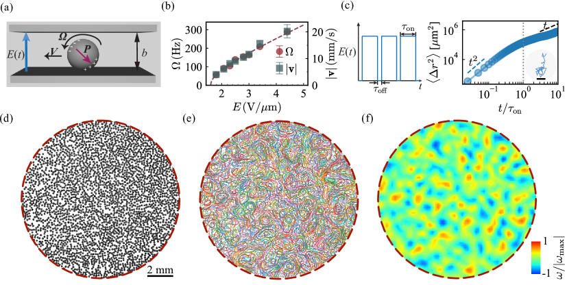
Spherical polymethyl methacrylate (PMMA) spheres (Phosphorex) with a diameter of are dispersed in a AOT-hexadecane solution (conductivity ). The experimental chamber consists of two cm2 ITO coated glass slides (Delta Technologies), separated by a ring-shaped Teflon tape with thickness of 120 , see Figure 1(a). The chamber is filled with the suspension solution. The particle motion and tracking is visualized using an inverted optical microscope (Zeiss) with 2X magnification mounted on a vibration isolation table (Kinetic Systems, Inc.). Videos were recorded at frame rates 500 or 1000 frames per second by a high speed camera (Photron SA 1.1). The system is powered by a pre-designed pulsed electric field supplied by a high voltage amplifier (Matsusada) controlled by a function generator (Agilent Technologies 33521A). Particle tracking, flow field reconstruction and data analysis are carried out by means of particle image velocimetry (PIV) or particle tracking velocimetry (PTV) using open source Python codes (OpenPIV alex2021 and Trackpy allan2024 ) as well as custom codes (see Appendix for details).
When a constant voltage is applied across the ITO electrodes, the particles become polarized due to the accumulation of free charges at their interfaces, generating an induced electric dipole oriented antiparallel to the applied electric field. Beyond a critical field strength, the dipole loses its symmetric orientation, triggering what is known as the Quincke electrorotation Lemaire:2002 ; Jones:1984 and a particle rolls along the surface with a constant speed bricard2013 ; pradillo2019 , see Figure 1(b). In our system, the typical threshold voltage for the onset of electrorotation is and roller velocities range from to .
When the electric field is pulsating, as shown in Figure 1(c), the behavior of the roller changes. The roller “runs” while the field is on and stops when the field is turned off. Once the field is turned on again, the roller chooses a new random direction of rolling karani2019 , which results in diffusive motion of the colloid. The colloid run-stop-turn random walk mimics the bacterial run-and-tumble motility. A dense suspension of Quincke random walkers exhibits turbulent-like flow, see Figure 1(d)-(f). In our experiments, we vary the field magnitude while maintaining fixed pulse durations and intervals . The off-time is much longer than the particle memory time, which is the Maxwell-Wagner polarization relaxation time , to ensure that the roller executes an uncorrelated random walk. sets the particle persistence length and it is chosen so that it is comparable to the collision time, which varies from to . The average collision time of the particles is estimated based on the average particle number density, , where is the number density of particles, is the particle’s diameter, is the average speed of the particles.
We use a ring-shaped Teflon tape as both a separator and a solid boundary to enclose the suspension solution. To prevent particles from becoming trapped between the glass slides and the tape during chamber assembly, the particles are concentrated to the central region of the chamber; the chamber is first filled with oil, and then a drop of concentrated suspension () is deposited in the middle of the chamber. The uniform particle region has a diameter of approximately 1.6 cm, which is twice the diameter of the recorded field of view. The total suspension region spans 2.2 cm in diameter. Due to the presence of a particle-free zone between the uniform particle region and the tape boundary, we observed a gradual decrease in suspension concentration within the field of view during the experiment. For the results reported later, the concentration value represents the average concentration in the field of view, with variations of less than over time.
II Results
II.1 Flow structure
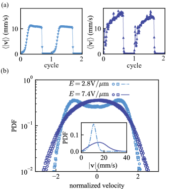
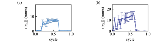
A unique feature of the Quincke random walkers is that when the field is on, they all run, and when the field is turned off, they all stop, see Fig. 2(a). At lower activity and particle fraction, , the flow driven by the colloids reaches a steady state within one cycle while the field is on. However, higher activity and particle numbers, , give rise to a more vigorous flow, which does not reach steady state within the period of the applied electric field. The collective dynamics mirrors the behavior of the isolated Quincke random walker, see Appendix, Figure 6. The difference in the flow development is due to the particle inertia pradillo2019 . Fig. 2(b) shows the velocity distribution for the experiments with low activity, low density () and higher activity, high density () systems. A bimodal structure of the PDF suggests that the particles are running with similar velocity; the sampling of the random velocity directions results in the two peaks kokot2019diffusive . At higher concentration, the PDF approaches a Gaussian distribution with a single peak due to the fact that particles experience multiple collisions in the same time period between two consecutive frames, , used to determine the velocity ().
To characterize the flow structure, we compute the velocity spatial correlation function, VCF,
| (1) |
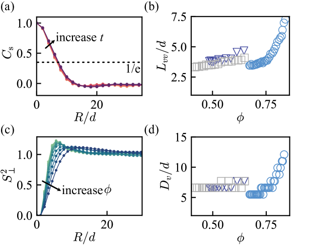
where is the field velocity, and is the spatial average over all positions . The velocity field is obtained directly from Particle Image Velocimetry (PIV) for experiments with dense suspensions or by interpolation based on individual particle velocity result from Particle Tracking Velocimetry (PTV) for experiments with low particle density . The VCF within the duration of one period of the applied field is plotted in Fig. 3(a). It shows velocity anticorrelation (negative VCF) typical for presence of vortices. If is sufficiently long, a single giant vortex—whose size is constrained by the system boundary— forms, as previously observed in experiments under weaker confinement zhang2022a ; bricard2013 . A single vortex would exhibit a velocity correlation value of . However, in our system, the presence of multiple vortices at different locations and of varying sizes results in a shallower minimum. Characteristic velocity correlation length, , defined from the decay of the velocity space correlation function, , increases with the particle fraction, see Fig. 3(b).
The velocity structure function provides further insight into the physics of active turbulence wensink2012 ; wei2024 . The normalized perpendicular structure function is defined as:
| (2) |
Here, is an orthogonal directions to . The maximum of corresponds to the effective vortex size . Fig.3(c) shows the as a function of at . The peak location, which corresponds to the mean vortex size , shifts to larger with the density. Likewise, the mean vortex size follows a similar trend as with the particle number density , see Fig. 3(d).
II.2 Kinetic energy spectrum
We next examine how the kinetic energy is distributed across different length scales for varying field strengths and particle concentrations. The energy spectrum, i.e., the energy of a vortex with size , is computed from the velocity field through the relation kraichnan1980 ; boffetta2012 ; martinez-prat2021 ; wensink2012 ; frisch1995
| (3) |
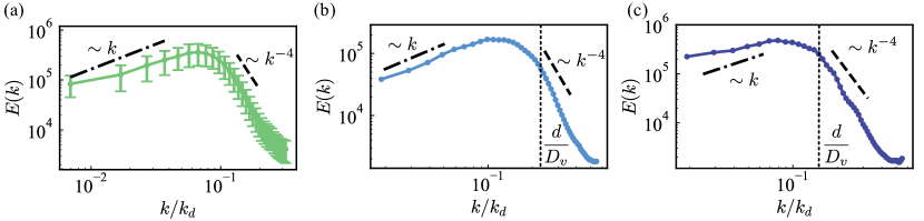
where is the wavenumber, is the system area and is the Fourier transformation of velocity. is the total energy per unit mass of the system. Fig. 4 shows the energy spectra for our system.
Different scaling laws have been predicted and observed for active nematics and bacterial systems, as reported in references giomi2015 ; martinez-prat2021 ; wei2024 . Despite the wide range of particle activities and concentrations in our experiments, the energy scaling law predominantly follows at large . This scaling holds in a regime of wavenumber smaller than the typical size of vortices, and when dissipation is dominated by the flow, rather than friction with the boundaries.
Our experiments also find exponential vortex size distribution (see Appendix Figure 7), which has been observed in active nematic turbulence and bacterial turbulence giomi2015 ; martinez-prat2021 ; wei2024 , where is found. This exponential distribution underlies the scaling for the energy density spectrum in such systems. The measurement of the vortex size from the previous section is indicated in the energy spectrum Fig.4(b-c), and roughly coincides with the wavenumber above which the scaling exists.
II.3 Temporal memory effects
In was recently demonstrated zhang2022natphys that Quincke rollers in a globally correlated collective state (vortex) spontaneously develop structural positional ordering that ”imprint” the chiral state of the system. Under a cessation and restoration of the activity facilitated by a pulsed field with both and significantly larger than all relevant timescales, a global vortex alternates its chiral state with each activity cycle. This periodic response, despite the absence of memory at the level of individual particles, was attributed to a phenomenon referred to as collective or ”structural memory”. To investigate whether a similar ”memory” phenomenon occurs in our system under a pulsating field with shorter , we compute the temporal correlations function of the velocity field
| (4) |
and the vorticity field,
| (5) |
Here, the system is divided into a square grid. is the average velocity at the cell ; is the total number of cells and denotes the time average. Similarly, we compute the vorticity field based on the velocity field and proceed to compute the vorticity temporal correlation function.
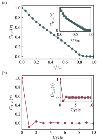
Within one cycle, see Figure 5(a), the time correlation function decays to zero, indicating that at a fixed location, the flow field decorrelates from its initial state, likely due to the particle collisions. Nevertheless, when the time correlation function is computed between the pulses (stroboscopically- at fixed time within each period), the correlation functions exhibit clear non-negligible anti-correlations after one cycle (see Figure 5(b)) indicative of the velocity and vorticity reversals in the ensemble during temporal activity cycling. This behavior is attributed to structural memory, facilitated by positional ordering of particles in self-organized vorticeszhang2022natphys . In our system under short activity pulses, local vortices do not coalesce into a giant vortex. Nonetheless, the formation of these locally correlated vortical states is the source of the anti-correlations in the system between the activity cycles. Only particles participating in local vortices contribute to the anti-correlations resulting in the correlation value significantly lower that (as it is with a global vortex state zhang2022natphys ). The signature of the collective ensemble memory is robust and easily detectable. Over time (beyond 2 cycles) the correlations between the activity cycles are suppressed as the locations of vortices get randomized.
III Conclusion
We have investigated active turbulence in a system of Quincke random walkers, a synthetic system which mimic the run-and-tumble behavior of bacteria. The Quincke random walkers provide a versatile experimental model of active matter to study the fundamental mechanisms of active turbulence. We demonstrated that the kinetic energy spectra follow scaling, consistent with the observations in very confined bacterial suspensions wei2024 . Our experiments indicate exponential vortex size distribution, which has been previously observed in active nematic turbulence and bacterial turbulence. In addition, we have found clear evidence of structural collective memory in this quasi-two-dimensional dense suspension. Our findings highlight the importance of transient dynamic memory in the ensemble, both at the particle level and collective, in accessing unconventional self-organized states.
IV Acknowledgment
The research of R.L. and P.V. was supported by NSF-DMR award 2004926. The research of A.S. was supported by the U.S. Department of Energy, Office of Science, Basic Energy Sciences, Materials Sciences and Engineering Division.
Appendix A Isolated Quincke Random Walker
The speed of an isolated Quincke random walker takes time to reach a steady state. At , the speed eventually stabilizes to a steady state. However, at , the particle’s speed exhibits oscillations with a larger amplitude when the field is applied, and it continues to increase throughout the runtime .
Appendix B Experimental Imaging and Analysis Methods
B.1 Imaging Setup and Parameters
For imaging, a high-speed camera (Photron SA 1.1) is employed in conjunction with a microscopy setup (Zeiss, 2x magnification). The frame rate (fps) is strategically selected to be either 500 or 1000, depending on the particle concentration and the applied field strength. This selection ensures that the motion of the particles is adequately resolved, facilitating accurate tracking and analysis of their dynamics under the experimental conditions.
B.2 Velocity and Vorticity Measurements
B.2.1 Dilute Suspensions: Particle Tracking Velocimetry (PTV)
In dilute suspensions (area fraction ), Particle Tracking Velocimetry (PTV) is employed to measure individual particle velocities. The Trackpyallan2024 library is utilized for this purpose. When dealing with images captured at different frame rates (fps) under varying field strengths or concentrations, the time interval used to link particles is carefully chosen such that the displacement of particles between frames remains within to of the particle diameter. This ensures accurate tracking without excessive ambiguity or loss of particles due to large displacements. The flow field is then reconstructed using cubic interpolation of the scattered particle data points to generate interpolated velocity values on a predefined grid. This interpolation is facilitated by the scipy.interpolate.griddata function with the cubic(2D) method.
B.2.2 Dense Suspensions: Particle Image Velocimetry (PIV)
For dense suspensions with an area fraction of particles , the suspension is treated as a continuum phase. In this regime, Particle Image Velocimetry (PIV) is utilized to determine the velocity field. The OpenPIValex2021 library in Python is employed to estimate the 2D velocity field on a 2D cubic grid. Averaging windows of size 20 pixels by 20 pixels are selected, corresponding approximately to 2 by 2 times the mean particle diameter of for Polymethyl methacrylate (PMMA) particles. This window size ensures statistical reliability while resolving spatial flow field structures on the order of a few bacterial lengths. A 50% overlap between neighboring bins is used to enhance spatial resolution and accuracy.
B.2.3 Vorticity Calculation
The vorticity of the flow is computed using a second-order central difference scheme, implemented through the numpy.gradient function, which calculates the spatial derivatives required for vorticity determination. The results were cross-validated using Richardson’s Extrapolation (four-point central), confirming consistency.
B.2.4 Vortex size distribution based on Okubo-Weiss (OW) parameter
The flows generated by our active system exhibit distinct vortex structures. In the main text, we employ the structure function to compute the average vortex size. Here, we further identify and characterize the size distribution of vortices using the Okubo-Weiss (OW) parameter giomi2015 ; martinez-prat2021 . The OW parameter is defined as
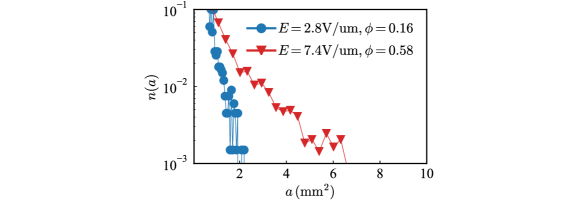
Regions where are identified as vortex regions. To analyze the vortex size distribution, we compute the histogram of the areas of connected vortex regions. This distribution, denoted as , represents the normalized frequency of vortices with area , where is the number of vortices of area . We find that follows an exponential distribution, , where is the mean vortex area and is the mean vortex diameter. In Figure 7 we show the distribution of vortex size for two typical experiments reported in the main text. Their fitted mean vortex diameters are and , which are comparable from the mean vortex diameter measured from structure function in the main text.
The exponential distribution of vortex areas is a key assumption in the theoretical framework used to explain the scaling of the energy spectrum in active systems, such as bacterial suspensions wei2024 and active nematics giomi2015 ; martinez-prat2021 .
B.3 Kinetic Energy Spectra
B.3.1 Energy Spectra Calculation
The total kinetic energy (per unit mass) of a 2D system is defined in real space as:
| (6) |
To analyze spectral energy distribution, we express the velocity field through its Fourier transform,
| (7) |
where the Fourier coefficients are given by,
| (8) |
Relating
| (9) | ||||
using the orthogonality of Fourier modes,
| (10) |
we simplify to,
| (11) |
To derive the radial energy spectrum , we convert to polar coordinates and average over angular dependence:
| (12) |
For homogeneous isotropic turbulence, the energy depends only on wavenumber magnitude . Defining the angle-averaged power spectrum,
| (13) |
we obtain the energy spectrum,
| (14) |
which satisfies and is the area.
B.3.2 Wiener-Khinchin Theorem
The energy spectrum can alternatively be computed from the velocity correlation function via the Wiener-Khinchin theoremfrisch1995 ,
| (15) |
Substituting into the expression for ,
| (16) |
where indicates averaging over the direction of (azimuthal angle ).
B.3.3 FFT and Windowing Effect
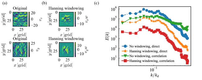
The derivation in B.3.2 used Wiener-Khinchin theorem to relate the energy spectrum with velocity spatial correlation function, which is valid in infinite domain. Our experiment is neither infinite nor periodic. The discontinuity of the boundary could effect the energy spectrum. We use a Hanning windowwilken2020 to process the velocity field measured from experiment, before computing energy spectrum directly ((14)) or from correlation function ((16)). The Hanning window is defines as . is the size of the square region of velocity field. We would like to point out the result difference from no windowing procedure and correlation equation ((16)), which shows the error of energy spectrum result without dealing with the in-continuous and non-periodic experimental data. In the main test, we use the direct method ((14)).
References
- [1] Matthew F. Copeland and Douglas B. Weibel. Bacterial swarming: a model system for studying dynamic self-assembly. Soft Matter, 5(6):1174–1187, 2009.
- [2] HP Zhang, Avraham Be’Er, Rachel S Smith, E-L Florin, and Harry L Swinney. Swarming dynamics in bacterial colonies. EPL (Europhysics Letters), 87(4):48011, 2009.
- [3] H. P. Zhang, Avraham Be’er, E.-L. Florin, and Harry L. Swinney. Collective motion and density fluctuations in bacterial colonies. Proceedings of the National Academy of Sciences of the United States of America, 107(31):13626–13630, August 2010.
- [4] Xiao Chen, Xu Dong, Avraham Be’er, Harry L Swinney, and HP Zhang. Scale-invariant correlations in dynamic bacterial clusters. Physical review letters, 108(14):148101, 2012.
- [5] Xiao Chen, Xiang Yang, Mingcheng Yang, and HP Zhang. Dynamic clustering in suspension of motile bacteria. EPL (Europhysics Letters), 111(5):54002, 2015.
- [6] Avraham Be’er, Bella Ilkanaiv, Renan Gross, Daniel B. Kearns, Sebastian Heidenreich, Markus Baer, and Gil Ariel. A phase diagram for bacterial swarming. COMMUNICATIONS PHYSICS, 3(1):66, APR 3 2020.
- [7] Igor S. Aranson. Bacterial active matter. REPORTS ON PROGRESS IN PHYSICS, 85(7):076601, JUL 1 2022.
- [8] C. Dombrowski, L. Cisneros, S. Chatkaew, R.E. Goldstein, and J.O. Kessler. Self-concentration and large-scale coherence in bacterial dynamics. Phys. Rev. Lett., 93:098103, Aug 2004.
- [9] Andrey Sokolov, Igor S. Aranson, John O. Kessler, and Raymond E. Goldstein. Concentration dependence of the collective dynamics of swimming bacteria. Phys. Rev. Lett., 98:158102, Apr 2007.
- [10] Henricus H. Wensink, Jörn Dunkel, Sebastian Heidenreich, Knut Drescher, Raymond E. Goldstein, Hartmut Löwen, and Julia M. Yeomans. Meso-scale turbulence in living fluids. Proceedings of the National Academy of Sciences, 109(36):14308–14313, September 2012.
- [11] Jörn Dunkel, Sebastian Heidenreich, Knut Drescher, Henricus H. Wensink, Markus Bär, and Raymond E. Goldstein. Fluid dynamics of bacterial turbulence. Phys. Rev. Lett., 110:228102, May 2013.
- [12] J Gachelin, A Rousselet, A Lindner, and E Clement. Collective motion in an active suspension ofEscherichia colibacteria. New Journal of Physics, 16(2):025003, feb 2014.
- [13] Shuang Zhou, Andrey Sokolov, Oleg D. Lavrentovich, and Igor S. Aranson. Living liquid crystals. PROCEEDINGS OF THE NATIONAL ACADEMY OF SCIENCES OF THE UNITED STATES OF AMERICA, 111(4):1265–1270, JAN 28 2014.
- [14] Yi Peng, Zhengyang Liu, and Xiang Cheng. Imaging the emergence of bacterial turbulence: Phase diagram and transition kinetics. Science Advances, 7(17):eabd1240, April 2021.
- [15] Ricard Alert, Jaume Casademunt, and Jean-François Joanny. Active turbulence. Annual Review of Fluid Mechanics, 2022.
- [16] Zhengyang Liu, Wei Zeng, Xiaolei Ma, and Xiang Cheng. Density fluctuations and energy spectra of 3d bacterial suspensions. SOFT MATTER, 17(48):10806–10817, DEC 15 2021.
- [17] Da Wei, Yaochen Yang, Xuefeng Wei, Ramin Golestanian, Ming Li, Fanlong Meng, and Yi Peng. Scaling Transition of Active Turbulence from Two to Three Dimensions. Advanced Science, n/a(n/a):2402643, 2024.
- [18] Hamid Karani, Gerardo E. Pradillo, and Petia M. Vlahovska. Tuning the random walk of active colloids: From individual run-and-tumble to dynamic clustering. Physical Review Letters, 123(20):208002, November 2019.
- [19] Adama Creppy, Olivier Praud, Xavier Druart, Philippa L Kohnke, and Franck Plourabou¥’e. Turbulence of swarming sperm. Physical Review E, 92(3):032722, 2015.
- [20] T. Sanchez, D.T. N. Chen, S.J. DeCamp, M. Heymann, and Z. Dogic. Spontaneous motion in hierarchically assembled active matter. Nature, 491(7424):431+, NOV 15 2012.
- [21] Achini Opathalage, Michael M. Norton, Michael P. N. Juniper, Blake Langeslay, S. Ali Aghvami, Seth Fraden, and Zvonimir Dogic. Self-organized dynamics and the transition to turbulence of confined active nematics. Proceedings of the National Academy of Sciences, 116(11):4788–4797, 2019.
- [22] Berta Martinez-Prat, Jordi Ignes-Mullol, Jaume Casademunt, and Francesc Sagues. Selection mechanism at the onset of active turbulence. NATURE PHYSICS, 15(4):362+, APR 2019.
- [23] C. Blanch-Mercader, V. Yashunsky, S. Garcia, G. Duclos, L. Giomi, and P. Silberzan. Turbulent dynamics of epithelial cell cultures. Phys. Rev. Lett., 120:208101, May 2018.
- [24] Shao-Zhen Lin, Wu-Yang Zhang, Dapeng Bi, Bo Li, and Xi-Qiao Feng. Energetics of mesoscale cell turbulence in two-dimensional monolayers. Communications Physics, 4(1):21, February 2021.
- [25] R. Aditi Simha and Sriram Ramaswamy. Hydrodynamic fluctuations and instabilities in ordered suspensions of self-propelled particles. Phys. Rev. Lett., 89:058101, Jul 2002.
- [26] D. Saintillan and M.J. Shelley. Orientational order and instabilities in suspensions of self-locomoting rods. Phys. Rev. Lett., 99(5), AUG 3 2007.
- [27] David Saintillan and Michael J. Shelley. Emergence of coherent structures and large-scale flows in motile suspensions. Journal of The Royal Society Interface, 9(68):571–585, 2012.
- [28] David Saintillan and Michael J. Shelley. Active suspensions and their nonlinear models. Comptes Rendus Physique, 14(6):497–517, 2013.
- [29] Jrn Dunkel, Sebastian Heidenreich, Markus Br, and Raymond E Goldstein. Minimal continuum theories of structure formation in dense active fluids. New Journal of Physics, 15(4):045016, apr 2013.
- [30] Vasil Bratanov, Frank Jenko, and Erwin Frey. New class of turbulence in active fluids. Proceedings of the National Academy of Sciences, 112(49):15048–15053, December 2015.
- [31] Luca Giomi. Geometry and topology of turbulence in active nematics. Physical Review X, 5(3):031003, July 2015.
- [32] Martin James, Wouter J. T. Bos, and Michael Wilczek. Turbulence and turbulent pattern formation in a minimal model for active fluids. Phys. Rev. Fluids, 3:061101, Jun 2018.
- [33] Amin Doostmohammadi, Jordi Ignes-Mullol, Julia M. Yeomans, and Francesc Sagues. Active nematics. NATURE COMMUNICATIONS, 9, AUG 21 2018.
- [34] Moritz Linkmann, Guido Boffetta, M. Cristina Marchetti, and Bruno Eckhardt. Phase transition to large scale coherent structures in two-dimensional active matter turbulence. Phys. Rev. Lett., 122:214503, May 2019.
- [35] Viktor Škultéty, Cesare Nardini, Joakim Stenhammar, Davide Marenduzzo, and Alexander Morozov. Swimming suppresses correlations in dilute suspensions of pusher microorganisms. Phys. Rev. X, 10:031059, Sep 2020.
- [36] M. Reza Shaebani, Adam Wysocki, Roland G. Winkler, Gerhard Gompper, and Heiko Rieger. Computational models for active matter. NATURE REVIEWS PHYSICS, 2(4):181–199, APR 2020.
- [37] Kai Qi, Elmar Westphal, Gerhard Gompper, and Roland G. Winkler. Emergence of active turbulence in microswimmer suspensions due to active hydrodynamic stress and volume exclusion. Communications Physics, 5(1):1–12, March 2022.
- [38] Arne W. Zantop and Holger Stark. Emergent collective dynamics of pusher and puller squirmer rods: Swarming, clustering, and turbulence. Soft Matter, 18(33):6179–6191, 2022.
- [39] Yann-Edwin Keta, Juliane U. Klamser, Robert L. Jack, and Ludovic Berthier. Emerging mesoscale flows and chaotic advection in dense active matter. Phys. Rev. Lett., 132:218301, May 2024.
- [40] Qianhong Yang, Maoqiang Jiang, Francesco Picano, and Lailai Zhu. Shaping active matter from crystalline solids to active turbulence. Nature Communications, 15(1):2874, 2024.
- [41] Seth Fraden. Turbulent beginnings. NATURE PHYSICS, 15(4):311–312, APR 2019.
- [42] Berta Martínez-Prat, Ricard Alert, Fanlong Meng, Jordi Ignés-Mullol, Jean-François Joanny, Jaume Casademunt, Ramin Golestanian, and Francesc Sagués. Scaling regimes of active turbulence with external dissipation. Physical Review X, 11(3):031065, September 2021.
- [43] Daiki Nishiguchi and Masaki Sano. Mesoscopic turbulence and local order in janus particles self-propelling under an ac electric field. Physical Review E, 92(5):052309, November 2015.
- [44] Gašper Kokot, Shibananda Das, Roland G Winkler, Gerhard Gompper, Igor S Aranson, and Alexey Snezhko. Active turbulence in a gas of self-assembled spinners. Proceedings of the National Academy of Sciences, 114(49):12870–12875, 2017.
- [45] Joscha Mecke, Yongxiang Gao, Carlos A Ramírez Medina, Dirk GAL Aarts, Gerhard Gompper, and Marisol Ripoll. Simultaneous emergence of active turbulence and odd viscosity in a colloidal chiral active system. Communications Physics, 6(1):324, 2023.
- [46] Antoine Bricard, Jean-Baptiste Caussin, Nicolas Desreumaux, Olivier Dauchot, and Denis Bartolo. Emergence of macroscopic directed motion in populations of motile colloids. Nature, 503(7474):95–98, November 2013.
- [47] Michelle Driscoll and Blaise Delmotte. Leveraging collective effects in externally driven colloidal suspensions: Experiments and simulations. Current opinion in colloid & interface science, 40:42–57, 2019.
- [48] Alicia Boymelgreen, Jarrod Schiffbauer, Boris Khusid, and Gilad Yossifon. Synthetic electrically driven colloids: a platform for understanding collective behavior in soft matter. Current Opinion in Colloid & Interface Science, page 101603, 2022.
- [49] Nidhi M Diwakar, Golak Kunti, Touvia Miloh, Gilad Yossifon, and Orlin D Velev. Ac electrohydrodynamic propulsion and rotation of active particles of engineered shape and asymmetry. Current Opinion in Colloid & Interface Science, page 101586, 2022.
- [50] Kyle J.M. Bishop, Sibani Lisa Biswal, and Bhuvnesh Bharti. Active colloids as models, materials, and machines. Annual Review of Chemical and Biomolecular Engineering, 14(Volume 14, 2023):1–30, 2023.
- [51] G. Quincke. Ueber rotationen im constanten electrischen felde. Annalen der Physik, 295:417 – 486, 03 1896.
- [52] Antoine Bricard, Jean-Baptiste Caussin, Debasish Das, Charles Savoie, Vijayakumar Chikkadi, Kyohei Shitara, Oleksandr Chepizhko, Fernando Peruani, David Saintillan, and Denis Bartolo. Emergent vortices in populations of colloidal rollers. Nature Communications, 6(1):7470, June 2015.
- [53] Amélie Chardac, Suraj Shankar, M Cristina Marchetti, and Denis Bartolo. Emergence of dynamic vortex glasses in disordered polar active fluids. Proceedings of the National Academy of Sciences, 118(10):e2018218118, 2021.
- [54] Bo Zhang, Andrey Sokolov, and Alexey Snezhko. Reconfigurable emergent patterns in active chiral fluids. Nature communications, 11(1):4401, 2020.
- [55] Bo Zhang, Alexey Snezhko, and Andrey Sokolov. Guiding self-assembly of active colloids by temporal modulation of activity. Physical Review Letters, 128(1):018004, January 2022.
- [56] Camille Jorge, Amélie Chardac, Alexis Poncet, and Denis Bartolo. Active hydraulics laws from frustration principles. Nature Physics, 20(2):303–309, 2024.
- [57] Bo Zhang, Hamid Karani, Petia M. Vlahovska, and Alexey Snezhko. Persistence length regulates emergent dynamics in active roller ensembles. Soft Matter, 17(18):4818–4825, 2021.
- [58] Bo Zhang, Hang Yuan, Andrey Sokolov, Monica Olvera De La Cruz, and Alexey Snezhko. Polar state reversal in active fluids. Nature Physics, 18(2):154–159, February 2022.
- [59] Alex Liberzon, Theo Käufer, Andreas Bauer, Peter Vennemann, and Erich Zimmer. OpenPIV/openpiv-python: OpenPIV-python v0.23.4. Zenodo, January 2021.
- [60] Daniel B. Allan, Thomas Caswell, Nathan C. Keim, Casper M. van der Wel, and Ruben W. Verweij. Soft-matter/trackpy: V0.6.4. Zenodo, July 2024.
- [61] E. Lemaire and L. Lobry. Chaotic behavior in electro-rotation. Physica A, 314(1-4):663–671, November 2002.
- [62] T. B. Jones. Quincke rotation of spheres. IEEE Trans. Industry Appl., 20:845–849, 1984.
- [63] Gerardo E. Pradillo, Hamid Karani, and Petia M. Vlahovska. Quincke rotor dynamics in confinement: Rolling and hovering. Soft Matter, 15(32):6564–6570, 2019.
- [64] Gašper Kokot, Andrej Vilfan, Andreas Glatz, and Alexey Snezhko. Diffusive ferromagnetic roller gas. Soft matter, 15(17):3612–3619, 2019.
- [65] Bo Zhang, Hang Yuan, Andrey Sokolov, Monica Olvera De La Cruz, and Alexey Snezhko. Polar state reversal in active fluids. Nature Physics, 18(2):154–159, February 2022.
- [66] R. H. Kraichnan and D. Montgomery. Two-dimensional turbulence. Reports on Progress in Physics, 43(5):547, May 1980.
- [67] Guido Boffetta and Robert E Ecke. Two-Dimensional Turbulence. Annual Review of Fluid Mechanics, 2012.
- [68] Uriel Frisch. Turbulence: The Legacy of A. N. Kolmogorov. Cambridge University Press, 1995.
- [69] Sam Wilken, Rodrigo E. Guerra, David J. Pine, and Paul M. Chaikin. Hyperuniform Structures Formed by Shearing Colloidal Suspensions. Physical Review Letters, 125(14):148001, September 2020.