Asymptotic Analysis and Practical Evaluation of Jump Rate Estimators in Piecewise-Deterministic Markov Processes

 
Abstract
Piecewise-deterministic Markov processes (PDMPs) offer a powerful stochastic modeling framework that combines deterministic trajectories with random perturbations at random times. Estimating their local characteristics (particularly the jump rate) is an important yet challenging task. In recent years, non-parametric methods for jump rate inference have been developed, but these approaches often rely on distinct theoretical frameworks, complicating direct comparisons. In this paper, we propose a unified framework to standardize and consolidate state-of-the-art approaches. We establish new results on consistency and asymptotic normality within this framework, enabling rigorous theoretical comparisons of convergence rates and asymptotic variances. Notably, we demonstrate that no single method uniformly outperforms the others, even within the same model. These theoretical insights are validated through numerical simulations using a representative PDMP application: the TCP model. Furthermore, we extend the comparison to real-world data, focusing on cell growth and division dynamics in Escherichia coli. This work enhances the theoretical understanding of PDMP inference while offering practical insights into the relative strengths and limitations of existing methods.

Keywords
Piecewise-deterministic Markov process; Growth-fragmentation model; Jump rate; Non-parametric estimation; Consistency; Central limit theorem; Vector-valued martingale

Author affiliations
Romain Azaïs, Inria team MOSAIC, Lyon, France
Solune Denis, Univ Angers, CNRS, LAREMA, SFR MATHSTIC, F-49000 Angers, France

Acknowledgment
This work has been supported by the Inria Action Exploratoire ALAMO. Solune Denis also thanks the Chair Stress Test, RISK Management and Financial Steering of the Foundation École Polytechnique, and the France 2030 program Centre Henri Lebesgue ANR-11-LABX-0020-01.
 

1 Introduction

1.1 Problem formulation

Piecewise-deterministic Markov processes (commonly abbreviated as PDMPs) were introduced by Davis in [10, 11] as a broad category of continuous-time stochastic models that exclude diffusion. These processes are well-suited for modeling deterministic dynamics where randomness manifests through discrete events. The motion of a PDMP on $\mathbb{R}^{d}$ (endowed with the Borel algebra $\mathcal{B}(\mathbb{R}^{d})$) is defined from its local characteristics:

• $\Phi:\mathbb{R}\times\mathbb{R}^{d}\to\mathbb{R}^{d}$ is the deterministic flow, which satisfies the semi-group property,

  $$\forall\,x\in\mathbb{R}^{d},~\forall\,t,\,s\in\mathbb{R},~\Phi(t+s|x)=\Phi(s|\Phi(t|x)).$$

  In some contexts, $\Phi(\cdot|x)$ will also be denoted $\Phi_{x}$.

• $\lambda:\mathbb{R}^{d}\to\mathbb{R}_{+}$ is the jump rate, related to the flow by the following condition,

  $$\forall\,x\in E,~\exists\,\varepsilon>0,~\int_{0}^{\varepsilon}\lambda(\Phi(t|x))\mathrm{d}t<\infty.$$

• $Q:\mathcal{B}(\mathbb{R}^{d})\times\mathbb{R}^{d}\to[0,1]$ is the transition kernel such that,

  $$\forall\,x\in\mathbb{R}^{d},~Q(\mathbb{R}^{d}\setminus\{x\}|x)=1.$$

The jump mechanism, that is, the discrete part of the dynamics, can be expressed as follows. Starting from $X_{0}$ at $T_{0}=0$, for any integer $n$,

$$\mathbb{P}(T_{n+1}-T_{n}>t\,|\,X_{T_{n}},T_{n}) = \exp\left(-\int_{0}^{t}\lambda\left(\Phi(s|X_{T_{n}})\right)\mathrm{d}s\right),$$

$$\mathbb{E}\left[\varphi(X_{T_{n+1}})\,|\,\Phi(T_{n+1}-T_{n}|X_{T_{n}})\right] = \int_{\mathbb{R}^{d}}\varphi(z)\,Q\left(\mathrm{d}z|\Phi(T_{n+1}-T_{n}|X_{T_{n}})\right).$$

These equations iteratively define the jump times $T_{n}$ and the post-jump locations $Z_{n}=X_{T_{n}}$. Between two consecutive jump times $T_{n}$ and $T_{n+1}$, the motion is expressed as,

$$\forall\,T_{n}\leq t<T_{n+1},~X_{t}=\Phi(t-T_{n}|X_{T_{n}}).$$

Beyond jump times and post-jump locations, one may also consider the inter-jumping times $S_{n}=T_{n}-T_{n-1}$ and the pre-jump locations $Z_{n}^{-}=\Phi(S_{n}|Z_{n-1})$.

If the process evolves in continuous time, all randomness is contained in the discrete-time characteristics $Z_{n}$, $Z_{n}^{-}$, $S_{n}$, and $T_{n}$. For example, when the flow is known, it is sufficient to know the pair $(Z_{n},S_{n+1})$ (or $(Z_{n},Z_{n+1}^{-})$), which notably form Markov chains, to reconstruct the entire trajectory.

Given the wide range of applications for this class of stochastic processes (in reliability, biology, insurance, see for instance [8, 12, 17] and references therein), the question of estimating local characteristics is crucial. Several statistical frameworks can be considered for this purpose. In this paper, we adopt a particularly general framework, aiming not only to develop statistical methods that can be applied to a large variety of problems, but also to better understand what distinguishes PDMPs. Specifically, we focus on the non-parametric estimation of the jump rate $\lambda$. To this end, we assume that the first $n$ jumps of a single trajectory are observed. Moreover, the flow is known, which implies that the discrete-time observation scheme is equivalent to assuming continuous-time observation of the entire trajectory. We consider general processes without imposing specific assumptions on the flow, the transition kernel, or the jump rate. However, to ensure convergence properties of the estimators (as $n$ tends to infinity), it is typically necessary to impose an ergodicity assumption, which can be applied either to the embedded chain $(Z_{n},S_{n+1})$ or to the continuous-time process $X_{t}$ [9].

1.2 Estimation strategies: a commented state-of-the-art

We review here, in chronological order, the non-parametric methods developed in the literature to estimate the jump rate of a general PDMP observed in long time. We also highlight (in Remarks 1.1, 1.2 and 1.3) some connections and similarities in the construction of estimators that were not reported in the bibliography.

Here and throughout the paper, $K^{d}$ denotes a kernel function in dimension $d$, i.e. a density on $\mathbb{R}^{d}$. To shorten equations, $K_{h}^{d}=K^{d}(\cdot/h)/h^{d}$ for any $h>0$. In addition, we omit the exponent when $d=1$, i.e. $K^{1}=K$. Importantly, the PDMP of interest $X_{t}$ is supposed to admit a unique invariant measure $\mu^{\text{\tiny CT}}$. Additionally, $\mu$ represents the invariant distribution of post-jump locations $Z_{n}$, while $\mu^{-}$ denotes the invariant distribution of pre-jump locations $Z_{n}^{-}$.

Fujii (2013)

The method designed in [16] to estimate the jump rate of a PDMP is based on Rice’s formula derived for one-dimensional processes in [6], which highlights the link between local time and stationary distribution. The author assumes that the flow of the PDMP under consideration $X_{t}$ is of the form,

$$\Phi(t|x)=x+\int_{0}^{t}\Delta(\Phi(s|x))\mathrm{d}s,$$ (1)

where $\Delta$ is a real-valued function such that $\inf\Delta>0$, and defines the local time of $X_{t}$ as

$$r(x)=\frac{\#\{t\in[0,T]\,:\,X_{t}=x\}}{\Delta(x)}.$$

After noting that the normalized local time $r(x)/T$ estimates the invariant density (of the continuous-time process) $\mu^{\text{\tiny CT}}(x)$, the author turns to the estimation of the jump rate and proposes to estimate $\lambda(x)$ by $\widehat{\lambda}_{T}(x)=TA(x)/r(x)$, with

$$A(x)=\frac{1}{T}\int_{0}^{T}\int_{\mathbb{R}_{+}}K_{h_{T}}\left(X_{t^{-}}-x\right)\mathrm{d}\chi(t,z),$$

where $\chi$ is the counting measure defined by

$$\chi(t,A)=\#\{n\in\mathbb{N}\,:\,T_{n}\leq t,\,Z_{n}\in A\}.$$

Under the assumption that jumps are only additive and downwards, the uniform convergence (when $T$ goes to infinity) in probability of this estimate is notably established. It should be noted that the observation scheme deviates from the one presented earlier in this paper: the observation window is in the time of the process $X_{t}$ and not in the discrete time of the embedded chain.

Remark 1.1.

Denoting $n_{T}$ the (random) number of jumps before $T$ and using the monotonicity of the flow, we rewrite Fujii’s estimator in the more conventional form,

$$\widehat{\lambda}_{T}(x)=\Delta(x)\times\frac{\frac{1}{n_{T}}\sum_{i=1}^{n_{T}}K_{h_{T}}(Z_{i}^{-}-x)}{\frac{1}{n_{T}}\sum_{i=0}^{n_{T}-1}\mathbbm{1}_{\{Z_{i}\leq x<Z_{i+1}^{-}\}}}.$$ (2)

Interestingly, the numerator is a kernel estimator of the invariant distribution $\mu^{-}$ while the denominator is the empirical version of $\mathbb{P}_{\mu}(Z_{0}\leq x<Z_{1}^{-})$.

Azaïs, Dufour and Gégout-Petit (2014)

The approach developed in [4] relies on the multiplicative intensity model developed by Aalen [1] (see also [2]). To estimate a jump rate $\lambda$, this method consists in exhibiting a counting process $N(t)$ whose stochastic intensity is of the form $\lambda(t)Y(t)$ for some predictable process $Y(t)$, i.e. such that the process $M(t)=N(t)-\int_{0}^{t}\lambda(s)Y(s)\mathrm{d}s$ is a continuous-time martingale. In PDMPs, conditionally on $Z_{i}$, the intensity of the one-jump process $\mathbbm{1}_{\{S_{i+1}\leq t\}}$ takes the expected form $\lambda(\Phi(t|Z_{i}))\mathbbm{1}_{\{S_{i+1}\geq t\}}$. Unfortunately, the sum over $i$ of these elementary martingales is generally not a martingale, which prevents the authors from applying the multiplicative intensity model directly.

In order to overcome this obstacle, the authors look at the law of the one-jump process conditionally on $Z_{i}$ but also on the future post-jump location $Z_{i+1}$, and obtain an explicit formula for its intensity: this can be put into multiplicative form, and its deterministic component (the modified jump rate) depends on time and two spatial variables (previous and future post-jump locations). In this case, the sum over $i$ remains a martingale, enabling the application of the multiplicative intensity model and thus the estimation of the modified jump rate.

The return to the jump rate of interest is also studied, leading to an estimate of the conditional density of inter-jumping times. The main drawback of this technique is that, in order to return to the quantity of interest, it requires integration over the whole space (with respect to the second spatial variable, i.e. the future post-jump location), even for local estimation. Nevertheless, convergence in probability, uniform on any compact set, of the conditional density estimator is demonstrated for processes on very general spaces (more general than $\mathbb{R}^{d}$) and involving forced jumps at the boundary.

Azaïs and Muller-Gueudin (2016)

The key of [5] is the fact that the jump rate of interest can be written as

$$\lambda(\Phi(t|x))=\frac{\mu(x)f(t|x)}{\mu(x)G(t|x)},$$

where the numerator is the invariant density of $(Z_{n},S_{n+1})$ at $(x,t)$ and the denominator is the measure of $(Z_{n},\mathbbm{1}_{\{S_{n+1}>t\}})$ at $(x,1)$ under the invariant distribution. Both are estimated using recursive kernel methods. Under mainly an ergodicity condition, pointwise almost sure convergence and asymptotic normality with expected rate $\sqrt{n(h_{n}^{\textrm{\tiny s}})^{d}h_{n}^{\textrm{\tiny t}}}$ of this estimator have been established in [5] for general PDMPs (with forced jumps) on $\mathbb{R}^{d}$. In this context, the authors notice that any couple $(\xi,\tau_{x}(\xi))$ such that $\Phi(\tau_{x}(\xi)|\xi)=x$ provides a consistent estimator of $\lambda(x)$. Indeed,

$$\widehat{\lambda\circ\Phi}_{n}(\tau_{x}(\xi)|\xi)\overset{\textrm{a.s.}}{\longrightarrow}\lambda(\Phi(\tau_{x}(\xi)|\xi))=\lambda(x).$$

It is then proposed to select the one with minimal asymptotic variance, which yields to maximize $\mu(\cdot)G(\tau_{x}(\cdot)|\cdot)$ on $\mathcal{C}_{x}=\{\xi\in\mathbb{R}^{d}\,:\,\exists\,t\geq 0,\,x=\Phi(t|\xi)\}$. Of course, this quantity is unknown but well-estimated by the denominator of $\widehat{\lambda\circ\Phi}_{n}(\tau_{x}(\xi)|\xi)$. The estimator obtained with optimal argument selection from the estimated criterion is not theoretically investigated but numerical simulations show its good properties.

Krell (2016)

PDMPs under consideration in [18] are one-dimensional and with a specific transition kernel of the form $Q(\cdot|x)=\delta_{\{h(x)\}}$. The statistical approach relies on the assumption that both the flow $\Phi(\cdot|x)$ (which will also be denoted $\Phi_{x}$ to shorten some equations) and the fragmentation function $h$ define a change of variable on $\mathbb{R}_{+}$, which makes this strategy specific to dimension $1$. In that context, it is shown that the targeted jump rate can be written as $\lambda(x)=\mu(h(x))/D^{\text{\tiny K}}(x)$, with

$$D^{\text{\tiny K}}(x)=\mathbb{E}_{\mu}\left[g_{Z_{0}}(h(x))\mathbbm{1}_{\{h(Z_{0})\leq h(x)\}}\mathbbm{1}_{\{Z_{1}\geq h(x)\}}\right],$$ (3)

where

$$g_{x}(y)=\displaystyle\frac{1}{(h\circ\Phi_{x})^{\prime}((h\circ\Phi_{x})^{-1}(y))}.$$

The numerator is evaluated as a kernel estimator of the invariant distribution $\mu$ composed with $h$, while the denominator is estimated by its empirical version. The main result of [18] states the convergence in $\mathbb{L}^{1}$-norm to $0$ of the square error with a rate depending on the regularity of $\lambda$. It should be noted that this estimator requires the knowledge of the transition kernel through the fragmentation function $h$. However, this part does not involve any randomness, which makes it easy to be estimated.

Remark 1.2.

In fact, $g_{x}(y)$ does not depend on x. Indeed, using the flow property, a direct calculus shows that

$$g_{x}(y)=\frac{(h^{-1})^{\prime}(y)}{\Delta(h^{-1}(y))},$$

where $\Delta(x)=\Phi_{x}^{\prime}(0)$ defines the flow (1) in Fujii’s method above. This allows us to simplify the formula (3) of $D^{\text{\tiny K}}(x)$,

$$D^{\text{\tiny K}}(x) = \frac{\mathbb{P}_{\mu}\left(Z_{0}\leq x,Z_{1}\geq h(x)\right)}{h^{\prime}(x)\Delta(x)},$$

$$= \frac{\mathbb{P}_{\mu}\left(Z_{0}\leq x<Z_{1}^{-}\right)}{h^{\prime}(x)\Delta(x)}.$$

Together with $\mu^{-}(x)=\mu(h(x))h^{\prime}(x)$, this yields

$$\lambda(x)=\frac{\Delta(x)\mu^{-}(x)}{\mathbb{P}_{\mu}\left(Z_{0}\leq x<Z_{1}^{-}\right)}.$$ (4)

This makes it possible to point out a remarkable connection with Fujii’s method (2) that basically estimates this quotient as said in Remark 1.1. The main difference between the two approaches is that Krell’s estimator tackles the numerator via $\mu$ (and not $\mu^{-}$) using the knowledge on the deterministic transition kernel $Q$.

Krell and Schmisser (2021)

The last paper [20] of this review generalizes the approach of [18] still to one-dimensional processes but with general transition kernel. Assuming again that the flow defines a change of variable on $\mathbb{R}_{+}$, it is shown that $\lambda(x)=\mu^{-}(x)/D^{\text{\tiny KS}}(x)$, with

$$D^{\text{\tiny KS}}(x)=\mathbb{E}_{\mu}\left[(\Phi_{Z_{0}}^{-1})^{\prime}(x)\mathbbm{1}_{\{Z_{0}\leq x<Z_{1}^{-}\}}\right].$$

As in [18], the denominator is estimated by its empirical version, while the numerator is evaluated by an adaptive projection estimator of $\mu^{-}$. The main result of [20] states that, under some ergodicity assumptions, the estimator under consideration is nearly minimax (up to a $\log^{2}n$ factor).

Remark 1.3.

Reusing the rationale of Remark 1.2, it is easy to see that

$$D^{\text{\tiny KS}}(x)=\frac{\mathbb{P}_{\mu}\left(Z_{0}\leq x<Z_{1}^{-}\right)}{\Delta(x)},$$

proving again (4). This highlights the fact that both Fujii’s and Krell and Schmisser’s methods estimate the jump rate of interest via the quotient (4). Besides the observation window (in the time of the PDMP or in the time of the embedded chain), the only difference in terms of methodology between the two approaches lies in the technique used to handle the numerator: kernel estimator in Fujii’s paper [16] vs. projection estimator in Krell and Schmisser’s article [20]. It is important to point out, however, that the theoretical results demonstrated in these papers are different and complementary.

1.3 Standardizing statistical approaches

The first conclusion to be drawn from this review of the literature is that the results obtained, albeit within the same framework, i.e. general PDMPs observed over a long period of time, are difficult to compare, notably:

• [16] focuses on the asymptotics in the (continuous) true time of the PDMP, while the other publications deal with the number of jumps observed.

• [4] does not estimate the jump rate but the associated conditional density.

• [5] implements a recursive kernel method, [4, 16, 18] assume a non-recursive kernel estimator, while [20] uses a projection estimator.

• [16, 18, 20] deal with one-dimensional processes, while the state space at hand in [5] is $\mathbb{R}^{d}$ and [4] considers general metric spaces.

• The convergence results obtained do not involve the same measures of estimation error.

The main goal of this paper is to make the first rigorous, both theoretical and numerical, comparison of these estimation strategies. To achieve this, we propose to standardize both the frameworks, the methods and the theoretical convergence results obtained. That is why, in the present paper, we only consider one-dimensional processes observed via their embedded Markov chain, which entails asymptotic analyses in the number of jumps observed. In addition, in order to work with estimators built on a single method, we restrict ourselves to non-recursive kernel estimators. The estimators selected for the rest of the study are as follows.

Krell (2016)

The most restrictive estimator in terms of assumptions is that of [18] (given here using the simplification made in Remark 1.2),

$$\widehat{\lambda}_{n}^{{\color[rgb]{0.8671875,0.62890625,0.8671875}\text{\footnotesize$\clubsuit$}}}(x)=h^{\prime}(x)\Delta(x)\times\frac{\frac{1}{n}\sum_{i=0}^{n-1}K_{h_{n}}(Z_{i}-h(x))}{\frac{1}{n}\sum_{i=0}^{n-1}\mathbbm{1}_{\{Z_{i}\leq x\}}\mathbbm{1}_{\{Z_{i+1}\geq h(x)\}}},$$ (5)

where $h$ is the (deterministic) fragmentation function (assumed to be known). A well-adjusted threshold is added in [18] to the denominator in order to ensure that the estimate is always defined, but omitted in this whole paper.

Fujii (2013) and Krell and Schmisser (2021)

We already highlighted the strong connection between these two approaches [16, 20] in Remark 1.3. We consider the kernel estimate derived from them,

$$\widehat{\lambda}_{n}^{{\color[rgb]{0.5,0,0.5}\text{\footnotesize$\vardiamondsuit$}}}(x)=\Delta(x)\times\frac{\frac{1}{n}\sum_{i=1}^{n}K_{h_{n}}(Z_{i}^{-}-x)}{\frac{1}{n}\sum_{i=0}^{n-1}\mathbbm{1}_{\{Z_{i}\leq x<Z_{i+1}^{-}\}}},$$ (6)

which is a generalization of (5) when the transition kernel is unknown and not assumed to be deterministic. The difference with the original estimator of [20] lies in the method used to estimate the invariant distribution $\mu^{-}$ at the numerator (non-recursive kernel here vs. projection in the reference). The formula is similar to the expression (2) of Fujii’s estimate but here the observation window is in the number of jumps.

Azaïs and Muller-Gueudin (2016)

The estimator of [5] is taken into account but in its non-recursive version, given here in the one-dimensional case,

$$\widehat{\lambda\circ\Phi}_{n}(t|x)=\frac{\frac{1}{n}\sum_{i=0}^{n-1}K_{h_{n}^{\textrm{\tiny s}}}(Z_{i}-x)K_{h_{n}^{\textrm{\tiny t}}}(S_{i+1}-t)}{\frac{1}{n}\sum_{i=0}^{n-1}K_{h_{n}^{\textrm{\tiny s}}}(Z_{i}-x)\mathbbm{1}_{\{S_{i+1}>t\}}}.$$

This yields the following (oracle) estimator of the jump rate,

$$\mathring{\lambda}_{n}^{{\color[rgb]{0.1171875,0.56640625,1}\text{\footnotesize$\spadesuit$}}}(x)=\widehat{\lambda\circ\Phi}_{n}(\tau_{x}(\xi)|\xi)\qquad\text{with}\quad\xi=\operatorname*{arg\,max}_{\mathcal{C}_{x}}\mu(\cdot)G(\tau_{x}(\cdot)|\cdot),$$ (7)

which can not be evaluated in real world application scenarios since both $\mu$ and $G$ are unknown. However, with an estimated argument selection, one gets

$$\widehat{\lambda}_{n}^{{\color[rgb]{0,0,0.8046875}\text{\footnotesize$\spadesuit$}}}(x)=\widehat{\lambda\circ\Phi}_{n}(\tau_{x}(\xi)|\xi)\qquad\text{with}\quad\xi=\operatorname*{arg\,max}_{\mathcal{C}_{x}}\sum_{i=0}^{n-1}K_{h_{n}^{\textrm{\tiny s}}}(Z_{i}-\cdot)\mathbbm{1}_{\{S_{i+1}>\tau_{x}(\cdot)\}}.$$ (8)

It should be noted that no asymptotic normality result is in fact available for this estimator.

Azaïs, Dufour and Gégout-Petit (2014)

The technique from [4] has been excluded from the rest of the paper for three reasons: (i) it does not provide an estimator of the jump rate (but of the associated conditional density); (ii) neither the rate of convergence nor the asymptotic variance have been studied theoretically, whereas these are the elements of comparison that will be taken into account for the other estimation methods; (iii) the global estimation step involved in estimating locally clearly makes it the most complicated algorithm to put into practice.

1.4 Contribution

Now that we have standardized the approaches followed in the literature, the main goal of this paper is to compare the estimators mentioned above, both theoretically and numerically. While the theoretical results available have been established for variants of these estimators, all are expected to be (pointwise) strongly consistent. Thus, we aim to evaluate their rates of convergence and, if the rates are equal, their asymptotic variances. For this purpose, we shall rely on the following limit result.

Theorem 1.1.

[5, Corollary 3.10] Under an ergodicity assumption and regularity conditions, when $n$ goes to infinity,

$$\sqrt{nh_{n}^{\textrm{\tiny s}}h_{n}^{\textrm{\tiny t}}}\left[\mathring{\lambda}_{n}^{{\color[rgb]{0.1171875,0.56640625,1}\text{\footnotesize$\spadesuit$}}}(x)-\lambda(x)\right]\overset{\textrm{d}}{\longrightarrow}\mathcal{N}(0,\sigma_{{\color[rgb]{0.1171875,0.56640625,1}\text{\footnotesize$\spadesuit$}}}^{2}(x)),$$

for some bandwidth sequences $h_{n}^{\textrm{\tiny s}}$ and $h_{n}^{\textrm{\tiny t}}$, with $\tau^{2}=\int_{\mathbb{R}}K^{2}(x)\mathrm{d}x$ and

$$\sigma_{{\color[rgb]{0.1171875,0.56640625,1}\text{\footnotesize$\spadesuit$}}}^{2}(x)=\frac{\tau^{4}\lambda(x)}{\max_{\xi\in\mathcal{C}_{x}}\mu(\xi)G(\tau_{x}(\xi)|\xi)}.$$

Remark 1.4.

Theorem 1.1 above is stated for the non-recursive estimator (8), whereas the reference result [5, Corollary 3.10] is established for its recursive version. However, a careful review of the proof in the reference paper reveals that the two asymptotic variances are identical up to a factor $\alpha+\beta+1$ (in dimension 1), where $h_{n}^{\textrm{\tiny s}}\propto n^{-\alpha}$ and $h_{n}^{\textrm{\tiny t}}\propto n^{-\beta}$.

The main theoretical objective of the paper is to establish a result analogous to the above theorem for (variants $\widehat{\lambda}_{n}^{{\color[rgb]{0.8671875,0.62890625,0.8671875}\text{\footnotesize$\clubsuit$}}}$ and $\widehat{\lambda}_{n}^{{\color[rgb]{0.5,0,0.5}\text{\footnotesize$\vardiamondsuit$}}}$ of) the estimators of Krell [18] and of Fujii, Krell and Schmisser [16, 20]. This will make it possible to compare both convergence rates and limit variances, and thus establish the first quantitative comparison of the estimators chosen in this study. Better still, since the approaches have been standardized, we may expect this comparison to remain somehow valid for evaluating the strategies used to deal with the jump rate of interest, whatever the estimation technique employed. The theoretical study is presented in Section 2: the model assumptions are stated in Subsection 2.1, and the results are provided in Subsection 2.2. In particular, the consistency of the estimators is established in Theorem 2.1, while the asymptotic normality is demonstrated in Theorem 2.2. The proofs are deferred to Appendix A.

The theoretical results that we will obtain with Theorems 2.1 and 2.2 indicate that $\widehat{\lambda}_{n}^{{\color[rgb]{0.8671875,0.62890625,0.8671875}\text{\footnotesize$\clubsuit$}}}$ and $\widehat{\lambda}_{n}^{{\color[rgb]{0.5,0,0.5}\text{\footnotesize$\vardiamondsuit$}}}$ can not generally be ordered, at least based on the criterion of asymptotic variance, even within the same model (see Remark 2.1). To delve deeper and include the third approach of Azaïs and Muller-Gueudin [5] in this comparison, Section 3 focuses on the TCP model, for which the stationary distribution is explicit (see Subsection 3.1). After carefully selecting the smoothing parameters in Subsection 3.2, we establish a rigorous comparison of the variances of the estimators under consideration, taking convergence rates into account, in Subsection 3.3. Furthermore, we demonstrate through intensive numerical simulations that these variances allow for a qualitative prediction of the ordering of pointwise estimation errors (at least for $\widehat{\lambda}_{n}^{{\color[rgb]{0.5,0,0.5}\text{\footnotesize$\vardiamondsuit$}}}$ and $\widehat{\lambda}_{n}^{{\color[rgb]{0,0,0.8046875}\text{\footnotesize$\spadesuit$}}}$), making the link between theory and practice.

Applying estimators to real-world data allows us to test them outside the idealized framework of numerical simulations. This is the goal of Section 4, where we focus on a model of cell growth and division, a typical application of one-dimensional PDMPs in biology [8, 13, 19]. Specifically, we analyze single-cell data from Escherichia coli [23] through the lens of piecewise-deterministic models. In this context, the jump rate governs the timing of cell division based on cell size. Our objective is to estimate this quantity using the methods described earlier. The biological context is detailed in Subsection 4.1, while the model fitting is carried out in Subsection 4.2, and the computation of the estimators is presented in Subsection 4.3. This approach allows us to complement the theoretical and numerical investigations with an evaluation of the estimators in a real-world application.

The conclusion of our study, encompassing the theoretical, numerical, and real-world data application aspects of the estimators under consideration, is presented in Section 5.

2 Consistency and asymptotic normality

2.1 Model assumptions

The PDMP $X_{t}$ under consideration in this section is defined on $\mathbb{R}_{+}$. The set of sufficient conditions to establish the (pointwise) almost sure convergence and asympotic normality of the estimators is given below, starting with the main assumptions (on the general dynamics of the process in Assumptions 2.1 and on its asymptotic behavior in Assumption 2.2).

Assumptions 2.1.

The local parameters $\Phi$ and $Q$ satisfy the following conditions.

• For any $x\in\mathbb{R}_{+}$, the flow $\Phi_{x}:\mathbb{R}_{+}\to[x,\infty)$ is of class $C^{1}$ and strictly increasing.

• The transition kernel writes $Q(\cdot|x)=\delta_{\{h(x)\}}$, where $h:\mathbb{R}_{+}\to\mathbb{R}_{+}$ is of class $C^{1}$, strictly increasing, and sublinear ($h(x)\leq x$).

• The transition kernel $Q(\cdot|x)$ admits a density with respect to the Lebesgue measure and is such that $Q([0,x)|x)=1$.

Assumption 2.2.

For any initial distribution $\mu_{0}=\delta_{\{x\}}$, $x\in\mathbb{R}_{+}$, when $n$ goes to infinity,

$$\|\mu_{n}-\mu\|_{\text{\tiny TV}}\to 0,$$

where $\mu_{n}$ is the distribution of $Z_{n}$ and $\|\cdot\|_{\text{\tiny TV}}$ stands for the total variation norm.

This assumption can be directly linked to the transition kernel of the Markov chain $Z_{n}$, for example, through the existence of a Foster-Lyapunov function or Doeblin’s condition. For further details on such connections, we refer the interested reader to [21] and references therein. According to [3, 4], this guarantees that both $Z_{n}$ and $Z_{n}^{-}$ are irreducible, positive Harris-recurrent, and aperiodic, each with a unique invariant probability measure ($\mu$ for $Z_{n}$ and $\mu^{-}$ for $Z_{n}^{-}$). Consequently, the almost sure ergodic theorem [21, Theorem 17.1.7] and the central limit theorem for Markov chains [21, Theorem 17.5.3] apply to $Z_{n}$ and $Z_{n}^{-}$.

The next (technical) conditions operate on the conditional distribution $R$ of $Z_{n+1}^{-}$ given $Z_{n}$ and the transition kernel $P$ of the Markov chain $Z_{n}$. Specifically, $R$ admits a density with respect to the Lebesgue measure, expressed as

$$R(z|x)=\frac{\lambda(z)}{\Delta(z)}\exp\left(-\int_{x}^{z}\frac{\lambda(u)}{\Delta(u)}\mathrm{d}u\right)\mathbbm{1}_{[x,\infty)}(z).$$

If $Q$ possesses a density, then $P$ is given by

$$P(y|x)=\int_{x}^{\infty}Q(y|z)R(z|x)\mathrm{d}z.$$

In the case of deterministic transitions where $Q(\cdot|x)=\delta_{\{h(x)\}}$, the transition kernel simplifies to

$$P(y|x)=(h^{-1})^{\prime}(y)R(h^{-1}(y)|x).$$

Interestingly, $P$ admits a density in both scenarios. It is worth noting that this implies that $\mu$ and $\mu^{-}$ possess a density regardless of the transition type considered.

Assumptions 2.3.

The regularity class $\mathfrak{C}$ of conditional densities $\rho$ on $\mathbb{R}_{+}$ is defined by the following conditions.

• $\rho$ is bounded.

• $\rho$ is uniformly Lipschitz in the first variable, i.e. there exists $[\rho]_{\text{\tiny Lip}}>0$ such that,

  $$\forall\,x,y,z\in\mathbb{R}_{+},\ |\rho(y|x)-\rho(z|x)|\leq[\rho]_{\text{\tiny Lip}}|y-z|.$$

• The transition density $P$ of the Markov chain $Z_{n}$ belongs to $\mathfrak{C}$.

• The conditional density $R$ of $Z_{n+1}^{-}$ given $Z_{n}$, for any $n\in\mathbb{N}$, belongs to $\mathfrak{C}$.

Assumptions 2.4.

The transition density $P$ of $Z_{n}$ and the conditional density $R$ of $Z_{n+1}^{-}$ given $Z_{n}$, for any $n\in\mathbb{N}$, satisfy the following conditions.

• There exist $a_{1}\geq 1$ and $a_{2}<1$ such that,

  $$\forall\,x,y\in\mathbb{R}_{+},\ \int_{\mathbb{R}_{+}\times\mathbb{R}_{+}}|u-v|^{a_{1}}P(u|x)P(v|y)\mathrm{d}u\,\mathrm{d}v\leq a_{2}|x-y|^{a_{1}}.$$

• $P$ belongs to the regularity class $\emph{Li}(r_{1},r_{2})$ [14, 6.3.2 Lipschitz mixing] for some positive numbers $r_{1}$ and $r_{2}$, satisfying $2(r_{1}+r_{2})\leq a_{1}$.

• $R$ belongs to the regularity class $\emph{Li}(r_{1},r_{2})$ for some positive numbers $r_{1}$ and $r_{2}$, satisfying $2(r_{1}+r_{2})\leq a_{1}$.

2.2 Main results

Before stating our convergence theorems, we group together below the regularity conditions imposed on the kernel function $K$.

Assumptions 2.5.

The kernel function $K$ is a bounded and Lipschitz density with compact support. In addition, we denote $\tau^{2}=\int_{\mathbb{R}}K^{2}(x)\,\mathrm{d}x$.

The following result establishes the strong consistency of the two estimators under consideration.

Theorem 2.1.

If the model satisfies Assumptions 2.1, 2.2 and 2.3, and if the kernel $K$ satisfies Assumptions 2.5, then, for any bandwidth $h_{n}\propto n^{-\gamma}$, $0<\gamma<1$, when $n$ goes to infinity,

• $\displaystyle\widehat{\lambda}_{n}^{{\color[rgb]{0.8671875,0.62890625,0.8671875}\text{\footnotesize$\clubsuit$}}}(x)\overset{\textrm{a.s.}}{\longrightarrow}\lambda(x)$,

• $\displaystyle\widehat{\lambda}_{n}^{{\color[rgb]{0.5,0,0.5}\text{\footnotesize$\vardiamondsuit$}}}(x)\overset{\textrm{a.s.}}{\longrightarrow}\lambda(x)$,

for any $x$ such that $\mathbb{P}_{\mu}(Z_{0}\leq x<Z_{1}^{-})>0$.

Proof.

The proof has been deferred to Appendix A.∎

Asymptotic normality is stated in the theorem below.

Theorem 2.2.

If the model satisfies Assumptions 2.1, 2.2, 2.3 and 2.4, and if the kernel $K$ satisfies Assumptions 2.5, then, for any bandwidth $h_{n}\propto n^{-\gamma}$, $1/3<\gamma<1$, when $n$ goes to infinity,

• $\displaystyle\sqrt{nh_{n}}\left[\widehat{\lambda}_{n}^{{\color[rgb]{0.8671875,0.62890625,0.8671875}\text{\footnotesize$\clubsuit$}}}(x)-\lambda(x)\right]\overset{\textrm{d}}{\longrightarrow}\mathcal{N}(0,\sigma_{{\color[rgb]{0.8671875,0.62890625,0.8671875}\text{\footnotesize$\clubsuit$}}}^{2}(x))$,

• $\displaystyle\sqrt{nh_{n}}\left[\widehat{\lambda}_{n}^{{\color[rgb]{0.5,0,0.5}\text{\footnotesize$\vardiamondsuit$}}}(x)-\lambda(x)\right]\overset{\textrm{d}}{\longrightarrow}\mathcal{N}(0,\sigma_{{\color[rgb]{0.5,0,0.5}\text{\footnotesize$\vardiamondsuit$}}}^{2}(x))$,

with

$$\sigma_{{\color[rgb]{0.8671875,0.62890625,0.8671875}\text{\footnotesize$\clubsuit$}}}^{2}(x)=\frac{\tau^{2}\lambda(x)^{2}h^{\prime}(x)}{\mu^{-}(x)}\qquad\text{and}\qquad\sigma_{{\color[rgb]{0.5,0,0.5}\text{\footnotesize$\vardiamondsuit$}}}^{2}(x)=\frac{\tau^{2}\lambda(x)^{2}}{\mu^{-}(x)},$$

for any $x$ such that $\mu^{-}(x)>0$ and $\mathbb{P}_{\mu}(Z_{0}\leq x<Z_{1}^{-})>0$.

Proof.

The proof has been deferred to Appendix A.∎

The following remarks draw initial conclusions on the theoretical comparison of the estimators under consideration. These will be further developed and supported by numerical experiments in the next section through the example of TCP process.

Remark 2.1.

In light of Theorem 2.2, estimators $\widehat{\lambda}_{n}^{{\color[rgb]{0.8671875,0.62890625,0.8671875}\text{\footnotesize$\clubsuit$}}}(x)$ and $\widehat{\lambda}_{n}^{{\color[rgb]{0.5,0,0.5}\text{\footnotesize$\vardiamondsuit$}}}(x)$ of $\lambda(x)$ converge at the same rate $\sqrt{nh_{n}}$. Furthermore, in the case of deterministic fragmentation $Q(\cdot|x)=\delta_{\{h(x)\}}$, the asymptotic variances are identical up to the multiplicative factor $h^{\prime}(x)$. In the particular case of linear fragmentation, $h(x)=\kappa x$ with $0<\kappa<1$, estimator $\widehat{\lambda}_{n}^{{\color[rgb]{0.8671875,0.62890625,0.8671875}\text{\footnotesize$\clubsuit$}}}$ always has a better variance than $\widehat{\lambda}_{n}^{{\color[rgb]{0.5,0,0.5}\text{\footnotesize$\vardiamondsuit$}}}$. However, variances can not generally be ordered: for instance, if $h(x)=x/(1+\exp(-x))$, which satisfies $0\leq h(x)\leq x$, we observe that $h^{\prime}(1)<1$ and $h^{\prime}(2)>1$. This occurs even though $\widehat{\lambda}_{n}^{{\color[rgb]{0.8671875,0.62890625,0.8671875}\text{\footnotesize$\clubsuit$}}}$ uses additional information (the form of the transition kernel) compared to $\widehat{\lambda}_{n}^{{\color[rgb]{0.5,0,0.5}\text{\footnotesize$\vardiamondsuit$}}}$.

Remark 2.2.

As stated in Theorem 1.1, estimator $\mathring{\lambda}_{n}^{{\color[rgb]{0.1171875,0.56640625,1}\text{\footnotesize$\spadesuit$}}}(x)$ converges at the rate $\sqrt{nh_{n}^{\textrm{\tiny s}}h_{n}^{\textrm{\tiny t}}}$, whereas we have just shown in Theorem 2.2 that estimators $\widehat{\lambda}_{n}^{{\color[rgb]{0.8671875,0.62890625,0.8671875}\text{\footnotesize$\clubsuit$}}}(x)$ and $\widehat{\lambda}_{n}^{{\color[rgb]{0.5,0,0.5}\text{\footnotesize$\vardiamondsuit$}}}(x)$ converge at the rate $\sqrt{nh_{n}}$. This difference is due to the presence of temporal smoothing in the former. Consequently, if we assume that the spatial windows of the three estimators should be equivalent, then estimator $\mathring{\lambda}_{n}^{{\color[rgb]{0.1171875,0.56640625,1}\text{\footnotesize$\spadesuit$}}}(x)$ is slower and, asymptotically, disqualified. Conversely, if we assume $h_{n}^{\textrm{\tiny s}}h_{n}^{\textrm{\tiny t}}\sim h_{n}$, the comparison of asymptotic variances $\sigma_{{\color[rgb]{0.1171875,0.56640625,1}\text{\footnotesize$\spadesuit$}}}^{2}(x)$, $\sigma_{{\color[rgb]{0.8671875,0.62890625,0.8671875}\text{\footnotesize$\clubsuit$}}}^{2}(x)$ and $\sigma_{{\color[rgb]{0.5,0,0.5}\text{\footnotesize$\vardiamondsuit$}}}^{2}(x)$ becomes meaningful and determines which estimator is asymptotically superior (at least based on the variance). In practice, we generally work with a large but finite dataset. The variances of the estimators are therefore on the order of the asymptotic variance in the central limit theorem normalized by the convergence rate. For not-too-large values of $n$, it is possible that a slower estimator achieves a lower variance than a faster one (because the asymptotic variance in the central limit theorem for the former is significantly smaller than that of the latter). The theoretical comparison of variances (normalized by the convergence rate or not), is inherently complex given the generality of our problem. Therefore, this analysis will be undertaken using the example of the TCP model in Section 3.

3 Comparison in the TCP model

3.1 TCP process

The TCP process, formally known as the one-dimensional PDMP with linear flow $\Phi(t|x)=x+t$, linear jump rate $\lambda(x)=x$, and deterministic fragmentation $Q(\cdot|x)=\delta_{\{\kappa x\}}$, $0<\kappa<1$, is named after its role in modeling the well-known Transmission Control Protocol, a key mechanism for data transmission over the Internet (see [7] and the references therein). In that particular case, the invariant distributions (of the continuous-time process $X_{t}$ and of the embedded chain $Z_{n}$) are fully explicit [15],

$$\mu^{\text{\tiny CT}}(x) = \frac{\sqrt{2/\pi}}{\prod\limits_{n=0}^{\infty}(1-\kappa^{2n+1})}\sum\limits_{n=0}^{\infty}\frac{\kappa^{-2n}}{\prod\limits_{k=1}^{n}(1-\kappa^{-2k})}\exp(-\kappa^{-2n}x^{2}/2),$$

$$\mu(x) = \frac{1}{\prod\limits_{n=1}^{\infty}(1-\kappa^{2n})}\sum\limits_{n=1}^{\infty}\frac{\kappa^{-2n}}{\prod\limits_{k=1}^{n-1}(1-\kappa^{-2k})}x\exp(-\kappa^{-2n}x^{2}/2).$$ (9)

Moreover, the model adheres to the most restrictive assumption made in this paper, namely deterministic fragmentation. It is therefore an excellent example for comparing the theoretical variances of the three methods considered, completing Remarks 2.1 and 2.2, and also for confronting the theory with numerical simulations. Figure 1 shows a sampled trajectory along with its distribution.

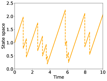
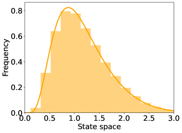
Figure 1: Simulated trajectory from the TCP model with parameter $\kappa=0.4$ until time $10$ (left) and its empirical distribution (in continuous time) evaluated from the first $10\,000$ jumps together with its theoretical version $\mu^{\text{\tiny CT}}$ overlaid (right).

As noted in Remark 2.1, in this model, variance $\sigma_{{\color[rgb]{0.8671875,0.62890625,0.8671875}\text{\footnotesize$\clubsuit$}}}^{2}(x)$ is smaller than variance $\sigma_{{\color[rgb]{0.5,0,0.5}\text{\footnotesize$\vardiamondsuit$}}}^{2}(x)$ by a factor of $\kappa$, uniformly in $x$. These two variances are compared to variance $\sigma_{{\color[rgb]{0.1171875,0.56640625,1}\text{\footnotesize$\spadesuit$}}}^{2}(x)$ (given in Theorem 1.1) for different values of $\kappa$ in Figure 2. This is a numerical evaluation based on formula (9) (together with $\mu^{-}(x)=\kappa\mu(\kappa x)$) without any random generation. This comparison illustrates that, within the same model, the variances intersect, showing that, at least by this criterion, none of the techniques is uniformly superior to the others. However, this comparison criterion does not account for the bias of the estimators or the rate of convergence in the central limit theorems as mentioned in Remark 2.2. For the rest of the simulation study, we restrict ourselves to $\kappa=0.4$ for which $\sigma_{{\color[rgb]{0.1171875,0.56640625,1}\text{\footnotesize$\spadesuit$}}}^{2}(x)$ intersects $\sigma_{{\color[rgb]{0.8671875,0.62890625,0.8671875}\text{\footnotesize$\clubsuit$}}}^{2}(x)$ around $x=2$ and $\sigma_{{\color[rgb]{0.5,0,0.5}\text{\footnotesize$\vardiamondsuit$}}}^{2}(x)$ around $x=2.5$.

$\kappa=0.3$	$\kappa=0.4$	$\kappa=0.5$
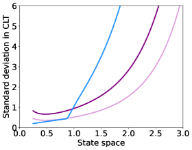
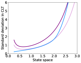
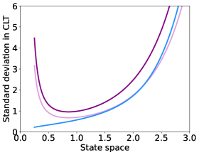
$\kappa=0.6$	$\kappa=0.7$	$\kappa=0.8$

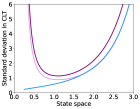
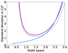
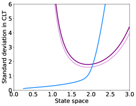
Figure 2: Standard deviations $\sqrt{\sigma_{{\color[rgb]{0.8671875,0.62890625,0.8671875}\text{\footnotesize$\clubsuit$}}}^{2}(x)}$ in pink, $\sqrt{\sigma_{{\color[rgb]{0.5,0,0.5}\text{\footnotesize$\vardiamondsuit$}}}^{2}(x)}$ in purple and $\sqrt{\sigma_{{\color[rgb]{0.1171875,0.56640625,1}\text{\footnotesize$\spadesuit$}}}^{2}(x)}$ in light blue (given in Theorems 1.1 and 2.2) for the TCP model with different values of $\kappa$.

3.2 Bandwidth selection

Kernel methods are highly sensitive to the smoothing parameter, which must therefore be chosen carefully. The estimators under consideration rely on estimating different invariant measures. For instance, $\widehat{\lambda}_{n}^{{\color[rgb]{0.5,0,0.5}\text{\footnotesize$\vardiamondsuit$}}}$ involves estimating $\mu^{-}$, whereas $\widehat{\lambda}_{n}^{{\color[rgb]{0.8671875,0.62890625,0.8671875}\text{\footnotesize$\clubsuit$}}}$ relies on estimating $\mu$. Consequently, there is no reason for them to share the same bandwidth. Moreover, there is no a priori justification for selecting the bandwidth independently for the kernel component of the jump rate estimator; instead, it should be based on the overall formula of the estimator. Additionally, developing a method for adjusting the smoothing bandwidth is a challenging and interesting question that goes far beyond the scope of this paper. Here, we propose a bandwidth selection procedure for each of the estimators based on our knowledge of the ground truth, which, therefore, can not be applied in practice to real-world data.

For the estimator $\widehat{\lambda}$, the smoothing parameter selected in this simulation study is the minimizer of the integrated square error

$$\int_{0.5}^{2.5}\left[\widehat{\lambda}(x)-\lambda(x)\right]^{2}\mathrm{d}x,$$

where the integral is evaluated with a step of $0.05$ and the numerical minimization is performed with a step of $0.025$ for $\widehat{\lambda}_{n}^{{\color[rgb]{0.8671875,0.62890625,0.8671875}\text{\footnotesize$\clubsuit$}}}$ and $\widehat{\lambda}_{n}^{{\color[rgb]{0.5,0,0.5}\text{\footnotesize$\vardiamondsuit$}}}$ and a step of $0.01$ in space and of $0.05$ in time for $\mathring{\lambda}_{n}^{{\color[rgb]{0.1171875,0.56640625,1}\text{\footnotesize$\spadesuit$}}}$ and $\widehat{\lambda}_{n}^{{\color[rgb]{0,0,0.8046875}\text{\footnotesize$\spadesuit$}}}$. Indeed, it should be noted that the latter two estimators, given in (7) and (8), depend on two bandwidths, in space and in time. In addition, the optimal argument selection in $\widehat{\lambda}_{n}^{{\color[rgb]{0,0,0.8046875}\text{\footnotesize$\spadesuit$}}}$ is operated with the same spatial bandwidth as the one used to compute the estimator. Figure 3 presents the results obtained over $100$ replicates for the four estimators from two different sample sizes.

$n=1\,000$


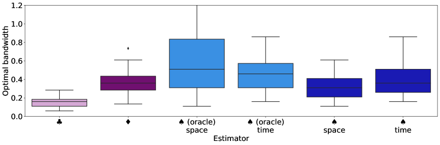
$n=10\,000$

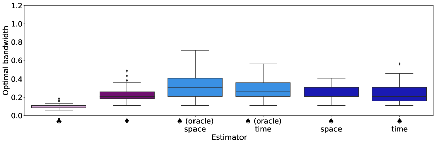
Figure 3: Boxplots over $100$ replicates of smoothing bandwidths minimizing the integrated square error for the four estimators $\widehat{\lambda}_{n}^{{\color[rgb]{0.8671875,0.62890625,0.8671875}\text{\footnotesize$\clubsuit$}}}$ in pink, $\widehat{\lambda}_{n}^{{\color[rgb]{0.5,0,0.5}\text{\footnotesize$\vardiamondsuit$}}}$ in purple, $\mathring{\lambda}_{n}^{{\color[rgb]{0.1171875,0.56640625,1}\text{\footnotesize$\spadesuit$}}}$ in light blue and $\widehat{\lambda}_{n}^{{\color[rgb]{0,0,0.8046875}\text{\footnotesize$\spadesuit$}}}$ in dark blue evaluated from trajectories of size $n=1\,000$ (top) and of size $n=10\,000$ (bottom) generated from the TCP model with parameter $\kappa=0.4$.

The optimal bandwidths vary significantly depending on the estimator used, with a noticeable difference even between estimators $\mathring{\lambda}_{n}^{{\color[rgb]{0.1171875,0.56640625,1}\text{\footnotesize$\spadesuit$}}}$ and $\widehat{\lambda}_{n}^{{\color[rgb]{0,0,0.8046875}\text{\footnotesize$\spadesuit$}}}$, though this difference diminishes with datasets of $10\,000$ observations. Furthermore, as expected, the bandwidths decrease as the number of data points increases. The variability is highest for estimators $\mathring{\lambda}_{n}^{{\color[rgb]{0.1171875,0.56640625,1}\text{\footnotesize$\spadesuit$}}}$ and $\widehat{\lambda}_{n}^{{\color[rgb]{0,0,0.8046875}\text{\footnotesize$\spadesuit$}}}$, where smoothing is applied both to the numerator and the denominator, in both space and time. The variability of the bandwidths for all four estimators also decreases as the dataset size grows. To obtain smoothing parameters that depend only on the type of estimator and the number of available data points (and not on the data themselves), the medians of these empirical distributions are selected. Figure 4 illustrates the behavior of the four estimators evaluated with these optimal bandwidths from a single trajectory.

$n=1\,000$		$n=10\,000$

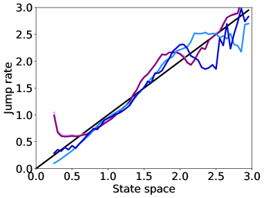
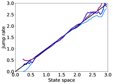
Figure 4: Estimates $\widehat{\lambda}_{n}^{{\color[rgb]{0.8671875,0.62890625,0.8671875}\text{\footnotesize$\clubsuit$}}}(x)$ in pink, $\widehat{\lambda}_{n}^{{\color[rgb]{0.5,0,0.5}\text{\footnotesize$\vardiamondsuit$}}}$ in purple, $\mathring{\lambda}_{n}^{{\color[rgb]{0.1171875,0.56640625,1}\text{\footnotesize$\spadesuit$}}}(x)$ in light blue and $\widehat{\lambda}_{n}^{{\color[rgb]{0,0,0.8046875}\text{\footnotesize$\spadesuit$}}}(x)$ in dark blue computed with the optimal bandwidths (medians of boxplots of Figure 3) from a single trajectory of size $n=1\,000$ (left) and $n=10\,000$ (right) generated from the TCP model with $\kappa=0.4$. The referenced jump rate is given in black line.

3.3 Asymptotic variances vs. estimation errors

The task now is to compare the asymptotic variances of the estimators while taking into account the rate of convergence in the central limit theorem. It should be noted that this can not be done for estimator $\widehat{\lambda}_{n}^{{\color[rgb]{0,0,0.8046875}\text{\footnotesize$\spadesuit$}}}$, for which asymptotic normality has not been theoretically established. According to Theorems 1.1 and 2.2, and as mentioned in Remark 2.2, the pointwise variance in the estimation of $\lambda(x)$ that we expect to observe is normalized by the rate of convergence and thus of the order $\sigma_{{\color[rgb]{0.8671875,0.62890625,0.8671875}\text{\footnotesize$\clubsuit$}}}^{2}(x)/(nh_{n}^{{\color[rgb]{0.8671875,0.62890625,0.8671875}\text{\footnotesize$\clubsuit$}}})$ for $\widehat{\lambda}_{n}^{{\color[rgb]{0.8671875,0.62890625,0.8671875}\text{\footnotesize$\clubsuit$}}}(x)$, $\sigma_{{\color[rgb]{0.5,0,0.5}\text{\footnotesize$\vardiamondsuit$}}}^{2}(x)/(nh_{n}^{{\color[rgb]{0.5,0,0.5}\text{\footnotesize$\vardiamondsuit$}}})$ for $\widehat{\lambda}_{n}^{{\color[rgb]{0.5,0,0.5}\text{\footnotesize$\vardiamondsuit$}}}(x)$ and $\sigma_{{\color[rgb]{0.1171875,0.56640625,1}\text{\footnotesize$\spadesuit$}}}^{2}(x)/(nh_{n}^{{\color[rgb]{0.1171875,0.56640625,1}\text{\footnotesize$\spadesuit$}}\textrm{\tiny s}}h_{n}^{{\color[rgb]{0.1171875,0.56640625,1}\text{\footnotesize$\spadesuit$}}\textrm{\tiny t}})$, where $h_{n}^{{\color[rgb]{0.8671875,0.62890625,0.8671875}\text{\footnotesize$\clubsuit$}}}$, $h_{n}^{{\color[rgb]{0.5,0,0.5}\text{\footnotesize$\vardiamondsuit$}}}$, $h_{n}^{{\color[rgb]{0.1171875,0.56640625,1}\text{\footnotesize$\spadesuit$}}\textrm{\tiny s}}$ and $h_{n}^{{\color[rgb]{0.1171875,0.56640625,1}\text{\footnotesize$\spadesuit$}}\textrm{\tiny t}}$ are the optimal bandwidths selected above (as medians of boxplots of Figure 3). Figure 5 illustrates the asymptotic normality at $x=2$.

$n=1\,000$
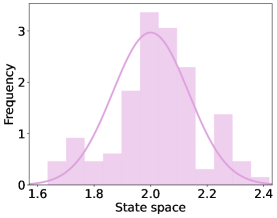
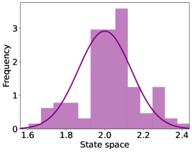
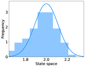
$\clubsuit$	$\vardiamondsuit$	$\spadesuit$ (oracle)
$n=10\,000$
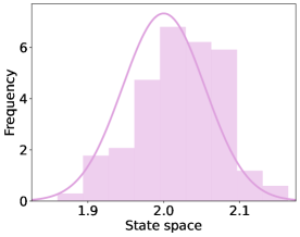
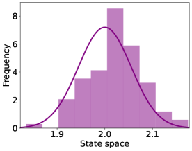
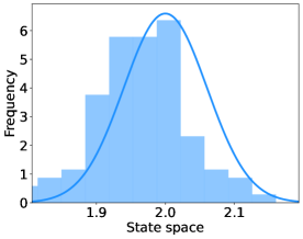
$\clubsuit$	$\vardiamondsuit$	$\spadesuit$ (oracle)

Figure 5: Distribution over $100$ replicates of $\widehat{\lambda}_{n}^{{\color[rgb]{0.8671875,0.62890625,0.8671875}\text{\footnotesize$\clubsuit$}}}(2)$ in pink (left), $\widehat{\lambda}_{n}^{{\color[rgb]{0.5,0,0.5}\text{\footnotesize$\vardiamondsuit$}}}(2)$ in purple (center) and $\mathring{\lambda}_{n}^{{\color[rgb]{0.1171875,0.56640625,1}\text{\footnotesize$\spadesuit$}}}(2)$ in light blue (right) evaluated with optimal bandwidth parameters $h_{n}^{{\color[rgb]{0.8671875,0.62890625,0.8671875}\text{\footnotesize$\clubsuit$}}}$, $h_{n}^{{\color[rgb]{0.5,0,0.5}\text{\footnotesize$\vardiamondsuit$}}}$, $h_{n}^{{\color[rgb]{0.1171875,0.56640625,1}\text{\footnotesize$\spadesuit$}}\textrm{\tiny s}}$ and $h_{n}^{{\color[rgb]{0.1171875,0.56640625,1}\text{\footnotesize$\spadesuit$}}\textrm{\tiny t}}$, from trajectories of size $n=1\,000$ (top) and of size $n=10\,000$ (bottom) generated from the TCP model with parameter $\kappa=0.4$, and referenced Gaussian distributions with mean $\lambda(2)=2$ and variance $\sigma_{{\color[rgb]{0.8671875,0.62890625,0.8671875}\text{\footnotesize$\clubsuit$}}}^{2}(x)/(nh_{n}^{{\color[rgb]{0.8671875,0.62890625,0.8671875}\text{\footnotesize$\clubsuit$}}})$ in pink line (left), with variance $\sigma_{{\color[rgb]{0.5,0,0.5}\text{\footnotesize$\vardiamondsuit$}}}^{2}(x)/(nh_{n}^{{\color[rgb]{0.5,0,0.5}\text{\footnotesize$\vardiamondsuit$}}})$ in purple line (center), and with variance $\sigma_{{\color[rgb]{0.1171875,0.56640625,1}\text{\footnotesize$\spadesuit$}}}^{2}(x)/(nh_{n}^{{\color[rgb]{0.1171875,0.56640625,1}\text{\footnotesize$\spadesuit$}}\textrm{\tiny s}}h_{n}^{{\color[rgb]{0.1171875,0.56640625,1}\text{\footnotesize$\spadesuit$}}\textrm{\tiny t}})$ in light blue line (right).

The empirical distributions shown in Figure 5 align reasonably well with the expected theoretical distributions, particularly for trajectories of size $10\,000$. It should be noted that this analysis falls outside the scope of the theorems, as the bandwidths were chosen numerically and do not follow the theoretically prescribed decay scheme. A slight bias is observable when $n=10\,000$, which highlights (as is well-known) that asymptotic variance alone is insufficient to fully characterize the desirable properties of an estimator. Figure 6 presents the three normalized variances across the state space.

$n=1\,000$		$n=10\,000$

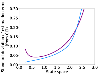
Figure 6: Normalized standard deviations $\sqrt{\sigma_{{\color[rgb]{0.8671875,0.62890625,0.8671875}\text{\footnotesize$\clubsuit$}}}^{2}(x)/(nh_{n}^{{\color[rgb]{0.8671875,0.62890625,0.8671875}\text{\footnotesize$\clubsuit$}}})}$ in pink, $\sqrt{\sigma_{{\color[rgb]{0.5,0,0.5}\text{\footnotesize$\vardiamondsuit$}}}^{2}(x)/(nh_{n}^{{\color[rgb]{0.5,0,0.5}\text{\footnotesize$\vardiamondsuit$}}})}$ in purple and $\sqrt{\sigma_{{\color[rgb]{0.1171875,0.56640625,1}\text{\footnotesize$\spadesuit$}}}^{2}(x)/(nh_{n}^{{\color[rgb]{0.1171875,0.56640625,1}\text{\footnotesize$\spadesuit$}}\textrm{\tiny s}}h_{n}^{{\color[rgb]{0.1171875,0.56640625,1}\text{\footnotesize$\spadesuit$}}\textrm{\tiny t}})}$ in light blue (where $h_{n}^{{\color[rgb]{0.8671875,0.62890625,0.8671875}\text{\footnotesize$\clubsuit$}}}$, $h_{n}^{{\color[rgb]{0.5,0,0.5}\text{\footnotesize$\vardiamondsuit$}}}$, $h_{n}^{{\color[rgb]{0.1171875,0.56640625,1}\text{\footnotesize$\spadesuit$}}\textrm{\tiny s}}$ and $h_{n}^{{\color[rgb]{0.1171875,0.56640625,1}\text{\footnotesize$\spadesuit$}}\textrm{\tiny t}}$ are the bandwidths selected as medians of boxplots of Figure 3) in the TCP model with parameter $\kappa=0.4$, and with $n=1\,000$ (left) and $n=10\,000$ (right).

The normalized variances in Figure 6 show that the two estimators $\widehat{\lambda}_{n}^{{\color[rgb]{0.8671875,0.62890625,0.8671875}\text{\footnotesize$\clubsuit$}}}$ and $\widehat{\lambda}_{n}^{{\color[rgb]{0.5,0,0.5}\text{\footnotesize$\vardiamondsuit$}}}$ behave very similarly, as was already apparent in the example in Figure 4. Moreover, despite having a slower rate of convergence, the normalized variance of estimator $\mathring{\lambda}_{n}^{{\color[rgb]{0.1171875,0.56640625,1}\text{\footnotesize$\spadesuit$}}}$ remains better than the other two for certain regions of the state space: specifically, before approximately $x=2.25$ for $n=1\,000$ and before $x=1$ for $n=10\,000$.

These results suggest that oracle estimator $\mathring{\lambda}_{n}^{{\color[rgb]{0.1171875,0.56640625,1}\text{\footnotesize$\spadesuit$}}}$, and consequently estimator $\widehat{\lambda}_{n}^{{\color[rgb]{0,0,0.8046875}\text{\footnotesize$\spadesuit$}}}$ (assuming their behaviors are expected to be similar), should perform better than the other two on the left side of the state space, and conversely on the right, with a boundary around $x=2.25$ for $n=1\,000$ and $x=1$ for $n=10\,000$. However, this prediction does not account for the estimators’ bias, the potential differences in behavior between estimators $\mathring{\lambda}_{n}^{{\color[rgb]{0.1171875,0.56640625,1}\text{\footnotesize$\spadesuit$}}}$ and $\widehat{\lambda}_{n}^{{\color[rgb]{0,0,0.8046875}\text{\footnotesize$\spadesuit$}}}$, or the gap between theoretical results and the setup of numerical simulations. We now aim to assess the accuracy of this prediction. To this end, we evaluated over $100$ replicates the pointwise estimation error $|\widehat{\lambda}(x)-\lambda(x)|$ across the state space for the four estimators under consideration. Results are given in Figure 7.

$n=1\,000$


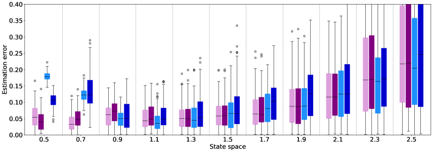
$n=10\,000$

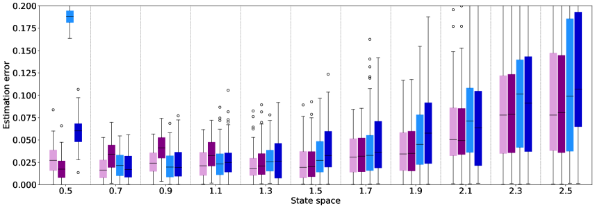
Figure 7: Pointwise estimation error over $100$ replicates for the four estimators $\widehat{\lambda}_{n}^{{\color[rgb]{0.8671875,0.62890625,0.8671875}\text{\footnotesize$\clubsuit$}}}(x)$ in pink, $\widehat{\lambda}_{n}^{{\color[rgb]{0.5,0,0.5}\text{\footnotesize$\vardiamondsuit$}}}(x)$ in purple, $\mathring{\lambda}_{n}^{{\color[rgb]{0.1171875,0.56640625,1}\text{\footnotesize$\spadesuit$}}}(x)$ in light blue and $\widehat{\lambda}_{n}^{{\color[rgb]{0,0,0.8046875}\text{\footnotesize$\spadesuit$}}}(x)$ in dark blue, from left to right for each value of $x$ (with $x$ between $0.5$ and $2.5$ with a step of $0.2$), computed from a trajectory of size $n=1\,000$ (top) and of size $n=10\,000$ (bottom).

The general pattern of variability aligns fairly well with the theoretical predictions from Figure 6. However, in addition to exhibiting increasing variance, all four estimators appear to suffer from a bias toward the right side of the state space ($x>2$), regardless of the sample size. On the left side of the state space ($x<1$), only estimators $\mathring{\lambda}_{n}^{{\color[rgb]{0.1171875,0.56640625,1}\text{\footnotesize$\spadesuit$}}}$ and $\widehat{\lambda}_{n}^{{\color[rgb]{0,0,0.8046875}\text{\footnotesize$\spadesuit$}}}$ experience significant bias, along with greatly reduced variance (as predicted by theory). In the central and right parts of the state space ($x>1$), all four estimators display very similar behavior, with estimator $\widehat{\lambda}_{n}^{{\color[rgb]{0.8671875,0.62890625,0.8671875}\text{\footnotesize$\clubsuit$}}}$ having a nearly uniform advantage.

Before delving into details, we exclude estimator $\widehat{\lambda}_{n}^{{\color[rgb]{0.8671875,0.62890625,0.8671875}\text{\footnotesize$\clubsuit$}}}$, which uses the form of the transition kernel, and the oracle estimator $\mathring{\lambda}_{n}^{{\color[rgb]{0.1171875,0.56640625,1}\text{\footnotesize$\spadesuit$}}}$, whose argument selection relies on the invariant law of the process. This leaves us comparing estimators $\widehat{\lambda}_{n}^{{\color[rgb]{0.5,0,0.5}\text{\footnotesize$\vardiamondsuit$}}}$ and $\widehat{\lambda}_{n}^{{\color[rgb]{0,0,0.8046875}\text{\footnotesize$\spadesuit$}}}$, which are based on exactly the same data. In this comparison, aside from the bias suffered by $\widehat{\lambda}_{n}^{{\color[rgb]{0,0,0.8046875}\text{\footnotesize$\spadesuit$}}}$ on the left side of the state space, the theoretical predictions are generally supported by the numerical simulations, especially from trajectories of size $n=10\,000$: for $0.7\leq x\leq 1.1$, $\widehat{\lambda}_{n}^{{\color[rgb]{0,0,0.8046875}\text{\footnotesize$\spadesuit$}}}(x)$ performs better than $\widehat{\lambda}_{n}^{{\color[rgb]{0.5,0,0.5}\text{\footnotesize$\vardiamondsuit$}}}(x)$, while for $x\geq 1.3$, the situation reverses.

While the previously mentioned limitations of applying theoretical results in this context remain valid (and are particularly evident when comparing the four estimators in detail), they nonetheless allow for a reasonably reliable comparison of the two main estimators studied. Moreover, the numerical analysis confirms, using the TCP model as an example, that none of the methods is uniformly better across the state space.

4 Real data analysis

4.1 Context

The life cycle of a cell alternates phases of growth and division. This is a typical application of piecewise-deterministic models in dimension 1 (see for instance [8, 13, 19] and references therein): growth is considered exponential and divisions, assumed to be quasi-instantaneous, occur at random times. In addition, the division mechanism appears to be linked to cell size [22], making the idea of a jump rate as a function of cell size relevant. In this context, the process under consideration models the size of a cell (and its progeny) over time: its flow is of the form $(x,t)\mapsto x\exp(\theta t)$, $\theta>0$, and its transition kernel can be written as $\delta_{\{x/2\}}$ (or more generally as any distribution with support $[0,x]$ to take into account both the intrinsic variability and an eventual bias in the division process). The jump rate, which is very difficult to parameterize in this kind of application, is the typical function of interest.

In this section, we propose to use single-cell data from Escherichia coli [23] to implement and compare, within the framework of the probabilistic model just described, the jump rate estimation strategies studied in this paper. The data in question are measurements of cell size, obtained by microscopy, under different temperature conditions (25°C, 27°C, or 37°C). For each, multiple independent data sets from different mother cells are available.

In Subsection 4.2, we describe the available data and explain how a piecewise-deterministic model is fitted to them. The results of the jump rate estimation for the three temperature conditions are presented in Subsection 4.3.

4.2 Data description and model fitting

Whatever the temperature condition, the data of interest are organized in different files corresponding to independent cell lineages. For each, cell size is measured every minute. In addition, a division indicator is available which, in a piecewise-deterministic model, precisely indicates the jump times. Consequently, the observation scheme chosen in the paper is precisely that of these data. Table 1 provides information on the sample sizes available under each of the temperature conditions, while Figure 8 shows some of the process statistics. We can already see that the behavior of the process appears to be strongly temperature-dependent.

Temperature		Lineages	Measurements	Division events
25°C	Total:	65	307 999	4 485
	Average (per lineage):	—	4738.44	68.67
27°C	Total:	54	202 086	3 726
	Average (per lineage):	—	3742.33	69
37°C	Total:	160	364 920	11 040
	Average (per lineage):	—	2280.75	69

Table 1: Summary of growth data under each of the temperature conditions.

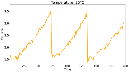
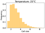
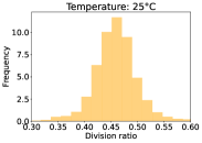
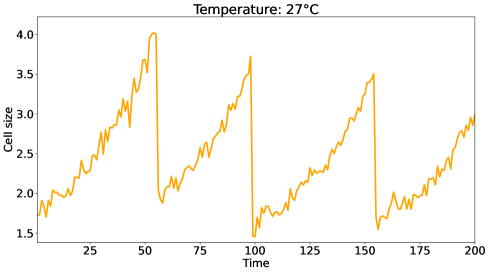
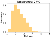
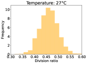
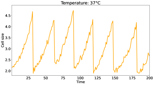
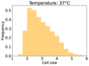
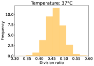
Figure 8: Under each of the temperature conditions (upper panel: 25°C, centered panel: 27°C, lower panel: 37°C), cell size measurements (unit of size is micrometer) until time 200 (unit of time is minute) from lineage xy01_02 (left), distribution of cell size from $10\,000$ consecutive measurements (mixing different lineages) (top right), and distribution of division ratio (bottom right).

We now turn our attention to piecewise-deterministic Markov process modeling in order to apply the statistical procedures studied in this article. Looking at the empirical law of division ratios in Figure 8, we are convinced that, whatever the temperature experiment, the transition kernel can not be modeled by a Dirac mass, which rules out Krell’s approach. That leaves us with the question of how to model the flow. For this, we assume exponential cell growth mentioned above, and model the logarithm of cell size by a linear function, i.e. $\Phi(t|x)=x+\theta t$. To obtain a one-dimensional model, $\theta$ must not depend on any quantity (except perhaps the temperature condition which is expected to play a significant role), especially on the cell in question. For each of the temperature condition, for each of the thousands of cells along the hundreds of lineages measured, we fit a linear model to their growth. Some results, gathered by temperature condition, are given in Figure 9. We observe that the histogram of estimated slopes depends on the temperature but is always unimodal with very low variance. We therefore accept the constant (but temperature-dependent) slope hypothesis and take for $\theta$ its mean value: $\theta=0.012$ at 25°C, $\theta=0.014$ at 27°C, and $\theta=0.025$ at 37°C. Figure 9 also illustrates the quality of the piecewise-linear fit to the data.

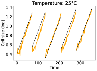
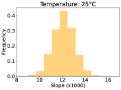
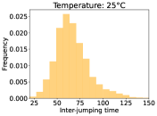
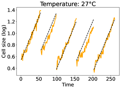
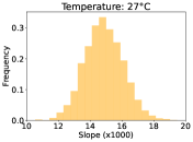
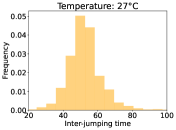
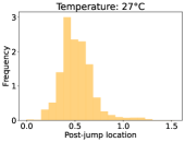
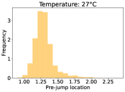
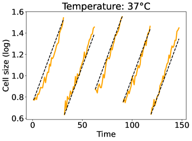
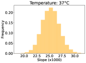
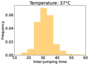
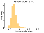
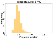
Figure 9: Under each of the temperature conditions (upper panel: 25°C, centered panel: 27°C, lower panel: 37°C), logarithm of cell size measurements before the fifth division event and fitted linear growth (left), distribution of estimated slope (top center), distribution of time between two consecutive division events (bottom center), distribution of logarithm of cell size at division time (top right), and distribution of logarithm of cell size just before division (bottom right).

4.3 Jump rate estimation

Now that the model has been fitted, we can calculate the estimators of the jump rate. Estimator $\widehat{\lambda}_{n}^{{\color[rgb]{0.5,0,0.5}\text{\footnotesize$\vardiamondsuit$}}}$ only requires the evaluation of $\Delta$ (the derivative of the inverse of the flow), which here is simply a constant equal to $\theta^{-1}$. To calculate estimator $\widehat{\lambda}_{n}^{{\color[rgb]{0,0,0.8046875}\text{\footnotesize$\spadesuit$}}}$, we simplify the procedure from [5]. As can be seen from Figure 9, the process of interest is rather stereotyped, with empirical distributions of the embedded Markov chain quite concentrated around their mode. For instance, inter-jumping times are mainly around $\tau=31.6$ on average at 37°C ($\tau=66.6$ at 25°C and $\tau=52.4$ at 27°C). To estimate $\lambda(x)$, we therefore skip the complex step of optimal argument selection and evaluate the estimator at $(\xi,\tau)$ where $\xi=x-\theta\tau$ so that $\Phi(\tau|\xi)=x$.

The final step is to select the smoothing parameters. In the absence of ground truth, these are chosen by hand to avoid over-fitting (resulting in excessive oscillations) and under-fitting (no apparent variation). We also use our knowledge from numerical simulations: spatial bandwidths of the two estimators are very close. In addition, both bandwidths are expected to decrease in the sample size. Selected parameters are given in Table 2.

Temperature	Sample size	$\vardiamondsuit$ bandwidth	$\spadesuit$ bandwidth (space)	$\spadesuit$ bandwidth (time)
25°C	4 485	0.05	0.06	4
27°C	3 726	0.07	0.08	8
37°C	11 040	0.02	0.03	3

Table 2: Summary of bandwidth parameters for $\widehat{\lambda}_{n}^{{\color[rgb]{0.5,0,0.5}\text{\footnotesize$\vardiamondsuit$}}}$ and $\widehat{\lambda}_{n}^{{\color[rgb]{0,0,0.8046875}\text{\footnotesize$\spadesuit$}}}$ (space and time) under each of the temperature conditions.

Estimation results are given in Figure 10. To help with interpretation, we represent the function of cell size $x\mapsto\lambda(\exp(x))$. Both methods show that the behavior of the jump rate depends strongly on the temperature of the experiment, as expected. The two estimators are qualitatively comparable, but differ when viewed in detail. For example, growth in the jump rate starts earlier for $\widehat{\lambda}_{n}^{{\color[rgb]{0,0,0.8046875}\text{\footnotesize$\spadesuit$}}}$ than for $\widehat{\lambda}_{n}^{{\color[rgb]{0.5,0,0.5}\text{\footnotesize$\vardiamondsuit$}}}$, whatever the temperature condition. This analysis also highlighted the high sensitivity of $\widehat{\lambda}_{n}^{{\color[rgb]{0,0,0.8046875}\text{\footnotesize$\spadesuit$}}}$ to smoothing parameters, particularly for the smallest samples, making it a more difficult method to calibrate.

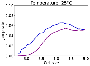
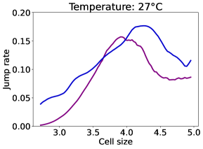
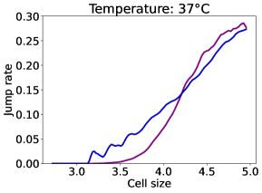
Figure 10: Estimated jump rates as a function of cell size using $\widehat{\lambda}_{n}^{{\color[rgb]{0.5,0,0.5}\text{\footnotesize$\vardiamondsuit$}}}$ (purple) and $\widehat{\lambda}_{n}^{{\color[rgb]{0,0,0.8046875}\text{\footnotesize$\spadesuit$}}}$ (dark blue) under different temperature conditions.

5 Concluding remarks

Non-parametric estimation of the jump rate of PDMPs requires the development of specific methods. In dimension 1, the state of the art is limited to five main approaches [4, 5, 16, 18, 20] that address the function of interest in different ways. In the first part of the article, we highlighted connections between three of them [16, 18, 20] that had not been noticed in the literature. In particular, the approaches of Fujii [16] and Krell and Schmisser [20] are implicitly based on the same formula (4) to tackle the jump rate of interest. It is important to note that the statistical techniques and subsequent results in these two papers are nevertheless different and complementary. The main difference between these approaches [16, 20] and that of Krell lies in the estimation of the invariant distribution of pre-jump locations, captured in [18] via post-jump locations using the additional assumption of deterministic transitions.

That being said, we find it important to further investigate the comparison of these approaches. While they all construct consistent estimators of the jump rate without imposing strong assumptions on the model’s form, a natural question arises: can they be distinguished at a higher order, for instance, through their convergence rate or asymptotic variance? This question was difficult to address given the different theoretical frameworks of the reference papers. Consequently, we proposed to standardize these approaches, notably by restricting ourselves to non-recursive kernel methods. The approach based on the multiplicative intensity model [4] was set aside, primarily because it does not provide a direct estimator of the jump rate. However, we believe this method warrants further investigation and should be considered in a broader comparative analysis. Nonetheless, this lies beyond the scope of the present work.

In order to theoretically compare the inference methods in question, we have shown new results of consistency and asymptotic normality for the standardized versions of the estimators of Krell [18] and of Fujii and Krell and Schmisser [16, 20], making them comparable with Azaïs and Muller-Gueudin’s approach [5]. The proof involves the study of vector martingales constructed along the embedded chain of the PDMP. The theoretical results prove that the three standardized estimators can not in general be ordered based on their asymptotic variance, even within the same model. This result is surprising for two main reasons: (i) the estimator based on [18] is the only one that leverages the deterministic nature of the transitions, which does not guarantee that it achieves the lowest variance everywhere; (ii) the technique based on [5] does not exploit the one-dimensional nature of the state space (as it was developed to operate in any dimension), which does not prevent it from achieving the lowest variance in certain regions of the state space.

We have demonstrated that these theoretical results align with numerical simulations in the context of the TCP model, a representative application of PDMPs in dimension 1. However, the numerical experiments also highlight the greater sensitivity of the estimator proposed by Azaïs and Muller-Gueudin [5] to the choice of smoothing parameters. Unlike the other two methods (which involve smoothing only in space), this approach requires smoothing in both space and time, as well as an optimal argument selection, making it the most complex technique to implement. The application to real data confirms this trend, underscoring the practical advantages of the approach based on Fujii’s and Krell and Schmisser’s papers [16, 20]. Given the current state of knowledge, their method is likely the most suitable choice in dimension 1, despite exhibiting higher variance in certain cases.

The most promising solution is likely to involve aggregating the estimators studied in the present paper to leverage the strengths of each approach. For example, a compelling direction suggested by our analysis would be to select, at each point in the state space, the estimator with the lowest asymptotic variance.

Appendix A Proof of the main results

The goal of this appendix is to prove the consistency (given in Theorem 2.1) and the asymptotic normality (given in Theorem 2.2) of jump rate estimators under consideration. The proof is given in detail below for estimator $\widehat{\lambda}_{n}^{{\color[rgb]{0.8671875,0.62890625,0.8671875}\text{\footnotesize$\clubsuit$}}}(x)$. The proof for $\widehat{\lambda}_{n}^{{\color[rgb]{0.5,0,0.5}\text{\footnotesize$\vardiamondsuit$}}}(x)$ follows exactly the same reasoning and is omitted for brevity.

A.1 Sketch of the proof

The proof relies on the following formula (stated in Remark 1.2) for the jump rate,

$$\lambda(x)=\frac{\mu(h(x))}{D(x)},$$

where

$$D(x)=\frac{\mathbb{P}_{\mu}\left(Z_{0}\leq x,Z_{1}\geq h(x)\right)}{h^{\prime}(x)\Delta(x)}.$$ (10)

The numerator and the denominator are estimated by

$$\widehat{\mu}_{n}(h(x)) = \frac{1}{n}\sum_{i=1}^{n}K_{h_{n}}(Z_{i}-h(x)),$$

$$\widehat{D}_{n}(x) = \frac{1}{nh^{\prime}(x)\Delta(x)}\sum_{i=1}^{n}\mathbbm{1}_{\{Z_{i-1}\leq x\}}\mathbbm{1}_{\{Z_{i}\geq h(x)\}},$$

where $h_{n}=cn^{-\gamma}$, $1/3<\gamma<1$ (for the sake of readability, $c=1$ in the sequel of the proof). $\widehat{\lambda}_{n}^{{\color[rgb]{0.8671875,0.62890625,0.8671875}\text{\footnotesize$\clubsuit$}}}(x)$ is basically the quotient of $\widehat{\mu}_{n}(h(x))$ over $\widehat{D}_{n}(x)$. In order to establish the asymptotic properties of $\widehat{\lambda}_{n}^{{\color[rgb]{0.8671875,0.62890625,0.8671875}\text{\footnotesize$\clubsuit$}}}(x)$, we shall study the vector $(\widehat{\mu}_{n}(h(x)),\widehat{D}_{n}(x))^{\top}$. Our main goal is to show that this vector tends to its deterministic counterpart, $(\mu(h(x)),D(x))^{\top}$, and catch the rate of convergence.

To this end, we introduce the following pieces of notation. First, $F_{n}$ denotes the $\sigma$-algebra generated by $Z_{0},\dots,Z_{n}$. $M_{n}=(M_{n}^{(1)},M_{n}^{(2)})^{\top}$ is the vector martingale (adapted to $F_{n}$) defined by,

$$\forall\,i\in\{1,2\},~M_{n}^{(i)}=\sum_{k=1}^{n}\left(A_{k}^{(i)}-B_{k}^{(i)}\right),$$ (11)

where

$$A_{k}^{(1)} = K_{h_{n}}\left(Z_{k}-h(x)\right),$$

$$A_{k}^{(2)} = \frac{\mathbbm{1}_{\{Z_{k}\geq h(x),x\geq Z_{k-1}\}}}{h^{\prime}(x)\Delta(x)},$$

$$\forall\,i\in\{1,2\},~B_{k}^{(i)} = \mathbb{E}[A_{k}^{(i)}|F_{k-1}].$$

We also consider $R_{n}=(R_{n}^{(1)},R_{n}^{(2)})^{\top}$ defined by

$$R_{n}^{(1)} = \frac{1}{n}\sum_{k=1}^{n}B_{k}^{(1)}-\mu(h(x)),$$

$$R_{n}^{(2)} = \frac{1}{n}\sum_{k=1}^{n}B_{k}^{(2)}-D(x).$$

Then a direct calculus shows that the two-dimensional estimation error is given by

$$\left(\begin{matrix}\widehat{\mu}_{n}(h(x))\\ \widehat{D}_{n}(x)\end{matrix}\right)-\left(\begin{matrix}\mu(h(x))\\ D(x)\end{matrix}\right)=\frac{M_{n}}{n}+R_{n}.$$ (12)

This decomposition is at the core of our demonstration. In Appendix A.3, we establish that $M_{n}/n$ almost surely goes to $0$ by virtue of the law of large numbers for vector martingales, and state that the remainder term $R_{n}$ also vanishes, establishing the consistency of $\widehat{\lambda}_{n}^{{\color[rgb]{0.8671875,0.62890625,0.8671875}\text{\footnotesize$\clubsuit$}}}(x)$ given in Theorem 2.1. In Appendix A.4, we first state that $n^{(1-\gamma)/2}R_{n}$ goes to $0$ in probability. The convergence of the estimation error is therefore carried by the martingale term, which we study in light of the central limit theorem for vector martingales. This will prove the asymptotic normality of $\widehat{\lambda}_{n}^{{\color[rgb]{0.8671875,0.62890625,0.8671875}\text{\footnotesize$\clubsuit$}}}(x)$ given in Theorem 2.2. Before that, we investigate the predictable square variation process of $M_{n}$ in Appendix A.2.

A.2 Square variation process

The predictable square variation process of $M_{n}$ is given by

$$\left\langle M\right\rangle_{n}=\sum_{k=1}^{n}\left(\mathbb{E}\left[M_{k}^{\top}M_{k}|F_{k-1}\right]-M_{k-1}^{\top}M_{k-1}\right).$$

In this section we aim to establish the following lemma that describes the asymptotic behavior of $\left\langle M\right\rangle_{n}$.

Lemma A.1.

When $n$ goes to infinity, the following equality holds almost surely,

$$\left\langle M\right\rangle_{n}=\left[\begin{matrix}n^{1+\gamma}\omega_{1}(1+o(1))&O(n)\\ O(n)&n\omega_{2}(1+o(1))\end{matrix}\right],$$

where $\omega_{1}$ and $\omega_{2}$ are positive numbers.

Proof.

We analyze the coefficients of the matrix separately.

$\bullet$ Study of $\left\langle M\right\rangle_{n}^{(1,1)}$

A direct calculus shows that

$$\left\langle M\right\rangle_{n}^{(1,1)} = \sum_{k=1}^{n}\mathbb{V}\textrm{ar}(M_{k}^{(1)}|F_{k-1})$$

$$= \sum_{k=1}^{n}\mathbb{V}\textrm{ar}\left(\sum_{j=1}^{k}(A_{j}^{(1)}-B_{j}^{(1)})\Big{|}F_{k-1}\right)$$

$$= \sum_{k=1}^{n}\left(\mathbb{E}\left[(A_{k}^{(1)})^{2}\big{|}F_{k-1}\right]-\mathbb{E}\left[A_{k}^{(1)}\big{|}F_{k-1}\right]^{2}\right).$$

Recalling that $P$ is the conditional density of $Z_{k}$ given $Z_{k-1}$, with a change of variable, one has

$$\mathbb{E}\left[(A_{k}^{(1)})^{2}\big{|}F_{k-1}\right] = \frac{1}{h_{n}}\int_{\mathbb{R}}K^{2}\left(u\right)P(h_{n}u+h(y)|Z_{k-1})\mathrm{d}u,$$

$$\mathbb{E}\left[A_{k}^{(1)}\big{|}F_{k-1}\right]^{2} = \left(\int_{\mathbb{R}}K\left(u\right)P(h_{n}u+h(y)|Z_{k-1})\mathrm{d}u\right)^{2}.$$

This yields

$$\left\langle M\right\rangle_{n}^{(1,1)}=nT_{n}^{(1)}-T_{n}^{(2)},$$ (13)

where

$$T_{n}^{(1)} = \frac{1}{nh_{n}}\sum_{k=1}^{n}\int_{\mathbb{R}}K^{2}\left(u\right)P(h_{n}u+h(y)|Z_{k-1})\mathrm{d}u,$$

$$T_{n}^{(2)} = \sum_{k=1}^{n}\left(\int_{\mathbb{R}}K\left(u\right)P(h_{n}u+h(y)|Z_{k-1})\mathrm{d}u\right)^{2}.$$

We shall investigate the limit behavior of $T_{n}^{(1)}$ and $T_{n}^{(2)}$. To this end, we define

$$\hat{T}_{n}^{(1)} = \frac{\tau^{2}}{n}\sum_{k=1}^{n}P(h(x)|Z_{k-1}),$$

$$\tilde{T}_{n}^{(1)} = \frac{1}{n}\sum_{k=1}^{n}\int_{\mathbb{R}}K^{2}\left(u\right)P(h_{n}u+h(x)|Z_{k-1})\mathrm{d}u,$$

where $\tau^{2}=\int_{\mathbb{R}}K^{2}(x)\mathrm{d}x$. Using the fact that $P$ is Lipschitz as supposed in Assumptions 2.3 and $K$ has compact support by Assumptions 2.5, one has

$$|\hat{T}_{n}^{(1)}-\tilde{T}_{n}^{(1)}| \leq \frac{1}{n}\sum_{k=1}^{n}\int_{\mathbb{R}}K^{2}(u)\left|P(h_{n}u+h(x)|Z_{k-1})-P(h(x)|Z_{k-1})\right|\mathrm{d}u$$ (14)

$$\leq \frac{[P]_{\text{\tiny Lip}}}{n}\sum_{k=1}^{n}\int_{\mathbb{R}}K^{2}(u)|h_{n}u|\mathrm{d}u$$

$$\leq h_{n}[P]_{\text{\tiny Lip}}\int_{\mathbb{R}}K^{2}(u)|u|\mathrm{d}u~\to 0,$$

when $n$ goes to infinity, because $h_{n}=n^{-\gamma}$. Furthermore, by virtue of the almost sure ergodic theorem [21, Theorem 17.1.7] (which we can apply by Assumption 2.2) and recalling that $\mu$ is the invariant measure of $P$,

$$\hat{T}_{n}^{(1)}\overset{\textrm{a.s.}}{\longrightarrow}\tau^{2}\mathbb{E}_{\mu}[P(h(x)|Z_{0})]=\tau^{2}\mu(h(x)).$$

Since $\hat{T}_{n}^{(1)}$ and $\tilde{T}_{n}^{(1)}$ have the same limit by (14), and writing $T_{n}^{(1)}=\tilde{T}_{n}^{(1)}/h_{n}$, one gets the following almost sure equivalent when $n$ goes to infinity,

$$nT_{n}^{(1)}\sim n^{1+\gamma}\tau^{2}\mu(h(x)).$$ (15)

In addition, since $P$ is bounded according to Assumptions 2.3,

$$T_{n}^{(2)}\leq\|P\|_{\infty}^{2}n.$$

Together with (13) and (15), one gets

$$\frac{\left\langle M\right\rangle_{n}^{(1,1)}}{n^{1+\gamma}}\overset{\textrm{a.s.}}{\longrightarrow}\tau^{2}\mu(h(x)),$$

establishing the expected result for coefficient $\left\langle M\right\rangle_{n}^{(1,1)}$.

$\bullet$ Study of $\left\langle M\right\rangle_{n}^{(2,2)}$

One has

$$\left\langle M\right\rangle_{n}^{(2,2)}=\sum_{k=1}^{n}\mathbb{V}\textrm{ar}(A_{k}^{(2)}|Z_{k-1}).$$

Each term, $\mathbb{V}\textrm{ar}(A_{k}^{(2)}|Z_{k-1})$, of the sum is a function of $Z_{k-1}$ and is independent of $n$. This contrasts with its counterpart, $\mathbb{V}\textrm{ar}(A_{k}^{(1)}|Z_{k-1})$, in $\left\langle M\right\rangle_{n}^{(1,1)}$, which exhibits an explicit dependence on $n$. In that context, one can directly apply the almost sure ergodic theorem [21, Theorem 17.1.7] and get

$$\frac{\left\langle M\right\rangle_{n}^{(2,2)}}{n}\overset{\textrm{a.s.}}{\longrightarrow}\frac{1}{h^{\prime}(x)^{2}\Delta(x)^{2}}\int_{\mathbb{R}_{+}}p(y)(1-p(y))\mu(\mathrm{d}y),$$

where

$$p(y)=\mathbb{P}(Z_{0}\leq x<Z_{1}^{-}|Z_{0}=y),$$

stating the expected result for $\left\langle M\right\rangle_{n}^{(2,2)}$.

$\bullet$ Study of $\left\langle M\right\rangle_{n}^{(1,2)}=\left\langle M\right\rangle_{n}^{(2,1)}$

With a change of variable, it is easy to see that both

$$\mathbb{E}[A_{k}^{(1)}A_{k}^{(2)}|Z_{k-1}]$$

and

$$\mathbb{E}[A_{k}^{(1)}|Z_{k-1}]\,\mathbb{E}[A_{k}^{(2)}|Z_{k-1}]$$

are bounded by $\|P\|_{\infty}/(h^{\prime}(x)\Delta(x))$. Together with

$$\left\langle M\right\rangle_{n}^{(1,2)}=\sum_{k=1}^{n}\mathbb{E}[A_{k}^{(1)}A_{k}^{(2)}|Z_{k-1}]-\mathbb{E}[A_{k}^{(1)}|Z_{k-1}]\,\mathbb{E}[A_{k}^{(2)}|Z_{k-1}],$$

this shows that the non-diagonal coefficients are in $O(n)$, as expected. ∎

A.3 Consistency

In light of (12), if the martingale term $M_{n}/n$ and the remainder term $R_{n}$ go to $0$, then $\widehat{\lambda}_{n}^{{\color[rgb]{0.8671875,0.62890625,0.8671875}\text{\footnotesize$\clubsuit$}}}(x)$ is consistent. We tackle the two terms separately.

A.3.1 Remainder term

With a change of variable,

$$R_{n}^{(1)}=\frac{1}{n}\sum_{k=1}^{n}\int_{\mathbb{R}}K\left(u\right)P\left(h_{n}u+h(x)|Z_{k-1}\right)\mathrm{d}u-\mu(h(x)).$$

Then, using $\int_{\mathbb{R}}K(u)\mathrm{d}u=1$ (see Assumptions 2.5),

$$R_{n}^{(1)}=R_{n}^{(1,1)}+R_{n}^{(1,2)},$$ (16)

where

$$R_{n}^{(1,1)} = \frac{1}{n}\sum_{k=1}^{n}\int_{\mathbb{R}}K\left(u\right)\left[P\left(h_{n}u+h(x)|Z_{k-1}\right)-P\left(h(x)|Z_{k-1}\right)\right]\mathrm{d}u,$$

$$R_{n}^{(1,2)} = \frac{1}{n}\sum_{k=1}^{n}P\left(h(x)|Z_{k-1}\right)-\mu(h(x)).$$ (17)

Since $P$ is Lipschitz according to Assumptions 2.3,

$$|R_{n}^{(1,1)}|\leq h_{n}[P]_{\text{\tiny Lip}}\int_{\mathbb{R}}K(u)|u|\mathrm{d}u~\to 0.$$ (18)

In addition, $R_{n}^{(1,2)}$ almost surely vanishes by direct application of the almost sure ergodic theorem [21, Theorem 17.1.7]. This proves that $R_{n}^{(1)}$ tends to $0$. Furthermore,

$$R_{n}^{(2)}=\frac{1}{nh^{\prime}(x)\Delta(x)}\sum_{k=1}^{n}\mathbbm{1}_{\{x\geq Z_{k-1}\}}\mathbb{E}[\mathbbm{1}_{\{Z_{k}\geq h(x)\}}|Z_{k-1}]-D(x),$$

which directly goes to $0$, in light of the almost sure ergodic theorem again, and by definition (10) of $D(x)$.

A.3.2 Martingale term

The submultiplicativity of the Frobenius norm, together with the asymptotic behavior of $\left\langle M\right\rangle_{n}$ stated in Lemma A.1, imply that

$$\frac{\|M_{n}\|^{2}}{n^{2}} = \frac{\|\left\langle M\right\rangle_{n}^{1/2}\left\langle M\right\rangle_{n}^{-1/2}M_{n}\|^{2}}{n^{2}}$$

$$\leq \|\left\langle M\right\rangle_{n}^{-1/2}M_{n}||^{2}n^{\gamma-1}\max(\omega_{1},\omega_{2}).$$

By virtue of the law of large numbers for vector martingales [14, Theorem 1.3.15], for any $\eta>0$, when $n$ goes to infinity,

$$\|\left\langle M\right\rangle_{n}^{-1/2}M_{n}\|^{2}=o\left(\frac{\log(\mathcal{T}_{n})^{1+\eta}}{\mathcal{E}_{n}}\right),$$

where $\mathcal{E}_{n}$ ($\mathcal{T}_{n}$, respectively) denotes the smallest eigenvalue (the trace, respectively) of $\left\langle M\right\rangle_{n}$. By Lemma A.1, it is clear that $\mathcal{T}_{n}=O(n^{1+\gamma})$ and $\mathcal{E}_{n}\sim\omega_{2}n$ almost surely. All together, this establishes that $M_{n}/n$ almost surely vanishes, which ends the proof of the consistency of $\widehat{\lambda}_{n}^{{\color[rgb]{0.8671875,0.62890625,0.8671875}\text{\footnotesize$\clubsuit$}}}(x)$.

A.4 Asymptotic normality

Using (12), we derive a central limit theorem for $\widehat{\lambda}_{n}^{{\color[rgb]{0.8671875,0.62890625,0.8671875}\text{\footnotesize$\clubsuit$}}}(x)$ by proving that the martingale term converges to a Gaussian distribution as the remainder term vanishes.

A.4.1 Remainder term

We begin with $R_{n}^{(1)}$ written as the sum (16) of $R_{n}^{(1,1)}$ and $R_{n}^{(2,2)}$. With (18),

$$n^{(1-\gamma)/2}R_{n}^{(1,1)}\leq n^{(1-3\gamma)/2}[P]_{\text{\tiny Lip}}\int_{\mathbb{R}}K(u)|u|\mathrm{d}u,$$

which goes to $0$ as long as $1/3<\gamma<1$. In addition, by virtue of [14, Theorem 6.3.17] applied to functional $P$ (which satisfies Assumptions 2.3) along Markov chain $Z_{n}$, one has almost surely

$$\left|\sum_{k=0}^{n}\left(P(h(x)|Z_{k})-\mathbb{E}_{\mu}\left[P(h(x)|Z_{0})\right]\right)\right|=o\left((n\ln(n)^{1+\gamma})^{\frac{r_{1}+r_{2}}{a_{1}}}\right).$$

With $\mathbb{E}_{\mu}\left[P(h(x)|Z_{0})\right]=\mu(h(x))$, one gets

$$\left|\frac{1}{n^{\frac{1+\gamma}{2}}}\sum_{k=0}^{n}\left(P(h(x)|Z_{k})-\mu(h(x))\right)\right|=o\left(n^{\frac{r_{1}+r_{2}}{a_{1}}-\frac{1+\gamma}{2}}\ln(n)^{(1+\gamma)\frac{r_{1}+r_{2}}{a_{1}}}\right).$$

Moreover $(r_{1}+r_{2})/a_{1}-(\gamma+1)/2\leq-\gamma/2<0$ because $(r_{1}+r_{2})/a_{1}\leq 1/2$ in light of Assumptions 2.4. Together with the definition (17) of $R_{n}^{(1,2)}$, this shows that $n^{(1-\gamma)/2}R_{n}^{(1,2)}$ almost surely vanishes. As a conclusion, $n^{(1-\gamma)/2}R_{n}^{(1)}$ almost surely goes to $0$.

On the other hand, the central limit theorem for Markov chains [21, Theorem 17.5.3] proves that $\sqrt{n}R_{n}^{(2)}$ weakly converges to a Gaussian distribution with mean $0$ and finite variance. Consequently, $n^{(1-\gamma)/2}R_{n}^{(2)}$ tends to $0$, and

$$n^{(1-\gamma)/2}R_{n}\overset{\mathbb{P}}{\longrightarrow}0.$$ (19)

A.4.2 Martingale term

To establish the asymptotic normality of the martingale term $M_{n}/n$ with rate $n^{(1-\gamma)/2}$, we rely on the central limit theorem for vector martingales [14, Corollary 2.1.10]. To this end, we need to check its conditions of applicability. First, in light of Lemma A.1, it is clear that

$$\frac{\left\langle M\right\rangle_{n}}{n^{1+\gamma}}\overset{\textrm{a.s.}}{\longrightarrow}\left[\begin{matrix}\tau^{2}\mu(h(x))&0\\ 0&0\end{matrix}\right].$$ (20)

Second, we have to check Lindeberg’s condition. To this end, we fix $k\leq n$. Using a change of variable and the definition (11) of $M_{n}$,

$$\left|M_{k}^{(1)}-M_{k-1}^{(1)}\right| = \left|A_{k}^{(1)}-B_{k}^{(1)}\right|~\leq~n^{\gamma}\|K\|_{\infty}+\|P\|_{\infty},$$

$$\left|M_{k}^{(2)}-M_{k-1}^{(2)}\right| = \left|A_{k}^{(2)}-B_{k}^{(2)}\right|~\leq~\frac{1}{h^{\prime}(x)\Delta(x)}.$$

Therefore, $\|M_{k}-M_{k-1}\|^{2}=O(n^{2\gamma})$. In particular, with $\gamma<1$, one has

$$\|M_{k}-M_{k-1}\|=o(n^{(1+\gamma)/2}).$$

For any $\varepsilon>0$, for $n$ large enough, the indicator function $\mathbbm{1}_{\{\|M_{k}-M_{k-1}\|\geq\varepsilon n^{(1+\gamma)/2}\}}$ is thus almost surely null, which proves that

$$\frac{1}{n^{1+\gamma}}\sum_{k=1}^{n}\mathbb{E}\left[\|M_{k}-M_{k-1}\|^{2}\mathbbm{1}_{\{\|M_{k}-M_{k-1}\|\geq\varepsilon n^{(1+\gamma)/2}\}}\big{|}F_{k-1}\right]\overset{\mathbb{P}}{\longrightarrow}0.$$

As a consequence, the central limit theorem for vector martingales yields

$$\frac{M_{n}}{n^{(1+\gamma)/2}}\overset{\textrm{d}}{\longrightarrow}\mathcal{N}(0,\Sigma(x)),$$ (21)

where $\Sigma(x)$ denotes the limit in (20), which states the asymptotic normality of the martingale term.

Gathering (12), (19), (20) and (21) together, and by virtue of Slutsky’s theorem, we obtain

$$n^{(1-\gamma)/2}\left[\widehat{\lambda}_{n}^{{\color[rgb]{0.8671875,0.62890625,0.8671875}\text{\footnotesize$\clubsuit$}}}(x)-\lambda(x)\right]\overset{\textrm{d}}{\longrightarrow}\mathcal{N}\left(0,\frac{\tau^{2}\mu(h(x))}{D(x)^{2}}\right),$$

which proves the expected result. The formula of the variance is obtained from (4).

References

- [1] Aalen, O. O. Nonparametric inference for a family of counting processes. Ann. Statist. 6, 4 (1978), 701–726.
- [2] Andersen, P. K., Borgan, Ø., Gill, R. D., and Keiding, N. Statistical models based on counting processes. Springer Series in Statistics. Springer-Verlag, New York, 1993.
- [3] Azaïs, R., Dufour, F., and Gégout-Petit, A. Nonparametric estimation of the jump rate for non-homogeneous marked renewal processes. Annales de l’Institut Henri Poincaré, Probabilités et Statistiques 49, 4 (2013), 1204 – 1231.
- [4] Azaïs, R., Dufour, F., and Gégout-Petit, A. Non-parametric estimation of the conditional distribution of the interjumping times for piecewise-deterministic Markov processes. Scandinavian Journal of Statistics 41, 4 (2014), 950–969.
- [5] Azaïs, R., and Muller-Gueudin, A. Optimal choice among a class of nonparametric estimators of the jump rate for piecewise-deterministic Markov processes. Electron. J. Statist. 10, 2 (2016), 3648–3692.
- [6] Borovkov, K., and Last, G. On level crossings for a general class of piecewise-deterministic Markov processes. Advances in Applied Probability 40, 3 (2008), 815–834.
- [7] Chafaï, D., Malrieu, F., and Paroux, K. On the long time behavior of the TCP window size process. Stochastic Processes and their Applications 120, 8 (2010), 1518–1534.
- [8] Cloez, B., Dessalles, R., Genadot, A., Malrieu, F., Marguet, A., and Yvinec, R. Probabilistic and piecewise deterministic models in biology. ESAIM: Procs 60 (2017), 225–245.
- [9] Costa, O. L. V., and Dufour, F. Stability and ergodicity of piecewise deterministic Markov processes. SIAM Journal on Control and Optimization 47, 2 (2008), 1053–1077.
- [10] Davis, M. Piecewise-deterministic Markov processes: A general class of non-diffusion stochastic models. Journal of the Royal Statistical Society. Series B (Methodological) 46, 3 (1984), 353–388.
- [11] Davis, M. H. A. Markov models and optimization, vol. 49 of Monographs on Statistics and Applied Probability. Chapman & Hall, London, 1993.
- [12] de Saporta, B., Dufour, F., Zhang, H., and Elegbede, C. Optimal stopping for the predictive maintenance of a structure subject to corrosion. Proceedings of the Institution of Mechanical Engineers, Part O: Journal of Risk and Reliability 226, 2 (2012), 169–181.
- [13] Doumic, M., Hoffmann, M., Krell, N., and Robert, L. Statistical estimation of a growth-fragmentation model observed on a genealogical tree. Bernoulli 21, 3 (2015), 1760 – 1799.
- [14] Duflo, M., and Wilson, S. S. Random Iterative Models, 1st ed. Springer-Verlag, Berlin, Heidelberg, 1997.
- [15] Dumas, V., Guillemin, F., and Robert, P. A Markovian analysis of additive-increase multiplicative-decrease algorithms. Advances in Applied Probability 34, 1 (2002), 85–111.
- [16] Fujii, T. Nonparametric estimation for a class of piecewise-deterministic Markov processes. Journal of Applied Probability 50, 4 (2013), 931–942.
- [17] Kovacevic, R. M., and Pflug, G. C. Does insurance help to escape the poverty trap? - a ruin theoretic approach. Journal of Risk and Insurance 78, 4 (December 2011), 1003–1028.
- [18] Krell, N. Statistical estimation of jump rates for a piecewise deterministic Markov processes with deterministic increasing motion and jump mechanism. ESAIM: Probability and Statistics 20 (2016), 196–216.
- [19] Krell, N. Branching processes and bacterial growth. arXiv:2409.03317, 2024.
- [20] Krell, N., and Schmisser, É. Nonparametric estimation of jump rates for a specific class of piecewise deterministic Markov processes. Bernoulli 27, 4 (2021), 2362 – 2388.
- [21] Meyn, S., Tweedie, R. L., and Glynn, P. W. Markov Chains and Stochastic Stability, 2 ed. Cambridge Mathematical Library. Cambridge University Press, 2009.
- [22] Robert, L., Hoffmann, M., Krell, N., Aymerich, S., Robert, J., and Doumic, M. Division in escherichia coli is triggered by a size-sensing rather than a timing mechanism. BMC Biology 12 (2014).
- [23] Tanouchi, Y., Pai, A., Park, H., Huang, S., Buchler, N. E., and You, L. Long-term growth data of Escherichia coli at a single-cell level. Scientific Data 4 (2017).