Exploring the phase diagram of strange correlator
Abstract
We investigate the phase diagram of a quantum many-body system constructed via the strange correlator approach, based on the non-Abelian fusion category, to probe topological phase transitions. Using tensor network methods, we numerically compute the half-infinite chain entanglement entropy derived from the dominant eigenvector of the transfer matrix and map the entropy across a spherical two-dimensional parameter space. Our results reveal a phase diagram significantly more complex than previously reported[1], including a gapless phase consistent with a conformal field theory (CFT) of central charge . Critical lines separating distinct phases are identified, with one such line—bounding the CFT phase—exhibiting a higher central charge , indicative of an unconventional critical regime.
1 Introduction
Understanding how a topologically ordered system can yield a conformal field theory(CFT) is one of the most exciting challenges in modern theoretical physics. In topologically ordered systems, e.g. certain quantum Hall states and spin liquids, the ground state exhibits topological long-range entanglement that is not characterized by any local order parameter.[2, 3, 4, 5] These phases are robust against local perturbations and can host exotic excitations called anyons, which obey non-standard (often non-Abelian) exchange statistics.[6, 7, 8, 9] Conformal field theories (CFTs), on the other hand, describe critical systems at a continuous phase transition where scale invariance and conformal symmetry dictate the behavior of correlations at all length scales.[10, 11, 12]
Our work builds on a rich history of research that bridges topological phases with critical behavior. Early studies on interacting anyon chains, such as the seminal “golden chain” model introduced by [13], revealed that chains of Fibonacci anyons can exhibit critical behavior governed by a CFT. Subsequent investigations, including those on parafermionic models [14, 15], have further underscored the connection between anyonic systems and conformal criticality.
A particularly fruitful avenue for linking these two domains is the concept of the “strange correlator.” Although the foundational ideas connecting topological order and criticality appeared in earlier works[13, 14], the term “strange correlator” was introduced by You et al.[16] in the context of symmetry-protected topological (SPT) phases. In its later reinterpretation, the strange correlator is defined as the inner product between a topologically ordered state and a simple product state. This reinterpretation has been pivotal; subsequent studies have extended the framework to establish a systematic correspondence between fully topological models and CFTs [17, 1, 18, 19, 20].
In the strange correlator construction one considers the inner product between a topologically ordered state and a product state . The topologically ordered state is taken to be the ground state of a 2+1-dimensional Levin-Wen string-net model[21, 22], which is defined by local tensors whose indices are contracted according to the fusion rules of an input fusion category. The inner product represents a two-dimensional partition function that can be interpreted as describing some classical statistical mechanical system, where correlations between degrees of freedom are governed by statistical weights of the system. Tuning parameters in the chosen product state then drives the system across different phases, effectively interpolating between gapped phases and cross a critical phase described by a CFT[1].
In our work we study this strange correlator construction with an input fusion category . This theory is particularly appealing because it hosts a richer spectrum of anyon types than, for example, the Ising or Fibonacci theories[17], yet it remains tractable. By choosing the Levin-Wen model with as input and tuning the parameters of the product state, our numerical investigations reveal a two-dimensional phase diagram. In certain regions the effective classical partition function is gapped and retains topological features, while in other regions it exhibits scale invariance and universal behavior described by a CFT.
We use entanglement entropy as a probe to study these phases. The partition function obtained from the strange correlator can be represented as a tensor network[17, 23] whose transfer matrix encodes the physical properties of the system. We then find the dominant eigenstate of this transfer matrix using the VUMPS algorithm[24, 25, 26] based on infinite matrix product states (iMPS). The entanglement entropy of the left and right half-infinite chain of this dominant eigenstate is computed numerically. At a critical point, this entropy scales logarithmically with effective correlation length, with the scaling coefficient directly related to the central charge of the underlying CFT[27, 28, 29, 30, 31]. Conversely, in a gapped phase the entanglement saturates to a constant value (the “area law”[32, 33]), thereby providing a clear numerical signature of the phase.
The remainder of the paper is organized as follows. In Section 2 we detail the construction of the tensor network representation for the Levin-Wen ground state with an input fusion category , and describe how the strange correlator is obtained from this representation. We also discuss the formulation of the transfer matrix and the entanglement analysis that underpins our phase diagram. Section 3 presents our numerical results, including the phase diagram on the sphere, a detailed discussion of several critical points (where isolated CFT behaviors emerge), entire phase transition lines along which every point exhibits conformal invariance, and an extended CFT phase. Finally, in Section 4 we summarize our conclusions, highlight the interplay between topological order and criticality revealed by our study, and discuss potential avenues for future research.
2 Strange correlator and tensor network representation
2.1 Tensor network representation of Levin-Wen ground state
The Levin-Wen model is a microscopic Hamiltonian framework formulated to capture a broad class of topological phases in two-dimensional quantum systems. The model is constructed on a trivalent lattice, and takes as input a fusion category, which encodes the algebraic data of anyonic excitations through fusion rules, quantum dimensions, and the F-symbols. The local Hilbert space on each edge of the lattice is spanned by the simple objects of the fusion category, and the Hamiltonian is defined by a set of local projectors that enforce the fusion constraints of the category.
The tensor network representation of the ground state in the Levin-Wen model[21, 22] provides a powerful framework for capturing and analyzing the rich topological phases present in these systems. By expressing the ground state as a network of local tensors that are subject to specific fusion constraints, one can map the nonlocal properties of the model onto a structure amenable to both analytical and numerical investigations. Importantly, this formulation allows us to harness an extensive suite of tensor network algorithms[34, 35, 36, 24] to study various properties of the system.
Through out this paper, we will consider the Levin-Wen model on the square-octagon lattice, as shown in Fig.1(a). For convenience we will refer to the edge of the squares as “square edge” and the edge shared by neighboring octagons as “octagon edge”.


The ground state of the Levin-Wen can be represented by a tensor network:
| (1) |
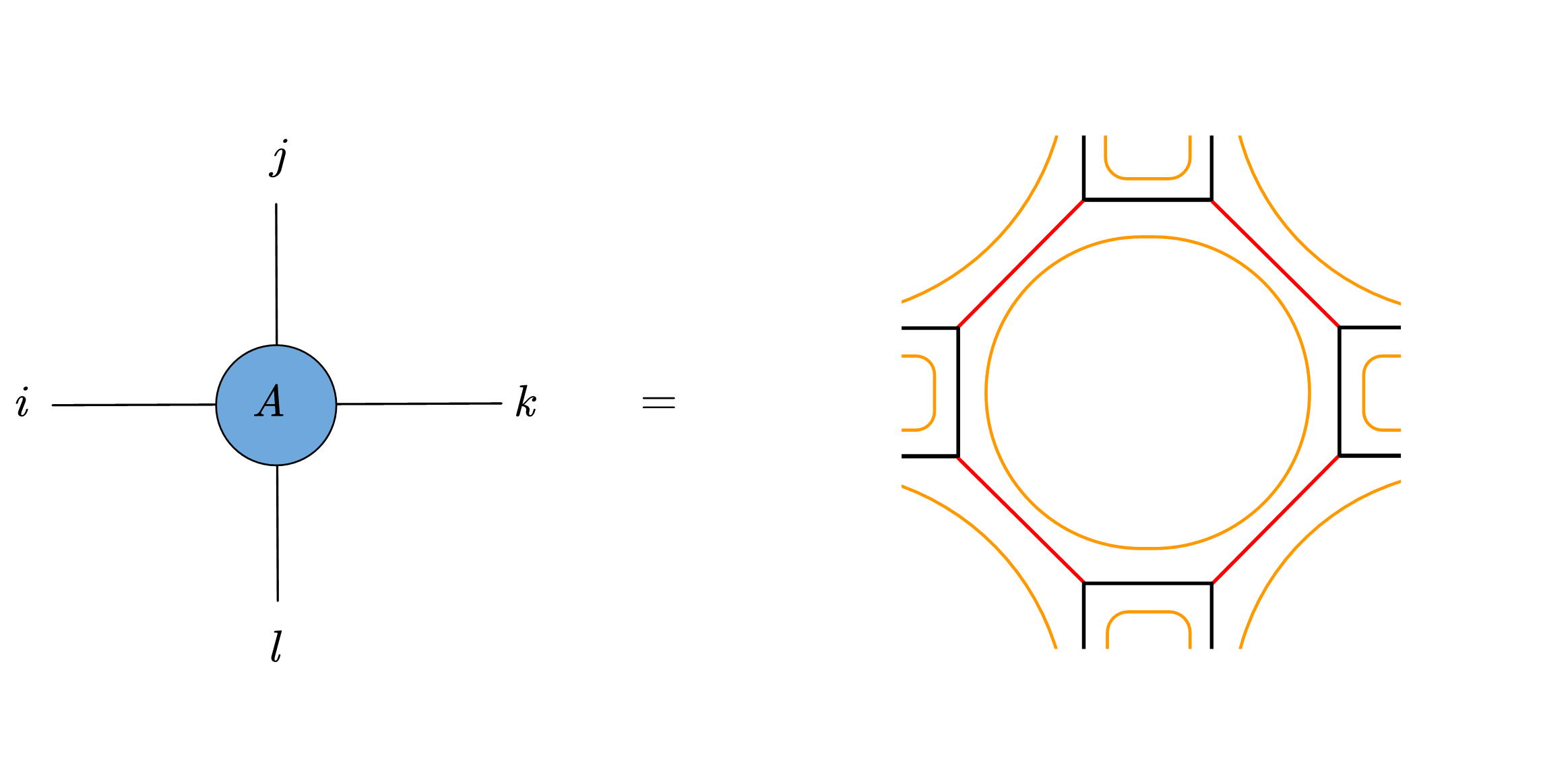
where we use to represent the contraction of a network of 6-legged -tensors, and to represent a basis state in the Levin-Wen Hilbert space with square edges and octagon edges fixed to the labels , and etc. For the square-octagon lattice, the -tensor is shown in Fig.1(b) where and are the indices of the square edge, and is the index of the octagon edge. , and are the ancillary indices necessary to decompose the possibly long-range entangled state into contraction of local tensors. In our setup of square-octagon lattice, the values of the -tensors are, up to a global constant, given by[17, 19]:
| (2) |
where is the quantum dimension of the simple object , and is the F-symbol of the input fusion category.
The fusion category has 5 simple objects, labeled by , , , and . The quantum dimensions are , , . For the fusion rules and F-symbols, we refer the readers to the appendix A.
2.2 Tensor network representation of strange correlator
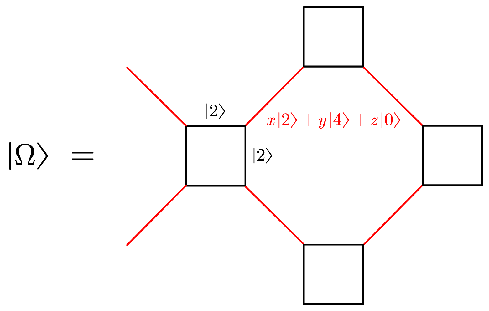
For the product state , we consider the configuration as shown in Fig.2(a). The state on each square edge is fixed to in the local Hilbert space, while the state on each octagon edge is taken to be . We impose the normalization condition ,as an overall scaling factor does not affect the system. This combination is taken to respect the fusion rule in the fusion category.
The strange correlator is obtained by taking inner product . Its tensor network representation is shown in Fig.2(b). The local tensors are contracted in this specific manner to re-express the strange correlator as a square network of tensors. In the following we may use to denote either the product state or the corresponding strange correlator when the meaning is clear from context.
3 The phase diagram
In this section we give a detailed description of the phase diagram of the strange correlator and provide numerical evidence for the identification of several critical points/lines/regions.
We continuously change the strange correlator by tuning the three parameters , and in the product state . The transfer matrix of this model is obtained by contracting a row of the tensor shown in Fig.2(b). In thermodynamic limit, the transfer matrix is represented as an infinite matrix product operator (iMPO) and its dominant eigenvector can be obtained using iMPS methods. Numerically, we use VUMPS algorithm[24] and Julia’s “MPSKit” package[26, 25] to obtain the dominant eigenvector of the transfer matrix. The entanglement entropy of the dominant eigenvector of the transfer matrix is then calculated for the half-infinite chain.
3.1 Spherical plot of entanglement entropy
This model has a two dimensional spherical parameter space under the normalization . For convenience, we also use the spherical coordinates and to describe the parameter space. The two parametrizations are related by , , . In certain cases we also use the normalization condition and projectthe phase diagram onto the plane.
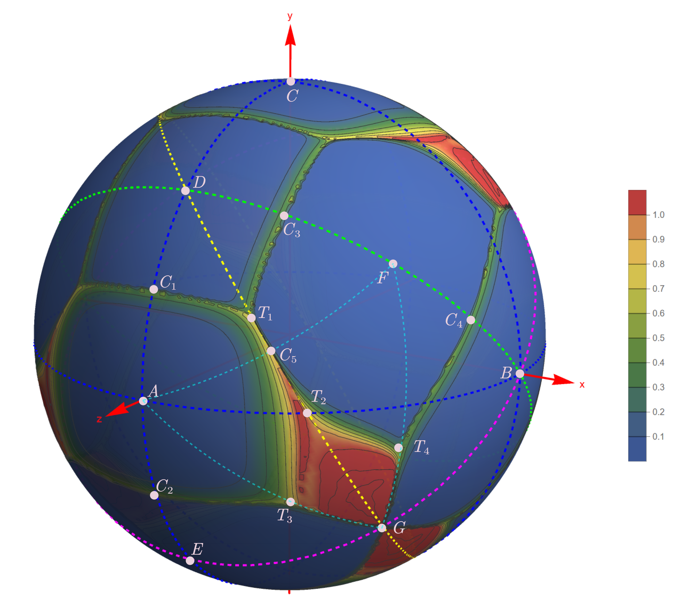
Fig.3 illustrates the phase diagram of the strange correlator as determined by the spherical contour plot of entanglement entropy. The color of the point represents the value of the entanglement entropy. The phase diagram is divided into several phases. Certain phase transition lines between gapped phases are clearly visible, indicating sharp changes in the entanglement entropy and hence in the underlying strange correlator.
-
•
Gapped phases: The gapped phases are characterized by near-zero entropy, which appear as blue regions in the plot. In Fig.3, the blue regions centered at are all gapped phases. With a slight abuse of notation, we use to denote the gapped phase centered at , where the meaning should be clear from context. The gapped phases are exactly the type I, II and III gapped phases identified in [1], which correspond to the Frobenius algebras , and respectively. The gapped phases are new gapped phases that are not identified in [1].
-
•
Gapless phases: The gapless phases are characterized by nearly maximal entropy due to long-range entanglement, and appear as red regions in the plot. The red region enclosed roughly by is a gapless phase that is not identified in [1]. We later give numerical evidence that this red region is a CFT phase with central charge .
We now give a comprehensive description of the position of various points and lines in the phase diagram.111The position of the points and can be calculated from the perspective of anyon condensation or Kramers-Wannier duality[37].
-
•
All dashed lines in Fig.3 are (part of) big circles on the unit sphere.
-
•
: These points are gapped and completely disentangled, the entanglement entropy at these points are exactly zero. are the intersection points of the axes and the unit sphere. lies at the midpoint of the arc , and lies at the midpoint of the arc . The points correspond to states , and respectively. The blue, green and magenta dashed lines are the big circles on the unit sphere that pass through these points.
-
•
: These points are critical points on the phase transition lines between gapped phases. The entanglement entropy at these points are non-zero and scale logarithmically with the effective correlation length of iMPS. The four phase transition lines on which these points lie are all of Ising type and have central charge . The critical points are located at the quadrisection points of the arcs and respectively. At these points, the phase transition lines are orthogonal to the dashed lines that interpolate neighboring gapped phases. The coordinates of these points are easily calculated from this fact. For example, under the normalization condition the points and have coordinates and respectively. The spherical coordinates of and are .
-
•
: This point is the intersection of and , and it lies at the midpoint of the arc . Its spherical coordinates are . Current numerical analysis suggests that at this point the strange correlator represents a CFT point with central charge .
-
•
: This point is the tricritical point between the three gapped phases . It is on the KW line (the yellow dashed line ) but its precise position is currently unclear. Our numerical analysis suggests the length of the arc is between and . Alternatively, under the normalization this point’s -coordinate is in the range and its -coordinate is determined by the equation of the KW line .
-
•
: This point is the intersection of the KW line and the line . The length of the arc is , and the length of arcs and are both . This point also represents a CFT.
-
•
: This line is the phase transition line between the gapped phases and . The length of the arc is . We later give numerical evidence that the central charge of this phase transition line is .
-
•
: This point is the intersection point of four phases - two gapped phases and two CFT phases. It lies at the intersection of four dashed lines: the line , the line , the line and the line . The point is the midpoint of the arc . Under the normalization this point has coordinate . Entanglement scaling at this point shows that it is not a critical point.
-
•
: These points are tricritical points between the CFT phase and two gapped phases. and are on the lines and respectively, but their precise positions are currently unknown. Later we give estimation of the -coordinate of and the -coordinate of under the normalization.
-
•
and : They are the phase transition lines between the CFT phase and the gapped phases and respectively. The central charge of these phase transition lines are . Under the normalization, the line has equation and the line has equation .
3.2 Symmetry
One of the benefits of plotting the phase diagram on the sphere is that it makes the symmetry of the phase diagram more apparent. Let denote the origin point of coordinate system. The phase diagram is symmetric under each of the following three reflections:
-
•
: This is a reflection about the plane .
-
•
: This is a reflection about the plane .
-
•
: This is a reflection about the plane .
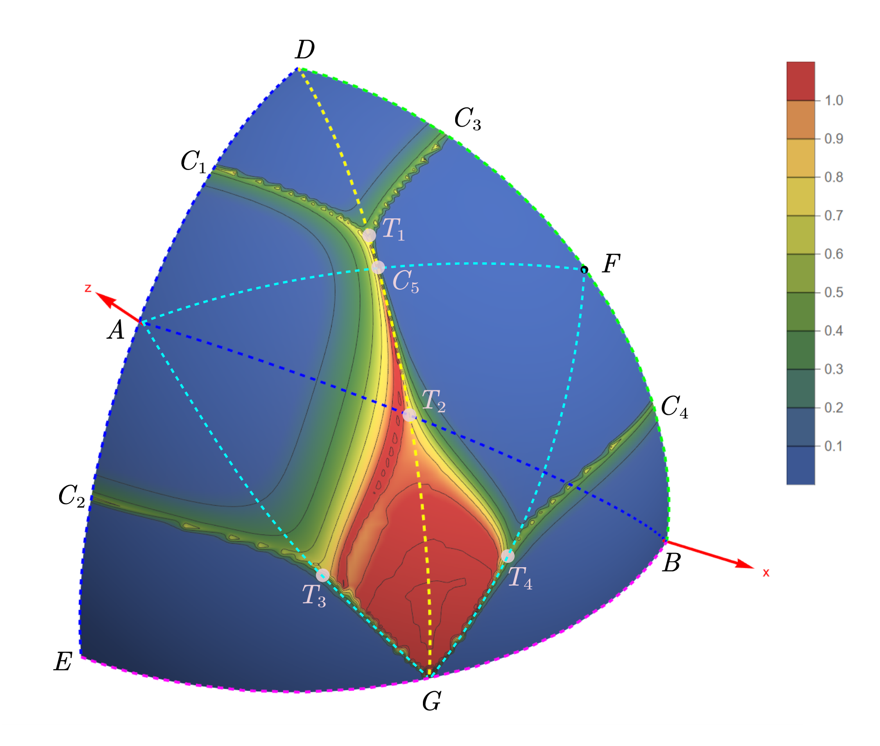
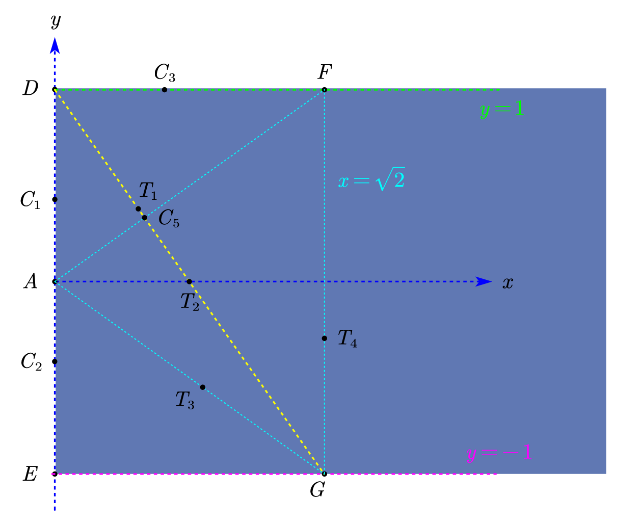
The phase diagram is symmetric under the three reflections, so the phase diagram is effectively divided into 8 equivalent regions. We take a spherical equilateral right triangle , as depicted in Fig.4(a). All other regions of the phase diagram can be obtained by applying the above reflections to this region. The spherical angles . The points are the midpoints of the arcs and respectively. The spherical triangle is also equilateral and has angles .
The symmetries are not independent. The combined application of all the three reflections brings the point to its antipodal point , which is automatically a symmetry of the system. From our construction of the tensor, the antipodal transformation leaves the tensor invariant because it contains an even number of octagon edges.
3.3 The critical points and lines
We now plot the entanglement entropy along several interesting lines on the diagram and show the entanglement scaling results of several critical points/lines. For convenience, we re-plot the region of phase diagram represented by Fig.4(a) on the plane under the normalization condition , as shown in Fig.4(b).
3.3.1 Along the line and
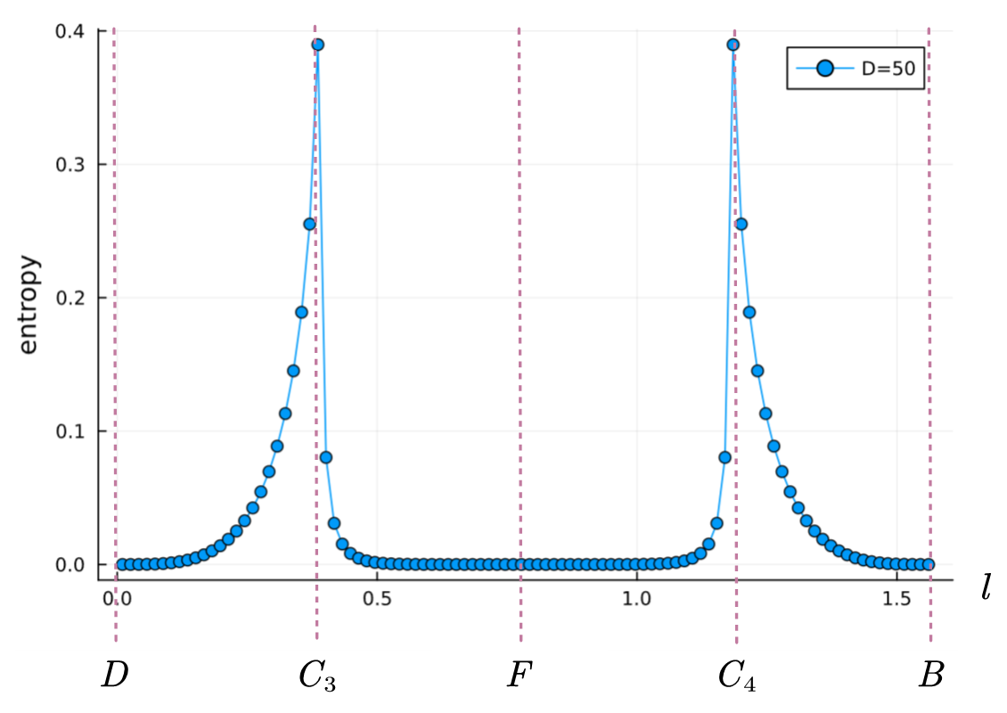
The points and are the phase transition points between neighboring gapped phases. They’re located at the quadrisection points of the arc and on the unit sphere. That’s to say all of the following arcs have length : . On the plane, the coordinates of these points are easily calculated: and have coordinates , and have coordinates . The entanglement scaling results show that all of the four critical points have central charge . In Fig.5 we show the entanglement entropy along the arc and the entanglement scaling at the point . The entropy plot has a clear peak at the point and . The entanglement entropy at and is zero because they’re the topological fixed points[1].

3.3.2 Along the KW line
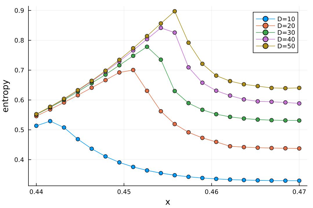
On the plane, the KW line has equation . The point and have coordinates and respectively. The entanglement scaling results suggest that both points are CFT points with central charge . The precise location of the point is currently unclear. We provide two methods to estimate the -coordinate of , and the two methods give consistent results. The first method is to plot the entanglement entropy along the line , the tricritical point should be the point where the entropy assumes a local maximum. We do this for varying iMPS bond dimension as in Fig.6, and extrapolate that the -coordinate of the peak for large bond dimension. The second method is to test entanglement scaling at the points with and respectively. The entropy- plot shows a clear linear behavior at but not at , suggesting that the system is still in the gapped phase at but has already reached the critical line at . The fit result at is . The two methods give consistent results that the -coordinate of is in the range .
3.3.3 Along the line and
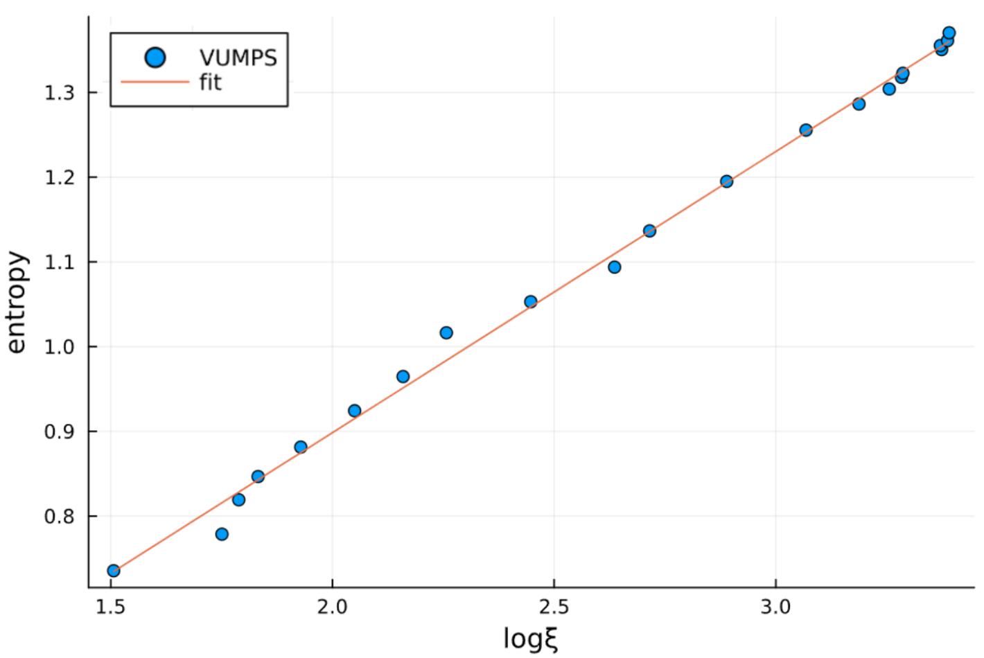
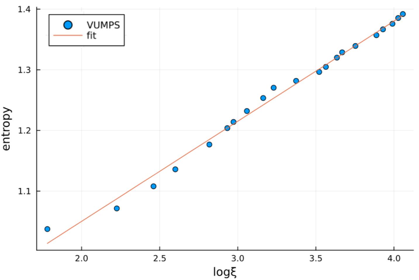
On the plane, the line has equation and the line has equation . The point and are tricritical points between the CFT phase and two neighboring gapped phases. They are located on the lines and respectively. and are critical lines. The central charge of these two phase transition lines is . The exact location of the points and remain unknown. Fig.7(a) shows the entanglement entropy along the line when the iMPS bond dimension is taken to be . The entanglement entropy grows as the system approaches . After crossing , the line is the phase transition line on which every point is a CFT point with central charge .
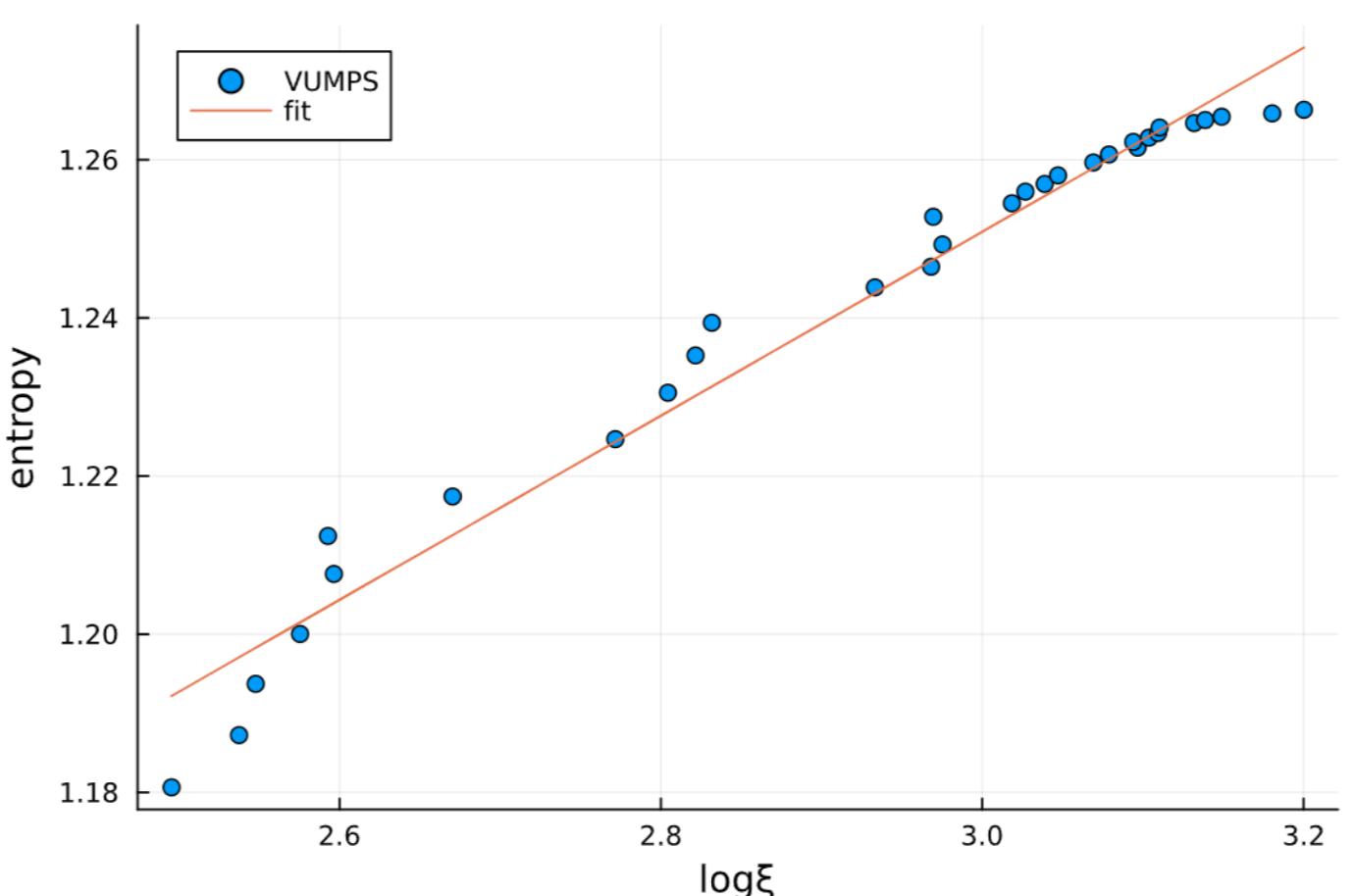
Numerical analysis shows that the -coordinate of is in the range , as can be seen from Fig.7(b) and Fig.7(c). The entropy- plot deviates from a straight line when (and ), which means the entropy tends to saturate for large bond dimension, indicating that the system is still in the gapped phase. However, when (and ), the entropy- plot shows a clear linear behavior, suggesting that the system has already reached the critical line . At this point the fit result is central charge . Using a similar strategy, we also narrow down the range of -coordinate of to be . The entanglement scaling at the point shows a central charge . We have tested many other points along the line and and all of them are consistent with central charge . Thus we conclude that the phase transition lines and both have central charge .

3.4 The CFT phase
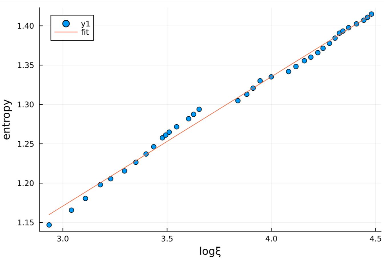
In the phase diagram Fig.3, the red region roughly enclosed by has nearly maximal entropy, indicating that it is a gapless phase. We give numerical evidence that this is indeed a CFT phase with central charge . To this end, we have tested entanglement scaling at several points in this region. And at every point we’ve seen a linear entropy- behavior, and the results are consistent with the central charge . For example, the entanglement scaling at the point and is shown in Fig.8. The first point is deliberately chosen to be close to the point which is on the phase transition line with a central charge (see Fig.7(c)). We conclude that the red region is a CFT phase with central charge .
However, in the CFT phase, only the phase boundaries and are distinctly visible and can be clearly identified in the phase diagram. The remaining phase boundaries of the CFT phase are not well resolved at the current level of numerical accuracy and require further investigation.
4 Conclusion
In this work, we have systematically investigated the interplay between topological order and criticality within the framework of the strange correlator. By employing the Levin-Wen model with an input fusion category , we constructed a tensor network representation of the strange correlator. This representation is obtained by taking the inner product with another direct product state . The state contains two tuning parameters, which allow for the interpolation between gapped topological phases and critical regimes described by CFTs.
Our numerical analysis, based on entanglement entropy computed via iMPS, yielded a detailed phase diagram on the parametric sphere.The results reveal several noteworthy features:
-
•
Phase Diagram on the Sphere: A detailed mapping of the phase diagram on unit sphere, highlighting distinct regions of gapped and critical behavior.
-
•
New Gapped and CFT Phases: Previously unidentified gapped phases were discovered, along with critical phases described by a central charge .
-
•
Phase Transition Lines with : Transitions between critical and gapped phases occur along lines characterized by a central charge of .
-
•
Explicitly Identified Critical Points: Several critical points were located precisely, with their central charge values extracted from numerical analysis.
These findings underscore the versatility of the strange correlator as a tool for bridging topological quantum field theories and critical phenomena. Future research directions include extending this framework to other fusion categories and investigating the interplay between topological phases and critical behavior. Additionally, refining numerical techniques or developing complementary analytical approaches could provide deeper insights into the mechanisms governing the transitions between topological and conformal phases in two-dimensional quantum systems.
In conclusion, our study reinforces the profound connection between topologically ordered states and conformal field theories while opening promising avenues for further exploration in quantum many-body physics.
Appendix A fusion category data
The fusion category arises from the representation theory of the affine Lie algebra and serves as an example of a fusion category. Below, we provide a concise introduction to its fundamental structures.
The fusion category consists of five simple objects, conventionally labeled as:
where is the identity object.
The quantum dimensions of the simple objects are given by , , . The fusion rules are given by
For a complete list of the F-symbols of , we refer the readers to the appendix A of [38].
Acknowledgements
We thank Ling-Yan Hung, Yidun Wan, Kaixin Ji and Yu Zhao for helpful discussions. We would also like to thank Kaixin Ji for crosschecking the F symbols in the program. We are particularly grateful to Ling-Yan Hung for a careful reading of the draft. This work is supported by the Beijing Institute of Mathematical Sciences and Applications.
References
- [1] L. Chen, K. Ji, H. Zhang, C. Shen, R. Wang, X. Zeng, and L.-Y. Hung, “Cft d from tqft d+1 via holographic tensor network, and precision discretization of cft 2,” Physical Review X 14 no. 4, (2024) 041033.
- [2] X. Chen, Z. Gu, and X. Wen, “Local unitary transformation, long-range quantum entanglement, wave function renormalization, and topological order,” Physical Review B 82 (2010) 155138.
- [3] X. Wen, “A theory of 2+1d bosonic topological orders,” National Science Review 3 (2015) 68–106.
- [4] T. Lan, L. Kong, and X.-G. Wen, “A theory of 2+1D fermionic topological orders and fermionic/bosonic topological orders with symmetries,” arXiv:1507.04673 [cond-mat] (July, 2015) . http://arxiv.org/abs/1507.04673. arXiv: 1507.04673.
- [5] H.-C. Jiang, Z. Wang, and L. Balents, “Identifying topological order by entanglement entropy,” Nature Physics 8 (2012) 902 – 905.
- [6] F. Wilczek, “Quantum mechanics of fractional-spin particles,” Physical review letters 49 no. 14, (1982) 957.
- [7] A. Y. Kitaev, “Fault tolerant quantum computation by anyons,” Annals of Physics (2003) .
- [8] A. Kitaev, “Anyons in an exactly solved model and beyond,” Annals of Physics 321 (2005) 2–111.
- [9] C. Nayak, S. Simon, A. Stern, M. Freedman, and S. Sarma, “Non-abelian anyons and topological quantum computation,” Reviews of Modern Physics 80 (2007) 1083–1159.
- [10] A. A. Belavin, A. M. Polyakov, and A. B. Zamolodchikov, “Infinite conformal symmetry in two-dimensional quantum field theory,” Nuclear Physics B 241 no. 2, (1984) 333–380.
- [11] G. Moore and N. Seiberg, “Classical and quantum conformal field theory,” Communications in Mathematical Physics 123 (1989) 177–254.
- [12] P. Francesco, P. Mathieu, and D. Sénéchal, Conformal field theory. Springer Science & Business Media, 2012.
- [13] A. Feiguin, S. Trebst, A. W. Ludwig, M. Troyer, . f. A. Kitaev, Z. Wang, and M. H. Freedman, “Interacting anyons in topological quantum liquids: The golden chain,” Physical review letters 98 no. 16, (2007) 160409.
- [14] E. Ardonne, P. Fendley, and E. Fradkin, “Topological order and conformal quantum critical points,” Annals of Physics 310 no. 2, (2004) 493–551.
- [15] D. Aasen, P. Fendley, and R. S. K. Mong, “Topological defects on the lattice: Dualities and degeneracies,” 2008.08598. http://arxiv.org/abs/2008.08598.
- [16] Y.-Z. You, Z. Bi, A. Rasmussen, K. Slagle, and C. Xu, “Wave function and strange correlator of short-range entangled states,” Physical review letters 112 no. 24, (2014) 247202.
- [17] R. Vanhove, M. Bal, D. J. Williamson, N. Bultinck, J. Haegeman, and F. Verstraete, “Mapping topological to conformal field theories through strange correlators,” Physical review letters 121 no. 17, (2018) 177203.
- [18] G. Cheng, L. Chen, Z.-C. Gu, and L.-Y. Hung, “Exact fixed-point tensor network construction for rational conformal field theory,” arXiv preprint arXiv:2311.18005 (2023) .
- [19] X. Zeng, R. Wang, C. Shen, and L.-Y. Hung, “Virasoro generators in the fibonacci model tensor network: Tackling finite-size effects,” Physical Review B 107 no. 24, (2023) 245146.
- [20] R. Wang, X. Zeng, C. Shen, and L.-Y. Hung, “Virasoro and kac-moody algebra in generic tensor network representations of two-dimensional critical lattice partition functions,” Physical Review B 106 no. 11, (2022) 115116.
- [21] O. Buerschaper, M. Aguado, and G. Vidal, “Explicit tensor network representation for the ground states of string-net models,” Physical Review B 79 (2008) 085119.
- [22] Z.-C. Gu, M. Levin, B. Swingle, and X.-G. Wen, “Tensor-product representations for string-net condensed states,” Physical Review B—Condensed Matter and Materials Physics 79 no. 8, (2009) 085118.
- [23] R. Vanhove, L. Lootens, M. Van Damme, R. Wolf, T. J. Osborne, J. Haegeman, and F. Verstraete, “Critical lattice model for a haagerup conformal field theory,” Physical review letters 128 no. 23, (2022) 231602.
- [24] V. Zauner-Stauber, L. Vanderstraeten, M. T. Fishman, F. Verstraete, and J. Haegeman, “Variational optimization algorithms for uniform matrix product states,” Physical Review B 97 no. 4, (2018) 045145.
- [25] J. Haegeman, “”tensorkit.jl julia package”,”. https://github.com/Jutho/TensorKit.jl.
- [26] M. V. Damme, “”mpskit.jl julia package”,”. https://github.com/QuantumKitHub/MPSKit.jl.
- [27] P. Calabrese and J. Cardy, “Entanglement entropy and quantum field theory,” Journal of statistical mechanics: theory and experiment 2004 no. 06, (2004) P06002.
- [28] P. Calabrese and J. Cardy, “Entanglement entropy and conformal field theory,” Journal of physics a: mathematical and theoretical 42 no. 50, (2009) 504005.
- [29] L. Tagliacozzo, T. R. de Oliveira, S. Iblisdir, and J. I. Latorre, “Scaling of entanglement support for matrix product states,” Physical Review B—Condensed Matter and Materials Physics 78 no. 2, (2008) 024410.
- [30] F. Pollmann, S. Mukerjee, A. M. Turner, and J. E. Moore, “Theory of finite-entanglement scaling at one-dimensional quantum critical points,” Physical review letters 102 no. 25, (2009) 255701.
- [31] V. Stojevic, J. Haegeman, I. McCulloch, L. Tagliacozzo, and F. Verstraete, “Conformal data from finite entanglement scaling,” Physical Review B 91 no. 3, (2015) 035120.
- [32] J. Eisert, M. Cramer, and M. B. Plenio, “Colloquium: Area laws for the entanglement entropy,” Reviews of modern physics 82 no. 1, (2010) 277–306.
- [33] F. Pollmann, C. Chamon, M. Goerbig, R. Moessner, and L. Cugliandolo, “Symmetry-protected topological phases in one-dimensional systems,” Topological Aspects of Condensed Matter Physics (Les Houches, Session CIII, 2014), Oxford University Press, Oxford (2017) 361–386.
- [34] R. Orús, “Tensor networks for complex quantum systems,” Nature Reviews Physics (2018) 1–13.
- [35] G. Evenbly and G. Vidal, “Tensor network renormalization,” Physical review letters 115 no. 18, (2015) 180405.
- [36] S. Yang, Z.-C. Gu, and X.-G. Wen, “Loop optimization for tensor network renormalization,” Physical review letters 118 no. 11, (2017) 110504.
- [37] L.-Y. Hung, K. Ji, C. Shen, Y. Wan, and Y. Zhao, “In preparation,”.
- [38] C. Levaillant, B. Bauer, M. Freedman, Z. Wang, and P. Bonderson, “Universal gates via fusion and measurement operations on anyons,” Physical Review A 92 no. 1, (2015) 012301.