The diffusive dynamics and electrochemical regulation of weak polyelectrolytes across liquid interfaces

Abstract

We propose a framework to study the spatio-temporal evolution of liquid-liquid phase separation of weak polyelectrolytes in ionic solutions. Unlike strong polyelectrolytes, which carry a fixed charge, the charge state of weak polyelectrolytes is modulated by the electrochemical environment through protonation and deprotonation processes. Leveraging numerical simulations and analysis, our work reveals how solution acidity (pH) influences the formation, interactions, and structural properties of phase-separated coacervates. We find that pH gradients can be maintained across coacervate interfaces resulting in a clear distinction in the electro-chemical properties within and outside the coacervate. By regulating the charge state of weak polyelectrolytes, pH gradients interact and modulate the electric double layer forming at coacervate interfaces eventually determining how they interact. Further linear and nonlinear analyses of stationary localised solutions reveal a rich spectrum of behaviours that significantly distinguish weak from strong polyelectrolytes. Overall, our results demonstrate the importance of charge regulation on phase-separating solutions of charge-bearing molecules and the possibility of harnessing charge-regulated mechanisms to control coacervates and shape their stability and spatial organisation.

I Introduction

In recent years, the understanding of liquid-liquid phase separation (LLPS) has gained enormous interest because of its putative role in the assembly of macromolecules (mostly proteins and nucleic acids) into membrane-less organelles (also known as biomolecular condensates) in cells [1, 2, 3]. This phenomenon has also been suggested as a primordial mechanism for compartmentalization in prebiotic cells, making it highly relevant to understanding the origin of life [4, 5, 6]. However, there are still open challenges in understanding how different molecular mechanisms affect the formation, regulation and properties of biomolecular condensates in cells due to the complex and dynamic nature of the cellular environment and its constituents [3].

Grounded in the seminal work by Flory and Huggins and experimental evidence, the balance between enthalpic and entropic interactions is considered to be the driving force of LLPS. While this is often the case, theoretical and computational studies have highlighted the important role that electrostatic interactions, mediated by the presence of ionizable groups, play in the process. By competing with entropic effects, electrostatic forces can slow down, and even arrest coarsening, potentially resulting in stable microphase separation [7, 8, 9, 10].

In physical chemistry, the process by which liquid droplets composed of charged polymers and counterions form is known as coacervation. Detailed reviews and discussions of recent advances in the experimental and theoretical studies of coacervation can be found in [11, 12]. Since the first coacervation theory proposed by Voorn and Overbeck (VO) in 1957 [13], significant efforts have been invested in extending this framework to overcome its limitations. These include field-theoretic [8, 9, 10, 14, 7, 15] and liquid-state theories, scaling arguments, and coarse-grained and (more recently) atomistic simulations that have also been vital to validate theoretical predictions. Collectively, these approaches have helped elucidate the connection between the properties of coacervates, the properties of their components and/or environmental conditions, which aided the design of smart materials– such as nano/bioreactors, drug delivery, sensors [16, 17], and understanding of cellular physiology – from the electrical excitability of cells [18, 19, 20] to the adaptive compartmentalization of the intracellular space [21, 22]. For instance, applications of random phase approximation have been used to study the impact of charges-connectivity and salt ions on the coacervation of polyelectrolyte systems [8, 14], findings that helped to explain experimental evidence about the role of intrinsically disordered domain sequences on protein LLPS  [23, 24, 25, 26].

Despite the significant advances in understanding coacervates and the role of electrostatics in liquid-liquid phase separation (LLPS), most of our understanding originates from the study of strong polyelectrolytes (i.e., polymers with approximately fixed charge). However, the majority of biomacromolecules are weak polyelectrolytes, whose charge is dynamically regulated by the local pH via protonation/deprotonation of ionizable groups. Recently, experiments have shown that coacervates of biomolecules can sustain stable pH gradients across coacervate phases, as it minimises the overall electrostatic repulsion [27] by modulating ionisation asymmetry across coacervate phases. These findings further support the putative role of biomolecular condensates in shaping pH gradients intra-cellularly and highlight the importance of charge regulation mechanisms in a theory of LLPS. There have been a few attempts at characterising the phase behaviour of weak polyelectrolytes and their pH-dependent coacervation, including experimental [28, 29], computational [30, 29] and theoretical [31, 32, 33, 34, 35, 36, 37] studies. These have revealed the complexity and interesting behaviour of weak polyelectrolyte coarcevates, which include asymmetric phase diagrams under pH-dependent conditions [33], phase separation driven by charge symmetry breaking [32] and reentrant phase behaviour arising from pH-controlled protonation equilibrium shifts [34]. Despite this progress, unexplored questions remain on how pH and electrostatics regulate the dynamics of liquid-liquid phase separation of weak, rather than strong, polyelectrolytes. This is the focus of this work.

In particular, the (diffusive) dynamics of charge-regulated macroions have only recently been addressed [38], following earlier work by the same authors on the equilibrium properties of these systems [36, 35]. In a similar spirit, in the present paper, we extend our previous work on the equilibrium properties of weak polyelectrolytes [34] to capture the dynamics and spatial arrangements of phase-separated domains near equilibrium. In our work, special emphasis is given to the role of electrostatic interactions, captured within a mean-field description, and pH gradients in the formation and properties of liquid interfaces emerging via phase separation of weak polyelectrolyte solutions. In Section II, we start by presenting the underlying statistical physics description of the charge regulation polymer solution, where we explicitly consider hydronium ions and hence have access to pH. In Section III, the dynamics of phase separation are studied both numerically and analytically, providing us with a quantitative handle on the emergence of patterns via different types of instabilities. As for strong polyelectrolytes, we find that electrostatic forces can significantly affect phase separation; in particular, we find regimes in which micro-phase separation and arrests of Ostwald ripening can occur. Interestingly, we also identify non-linear effects that, to the best of our knowledge, are unique to weak polyelectrolytes and arise from the nucleation of nano-structured bulk solutions. In Section IV, we conclude by summarising our main findings and future extension of this work; in particular, we discuss how our results highlight differences in the phase behaviour of strong and weak polyelectrolytes and possible ways forward to extend our framework to LLPS in biology.

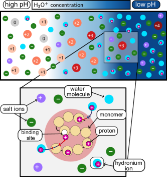
Figure 1: Schematic of the proposed model of phase-separation in ionic mixture with charge-regulated (CR) polymers. The protonation of binding sites on the polymer chains is regulated by the local pH – or, equivalently, the local concentration of hydronium ions. Upon phase separation, asymmetric distribution of charges, including hydronium (H3O+) ions, across the liquid interface results in the spatial organisation of polymer chains depending on their effective charge, here spanning from 0 to 4.

II Theoretical Model

II.1 The free energy

We consider a solution consisting of $4$ different mobile species, which we list here together with the variable for their corresponding local number density: water molecules ($c_{s}(\bm{x},t)$), positive and negative ions from a dissociated monovalent salt ($c_{\pm}(\bm{x},t)$), and weak polyelectrolytes ($c_{p}(\bm{x},t)$). We assume that H+ exists in the mixture but only bound to either water molecules or polymer monomers. Consequently, water molecules can exist in either a neutral (H2O) and protonated (H3O+) state and we denote by $\pi_{s}^{q}(\bm{x},t)$, the fraction of the water molecules in charge state $q=0,1$ at location $\bm{x}$ at time $t$. We further assume that the polyelectrolyte chains consist of $N$ monomers of which $Q_{p}$ have a group whose charge state is regulated via protonation/deprotonation, that is, absorption/desorption, respectively, of H+, resulting in $Q_{p}+1$ different charge states of the macromolecule; see Figure 1 for a schematic illustration. We denote by $\pi^{q}_{p}(\bm{x},t)$, the fraction of the macromolecules in charge state $q=0,\ldots,Q_{p}$ at location $\bm{x}$ at time $t$.

We assume that all species in the mixture are incompressible; for simplicity, we assume that solvent, counter-ions and monomers have the same molecular volume $\nu$, independently of their charge state. The molecular volume of H+ ions has indeed a negligible contribution to the molecular volume of the macromolecules and water molecules. Assuming there are no voids in the mixture, the concentration of the different species must locally satisfy

$$\nu\left(\sum_{i\in\mathcal{I}\setminus\left\{p\right\}}c_{i}(\bm{x},t)+Nc_{p}(\bm{x},t)\right)=1.$$ (1)

where the set $\mathcal{I}$ collects the subscript indicating all the species in the solution $\mathcal{I}=\left\{p,\pm,s\right\}$.

We assume that the mixture forms a dielectric medium with permittivity $\epsilon$; while this is, in general, a function of the mixture composition  [39, 26], here for simplicity, we take it to be constant. The presence of charges in the solution gives rise to an electric potential $\psi$, which satisfies the Poisson equation:

$$-\nabla\cdot\left(\epsilon\nabla\psi(\bm{x},t)\right) =e\varrho(\bm{x},t),$$ (2a)

$$\varrho(\bm{x},t) =\sum_{i\in\mathcal{I}}q_{i}(\bm{x},t)c_{i},$$ (2b)

where $e$ is the elementary charge, $\varrho$ is the local charge density of the mixture (in units of elementary charge) and $q_{i}(\bm{x},t)$ is the molecular charge of the $i$-th (in units of elementary charge). While the ions have a constant charge, $q_{\pm}\equiv\pm 1$, the charge in the solvent and on the polymer can change both spatially and temporally because of charge regulation:

$$q_{s}(\bm{x},t) =\sum\limits_{q=0}^{1}q\pi_{s}^{q}(\bm{x},t),$$

$$q_{p}(\bm{x},t) =\sum\limits_{q=0}^{Q_{p}}q\pi_{p}^{q}(\bm{x},t).$$

This contrasts with other models where the charge on macromolecules is taken to be fixed [15]. Eq. (2) relates the electric potential to the local charge density and naturally introduces a length scale $\ell_{B}=e^{2}/(4\pi\epsilon k_{B}T)$, also known as Bjerrum length, which describes the length scale at which the energy due to the Coulomb force between two charges and the thermal energy, $k_{B}T$, balance.

We assume that the mixture is maintained at constant temperature $T$ and is locally at equilibrium. Consequently, the thermodynamics of the mixture is given by the mean-field Helmholtz free energy density, $f$, which is composed of 4 terms:

$$f[c_{m},\psi]=\bar{f}(c_{m},\pi_{p}^{q})+\frac{\kappa}{2}\left|\nabla c_{p}\right|^{2}-\frac{\epsilon}{2}\left|\nabla\psi\right|^{2}+\psi e\varrho.$$ (3)

The first term, $\bar{f}$, corresponds to the bulk free-energy for a homogeneous mixture, see, e.g.,  [34, 37]:

$$\frac{\bar{f}}{k_{B}T}=c_{+}\ln\nu c_{+}+c_{-}\ln\nu c_{-}+c_{s}\sum\limits_{q=0}^{1}\pi_{s}^{q}\ln[\nu\pi_{s}^{q}c_{s}]+c_{p}\sum\limits_{q=0}^{Q_{p}}\pi_{p}^{q}\ln[N\nu\pi_{p}^{q}c_{p}]+\chi N\nu c_{p}c_{s}+c_{p}\sum\limits_{q=0}^{Q_{p}}\pi_{p}^{q}\frac{u^{q}_{\mbox{\tiny CR},p}}{k_{B}T}$$ (4)

$$+c_{s}\sum\limits_{q=0}^{1}\pi_{s}^{q}\frac{u^{q}_{\mbox{\tiny CR},s}}{k_{B}T}-\lambda_{p}\left(1-\sum_{q=0}^{Q_{p}}\pi_{p}^{q}\right)-\lambda_{s}\left(1-\sum_{q=0}^{1}\pi_{s}^{q}\right)-\lambda_{\mbox{\tiny CR}}\left(c_{H}-q_{p}c_{p}-q_{s}c_{s}\right).$$

In Eq. (4) the first 3 terms correspond to the standard Flory-Huggins contribution containing the entropy of mixing associated with each component of the mixture, the mean-field interactions between the macromolecules and water with strength $\chi$ and the internal free energies associated with different charge states $u_{\mbox{\tiny CR},m}^{q}$. We keep this expression of $q$ general in the derivation of the model, but choose a particular form later for the simulation results in Section III. For simplicity, we have assumed that $\chi$ is independent of both the macromolecule and the water charge state. In Eq. (4), $\lambda_{p}$ and $\lambda_{s}$ and $\lambda_{\mbox{\tiny CR}}$ are Lagrange multipliers associated with the normalisation condition for the charge state distributions, $\pi_{p}^{q}$ and $\pi_{s}^{q}$, and the local conservation of H+ ions by the charge regulation mechanisms. Indeed, protonation/deprotonation reactions only result in the exchange of charge between species, leading to the local number density of H+ ions

$$c_{H}(\bm{x},t)=q_{s}(\bm{x},t)c_{s}(\bm{x},t)+q_{p}(\bm{x},t)c_{p}(\bm{x},t),$$ (5)

to be conserved. The second term in Eq. (3) accounts for the energy cost associated with the phase-separated polymer-rich and polymer-poor regions, which scales with the interfacial tension $\kappa$. For simplicity, we assume the latter to be constant, i.e., independent of the mixture composition. Note that in writing Eq. (3) we have neglected the contribution due to the gradient cost associated with the salt, which has been investigated in [15]. The last two terms on the right-hand side of Eq. (3) account for the electrostatic energy of the mixture [40].

II.2 The CR-mechanisms

For simplicity, we assume that charge regulation mechanisms occur at a much faster time scale than molecule transport. As a result, the local polymer and solvent charge distribution $\left\{\pi_{p}^{q}\right\}_{q=0}^{Q_{p}}$ and $\left\{\pi_{s}^{q}\right\}_{q=0}^{1}$ can be obtained by minimising the free-energy density $\bar{f}$ (see Eq. (4)) with respect to $\pi_{p}^{q}$. This procedure is equivalent to imposing the detailed balance for the charge regulation mechanisms (see [34] for more details). Completing the minimization yields a similar result as described in [34] for the polymer and water charge distributions

$$\pi_{s}^{q} =\frac{\exp\left(-\beta(u^{q}_{\mbox{\tiny CR},s}+\tilde{\alpha}q)\right)}{\sum\limits_{\zeta=0}^{1}\exp\left(-\beta(u^{q}_{\mbox{\tiny CR},s}+\tilde{\alpha}\zeta)\right)},\quad q=0,1,$$ (6a)

$$\pi_{p}^{q} =\frac{\exp\left(-\beta(u^{q}_{\mbox{\tiny CR},p}+\tilde{\alpha}q)\right)}{\sum\limits_{\zeta=0}^{Q_{p}}\exp\left(-\beta(u^{\zeta}_{\mbox{\tiny CR},p}+\tilde{\alpha}\zeta)\right)},\quad q=0,\ldots,Q_{p},$$ (6b)

where $$\beta=(k_{B}T)^{-1}$$ and the function

$$\tilde{\alpha}=e\psi+\lambda_{\mbox{\tiny CR}}$$ (6c)

captures the contribution of the local environmental conditions in regulating protonation/deprotonation reactions. Note that the multiplier $\lambda_{\mbox{\tiny CR}}$ is implicitly defined in terms of the local number density of H+ ions by Eq. (5). This is apparent when introducing the partition function $\mathcal{Z}_{m}(\tilde{\alpha})=\sum\limits_{q=0}^{Q_{m}}\exp\left(-\beta(u^{q}_{m,\mbox{\tiny CR}}+\tilde{\alpha}q)\right)$, which contains the necessary information on the distribution $\pi_{m}^{q}$ as the $j$-th cumulant of $\pi_{m}^{q}$, $\mathcal{Q}^{(j)}_{m}$, which is given by

$$\mathcal{Q}^{(j)}_{m}=k_{B}T\frac{d^{j}}{d\tilde{\alpha}^{j}}\ln\mathcal{Z}_{m}(\tilde{\alpha})\,.$$ (7)

II.3 Diffusive dynamics

The motion of the different species in the solution yields changes to their local number densities $c_{p}$, $c_{s}$, $c_{\pm}$, but can also drive changes in the local number density of the H+ ions, $c_{H}$. The conservation of mass associated with the different species is expressed by:

$$\partial_{t}c_{m}+\nabla\cdot(c_{m}\bm{v})+\nabla\cdot\bm{j}_{m}=0,$$ (8a)

for $$m\in\mathcal{I}_{H}=\left\{p,\pm,H,s\right\} \bm{v} \bm{j}_{m} \bm{v}\equiv 0 \bm{j}_{s}+N\bm{j}_{p}+\bm{j}_{+}+\bm{j}_{-}=0 P$$. In Eq. (8a), is the mixture velocity and are the thermodynamic (or diffusive) fluxes corresponding to each component. For simplicity, we here neglect hydrodynamic effects and, subsequently, take the mixture velocity . As a result, we only have diffusion-type fluxes in (8a). Note that the fluxes are not independent, rather they must satisfy the following constraint to be consistent with the no-void condition (1). This constraint can be weakly enforced by introducing the thermodynamic pressure .

The form of the thermodynamic fluxes and pressure are derived using the Maxwell-Stefan approach (details are given in Appendix A). Under the assumption that the friction coefficients between the different components are proportional to their molecular volumes and independent of their charge states, the Maxwell-Stefan conditions are easily invertible and we obtain an explicit definition of the fluxes:

$$\bm{j}_{m}=-\sum_{K\in\mathcal{I}_{H}}\mathcal{M}_{mK}\nabla\mu^{\text{el}}_{K},\quad m\in\mathcal{I}_{H},$$ (8b)

where $\mathcal{M}_{mK}$ is the mobility matrix and the variables $\mu^{\text{el}}_{m}$ are the electro-chemical potentials for the different components of the mixture. Based on our assumption $\mathcal{M}$ is almost diagonal (see Eq. (21)) and cross-terms only arise to account for the couplings between the movement of proton-carrying molecules (i.e., solvent and polymer) and H+ ions (see Appendix A for more details).

The electrochemical potentials for the components $i\in\left\{\pm,s,p\right\}$ of the mixture have the standard form:

$$\mu^{\text{el}}_{i}=P\nu_{i}+q_{i}e\psi+\frac{\partial\bar{f}_{\mbox{\tiny eff}}}{\partial c_{i}}-\kappa_{i}\nabla^{2}c_{i},\quad i\in\mathcal{I},$$ (8c)

while we find that the chemical potential for the H+ ions is set by the Lagrange multiplier associated with the charge regulation, $\mu^{\text{el}}_{H}=-k_{B}T\lambda_{\mbox{\tiny CR}}$. In Eq. (8c), $\nu_{i}$ indicates the molecular volume of the $m$-th component ($\nu_{p}=N\nu$ and $\nu_{s,\pm}=\nu$ otherwise), $P$ is the thermodynamic pressure (see Eq. (18)), $q_{i}$ is the molecular charge associated with each component, $\bar{f}_{\mbox{\tiny eff}}$ is the effective free energy and the interfacial tension parameter $\kappa_{i}$ is non-zero only for $i=p$. The form of the effective free energy is obtained by substituting Eqs. (6b) into Eq. (4)

$$\begin{aligned} \frac{\bar{f}_{\mbox{\tiny eff}}}{k_{B}T}&=c_{s}\ln[\nu c_{s}]+c_{+}\ln\left[\nu c_{+}\right]+c_{-}\ln\left[\nu c_{-}\right]+c_{p}\ln\left[\nu Nc_{p}\right]+\chi N\nu c_{p}c_{s}-c_{H}\lambda_{\mbox{\tiny CR}}\\[2.0pt] \qquad&-c_{p}\left(\ln\left[\mathcal{Z}_{p}(\tilde{\alpha}(\psi,\lambda_{\mbox{\tiny CR}}))\right]+eq_{p}\psi\right)-c_{s}\left(\ln[\mathcal{Z}_{s}(\tilde{\alpha}(\psi,\lambda_{\mbox{\tiny CR}}))]+eq_{s}\psi\right).\end{aligned}$$ (8d)

To summarise, the system (8) governs the dynamics of the mixture composed of charged components, some of which can locally regulate their charge via the presence of ionizable groups. Electrothermodynamics forces (i.e., gradients in the chemical potentials) drive the dynamics of the system towards its thermodynamic equilibrium and are influenced by the electrostatics of the mixture via the electrostatic potential $\psi$ defined by the Poisson equation, Eq. (2), and charge regulation. The CR mechanisms enter the problem via the multiplier $\lambda_{\mbox{\tiny CR}}$ – corresponding to the electrochemical potential of H+ ions – and the moments of the charge distributions associated with the components that present ionizable groups, which are locally defined by the non-linear algebraic system given by Eqs. (5)-(6).

The non-linearities in the model prevent its analytic solution and we therefore solve the dynamic equations numerically. We consider the simplest case of an isolated system consisting of a domain $\Omega$ and impose fluxes and stresses to vanish at the boundary of the domain:

$$\bm{j}_{m}\cdot\bm{n} =0,\quad\bm{x}\in\partial\Omega,\quad m\in\mathcal{I}_{H}$$ (9a)

$$\nabla\phi_{p}\cdot\bm{n} =0,\quad\bm{x}\in\partial\Omega,$$ (9b)

$$\quad\nabla\psi\cdot\bm{n} =0,\quad\bm{x}\in\partial\Omega.$$ (9c)

The no-flux conditions imply that the total concentration of all species in the domain is conserved over time, while the condition (9c) implies that there is no net electric field across the solutions and requires the solution to be electroneutral:

$$\int_{\Omega}\varrho(\bm{x},t)d\bm{x}\equiv 0.$$

However, this condition only imposes $$\psi$$ up to a constant. We therefore need to impose an additional constrained on its value; without loss of generality we require:

$$\psi(0,t)=0.$$ (9d)

For the problem to be well-posed the initial conditions on the number densities ($c_{H}$, $c_{p}$, $c_{s}$, $c_{\pm}$) must satisfy global electroneutrality of the solution and the no-void condition, i.e., Eq. (1), locally.

III Results

We now employ the derived quantitative theory and a combination of numerical and analytical approaches to study the time-evolution and long-term behaviour of phase-separated CR polymer solutions. For simplicity, we focus on flat interfaces and consider a 1D problem defined on the interval $\Omega=\left[0,L\right]$, where $L$ is the size of the domain. We present the non-dimensional 1D form of the modelling equations in the Supplementary Material (SM). Following the literature on dilute electrolyte solutions [41], we scaled space by the Debye-like scale $L_{\psi}=\sqrt{\epsilon\nu k_{B}T}/e$, even though this deviates from the typical screening length for non-dilute weak polyelectrolytes; more details in Section III.2. Details on the numerical approach to solving the time-dependent problem and parameter values used in the simulations are given in the SM. For the numerical simulations, a specific model for the charge regulation mechanisms must be specified. Here, we use the standard linear-quadratic form for the charge regulation energy as in [34, 37].

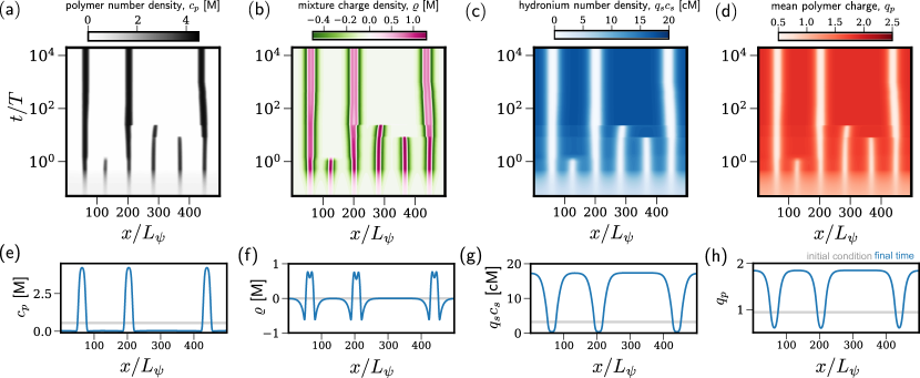
Figure 2: Charge and phase-separation dynamics predicted by the model. Top: plots illustrate the time evolution of (a) the local polymer number density $c_{p}$, in units of molar; (b) the local charge density of the mixture $\varrho$, in units of molar (defined in Eq. (2)); (c) the local number density of hydronium ions $q_{s}c_{s}$, in units of centi-molar; (d) the local mean charge on the polymer macromolecules $q_{p}$. Bottom: plots illustrate the spatial distribution at the initial ($t/T=0$) and final ($t/T=20000$) simulation times for (e) $c_{p}$, (f) $\varrho$, (g) $q_{s}c_{s}$, and (h) $q_{p}$. Model and scaling parameters are listed in the SM.

III.1 Coacervation dynamics of weak polyelectrolytes

We start by discussing the dynamics of phase separation of an initially homogeneous mixture when perturbed by introducing noise in the initial concentration of polymer macromolecules in a regime where demixing occurs. The stability of homogeneous mixtures of weak polyelectrolytes will be discussed in Section III.2.

The initial perturbations in the polymer number density rapidly lead to the formation of regions of higher liquid density (Figures 2 and 2). As in recent works [7, 10, 15, 42], we observe the separation of the charges across the condensate liquid interface which results in the local breaking of charge electroneutrality at the condensate interface. While the mixture is neutral in the dilute homogeneous regions of the domain (see Figures 2 and 2), an electric double-layer forms across the condensate interface due to the asymmetric distribution of the charges in the mixture that jumps from being slightly negative outside the condensed regions to being positive in their interior. In the initial transient, we observe standard Ostwald ripening dynamics whereby smaller condensates transfer mass towards the larger domains (see Figure 2) and eventually disappear. While the smaller condensates present at earlier times are highly positively charged, as their number decreases and size increases via coarsening, their interior tends to be less positively charged (see Figures 2 and 2). At longer times ($t\approx 100T$), we observe mass is transferred from the larger (middle) to the smaller (left) domain. This inverse transfer of material stabilises the coexistence of the three equally-sized domains that persists until the end of the simulations ($t=20000T$). The stabilisation of the microscopic domains at long times is well-understood and arises from the competition between two mechanisms [8]. On the one hand, the electrostatic forces favour the asymmetric distribution of co-ions and counter-ions across the domain interface to balance the accumulation of the charged polymer phase in the condensed region and restore electroneutrality. On the other hand, the salt ion entropy favours homogeneous salt distribution by driving diffusive fluxes across the domain interface.

An interesting aspect resulting from the inclusion of the CR mechanism is the significant redistribution of free H3O+ ions in the solution during phase separation (Figures 2 and 2), leading to spatial regulation of the local pH of the mixture. In particular, we find that H3O+ ions are excluded from the condensed domains and accumulate in the more dilute regions. This is in line with predictions of asymmetric proton partitioning in weak simple coacervates [34]. The local modulation of the mixture acidity via phase separation results in the self-organised arrangement of the polymer molecules across the liquid interphase depending on their charge state (Figures 2 and 2). In particular, we find that the more highly charged polymer chains are located in the dilute area of the domains, where H3O+ ions are most abundant, while the condensed regions are occupied by the poorly charged macromolecules.

We now study how the dynamics of phase separation are affected by the average concentration of H+ ions in solution – which is a conserved quantity over time:

$$c^{0}_{H}=\frac{1}{L}\int_{0}^{L}c_{H}(x,0)\,dx.$$

The following simulation results were generated with the same random initial condition for the polymer volume fraction to ensure an appropriate comparison between the different conditions.

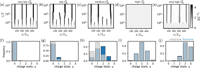
Figure 3: Simulation of the dynamics of phase separation for increasing value of the control parameter $c_{H}^{0}$. Top: plots illustrate the spatio-temporal evolution of the polymer concentration for (a) $\nu c_{H}^{0}=0.0001$; (b) $\nu c_{H}^{0}=0.001$ and (c) $\nu c_{H}^{0}=0.01$; (d) $\nu c_{H}^{0}=0.032$; (e) $\nu c_{H}^{0}=0.063$. Bottom: plots compare the spatially-average polymer charge distribution, $\bar{\pi}^{q}_{p}(t)=(\int_{0}^{L}\pi_{p}^{q}(x,t)dx)/L$ at the initial and final time of the simulations for (f) $\nu c_{H}^{0}=0.0001$; (g) $\nu c_{H}^{0}=0.001$ and (h) $\nu c_{H}^{0}=0.01$; (i) $\nu c_{H}^{0}=0.032$; (j) $\nu c_{H}^{0}=0.063$. Note that Figure 3 and Figure 2 are identical. Model parameters are as in Figure 2.

In Figure 3, we compare the coarsening dynamics (top panels) and the impact of phase separation on the overall polymer charge distribution (bottom panels) for increasing values of $c_{H}^{0}$. We find that the propensity of the mixture to phase separate depends non-monotonically on $c_{H}^{0}$. In particular, we find that while the homogeneous state is unstable at low and at very high levels of acidity, intermediate levels of acidity can favour mixing, see Figure 3. This is in line with previous analysis of the equilibrium behaviour of CR mixtures [34], which identified non-linear dependence of demixing on solution acidity as a key feature of this system. In either very low or very high $c_{H}^{0}$ values, the polymer phase exhibits minimal charge heterogeneity in the homogeneous initial state: most polymers are uncharged at very low $c_{H}^{0}$, and highly charged at very high $c_{H}^{0}$. under these limiting conditions, we find that the homogeneous states are unstable, and phase separation has a negligible impact on the overall charge distribution. Charge-heterogeneity in the initial homogeneous state peaks for intermediate $c_{H}^{0}$ values (Figures 3 and 3). Due to the convexity of the entropic term $\sum_{z}\pi_{z}\ln(\pi_{z})$ in Eq. (4), homogeneous states characterised by larger polymer charge heterogeneity are associated with higher entropy. At medium $c_{H}^{0}$ values, the homogeneous state remains unstable and we observe a significant increase in the overall charge-heterogeneity upon spatial segregation of polymers in micro-domains. In contrast, for a high value of $c_{H}^{0}$ (Figure 3) the homogeneous state stabilises to noisy initial conditions. This corresponds to the initial state of maximal charge heterogeneity suggesting that the contribution of charge heterogeneity to the entropy is sufficiently strong (at least for the parameter value considered) to compete with short-range interactions to counteract the tendency of the polymers to phase separate and stabilise the homogeneous state.

For conditions under which demixing occurs, in line with previous observations, phase separation initially follows a standard Ostwald ripening dynamics, whereby smaller condensates form and then dissipate to transfer mass towards the larger domains. The timescale at which condensed domains first appear as well as their initial number is controlled by $c_{H}^{0}$. This number decreases with $c_{H}^{0}$ in the low-medium acidity regime, then increases again upon re-entrance in the demixing region at very high acidity. It turns out that the same trend holds for the number of long-lasting condensed domains. Interestingly, for low values of $c_{H}^{0}$ – corresponding to an initially weakly charged polymer solution, we observe that condensed regions of different sizes persist. In contrast, in the medium and very high acidity case the remaining condensates have similar sizes (see Figures 3 and SM1). This suggests that medium values of $c_{H}^{0}$ stabilise the structure of long-lasting micro-domains. We validate this hypothesis further by running ensemble simulations of the model for the same environmental condition but different noisy initial conditions and characterising the micro-domains size distributions at later times – $t/T=1000$ (Figure SM1); the results are detailed in the SM. We find that $c_{H}^{0}$ modulates the level of heterogeneity in micro-domain size, with medium levels of acidity reducing variability. On the one hand, this is due to the long-term coexistence of micro-domains of distinct size in low acidity conditions (Figure 3); additionally, this reflects variability in the number of micro-domains that persist at later times. For example, for very low $c_{H}^{0}$, out of 48 simulations, we observe three or four micro-domains with approximately equal probability. In contrast, for medium $c_{H}^{0}$, the three micro-domains are highly likely; we observed them in 44 out of 48 randomly initialised simulations. These results suggest the system admits multiple spatially heterogeneous equilibria, whose stability and existence are regulated by the total proton concentration, $c_{H}^{0}$.

III.2 Emergence and coexistence of localised domains

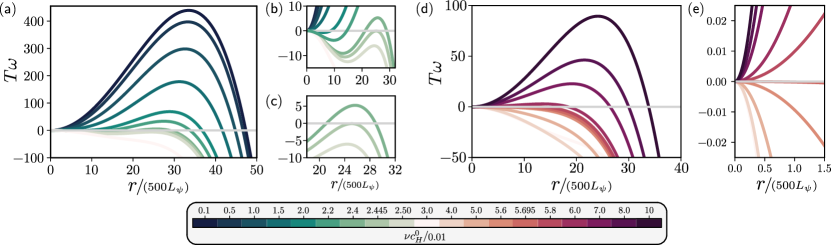
Figure 4: Dispersion relation, $\hat{\omega}_{r}=\max\left\{\omega_{r}\in\mathbb{R}\mbox{ s.t. Eq.~(\ref{eq:dispertion_relation}) holds}\right\}$, computed for for the parameter values used in Figure 3 as a function of the solution acidity (a)-(c) $\nu c_{H}^{0}\in[0.001,0.03]$ and (d)-(e) $\nu c_{H}^{0}\in[0.03,0.1]$. (b)-(c) Insets zooming into the region near the onset of low-$c_{H}^{0}$ instability from panel (a). (d) Insets zooming into the region near the onset of high-$c_{H}^{0}$ instability from (e). Model parameters are as in Figure 2.

Our previous results have shown that polymer solubility, phase separation dynamics and the length-scale selection of the long-term patterns are controlled by the total amount of H+ions; further investigation of the charge distribution hints at the role that charge-heterogeneity plays in shaping the phase behaviour of polymers under variable pH. Inspired by the presented dynamical simulations, we now focus on investigating the mechanisms driving the emergence of spatial patterns.

III.2.1 Linear stability of homogeneous weak polyelectrolytes

Firstly, we analyse the linear stability of well-mixed electroneutral solutions; details of the analysis are presented in the SM. We consider spatio-temporal perturbations of the solution of the form:

$$c_{i}=c^{0}_{i}+\delta u_{i}(\bm{x},t),\quad\psi=\delta u_{\psi}(\bm{x},t),$$ (10)

where $m\in\left\{p,\pm,s,H\right\}$ $\delta\ll 1$. We again consider the 1D problem: $\bm{x}=x\bm{e}_{x}$, $x\in[0,L]$. Substituting Eq. (10) in the original modelling equations, keeping only the linear terms in $\delta$, we obtain a linear set of coupled PDE, which we solve using standard separation of variable techniques by writing

$$u_{i}=U^{r}_{i}\cos\left(r\pi x\right)e^{\omega t},\quad i\in\left\{p,\pm,s,H,\psi\right\}.$$ (11)

where $\omega$ is the growth rate of the perturbation associated with the wavenumber $r$. In what follows, we consider a semi-infinite domain so that the wavenumber $r$ can take values on the positive real line, i.e., $r\in(0,\infty)$. This approximation, which neglects the second no flux conditions at $x=L$, is reasonable as long as the characteristic length scale of the observed pattern is significantly smaller than $L$. The growth rates $\omega_{r}$ associated with the wave number $r$ are given by the solution of a generalised eigenvalue problem,

$$\det\left[\bm{\mathsf{A}}_{r}-\bm{\mathsf{B}}\omega_{r}\right]=0.$$ (12)

The matrices $\bm{\mathsf{B}}\in\mathbb{R}^{4\times 4}$ and $\bm{\mathsf{A}}_{r}\in\mathbb{R}^{4\times 4}$ are symmetric matrices which are derived in the SM. The matrix $\bm{\mathsf{B}}$ is independent of the wavenumber $r$ and is totally positive (hence positive definite) provided $c_{j}^{0}>0$. Both $\bm{\mathsf{A}}_{r}$ and $\bm{\mathsf{B}}$ are symmetric, hence the growth rates $\omega_{r}$ are real for all wavenumbers $r$. This rules out the possibility of oscillatory instabilities. In the linear regime, the onset of patterns can therefore only result from stationary instabilities and the boundary of the stability region for homogeneous solutions can be studied by looking at the reduced problem of finding $r^{*}>0$ such that $\det\bm{\mathsf{A}}_{r^{*}}=0$.

Figure 4 illustrates how the dispersion relation changes as a function of $c_{H}^{0}$. When $c_{H}^{0}$ is either very small or sufficiently large (dark curves in either Figure 4 or Figure 4), we recover the same qualitative behaviour as for a standard conservative Cahn-Hilliard model. In this case, the growth rate $\omega$ monotonically increases with $r$ up to a local maximum, corresponding to the fastest growing spatial mode – which determines the evolution of the system in the very early stages of spinoidal decomposition, and then decreases monotonically to $-\infty$. As a result, all eigenmodes below a critical value of $r_{\rm{II}}$ have a positive growth rate $\omega$. This implies that the homogeneous state is unstable to both short- and long-wave perturbations.

As the solution acidity increases from $\nu c_{H}^{0}=0.001$ to $\nu c_{H}^{0}=0.03$, that is, from dark to light green colour curves in Figure 4, we observe a significant change in the shape of the dispersion curve which now presents two local extremal points in $r\in(0,\infty)$ (Figure 4). Despite the gradient structure of the modelling equation, the growth rate associated with small wavenumbers becomes negative, while larger wavenumbers remain unstable. As a result, the homogeneous steady state is unstable to short-scale perturbations while it remains stable to large-scale perturbations (corresponding to $r\rightarrow 0$). The damping of the large-scale instabilities is common in system coupling gradient systems with the Poisson equation [9, 41, 43]. As shown in the inset (see panel (c)), the instability transition due to dilution of $c_{H}^{0}$ below the critical value $\nu c^{0}_{H}=0.02445$ is associated with the typical length scale, $(r^{*})^{-1}\approx 20L_{\psi}$. Interestingly, we observe a different behaviour for the re-entrant instability observed for even larger solution acidity (see Figure 4-4). In this case, the dispersion relation presents at most one extremum for $r>0$. Upon increase in the solution acidity past the critical value $\nu c_{H}^{0}\approx 0.0568$, we find that the homogeneous state first becomes unstable to long-range perturbations and only subsequently to short-range perturbations. This corresponds to the standard picture of spinodal decomposition in Cahn-Hilliard models which is associated with macroscopic phase separation.

III.2.2 Microphase separation of weak polyelectrolytes

The presence of a short-scale instability and its connection with microphase separation is a characteristic feature of models of electrically controlled phase separation [7, 10, 9, 8] and it is exemplified by the canonical Ohta-Kawasaki (OK) model [44]. In particular, short-scale instabilities are controlled by the relative strength of short-range and long-range (i.e., Coulombic) interactions, which is captured by the non-dimensional parameter

$$\ell_{\kappa}=\frac{e}{k_{B}T\nu N}\sqrt{\frac{\kappa}{\epsilon}}.$$

When $\ell_{\kappa}\gg 1$, the cost associated with interfacial tension dominates over the electrostatic forces and the only driver of phase separation is the polymer hydrophobicity – captured by the Flory-Huggings term and phase separation is not sufficient to drive a breaking of electro-neutrality across the liquid interface [10]. In contrast, when $\ell_{\kappa}\lesssim 1$ short- and long-range interactions can compete; consequently, electrostatic forces can drive demixing in the presence of short-range charge fluctuations. As shown in [15], this can also result in the formation of charge layers near liquid interfaces. However, the analysis is more complicated in the case of concentrated solutions [41, 15], where composition-dependent effects come into play. For weak polyelectrolytes, the competition amongst entropy, long- and short-range interactions is further modulated by the CR mechanisms. This is apparent in the computation of the stability of homogeneous states, detailed in Appendix B. In particular, we find that the competition between short- and long-range interactions is captured by the effective parameter

$$\tilde{\ell}_{\kappa}=\ell_{\kappa}\sqrt{\frac{b}{a}},$$ (13a)

where

$$a =\chi^{2}c^{0}_{s}-\frac{(\nu^{-1}-\chi c^{0}_{s})^{2}}{\nu^{-1}-Nc_{p}^{0}}-\frac{1}{(N\nu)^{2}c_{p}^{0}},$$ (13b)

$$b =2c_{+}^{0}+2c_{H}^{0}+c_{p}^{0}\sigma_{p}^{0}-q_{p}^{0}c_{p}^{0}\left(1+\frac{q^{0}_{p}c_{p}^{0}}{\nu^{-1}-Nc^{0}_{p}}\right),$$ (13c)

and $\sigma_{p}^{0}=\langle q^{2}\rangle_{p}-q_{p}^{2}$ is the standard deviation of the charge distribution in the homogeneous steady state. Note that in defining $\tilde{\ell}_{k}$, we are assuming that the homogeneous solution is such that $a>0$, which is the most interesting case since $a<0$ corresponds to the entropy-dominated regime in which the steady state is stable. By looking at Eq. (13), we see that the CR mechanisms come into play via the coefficients $b$, as the latter depends on both the mean and standard deviation of the charge distribution. By entering positively into the factor $b$, $\sigma_{p}^{0}$ effectively increases $\ell_{\kappa}$, favouring the contribution from short-range interaction over electrostatics. In the linear problem, this appears by taking the variation of the mean polymer charge $q_{p}$ with respect to the electric field; therefore larger values of $\sigma^{0}_{p}$ imply the charge-state of the polymer phase is more sensitive to the electrostatic environment. In this regime, upon macrophase separation, the exclusion of protons from the condensed region can contribute to reducing the repulsion between polymers within the condensed domain and the need for charge separation across the interface. In contrast, increasing the mean charge on the polymer $q_{p}^{0}$ reduces $\tilde{\ell}_{\kappa}$ by increasing the strength of electrostatic interactions. In our model $q_{p}^{0}$ and $\sigma_{0}$ are not independent variables, but are rather set by the properties of the internal free energies of different polymer charge states $u^{q}_{\mbox{\tiny CR},p}$.

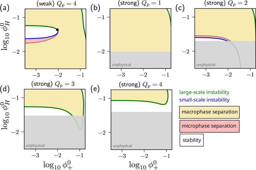
Figure 5: Spinoidal phase diagram in the $(c_{+}^{0},c_{H}^{0})$-coordinates. (a) Phase diagram for weak polyelectrolytes; same parameter values as in Figure 3. (b)-(e) Phase diagram for strong polyelectrolytes with increasing fixed charge $Q_{p}$. Black dots indicate a tricritical point (or Lifshitz point) where the microphase separation spinoidal vanishes. Microphase separation region: homogeneous state only unstable to short-range perturbations; Macrophase separation region: homogeneous state unstable to long-range perturbations; White region: homogeneous state stable to both long- and short-range perturbations. Model parameters are as in Figure 2.

We now compare the phase behaviour of weak and strong polyelectrolytes by computing the spinodal curves associated with both macro- and micro-phase separaton; or equivalently short- and long-range instabilities. In particular, we investigate the phase behaviour of weak and strong polyelectrolytes in response to the average proton concentration $c_{H}^{0}$ and the average concentration of added salt $c_{+}^{0}$. The results are shown in Figure 5, where coloured and white areas indicate phase space regions where homogeneous solutions are unstable and stable, respectively. Spinodal curves in the plot indicate codimension-one bifurcations, while the black dot indicates codimension-two bifurcations, specifically tricritical Lifshitz points, i.e., points in the phase diagram where homogeneous, micro- and macrophase separation can coexist. We find that the stability of weak and strong polyelectrolytes is controlled by both axes considered, even if in a different manner. A stabilisation of homogenous states at intermediate levels of acidity is only possible at sufficiently low salinity (the reference value used in our simulations is $\nu c_{+}^{0}=10^{-3}$).

The corresponding phase diagrams for strong polyelectrolytes are given in Figures 5 and 5 (details on the computation for the strong polyelectrolyte case can be found in the SM). Since in the weak polyelectrolyte case, molecules can exist in any charge state $q_{p}\in[1,Q_{p}]$, we compute the phase diagrams for strong polyelectrolyte with fixed charges in the same range (see Figure 5-5). Note that because of the presence of fixed charges, we have the additional constraint that $c_{H}^{0}\geq Q_{p}c_{p}^{0}$ which limits the area of the phase space which corresponds to physical states. As we increase the fixed charge $Q_{p}$ on the molecules, we find that the phase space region, in which demixing occurs, reduces. Microphase separation only occurs for medium-charged polymers with $Q_{p}=2$, while in all other cases, only macrophase instabilities are observed. When comparing the weak and strong phase diagrams, we find that the first appears like a combination of the others but also presents unique features such as the codimension-two bifurcations. This suggests the phase behaviour of weak polyelectrolytes can deviate significantly from that of strong polyelectrolytes due to the coupling between local environmental conditions and the polymer’s charge state, which allows for electro-chemical regulation of short- and long-range interactions during phase separation.

III.2.3 Analysis of localised states: the role of non-linear mechanisms.

In the previous section, we investigated the phase behaviour of weak polyelectrolytes under small amplitude perturbations, which allowed us to neglect non-linear effects. Even in the linear regime, we identify the possibility of microphase separation, i.e., the coexistence of spatially localized states. However, the evolution and interactions between such domains are eventually regulated by non-linear interactions between Coulombic and interfacial forces. Similar to the case of strong polyelectrolytes, as discussed in Section III.1, these non-linear effects influence the dynamics following macrophase separation, potentially arresting or reversing standard Ostwald ripening to stabilize the coexistence of micro-domains. Here, we discuss additional features that are unique to weak polyelectrolytes as they arise from the interaction of CR mechanisms, microphase separation and the re-entrant behaviour of the phase diagram.

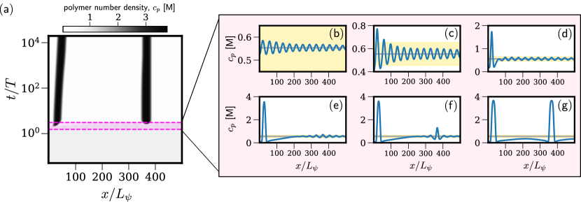
Figure 6: Simulation of the dynamics of phase separation for $\nu c_{H}^{0}=0.02425$ and $\nu c_{+}^{0}=0.001$, which lies in the region of micro-phase separation in Figure 5. (b)-(g) Plot illustrating the spatial polymer concentration at different time points within the pink-shaded area in panel (a). Note that in panels (b)-(f) the y-axis is changed. To help comparison, the grey line indicates the initial polymer concentration ($c_{p}(x,0)\approx c_{p}^{0}$) and the shaded yellow area indicates the interval $|c_{p}-c_{p}^{0}|<0.1$. Values of model parameters are as in Figure 2.

In Figure 6, we illustrate the phase separation dynamics for values of $c_{H}^{0}$ near the onset of a multiscale instability. In this regime, the linear stability analysis predicts microphase separation and selection of a persistent typical length $1/r^{*}\approx 20L_{\psi}$. We find this is what occurs in the initial transient, until $t\approx T$. Unlike in Figure 2, Ostwald ripening does not occur. On the contrary, the system quickly converges towards a layered configuration, in which small amplitude micro-domains coexist. However, after this transient, the dynamics significantly change due to a nucleation event on the left-hand side of the domain, which is driven by a small asymmetry in the initial condition (Figures 6 and 6). Interestingly, nucleation does not lead to the dissipation of the layered domains, which occupy the right-hand side of the domain (Figure 6). Eventually, a second nucleation event breaks the layered structure and drives the formation of two condensed domains that stabilise over time.

The phase separation dynamics illustrated in Figure 6 are unexpected compared to standard micro-phase separation. Although nonlinear instabilities have been reported also in models of strong polyelectrolytes, they usually preserve the layered structures and the associated length scales [41]. This indicates that the interplay between short- and long-range Coulombic interactions alone can not fully explain the observed dynamics. Instead, it suggests that this behaviour may be unique to weak polyelectrolytes and is driven by charge-regulation (CR) mechanisms.

We study the structure of localised states by looking at stationary solutions of our model, which can be obtained by setting all temporal derivatives in Eq. (8a) to zero. As detailed in the SM, the corresponding system of 5 coupled boundary value problems can be reduced to a system of two coupled boundary value problems for the stationary (rescaled) electric potential $\Psi=\Psi(x)$ and the polymer volume fraction $\Phi_{p}=\Phi_{p}(x)$:

$$-\Psi^{\prime\prime} =\tilde{F}_{\psi}(\Phi_{p},\Psi;\bm{C}_{0}),$$ (14a)

$$\ell^{2}_{\kappa}\Phi_{p}^{\prime\prime} =\tilde{F}_{\phi}(\Phi_{p},\Psi;\bm{C}_{0}),$$ (14b)

with the boundary conditions:

$$\Psi(0)=\Psi^{\prime}(\ell)=\Phi_{p}^{\prime}(0)=\Phi_{p}^{\prime}(\ell)=0,$$ (14c)

where $$\tilde{F}_{\phi} \tilde{F}_{\psi}$$, denote variations of the function

$$\begin{aligned} \tilde{F}(\phi,\psi;\bm{C}_{0})=(1-\phi)\ln\left[\gamma_{s}(\phi,\psi;\bm{C}_{0})(1-\phi)\right]\\ \qquad+\chi\phi(1-\phi)+\frac{\phi}{N}\ln\left[\gamma_{\phi}(\psi;\bm{C}_{0})\phi\right],\end{aligned}$$ (14d)

with respect to its first two scalar arguments. Because of the choice of no-flux boundary conditions, the dynamics of the number densities $$c_{m} m\in\mathcal{I}_{H} \tilde{F} \bm{C}_{0}=[c_{p}^{0},c^{0}_{+},c_{H}^{0}]$$ preserve both the local and global mass of each component . While the no-void and electroneutrality conditions constrain two of the five degrees of freedom associated with mass conservation, three additional constraints have to be specified for the computation of stationary solutions. Here we decide to impose the average number density of polymer, co-ions and protons, which emerges in Eq. (14) by the dependency of the functional on the constant vector .

Here $\Phi_{p}$ corresponds to the equilibrium polymer volume fraction so that $\Phi_{p}=1$ corresponds to the space being fully occupied by polymer molecules, while $\Phi_{p}=0$ to the space being fully occupied by the solution phase, which includes solvent, salt and hydronium ions. The system energy $\tilde{F}$ has the standard form of the energy describing the mixing of a binary mixture of non-ideal immiscible fluid phases, where the function $\gamma_{s}$ and $\gamma_{p}$ are the activity coefficients, a unitless correctional factor that describes the extent to which the component of the mixture deviates from the ideal behaviour [45].

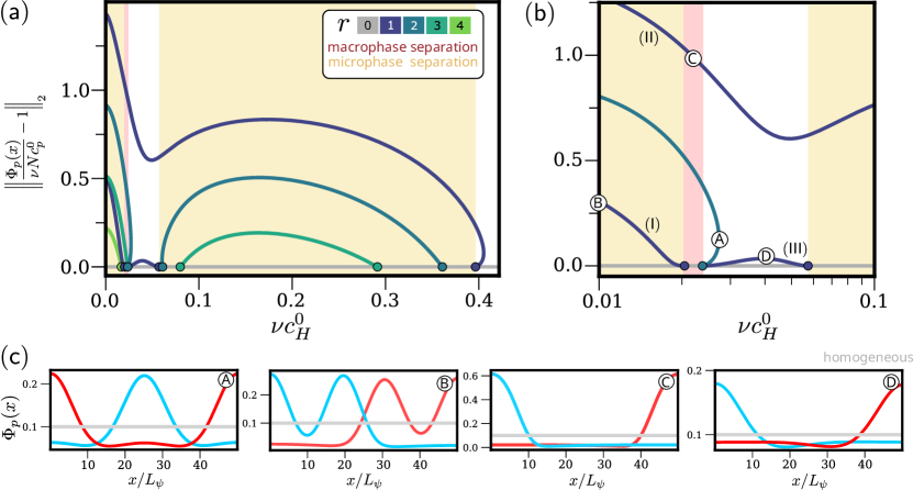
Figure 7: (a) Characteristic bifurcation diagram for Eqs. (14) using numerical continuation with $c_{H}^{0}$ as a control parameter. Here the focus is on the steady phase-separated solutions that branch from the homogeneous steady state. Shown is the normalised $L^{2}$-norm as a function of the average proton number density $c_{H}^{0}$. Different colours are used to indicate the eigenmode from which the branches first appear. Dots identify the bifurcation points of the homogeneous states, where the colour indicates the corresponding spatial modes. As in Figure 5, the yellow and red shaded area indicates the region in which the linear stability analysis predicts macro- and micro-phase separation, respectively. (b) A close-up look at the bifurcation diagram in the interval $\nu c_{0}\in[0.01,0.1]$. (c) Example profiles of the polymer spatial distribution $\Phi_{p}(x)$ corresponding to the points A-D in panel (b). Note that because of the symmetries of Eqs. (14), each branch in panels (a)-(b) corresponds to two solutions, see cyan and red curves in panel (c). Model parameters and scalings are as listed in Figure 2, except for the domain size which is reduced to $L=50L_{\psi}$.

Eqs. (14) are highly non-linear. We solve them using numerical continuation techniques which allow us to follow how solutions change as a function of a given model parameters and track local bifurcations. We unfold the structure of model solutions as a function of the control parameter $c_{H}^{0}$ (Figure 7). Since the number of solutions increases significantly with the domain size $\ell$, we consider solutions on a domain that is 10 times smaller than in the dynamical simulations ($L=50L_{\psi}$ rather than $L=500L_{\psi}$). While this simplifies the structure of the bifurcation diagram, it retains all of the interesting features that can explain the non-linear instabilities in the dynamical simulation presented in Figure 6.

While we illustrate the full bifurcation diagram for completeness (Figure 7), we focus on discussing the subpart of the diagram presented in Figure 7, that zooms in near the region of mixing for intermediate values of $c_{H}^{0}$ (Figure 7). Interestingly, we find two different types of non-linear instabilities. The first is associated with the appearance of the spatial mode $r=2$, which is characterised via a fold (or type-II) bifurcation [46] (see point A in Figures 7 and 7). Dynamical simulations reveal that of the two branches originating from (A), the one that persists at low $c_{H}^{0}$ is stable, while the one that eventually crosses the trivial solution via a subcritical pitchfork bifurcation is unstable. Similar bifurcations are observed in strong polyelectrolyte systems and can be studied analytically via weakly non-linear analysis [41, 9]. In contrast, for the eigenmode $r=1$, we find that multiple branches coexist. Branch (III), which bridges the two boundaries of the stability region, is unstable and plays an important role only in determining the critical value $c_{H}^{0}$ for re-entrant phase separation. Of the two that exist in dilute conditions (see (I) and (II) in Figure 7), branch (II) corresponds to standard macrophase separation (see point C), while branch (I) is modulated by the non-linear interactions interaction of mode $r=1$ and mode $r=3$ (see point B). Dynamical simulations reveal that branch (I) is unstable to numerical noise while (II) is stable. Eventually, branch (I) disappears by crossing the homogeneous solution; this is the point at which the linear stability analysis predicted microphase separation. However, the top branch persists beyond the end of the demixing region leading to a regime of multistability. First, a region of bistability between the micro- and macro-phase separated states (see shaded red area); then a region of tristability between the former two and the homogenous state; and finally, for even larger value of $c_{H}^{0}$, a region of bistability between the mixed and macro-phase separated solutions. This explains the possibility of nucleation of micro-phase separated states observed in Figure 6.

IV Conclusion

Building on previous studies [34, 38], we presented a theoretical framework to investigate the phase separation dynamics of weak polyelectrolytes in solutions containing protons and salt. This framework extends standard kinetic models for the coacervation of strong polyelectrolytes by incorporating charge regulation mechanisms; specifically, we account for the rapid protonation and deprotonation dynamics of binding sites along polymer chains, which regulate their charge state in response to the local solution acidity. The movement of components in the solution is guided by diffusive dynamics, via thermodynamics fluxes, and the electric field, which is accounted for via mean-field description.

We use our framework to characterize both the kinetic and equilibrium phase behaviour of weak polyelectrolytes. To do so, we integrate dynamical simulations, linear stability analysis, and numerical bifurcation analysis. These reveal the rich behaviour of weak polyelectrolytes and interesting features that distinguish their behaviour from the one of strong polyelectrolytes. Our results reveal the formation of condensed domains and the emergence of persistent pH gradients across liquid interfaces, which remain stable over long timescales (Figure 2). These sustained gradients lead to a continuous variation in the charge state of the polymer across the interface and align with experimental observations [27]. We show that the protons concentration shapes the demixing of weak polyelectrolytes in a non-linear manner, and, in the case of phase separation, it can impact the coarsening dynamics and the long-term shape and number of condensed regions. Interestingly, we observe non-standard effects– such as reverse Ostwald ripening– that lead to the stabilization of states in which multiple condensed regions coexist. This is due to the effect of long-range Coulomb forces that are driven by the asymmetric distribution of charges across the diffusive interfaces between condensed and dilute phases.

Linear stability analysis of modelling equations confirms the non-linear dependence of homogeneous solution stability on solution acidity and further reveals how acidity modulates the type of transition (or bifurcation) that leads to spontaneous demixing of weak polyelectrolytes. On the one hand, destabilisation of the homogeneous state at a high level of acidity is modulated by a large-scale instability which is typical in models of macrophase separation. In contrast, destabilisation of the homogeneous solutions at low levels of acidity is associated with small-scale (or finite size) instability, which results in stable microphase separation in which multiple condensed domains of the same characteristic size coexist stabilised by the formation of electric field driven by separation of charges across the liquid interface. While micro-phase separation can occur also in solutions of strong polyelectrolytes, our results highlight how, for weak polyelectrolytes, the existence of metastable microphase states can be controlled via modulation of the acid environment, which impact electrostatic forces via the regulation of charges on the polymer. Interestingly, full non-linear analysis of stationary solutions reveals the possibility of metastable regions in the acidity space, where the macrophase, microphase and homogeneous states are all stable introducing additional complexity that, to the best of our knowledge, has not been reported to strong polyelectrolyte systems.

This work represents an initial investigation of the complex phase behaviour of weak polyelectrolyte solutions and their ability to self-organise into localised coacervates in an environment-dependent manner. While the bifurcation analysis in Section III.2.3 reveals interesting transitions in which acidity regulates the coacervation of weak polyelectrolyte system, this study is not exhaustive and motivates further analytical and numerical exploration to fully characterize the patterns predicted by Eqs. (14). This may be achieved by leveraging the variational structure of the problem. As we show in Appendix C, Eqs. (14) can be reformulated as a 4D reversible Hamiltonian system, a class of systems known for exhibiting rich homoclinic unfolding, as exemplified in the well-known Swift–Hohenberg model for pattern formation [47]. From this point of view, generalisation of standard Maxwell construction [48] could be employed to construct such homoclinic (i.e., localised) solutions to better characterise the phase behaviour of weak polyelectrolytes in response to different control parameters (such as salt content and solution acidity). From a pattern formation perspective, it would be interesting to extend our study to non-planar interfaces to reveal the structure, interaction and regulation of weak polyelectrolyte coacervates via full 2D simulation.

The proposed theoretical framework reveals a rich and interesting range of physical behaviours that highlight the critical role of charge regulation mechanisms in shaping the formation and interactions of coacervates. However, further theoretical developments are needed to generalise our findings to liquid-liquid phase separation of biomolecules. In particular, this would require extending our framework to account for the complexity of biopolymers and of the cytoplasm. For example, we have here assumed binding sites along the polymer chain to be identical; however, biomolecules – such as protein – are often heterogeneous and consist of distinct amino acids which can differ both in their binding affinity and/or charge. From this point of view, weak polyampholytes are a better theoretical model of proteins. Our framework can easily be extended to weak polyampholytes, paving the way to a continuum theory of the dynamics of protein coacervation and how this is regulated by pH.

Appendix A Computation of the thermodynamic fluxes.

To define the fluxes we adopt the Maxwell-Stephan approach [49], which is based on balancing the friction forces between relative phases with the thermodynamic forces. An important aspect to consider in our system is the presence of heterogeneous phases that require a careful derivation of appropriate effective Maxwell-Stephan conditions. Here we assume that the friction coefficient for heterogeneous components is independent of their charge state. Then, the balance of forces acting on the $i$-th component takes the standard form:

$$\bm{\mathcal{T}}_{i}+\sum_{i\neq j}\eta_{ij}(c_{j}\bm{j}_{i}-c_{i}\bm{j}_{j})=0,\quad i,j\ \in\left\{\pm,p,s\right\}^{2},$$ (15)

where $\eta_{ij}>0$ are the friction coefficients satisfying the symmetry condition $\eta_{ij}=\eta_{ji}$, $\bm{j}_{i}$ is the thermodynamic flux for the component $i$ and $\bm{\mathcal{T}}_{i}$ is the thermodynamic force acting on the component $i$. For homogeneous components, such as salt ions, the thermodynamic force takes the standard form

$$\bm{\mathcal{T}}_{\pm}=c_{\pm}\nabla\mu^{\text{el}}_{\pm}.$$ (16)

where $\mu^{\text{el}}_{\pm}$ is the electrochemical potential (see Eq. (8c)). For heterogeneous components such as the solvent and the polymer macromolecules, the thermodynamic forces include an additional contribution associated with the presence of variable charges:

$$\bm{\mathcal{T}}_{m}=\sum_{q=0}^{Q_{m}}\bm{\mathcal{T}}^{z}_{m}=c_{m}\nabla\mu^{\text{el}}_{m}+q_{m}c_{m}\nabla\mu^{\text{el}}_{H}.$$ (17)

Summing over $i$ Eq. (15), we have the total force $\sum_{i}\mathcal{\bm{Q}}_{i}$ must vanish. This defines the value of thermodynamic pressure $P$ up to an arbitrary constant $\bar{P}$:

$$P =\bar{P}+\bar{f}_{\mbox{\tiny eff}}-\sum_{m}c_{m}\frac{\partial\bar{f}_{\mbox{\tiny eff}}}{\partial c_{m}}+\frac{\epsilon}{2}|\nabla\psi|^{2}$$ (18)

$$\qquad\qquad+\sum_{m}\kappa_{m}\left(c_{m}\nabla^{2}c_{m}-\frac{|\nabla c_{m}|^{2}}{2}\right),$$

Here we assume that the dissipation between all components scales with their molecular volume $\eta_{ij}=\eta\nu_{i}\nu_{j}\neq 0$. Then the flux of each component is simply proportional to the thermodynamic force they experience; namely:

$$\bm{j}_{m}=-\frac{\bm{\mathcal{T}}_{m}\nu}{\eta\nu_{m}}.$$ (19)

The flux of the H+ ions can be estimated by summing over the flux of H+ ions transported by both polymer and solvent macromolecules and reads:

$$\eta\bm{j}_{H} =\frac{c_{p}q_{p}}{N}\nabla\mu^{\text{el}}_{p}+c_{s}q_{s}\nabla\mu^{\text{el}}_{s}$$ (20)

$$\qquad+\left(\langle q^{2}\rangle_{s}c_{s}+\langle q^{2}\rangle_{p}\frac{c_{p}}{N}\right)\nabla\mu_{H}^{\text{el}},$$

where $\langle q^{2}\rangle_{i}$ indicates the second moment of the charge distribution associated with the component $i$; namely $\langle q^{2}\rangle_{i}=\sum_{q=0}^{Q_{i}}q^{2}\pi^{q}_{i}$. Eqs. (19)-(20) can be written in compact form given in the main text

$$\bm{j}_{m}=\sum_{K\in\left\{p,s,H,+,-\right\}}\mathcal{M}_{mK}\nabla\mu_{K}$$

by defining the mobility matrix $\mathcal{M}$ as

$$\mathcal{M}=D\beta\begin{bmatrix}\dfrac{c_{p}}{N}&0&\dfrac{q_{p}c_{p}}{N}&0&0\\[4.0pt] 0&c_{s}&q_{s}c_{s}&0&0\\[2.0pt] \dfrac{q_{p}c_{p}}{N}&q_{s}c_{s}&\langle q^{2}\rangle_{s}c_{s}+\dfrac{\langle q^{2}\rangle_{p}c_{p}}{N}&0&0\\[4.0pt] 0&0&0&c_{+}&0\\[2.0pt] 0&0&0&0&c_{-}\\ \end{bmatrix}$$ (21)

based on the following order for the indices: $p$, $s$, $H$, $+$ and $-$. In writing Eq. (21), $\beta=(k_{B}T)^{-1}$ is a constant and $D$ is the diffusion coefficient, which is related to the friction coefficient $\eta$ in Eqs. (19)-(20) via $D=k_{B}T/\eta$.

Appendix B Stability analysis

The analytical steps used in deriving the conditions for the linear stability of homogenous, electroneutral, weak polyelectrolyte mixtures are detailed in the SM. We note that in the derivation we use the non-dimensional form of the modelling equations (see SM).

Ultimately, the stability of homogeneous and electroneutral states

$$\begin{pmatrix}c_{p}\\ c_{s}\\ c_{+}\\ c_{-}\\ c_{H}\\ \psi\end{pmatrix}=\begin{pmatrix}c_{p}^{0}\\ 1-c_{p}^{0}-2c_{+}^{0}-c_{H}^{0}\\ c^{0}_{+}+c^{0}_{H}\\ c_{H}^{0}\\ 0\end{pmatrix}$$

is connected to the existence and number of real roots of the following fourth-order polynomial:

$$\ell^{2}_{\kappa}(\pi r)^{4}-2\left[\frac{\ell^{2}_{\kappa}\tilde{F}_{\psi\psi}^{0}-\tilde{F}^{0}_{\phi\phi}}{2}\right](\pi r)^{2}-\text{det}(\mathcal{H}^{0}_{\tilde{F}})=0,$$ (22)

where $\text{det}(\mathcal{H}^{0}_{\tilde{F}})=\tilde{F}^{0}_{\psi\psi}\tilde{F}^{0}_{\phi\phi}-(\tilde{F}^{0}_{\psi\phi})^{2}$ is the determinant of the Hessian of the functional $\tilde{F}$ (see Eq. (14d)) evaluated at the equilibrium point $(\phi,\psi;\bm{C}_{0})=(\nu Nc_{p}^{0},0;[\nu Nc_{p}^{0},c_{+}^{0},c_{H}^{0}])$

$$F_{\psi\psi} =q_{p}^{0}c_{p}^{0}\nu\left(1+\frac{\nu q^{0}_{p}c_{p}^{0}}{1-N\nu c^{0}_{p}}\right)-2\nu c_{+}^{0}-2\nu c_{H}^{0}-\nu c_{p}^{0}\sigma_{p}^{0},$$ (23a)

$$F_{\phi\phi} =\frac{(1-\chi\nu c^{0}_{s})^{2}}{1-\nu Nc_{p}^{0}}+\frac{\nu}{(N\nu)^{2}c_{p}^{0}}-\chi^{2}\nu c^{0}_{s},$$ (23b)

$$F_{\psi\phi} =\frac{q^{0}_{p}}{N}\frac{1-\chi\nu^{2}Nc_{p}^{0}c_{s}^{0}}{1-N\nu c_{p}^{0}}-\chi\nu(c_{H}-q_{p}c_{p}^{0}).$$ (23c)

If we denote by

$$\Delta=\left(\frac{\ell^{2}_{\kappa}\tilde{F}_{\psi\psi}^{0}-\tilde{F}^{0}_{\phi\phi}}{2}\right)^{2}+\ell_{\kappa}^{2}\text{det}(\mathcal{H}_{\tilde{F}}),$$

then we distinguish three regimes:

• When $\det\mathcal{H}_{\tilde{F}}^{0}>0$, Eq. (22) has two real roots $\left\{\pm r_{\mbox{\tiny CH}}\right\}$,

  $$r_{\mbox{\tiny CH}}=\frac{1}{\pi\ell_{\kappa}}\sqrt{\left(\frac{\ell^{2}_{\kappa}\tilde{F}_{\psi\psi}^{0}-\tilde{F}^{0}_{\phi\phi}}{2}\right)+\sqrt{\Delta}},$$

  the homogenous solution is unstable in time to spatial perturbations with modes in the interval $r\in(0,r_{\text{CH}})$.

• When $\det\mathcal{H}_{\tilde{F}}^{0}<0$, $\Delta>0$ and $\ell^{2}_{\kappa}\tilde{F}_{\psi\psi}^{0}-\tilde{F}^{0}_{\phi\phi}>0$, Eq. (22) has four real roots $\left\{\pm r^{+}_{T},\pm r^{-}_{T}\right\}$

  $$r^{\pm}_{T}=\frac{1}{\pi\ell_{\kappa}}\sqrt{\left(\frac{\ell^{2}_{\kappa}\tilde{F}_{\psi\psi}^{0}-\tilde{F}^{0}_{\phi\phi}}{2}\right)\pm\sqrt{\Delta}},$$

  the homogenous solution $\left\{\phi_{m}^{0}\right\}$ is unstable in time to spatial perturbations with modes in the interval $r\in(r_{T}^{-},r^{+}_{T})$.

• Otherwise, Eq. (22) has no real roots, the homogenous solution is linearly stable in time to spatial perturbations.

While regimes (I) and (III) are common to models of phase separation (such as classical Cahn-Holliard models), the regime (II), where the homogeneous state is unstable to small-scale but not long-scale perturbations, is associated with microphase separation. We note that the condition $\ell^{2}_{\kappa}\tilde{F}_{\psi\psi}^{0}-\tilde{F}^{0}_{\phi\phi}>0$ necessary to be in regime (II) can be expressed in terms of the characteristic length scale $\tilde{\ell}_{\kappa}=\ell_{\kappa}\sqrt{F_{\psi\psi}/F_{\phi\phi}}$ and the coefficient $a=-F_{\phi\phi}$ defined by Eq. (13) as

$$a(1-\tilde{\ell}^{2}_{\kappa})>0.$$

Taking $a>0$, this highlights how the length scale $\tilde{\ell}_{\kappa}$ mediates the transition to the regime in which microphase separation is possible.

Spinodal curves.

Spinodal curves are identified as the curves that determine the onset of the stability of the homogeneous solution. This corresponds to transitions from the regime (III) described above to either regime (I) or (II). While the former corresponds to a standard Cahn-Hilliard (or large-scale) instability the second case leads to a Turing-like (or short-scale) instability [50]. In light of this, the boundary of the Cahn-Hilliard and Turing spinodals are defined respectively by the conditions

$$\begin{cases}\text{det}(\mathcal{H}_{\tilde{F}})=0,\\ \ell_{\kappa}^{2}\tilde{F}_{\psi\psi}^{0}<\tilde{F}_{\phi\phi}^{0},\end{cases}$$ (24)

and

$$\begin{cases}\left(\ell_{\kappa}^{2}\tilde{F}^{0}_{\psi\psi}-\tilde{F}^{0}_{\phi\phi}\right)^{2}+4\ell_{\kappa}^{2}\text{det}(\mathcal{H}_{\tilde{F}})=0,\\[10.0pt] \ell_{\kappa}^{2}\tilde{F}_{\psi\psi}^{0}>\tilde{F}_{\phi\phi}^{0}.\end{cases}$$ (25)

We can further characterise the critical spatial mode $r_{T}^{*}$ selected at the onset of the Turing bifurcation, by substituting condition (25) into the definition of $r_{T}$ given above:

$$r^{*}_{T}=\frac{1}{\pi\ell_{\kappa}}\sqrt{\frac{\ell_{\kappa}^{2}\tilde{F}_{\psi\psi}^{0}-\tilde{F}_{\phi\phi}^{0}}{2}}.$$ (26)

Note that $r^{*}_{T}$ can also be expressed in terms of the characteristic length scale $\tilde{\ell}_{\kappa}$ introduced in Section III.2

$$r_{T}^{*}=\frac{1}{\pi\ell_{\kappa}}\sqrt{a\frac{1-\tilde{\ell}_{\kappa}}{2}},$$

where $a$ is as defined in Eq. (13).

A similar result holds for the case of strong polyelectrolyte solutions. Assuming that the polymer is characterised by fixed charges $Q$, then the spinoidals are still defined by the conditions given above provided that $q_{p}^{0}\rightarrow Q$ and $\sigma_{p}^{0}\rightarrow 0$ in Eqs. (23); furthermore, the possible homogeneous states are now constrained by electroneutrality which requires $\nu c_{H}^{0}\in[Q\nu c_{p}^{0},1)$.

Appendix C Spatial Dynamics.

Following the steps detailed in the SM, we reduce the problem of computing stationary solutions of the model presented in Section II to a system of two coupled, non-linear, boundary value problems (14). Here we show how Eqs. (14) can be rewritten as a 4D reversible Hamiltonian system so that localised solutions can be described as homoclinic orbits of such a system [47] in terms of the stationary (rescaled) electric potential $\Psi=\Psi(x)$ and the order parameter $\Phi=\Phi(x)$. To do so, we introduce the moments variables, $q_{\psi}$ and $q_{\phi}$ and rewrite Eq. (14) as:

$$\begin{cases}\ell^{2}_{\psi}\Psi^{\prime}&=-q_{\psi},\\ \ell^{2}_{\kappa}\Phi^{\prime}&=q_{\phi},\\ q^{\prime}_{\psi}&=\tilde{F}_{\psi}(\Phi,\Psi;\bm{\theta}),\\ q^{\prime}_{\phi}&=\tilde{F}_{\phi}(\Phi,\Psi;\bm{\theta}),\end{cases}$$ (27a)

where the prime is used to denote the spatial derivative and $\tilde{F}_{\phi}$, $\tilde{F}_{\psi}$ are the partial derivatives of a functional $\tilde{F}$ defined by Eq. (14d). As mentioned in the main text, it corresponds to the free energy of two immiscible non-ideal fluids, where the non-ideal nature is described by the activity coefficients:

$$\gamma_{s}(\phi,\psi;\bm{C_{0}}) =\frac{1}{1+e^{-\psi+\mu^{\Delta}_{+}(\bm{C}_{0})+\chi\phi}+e^{-\psi+\mu^{\Delta}_{H}(\bm{C}_{0})}+e^{\psi+\mu^{\Delta}_{-}(\bm{C}_{0})+\chi\phi}},$$ (28a)

$$\gamma_{p}(\psi) =e^{N\mu^{\Delta}_{p}(\bm{C}_{0})}\left(\sum_{q=0}^{Q_{p}}e^{-\beta u_{\mbox{\tiny CR}}^{q}-q(\psi-\mu^{\Delta}_{H}(\bm{C}_{0}))}\right)^{-1}.$$ (28b)

where $\mu_{\pm,p}^{\Delta}$ indicate the equilibrium chemical potential difference between salt and solvent, and polymer and solvent, while $\mu^{\Delta}_{H}$ is the equilibrium chemical potential of protons (both expressed in non-dimensional units). The Hamiltonian

$$\mathcal{H}=-\frac{1}{2}\left(\frac{q_{\psi}}{\ell_{\psi}}\right)^{2}+\frac{1}{2}\left(\frac{q_{\phi}}{\ell_{\kappa}}\right)^{2}-\tilde{F}(\Phi,\Psi;\bm{\theta})$$

generates Eqs. (27) and it is a first integral along trajectories in the $(\Psi,\Phi,q_{\psi},q_{\phi})$ space.

A similar formulation holds for the case of a polymer with fixed charge $Q_{p}$, except for the form of the $\gamma_{p}$ term which reduces to $\gamma_{p}(\psi)=\exp\left[Q_{p}\psi\right]$ and can take both values above and below one.

References

- Hyman et al. [2014] A. A. Hyman, C. A. Weber, and F. Jülicher, Liquid-Liquid Phase Separation in Biology, Annual Review of Cell and Developmental Biology 30, 39 (2014).
- Riback et al. [2020] J. A. Riback, L. Zhu, M. C. Ferrolino, M. Tolbert, D. M. Mitrea, D. W. Sanders, M.-T. Wei, R. W. Kriwacki, and C. P. Brangwynne, Composition-dependent thermodynamics of intracellular phase separation, Nature 581, 1476 (2020).
- Villegas et al. [2022] J. Villegas, M. Heidenreich, and E. D. Levy, Molecular and environmental determinants of biomolecular condensate formation, Nature Chemical Biology 18, 1319 (2022).
- Oparin [1965] A. Oparin, The Origin of Life, Dover books on biology and medicine (Dover, 1965).
- Bartolucci, Giacomo and Calaça Serrão, Adriana and Schwintek, Philipp and Kühnlein, Alexandra and Rana, Yash and Janto, Philipp and Hofer, Dorothea and Mast, Christof B. and Braun, Dieter and Weber, Christoph A. [2023] Bartolucci, Giacomo and Calaça Serrão, Adriana and Schwintek, Philipp and Kühnlein, Alexandra and Rana, Yash and Janto, Philipp and Hofer, Dorothea and Mast, Christof B. and Braun, Dieter and Weber, Christoph A., Sequence self-selection by cyclic phase separation, Proceedings of the National Academy of Sciences 120, e2218876120 (2023).
- Fox [1976] S. W. Fox, The evolutionary significance of phase-separated microsystems, Origins of life 7, 49 (1976).
- G. L. Celora, M. G. Hennessy, A. Münch, B. Wagner, S. L. Waters [2022] G. L. Celora, M. G. Hennessy, A. Münch, B. Wagner, S. L. Waters, A kinetic model of a polyelectrolyte gel undergoing phase separation, Journal of the Mechanics and Physics of Solids 160, 104771 (2022).
- Grzetic et al. [2021] D. J. Grzetic, K. T. Delaney, and G. H. Fredrickson, Electrostatic Manipulation of Phase Behavior in Immiscible Charged Polymer Blends, Macromolecules 54, 2604 (2021).
- Gavish et al. [2017] N. Gavish, I. Versano, and A. Yochelis, Spatially localized self-assembly driven by electrically charged phase separation, SIAM Journal on Applied Dynamical Systems 16, 1946 (2017).
- Hennessy et al. [2024] M. G. Hennessy, G. L. Celora, S. L. Waters, A. Münch, and B. Wagner, Breakdown of electroneutrality in polyelectrolyte gels, European Journal of Applied Mathematics 35, 359 (2024).
- Muthukumar [2017] M. Muthukumar, 50th Anniversary Perspective: A Perspective on Polyelectrolyte Solutions, Macromolecules 50, 9528 (2017).
- Sing and Perry [2020] C. E. Sing and S. L. Perry, Recent progress in the science of complex coacervation, Soft Matter 16, 2885 (2020).
- Overbeek and Voorn [1957] J. T. G. Overbeek and M. J. Voorn, Phase separation in polyelectrolyte solutions. theory of complex coacervation, Journal of Cellular and Comparative Physiology 49, 7 (1957).
- Rumyantsev et al. [2018] A. M. Rumyantsev, E. Y. Kramarenko, and O. V. Borisov, Microphase Separation in Complex Coacervate Due to Incompatibility between Polyanion and Polycation, Macromolecules 51, 6587 (2018).
- Majee et al. [2024] A. Majee, C. A. Weber, and F. Jülicher, Charge separation at liquid interfaces, Phys. Rev. Res. 6, 033138 (2024).
- Calvert [2009] P. Calvert, Hydrogels for Soft Machines, Advanced Materials 21, 743 (2009).
- Li [2009] H. Li, Smart Hydrogel Modelling (Springer, Berlin, Heidelberg, 2009).
- Kolan et al. [2025] D. Kolan, S. Kozawa, D. Weitzer, G. Wnek, and M. Mussel, Propagation of a Chemo-Mechanical Phase Boundary in Polyacrylate Gels, Polymer , 128039 (2025).
- Wnek et al. [2022] G. E. Wnek, A. C. S. Costa, and S. K. Kozawa, Bio-Mimicking, Electrical Excitability Phenomena Associated With Synthetic Macromolecular Systems: A Brief Review With Connections to the Cytoskeleton and Membraneless Organelles, Frontiers in Molecular Neuroscience 15, 10.3389/fnmol.2022.830892 (2022).
- Tasaki [2002] I. Tasaki, Spread of Discrete Structural Changes in Synthetic Polyanionic Gel: A Model of Propagation of a Nerve Impulse, Journal of Theoretical Biology 218, 497 (2002).
- Feng et al. [2019] Z. Feng, X. Chen, X. Wu, and M. Zhang, Formation of biological condensates via phase separation: Characteristics, analytical methods, and physiological implications, Journal of Biological Chemistry 294, 14823 (2019).
- Berry et al. [2018] J. Berry, C. P. Brangwynne, and M. Haataja, Physical principles of intracellular organization via active and passive phase transitions, Reports on Progress in Physics 81, 046601 (2018).
- Nott et al. [2015] T. J. Nott, E. Petsalaki, P. Farber, D. Jervis, E. Fussner, A. Plochowietz, T. D. Craggs, D. P. Bazett-Jones, T. Pawson, J. D. Forman-Kay, et al., Phase transition of a disordered nuage protein generates environmentally responsive membraneless organelles, Molecular cell 57, 936 (2015).
- An et al. [2024] Y. An, T. Gao, T. Wang, D. Zhang, and B. Bharti, Effects of charge asymmetry on the liquid–liquid phase separation of polyampholytes and their condensate properties, Soft Matter 20, 6150 (2024).
- Lin et al. [2016] Y.-H. Lin, J. D. Forman-Kay, and H. S. Chan, Sequence-specific polyampholyte phase separation in membraneless organelles, Phys. Rev. Lett. 117, 178101 (2016).
- Meca et al. [2023] E. Meca, A. W. Fritsch, J. M. Iglesias-Artola, S. Reber, and B. Wagner, Predicting disordered regions driving phase separation of proteins under variable salt concentration, Frontiers in Physics 11, 10.3389/fphy.2023.1213304 (2023).
- Ausserwöger et al. [2024] H. Ausserwöger, R. Scrutton, T. Sneideris, C. M. Fischer, D. Qian, E. d. Csilléry, K. L. Saar, A. Z. Białek, M. Oeller, G. Krainer, T. M. Franzmann, S. Wittmann, J. M. Iglesias-Artola, G. Invernizzi, A. A. Hyman, S. Alberti, N. Lorenzen, and T. P. J. Knowles, Biomolecular condensates sustain pH gradients at equilibrium driven by charge neutralisation (2024).
- Chollakup et al. [2010] R. Chollakup, W. Smitthipong, C. Eisenbach, and M. Tirrell, Phase Behavior and Coacervation of Aqueous Poly(acrylic acid)-Poly(allylamine) Solutions, Macromolecules 43, 2518 (2010).
- Staňo et al. [2024] R. Staňo, J. J. van Lente, S. Lindhoud, and P. Košovan, Sequestration of small ions and weak acids and bases by a polyelectrolyte complex studied by simulation and experiment, Macromolecules 57, 1383 (2024).
- Meneses-Juárez et al. [2019] E. Meneses-Juárez, C. Márquez-Beltrán, and M. González-Melchor, Influence of on the formation of a polyelectrolyte complex by dissipative particle dynamics simulation: From an extended to a compact shape, Phys. Rev. E 100, 012505 (2019).
- Adame-Arana et al. [2020] O. Adame-Arana, C. A. Weber, V. Zaburdaev, J. Prost, and F. Jülicher, Liquid Phase Separation Controlled by pH, Biophysical Journal 119, 1590 (2020).
- Majee et al. [2020] A. Majee, M. Bier, R. Blossey, and R. Podgornik, Charge symmetry broken complex coacervation, Phys. Rev. Res. 2, 043417 (2020).
- Knoerdel et al. [2021] A. R. Knoerdel, W. C. B. McTigue, and C. Sing, Transfer matrix model of ph effects in polymeric complex coacervation, The Journal of Physical Chemistry B 125, 8965 (2021).
- Celora et al. [2023] G. L. Celora, R. Blossey, A. Münch, and B. Wagner, Counterion-controlled phase equilibria in a charge-regulated polymer solution, The Journal of Chemical Physics 159, 184902 (2023).
- Zheng et al. [2021] B. Zheng, Y. Avni, D. Andelman, and R. Podgornik, Phase separation of polyelectrolytes: The effect of charge regulation, The Journal of Physical Chemistry B 125, 7863 (2021).
- Avni et al. [2019] Y. Avni, D. Andelman, and R. Podgornik, Charge regulation with fixed and mobile charged macromolecules, Current Opinion in Electrochemistry 13, 70 (2019).
- Avni et al. [2020] Y. Avni, R. Podgornik, and D. Andelman, Critical behavior of charge-regulated macro-ions, The Journal of Chemical Physics 153, 024901 (2020).
- Zheng et al. [2024] B. Zheng, S. Komura, D. Andelman, and R. Podgornik, Diffusive dynamics of charge regulated macro-ion solutions (2024), arXiv:2411.09448 .
- Liese et al. [2022] S. Liese, A. Schlaich, and R. R. Netz, Dielectric constant of aqueous solutions of proteins and organic polymers from molecular dynamics simulations, The Journal of Chemical Physics 156, 224902 (2022).
- Markovich et al. [2021] T. Markovich, D. Andelman, and R. Podgornik, Charged membranes: Poisson–boltzmann theory, the DLVO paradigm, and beyond, in Handbook of Lipid Membranes (CRC Press, 2021).
- Bier et al. [2017] S. Bier, N. Gavish, H. Uecker, and A. Yochelis, From bulk self-assembly to electrical diffuse layer in a continuum approach for ionic liquids: The impact of anion and cation size asymmetry, Phys. Rev. E 95, 060201 (2017).
- Luo et al. [2024] C. Luo, N. Hess, D. Aierken, Y. Qiang, J. A. Joseph, and D. Zwicker, Condensate size control by charge asymmetry (2024), arXiv:2409.15599 .
- Gavish and Yochelis [2016] N. Gavish and A. Yochelis, Theory of Phase Separation and Polarization for Pure Ionic Liquids, The Journal of Physical Chemistry Letters 7, 1121 (2016).
- Shiwa [1997] Y. Shiwa, The amplitude and phase-diffusion equations for lamellar patterns in block copolymers, Physics Letters A 228, 279 (1997).
- Lewis [1907] G. N. Lewis, Outlines of a New System of Thermodynamic Chemistry, Proceedings of the American Academy of Arts and Sciences 43, 259 (1907).
- Pismen [2023] L. M. Pismen, Patterns and Interfaces in Dissipative Dynamics, 2nd ed., Springer Series in Synergetics (Springer Cham, 2023).
- Champneys [1998] A. R. Champneys, Homoclinic orbits in reversible systems and their applications in mechanics, fluids and optics, Physica D: Nonlinear Phenomena Proceedings of the Workshop on Time-Reversal Symmetry in Dynamical Systems, 112, 158 (1998).
- Greve et al. [2024] D. Greve, G. Lovato, T. Frohoff-Hülsmann, and U. Thiele, Coexistence of uniform and oscillatory states resulting from nonreciprocity and conservation laws (2024), arXiv:2402.08634 .
- Leonardi and Angeli [2010] E. Leonardi and C. Angeli, On the Maxwell–Stefan Approach to Diffusion: A General Resolution in the Transient Regime for One-Dimensional Systems, The Journal of Physical Chemistry B 114, 151 (2010).
- Frohoff-Hülsmann et al. [2023] T. Frohoff-Hülsmann, U. Thiele, and L. M. Pismen, Non-reciprocity induces resonances in a two-field cahn–hilliard model, Philosophical Transactions of the Royal Society A: Mathematical, Physical and Engineering Sciences 381, 20220087 (2023).