Secure and Green Rate-Splitting Multiple Access Integrated Sensing and Communications

Abstract

In this paper, we investigate the sensing, communication, security, and energy efficiency of integrated sensing and communication (ISAC)-enabled cognitive radio networks (CRNs) in a challenging scenario where communication quality, security, and sensing accuracy are affected by interference and eavesdropping. Specifically, we analyze the communication and sensing signals of ISAC as well as the communication signal consisting of common and private streams, based on rate-splitting multiple access (RSMA) of multicast network. Then, the sensing signal-to-cluster-plus-noise ratio, the security rate, the communication rate, and the security energy efficiency (SEE) are derived, respectively. To simultaneously enhance the aforementioned performance metrics, we formulate a targeted optimization framework that aims to maximizing SEE by jointly optimizing the transmit signal beamforming (BF) vectors and the echo signal BF vector to construct green interference using the echo signal, as well as common and private streams split by RSMA to refine security rate and suppress power consumption, i.e., achieving a higher SEE. Given the non-convex nature of the optimization problem, we present an alternative approach that leverages Taylor series expansion, majorization-minimization, semi-definite programming, and successive convex approximation techniques. Specifically, we decompose the original non-convex and intractable optimization problem into three simplified sub-optimization problems, which are iteratively solved using an alternating optimization strategy. Simulations provide comparisons with state-of-the-art schemes, highlighting the superiority of the proposed joint multi-BF optimization scheme based on RSMA and constructed green interference in improving system performances.

I Introduction

With the rapid promotion of fifth generation (5G), beyond (B5G) and even six generation (6G) networks around the world, spectrum scarcity becomes the key limited factor of next-generation bandwidth-hungry applications [1]. Moreover, the current frequency band utilization is in the range of 15-20% [2]. Therefore, it is necessary to explore emerging technologies that refine spectrum utilization and mitigate radio resource competitions, such as cognitive radios (CRs) [3, 4], and integrated sensing and communication (ISAC) [5, 6, 7].

How to optimize sensing and communication of the ISAC independently or jointly is a hotspot focused by scholars [8, 9, 10]. The authors of [11] studied the single-static sensing performance of the multi-target massive massive input massive output (MIMO)-ISAC systems, and minimized the sum of Cramer-Rao lower bounds (CRLBs) of target arrival directions under a communication rate constraint. The authors stated that their scheme achieved near-optimal performance with less complexity through a single optimization of the sensing signal. In [12], the authors investigated a mobile-antenna-assisted ISAC system, aiming to improve the communication rate and echo signal signal-to-cluster-plus-noise ratio (SCNR) by jointly optimizing the antenna coefficient and antenna position. An ISAC network assisted by a fluid antenna was designed in [13]. With the position and waveform of the fluid antenna jointly optimized, the sum communication rate of all users was improved. The authors of [14] presented an ISAC network in which unmanned aerial vehicle (UAV) acted as a base station (BS). To achieve a balance between sensing and communication, the position and transmit power of the UAV were optimized, and then the communication rate and CRLB of target sensing accuracy were maximized. Li et al. analyzed an ISAC network in which a mobile UAV served as the sensing target. Under the communication quality of service (QoS) and transmit power of the BS constraints, transmit signal BF vector and target allocation were optimized to improve the echo signal signal-to-interference-plus-noise ratio (SINR) [15]. In [16], the author studied ISAC composed of multiple BSs and multiple users acting as targets and communication users.

Considering that the overall composition in ISAC is relatively complex and there is a non-negligible interference between the target sensing and the multicast communications, the scientific community turned its attention towards a variety of multiple access schemes to attain interference mitigation in ISAC [17, 18]. The authors of [19] focused on a space division multiple access (SDMA) scheme that used linear precoding to distinguish users in a spatial domain, relying entirely on treating any remaining multi-user interference as noise. The communication performance gain of the ISAC based on SDMA was evaluated in [20]. In contrast to SDMA, non-orthogonal multiple access (NOMA) works with superimposing coding at the transmitter and successive interference cancellation (SIC) coding at the receiver. NOMA superimposes users in the power domain, and forces users with better channel conditions to perform complete decoding through user grouping and sorting [19] to eliminate interference caused by other users. Different from NOMA, orthogonal multiple access (OMA) assigns one resource to one user, resulting in lower resource utilization. The authors of [21] assessed the OMA-empowered and NOMA-empowered performance gains of communication and sensing of the semi-ISAC network based on the traversal rate and the traversal estimation of information rate. An uplink transmission scheme was articulated in [22] for NOMA-ISAC system to mitigate mutual interference between sensing and communication signals, and enhance communication convergence rate, reliability, and sensing accuracy. In [23], the authors documented a joint optimization scheme of transmit signal BF, NOMA transmission time, and target sensing scheduling to maximize the sensing efficiency of ISAC systems, while ensuring a high communication QoS. A joint precoding optimization problem based on NOMA was solved in [24], which maximized the security rate of multi-user through artificial noise (AN), and achieved secure transmission, while satisfying the sensing performance constraint.

Although studies on SDMA and NOMA to improve the ISAC performance is gradually deepening, there are some extremes to conventional multi-access architectures, such as SDMA and NOMA. Specifically, SDMA treats interference entirely as noise, seriously reducing the reliability. Instead, NOMA decodes interference one by one, implying that the effectiveness is hard to guarantee. Above shortcomings and deficiencies urge us to find a new scheme like rate-splitting multiple access (RSMA) [25], adopting rate splitting based on linear precoding and SIC. As a consequence, RSMA decodes some interference and treats the remaining as noise, fully absorbing advantages of both SDMA and NOMA, and achieves high reliability and high effectiveness. Under the constraints of data rate and transmit power budget, RSMA structure and parameters were designed in [26] to minimize the CRLB of sensing response matrix at radar receivers. The authors of [27] presented an indicative example of an RSMA-ISAC waveform design that jointly optimized the minimum fairness rate among communication users and the CRLB of target detection under power constraints.

Coexistence of sensing and communication broadens the prospects for next-generation communication systems, while increasing the energy consumption. This necessitates the development of green ISAC systems simultaneously. In this direction, the authors of [28] introduced a power consumption minimization policy for the near-field ISAC system. In particular, the transmit signal BF vector was optimized to minimize network power consumption under the constraints of communication SINR, sensing target transmit beam pattern gain, and interference power. For intelligent reflecting surface (IRS)-ISAC systems, the authors of [29, 30] maximized the energy efficiency (EE) by jointly optimizing the transmit signal BF vector, the IRS reflection coefficient matrix, and the IRS deployment location. Energy-saving BF design of ISAC systems that aimed to maximize the EE by appropriately designing transmission waveforms in multi-user communication and target estimation scenarios was documented in [31] and [32]. In a multi-BS ISAC network, the energy consumption was reduced due to optimum task allocation, beam scheduling and transmit power control [33].

Additionally, due to the inherent open nature of downlink data transmission and broadcast mechanism, as well as the resource sharing between perception and communication of the ISAC network, it is vulnerable to security threats like eavesdropping and intercepting [34]. Consequently, it is of great significance and urgency to carry out researches on physical layer security (PLS) in ISAC networks [35]. The effort that has been spent on the PLS-ISAC is limited. In an IRS-ISAC network, the authors of [36] maximized the minimum communication rate by optimizing the transmit BF vector, the receive BF vector, and the IRS reflection coefficient matrix under the constraints of echo signal power and security rate. For the same system model, BF was designed to maximize the minimum weighted beam pattern gain under security rate and transmit power constraints [37]. The authors of [38] focused on an ISAC network in which UAVs served as BSs to provided downlink data transmission for multiple users, sense and interfere with the eavesdropper (Eve) to maximize security sum rate. The authors of [39] used neural networks to optimize the transmit signal precoders to minimize the maximum SINR of the Eve. In a UAV-IRS-ISAC system, the DRL framework was employed to optimize the transmit signal BF vector and the coefficient matrix of the IRS loaded by a UAV to maximize the security sum rate [40]. In [41], NOMA and AN were adopted to jointly optimize the radar correlation and transmit signal BF vector to maximize echo signal power.

To sum up, state-of-the-art (SOTA) ISAC works [15, 11, 37, 41, 26] improved sensing of the ISAC system by optimizing echo signal power, SINR, or target detection CRLB. In [29, 36, 38, 39, 40, 24], the security or communication QoS was enhanced by optimizing the communication sum rate, security coordination rate, security rate, or eavesdropping SINR. Optimization frameworks for jointly enhancing sensing and communication. was articulated in [12, 14, 16, 21, 22, 27]. In [28, 30, 31, 32, 33], the objective was to refine the EE. From the above, it gets obvious that joint optimization of multiple performances like sensing, communication, security, and EE of the ISAC has not been extensively investigated.

In PLS-ISAC, the dynamic change of channel state and the non-cooperative characteristics of unauthenticated Eve make the acquisition of the perfect CSI extremely difficult, while [38, 37, 40, 24] assume that Eve’s perfect CSI can be ascertained. Undoubtedly, the assumption of perfect CSI provides tractability allow the derivation of performance bound with the cost accuracy and applicability as it. The aforementioned contributions on the PLS-ISAC [36, 38, 39, 37, 40, 41] take insufficient advantage of the inherent interference in networks. From the perspective of security, AN improves the security rate. Meanwhile, it results in notable power overhead and computational complexity increase.

Based on the aforementioned discussions, this paper focuses on cognitive radio networks (CRNs) where ISAC and multicast communications coexist. We articulate a joint BF optimization scheme based on RSMA and constructed green interference in order to jointly enhance sensing SCNR, communication capabilities, as well as security energy efficiency (SEE) . In more detail, our contributions can be summarized as follows:

1. Despite adverse conditions such as interference, eavesdropping, and Eve’ imperfect CSI are confronted, we introduce novel PR-ISAC CRNs architecture supporting both ISAC and multicast communications, which increases the utilization of limited spectrum resources and improves performances. Building upon this, we quantify sensing, communication, security, and EE through echo signal SCNR, communication rate, security rate, and EE.

2. We propose an optimization framework designed to maximize the SEE by optimizing both the transmit BF vectors and the echo BF vector. Our approach leverages RSMA and ISAC signals to generate green interference from multicast communication signals. This green interference is strategically designed to minimize interference for Bob while increasing interference for Eve; thereby, enhancing security rate. Unlike AN, green interference is an inherent component of the system’s energy, eliminating the need for additional power consumption and computational complexity. Consequently, this approach contributes to the overall improvement of SEE.

3. We recognize that the original optimization objective and its associated constraints are inherently non-convex. To address this challenge, we propose an optimization algorithm that leverages Taylor series expansion, majorization-minimization (MM), semi-definite programming (SDP), and successive convex approximation (SCA). This approach systematically transforms the originally non-convex and intractable problem into three more manageable sub-optimization problems. By employing an alternating iteration strategy, our method effectively converges toward a solution for the original optimization problem.

4. We carry out Monte Carlo simulations to validate the efficiency of the proposed multi-BF scheme. Full comparison with previously published works highlights the superiority of the proposed joint BF optimization scheme based on RSMA and green interference in enhancing sensing, communication, security, and EE.

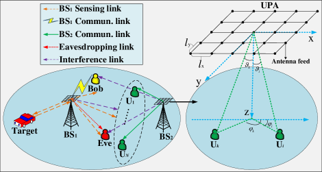
Figure 1: PR-ISAC CRNs architecture.

The remainder of the paper is organized as follows: The channel model, PR-ISAC CRNs architecture, and signal models accompanied by performance indicators are provided in Section II. Section III formulates the optimization problem, and present the corresponding solutions. Numerical results and simulations are provided in Section IV. Section V concludes this paper by summarizing its main message and key remarks.

Notations: Matrices and vectors are denoted as uppercase boldface and lowercase boldface, respectively. ${\left(\cdot\right)^{\rm{H}}}$, ${\mathop{\rm Tr}\nolimits}\left(\cdot\right)$, ${\mathop{\rm rank}\nolimits}\left(\cdot\right)$, and ${\left\|\cdot\right\|_{2}}$ are the Hermitian transpose operation, trace operation, rank operation, and 2-norm operation. ${\mathbb{C}^{x\times y}}$ stands for the 2-dimension complex space. ${{\bf{I}}_{Z}}$ represents the $Z\times Z$ identity matrix, ${{\bf{I}}_{{Z\times 1}}}$ represents the $\left({{Z}\times 1}\right)$-dimension unit vector, $\otimes$ denotes the Kroneker product of two matrices, $\mathcal{O}$ is computational complexity, and ${\left[x\right]^{+}}=\max\left\{{0,x}\right\}$.

II System, Channel, and Signal Models

To facilitate the formulation and solution of the optimization problem, we describe the architecture, Rician-shadowed fading channel, legitimate communication signal and unauthenticated eavesdropping signal in the ISAC, the RSMA-based multicast communication signal, and the sensing signal in the ISAC.

II-A System Model

As shown in Figure 1, in CRNs, there are two sub-networks, namely ISAC as primary network and multicast communications as secondary network. In the primary network, $\rm BS_{1}$ is equipped with $M_{1}$ antennas provides the downlink data transmission service to Bob while sensing the target’s location status information. Meanwhile, Eve, an unauthorized external eavesdropper equipped with a single antenna, attempts to wiretap confidential information that $\rm BS_{1}$ transmits to Bob. In the secondary network, $\rm BS_{2}$ equipped with $M_{2}$ antennas employs the RSMA scheme to provide highly reliable and low-interference downlink data transmission for $N$ users. Obviously, in the PR-ISAC CRNs, the signal transmitted by $\rm BS_{1}$ interferes with $N$ communication users’ received signals, while the signal transmitted by $\rm BS_{2}$ affects both Bob’s and Eve’s signal reception.

II-B Channel Model

In the primary network, a portion of the line of sight (LoS) component is refracted and scattered by buildings and trees, forming the non LoS (NLoS) component that coexists with the LoS component. Therefore, the downlink channel can be modeled as the superposition of a predominant LoS component and a sparse set of single-bounce NLoS components. This situation can be accurately characterized by the Rician-shadowed fading channel model in [42], which is taken into account to capture the statistical characteristics of communication and sensing. Specifically, we have

$$\begin{array}[]{l}{\bf{h}}=\sqrt{\rho\left({{\vartheta_{0}},{\varphi_{0}}}\right)}{\alpha_{\rm{0}}}{{\bf{u}}_{\rm{h}}}\left({{\vartheta_{0}},{\varphi_{0}}}\right)\otimes{{\bf{u}}_{\rm{e}}}\left({{\vartheta_{0}},{\varphi_{0}}}\right)+\\ \displaystyle\frac{1}{{\sqrt{T}}}\sum\nolimits_{t=1}^{T}{\sqrt{\rho\left({{\vartheta_{t}},{\varphi_{t}}}\right)}{\alpha_{t}}{{\bf{u}}_{\rm{h}}}\left({{\vartheta_{t}},{\varphi_{t}}}\right)\otimes{{\bf{u}}_{\rm{e}}}\left({{\vartheta_{t}},{\varphi_{t}}}\right)},\end{array}$$ (1)

where $\rho\left({\vartheta,\varphi}\right)$ is the antenna directivity pattern, ${{\bf{u}}_{\rm{h}}}\left({\vartheta,\varphi}\right)$ and ${{\bf{u}}_{\rm{e}}}\left({\vartheta,\varphi}\right)$ are horizon and elevation steering vectors, respectively, $\alpha_{0}$ and $\alpha_{t}$ are path-loss parameters of the LoS and the $t$-th NLoS components, $\varphi$ and $\vartheta$ are the azimuth and elevation angles of departure, respectively, and $T$ is the number of NLoS components. ${{\bf{u}}_{\rm{h}}}\left({{\vartheta_{t}},{\varphi_{t}}}\right)$ and ${{\bf{u}}_{\rm{e}}}\left({{\vartheta_{t}},{\varphi_{t}}}\right)$ obtained as in (2) and (3), given at the top of this page, where $\eta$ is the phase constant, $l_{\rm x}$ and $l_{\rm y}$ are distances between two adjacent antenna feeds of horizon direction and elevation direction, and ${M_{1}}={M_{{\rm{1,1}}}}\times{M_{{\rm{1,2}}}}$.

$${{\bf{u}}_{\rm{h}}}\left({{\vartheta_{t}},{\varphi_{t}}}\right)={\left[{{e^{-j\eta\left({{M_{{\rm{1}},{\rm{1}}}}-1}\right){2^{-1}}{l_{\rm{x}}}\sin{\vartheta_{t}}\cos{\varphi_{t}}}},\cdots,{e^{j\eta\left({{M_{{\rm{1}},{\rm{1}}}}-1}\right){2^{-1}}{l_{\rm{x}}}\sin{\vartheta_{t}}\cos{\varphi_{t}}}}}\right]^{\rm{T}}},$$ (2)

$${{\bf{u}}_{\rm{e}}}\left({{\vartheta_{t}},{\varphi_{t}}}\right)={\left[{{e^{-j\eta\left({{M_{{\rm{1}},{\rm{2}}}}-1}\right){2^{-1}}{l_{\rm{y}}}\cos{\vartheta_{t}}}},\cdots,{e^{j\eta\left({{M_{{\rm{1}},{\rm{2}}}}-1}\right){2^{-1}}{l_{\rm{y}}}\cos{\vartheta_{t}}}}}\right]^{\rm{T}}},$$ (3)

In what follows, it is necessary to point out that unless otherwise specified, all channels considered are with the magnitudes of their elements following Rician-shadowed distributions by default.

II-C Communication Signal Model

For $\rm BS_{1}$, let ${x_{{\rm{bo}}}}$ and ${x_{{\rm{ta}}}}$ represent the communication signal transmitted to Bob and the sensing signal transmitted to target, respectively. ${{\bf{w}}_{{\rm{bo}}}}\in{\mathbb{C}^{{M_{1}}\times 1}}$ and ${{\bf{w}}_{{\rm{ta}}}}\in{\mathbb{C}^{{M_{1}}\times 1}}$ are the BF vectors of ${x_{{\rm{bo}}}}$ and ${x_{{\rm{ta}}}}$, respectively. Before transmitting ${x_{{\rm{bo}}}}$ and ${x_{{\rm{ta}}}}$, $\rm BS_{1}$ superimposes ${x_{{\rm{bo}}}}$ and ${x_{{\rm{ta}}}}$ together. Thus, the final signal transmitted by $\rm BS_{1}$ can be expressed as

$${{\bf{x}}_{1}}={{\bf{w}}_{{\rm{bo}}}}{x_{{\rm{bo}}}}+{{\bf{w}}_{{\rm{ta}}}}{x_{{\rm{ta}}}}.$$ (4)

Additionally, given that $\rm BS_{2}$ uses the RSMA scheme to implement multicast communications, all signals transmitted by $\rm BS_{2}$ to $N$ communication users can be divided into two parts, i.e., common stream and the private stream, namely $\left\{{z_{\rm 1}^{\rm{c}},z_{\rm 1}^{\rm{p}}}\right\}$, $\left\{{z_{\rm 2}^{\rm{c}},z_{\rm 2}^{\rm{p}}}\right\}$, $\cdots\cdots$, $\left\{{z_{{\rm}N}^{\rm{c}},z_{{\rm},N}^{\rm{p}}}\right\}$, respectively. Then, $N$ common streams, $\left\{{z_{\rm 1}^{\rm{c}},z_{\rm 2}^{\rm{c}},\cdots,z_{\rm\it N}^{\rm{c}}}\right\}$, are extracted, combined, and encoded as the common information, $s_{\rm c}$ via a codebook shared by $N$ communication users. Private streams, $\left\{{z_{\rm 1}^{\rm{p}},z_{\rm 2}^{\rm{p}},\cdots,z_{\rm\it N}^{\rm{p}}}\right\}$, are encoded separately as private information $\left\{{{s_{1}},{s_{2}},\cdots,{s_{N}}}\right\}$, respectively. It is assumed that the signals $x_{\rm bo}$, $x_{\rm ta}$, $s_{\rm c}$, and $s_{n}$ are uncorrelated with zero mean and unit variance. Then, we assume that ${{\bf{o}}_{\rm{c}}}\in{\mathbb{C}^{M_{2}\times 1}}$ and ${{\bf{o}}_{{\it n}}}\in{\mathbb{C}^{M_{2}\times 1}}$ are beamformers of the common information $s_{\rm i,c}$ and the private information of the $n$-th communication user ${s_{n}}$, $n\in\left\{{1,2,\cdots,N}\right\}$, respectively. The signal transmitted by ${\rm BS_{2}}$ can be

$${{\bf{x}}_{2}}={{\bf{o}}_{\rm{c}}}{s_{\rm{c}}}+\sum\nolimits_{n=1}^{N}{{{\bf{o}}_{n}}{s_{n}}}.$$ (5)

Let ${{\bf{h}}_{{\rm{bo}}}}\in{\mathbb{C}^{{M_{1}}\times 1}}$, ${{\bf{h}}_{{\rm{e}}}}\in{\mathbb{C}^{{M_{1}}\times 1}}$, and ${{\bf{h}}_{{n}}}\in{\mathbb{C}^{{M_{1}}\times 1}}$ represent the channels from $\rm BS_{1}$ to Bob, Eve, and the $n$-th user. Likewise, ${{\bf{g}}_{{\rm{bo}}}}\in{\mathbb{C}^{{M_{2}}\times 1}}$, ${{\bf{g}}_{{\rm{e}}}}\in{\mathbb{C}^{{M_{2}}\times 1}}$, and ${{\bf{g}}_{{n}}}\in{\mathbb{C}^{{M_{2}}\times 1}}$ represent the channels from $\rm BS_{2}$ to Bob, Eve, and the $n$-th user. $n_{\rm bo}$, $n_{\rm e}$, and $n_{n}$ are independent and identically distributed complex random Gaussian noises with mean being 0 and variance being $\sigma^{2}$ at Bob, Eve, and $n$-th user. The received signals at Bob, Eve, and $n$-th user are given by

$$\begin{array}[]{*{20}{l}}\displaystyle{{y_{{\rm{bo}}}}={\bf{h}}_{{\rm{bo}}}^{\rm{H}}{{\bf{w}}_{{\rm{bo}}}}{x_{{\rm{bo}}}}+{n_{{\rm{bo}}}}}\\ \quad\;\;\,\displaystyle{+{\bf{h}}_{{\rm{bo}}}^{\rm{H}}{{\bf{w}}_{{\rm{ta}}}}{x_{{\rm{ta}}}}+{\bf{g}}_{{\rm{bo}}}^{\rm{H}}{{\bf{o}}_{\rm{c}}}{s_{\rm{c}}}+\sum\nolimits_{n=1}^{N}{{\bf{g}}_{{\rm{bo}}}^{\rm{H}}{{\bf{o}}_{n}}{s_{n}}},}\end{array}$$ (6)

$$\begin{array}[]{*{20}{l}}\displaystyle{{y_{\rm{e}}}{\rm{=}}{\bf{h}}_{\rm{e}}^{\rm{H}}{{\bf{w}}_{{\rm{bo}}}}{x_{{\rm{bo}}}}+{n_{\rm{e}}}}\\ \displaystyle\quad{+{\bf{h}}_{\rm{e}}^{\rm{H}}{{\bf{w}}_{{\rm{ta}}}}{x_{{\rm{ta}}}}+{\bf{g}}_{\rm{e}}^{\rm{H}}{{\bf{o}}_{\rm{c}}}{s_{\rm{c}}}+\sum\nolimits_{n=1}^{N}{{\bf{g}}_{\rm{e}}^{\rm{H}}{{\bf{o}}_{n}}{s_{n}}},}\end{array}$$ (7)

$$\begin{array}[]{*{20}{l}}\displaystyle{{y_{n}}={\bf{g}}_{n}^{\rm{H}}{{\bf{o}}_{\rm{c}}}{s_{\rm{c}}}+{\bf{g}}_{n}^{\rm{H}}{{\bf{o}}_{n}}{s_{n}}+{n_{n}}}\\ \displaystyle\quad\;+{\sum\nolimits_{k\neq n}{{\bf{g}}_{k}^{\rm{H}}{{\bf{o}}_{k}}{s_{k}}}+{\bf{h}}_{n}^{\rm{H}}{{\bf{w}}_{{\rm{bo}}}}{x_{{\rm{bo}}}}+{\bf{h}}_{n}^{\rm{H}}{{\bf{w}}_{{\rm{ta}}}}{x_{{\rm{ta}}}},}\end{array}$$ (8)

respectively. Since Eve is foreign, unauthorized, and non-cooperative to $\rm BS_{1}$ and $\rm BS_{2}$, they ascertain Eve’s imperfect CSI. As such, we have

$${{\bf{h}}_{\rm{e}}}={{\bf{h}}_{{\rm{es}}}}+{{\bf{h}}_{{\rm{er}}}},$$ (9)

$${{\bf{g}}_{\rm{e}}}={{\bf{g}}_{{\rm{es}}}}+{{\bf{g}}_{{\rm{er}}}},$$ (10)

respectively, where ${{\bf{h}}_{{\rm{es}}}}$ and ${{\bf{g}}_{{\rm{es}}}}$ are the estimated CSIs of the $\rm BS_{1}$-Eve and $\rm BS_{2}$-Eve links, ${{\bf{h}}_{{\rm{er}}}}$ and ${{\bf{g}}_{{\rm{er}}}}$ represent the differences between the real and estimated CSIs of the $\rm BS_{1}$-Eve and $\rm BS_{2}$-Eve links, respectively, of which the 2-norms satisfy

$$0\leq{\left\|{{{\bf{h}}_{{\rm{er}}}}}\right\|_{2}}\leq{{\rm{e}}_{\rm{h}}},$$ (11)

$$0\leq{\left\|{{{\bf{g}}_{{\rm{er}}}}}\right\|_{2}}\leq{{\rm{e}}_{\rm{g}}},$$ (12)

respectively, where ${{\rm{e}}_{\rm{h}}}$ and ${{\rm{e}}_{\rm{g}}}$ are the upper bounds of 2-norms of ${{\bf{h}}_{{\rm{er}}}}$ and ${{\bf{g}}_{{\rm{er}}}}$. To quantify the CSI uncertainty of the $\rm BS_{1}$-Eve link, there exist

$${\left\|{{\bf{h}}_{\rm{e}}^{\rm{H}}{{\bf{w}}_{{\rm{bo}}}}}\right\|_{2}^{2}={\bf{w}}_{{\rm{bo}}}^{\rm{H}}\left({{{\bf{h}}_{{\rm{es}}}}{\bf{h}}_{{\rm{es}}}^{\rm{H}}+{{\bf{\Delta}}_{\rm{h}}}}\right){{\bf{w}}_{{\rm{bo}}}},}$$ (13)

$$\begin{array}[]{l}\left\|{{\bf{h}}_{\rm{e}}^{\rm{H}}{{\bf{w}}_{{\rm{ta}}}}}\right\|_{2}^{2}={\bf{w}}_{{\rm{ta}}}^{\rm{H}}\left({{{\bf{h}}_{{\rm{es}}}}{\bf{h}}_{{\rm{es}}}^{\rm{H}}+{{\bf{\Delta}}_{\rm{h}}}}\right){{\bf{w}}_{{\rm{ta}}}},\end{array}$$ (14)

where ${{\bf{\Delta}}_{\rm{h}}}={{\bf{h}}_{{\rm{es}}}}{\bf{h}}_{{\rm{er}}}^{\rm{H}}+{{\bf{h}}_{{\rm{er}}}}{\bf{h}}_{{\rm{es}}}^{\rm{H}}+{{\bf{h}}_{{\rm{er}}}}{\bf{h}}_{{\rm{er}}}^{\rm{H}}$ is the CSI error matrix of $\rm BS_{1}$-Eve link, and satisfies the compatibility and triangle inequality constraint. Then, we can get a range of values for the 2-norm of ${{\bf{\Delta}}_{\rm{h}}}$, i.e., ${{{\left\|{{{\bf{\Delta}}_{\rm{h}}}}\right\|}_{2}}\leq{\rm{e}}_{\rm{h}}^{\rm{2}}+2{{\rm{e}}_{\rm{h}}}{{\left\|{{{\bf{h}}_{{\rm{er}}}}}\right\|}_{2}}={{\rm{e}}_{{\rm{h}},{\rm{UB}}}}}$, where ${{\rm{e}}_{{\rm{h,UB}}}}$ is the upper bound of 2-norm of ${{\bf{\Delta}}_{\rm{h}}}$. Similarly, we obtain $\left\|{{\bf{g}}_{\rm{e}}^{\rm{H}}{{\bf{o}}_{\rm{c}}}}\right\|_{2}^{2}={\bf{o}}_{\rm{c}}^{\rm{H}}\left({{{\bf{g}}_{{\rm{es}}}}{\bf{g}}_{{\rm{es}}}^{\rm{H}}+{{\bf{\Delta}}_{\rm{g}}}}\right){{\bf{o}}_{\rm{c}}}$ and $\left\|{{\bf{g}}_{\rm{e}}^{\rm{H}}{{\bf{o}}_{n}}}\right\|_{2}^{2}={\bf{o}}_{n}^{\rm{H}}\left({{{\bf{g}}_{{\rm{es}}}}{\bf{g}}_{{\rm{es}}}^{\rm{H}}+{{\bf{\Delta}}_{\rm{g}}}}\right){{\bf{o}}_{n}}$, where ${{\bf{\Delta}}_{\rm{g}}}={{\bf{g}}_{{\rm{es}}}}{\bf{g}}_{{\rm{er}}}^{\rm{H}}+{{\bf{g}}_{{\rm{er}}}}{\bf{g}}_{{\rm{es}}}^{\rm{H}}+{{\bf{g}}_{{\rm{er}}}}{\bf{g}}_{{\rm{er}}}^{\rm{H}}$ is the CSI error matrix of the $\rm BS_{2}$-Eve link, and satisfies the compatibility and triangle inequality constraint. Then, we get a range of values for the 2-norm of ${{\bf{\Delta}}_{\rm{g}}}$, i.e., ${\left\|{{{\bf{\Delta}}_{\rm{g}}}}\right\|_{2}}\leq{\rm{e}}_{\rm{g}}^{\rm{2}}+2{{\rm{e}}_{\rm{g}}}{\left\|{{{\bf{g}}_{{\rm{er}}}}}\right\|_{2}}={{\rm{e}}_{{\rm{g,UB}}}}$, where ${{\rm{e}}_{{\rm{g,UB}}}}$ is the upper bound of 2-norm of ${{\bf{\Delta}}_{\rm{g}}}$.

In the ISAC, the decoding order is (i) sensing and (ii) communication signals. Hence, it is assumed that the channel gain of the sensing signal is greater than that of the communication signal, i.e, $\left\|{{\bf{h}}_{{\rm{bo}}}^{\rm{H}}{{\bf{w}}_{{\rm{bo}}}}}\right\|_{2}^{2}<\left\|{{\bf{h}}_{{\rm{bo}}}^{\rm{H}}{{\bf{w}}_{{\rm{ta}}}}}\right\|_{2}^{2}$ and $\left\|{{\bf{h}}_{{\rm{bo}}}^{\rm{H}}{{\bf{w}}_{{\rm{bo}}}}}\right\|_{2}^{2}<\left\|{{\bf{h}}_{{\rm{bo}}}^{\rm{H}}{{\bf{w}}_{{\rm{ta}}}}}\right\|_{2}^{2}$

The sensing SINR at Bob can be obtained as

$${\gamma_{{\rm{bo,ta}}}}=\frac{{\left\|{{\bf{h}}_{{\rm{bo}}}^{\rm{H}}{{\bf{w}}_{{\rm{ta}}}}}\right\|_{2}^{2}}}{{\left\|{{\bf{h}}_{{\rm{bo}}}^{\rm{H}}{{\bf{w}}_{{\rm{bo}}}}}\right\|_{2}^{2}+\left\|{{\bf{g}}_{{\rm{bo}}}^{\rm{H}}{{\bf{o}}_{\rm{c}}}}\right\|_{2}^{2}+\sum\nolimits_{n=1}^{N}{\left\|{{\bf{g}}_{{\rm{bo}}}^{\rm{H}}{{\bf{o}}_{n}}}\right\|_{2}^{2}}+{\sigma^{2}}}}.$$ (15)

To employ SIC and remove sensing signals and reserve communication signals, the following condition needs to be satisfied: ${\gamma_{{\rm{bo,ta}}}}\geq{\gamma_{{\rm{th}}}}$, where ${\gamma_{{\rm{th}}}}$ is the required SINR threshold for decoding sensing signals successfully. Then, with sensing signals eliminated at Bob, the communication SINR at Bob can be represented as

$${\gamma_{{\rm{bo,bo}}}}=\frac{{\left\|{{\bf{h}}_{{\rm{bo}}}^{\rm{H}}{{\bf{w}}_{{\rm{bo}}}}}\right\|_{2}^{2}}}{{\left\|{{\bf{g}}_{{\rm{bo}}}^{\rm{H}}{{\bf{o}}_{\rm{c}}}}\right\|_{2}^{2}+\sum\nolimits_{n=1}^{N}{\left\|{{\bf{g}}_{{\rm{bo}}}^{\rm{H}}{{\bf{o}}_{n}}}\right\|_{2}^{2}}+{\sigma^{2}}}}.$$ (16)

Similarly, the sensing SINR at Eve is

$${\gamma_{{\rm{e,ta}}}}=\frac{{\left\|{{\bf{h}}_{\rm{e}}^{\rm{H}}{{\bf{w}}_{{\rm{ta}}}}}\right\|_{2}^{2}}}{{\left\|{{\bf{h}}_{\rm{e}}^{\rm{H}}{{\bf{w}}_{{\rm{bo}}}}}\right\|_{2}^{2}+\left\|{{\bf{g}}_{\rm{e}}^{\rm{H}}{{\bf{o}}_{\rm{c}}}}\right\|_{2}^{2}+\sum\nolimits_{n=1}^{N}{\left\|{{\bf{g}}_{\rm{e}}^{\rm{H}}{{\bf{o}}_{n}}}\right\|_{2}^{2}}+{\sigma^{2}}}}.$$ (17)

In contrast to Bob, the Eve is constrained to be failed to decode the target’s message, obtaining the communication signal with the sensing signal interference, and thus degradating the eavesdropping SINR, the following condition needs to be satisfied: ${\gamma_{{\rm{bo,ta}}}}<{\gamma_{{\rm{th}}}}$. Therefore, the communication SINR at Eve can be respectively expressed as

$${\gamma_{{\rm{e,bo}}}}=\frac{{\left\|{{{\bf{h}}_{\rm{e}}}{\bf{w}}_{{\rm{bo}}}^{\rm{H}}}\right\|_{2}^{2}}}{{\left\|{{{\bf{h}}_{\rm{e}}}{\bf{w}}_{{\rm{ta}}}^{\rm{H}}}\right\|_{2}^{2}+\left\|{{{\bf{g}}_{\rm{e}}}{\bf{o}}_{\rm{c}}^{\rm{H}}}\right\|_{2}^{2}+\sum\nolimits_{n=1}^{N}{\left\|{{{\bf{g}}_{\rm{e}}}{\bf{o}}_{n}^{\rm{H}}}\right\|_{2}^{2}}+{\sigma^{2}}}}.$$ (18)

Thus, the security rate is given by ${R_{\rm{S}}}={\left[{{R_{{\rm{bo}}}}-{R_{\rm{e}}}}\right]^{+}}$, with ${R_{{\rm{bo}}}}={\log_{2}}\left({1+{\gamma_{{\rm{bo,bo}}}}}\right)$ and ${R_{\rm{e}}}={\log_{2}}\left({1+{\gamma_{{\rm{e,bo}}}}}\right)$ being the legitimate rate at Bob and eavesdropping rate at Eve.

Meanwhile, $\rm BS_{2}$ provides RSMA-based downlink data transmission to $N$ users. According to RSMA, the common information $s_{\rm c}$ is decoded into a common stream first, and the private information $s_{n}$ is regarded as interference. Then, by applying SIC, the common stream is recoded, pre-encoded, and removed from the received signal. The private information $s_{n}$ of the $n$-th user is decoded into a private stream, and private informations of other users is treated as interference. Consequently, the SINRs of the common and the private streams of the $n$-th user can be respectively expressed as

$${\gamma_{\rm{c}}}=\frac{{\left\|{{\bf{g}}_{n}^{\rm{H}}{{\bf{o}}_{\rm{c}}}}\right\|_{2}^{2}}}{{\sum\nolimits_{n=1}^{N}{\left\|{{\bf{g}}_{n}^{\rm{H}}{{\bf{o}}_{n}}}\right\|_{2}^{2}}+\left\|{{\bf{h}}_{n}^{\rm{H}}{{\bf{w}}_{{\rm{bo}}}}}\right\|_{2}^{2}+\left\|{{\bf{h}}_{n}^{\rm{H}}{{\bf{w}}_{{\rm{ta}}}}}\right\|_{2}^{2}+{\sigma^{2}}}},$$ (19)

$${\gamma_{n}}=\frac{{\left\|{{\bf{g}}_{n}^{\rm{H}}{{\bf{o}}_{n}}}\right\|_{2}^{2}}}{{\sum\nolimits_{j\neq n}{\left\|{{\bf{g}}_{j}^{\rm{H}}{{\bf{o}}_{j}}}\right\|_{2}^{2}}+\left\|{{\bf{h}}_{n}^{\rm{H}}{{\bf{w}}_{{\rm{bo}}}}}\right\|_{2}^{2}+\left\|{{\bf{h}}_{n}^{\rm{H}}{{\bf{w}}_{{\rm{ta}}}}}\right\|_{2}^{2}+\sigma_{n}^{2}}}.$$ (20)

The corresponding common and private stream rates can be respectively given by ${R_{\rm{c}}}={\log_{2}}\left({1+{\gamma_{\rm{c}}}}\right)$ and ${R_{{n}}}={\log_{2}}\left({1+{\gamma_{{n}}}}\right)$.

II-D Sensing Signal Model

Since $\rm BS_{1}$ is fully aware of its own transmit signal ${{\bf{x}}_{1}}$, which is composed of the sensing signal ${{\bf{w}}_{{\rm{ta}}}}{x_{{\rm{ta}}}}$ and the communication signal ${{\bf{w}}_{{\rm{bo}}}}{x_{{\rm{bo}}}}$, ${{\bf{x}}_{1}}$ can be used to detect the target. Meanwhile, sensing is affected by clutter from the environment. Therefore, the echo signal received at $\rm BS_{1}$ can be expressed as

$$\begin{array}[]{l}\displaystyle{{\bf{y}}_{{\rm{b1}}}}=\xi{{\bf{h}}_{{\rm{ta}}}}{\bf{h}}_{{\rm{ta}}}^{\rm{H}}\left({{{\bf{w}}_{{\rm{bo}}}}{x_{{\rm{bo}}}}+{{\bf{w}}_{{\rm{ta}}}}{x_{{\rm{ta}}}}}\right)\\ \displaystyle\quad\;\;\;+{{\bf{I}}_{{M_{1\times 1}}}}{\bf{h}}_{{\rm{cl}}}^{\rm{H}}\left({{{\bf{w}}_{{\rm{bo}}}}{x_{{\rm{bo}}}}+{{\bf{w}}_{{\rm{ta}}}}{x_{{\rm{ta}}}}}\right)+{{\bf{n}}_{{\rm{b1}}}},\end{array}$$ (21)

where ${{\bf{h}}_{{\rm{ta}}}}\in{\mathbb{C}^{{M_{1}}\times 1}}$ is the channel from $\rm BS_{1}$ to the target and ${{\bf{h}}_{{\rm{cl}}}}\in{\mathbb{C}^{{M_{1}}\times 1}}$ is the channel from the environment to $\rm BS_{1}$. Additionally, $\xi$ is the radar cross section (RCS) coefficient with the mean square value being ${\kappa^{2}}$, and ${{\bf{n}}_{{\rm{b1}}}}\sim CN\left({0,{\sigma^{2}}{{\bf{I}}_{{M_{1}}\times 1}}}\right)$ represents the complex random Gaussian noise at $\rm BS_{1}$ with a mean being 0 and a variance being $\sigma^{2}$. We model the clutter from the environment as complex random Gaussian noise with a mean being 0 and a variance being $\sigma^{2}$ [43].

Then, a radar receiver filter vector at $\rm BS_{1}$ is defined as ${{\bf{a}}}\in{\mathbb{C}^{{M_{1}}\times 1}}$, and thus the further processed echo signal and SCNR can be respectively obtained as

$$\begin{array}[]{l}\displaystyle{\bf{a}}_{{\rm{b1}}}^{\rm{H}}{{\bf{y}}_{{\rm{b1}}}}=\xi{\bf{a}}_{{\rm{b1}}}^{\rm{H}}{{\bf{h}}_{{\rm{ta}}}}{\bf{h}}_{{\rm{ta}}}^{\rm{H}}\left({{{\bf{w}}_{{\rm{bo}}}}{x_{{\rm{bo}}}}+{{\bf{w}}_{{\rm{ta}}}}{x_{{\rm{ta}}}}}\right)\\ \displaystyle\qquad\quad\,+{\bf{a}}_{{\rm{b1}}}^{\rm{H}}{{\bf{I}}_{{M_{1}}\times 1}}{\bf{h}}_{{\rm{cl}}}^{\rm{H}}\left({{{\bf{w}}_{{\rm{bo}}}}{x_{{\rm{bo}}}}+{{\bf{w}}_{{\rm{ta}}}}{x_{{\rm{ta}}}}}\right)+{\bf{a}}_{{\rm{b1}}}^{\rm{H}}{{\bf{n}}_{{\rm{b1}}}},\end{array}$$ (22)

$${\gamma_{{\rm{b1}}}}=\frac{{{\kappa^{2}}{{\bf{a}}^{\rm{H}}}{{\bf{h}}_{{\rm{ta}}}}{\bf{h}}_{{\rm{ta}}}^{\rm{H}}\left({{{\bf{w}}_{{\rm{bo}}}}{\bf{w}}_{{\rm{bo}}}^{\rm{H}}+{{\bf{w}}_{{\rm{ta}}}}{\bf{w}}_{{\rm{ta}}}^{\rm{H}}}\right){\bf{h}}_{{\rm{ta}}}^{\rm{H}}{{\bf{h}}_{{\rm{ta}}}}{\bf{a}}}}{{2{\sigma^{2}}{{\bf{a}}^{\rm{H}}}{\bf{a}}}}.$$ (23)

Likewise, to successfully decode the echo signal at $\rm BS_{1}$, the following condition should be satisfied: ${\gamma_{{\rm{b1}}}}\geq{\gamma_{{\rm{th}}}}$.

III Optimization Formulation and Solution

We aim at jointly enhancing the system’s sensing, communication, security, and SEE. To this end, we design a joint BF optimization scheme to reduce the interference exerted on Bob, suppress Eve’s eavesdropping, and improve the sensing accuracy and energy utilization based on RSMA and the constructed green interference. Specifically, our objective is to maximize the SEE of the entire PR-ISAC CRNs. The optimization objective SEE is related to $R_{\rm bo}$, $R_{\rm e}$, and $P_{1}+P_{2}+P_{0}$. Optimization of a reduces $P_{1}$ while $\rm BS_{1}$ can successfully decode the echo signal. Optimization of $\textbf{w}_{\rm bo}$ leads to a larger $R_{\rm bo}$, optimizing $\textbf{w}_{\rm ta}$ can reduce $P_{1}$ and $R_{\rm e}$, $\textbf{o}_{\rm c}$ and $\textbf{o}_{n}$ are optimized to increase the multicast communication rate and reduce $R_{\rm e}$. The optimization problem can be mathematically expressed as

$${\bf{P1}}.\;\mathop{\max}\limits_{{\bf{a}},{{\bf{w}}_{{\rm{bo}}}},{{\bf{w}}_{{\rm{ta}}}},{{\bf{o}}_{\rm{c}}},{{\bf{o}}_{n}}}\frac{{{R_{\rm{S}}}\left({{{\bf{w}}_{{\rm{bo}}}},{{\bf{w}}_{{\rm{ta}}}},{{\bf{o}}_{\rm{c}}},{{\bf{o}}_{n}}}\right)}}{{{P_{1}}\left({{{\bf{w}}_{{\rm{bo}}}},{{\bf{w}}_{{\rm{ta}}}}}\right)+{P_{2}}\left({{{\bf{o}}_{\rm{c}}},{{\bf{o}}_{n}}}\right)+{P_{0}}}}$$ (24a)

$${\rm{s}}{\rm{.t}}\quad{\rm{}}\left\|{{{\bf{w}}_{{\rm{bo}}}}}\right\|_{2}^{2}+\left\|{{{\bf{w}}_{{\rm{ta}}}}}\right\|_{2}^{2}={P_{1}}\leq{P_{{\rm{1,max}}}},$$ (24b)

$$\quad\quad{\rm{}}\left\|{{{\bf{o}}_{\rm{c}}}}\right\|_{2}^{2}+\sum\nolimits_{n=1}^{N}{\left\|{{{\bf{o}}_{n}}}\right\|_{2}^{2}}={P_{2}}\leq{P_{{\rm{2,max}}}},$$ (24c)

$$\quad\quad{R_{\rm{S}}}\geq{I_{\rm{S}}}\,\&\,{R_{\rm{c}}}\geq{I_{\rm{c}}}\,\&\,{R_{n}}\geq{I_{\rm p}},$$ (24d)

$$\quad\quad\left\|{{\bf{h}}_{{\rm{bo}}}^{\rm{H}}{{\bf{w}}_{{\rm{bo}}}}}\right\|_{2}^{2}\leq\left\|{{\bf{h}}_{{\rm{bo}}}^{\rm{H}}{{\bf{w}}_{{\rm{ta}}}}}\right\|_{2}^{2},$$ (24e)

$$\quad\quad\left\|{{\bf{h}}_{\rm{e}}^{\rm{H}}{{\bf{w}}_{{\rm{bo}}}}}\right\|_{2}^{2}\leq\left\|{{\bf{h}}_{\rm{e}}^{\rm{H}}{{\bf{w}}_{{\rm{ta}}}}}\right\|_{2}^{2},$$ (24f)

$$\quad\quad{\rm{}}{\gamma_{{\rm{bo,ta}}}}\geq{\gamma_{{\rm{th}}}}\,\&\,{\gamma_{{\rm{e,ta}}}}<{\gamma_{{\rm{th}}}},$$ (24g)

$$\quad\quad\frac{{{\kappa^{2}}{{\bf{a}}^{\rm{H}}}{{\bf{h}}_{{\rm{ta}}}}{\bf{h}}_{{\rm{ta}}}^{\rm{H}}\left({{{\bf{w}}_{{\rm{bo}}}}{\bf{w}}_{{\rm{bo}}}^{\rm{H}}+{{\bf{w}}_{{\rm{ta}}}}{\bf{w}}_{{\rm{ta}}}^{\rm{H}}}\right){\bf{h}}_{{\rm{ta}}}^{\rm{H}}{{\bf{h}}_{{\rm{ta}}}}{\bf{a}}}}{{2{\sigma^{2}}{{\bf{a}}^{\rm{H}}}{\bf{a}}}}\geq{\gamma_{{\rm{th}}}},$$ (24h)

where (24a) is the optimization objective on SEE maximization. (24b) and (24c) are constraints of $\rm BS_{1}$ and $\rm BS_{2}$ power consumptions, $P_{\rm 1,max}$ and $P_{\rm 2,max}$ are maximums of $P_{1}$ and $P_{2}$, $P_{0}$ is constant circuit power consumption. (24d) are constraints on security rate, common stream rate, and private stream rate, respectively. $I_{\rm S}$, $I_{\rm c}$, and $I_{\rm p}$ are thresholds of security rate, common stream rate, and private stream rate. (24e) and (24f) are constraints on the decoding sequence of the sensing signal and the communication signal. (24g) are constraints that Bob and $\rm BS_{1}$ successfully decode sensing signals and Eve fails to decode its received sensing signal, deemed as interference for Eve. What’s more, we define ${P_{{\rm{sum}}}}={P_{1}}+{P_{2}}+{P_{0}}$.

It can be observed that there is a deep coupling relationship between the variables to be optimized in P1 and the optimization objective and corresponding constraints, which brings notable challenges for effectively and reliably solving P1. To this end, we present an alternative iterative optimization algorithm based on Taylor series expansion, MM, SDP, and SCA, respectively. In particular, we decompose the original non-convex and intractable targeted optimization P1 into three sub-optimization problems. The first sub-optimization problem focuses on the optimization of the echo signal BF vector at $\rm BS_{1}$. The second one considers the optimization of the transmit BF vector at $\rm BS_{1}$. The last one is the optimization of the transmit BF vector at $\rm BS_{2}$. In what follows, it is defined ${{\bf{X}}_{i}}={{\bf{x}}_{i}}{\bf{x}}_{i}^{\rm{H}}$. The fractional form of the objective and the coupled variables a, $\textbf{w}_{\rm bo}$, $\textbf{w}_{\rm ta}$, $\textbf{o}_{\rm c}$, $\textbf{o}_{n}$ render problem (24) intractable. Therefore, we split the original problem into three sub-problems, and propose an alternating optimization scheme to solve it.

III-A Optimization of the Echo Signal BF Vector at $\rm BS_{1}$

To optimize the echo signal BF vector at $\rm BS_{1}$ a, we keep $\textbf{w}_{\rm bo}$, $\textbf{w}_{\rm ta}$, $\textbf{o}_{\rm c}$, and $\textbf{o}_{n}$ fixed, and we present the equivalent form of the constraint (24h) as

$${\rm{}}{\bf{P2.1}}{\rm{.}}\;\mathop{\max}\limits_{\bf{a}}\frac{{{\kappa^{2}}}}{{2{\sigma^{2}}}}\frac{{{{\bf{a}}^{\rm{H}}}\left({{{\bf{H}}_{{\rm{ta-b1}}}}{{\bf{w}}_{{\rm{b1}}}}{\bf{w}}_{{\rm{b1}}}^{\rm{H}}{\bf{H}}_{{\rm{ta-b1}}}^{\rm{H}}}\right){\bf{a}}}}{{{{\bf{a}}^{\rm{H}}}{\bf{a}}}}$$ (25a)

$${\rm{s}}{\rm{.t}}\quad\,(\ref{P1}\rm b)\,\mbox{-}\,(\ref{P1}\rm g).$$ (25b)

where ${{\bf{H}}_{{\rm{ta,b1}}}}={{\bf{h}}_{{\rm{ta}}}}{\bf{h}}_{{\rm{ta}}}^{\rm{H}}\in{\mathbb{C}^{{M_{1}}\times{M_{1}}}}$ and ${{\bf{w}}_{{\rm{b1}}}}=\left[{{{\bf{w}}_{{\rm{bo}}}},{{\bf{w}}_{{\rm{ta}}}}}\right]\in{\mathbb{C}^{{M_{1}}\times 2}}$.

Herein, S is a Hermitian matrix, which can be expressed as

$${{{\bf{S}}^{\rm{H}}}={{\left[{\frac{{{\kappa^{2}}{{\bf{h}}_{{\rm{ta}}}}{\bf{h}}_{{\rm{ta}}}^{\rm{H}}\left({{{\bf{w}}_{{\rm{bo}}}}{\bf{w}}_{{\rm{bo}}}^{\rm{H}}+{{\bf{w}}_{{\rm{ta}}}}{\bf{w}}_{{\rm{ta}}}^{\rm{H}}}\right){{\bf{h}}_{{\rm{ta}}}}{\bf{h}}_{{\rm{ta}}}^{\rm{H}}}}{{2{\sigma^{2}}}}}\right]}^{\rm{H}}}={\bf{S}}}.$$ (26)

We diagonalize the Hermitian matrix S, define the eigenvalue diagonal matrix of S as ${\bf{\tilde{S}}}={\mathop{\rm diag}\nolimits}\left\{{{\lambda_{1}},{\lambda_{2}},\cdots,{\lambda_{{M_{1}}}}}\right\}\in{\mathbb{C}^{{M_{1}}\times{M_{1}}}}$, define the eigenvector matrix of S as ${\bf{Q}}=\left\{{{{\bf{q}}_{1}},{{\bf{q}}_{2}},\cdots,{{\bf{q}}_{{M_{1}}}}}\right\}\in{\mathbb{C}^{{M_{1}}\times{M_{1}}}}$ with ${\bf{Q}}{{\bf{Q}}^{\rm{H}}}={{\bf{I}}_{{M_{1}}\times{M_{1}}}}$. Then, (25) can be rewritten as

$${\rm{}}{\bf{P2.2}}{\rm{.}}\;{\mathop{\max}\limits_{\bf{a}}\frac{{{{\bf{a}}^{\rm{H}}}{\bf{Q\tilde{S}}}{{\bf{Q}}^{\rm{H}}}{\bf{a}}}}{{{{\bf{a}}^{\rm{H}}}{\bf{Q}}{{\bf{Q}}^{\rm{H}}}{\bf{a}}}}}$$ (27a)

$${\rm{s}}{\rm{.t}}\quad\,(\ref{P1}\rm b)\,\mbox{-}\,(\ref{P1}\rm g).$$ (27b)

Besides, let ${\bf{\tilde{Q}}}={{\bf{Q}}^{\rm{H}}}{\bf{a}}={\left\{{{{{\bf{\tilde{q}}}}_{1}},{{{\bf{\tilde{q}}}}_{2}},\cdots,{{{\bf{\tilde{q}}}}_{{M_{1}}}}}\right\}^{\rm{H}}}$. By applying ${\bf{\tilde{Q}}}$ to (27), we obtain

$${\rm{}}{\bf{P2.3}}{\rm{.}}\;{\mathop{\max}\limits_{\bf{a}}\frac{{\sum\nolimits_{j=1}^{{M_{1}}}{{\lambda_{j}}{\bf{\tilde{q}}}_{j}^{2}}}}{{\sum\nolimits_{j=1}^{{M_{1}}}{{\bf{\tilde{q}}}_{j}^{2}}}}}$$ (28a)

$${\rm{s}}{\rm{.t}}\quad\,(\ref{P1}\rm b)\,\mbox{-}\,(\ref{P1}\rm g).$$ (28b)

Then, after defining ${\lambda_{\max}}=\max\left\{{{\lambda_{1}},{\lambda_{2}},\cdots,{\lambda_{{M_{1}}}}}\right\}$ and ${\lambda_{\min}}=\min\left\{{{\lambda_{1}},{\lambda_{2}},\cdots,{\lambda_{{M_{1}}}}}\right\}$, we obtain

$$\frac{{\sum\nolimits_{j=1}^{{M_{1}}}{{\lambda_{j}}{\bf{\tilde{q}}}_{j}^{2}}}}{{\sum\nolimits_{j=1}^{{M_{1}}}{{\bf{\tilde{q}}}_{j}^{2}}}}\leq\frac{{\sum\nolimits_{j=1}^{{M_{1}}}{{\lambda_{\max}}{\bf{\tilde{q}}}_{j}^{2}}}}{{\sum\nolimits_{j=1}^{{M_{1}}}{{\bf{\tilde{q}}}_{j}^{2}}}}=\frac{{{\lambda_{\max}}\sum\nolimits_{j=1}^{{M_{1}}}{{\bf{\tilde{q}}}_{j}^{2}}}}{{\sum\nolimits_{j=1}^{{M_{1}}}{{\bf{\tilde{q}}}_{j}^{2}}}}={\lambda_{\max}},$$ (29)

$$\frac{{\sum\nolimits_{j=1}^{{M_{1}}}{{\lambda_{j}}{\bf{\tilde{q}}}_{j}^{2}}}}{{\sum\nolimits_{j=1}^{{M_{1}}}{{\bf{\tilde{q}}}_{j}^{2}}}}\geq\frac{{\sum\nolimits_{j=1}^{{M_{1}}}{{\lambda_{\min}}{\bf{\tilde{q}}}_{j}^{2}}}}{{\sum\nolimits_{j=1}^{{M_{1}}}{{\bf{\tilde{q}}}_{j}^{2}}}}=\frac{{{\lambda_{\min}}\sum\nolimits_{j=1}^{{M_{1}}}{{\bf{\tilde{q}}}_{j}^{2}}}}{{\sum\nolimits_{j=1}^{{M_{1}}}{{\bf{\tilde{q}}}_{j}^{2}}}}={\lambda_{\min}}.$$ (30)

Finally, (25) can be simplified as

$${\rm{}}{\bf{P2}}{\rm{.}}\;\mathop{\max}\limits_{\bf{a}}\frac{{{{\bf{a}}^{\rm{H}}}{\bf{Sa}}}}{{{{\bf{a}}^{\rm{H}}}{\bf{a}}}}={\lambda_{\max}}$$ (31a)

$${\rm{s}}{\rm{.t}}\quad\,(\ref{P1}\rm b)\,\mbox{-}\,(\ref{P1}\rm g).$$ (31b)

In this case, the optimization variable a is equivalent to the eigenvector corresponding to the maximum eigenvalue of S, i.e., ${\bf{Sa}}={\lambda_{\max}}{\bf{a}}$. We use QR decomposition to compute the maximum of the target optimization, i.e., the maximum eigenvalue of S, and the corresponding eigenvector, i.e., the optimization variable a. The corresponding calculation process is provided in Algorithm 1.

III-B Optimization of the Transmit BF Vectors at $\rm BS_{1}$

For fixed a, $\textbf{o}_{\rm c}$, and $\textbf{o}_{n}$, we optimize $\textbf{w}_{\rm bo}$ and $\textbf{w}_{\rm ta}$ in P1 jointly. The security rate in P1 can be rewritten as

$$\begin{array}[]{l}\displaystyle{R_{\rm{S}}}={R_{\rm{1}}}-{R_{\rm{2}}}+{R_{\rm{3}}}-{R_{\rm{4}}}\\ \displaystyle\quad\;\;={\log_{2}}\left({{\mathop{\rm Tr}\nolimits}\left({{{\bf{H}}_{{\rm{bo}}}}{{\bf{W}}_{{\rm{bo}}}}}\right)+{\alpha_{{\rm{bo}}}}}\right)\\ \displaystyle\quad\;\;-{\log_{2}}\left({{\mathop{\rm Tr}\nolimits}\left({{{\bf{H}}_{\rm{e}}}{{\bf{W}}_{{\rm{bo}}}}}\right)+{\mathop{\rm Tr}\nolimits}\left({{{\bf{H}}_{\rm{e}}}{{\bf{W}}_{{\rm{ta}}}}}\right)+{\alpha_{\rm{e}}}}\right)\\ \displaystyle\quad\;\;+{\log_{2}}\left({{\mathop{\rm Tr}\nolimits}\left({{{\bf{H}}_{\rm{e}}}{{\bf{W}}_{{\rm{ta}}}}}\right)+{\alpha_{\rm{e}}}}\right)-{\log_{2}}\left({{\alpha_{{\rm{bo}}}}}\right),\end{array}$$ (32)

where ${\alpha_{{\rm{bo}}}}={\mathop{\rm Tr}\nolimits}\left({{{\bf{G}}_{{\rm{bo}}}}{{\bf{O}}_{\rm{c}}}}\right)+\sum\nolimits_{n=1}^{N}{{\mathop{\rm Tr}\nolimits}\left({{{\bf{G}}_{{\rm{bo}}}}{{\bf{O}}_{n}}}\right)}+{\sigma^{2}}$, and ${\alpha_{\rm{e}}}={\mathop{\rm Tr}\nolimits}\left({{{\bf{G}}_{\rm{e}}}{{\bf{O}}_{\rm{c}}}}\right)+\sum\nolimits_{n=1}^{N}{{\mathop{\rm Tr}\nolimits}\left({{{\bf{G}}_{\rm{e}}}{{\bf{O}}_{n}}}\right)}+{\sigma^{2}}$ are constants.

Algorithm 1 Optimization of echo signal BF vector at $\rm BS_{1}$.

Require: Given $\textbf{w}_{\rm bo}$, $\textbf{w}_{\rm ta}$, $\textbf{o}_{\rm c}$, and $\textbf{o}_{n}$, and related variables in the defined models.

Ensure: Optimal echo signal BF vector a.

1:Set the mean square value of RCS $\kappa$, iteration threshold $\delta$, $\varepsilon=0$, $\lambda_{0}=0$, $\lambda_{-1}=0$, and tolerance threshold $\delta$;

2:while all constraints in (31b) are satisfied do

3:  repeat

4:   Solve the optimization objective in (31) to obtain

5:      the maximum eigenvalue $\lambda_{\varepsilon}$;

6:   Update ${{\bf{a}}_{\varepsilon}}={\mathop{\rm QR}\nolimits}\left({{\bf{S}},{\lambda_{\varepsilon}}}\right)$;

7:   $\varepsilon=\varepsilon+1$;

8:  until ${\lambda_{\varepsilon}}-{\lambda_{\varepsilon-1}}\leq{\delta}$;

9:end while

10:Calculate optimal echo signal BF vector a at $\rm BS_{1}$ with QR decomposition based on maximum eigenvalue, $\lambda_{\rm max}$;

Algorithm 2 Optimization of the transmit BF vectors at $\rm BS_{1}$.

Require: Given a, $\textbf{o}_{\rm c}$, and $\textbf{o}_{n}$, and related variables in the defined models.

Ensure: Optimal transmit signal BF vectors $\textbf{w}_{\rm bo}$ and $\textbf{w}_{\rm ta}$.

1:Set auxiliary variables $r_{\rm a}$ and $s_{\rm a}$, iteration threshold $\delta$, $\varepsilon=0$, ${\rm SEE}_{0}=0$, and ${\rm SEE}_{-1}=0$;

2:while all constraints in (42b) are satisfied do

3:  Set $i=0$, and initialize ${r_{{\rm a},0,i}}$ and ${s_{{\rm a},0,i}}$;

4:  repeat

5:   $i=i+1$;

6:   Solve the optimization objective in (42) to obtain

7:      maximum ${\rm SEE}=\left({2{r_{\rm{a}}}\sqrt{{R_{{\rm{S}},\max}}\left(r\right)}-r_{\rm{a}}^{2}{P_{{\rm{sum}}}}}\right)$;

8:   Update $\textbf{W}_{{\rm bo},{\varepsilon}}$, $\textbf{W}_{{\rm ta},{\varepsilon}}$, $r_{{\rm a,0},i}$, and $s_{{\rm a,0},i}$;

9:  until ${\rm{SE}}{{\rm{E}}_{\varepsilon}}-{\rm{SE}}{{\rm{E}}_{\varepsilon-1}}\leq{\delta}$;

10:  Obtain solutions $\textbf{W}_{\rm bo}$ and $\textbf{W}_{\rm ta}$;

11:  Set ${{\bf{W}}_{{\rm{bo}},\varepsilon+1}}{\rm{=}}{{\bf{W}}_{\rm{bo}}}$ and ${{\bf{W}}_{{{\rm ta}},\varepsilon+1}}{\rm{=}}{{\bf{W}}_{{\rm ta}}}$;

12:  while ${{\bf{W}}_{{\rm{bo}},\varepsilon+1}}\approx{{\bf{W}}_{{\rm{bo}},\varepsilon}}$, and ${{\bf{O}}_{{{n}},\varepsilon+1}}\approx{{\bf{O}}_{{{n}},\varepsilon}}$ are not satisfied do

13:   $\varepsilon=\varepsilon+1$;

14:  end while

15:end while

16:Employ singular value decomposition (SVD) to $\textbf{W}_{\rm bo,\varepsilon}$ and $\textbf{W}_{\rm ta,\varepsilon}$, and then the transmit signal BF vectors $\textbf{w}_{\rm bo}$ and $\textbf{w}_{\rm ta}$ are ascertained, respectively;

According to the MM, the following equality is satisfied: ${\log_{2}}\left(z\right)\leq\frac{{z-{z_{0}}}}{{{z_{0}}}}+{\log_{2}}\left({{z_{0}}}\right)$, where $z_{0}$ is a specific value of variable $z$. Therefore, the second item and the third item in (32) can be upper-bounded as

$$\begin{array}[]{l}\displaystyle{R_{\rm{2}}}\leq\frac{{{\mathop{\rm Tr}\nolimits}\left({{{\bf{H}}_{\rm{e}}}{{\bf{W}}_{{\rm{bo}}}}}\right)-{\mathop{\rm Tr}\nolimits}\left({{{\bf{H}}_{\rm{e}}}{{\bf{W}}_{{\rm{bo,}}i}}}\right)}}{{{\mathop{\rm Tr}\nolimits}\left({{{\bf{H}}_{\rm{e}}}{{\bf{W}}_{{\rm{bo,}}i}}}\right)+{\mathop{\rm Tr}\nolimits}\left({{{\bf{H}}_{\rm{e}}}{{\bf{W}}_{{\rm{ta}}}}}\right)+{\alpha_{\rm{e}}}}}\\ \displaystyle\quad\,\,\,+\frac{{{\mathop{\rm Tr}\nolimits}\left({{{\bf{H}}_{\rm{e}}}{{\bf{W}}_{{\rm{ta}}}}}\right)-{\mathop{\rm Tr}\nolimits}\left({{{\bf{H}}_{\rm{e}}}{{\bf{W}}_{{\rm{ta,}}j}}}\right)}}{{{\mathop{\rm Tr}\nolimits}\left({{{\bf{H}}_{\rm{e}}}{{\bf{W}}_{{\rm{bo,}}i}}}\right)+{\mathop{\rm Tr}\nolimits}\left({{{\bf{H}}_{\rm{e}}}{{\bf{W}}_{{\rm{ta,}}j}}}\right)+{\alpha_{\rm{e}}}}}\\ \displaystyle\quad\,\,\,+{\log_{2}}\left({{\mathop{\rm Tr}\nolimits}\left({{{\bf{H}}_{\rm{e}}}{{\bf{W}}_{{\rm{bo,}}i}}}\right)+{\mathop{\rm Tr}\nolimits}\left({{{\bf{H}}_{\rm{e}}}{{\bf{W}}_{{\rm{ta,}}j}}}\right)+{\alpha_{\rm{e}}}}\right),\end{array}$$ (33)

and

$$\begin{array}[]{l}\displaystyle{R_{\rm{3}}}\leq\frac{{{\mathop{\rm Tr}\nolimits}\left({{{\bf{H}}_{\rm{e}}}{{\bf{W}}_{{\rm{ta}}}}}\right)-{\mathop{\rm Tr}\nolimits}\left({{{\bf{H}}_{\rm{e}}}{{\bf{W}}_{{\rm{ta,}}i}}}\right)}}{{{\mathop{\rm Tr}\nolimits}\left({{{\bf{H}}_{\rm{e}}}{{\bf{W}}_{{\rm{ta,}}i}}}\right)+{\alpha_{\rm{e}}}}}\\ \displaystyle\quad\,\,\,+{\log_{2}}\left({{\mathop{\rm Tr}\nolimits}\left({{{\bf{H}}_{\rm{e}}}{{\bf{W}}_{{\rm{ta,}}i}}}\right)+{\alpha_{\rm{e}}}}\right),\end{array}$$ (34)

where ${{{\bf{W}}_{{\rm{bo,}}i}}}$ is the $i$-th iteration result of ${{{\bf{W}}_{{\rm{bo}}}}}$, and ${{{\bf{W}}_{{\rm{ta,}}j}}}$ is the $j$-th iteration result of ${{{\bf{W}}_{{\rm{ta}}}}}$. Based on (13) and (14), we obtain the minimum of $R_{2}$ in (35) and the maximum of $R_{3}$ in (36) at the top of this page, where ${{\bf{H}}_{{\rm{e,max}}}}={{\bf{H}}_{{\rm{es}}}}+{\rm{e}}_{\rm{h,UB}}{{\bf{I}}_{{M_{1}}\times{M_{1}}}}$ and ${{\bf{H}}_{{\rm{e,min}}}}={{\bf{H}}_{{\rm{es}}}}-{\rm{e}}_{\rm{h,UB}}{{\bf{I}}_{{M_{1}}\times{M_{1}}}}$.

$$\begin{array}[]{l}\displaystyle{R_{{\rm{2}},{\rm{min}}}}=\frac{{{\rm{Tr}}\left({{{\bf{H}}_{{\rm{e}},{\rm{min}}}}{{\bf{W}}_{{\rm{bo}}}}}\right)-{\rm{Tr}}\left({{{\bf{H}}_{{\rm{e}},{\rm{max}}}}{{\bf{W}}_{{\rm{bo}},i}}}\right)}}{{{\rm{Tr}}\left({{{\bf{H}}_{{\rm{e}},{\rm{max}}}}{{\bf{W}}_{{\rm{bo}},i}}}\right)+{\rm{Tr}}\left({{{\bf{H}}_{{\rm{e}},{\rm{max}}}}{{\bf{W}}_{{\rm{ta}}}}}\right)+{\alpha_{\rm{e}}}}}+\frac{{{\rm{Tr}}\left({{{\bf{H}}_{{\rm{e}},{\rm{min}}}}{{\bf{W}}_{{\rm{ta}}}}}\right)-{\rm{Tr}}\left({{{\bf{H}}_{{\rm{e}},{\rm{max}}}}{{\bf{W}}_{{\rm{ta}},j}}}\right)}}{{{\rm{Tr}}\left({{{\bf{H}}_{{\rm{e}},{\rm{max}}}}{{\bf{W}}_{{\rm{bo}},i}}}\right)+{\rm{Tr}}\left({{{\bf{H}}_{{\rm{e}},{\rm{max}}}}{{\bf{W}}_{{\rm{ta}},j}}}\right)+{\alpha_{\rm{e}}}}}\\ \displaystyle\qquad\quad+{\log_{2}}\left({{\rm{Tr}}\left({{{\bf{H}}_{{\rm{e}},{\rm{min}}}}{{\bf{W}}_{{\rm{bo}},i}}}\right)+{\rm{Tr}}\left({{{\bf{H}}_{{\rm{e}},{\rm{min}}}}{{\bf{W}}_{{\rm{ta}},j}}}\right)+{\alpha_{\rm{e}}}}\right),\end{array}$$ (35)

$${R_{{\rm{3}},{\rm{max}}}}=\frac{{{\rm{Tr}}\left({{{\bf{H}}_{{\rm{e}},{\rm{max}}}}{{\bf{W}}_{{\rm{ta}}}}}\right)-{\rm{Tr}}\left({{{\bf{H}}_{{\rm{e}},{\rm{min}}}}{{\bf{W}}_{{\rm{ta}},i}}}\right)}}{{{\rm{Tr}}\left({{{\bf{H}}_{{\rm{e}},{\rm{min}}}}{{\bf{W}}_{{\rm{ta}},i}}}\right)+{\alpha_{\rm{e}}}}}+{\log_{2}}\left({{\rm{Tr}}\left({{{\bf{H}}_{{\rm{e}},{\rm{max}}}}{{\bf{W}}_{{\rm{ta}},i}}}\right)+{\alpha_{\rm{e}}}}\right).$$ (36)

The maximum $R_{\rm S}$ can be expressed as ${R_{{\rm{S}},\max}}={R_{1}}-{R_{{\rm{2,min}}}}+{R_{{\rm{3,max}}}}-{R_{{\rm{4}}}}$. Then, P1 is transformed into

$${\rm{}}{\bf{P3.1}}{\rm{.}}\;\mathop{\max}\limits_{{{\bf{w}}_{{\rm{bo}}}},{{\bf{w}}_{{\rm{ta}}}}}\frac{{{R_{{\rm{S}},{\rm{max}}}}\left({{{\bf{w}}_{{\rm{bo}}}},{{\bf{w}}_{{\rm{ta}}}}}\right)}}{{{P_{1}}\left({{{\bf{w}}_{{\rm{bo}}}},{{\bf{w}}_{{\rm{ta}}}}}\right)+{P_{2}}+{P_{0}}}}$$ (37a)

$${\rm{s}}{\rm{.t}}\quad\,(\ref{P1}\rm b)\,\mbox{-}\,(\ref{P1}\rm h).$$ (37b)

As shown in (37a), we need to increase $R_{\rm S,max}$ and decrease $P_{1}$ to maximize SEE through optimization of $\textbf{w}_{\rm bo}$ and $\textbf{w}_{\rm ta}$. Given optimization function in (37) is fractional and intractable, with a slack variable $r$ and an auxiliary variable $r_{\rm a}$ introduced, the equivalent sub-optimization of (37) is given by

$${\rm{}}{\bf{P3.2}}{\rm{.}}\,\begin{array}[]{*{20}{l}}{\mathop{\max}\limits_{{{\bf{w}}_{{\rm{bo}}}},{{\bf{w}}_{{\rm{ta}}}},{r_{\rm{a}}}}2{r_{\rm{a}}}\sqrt{{R_{{\rm{S}},\max}}}-r_{\rm{a}}^{2}\left({{P_{1}}+{P_{2}}+{P_{0}}}\right)}\end{array}$$ (38b)

$${\rm{s}}{\rm{.t}}\quad\,(\ref{P1}\rm b)\,\mbox{-}\,(\ref{P1}\rm h),$$ (38c)

$$\quad\quad\,{R_{\rm{S}}}\geq{\log_{2}}\left({1+r}\right).$$ (38d)

Since (38c) is non-convex, we introduce an auxiliary variable $s_{\rm a}$ to transform inequality constraints into equality ones. Then, (38c) can be rewritten as

$$2{s_{\rm{a}}}\sqrt{1+{\gamma_{{\rm{bo}},{\rm{bo}}}}}-s_{\rm{a}}^{2}\left({1+{\gamma_{{\rm{e}},{\rm{bo}}}}}\right)\geq r.$$ (39)

Let us define the $i$-th iteration of ${{\bf{w}}_{\rm{bo}}}$ and ${{\bf{w}}_{\rm ta}}$ are defined as ${{\bf{w}}_{{\rm{bo}},i}}$ and ${{\bf{w}}_{{\rm ta},i}}$; then corresponding approximate matrices are given by

$${{\bf{W}}_{{\rm{bo,}}i}}={{\bf{w}}_{{\rm{bo,}}i}}{\bf{w}}_{\rm{bo}}^{\rm{H}}+{{\bf{w}}_{\rm{bo}}}{\bf{w}}_{{\rm{bo,}}i}^{\rm{H}}-{{\bf{w}}_{{\rm{bo,}}i}}{\bf{w}}_{{\rm{bo,}}i}^{\rm{H}},$$ (40)

$${{\bf{W}}_{{\rm{ta,}}i}}={{\bf{w}}_{{\rm{ta,}}i}}{\bf{w}}_{\rm{ta}}^{\rm{H}}+{{\bf{w}}_{\rm{ta}}}{\bf{w}}_{{\rm{ta,}}i}^{\rm{H}}-{{\bf{w}}_{{\rm{ta,}}i}}{\bf{w}}_{{\rm{ta,}}i}^{\rm{H}}.$$ (41)

Finally, the non-convex targeted optimization P1 can be rewritten in a convex form as follows

$${\rm{}}{\bf{P3}}{\rm{.}}\;\mathop{\max}\limits_{{{\bf{w}}_{{\rm{bo}}}},{{\bf{w}}_{{\rm{ta}}}},{r_{\rm a}},{s_{\rm a}}}2{r_{\rm{a}}}\sqrt{{R_{{\rm{S}},\max}}\left(r\right)}-r_{\rm{a}}^{2}{P_{{\rm{sum}}}}$$ (42a)

$${\rm{s}}{\rm{.t}}\quad\,(\ref{P1}\rm b)\,\mbox{-}\,(\ref{P1}\rm h),and\,(\ref{PB2_C2}).$$ (42b)

Corresponding calculation process is summarized in Algorithm 2.

III-C Optimization of the Transmit BF Vector at $\rm BS_{2}$

For the third sub-optimization, we need to increase $R_{\rm S,max}$ and decrease $P_{2}$ to maximize SEE through optimization of $\textbf{o}_{\rm c}$ and $\textbf{o}_{n}$. For given a, $\textbf{w}_{\rm bo}$, and $\textbf{w}_{\rm ta}$, and then $\textbf{o}_{\rm c}$ and $\textbf{o}_{n}$ are optimized in P1. For the sake of simplicity, we define: ${{\bf{\tilde{H}}}_{{\rm{ta-b1}}}}={{\bf{H}}_{{\rm{ta,b1}}}}{\bf{H}}_{{\rm{ta,b1}}}^{\rm{H}}$, ${{\bf{H}}_{{\rm{bo}}}}={{\bf{h}}_{{\rm{bo}}}}{\bf{h}}_{{\rm{bo}}}^{\rm{H}}$, ${{\bf{H}}_{\rm{e}}}={{\bf{h}}_{\rm{e}}}{\bf{h}}_{\rm{e}}^{\rm{H}}$, ${{\bf{W}}_{{\rm{bo}}}}={{\bf{w}}_{{\rm{bo}}}}{\bf{w}}_{{\rm{bo}}}^{\rm{H}}$, and ${{\bf{W}}_{{\rm{ta}}}}={{\bf{w}}_{{\rm{ta}}}}{\bf{w}}_{{\rm{ta}}}^{\rm{H}}$, respectively. Then, we hold that

$$\mathop{\max}\limits_{{{\bf{h}}_{{\rm{es}}}}}{\rm{Tr}}\left({{{\bf{H}}_{\rm{e}}}{{\bf{W}}_{{\rm{bo}}}}}\right)={\rm{Tr}}\left[{\left({{{\bf{H}}_{{\rm{es}}}}+{\rm{e}}_{\rm{h,UB}}{{\bf{I}}_{{M_{1}}\times{M_{1}}}}}\right){{\bf{W}}_{{\rm{bo}}}}}\right],$$ (43)

$$\mathop{\min}\limits_{{{\bf{h}}_{{\rm{es}}}}}{\rm{Tr}}\left({{{\bf{H}}_{\rm{e}}}{{\bf{W}}_{{\rm{bo}}}}}\right)={\rm{Tr}}\left[{\left({{{\bf{H}}_{{\rm{es}}}}-{\rm{e}}_{\rm{h,UB}}{{\bf{I}}_{{M_{1}}\times{M_{1}}}}}\right){{\bf{W}}_{{\rm{bo}}}}}\right],$$ (44)

where ${{\bf{I}}_{{M_{\rm{1}}}}}$ represents the identity matrix with rank being $M_{1}$.

Proposition 1.

The constraint on the security rate in (24d) can be converted to

$$\left({\tau-1}\right){U_{1}}{U_{2}}\geq\tau{\rm{Tr}}\left[{{{\bf{H}}_{{\rm{bo}}}}{{\bf{W}}_{\rm bo}}}\right]{\rm{Tr}}\left[{{{\bf{H}}_{\rm{e}}}{{\bf{W}}_{\rm bo}}}\right],$$ (45)

$$\begin{array}[]{l}\displaystyle{U_{1}}={\rm{Tr}}\left({{{\bf{H}}_{{\rm{bo}}}}{{\bf{W}}_{{\rm{bo}}}}}\right)+\left({1-\tau}\right){\sigma^{2}}\\ \displaystyle\quad\;\,+\left({1-\tau}\right){\rm{Tr}}\left({{{\bf{G}}_{{\rm{bo}}}}{{\bf{O}}_{\rm{c}}}+{{\bf{G}}_{{\rm{bo}}}}\sum\nolimits_{n=1}^{N}{{{\bf{O}}_{n}}}}\right),\end{array}$$ (46)

$$\begin{array}[]{l}\displaystyle{U_{2}}=\frac{\tau}{{\tau-1}}{\rm{Tr}}\left[{{{\bf{H}}_{\rm{e}}}{{\bf{W}}_{{\rm{bo}}}}}\right]+\sigma_{\rm{e}}^{2}\\ \displaystyle\quad\;\,+{\rm{Tr}}\left[{{{\bf{G}}_{\rm{e}}}{{\bf{O}}_{\rm{c}}}+{{\bf{G}}_{\rm{e}}}\sum\nolimits_{n=1}^{N}{{{\bf{O}}_{n}}}}\right]+{\rm{Tr}}\left({{{\bf{H}}_{\rm{e}}}{{\bf{W}}_{{\rm{ta}}}}}\right),\end{array}$$ (47)

respectively, where $\tau={2^{{I_{\rm{S}}}}}$.

Proof.

For brevity, the proof of proposition 1 is provided to Appendix A. ∎

Proposition 2.

The right part of (45) can be rewritten as

$${\rm{Tr}}\left[{{{\bf{H}}_{{\rm{bo}}}}{{\bf{W}}_{{\rm{bo}}}}}\right]{\rm{Tr}}\left[{{{\bf{H}}_{\rm{e}}}{{\bf{W}}_{{\rm{bo}}}}}\right]{\rm{=Tr}}{\left[{{{\bf{h}}_{{\rm{bo}}}}{\bf{h}}_{\rm{e}}^{\rm{H}}{{\bf{W}}_{{\rm{bo}}}}}\right]^{2}}.$$ (48)

Proof.

Please refer to Appendix B. ∎

Proposition 3.

The following inequality holds:

$${U_{1}}+{U_{2}}\geq{\left\|{\begin{array}[]{*{20}{c}}{2\sqrt{{\tau\mathord{\left/{\vphantom{\tau{\left({\tau-1}\right)}}}\right.\kern-1.2pt}{\left({\tau-1}\right)}}}{\rm{Tr}}\left({{{\bf{h}}_{{\rm{bo}}}}{\bf{h}}_{\rm{e}}^{\rm{H}}{{\bf{W}}_{\rm bo}}}\right)}\\ \displaystyle{-{U_{1}}+{U_{2}}}\end{array}}\right\|_{2}}.$$ (49)

Proof.

Please refer to Appendix C. ∎

Based on (11) and (47), the range value of $U_{2}$ can be expressed as ${U_{2,{\rm{UB}}}}\geq{U_{2}}\geq{U_{2,{\rm{LB}}}}$, where

$$\begin{array}[]{l}\displaystyle{U_{2,{\rm{UB}}}}=\frac{\upsilon}{{\upsilon-1}}{\rm{Tr}}\left[{\left({{{\bf{H}}_{{\rm{es}}}}+{{\rm{e}}_{{\rm{h,UB}}}}{{\bf{I}}_{{M_{1}}\times{M_{1}}}}}\right){{\bf{W}}_{{\rm{bo}}}}}\right]\\ \displaystyle\quad\quad\;\;\,+{\rm{Tr}}\left[{{{\bf{T}}_{\rm{e}}}{{\bf{O}}_{\rm{c}}}+{{\bf{T}}_{\rm{e}}}\sum\nolimits_{n=1}^{N}{{{\bf{O}}_{n}}}}\right]+{\sigma^{2}}\\ \displaystyle\quad\quad\;\;\,+{\rm{Tr}}\left[{\left({{{\bf{H}}_{{\rm{es}}}}+{{\rm{e}}_{{\rm{h,UB}}}}{{\bf{I}}_{{M_{1}}\times{M_{1}}}}}\right){{\bf{W}}_{{\rm{ta}}}}}\right],\end{array}$$ (50)

and

$$\begin{array}[]{l}\displaystyle{U_{2,{\rm{LB}}}}=\frac{\upsilon}{{\upsilon-1}}{\rm{Tr}}\left[{\left({{{\bf{H}}_{{\rm{es}}}}-{{\rm{e}}_{{\rm{h,UB}}}}{{\bf{I}}_{{M_{1}}\times{M_{1}}}}}\right){{\bf{W}}_{{\rm{bo}}}}}\right]\\ \displaystyle\quad\quad\;\;\,+{\rm{Tr}}\left[{{{\bf{T}}_{\rm{e}}}{{\bf{O}}_{\rm{c}}}+{{\bf{T}}_{\rm{e}}}\sum\nolimits_{n=1}^{N}{{{\bf{O}}_{n}}}}\right]+{\sigma^{2}}\\ \displaystyle\quad\quad\;\;\,+{\rm{Tr}}\left[{\left({{{\bf{H}}_{{\rm{es}}}}-{{\rm{e}}_{{\rm{h,UB}}}}{{\bf{I}}_{{M_{1}}\times{M_{1}}}}}\right){{\bf{W}}_{{\rm{ta}}}}}\right].\end{array}$$ (51)

Proposition 4.

Based on (49), (50), and (51), the following inequality holds:

$${U_{1}}+{U_{{\rm{2,LB}}}}\geq{\left\|{\begin{array}[]{*{20}{c}}{2\sqrt{{\tau\mathord{\left/{\vphantom{\tau{\left({\tau-1}\right)}}}\right.\kern-1.2pt}{\left({\tau-1}\right)}}}{\rm{Tr}}\left[{{\bf{\tilde{H}}}{{\bf{W}}_{{\rm{bo}}}}}\right]}\\ {-{U_{1}}+{U_{{\rm{2,UB}}}}}\end{array}}\right\|_{2}},$$ (52)

where ${\bf{\tilde{H}}}={{\bf{h}}_{{\rm{bo}}}}{\bf{h}}_{{\rm{es}}}^{\rm{H}}+{{\rm{e}}_{{\rm{h,UB}}}}{{\bf{I}}_{{M_{1}}\times{M_{1}}}}$.

Proof.

Please refer to Appendix D. ∎

Let $\chi=\left\{{{x_{1}},{x_{2}},{x_{3}},{x_{4}},{x_{5}},{x_{6}},{x_{7}}}\right\}$ be a set of auxiliary variables further introduced, and the equivalent form of P1 can be expressed as

$${\rm{}}{\bf{P4.1}}{\rm{.}}\;\mathop{\max}\limits_{{{\bf{o}}_{\rm{c}}},{{\bf{o}}_{n}},\chi}{x_{1}}\left({{{\bf{o}}_{\rm{c}}},{{\bf{o}}_{n}}}\right)$$ (53a)

$${\rm{s}}{\rm{.t}}\quad{x_{2}}-{x_{3}}-{x_{4}}\geq{x_{1}}{x_{7}},$$ (53b)

$$\quad\quad{\rm{Tr}}\left({{{\bf{W}}_{{\rm{b1}}}}}\right)+{\rm{Tr}}\left({{{\bf{O}}_{{\rm{c,}}n}}}\right)\leq{x_{7}},$$ (53c)

$$\quad\quad{\rm{Tr}}\left({{{\bf{H}}_{{\rm{bo}}}}{{\bf{W}}_{{\rm{b1}}}}}\right)+{\rm{Tr}}\left[{{{\bf{G}}_{{\rm{bo}}}}{{\bf{O}}_{{\rm{c,}}n}}}\right]\geq\left({{2^{{x_{2}}}}-1}\right){\sigma^{2}},$$ (53d)

$$\quad\quad{\rm{Tr}}\left[{{{\bf{G}}_{{\rm{bo}}}}{{\bf{O}}_{{\rm{c,}}n}}}\right]\leq\left({{2^{{x_{3}}}}-1}\right){\sigma^{2}},$$ (53e)

$$\quad\quad{\rm{Tr}}\left[{\left({{{\bf{G}}_{{\rm{es}}}}+{{\rm{e}}_{{\rm{g}},{\rm{UB}}}}{{\bf{I}}_{{M_{2}}\times{M_{2}}}}}\right){{\bf{O}}_{{\rm{c,}}n}}}\right]\leq\left({{2^{{x_{6}}}}-1}\right){\sigma^{2}},$$ (53f)

$$\quad\quad{\rm{Tr}}\left[{{{\bf{G}}_{{\rm{es,min}}}}{{\bf{O}}_{{\rm{c,}}n}}}\right]+{\rm{Tr}}\left[{{{\bf{H}}_{{\rm{es,min}}}}{{\bf{W}}_{{\rm{b1}}}}}\right]\geq\left({{2^{{x_{5}}}}-1}\right){\sigma^{2}},$$ (53g)

$$\quad\quad-\left({{2^{{I_{\rm{c}}}}}-1}\right)f\left({{{\bf{O}}_{n}}}\right){\rm{+Tr}}\left({{{\bf{G}}_{n}}{{\bf{O}}_{\rm{c}}}}\right)\geq 0,$$ (53h)

$$\quad\quad-\left({{2^{{I_{\rm{p}}}}}-1}\right)f\left({{{\bf{O}}_{j}}}\right){\rm{+Tr}}\left({\sum\nolimits_{n=1}^{N}{{{\bf{G}}_{n}}{{\bf{O}}_{n}}}}\right)\geq 0,$$ (53i)

$$\quad\quad{x_{5}}-{x_{6}}\leq{x_{4}},$$ (53j)

$$\quad\quad{\rm rank}\left({{{\bf{W}}_{{\rm{b1}}}}}\right)={\rm rank}\left({{{\bf{O}}_{\rm{c}}}}\right)={\rm rank}\left({{{\bf{O}}_{n}}}\right)=1,$$ (53k)

$$\quad\quad(\ref{pro4-1}),(\ref{P1}\rm b),(\ref{P1}\rm c),$$ (53l)

where $f\left({{{\bf{O}}_{n}}}\right)=\left[{{\rm{Tr}}\left({\sum\nolimits_{n=1}^{N}{{{\bf{G}}_{n}}{{\bf{O}}_{n}}}}\right)+{\rm{Tr}}\left({{{\bf{H}}_{n}}{{\bf{W}}_{{\rm{b1}}}}}\right)+\sigma_{n}^{2}}\right]$ and ${{\bf{O}}_{{\rm{c,}}n}}={{\bf{O}}_{\rm{c}}}+\sum\nolimits_{n=1}^{N}{{{\bf{O}}_{n}}}$. Notice that (53b) is non-convex; thus another variable $x_{8}$ is provided to convert (53b) into ${x_{2}}-{x_{3}}-{x_{4}}\geq{x_{8}^{2}}$ and $f\left({{x_{7}},{x_{8}}}\right)=x_{1}^{-1}x_{7}^{-1}x_{8}^{2}\geq 1$, which leads to

$$\frac{{{x_{2}}-{x_{3}}-{x_{4}}+1}}{2}\geq{\left\|{\begin{array}[]{*{20}{c}}\displaystyle{\frac{{{x_{2}}-{x_{3}}-{x_{4}}-1}}{2}}\\ \displaystyle x_{8}\end{array}}\right\|_{2}}.$$ (54)

Proposition 5.

For fixed $x_{7}$ and $x_{8}$, $x_{7,0}$ and $x_{8,0}$, taken into account, the following inequality holds:

$$2{x_{7,0}}{x_{8,0}}{x_{8}}\geq x_{7,0}^{2}{x_{1}}+x_{8,0}^{2}{x_{7}}.$$ (55)

Proof.

Please refer to Appendix E. ∎

Derivation of (55) enables (53e) and (53f) to be respectively expressed as convex forms as follows:

$$\begin{array}[]{l}\displaystyle{\rm{Tr}}\left[{{{\bf{G}}_{{\rm{bo}}}}\left({{{\bf{O}}_{\rm{c}}}+{{\sum\nolimits_{n=1}^{N}{\bf{O}}}_{n}}}\right)}\right]\leq\\ \displaystyle{\sigma^{2}}\left[{{2^{{x_{3,0}}}}\left({{x_{3}}\ln 2-{x_{3,0}}\ln 2+1}\right)-1}\right],\end{array}$$ (56)

$$\begin{array}[]{l}\displaystyle{\rm{Tr}}\left[{\left({{{\bf{G}}_{{\rm{es}}}}+{{\rm{e}}_{{\rm{g,UB}}}}{{\bf{I}}_{{M_{2}}\times{M_{2}}}}}\right)\left({{{\bf{O}}_{\rm{c}}}+\sum\nolimits_{n=1}^{N}{{{\bf{O}}_{n}}}}\right)}\right]\\ \displaystyle\leq{\sigma^{2}}\left[{{2^{{x_{6,0}}}}\left({{x_{6}}\ln 2-{x_{6,0}}\ln 2+1}\right)-1}\right].\end{array}$$ (57)

Let us define the $i$-th iteration of ${{\bf{o}}_{\rm{c}}}$ and ${{\bf{o}}_{n}}$ are defined as ${{\bf{o}}_{{\rm{c}},i}}$ and ${{\bf{o}}_{n,i}}$. Then, the corresponding approximate matrices can be obtained as ${{\bf{O}}_{{\rm{c,}}i}}={{\bf{o}}_{{\rm{c,}}i}}{\bf{o}}_{\rm{c}}^{\rm{H}}+{{\bf{o}}_{\rm{c}}}{\bf{o}}_{{\rm{c,}}i}^{\rm{H}}-{{\bf{o}}_{{\rm{c,}}i}}{\bf{o}}_{{\rm{c,}}i}^{\rm{H}}$ and ${{\bf{O}}_{n,i}}={{\bf{o}}_{n,i}}{\bf{o}}_{n}^{\rm{H}}+{{\bf{o}}_{n}}{\bf{o}}_{n,i}^{\rm{H}}-{{\bf{o}}_{n,i}}{\bf{o}}_{n,i}^{\rm{H}}$. Finally, the non-convex targeted optimization P1 can be rewritten in a convex-form as

$${\rm{}}{\bf{P4}}.\;\mathop{\max}\limits_{{{\bf{o}}_{\rm{c}}},{{\bf{o}}_{n}},\chi}{x_{1}}$$ (58a)

$${\rm{s}}{\rm{.t}}\quad(\ref{P1}\rm b),(\ref{P1}\rm c),(\ref{PB1}\rm c),(\ref{PB1}\rm d),(\ref{PB1}\rm g)~(\ref{PB1}\rm k),$$ (58b)

$$\quad\quad(\ref{pro4-1}),(\ref{specific_value}),(\ref{PB1_f_convex}).$$ (58c)

The calculation process of (58) is presented in Algorithm 3. Finally, the complete algorithm for solving (24) is outlined in Algorithm 4, where Algorithms 1-3 are alternately executed in each iteration.

Algorithm 3 Optimization of the transmit BF vectors at $\rm BS_{2}$.

Require: Given a, $\textbf{w}_{\rm bo}$, and $\textbf{w}_{\rm ta}$, and related variables in the defined models.

Ensure: Optimal transmit signal BF vectors $\textbf{o}_{\rm c}$, and $\textbf{o}_{n}$.

1:Set a set of auxiliary variables $\chi$ and $x_{8}$, iteration threshold $\delta$, $\varepsilon=0$, ${\rm SEE}_{0}=0$, and ${\rm SEE}_{-1}=0$;

2:Set positive values ${\rm e_{h}}$, ${\rm e_{g}}$, ${\rm e_{\rm h,UB}}$, ${\rm e_{\rm g,UB}}$, ${I_{\rm{S}}}$, ${I_{\rm{c}}}$, ${I_{\rm{p}}}$, $P_{\rm 1,max}$, and $P_{\rm 2,max}$;

3:Initialize $\textbf{O}_{\rm c,\varepsilon}$ and $\textbf{O}_{n,\varepsilon}$ to satisfy constraints in (58b) and (58c);

4:while all constraints in (58b) and (58c) are satisfied do

5:  Set $i=0$, and initialize ${x_{2,0,i}}$, ${x_{6,0,i}}$, ${x_{7,0,i}}$, and ${x_{8,0,i}}$;

6:  repeat

7:   $i=i+1$;

8:   Solve the optimization objective in (58) to obtain

9:   maximum SEE;

10:   Update $\textbf{O}_{\rm c,{\varepsilon}}$, $\textbf{O}_{n,\varepsilon}$, ${x_{2,0,i}}$, ${x_{6,0,i}}$, ${x_{7,0,i}}$, and ${x_{8,0,i}}$;

11:  until ${\rm{SE}}{{\rm{E}}_{\varepsilon}}-{\rm{SE}}{{\rm{E}}_{\varepsilon-1}}\leq{\delta}$;

12:  Obtain solutions $\textbf{O}_{\rm c}$ and $\textbf{O}_{n}$;

13:  Set ${{\bf{O}}_{{\rm{c}},\varepsilon+1}}{\rm{=}}{{\bf{O}}_{\rm{c}}}$ and ${{\bf{O}}_{{{n}},\varepsilon+1}}{\rm{=}}{{\bf{O}}_{{n}}}$;

14:  while ${{\bf{O}}_{{\rm{c}},\varepsilon+1}}\approx{{\bf{O}}_{{\rm{c}},\varepsilon}}$, and ${{\bf{O}}_{{{n}},\varepsilon+1}}\approx{{\bf{O}}_{{{n}},\varepsilon}}$ are not satisfied do

15:   $\varepsilon=\varepsilon+1$;

16:  end while

17:end while

18:Employ SVD to $\textbf{O}_{\rm c,\varepsilon}$ and $\textbf{O}_{n,\varepsilon}$, and then the transmit signal BF vectors $\textbf{o}_{\rm c}$ and $\textbf{o}_{n}$ are ascertained, respectively;

Algorithm 4 Optimization of the SEE in (24) based on Algorithms 1, 2, and 3.

Require: Initialization values of a, $\textbf{w}_{\rm bo}$, $\textbf{w}_{\rm ta}$, $\textbf{o}_{\rm c}$, and $\textbf{o}_{n}$, and related variables in the defined models, the number of iterations $\varepsilon$, and tolerance threshold $\delta$, respectively.

Ensure: BF vectors a, $\textbf{w}_{\rm bo}$, $\textbf{w}_{\rm ta}$, $\textbf{o}_{\rm c}$, and $\textbf{o}_{n}$, respectively.

1:repeat

2:  Carry out Algorithm 1 to obtain $\textbf{a}_{\varepsilon+1}$ with $\textbf{w}_{\rm bo,\varepsilon}$,

3:  $\textbf{w}_{\rm ta,\varepsilon}$, $\textbf{o}_{\rm c,\varepsilon}$, and $\textbf{o}_{n,\varepsilon}$;

4:  Carry out Algorithm 2 to obtain $\textbf{w}_{\rm ta,\varepsilon+1}$ and $\textbf{o}_{\rm c,\varepsilon+1}$

5:  with $\textbf{a}_{\varepsilon+1}$, $\textbf{o}_{\rm c,\varepsilon}$, and $\textbf{o}_{n,\varepsilon}$;

6:  Carry out Algorithm 3 to obtain $\textbf{o}_{\rm c,\varepsilon+1}$ and $\textbf{o}_{n,\varepsilon+1}$

7:  with $\textbf{a}_{\varepsilon+1}$, $\textbf{w}_{\rm ta,\varepsilon+1}$, and $\textbf{o}_{\rm c,\varepsilon+1}$;

8:  $\varepsilon=\varepsilon+1$;

9:until Variation of adjacent iteration results is less than $\delta$;

10:Employ QR decomposition to obtain echo signal BF vector a, employ SVD to $\textbf{W}_{\rm bo,\varepsilon}$, $\textbf{W}_{\rm ta,\varepsilon}$, $\textbf{O}_{\rm c,\varepsilon}$, and $\textbf{O}_{n,\varepsilon}$, and then the transmit signal BF vectors $\textbf{w}_{\rm bo}$, $\textbf{w}_{\rm ta}$, $\textbf{o}_{\rm c}$, and $\textbf{o}_{n}$ are ascertained, respectively;

III-D Complexity analysis of Algorithm 4

For Algorithm 4, there exist $M_{1}^{2}+M_{2}^{2}\left({N+1}\right)+1$ original variables, $\left({N+6}\right)$ slack variables, 2 $M_{1}$-size linear matrix inequality (LMI) constraints, $(N+1)$ $M_{2}$-size LMI constraints, $(N+8)$ 1-size LMI constraints, and $(N+1)$ 3-size SOC constraints. Therefore, the computational complexity of Algorithm 4 is given in (59) at the top of the next page, where $D={M_{1}^{2}+\left({N+1}\right)M_{2}^{2}+\left({N+7}\right)}$.

$${\cal O}\left\{{\sqrt{2{M_{1}}+\left({N+1}\right){M_{2}}+\left({N+8}\right)}D\left[{M_{1}^{2}\left({{M_{1}}+D}\right)+\left({N+1}\right)M_{2}^{2}\times\left({{M_{2}}+D}\right)+\left({N+8}\right)\left({1+D}\right)+3\left({N+1}\right)+{D^{2}}}\right]}\right\},$$ (59)

IV Numerical Results and Discussions

In this section, Monte Carlo simulations are performed to illustrate the effectiveness of the presented PR-ISAC CRNs and the BF optimization scheme. The key simulation parameters are set as: The bandwidth $f_{\rm m}$ = 80 MHz, the carrier frequency $f_{\rm c}$= 18 GHz, the coverage region of a cell $r$ = 120 m, numbers of transmit antennas $M_{1}$=12, $M_{2}$=12, number of communication users $N$=4, thresholds of security rate, common and private stream rates, decoding sensing SINR $I_{\rm S}$=1 bit/s/Hz, $I_{\rm c}$=1 bit/s/Hz, $I_{\rm p}$=1 bit/s/Hz, and $\gamma_{\rm th}$=0.5, noise power at $\rm BS_{1}$, Bob, Eve, $n$-th user $\sigma^{2}$=-80 dBmW, maximum transmit power at $\rm BS_{1}$ and $\rm BS_{2}$ $P_{\rm 1,max}$=10 dBW and $P_{\rm 2,max}$=10 dBW, respectively. The rest of this section is structured as: Firstly, we show the convergence performance of Algorithm 4. Next, the sensing SCNRs realized by different echo signal BF vector schemes are illustrated. Effects of different multiple access schemes on the security, power, and SEE of the PR-ISAC CRNs are provided. We give the realizable SEE under different Eve’s CSI uncertainty parameters. We compare the achievable SEEs under different transmit signal BF optimization schemes. Finally, we provide the common and private stream beampatterns based on RSMA.

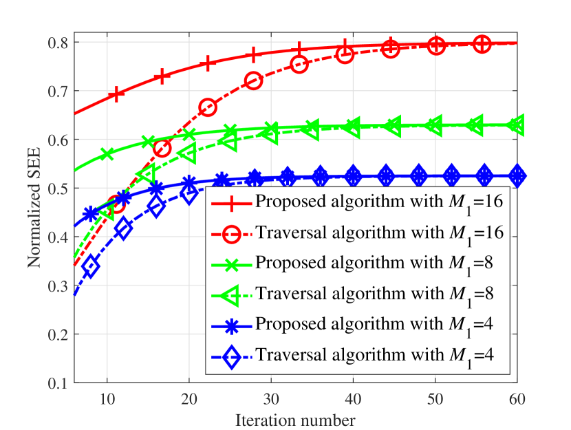
Figure 2: SEE v.s. iteration number for different $M_{1}$.

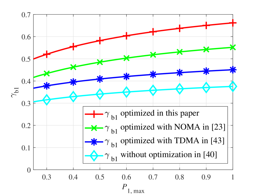
Figure 3: $\gamma_{\rm b1}$ v.s. $P_{\rm 1,max}$ for different optimization schemes.

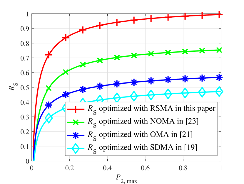
Figure 4: $R_{\rm S}$ v.s. $P_{\rm 2,max}$ for different multiple access schemes.

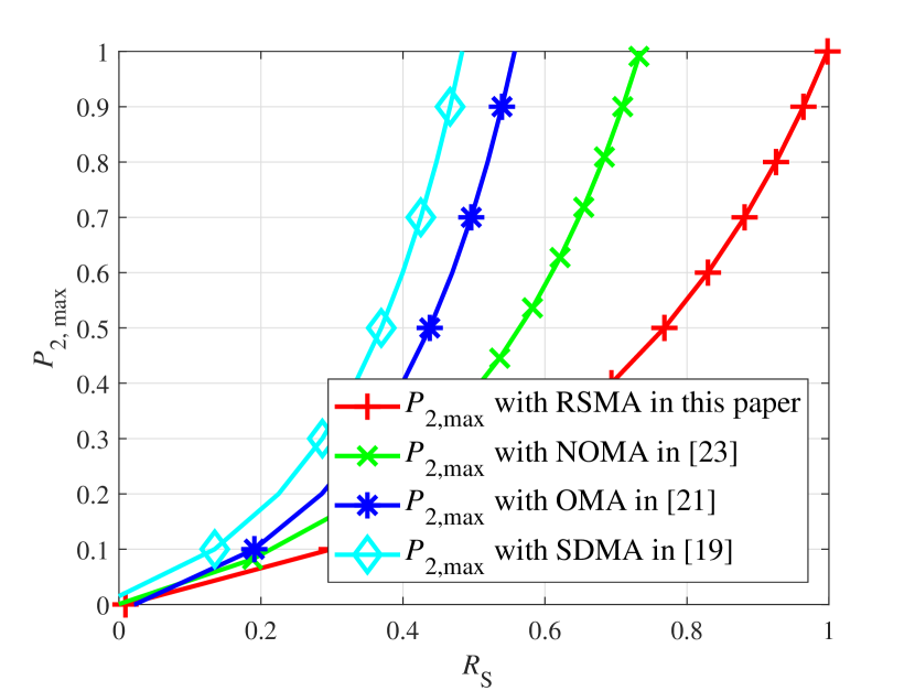
Figure 5: $P_{\rm 2,max}$ v.s. $R_{\rm S}$ for different multiple access schemes.

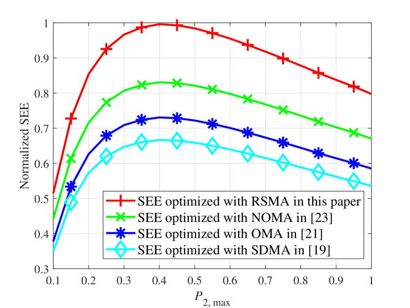
Figure 6: SEE v.s. $P_{\rm 2,max}$ for different multiple access schemes.

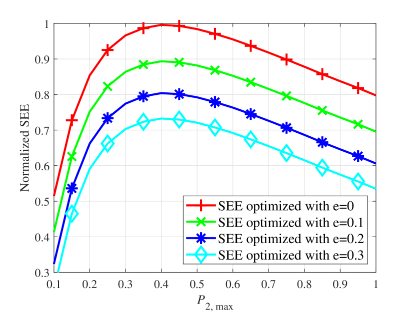
Figure 7: SEE v.s. $P_{\rm 2,max}$ for different CSI uncertainty parameters.

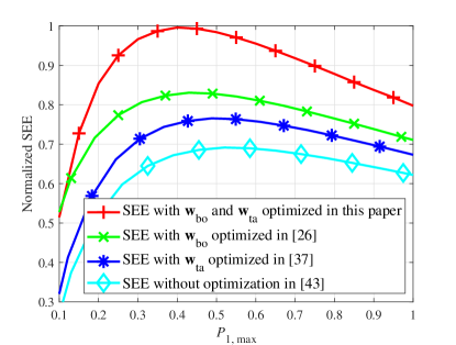
Figure 8: SEE v.s. $P_{\rm 1,max}$ for different transmit BF optimization schemes at $\rm BS_{1}$.

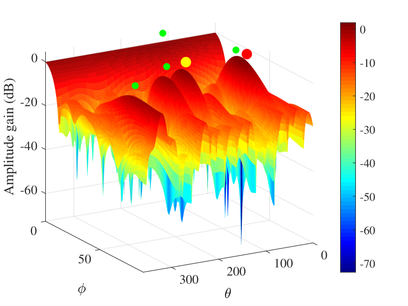
Figure 9: 3D BF pattern of the common stream.

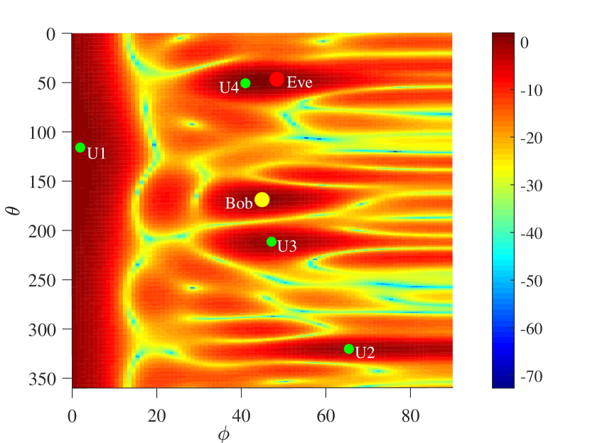
Figure 10: 2D BF pattern of the common stream.

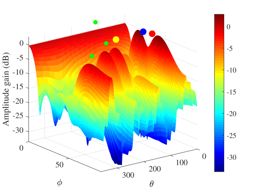
Figure 11: 3D BF pattern of the private stream.

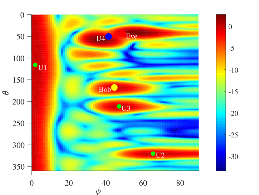
Figure 12: 2D BF pattern of the private stream.

The convergence performance of the SEE improvement in the PR-ISAC CRNs is shown by the solid line in Fig. 3, and the traversal algorithm is depicted by the dashed line in contrast. For a fixed $M_{1}$, the SEE gradually increases with the increase of the number of iterations. After an acceptable number of iterations, SEE converges. For a given number of iterations, SEE increases gradually with the increase of $M_{1}$, since the transmit power carried by a single antenna is constant. The greater $M_{1}$ is, the greater the maximum transmit power becomes, which is translated to an increase of the spatial degrees of freedom and BF design accuracy and efficiency, leading to a greater $R_{\rm S}$ for a fixed transmit power. Then, SEE also increases. As $M_{1}$ increases, the number of iterations required to solve the SEE gradually increases. This is because as $M_{1}$ increases, the computational complexity of the solution also increases; thus the number of iterations increases. For Algorithm 4 and traversal algorithm, as $M_{1}$ increases, the numbers of iterations required to achieve convergence are 24, 30, 39, and 30, 40, and 52, respectively. Obviously, compared with the traversal algorithm, under similar reliability condition and for fixed $M_{1}$, Algorithm 4 requires fewer iterations to achieve convergence, achieving better convergence performance and effectiveness.

In Fig. 3, we show the relationship between $\gamma_{\rm b1}$ and $P_{\rm 1,max}$ under different BF optimization schemes. It can be seen that under the same BF scheme, $\gamma_{\rm b1}$ increases with the increase of $P_{\rm 1,max}$, since the signal power received by the target and reflected to $\rm BS_{1}$ increases with the increase of $P_{\rm 1,max}$ for a given RCS. Meanwhile, the clutter power and noise power in the environment are relatively stable, and thus $\gamma_{\rm b1}$ enhances. In addition, the proposed RSMA-based BF scheme outperforms NOMA in [23], TDMA in [43], and non-optimized echo signal in [40]. This is because the proposed SEE BF optimization scheme continuously receives the echo signal in the time dimension, optimizes the BF vector of the echo signal in the space dimension, and simultaneously uses the sensing signal and the communication signal for sensing the target in the power dimension. However, the other three schemes either neglect to optimize the BF vector of the echo signal, or do not continuously or stably receive the target information, or only use the sensing signal for target identification. Therefore, the proposed multi-BF optimization scheme outperforms the contributions of [23, 43, 40] in terms of sensing.

Fig. 5 illustrates the relationship between $R_{\rm S}$ and $P_{\rm 2,max}$ under four different multiple access schemes. It is obvious that for a fixed multiple access scheme, $R_{\rm S}$ increases as $P_{\rm 2,max}$ increases. This is because the multiple-access-based BF realizes that $\rm BS_{2}$ accounts for the downlink transmission services for $N$ users, while increasing the interference power towards Eve and reducing the interference to Bob. Therefore, with the increase of $P_{\rm 2,max}$, Bob is affected by relatively limited interference, and the change of Bob’s receiving SINR is small, but the interference at Eve is significantly increased, and Eve’s eavesdropping SINR also significantly deteriorates, leading to the improvement of $R_{\rm S}$. Besides, given the fixed $P_{\rm 2,max}$, the RSMA scheme adopted in this paper has a superior $R_{\rm S}$ to NOMA [23], OMA [21], and SDMA [19].

Fig. 5 depicts the relationship between $P_{\rm 2,max}$ and $R_{\rm S}$ for four different multiple access schemes. It is obvious that, for a given multiple access scheme, $P_{\rm 2,max}$ increases gradually as $R_{\rm S}$ increases. This is because the deterioration effect of green interference on Eve’s eavesdropping channel is more powerful than that on Bob’s side. Therefore, a higher $R_{\rm S}$ requires a larger $P_{\rm 2,max}$. However, with the increase of $R_{\rm S}$, the power consumption also increases, since $P_{\rm 2,max}$ is an exponential function of $R_{\rm S}$. This improvement is evident in a certain power range, rather than in the entire power range. Meanwhile, for a given $R_{\rm S}$, $P_{\rm 2,max}$ required for SDMA, OMA, NOMA, and RSMA decreases successively, because the RSMA rationalizes common and private streams to meet different needs with utilizing interference and cutting down power budget, which neither NOMA nor SDMA can do.

Fig. 7 presents the relationship between SEE and $P_{\rm 2,max}$ under different multiple access schemes. Under the same multiple access scheme, with the increase of $P_{\rm 2,max}$, SEE shows a change process of first increasing and then decreasing. This phenomenon is reasonable and based on the definition of SEE [44]. The second derivative of SEE with respect to $P_{\rm 2,max}$ is less than 0, implying SEE is a convex function of $P_{\rm 2,max}$. For a given $P_{\rm 2,max}$, RSMA obtains the best SEE among four multiple access schemes, as presented in Figs. 5 and 5.

Fig. 7 demonstrates the relationship between SEE and $P_{\rm 2,max}$ under different CSI uncertainty parameters. Herein, we define ${\rm{e}}={{{{\rm{e}}_{\rm{h}}}}\mathord{\left/{\vphantom{{{{\rm{e}}_{\rm{h}}}}{{{\left\|{{{\bf{h}}_{{\rm{es}}}}}\right\|}_{2}}}}}\right.\kern-1.2pt}{{{\left\|{{{\bf{h}}_{{\rm{es}}}}}\right\|}_{2}}}}={{{{\rm{e}}_{\rm{g}}}}\mathord{\left/{\vphantom{{{{\rm{e}}_{\rm{g}}}}{{{\left\|{{{\bf{g}}_{{\rm{es}}}}}\right\|}_{2}}}}}\right.\kern-1.2pt}{{{\left\|{{{\bf{g}}_{{\rm{es}}}}}\right\|}_{2}}}}$ to quantitatively characterize the uncertainty of the channel estimation. For a given $P_{\rm 2,max}$, SEE increases with the decrease of e. The smaller e is, the more accurate and reliable the channel estimation is, and the closer the calculation result is to the theoretical upper bound. The smaller the uncertainty of the Eve’s CSI estimation is, the better knowledge of the Eve’s CSI characteristics $\rm BS_{1}$ and $\rm BS_{2}$ has, and the stronger the suppression effect of BF optimization for Eve’s channel is, improving $R_{\rm S}$ and SEE.

Fig. 8 presents the relationship between SEE and $P_{\rm 1,max}$ under different transmit BF optimization schemes. For a fixed multiple access scheme, as $P_{\rm 1,max}$ increases, the SEE shows a change process of first increasing and then decreasing. The effect of $P_{\rm 1,max}$ on SEE can be referred to that of $P_{\rm 2,max}$ on SEE. For a given $P_{\rm 1,max}$, compared with the optimization of $\textbf{w}_{\rm bo}$ in [26], optimization of $\textbf{w}_{\rm ta}$ in [37], and no optimization in [43], the proposed joint optimization of $\textbf{w}_{\rm bo}$ and $\textbf{w}_{\rm ta}$ achieves a higher SEE. Optimization of $\textbf{w}_{\rm ta}$ transforms the harmful interference that affects communication into the green interference that affects eavesdropping with a smaller eavesdropping rate. Optimization of $\textbf{w}_{\rm bo}$ improves the signal quality received by Bob and $R_{\rm S}$. Finally, the proposed joint optimization of $\textbf{w}_{\rm bo}$ and $\textbf{w}_{\rm ta}$ fully demonstrates the advantage in enhancing SEE compared to schemes in [26, 37, 43].

In Figs. 10, 10, 12, and 12, yellow, red, green, and blue dots are positions for Bob, Eve, users, and the user wanting this private stream. Figs. 10 and 10 depict three-dimensional (3D) and two-dimensional (2D) beampatterns of the common stream. There are 4 significant and relatively close amplitude gains with values greater than $\rm 0\,dB$. This is because $\rm BS_{2}$ serves 4 communication users, all of whom require the common stream. Therefore, the amplitude gain of the common stream for 4 users is greater than $\rm 0\,dB$, ensuring that the power of the transmit common stream gets amplified. On the other hand,, amplitude gains of common stream transmitted to Bob and Eve is close to $\rm 0\,dB$. In summary, the optimization of $\textbf{o}_{\rm c}$ in this paper improves the signal power received by each user, and overcomes the fading problem in the signal transmission process. Therefore, each user obtains the common stream reliably while the interference from the common stream exerted on the signal reception of Bob and Eve is limited.

Figs. 12 and 12 illustrate 3D and 2D beampatterns of the private stream. In Figs. 12 and 12, it can be found that among 6 amplitude gains, the amplitude gain of the fourth user is significantly greater than $\rm 0\,dB$, and the amplitude gains of other uses are close to or less than $\rm 0\,dB$. This is because a private stream is only useful for one user and harmful to other users. Therefore, when a private stream is provided to the fourth user, it is necessary to increase the amplitude gain of the fourth user and enhance the signal power received by the fourth user. Meanwhile, the amplitude gains of the other users is cut down, decreasing the received interference power, and thus improving the received SINR. In addition, the amplitude gain for Bob is less than $\rm 0\,dB$, and the interference received by Bob is suppressed, while the amplitude gain for Eve is greater than $\rm 0\,dB$, causing a stronger interference to Eve to improve the SEE. Therefore, the optimization of $\textbf{o}_{n}$ improves the SINR of users and SEE of the system.

V Conclusion

This paper presented the PR-ISAC CRNs employing ISAC wireless techniques, multicast communication approaches. Given the challenges posed by interference and eavesdropping, we derived key performance indicators for sensing, communication, security, and EE. To enhance these metrics, we developed a green interference scheme by leveraging the ISAC sensing signal and the RSMA communication signal, which was realized in the form of multi-BF optimization at the mathematical level. Since the original optimization problem was highly non-convex, posing significant challenges for reliable and efficient solutions, we decomposed it into three tractable sub-optimization problems using Taylor series expansion, MM, SDP, and SCA, and then solved it with alternating optimization. Finally, simulations validated the superiority of our designs in achieving secure and green sensing and communications in the challenging scenario with interference and eavesdropping to existing methods.

Studying green interference is promising, since interference in complex networks is inevitable, and energy allocated to the network gets increasingly limited. Thus, it becomes reasonable and urgent to turn some of interference into treasure, improving network performances, such as sensing accuracy, communication rate, security rate, and energy efficiency. This is the motivation as well as main contribution of this paper.

Appendix A Proof of Proposition 1

Based on ${R_{\rm{S}}}={\left[{{R_{{\rm{bo}}}}-{R_{\rm{e}}}}\right]^{+}}$, (24e) can be rewritten as

$$\begin{array}[]{l}\displaystyle\frac{{{\rm{Tr}}\left({{{\bf{H}}_{{\rm{bo}}}}{{\bf{W}}_{{\rm{bo}}}}}\right)}}{{{\rm{Tr}}\left({{{\bf{G}}_{{\rm{bo}}}}{{\bf{O}}_{{\rm{c,}}n}}}\right)+{\sigma^{2}}}}-\left({\tau-1}\right)\geq\\ \displaystyle\tau\frac{{{\rm{Tr}}\left({{{\bf{H}}_{\rm{e}}}{{\bf{W}}_{{\rm{bo}}}}}\right)}}{{{\rm{Tr}}\left({{{\bf{H}}_{\rm{e}}}{{\bf{W}}_{{\rm{ta}}}}}\right)+{\rm{Tr}}\left({{{\bf{G}}_{\rm{e}}}{{\bf{O}}_{{\rm{c,}}n}}}\right)+{\sigma^{2}}}}.\end{array}$$ (60)

Then, we transform (60) into a LMI as

$$\begin{array}[]{*{20}{l}}\displaystyle{{\rm{Tr}}\left({{{\bf{H}}_{{\rm{bo}}}}{{\bf{W}}_{{\rm{bo}}}}}\right)\left[{{\rm{Tr}}\left({{{\bf{H}}_{\rm{e}}}{{\bf{W}}_{{\rm{ta}}}}}\right)+{\sigma^{2}}+{\rm{Tr}}\left({{{\bf{G}}_{\rm{e}}}{{\bf{O}}_{{\rm{c,}}n}}}\right)}\right]}\\ \displaystyle{-\left({\tau-1}\right)\left[{{\rm{Tr}}\left({{{\bf{G}}_{{\rm{bo}}}}{{\bf{O}}_{{\rm{c,}}n}}}\right)+{\sigma^{2}}}\right]}\\ \displaystyle{\times\left[{{\rm{Tr}}\left({{{\bf{H}}_{\rm{e}}}{{\bf{W}}_{{\rm{ta}}}}}\right)+{\rm{Tr}}\left({{{\bf{G}}_{\rm{e}}}{{\bf{O}}_{{\rm{c,}}n}}}\right)+{\sigma^{2}}}\right]}\\ \displaystyle{\geq\tau{\rm{Tr}}\left({{{\bf{H}}_{\rm{e}}}{{\bf{W}}_{{\rm{bo}}}}}\right)\left[{{\rm{Tr}}\left({{{\bf{G}}_{{\rm{bo}}}}{{\bf{O}}_{{\rm{c,}}n}}}\right)+{\sigma^{2}}}\right].}\end{array}$$ (61)

After some algebraic manipulations, we obtain

$${U_{1}}{U_{2}}\geq\frac{\tau}{{\tau-1}}{\rm{Tr}}\left({{{\bf{H}}_{{\rm{bo}}}}{{\bf{W}}_{{\rm{bo}}}}}\right){\rm{Tr}}\left({{{\bf{H}}_{\rm{e}}}{{\bf{W}}_{{\rm{bo}}}}}\right).$$ (62)

This concludes the proof.

Appendix B Proof of Proposition 2

Let ${{\bf{h}}_{{\rm{bo}}}}={\left[{{x_{1}},{x_{2}},\cdots,{x_{{M_{{\rm{2}}}}}}}\right]^{\rm{H}}}$, ${{\bf{h}}_{{\rm{e}}}}={\left[{{y_{1}},{y_{2}},\cdots,{y_{{M_{{\rm{2}}}}}}}\right]^{\rm{H}}}$, and ${{\bf{W}}_{{\rm{bo}}}}={\left[{{z_{1}},{z_{2}},\cdots,{z_{{M_{{\rm{2}}}}}}}\right]^{\rm{H}}}$; thus

$${\rm{Tr}}\left[{{{\bf{H}}_{{\rm{bo}}}}{{\bf{W}}_{{\rm{bo}}}}}\right]{\rm{Tr}}\left[{{{\bf{H}}_{\rm{e}}}{{\bf{W}}_{{\rm{bo}}}}}\right]={\left({\sum\nolimits_{i=1}^{{M_{\rm{2}}}}{{x_{i}}{z_{i}}}}\right)^{2}}{\left({\sum\nolimits_{j=1}^{{M_{\rm{2}}}}{{y_{j}}{z_{j}}}}\right)^{2}},$$ (63)

$${\rm{Tr}}\left[{{{\bf{h}}_{{\rm{bo}}}}{\bf{h}}_{\rm{e}}^{\rm{H}}{{\bf{W}}_{{\rm{bo}}}}}\right]=\sum\nolimits_{i=1}^{{M_{\rm{2}}}}{{x_{i}}{z_{i}}}\sum\nolimits_{j=1}^{{M_{\rm{2}}}}{{y_{j}}{z_{j}}}.$$ (64)

Obviously, based on (63) and (64), we obtain

$${\rm{Tr}}\left[{{{\bf{H}}_{{\rm{bo}}}}{{\bf{W}}_{{\rm{b1}}}}}\right]{\rm{Tr}}\left[{{{\bf{H}}_{\rm{e}}}{{\bf{W}}_{{\rm{b1}}}}}\right]{\rm{=Tr}}{\left[{{{\bf{h}}_{{\rm{bo}}}}{\bf{h}}_{\rm{e}}^{\rm{H}}{{\bf{W}}_{{\rm{b1}}}}}\right]^{2}},$$ (65)

which concludes the proof of Proposition 2.

Appendix C Proof of Proposition 3

Based on Proposition 1 and Proposition 2, we hold that

$$\begin{array}[]{l}\displaystyle{\left({{U_{1}}+{U_{2}}}\right)^{2}}-{\left({-{U_{1}}+{U_{2}}}\right)^{2}}=4{U_{1}}{U_{2}}\\ \displaystyle\geq\frac{{4\tau}}{{\tau-1}}{\rm{Tr}}\left[{{{\bf{H}}_{{\rm{bo}}}}{{\bf{W}}_{{\rm{bo}}}}}\right]{\rm{Tr}}\left[{{{\bf{H}}_{\rm{e}}}{{\bf{W}}_{{\rm{bo}}}}}\right]\\ \displaystyle=\frac{{4\tau}}{{\tau-1}}{\rm{Tr}}{\left({{{\bf{h}}_{{\rm{bo}}}}{\bf{h}}_{\rm{e}}^{\rm{H}}{{\bf{W}}_{{\rm{b1}}}}}\right)^{2}}\\ \displaystyle={\left[{2\sqrt{{\tau\mathord{\left/{\vphantom{\tau{\left({\tau-1}\right)}}}\right.\kern-1.2pt}{\left({\tau-1}\right)}}}{\rm{Tr}}\left({{{\bf{h}}_{{\rm{bo}}}}{\bf{h}}_{\rm{e}}^{\rm{H}}{{\bf{W}}_{{\rm{bo}}}}}\right)}\right]^{2}},\end{array}$$ (66)

or equivalently

$$\begin{array}[]{l}{U_{1}}+{U_{2}}\geq\\ \displaystyle\sqrt{{{\left[{2\sqrt{{\tau\mathord{\left/{\vphantom{\tau{\left({\tau-1}\right)}}}\right.\kern-1.2pt}{\left({\tau-1}\right)}}}{\rm{Tr}}\left({{{\bf{h}}_{{\rm{bo}}}}{\bf{h}}_{\rm{e}}^{\rm{H}}{{\bf{W}}_{{\rm{bo}}}}}\right)}\right]}^{2}}+{{\left({-{U_{1}}+{U_{2}}}\right)}^{2}}}.\end{array}$$ (67)

According to the definition of second order cone (SOC) and (67), we obtain (49). This concludes proof of Proposition 3.

Appendix D Proof of Proposition 4

According to (43) and (67), we get

$$\begin{array}[]{l}\displaystyle{\rm{Tr}}\left({{{\bf{h}}_{{\rm{bo}}}}{\bf{h}}_{\rm{e}}^{\rm{H}}{{\bf{W}}_{{\rm{bo}}}}}\right)\leq{\rm{Tr}}\left[{\left({{{\bf{h}}_{{\rm{bo}}}}{\bf{h}}_{{\rm{es}}}^{\rm{H}}+{{\bf{h}}_{{\rm{bo}}}}{\bf{h}}_{{\rm{er}}}^{\rm{H}}}\right){{\bf{W}}_{{\rm{bo}}}}}\right]\\ \displaystyle\leq{\rm{Tr}}\left[{\left({{{\bf{h}}_{{\rm{bo}}}}{\bf{h}}_{{\rm{es}}}^{\rm{H}}+{{\rm{e}}_{{\rm{h,UB}}}}{{\bf{h}}_{{\rm{bo}}}}{{\bf{I}}_{1\times{M_{1}}}}}\right){{\bf{W}}_{{\rm{bo}}}}}\right]\\ \displaystyle\leq{\rm{Tr}}\left[{\left({{{\bf{h}}_{{\rm{bo}}}}{\bf{h}}_{{\rm{es}}}^{\rm{H}}+{{\rm{e}}_{{\rm{h,UB}}}}{{\bf{I}}_{{M_{1}}\times{M_{1}}}}}\right){{\bf{W}}_{{\rm{bo}}}}}\right]={\rm{Tr}}\left({{\bf{\tilde{H}}}{{\bf{W}}_{{\rm{bo}}}}}\right).\end{array}$$ (68)

To ensure that the constraint on the security rate in (49) is always satisfied, based on Proposition 3, (50), (51), and (68), (49) can be rewritten as

$$\begin{array}[]{l}{U_{1}}+{U_{2,\rm LB}}\geq\\ \displaystyle\sqrt{{{\left[{2\sqrt{{\tau\mathord{\left/{\vphantom{\tau{\left({\tau-1}\right)}}}\right.\kern-1.2pt}{\left({\tau-1}\right)}}}{\rm{Tr}}\left({{\bf{\tilde{H}}}{{\bf{W}}_{{\rm{bo}}}}}\right)}\right]}^{2}}+{{\left({-{U_{1}}+{U_{2,\rm UB}}}\right)}^{2}}}.\end{array}$$ (69)

Afterwards, based on the definition SOC, we can get (52). This concludes the proof.

Appendix E Proof of Proposition 5

Herein, considering a binary function

$$f\left({{x_{7}},{x_{8}}}\right)={{x_{8}^{2}}\mathord{\left/{\vphantom{{x_{8}^{2}}{\left({{x_{1}}{x_{7}}}\right)}}}\right.\kern-1.2pt}{\left({{x_{1}}{x_{7}}}\right)}},$$ (70)

which is presented before (54), we obtain the Taylor series expansion expression of (70). Then, with the first-order Taylor series expansion reserved and other items ignored, we get

$$\begin{array}[]{l}\displaystyle f\left({{x_{7}},{x_{8}}}\right)\approx f\left({{x_{7,0}},{x_{8,0}}}\right)+\left({{x_{7}}-{x_{7,0}}}\right){f_{{x_{7}}}}^{\prime}\left({{x_{7,0}},{x_{8,0}}}\right)\\ \displaystyle\qquad\qquad\,\,+\left({{x_{8}}-{x_{8,0}}}\right){f_{{x_{8}}}}^{\prime}\left({{x_{7,0}},{x_{8,0}}}\right).\end{array}$$ (71)

By substituting the expression of (70) into (71), we obtain

$$\begin{array}[]{l}\displaystyle f\left({{x_{7}},{x_{8}}}\right)=\frac{{x_{8,0}^{2}}}{{{x_{7,0}}{x_{1}}}}-\left({{x_{7}}-{x_{7,0}}}\right)\frac{{x_{8,0}^{2}}}{{x_{7,0}^{2}{x_{1}}}}\\ \displaystyle\qquad\qquad\;+\left({{x_{8}}-{x_{8,0}}}\right)\frac{{2{x_{8,0}}}}{{{x_{7,0}}{x_{1}}}}\geq 1.\end{array}$$ (72)

By simplifying (72), we get (55). This concludes the proof.

References

• [1] C.-X. Wang, X. You, X. Gao, X. Zhu, Z. Li, C. Zhang, H. Wang, Y. Huang, Y. Chen, H. Haas, J. S. Thompson, E. G. Larsson, M. D. Renzo, W. Tong, P. Zhu, X. Shen, H. V. Poor, and L. Hanzo, “On the road to 6G: Visions, requirements, key technologies, and testbeds,” IEEE Commun. Surv. Tutor., vol. 25, no. 2, pp. 905–974, 2023.
• [2] X. Liu, K.-Y. Lam, F. Li, J. Zhao, L. Wang, and T. S. Durrani, “Spectrum sharing for 6G integrated satellite-terrestrial communication networks based on NOMA and CR,” IEEE Netw., vol. 35, no. 4, pp. 28–34, 2021.
• [3] S. Haykin, “Cognitive radio: brain-empowered wireless communications,” IEEE J. Sel. Areas Commun., vol. 23, no. 2, pp. 201–220, 2005.
• [4] A. Goldsmith, S. A. Jafar, I. Maric, and S. Srinivasa, “Breaking spectrum gridlock with cognitive radios: An information theoretic perspective,” Proc. IEEE, vol. 97, no. 5, pp. 894–914, 2009.
• [5] F. Liu, Y. Cui, C. Masouros, J. Xu, T. X. Han, Y. C. Eldar, and S. Buzzi, “Integrated sensing and communications: Toward dual-functional wireless networks for 6G and beyond,” IEEE J. Sel. Areas Commun., vol. 40, no. 6, pp. 1728–1767, 2022.
• [6] Z. Wei, H. Qu, Y. Wang, X. Yuan, H. Wu, Y. Du, K. Han, N. Zhang, and Z. Feng, “Integrated sensing and communication signals toward 5G-A and 6G: A survey,” IEEE Internet Things J., vol. 10, no. 13, pp. 11 068–11 092, 2023.
• [7] D. Wen, Y. Zhou, X. Li, Y. Shi, K. Huang, and K. B. Letaief, “A survey on integrated sensing, communication, and computation,” IEEE Commun. Surv. Tutor., early access, Dec. 23, 2024, doi:10.1109/COMST.2024.3521498.
• [8] X. Li, R. Yao, Y. Fan, P. Wang, and J. Xu, “Secure efficiency map-enabled UAV trajectory planning,” IEEE Wirel. Commun. Lett., vol. 12, no. 8, pp. 1324–1328, 2023.
• [9] X. Li, Y. Fan, R. Yao, P. Wang, X. Zuo, J. Wang, and Y. Xie, “MM-APS-SCENT: A robust parameter estimation enabled target transmitter localization framework,” in 2023 IEEE/CIC International Conference on Communications in China (ICCC), 2023, pp. 1–6.
• [10] W. Yuan, Z. Wei, S. Li, J. Yuan, and D. W. K. Ng, “Integrated sensing and communication-assisted orthogonal time frequency space transmission for vehicular networks,” IEEE J. Sel. Top. Signal Process., vol. 15, no. 6, pp. 1515–1528, 2021.
• [11] O. A. Topal, . T. Demir, E. Björnson, and C. Cavdar, “Multi-target integrated sensing and communications in massive MIMO systems,” IEEE Wirel. Commun. Lett., early access, Nov. 18, 2024, doi:10.1109/LWC.2024.3501417.
• [12] W. Lyu, S. Yang, Y. Xiu, Z. Zhang, C. Assi, and C. Yuen, “Movable antenna enabled integrated sensing and communication,” IEEE Trans. Wirel. Commun., early access, Jan. 13, 2025, doi:10.1109/TWC.2025.3525631.
• [13] Q. Zhang, M. Shao, T. Zhang, G. Chen, J. Liu, and P. C. Ching, “An efficient sum-rate maximization algorithm for fluid antenna-assisted ISAC system,” IEEE Commun. Lett., vol. 29, no. 1, pp. 200–204, 2025.
• [14] H. Li, M. Xiao, K. Wang, D. I. Kim, and M. Debbah, “Large language model based multi-objective optimization for integrated sensing and communications in UAV networks,” IEEE Wirel. Commun. Lett., early access, Jan. 13, 2025, doi:10.1109/LWC.2025.3529082.
• [15] R. Li, Q. Zhang, D. Ma, K. Yu, and Y. Huang, “Joint target assignment and resource allocation for multi-base station cooperative ISAC in UAV detection,” IEEE Trans. Veh. Technol., early access, Jan. 6, 2025, doi:10.1109/TVT.2025.3525980.
• [16] Y. Liu, D. Luo, and F. Gao, “RIS-aided non-cooperative multi-base station multi-user ISAC scheme,” IEEE Trans. Veh. Technol., early access, Jan. 13, 2025, doi:10.1109/TVT.2025.3529673.
• [17] Y. Liu, T. Huang, F. Liu, D. Ma, W. Huangfu, and Y. C. Eldar, “Next-generation multiple access for integrated sensing and communications,” Proc. IEEE, vol. 112, no. 9, pp. 1467–1496, 2024.
• [18] K. Meng, C. Masouros, G. Chen, and F. Liu, “Network-level integrated sensing and communication: Interference management and BS coordination using stochastic geometry,” IEEE Trans. Wirel. Commun., vol. 23, no. 12, pp. 19 365–19 381, 2024.
• [19] S. Gamal, M. Rihan, S. Hussin, A. Zaghloul, and A. A. Salem, “Multiple access in cognitive radio networks: From orthogonal and non-orthogonal to rate-splitting,” IEEE Access, vol. 9, pp. 95 569–95 584, 2021.
• [20] C. Xu, B. Clerckx, S. Chen, Y. Mao, and J. Zhang, “Rate-splitting multiple access for multi-antenna joint radar and communications,” IEEE J. Sel. Top. Signal Process., vol. 15, no. 6, pp. 1332–1347, 2021.
• [21] C. Zhang, W. Yi, Y. Liu, and L. Hanzo, “Semi-integrated-sensing-and-communication (Semi-ISaC): From OMA to NOMA,” IEEE Trans. Commun., vol. 71, no. 4, pp. 1878–1893, 2023.
• [22] H. Liu and E. Alsusa, “A novel ISaC approach for uplink NOMA system,” IEEE Commun. Lett., vol. 27, no. 9, pp. 2333–2337, 2023.
• [23] C. Dou, N. Huang, Y. Wu, L. Qian, and T. Q. S. Quek, “Sensing-efficient NOMA-aided integrated sensing and communication: A joint sensing scheduling and beamforming optimization,” IEEE Trans. Veh. Technol., vol. 72, no. 10, pp. 13 591–13 603, 2023.
• [24] Z. Yang, D. Li, N. Zhao, Z. Wu, Y. Li, and D. Niyato, “Secure precoding optimization for NOMA-aided integrated sensing and communication,” IEEE Trans. Commun., vol. 70, no. 12, pp. 8370–8382, 2022.
• [25] X. Li, Y. Fan, R. Yao, P. Wang, N. Qi, N. I. Miridakis, and T. A. Tsiftsis, “Rate-splitting multiple access-enabled security analysis in cognitive satellite terrestrial networks,” IEEE Trans. Veh. Technol., vol. 71, no. 11, pp. 11 756–11 771, 2022.
• [26] Z. Liu, Y. Jint, B. Cao, and R. Lu, “RISAC: Rate-splitting multiple access enabled integrated sensing and communication systems,” in ICC 2023 - IEEE International Conference on Communications, 2023, pp. 6449–6454.
• [27] L. Yin, Y. Mao, O. Dizdar, and B. Clerckx, “Rate-splitting multiple access for 6G—Part II: Interplay with integrated sensing and communications,” IEEE Commun. Lett., vol. 26, no. 10, pp. 2237–2241, 2022.
• [28] W. Liu and J. Zhu, “Near-field integrated sensing and communication in cognitive radio networks,” IEEE Internet Things J., early access, Dec. 13, 2024, doi:10.1109/LWC.2024.3520596.
• [29] L. Chen, J. Zhu, Y. Zou, Y. Lou, and Y. Li, “STAR-RIS-assisted multicast communications in DFRC-UAV-enabled ISAC systems,” IEEE Commun. Lett., vol. 29, no. 1, pp. 170–174, 2025.
• [30] Q. Zhang, H. Wu, H. Li, Z. Song, and S. Hou, “Joint location and beamforming design for energy efficient STAR-RIS-aided ISAC systems,” IEEE Commun. Lett., vol. 29, no. 1, pp. 140–144, 2025.
• [31] J. Zou, S. Sun, C. Masouros, Y. Cui, Y.-F. Liu, and D. W. K. Ng, “Energy-efficient beamforming design for integrated sensing and communications systems,” IEEE Trans. Commun., vol. 72, no. 6, pp. 3766–3782, 2024.
• [32] Z. He, W. Xu, H. Shen, Y. Huang, and H. Xiao, “Energy efficient beamforming optimization for integrated sensing and communication,” IEEE Wirel. Commun. Lett., vol. 11, no. 7, pp. 1374–1378, 2022.
• [33] Y. Cui, H. Ding, Y. Ma, X. Li, H. Zhang, and Y. Fang, “Energy-efficient integrated sensing and communication in collaborative millimeter wave networks,” IEEE Trans. Wirel. Commun., early access, Dec. 27, 2024, doi:10.1109/TWC.2024.3520302.
• [34] N. Su, F. Liu, Z. Wei, Y.-F. Liu, and C. Masouros, “Secure dual-functional radar-communication transmission: Exploiting interference for resilience against target eavesdropping,” IEEE Trans. Wirel. Commun., vol. 21, no. 9, pp. 7238–7252, 2022.
• [35] X. Zhu, J. Liu, L. Lu, T. Zhang, T. Qiu, C. Wang, and Y. Liu, “Enabling intelligent connectivity: A survey of secure ISAC in 6G networks,” IEEE Commun. Surv. Tutor., early access, Jul. 24, 2024, doi:10.1109/COMST.2024.3432871.
• [36] C. Zhang, S. Qu, L. Zhao, Z. Wei, Q. Shi, and Y. Liu, “Robust secure beamforming design for downlink RIS-ISAC systems enhanced by RSMA,” IEEE Wirel. Commun. Lett., early access, Dec. 23, 2024, doi:10.1109/LWC.2024.3521211.
• [37] J. Ye, J. Dai, C. Pan, K. Wang, and J. Li, “Joint active and passive beamforming design for secure RIS-aided ISAC system,” IEEE Wirel. Commun. Lett., early access, Jan. 10, 2025, doi:10.1109/LWC.2025.3528080.
• [38] C. Son and S. Jeong, “Secrecy enhancement for UAV-enabled integrated sensing and communication systems,” IEEE Wirel. Commun. Lett., early access, Dec. 19, 2024, doi:10.1109/LWC.2024.3520596.
• [39] R. Li, C. Bao, L. Chen, F. Wu, and W. Xia, “Deep learning enabled precoding in secure integrated sensing and communication systems,” IEEE Commun. Lett., vol. 28, no. 12, pp. 2769–2773, 2024.
• [40] S. Moon, H. Liu, and I. Hwang, “Joint beamforming for RIS-assisted integrated sensing and secure communication in UAV networks,” J. Commun. Netw., vol. 26, no. 5, pp. 502–508, 2024.
• [41] L. Guo, J. Jia, J. Chen, S. Yang, and X. Wang, “Secure beamforming and radar association in CoMP-NOMA empowered integrated sensing and communication systems,” IEEE Trans. Inf. Forensic Secur., vol. 19, pp. 10 246–10 257, 2024.
• [42] N. I. Miridakis, D. D. Vergados, and A. Michalas, “Dual-hop communication over a satellite relay and shadowed Rician channels,” IEEE Trans. Veh. Technol., vol. 64, no. 9, pp. 4031–4040, 2015.
• [43] C. Jia, Z. Zhao, L. Sun, Z. Ding, and T. Q. S. Quek, “Opportunistic cooperation of integrated sensing and communications in wireless networks,” IEEE Wirel. Commun. Lett., vol. 13, no. 6, pp. 1775–1779, 2024.
• [44] X. Li, R. Yao, Y. Fan, P. Wang, N. Qi, N. I. Miridakis, and T. A. Tsiftsis, “Secure spectrum-energy efficiency tradeoff based on Stackelberg game in a two-way relay cognitive satellite terrestrial network,” IEEE Wirel. Commun. Lett., vol. 11, no. 8, pp. 1679–1683, 2022.