Multi-view biclustering via non-negative matrix tri-factorisation

Abstract

Multi-view data is ever more apparent as methods for production, collection and storage of data become more feasible both practically and fiscally. However, not all features are relevant to describe the patterns for all individuals. Multi-view biclustering aims to simultaneously cluster both rows and columns, discovering clusters of rows as well as their view-specific identifying features. A novel multi-view biclustering approach based on non-negative matrix factorisation is proposed (ResNMTF). Demonstrated through extensive experiments on both synthetic and real datasets, ResNMTF successfully identifies both overlapping and non-exhaustive biclusters, without pre-existing knowledge of the number of biclusters present, and is able to incorporate any combination of shared dimensions across views. Further, to address the lack of a suitable bicluster-specific intrinsic measure, the popular silhouette score is extended to the bisilhouette score. The bisilhouette score is demonstrated to align well with known extrinsic measures, and proves useful as a tool for hyperparameter tuning as well as visualisation.

[inst1]organization=Department of Mathematics,addressline=Imperial College London, city=London, postcode=SW7 2AZ, country=United Kingdom

1 Introduction

Biclustering, also known as two-way clustering, co-clustering and bi-dimensional clustering [1], refers to the simultaneous clustering of both the rows and columns of a data matrix. Biclustering was initially popularised via application to gene expression matrices by Cheng and Church [2] and has seen success in many fields from information retrieval [3] to computer vision [4].

This manuscript proposes a multi-view biclustering approach, Restrictive Non-Negative Matrix Tri-Factorisation, abbreviated as ResNMTF, based on non-negative matrix tri-factorisation (NMTF) [5]. NMTF is an extension of the well known non-negative matrix factorisation (NMF) method that has been applied as a single-view biclustering technique in many applications such as disease gene discovery [6]. The intuitive interpretation of the factors that comes with their non-negativity is exploited to produce biclustering results, and further allows for rows/columns not belonging to any bicluster (non-exhaustivity) and biclusterings with rows/columns belonging to multiple biclusters (non-exclusivity/ overlap).

Multi-view (also known as multi-modal) data refers to data collected from multiple sources describing the same objects, such as the same topics reported on by multiple news outlets or in multiple languages [7]. Other examples include biomedical studies that commonly generate multiple large datasets describing the levels of gene expression (genomics), DNA methylation (methylomics) and proteins (proteomics), in a set of individuals or cells [8].

The benefits of working with multi-view data as opposed to single-view data, which include a reduction to the effect of noise and revealing signals not seen in all the views, have been extensively discussed in the literature [9]. Rodosthenous et al. [10] have demonstrated that in comparison with analysing each view separately, integrating the different data sources can improve our understanding of the relationships found in the data, alongside increasing predictive accuracy. Additionally, using multi-view data can improve stability of results [11] as well as providing more comprehensible visualisations than single views [12].

When applied in a single, or multi-view setting, biclustering faces the same challenges as clustering including ensuring returned (bi)clusters are stable, meaning small perturbations in the input do not lead to large changes in the (bi)clustering. This problem is particularly pertinent when the number of true biclusters present is unknown. If too many biclusters are selected by an algorithm, or inputted by a user, these superfluous biclusters will be unstable. Analysis of stability of results provides a way to remove these falsely detected biclusters. Motivated by the work in [13], a stability analysis procedure is proposed that is implemented alongside ResNMTF that can be combined with other multi-view biclustering approaches for finding stable biclusters.

Another challenge inherited from clustering is the determination of the number of (bi)clusters. Whilst in clustering the quality of clusters is typically assessed using intrinsic measures, the structural complexity of biclusters means there is yet no standard internal biclustering measure [14]. An intrinsic measure should allow for non-exhaustivity and non-exclusivity. The application of biclustering methods in unsupervised settings, comparison of the methods themselves and comparison of results are therefore difficult.

In this manuscript, an extension of the popular intrinsic measure silhouette score [15], named bisilhouette score, is proposed for biclustering. The bisilhouette score evaluates the obtained biclusters and can be used in the comparison between biclustering solutions, as well as for use in identification of the number of biclusters present. This latter application of the bisilhouette score is implemented in the proposed ResNMTF, with the optimal number of biclusters selected by maximising the bisilhouette score.

1.1 Overview/ Contributions

The manuscript is structured as follows. Section 2 presents multi-view biclustering approaches that exist in the literature and how they are related to the proposed ResNMTF. The novel intrinsic biclustering bisilhouette score is presented in Section 3. This is followed in Section 4 by the introduction of the multi-view biclustering method ResNMTF. An initialisation procedure based on Singular Value Decomposition is proposed that is suitable for NMTF based methods. A stability analysis technique to improve the stability of returned biclusterings is introduced. The stability analysis can be combined with ResNMTF or other multi-view biclustering approaches for finding stable biclusters. The performance of ResNMTF is demonstrated, and compared with that of other methods, on real and synthetic datasets in Section 5. The efficacy of the bisilhouette score is also demonstrated on the real and synthetic data.

1.2 Notation

The following notation is used throughout the manuscript. Matrices are denoted by capital letters e.g. $X$ and are assumed to have rank greater than the number of biclusters considered. If $\mathcal{A},\mathcal{B}$ are sets of natural numbers, $X_{.,\mathcal{A}}$ denotes the submatrix of X corresponding to all rows and the columns indexed by $\mathcal{A}$. Similarly, $X_{\mathcal{A},.}$ is the submatrix corresponding to the rows indexed by $\mathcal{A}$ and all columns and $X_{\mathcal{A},\mathcal{B}}$ is the submatrix corresponding to the rows in $\mathcal{A}$ and columns in $\mathcal{B}$. Unless otherwise specified $||\cdot||$ applied to a matrix denotes the Frobenious norm which is defined via $\|X\|^{2}=\text{tr}(X^{T}X)=\sum_{j=1}^{m}\sum_{i=1}^{n}(x_{ij})^{2}$. $||X_{.,k}||$ denotes the summation of the $k^{\text{th}}$ column of $X$ i.e. $||X_{.,k}||=\sum_{i}X_{ik}$. The absolute function is denoted by $\text{abs}(\cdot)$ and is applied elementwise to matrices. Set cardinality is represented by $|\cdot|$. For $a\in\mathbb{Z}_{\geq 1}$, $1:a$ denotes the set $\{1,\cdots,a\}$. The functions $\text{diag}(\cdot)$ and $\text{bdiag}(\cdot)$ represent diagonal and block diagonal matrices respectively with the input along the diagonal. Data with $n_{v}$ views is represented by $\{X^{(v)}\}_{1:n_{v}}$ where $X^{(v)}\in\mathbb{R}^{n_{r}^{(v)}\times n_{c}^{(v)}}$. For view $v$ with $K$ biclusters, the biclustering is denoted by $\text{BC}_{K}^{(v)}=\{(R_{k}^{(v)},C_{k}^{(v)})_{1:K}\}$ where $R_{k}^{(v)}$ and $C_{k}^{(v)}$ are the sets of rows and columns belonging to bicluster $k$. Lower case $k$ generally denotes the $k^{th}$ bicluster whilst upper case $K$ refers to the number of biclusters present in a dataset. For the overall dataset consisting of $n_{v}$ views, the biclustering is represented by $BC_{K}=\{\text{BC}_{K}^{(v)}\}_{1:n_{v}}$.

2 Multi-view biclustering approaches

Dimensionality reduction based techniques have proved a popular approach for multi-view biclustering [16, 17, 18, 19]. This is partially due to the problem formulation which generally seeks an approximation of data as the product of two factors. Associating one factor with a row cluster and the other with a column cluster leads to a biclustering interpretation. By using shared factors across views, regularising factors towards each other, or using consensus factors, these methods can easily be extended to the multi-view setting.

Most approaches seek a low rank matrix factorisation representation of the data (like multi-view NMTF Riddle-Workman et al. [20]), or are based on singular value decomposition, such as integrative sparse singular value decomposition (iSSVD) proposed by Zhang et al. [16]. iSSVD identifies sparse rank one approximations to the data, alongside implementing stability selection which aim to control Type I error rates [21] - aiding in the discovery of stable biclusters. Other methods, such as Group Factor Analysis (GFA) proposed by Bunte et al. [17] take a generative Bayesian approach, placing priors on matrix factors and interpreting the posteriors to obtain biclusters. Both iSSVD and GFA allow for overlapping biclusters and non-exhaustivity. Both of them are intermediate multi-view biclustering approaches (i.e. they incorporate the multiple views within the models themselves) and directly comparable approaches to the proposed ResNMTF.

A key limitation amongst the current dimensionality reduction based intermediate multi-view biclustering approaches is the lack of flexibility in the assumptions regarding relationships between views. Apart from GFA, other methods cannot enforce both shared rows and shared columns, nor a general combination of restrictions between views. There are various settings when this is desirable; for example, if view 2 represents a repetition of an experiment represented in view 1, perhaps undertaken by a different research team but over the same genes, the columns associated to a bicluster in view 1 would be expected to be the same as those in view 2. See Figure 1 for an illustrative example. Some work, including iSSVD, enforces strict shared biclusters via shared consensus matrices [16, 19]. This can lead to signal from individual views being ignored. It is not always advantageous to use all of the available views and careful selection of views is required in practice [12, 22]. As this is difficult, enforcing strict shared biclusters leaves no room for suboptimal selection. Other methods require a priori knowledge of the number of clusters present [18], which is often not available.

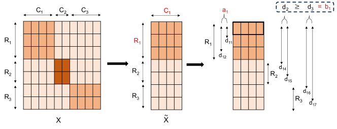
Figure 1: Illustrative example of when both shared rows and columns (in certain pairings) is desirable. Here the same individuals are represented in the rows, but not columns, across $X^{(1)}$, $X^{(3)}$ and $X^{(4)}$. Columns are shared between $X^{(1)}$ and $X^{(2)}$.

ResNMTF addresses these limitations as it can be applied with any combination of restrictions between views, allowing shared row and column clusters to match prior knowledge, and without pre-existing knowledge of the number of biclusters. By regularising the factors towards each other across views ResNMTF avoids issues with noisy views skewing results caused by the use of consensus or shared matrices.

3 Bisilhouette Score

Assessing the obtained biclusters and finding the optimal number of biclusters is an inherited clustering problem. The additional structural complexity of biclusters exacerbates this issue. Existing literature lacks a bicluster specific approach that considers the factors usually deemed necessary for assessing clusters: compactness and degree of separation. Such measures in addition need to allow for non-exhaustivity and non-exclusivity of biclusters.

Current bicluster literature focuses on extrinsic measures that use external information to assess the quality of biclusters [14] or coherence measures [23] that check how closely a bicluster adheres to a specific structure (e.g. constant, coherent). These latter intrinsic measures generally consider biclusters in isolation and ignore any relationships between them. The exception is the Relevance Index (RI) proposed by Yip et al. [24] which considers differences in local and global variation along the columns belonging to a bicluster. However this measure does not penalise for the presence of redundant columns, meaning the presence of irrelevant columns in a bicluster is not necessarily penalised.

Biclusters are often evaluated as two separate sets of clusters (row and column clusters) via standard clustering measures, this risks two issues. Firstly, promising scores can be returned when the rows of a cluster are successfully identified but associated columns are incorrectly or poorly identified (including incorrect matching between row and column clusters if method appropriate). Secondly, a poor score may be returned to a correctly identified bicluster if the bicluster columns are a small portion of the overall matrix. A marked difference across the rows over these columns may be obscured when all columns are considered. The literature lacks a bicluster specific intrinsic measure, a gap that we fill with our bisilhouette score proposal. The proposed measure has the following desirable properties: works for general unsupervised settings, works in the presence of overlapping and/or non-exhaustive biclusters, as well as incorporating both the structure of the bicluster and how it relates to the rest of the data.

The proposed bisilhouette score is based on the popular intrinsic clustering measure, the silhouette score [15] that takes into account compactness and separation of clusters as well as allowing for overlap and non-membership. The silhouette score considers the average distance (typically Euclidean) between an element and others belonging to the same cluster as well as the average distance to the nearest cluster. More specifically, for element $i$ in cluster $k$ the average distance to the other elements in the same cluster is given by $a_{i}=(|R_{k}|-1)^{-1}\sum_{l\in R_{k}}d_{il}$, where $d_{jl}$ be the Euclidean distance between row $j$ and row $l$ of a matrix. The average distance to the elements in the next closest cluster is calculated via $b_{i}=\underset{j\in 1:K,j\neq k}{\text{min}}|R_{j}|^{-1}\sum_{l\in R_{j}}d_{il}$. The silhouette coefficient $s_{i}$ for element $i$ is defined by $s_{i}=(b_{i}-a_{i})/\operatorname{max}(b_{i},a_{i})$. A score for each cluster is returned by averaging over the silhouette coefficients corresponding to the elements in the cluster. These are further averaged to give an overall score for the clustering as in equation:

$$S=\frac{1}{K}\sum_{k=1}^{K}\frac{1}{n_{k}}\sum_{i\in R_{k}}s_{i}$$ (1)

3.1 Bicluster extension

To extend the silhouette score to the bicluster case, the silhouette coefficients are calculated for each row in a given bicluster, based only on the columns corresponding to that bicluster. The score for bicluster $k$ ($B_{k}$) is obtained as follows: the data matrix $X$ is subsetted by the columns belonging to $C_{k}$, $\tilde{X}=X_{.,C_{k}}$. Treating ${R_{j}}$ as the clusters, the silhouette coefficients for the elements of $R_{k}$ on $\tilde{X}$ are calculated. Averaging over the coefficients, $B_{k}$ is found as illustrated in Figure 2.

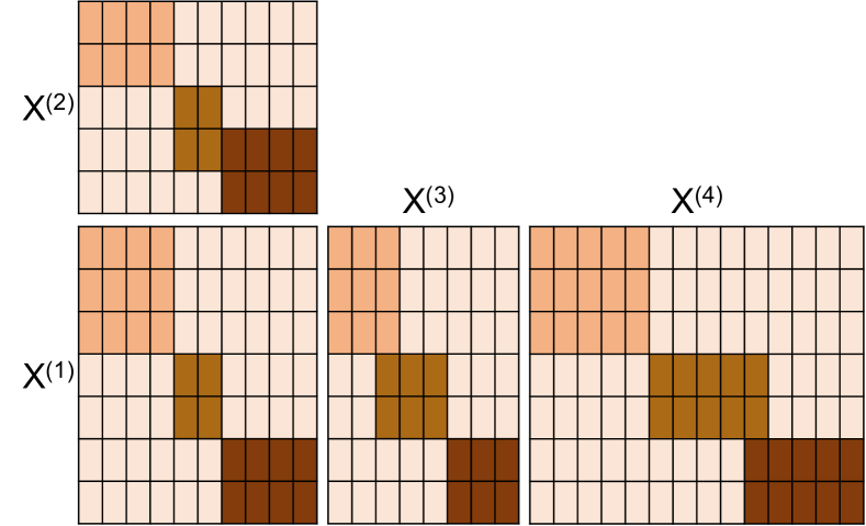
Figure 2: Schematic for the calculation of the bisilhouette score. Matrix $X$ is subsetted by considering the columns belonging to the first bicluster ($C_{1}$), forming $\tilde{X}$. The silhouette score on $\tilde{X}$ is calculated for the rows belonging to the first bicluster ($R_{1}$). These values are averaged to give a score for $(R_{1},C_{1})$.

As with the silhouette score, $B_{k}$ takes values in $[-1,1]$ with a higher score indicating a more compact and well separated bicluster. A value of 1 is obtained if the columns are constant within the bicluster. Care should be taken as this can be achieved when the columns are constant across all rows, not just those belonging to the bicluster. This issue is prevented by removing features with zero/very low variance. An overall bisilhouette score $B$ for the biclustering $\{(R_{k},C_{k})\}_{1:K}$ is given by calculating the mean over the non-zero $B_{k}$ and subtracting twice their standard deviation. The subtraction of the standard deviation accounts for large variability in the quality of biclusters, indicating a poor overall biclustering. A score of zero is assumed to correspond to an empty bicluster - a non-empty bicluster with score exactly zero is very unlikely for data with any signal present. The above assumes all $R_{k}$ and $C_{k}$ are non-empty and there are at least three unique sets amongst the row clusters. The case where there are fewer than three unique row clusters is treated separately in A.1. With these edge cases considered, the bisilhouette score can be calculated for any number of biclusters, allowing for comparison between any two sets of biclustering results. This is in contrast to the silhouette score which is only defined for two or more clusters.

4 Restricted Non-negative Matrix Tri-Factorisation

This section introduces the novel biclustering approach, ResNMTF, that is based on non-negative matrix tri-factorisation. The aim of the proposed approach is to identify biclusters amongst the integrated data-views whilst allowing for any non-exhaustivity and/or non-exclusivity to be present. The approach is combined with a stability analysis technique that checks the stability of the selected biclusters.

4.1 Non-negative tri-matrix factorisation and Extensions

The standard NMTF approach factorises the non-negative design matrix $X\in\mathbb{R}^{N\times p}$ into a product of three matrices (as opposed to two factors in NMF), such that $X\approx FSG^{T}$ where $F\in\mathbb{R}^{N\times K},S\in\mathbb{R}^{K\times L}$ and $G\in\mathbb{R}^{p\times L}$. Here $K$ denotes the number of row clusters and $L$ denotes the number of column clusters, with $K=L$ often chosen.

Multi-view NMTF approaches seek matrix factorisations for each view $v\in{1:n_{v}}$, $X^{(v)}\approx F^{(v)}S^{(v)}(G^{(v)})^{T}$, with appropriate dimensions implied for all matrices. Like in multi-view NMF methods (which seek factorisations $X^{(v)}\approx F^{(v)}(W^{(v)})^{T}$), commonality across the views can be implemented via different means. Akata et al. [25] implement a shared $F$ matrix, setting $F=F^{(v)}$ for all $v$. Others regularise the matrices corresponding to row cluster assignments for each view ($F^{(v)}$) towards a single consensus matrix $F^{*}$ [26]. CoNMF proposed by He et al. [27] regularises factors towards each other via penalty terms such as $\|F^{(v)}-F^{(w)}\|$. By clustering with individual factors for each view CoNMF aims to alleviate the impact on performance a single poor quality view has [27]. Yang et al. [28] proposed CoNMTF that extends CoNMF to the biclustering case where similarly to other NMTF multi-view methods [20, 29, 28], it is based on relational matrices and is therefore not applicable in a general setting.

ResNMTF, similarly to CoNMTF, extends CoNMF to the biclustering case but in contrast to coNMTF is suitable for application with general multi-view data. The regularisation of factors implemented in ResNMTF tackles a key difficulty associated with multi-view integration methods. As it is not possible to know which are the noisy views and which are the informative ones, a desirable property of a proposed method is its ability to prevent noisy views from corrupting the signal of the informative ones. By regularising the factors towards each other across views, the relationships between views are accounted for, whilst avoiding issues with noisy views skewing results caused by the use of consensus or shared matrices [26].

A multi-view NMTF approach to multi-view biclustering inherits several problems from both NMF and NMTF. Firstly, as with NMF, restrictions on matrix factors are needed to ensure uniqueness of solution. Additional constraints are required moving from NMF to NMTF to prevent reformulation as an NMF solution, for example with the two factors $F$ and $SG$. Such constraints include orthogonal constraints on both $F$ and $G$ [5]. As with all methods involving update-based optimisation procedures, like NMF, initialisation procedures are required - this motivates our proposal of an initialisation procedure suitable for NMTF based methods in Section 4.4. Lastly, NMTF requires pre-specification of the number of biclusters ($K$). When prior information is available regarding the true number of biclusters, this value of $K$ can be used to obtain the result. However, in most unsupervised learning cases the optimal value of $K$, $\hat{K}$, is unknown. Within ResNMTF various possible values of $K$ are considered and the bisilhouette score determines the optimal value. This pre-specification of $K$ does not allow for all possible scenarios. Suppose a particular view doesn’t contain any biclusters, simple NMTF based approaches will still return biclusters for this view. In light of this, ResNMTF (via a resampling approach) assesses each bicluster and removes those that are deemed to represent noise rather than signal. This removal, alongside the stability analysis procedure, ensures only stable biclusters representing true signal are returned by ResNMTF.

The section starts with a presentation of the optimisation problem with the set of update steps taken as well as the proposal of the initialisation technique. A discussion of how biclusters are assigned amongst the integrated data-views is presented. Next, the steps taken for removing spurious biclusters and checking the stability of the selected ones are presented. The section ends with the implementation of the approach.

4.2 Objective

By assuming a known $K$, $K\geq 3$, the aim of Restricted Non-negative Matrix Tri-Factorisation is to solve the optimisation problem given:

$$\hskip 56.9055pt\min_{F^{(v)},S^{(v)},G^{(v)}}\left(\sum_{v=1}^{n_{v}}\left\|X^{(v)}-F^{(v)}S^{(v)}\left(G^{(v)}\right)^{T}\right\|^{2}\right.\hskip 56.9055pt$$ (2)

$$\left.+\sum_{w=v+1}^{n_{v}}\sum_{v=1}^{n_{v}-1}\left(\phi_{vw}\left\|F^{(v)}-F^{(w)}\right\|^{2}+\xi_{vw}\left\|S^{(v)}-S^{(w)}\right\|^{2}+\psi_{vw}\left\|G^{(v)}-G^{(w)}\right\|^{2}\right)\right)$$

such that for all $v$ in $1:n_{v}$

• $||F^{(v)}_{.,k}||,||G^{(v)}_{.,k}||=1,\quad\forall k=1,2,\cdots,K$

• $F^{(v)},S^{(v)},G^{(v)}\geq 0$

where $\Phi=(\phi)_{vw}$, $\Xi=(\xi)_{vw}$, $\Psi=(\psi)_{vw}$ are upper triangular non-negative matrices. $\phi_{vw},\xi_{vw},\psi_{vw}$ are tuning parameters allowing for different restrictions. Different combinations of tuning parameters enforce different combinations of restrictions. For example, non-zero $\phi_{12}$ means views one and two share common row clusters, therefore $F^{(1)}$ and $F^{(2)}$ are forced towards each other. After minimising the objective function defined in Eq.(2), factors $F^{(v)},S^{(v)}$ and $G^{(v)}$ for each view $X^{(v)}$ are obtained. The factors for view $v$ determine biclusters $BC_{K}^{(v)}$, giving the a multi-view biclustering result, $BC_{K}$.

By including the regularisation of both $S^{(v)}$ and $G^{(v)}$ matrices in the objective function allows for different biclustering scenarios. Such scenarios include common column clustering across views rather than or in addition, to across views.

4.3 Update steps

The objective function of NMTF is non-convex and minimising it has been shown to be an NP-hard problem [30]. However, by fixing all matrices except one, the problem becomes convex allowing it to converge towards a local stationary point [5, 31]. Following the work by Long et al. [32] and He et al. [27], which are themselves based on the algorithm by Lee and Seung [33], a local solution to this problem is found via multiplicative update rules. The update rules move the variables along the gradient direction. This involves initialising factors $F^{(v)},S^{(v)}$ and $G^{(v)}$ for each view and iteratively applying multiplicative updates to each matrix, until some predetermined notion of convergence is met. As our objective function requires normalisation and non-negativity constraints to be met, Lagrangian multipliers $\lambda_{k}^{(v)}$ and $\mu_{k}^{(v)}$ are added to the objective function that are also iteratively updated. The update steps are as follows:

$$F^{(v)} \leftarrow F^{(v)}\odot\frac{X^{(v)}G^{(v)}\left(S^{(v)}\right)^{T}+\sum_{u=1}^{n_{v}}\phi_{uv}F^{(u)}}{F^{(v)}S^{(v)}\left(G^{(v)}\right)^{T}G^{(v)}\left(S^{(v)}\right)^{T}+\left(\sum_{u=1}^{n_{v}}\phi_{uv}\right)F^{(v)}+\frac{1}{2}\boldsymbol{1}\Lambda^{(v)}}$$

$$S^{(v)} \leftarrow S^{(v)}\odot\frac{(F^{(v)})^{T}X^{(v)}G^{(v)}+\sum_{u=1}^{n_{v}}\xi_{uv}S^{(u)}}{\left(F^{(v)}\right)^{T}F^{(v)}S^{(v)}\left(G^{(v)}\right)^{T}G^{(v)}+\left(\sum_{u=1}^{n_{v}}\xi_{uv}\right)S^{(v)}}$$

$$G^{(v)} \leftarrow G^{(v)}\odot\frac{(X^{(v)})^{T}F^{(v)}S^{(v)}+\sum_{u=1}^{n_{v}}\psi_{uv}G^{(u)}}{G^{(v)}\left(S^{(v)}\right)^{T}\left(F^{(v)}\right)^{T}F^{(v)}S^{(v)}+\left(\sum_{u=1}^{n_{v}}\psi_{uv}\right)G^{(v)}+\frac{1}{2}\boldsymbol{1}M^{(v)})}$$

$$\Lambda^{(v)} \leftarrow\Lambda^{(v)}\odot(\boldsymbol{1}^{T}F^{(v)})$$

$$M^{(v)} \leftarrow M^{(v)}\odot(\boldsymbol{1}^{T}G^{(v)})$$

where $\Lambda^{(v)}=(\lambda_{1}^{(v)},\dots,\lambda_{K}^{(v)})$ and $M^{(v)}=(\mu_{1}^{(v)},\dots,\mu_{K}^{(v)})$. A full derivation of the update steps can be found in A.2.

For iteration $i$, the error is given by:

$$E_{i}=\frac{1}{n_{v}}\sum_{v=1}^{n_{v}}E_{v}\ \text{where}\ E_{v}=\|X^{(v)}-F^{(v)}S^{(v)}\left(G^{(v)}\right)^{T}\|^{2}/\|X^{(v)}\|^{2}$$ (3)

A convergence based stopping criteria with a tolerance of $e^{-6}$ between successive errors is implemented as suggested in Čopar et al. [34].

4.4 Initialisation

As non-convexity only guarantees a local solution to NMTF, the initialisation of factors is extremely important in the success of the method. The proposed initialisation strategy builds upon the work of Boutsidis and Gallopoulos [35] and Riddle-Workman et al. [20] for NMTF based methods and is applied to each view separately. The proposed initialisation is suitable for general matrices and provides a different initialisation for each view in contrast to the work of Riddle-Workman et al. [20].

$F$ and $G$ are initialised as:

$$F \leftarrow(\text{abs}(\boldsymbol{u}_{1}),\dots,\text{abs}(\boldsymbol{u}_{K}))\text{diag}\left(\{1/||\boldsymbol{u}_{k}||\}_{1:K}\right)$$

$$G \leftarrow(\text{abs}(\boldsymbol{v}_{1}),\dots,\text{abs}(\boldsymbol{v}_{K}))\text{diag}\left(\{1/||\boldsymbol{v}_{k}||\}_{1:K}\right)$$

where $\sigma_{k}$ are non-negative values that correspond to the singular values of $X$ in decreasing order, $\boldsymbol{u}_{k}$ and $\boldsymbol{v}_{k}$ are the corresponding left and right singular vectors respectively. Both matrices have been normalised to that they satisfy the necessary normalisation constraints presented earlier.

$S$ is initialised as the sum of the diagonal matrix of the first $K$ singular values plus a $K\times K$ matrix of noise with entries from $N(0,\sigma_{N}^{2})$. The multiplicative nature of the updates require the addition of positive noise to allow for non-zero off-diagonal entries in $S$ and $\sigma_{N}$ denotes our belief that the biclusters are distinct. $S$ then absorbs the normalisation factors from $F$ and $G$ giving:

$$S \leftarrow\text{diag}\left(\{||\boldsymbol{u}_{k})||\}_{1:K}\right)(\text{diag}(\{\sigma_{k}\}_{1:K})+\text{abs}(N))\text{diag}\left(\{||\boldsymbol{v}_{k}||\}_{1:K}\right)$$ (4)

The initial values of multipliers $\Lambda$ and $M$ are $\Lambda=M=\boldsymbol{1}^{T}$.

4.5 Bicluster assignment

The factors obtained from the optimisation outlined in Eq. 2 are used for deriving the obtained biclusters. As $F_{ik}$ represents the association of row $i$ to $\tilde{R}_{k}$ and column normalisation requires $||F_{.k}||=1$, the following relation determines row clusters assignment:

$$\tilde{R}_{k}=\left\{i:F_{ik}>\frac{1}{n_{r}}\right\}$$

If $X$ is pure noise, all rows would be equally weakly associated to a given row cluster. Therefore row $i$ is assigned to $\tilde{R}_{k}$ if it is more strongly associated to the cluster than expected if the data was purely noise.

Similarly, $G_{ik}$ represents the association of column $j$ to column cluster $k$ ($\tilde{C}_{k}$) and so column clustering is determined via:

$$\tilde{C}_{k}=\left\{i:G_{ik}>\frac{1}{n_{c}}\right\}$$

As all row and column clusters are treated independently, this assignment technique allows for non-exhaustive and non-exclusive biclusterings. Additionally, this cluster assignment allows for complete overlap in either dimension. Finally, $BC_{k}$ is defined by matching the row cluster $\tilde{R}_{l}$ to $\tilde{C}_{k}$ via $l=\operatorname{argmax}_{j}S_{jk}$.

4.6 Removal of spurious biclusters

Following the assignment of biclusters, the results are checked to ensure the biclusters are a true signal. Spurious biclusters are identified and removed from the biclustering. Biclusters are classified as spurious ones if they do not differ from what is expected from noise. The following re-sampling procedure is applied for identifying the spurious biclusters. For resampling $m$, the entries of the original data matrix ${X^{(v)}}_{1:n_{v}}$ are shuffled creating a pure noise data matrix, $\hat{X}^{(v)}_{m,1:n_{v}}$. The objective function in Eq. 2 is solved for the shuffled data-views and the factors $\hat{F}^{(v)}_{m,1:n_{v}}$ are obtained. For each $v$, $\hat{X}^{(v)}_{m}$ is pure noise and all rows are equally weakly associated to each bicluster. Therefore each entry of $\hat{F}^{(v)}_{m}$ is independent and identically distributed. These column vectors will be differently distributed to those from the original factors corresponding to true biclusters (as illustrated in Figure 3). The Jensen Shannon divergence (JSD) [36] (see A.3.1 for details) is used to test the similarity between column vectors obtained from the true data vector and the noisy one. When the distribution of the column vector does not differ significantly from that obtained from the noisy data, the bicluster is deemed false and removed. For every $v$, each column of $F^{(v)}$ is considered independently, allowing for any particular bicluster to be removed. Consider the multi-omics example where biclusters correspond to disease subtypes; a particular subtype may have distinguishing features in a certain omic. By examining columns of $F^{(v)}$ separately allows for this scenario. The method is specified in detail in A.3 with pseudocode provided in Algorithm 2.

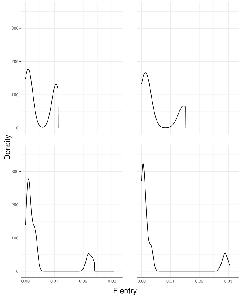
(a) Original

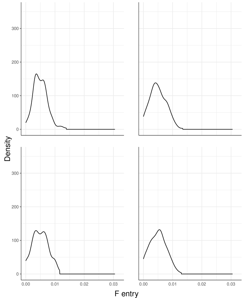
(b) Shuffled

Figure 3: Plot of the estimated density of each column of $F^{(1)}$ obtained from solving Eq. 2 for (a) original and (b) reshuffled synthetic data. The synthetic data was generated using the process outlined in Section 5.1, with 4 biclusters across 2 views of dimension $200\times 100$ and $200\times 250$.

4.7 Determining the number of biclusters

Biclustering is often applied in unsupervised settings and hence the number of biclusters present is unknown. In order to determine the optimal number of biclusters $\hat{K}$, ResNMTF considers a range of possible values $K\in(K_{min},K_{end})$. The procedure for removal of spurious biclusters is performed for each value of $K$, returning a biclustering $BC_{K}$. The bisilhouette score for each $BC_{K}$ is calculated ($B_{K}$) and used to select between biclusterings. When the bisilhouette score is maximised at either limit of $k$ ($\hat{K}=K_{min}$ or $K_{end}$), the current implementation of ResNMTF extends the range of values considered until this is not the case.

4.8 Stability analysis

von Luxburg [13] define the instability of a clustering algorithm as the expected distance between two clusterings produced from two different samples of the same size. The same principle applies in biclustering. Even after removing spurious biclusters, unstable biclusters may stay. Motivated by the general algorithm for calculating stability score in von Luxburg [13] as well as the work in Duong-Trung et al. [37], a strategy is implemented for assessing the biclusters through a sub-sampling technique. After applying the sub-sampling method introduced below, the results are compared to the results of the original data, and any biclusters with consistently low similarity to the resampled results are deemed unstable and removed.

The re-sampling procedure is described here. The $m^{th}$ resampled dataset is produced by randomly sub-setting matrix $X^{(v)}$, producing submatrix $\tilde{X}_{m}^{(v)}$ consisting of $\lfloor\alpha n_{r}^{(v)}\rfloor$ rows and $\lfloor\alpha n_{c}^{(v)}\rfloor$ columns. Here $\alpha$ is the sample rate (default value 0.9) and denotes the portion of the original data in the resampled dataset. If shared row and/or column cluster restrictions are imposed, this is imposed here with the resampling consistent across the relevant dimension and views. The same subsampling is applied to the original biclustering producing $\text{BC}^{(v)}_{m}$, allowing for meaningful comparisons. ResNMTF is performed on $\{\tilde{X}_{m}^{(v)}\}_{1:n_{v}}$ with the number of biclusters fixed and equal to $\hat{K}$, producing biclustering $\tilde{\text{BC}}_{m}$. Since a ‘ground truth’ labelling is available (the original biclustering BC), the extrinsic measure relevance (defined in B.1) is used to compare the results achieved from the subsample with those from the original data to produce a similarity score for each bicluster $l$ in each view, $\text{Rel}^{(v)}_{lm}\left(\text{BC}^{(v)}_{m},\tilde{\text{BC}}_{m}^{(v)}\right)$. This is repeated $n_{s}$ times and the mean score across repetitions ($\bar{\text{Rel}}^{(v)}_{l}$) is calculated and if $\bar{\text{Rel}}^{(v)}_{l}\leq\omega$ for some threshold $\omega$, bicluster $l$ in view $v$ is deemed unstable and the update $R^{(v)}_{l}=C^{(v)}_{l}=\emptyset$ is performed. The number of repetitions controls the number of subsampled datasets used to estimate the average, with $n_{s}=5$ used as default. The threshold $\omega$ controls the balance between recovering all biclusters to some degree and ensuring those biclusters returned are stable. It is a hyperparameter to be tuned and the choice depends on the application setting and the desired properties of the results.

4.9 Implementation

Pseudocode describing the implementation of stability analysis within ResNMTF is provided in Algorithm 3 and the application of ResNMTF is summarised in Algorithm 1. The code required to implement ResNMTF and the bisilhouette score can be found at https://github.com/eso28599/resNMTF.

Algorithm 1 Implementation of ResNMTF

1:Input: multi-view data $\{X^{(v)}\}_{1:n_{v}}$, possible range of number of biclusters $(K_{\text{min}},K_{\text{end}})$ (default $(3,8)$), restriction hyperparameters $\Phi,\Psi,\Xi\in\mathbb{R}^{n_{v}\times n_{v}}$ (default $\mathbf{0}$), inputs for Algorithm 2 and Algorithm 3

2:Output: biclustering $BC_{\hat{K}}=\{\{(R^{(v)}_{i},C^{(v)}_{i})\}_{i\in 1:\hat{K}}\}_{v\in 1:n_{v}}$

3:Procedure:

4:$(K,\hat{K})\leftarrow(K_{\text{min}},K_{\text{end}})$

5:while $k\leq k_{\text{end}}$ or $\hat{K}=k_{\text{end}}$ do

6:  Initialise $\{F^{(v)},S^{(v)},G^{(v)}\}_{1:n_{v}}$ for $K$ biclusters

7:  repeat

8:   Update $\{(F^{(v)},S^{(v)},G^{(v)})\}_{1:n_{v}}$

9:  until Eq. 3 converges

10:  Extract biclusters, $BC_{K}$

11:  Remove spurious biclusters using Algorithm 2

12:  Calculate the bisilhouette score, $B_{K}$

13:  $\hat{K}\leftarrow\underset{j\in\{K_{\text{start}},\dots,K\}}{\text{argmax}}B_{j}$

14:  $K\leftarrow K+1$

15:end while

16:Perform stability selection on $BC_{\hat{K}}$ using Algorithm 3

5 Numerical Experiments

This section demonstrates the performance of ResNMTF and the efficacy of the bisilhouette score as an intrinsic measure on both synthetic and real datasets with different characteristics. ResNMTF is compared with the unrestricted NMTF, implemented via $\Phi=\Psi=\Xi=0$. Unrestricted NMTF is applied in a similar fashion as ResNMTF following the steps described in Section 4. In addition, ResNMTF is compared with the competing methods iSSVD and GFA, the implementation of which is presented in B.5.

The performance of the multi-view biclustering approaches is assessed by calculating both extrinsic and intrinsic measures. The Jaccard [38] based measures relevance and F-score (defined for biclusters in B.1) are used to evaluate the quality of returned biclusters, comparing the reported biclusters with the underlying true biclusters. Our proposed intrinsic measure, the bisilhouette score (abbreviated as BiS; described in Section 3) is also reported. Throughout the conducted experiments, these scores are calculated for each view individually and averaged. For both measures a score closer to 1 indicates better performance.

The section is structured as follows. A description of the synthetic and real data analysed is provided. Subsequently a discussion on how the hyper-parameters, $\Phi,\Psi$ and $\omega$, of ResNMTF are tuned is presented. The section ends with a presentation of the findings from the conducted analyses. The conducted analyses are used to address the following key questions:

1. Is the bisilhouette score a powerful measure to identify the correct number of biclusters?

2. How does the bisilhouette score compares with other intrinsic and extrinsic measures for evaluating biclusters?

3. Is ResNMTF able to correctly identify the biclusters of the data?

4. How does ResNMTF compare with other biclustering approaches, including unrestricted NMTF, iSSVD and GFA?

5.1 Data

Synthetic data were created where the true structure is known to assess the performance of ResNMTF under different scenarios including number of views, biclusters or individuals, as well as noise levels.

For each view $v$, the data matrix $X^{(v)}$ is generated as the sum of the absolute values of a signal matrix, $B^{(v)}$, and a noise matrix, $\mathcal{E}^{(v)}$. The absolute values are used to ensure non-negativity of the data. The entries of the noise matrix $\mathcal{E}^{(v)}$ are drawn from a $N(0,\sigma^{2})$ distribution, with the $\sigma$ parameter controlling the level of noise in the data. In the conducted experiments the default value of $\sigma$ was taken equal to 5, and in the experiments where the effect of noise was investigated the value of $\sigma$ was varied between 1 to 100.

Each bicluster is represented by a block matrix, $B_{k}^{(v)}$, along the diagonal of $B^{(v)}$ i.e. $B^{(v)}=\text{bdiag}(\{B_{k}^{(v)}\}_{1:K})$, as illustrated in Figure 4. $B_{k}^{(v)}$ has $r_{k}$ rows and $c_{k}$ columns. The entries of these blocks are samples from a Normal distribution with mean $\mu$ and variance $\sigma_{B}^{2}$ ($N(\mu,\sigma_{B}^{2})$), where in the conducted experiments the parameters were set up as 5 and 1 respectively. As $\sigma_{B}$ is independent of $k$ and $v$, the within-bicluster variation is constant both across a view and between all views. The exhaustive exclusive biclusters are generated in such a way so that the row clusters are shared across the views but separate column clusters exist. For a given number of rows/columns and number of biclusters, the dimensions ($(r_{1},\dots,r_{K})/(c_{1},\dots,c_{K})$) were fixed as follows for consistency. Biclusters are ordered in decreasing size, with an initial ratio of 4:3 for $K=2$. As the number of biclusters increases by one, the part corresponding to the current largest bicluster splits in two, with $2r+1$ being split into $r+1$ and $r$. Any remainders from scaling the ratios are added to the first of the smallest biclusters. For example, if $K=5$, $n_{v}=2$, and $n_{r}=200$, the row clusters are $(55,55,31,27,27)$ (as illustrated in Figure 4). The number of individuals is fixed in most experiments at $n=200$, except when this is the factor being investigated in which case it varies from 50 to 1000. Similarly, most experiments are conducted on three views with 100, 50 and 250 features in each view, with the exception of the study on increasing number of views when all views have 150 features. As a final step, the rows and columns of $X^{(v)}$ are shuffled to more accurately represent expected data. The same row shuffling is applied across all views whilst column shuffling is done independently. Amendments to this process to produce overlapping and/or non-exhaustive biclusters are outlined in B.2.

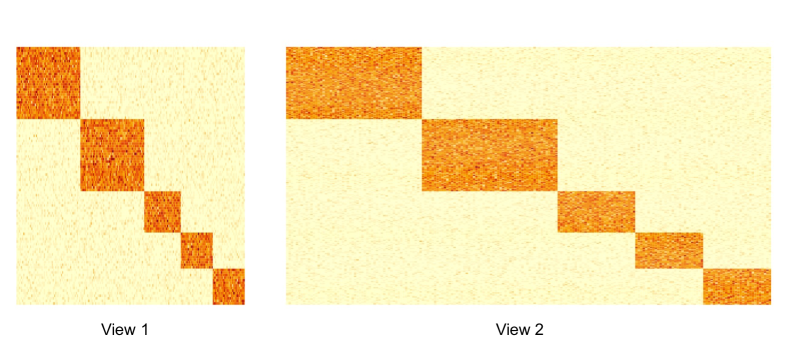
Figure 4: Synthetic data example. Column cluster dimensions are $(27,27,15,13,13)$ in view 1 and $(69,69,39,34,34)$ in view 2.

The following real multi-view datasets, summarised in Table 1, are also analysed. The pre-processing steps applied to the datasets are outlined in B.3.

• 3Sources is a popular dataset that includes articles on the same topics reported by three different news outlets (corresponding to the three separate views); the Guardian, BBC, and Reuters. Each view is a document-term matrix presenting 169 articles (documents) and the counts of various words (terms) across the articles. There are 3393, 3553 and 2998 terms in each of the views respectively. Each article was manually labelled by the source as one or more of six categories; business, entertainment, health, politics, sport or tech.

• BBCSport contains 169 articles which have been split into two parts (corresponding to two views). Each article has been labelled in one of the five categories: athletics, cricket, football, rugby, tennis. The two views contain 3173 and 3195 terms, respectively.

• A459 is a single cell multi-omic dataset obtained from a kidney tissue of a mouse [39]. The subtypes represent differential treatment time of the cells of either 0, 1 or 3 hours. Transcriptomic (scRNA-seq) and epigenomic (scATAC-seq) data are obtained on the 2641 cells, with the views containing 1176 and 1147 genes respectively.

Datasets	Clusters	View	Samples	Features
3Sources	6	3	169	$(3393,3553,2998)$
BBCSport	5	2	544	$(3173,3195)$
A549	3	2	2641	$(1176,1147)$

Table 1: Summary of the real datasets used including the number of true row clusters present, the number of views in each dataset, the number of samples (which is equal for each view) and the number of features in each view.

All datasets are sparse with 3Sources and BBCSport containing non-zeros in less than 5% of entries, and A549 in less than 25%. Euclidean distance is not typically used for sparse data with the Manhattan or cosine distances preferred. Whilst for A549 the performance with different distances is comparable, for the two datasets with over 95% sparsity an improvement is observed with the cosine distance (Table 3). In the subsequent analyses the bisilhouette score is therefore implemented with the cosine distance for the 3Sources and BBCSport datasets.

5.2 Hyperparameter tuning

This section discusses the hyperparameter values and tuning implemented in the application of ResNMTF to both the synthetic and real data. Two alternative approaches for the two sets of data were implemented.

For all experiments concerning synthetic data, the biclusters are constructed to share common row clusters across rows and so restrictions between views are implemented via non-zero $\Phi$ with $\Psi=\Xi=0$. Each pairwise restriction has the same weighting i.e. all $\phi_{vw}=\phi$ for some constant $\phi$. By varying $\phi$ across different scenarios, a suitable value of $\phi=200$ for the synthetic data is found (see B.4 for details). Stability analysis is performed with $\omega=0.4$ (see Section 4.8 for the description of this hyperparameter). The value of $\omega$ applied on the synthetic datasets was selected based off preliminary investigations, however tuning of the stability analysis hyperparameter is investigated further on the real datasets.

In all the real datasets the samples are the shared dimension. The decision whether or not to transpose the views does affect results - for example, in the selection of the number of biclusters the bisilhouette score calculates the silhouette score of row clusters over columns corresponding to a bicluster. For 3Sources and BBCSport, matching terms to documents improves performance and so both datasets are transposed with restrictions enforced via non-zero $\Psi$. In contrast, for the single-cell A549 dataset, performance is not improved by transposing and restriction is enforced via non-zero $\Phi$ for A549. As with the analysis of the synthetic data, restrictions are assumed to be equal between views with $\psi_{i,j}=\psi$ ($\phi_{i,j}=\phi$) for non-zero $\psi_{i,j}$ ($\phi_{i,j}$).

In the analysis of the real datasets, three strategies were considered for the tuning of the restriction and stability analysis hyperparameters. Restriction hyperparameters are optimised first, followed by the stability threshold. The first strategy is suitable for an unsupervised setting and uses the bisilhouette score to select the optimal hyperparameters - this is denoted ResNMTF (BiS/BiS). Secondly, the restriction hyperparameter is optimised via the bisilhouette score but $\omega$ is optimised using the F-score and is denoted by ResNMTF (BiS/F-score). Through this strategy, the ability of the bisilhouette score to correctly determine the optimal hyperparameters in the stability analysis and the restriction case, is disentangled. The final strategy considers the supervised setting where true labels are available. Here both hyperparameters are optimised via the F-score and the approach is denoted by ResNMTF (F-score/F-score). All implemented strategies do not require any user input, but ResNMTF (BiS/BiS) is the only strategy applicable in an unsupervised setting. As all methods (including GFA and iSSVD) involve some degree of random initialisations the methods are applied on the real datasets with 5 different seeds. The F-score is used to select the best result between the repeats for NMTF, GFA and iSSVD, whereas for ResNMTF applications the measure used to optimise $\omega$ is used to select between the 5 repetitions (i.e. the F-score for ResNMTF (BiS/F-score). As for most real datasets, only information about clusters present, and not the features that drive those clusters, is known. Recovery, relevance and the F-score for the real datasets are therefore calculated based on the row clusters alone.

5.3 Results

5.3.1 ResNMTF performance

ResNMTF and NMTF are found to have similar performance and/or similar trends in their performance, with the former outperforming the latter in most cases (Figure 5). Both approaches consistently outperfom both GFA and iSSVD. The performance of (Res)NMTF drops as the number of biclusters, and as expected, the level of noise, increases. Surprisingly, the performance of the methods is not found to improve as the number of individuals increases. NMTF outperforms ResNMTF when the number of views are increased and this is also seen when we consider 4 instead of 5 biclusters (Figure 15). One possible explanation for this is that the value of $\phi$ applied on the synthetic data depends strongly on the number of views.

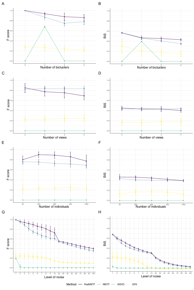
Figure 5: F-score (left column) and BiS (right column) for different methods: base scenario of 200 rows, 3 views (100, 50 and 250 columns), 5 biclusters and $\sigma=5$. The number of (A-B) biclusters (C-D) views (150 columns each) (E-F) individuals or (G-H) the level of noise are varied. The average score across 100 repetitions is reported with $\pm$ standard deviation error bars presented.

GFA’s performance is largely invariant to all factors investigated apart from noise whilst iSSVD is mostly unable to detect biclusters when applied with the default parameter values. This is despite extensive effort to tune hyperparameters (Figures 10 and 11). Additionally, we investigated at what level of signal ($\mu$) iSSVD is able to detect biclusters (Figure 12), as well as applying all the methods to data generated as described in Zhang et al. [16] (Figure 18). See B.5.2 for details.

The presence (and indeed the rate) of overlapping biclusters has no discernable effect on the performance of ResNMTF, NMTF and GFA (Figure 17). Whilst the performance of ResNMTF/NMTF does fall as the rate of non-exhaustivity increases, both methods remain superior to GFA and iSSVD. The performance of iSSVD in contrast is found to be improved in the presence of overlapping and/or non-exhaustive biclusters.

ResNMTF applied on 3Sources or A549 using any of the tuning strategies outperforms all other methods (Table 2). For BBCSport, ResNMTF optimised via F-score outperforms all other methods. The bisilhouette score appears less able to the stability analysis parameter in this setting. This may be caused by the sparsity of the dataset and the lack of suitability of the cosine distance in tuning the stability analysis parameter. With no stability analysis performed and cosine distance used within the method, ResNMTF achieves an F-score of $0.5975$ (Table 3). In all cases, integrating the multiple data-views via a non-zero restriction hyperparameter improves the biclustering performance of ResNMTF. Figure 6(a) illustrates that stability analysis perform as desired on the 3Sources dataset with the relevance of remaining biclusters increasing as the threshold increases.

Method	3Sources	BBCSport	A549
ResNMTF (BiS/BiS)	0.4720	0.2582	0.4216
ResNMTF (BiS/F)	0.5223	0.5411	0.4895
ResNMTF (F/F)	0.5166	0.6247	0.5029
NMTF	0.4668	0.5889	0.3884
GFA	0.4418	0.3303	0.3705
iSSVD	0.2828	0.5090	0.0845

Table 2: F-score of ResNMTF and competing methods on real datasets. Optimisation measure of restriction and stability hyperparameters denoted in brackets e.g. (BiS/F) means $\phi/\psi$ is selected by maximising the bisilhouette score and $\omega$ is selected by maximising F-score. Best results in bold.

5.3.2 Bisilhouette score performance

Visually, the bisilhouette score demonstrates very similar trends to that of the F-score. This is confirmed quantitatively as the bisilhouette score correctly identifies the best performing method in $100\%$ of the scenarios considered in Figure 5, whilst the ranking of methods by F-score and the bisilhouette score have a Pearson correlation of 0.944 (3sf) with disagreements only appearing between the two worst performing methods. This trend is further demonstrated in the remaining results presented in B, most notably whilst tuning hyperparameters on iSSVD (Figures 10 and 11), in the presence of overlapping and non-exhaustive biclusters (Figure 17) and when considering data generated via an alternative process (Figure 18). This demonstrates the use of the bisilhouette score outside of ResNMTF, as a tool for tuning hyperparameters and comparing results in an unsupervised setting.

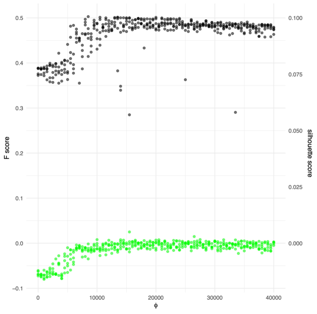
Figure 19: F-score (left y axis, black) and the silhouette score (right y axis, green) against $\phi$ on A549 dataset. The method was applied with each value of $\phi$ for 5 different seeds and all datapoints are shown.

The analysis of the real datasets illustrates the suitability of the bisilhouette score for selecting the hyperparameter values, in particular for the selection of the restriction hyperparameters as previously discussed (Table 2). In particular, we see the bisilhouette score is able accurately select the optimal restriction hyperparameter values for the A549 dataset, and is in agreement with the findings of the analysis using the F-score resulting in a Pearson correlation of 0.867 between the scores (Figure 6(b)). Notably the bisilhouette score demonstrates superior performance in hyperparameter tuning compared with the traditional silhouette score. If the silhouette score is instead used to tune $\phi$ for A549, the correlation between the intrinsic measure and F-score falls to 0.711 (3sf) (Figure 19).

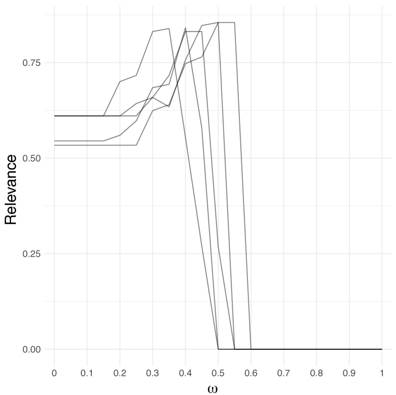
(a) $\omega$ selection

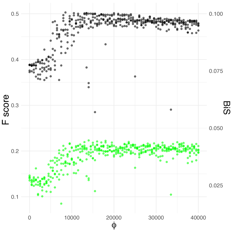
(b) $\phi$ selection

Figure 6: Hyperparameter tuning: (a) relevance against $\omega$ on 3Sources dataset (using $\psi$ optimised by the bisilhouette score) and (b) F-score (left y axis, black) and the bisilhouette score (right y axis, green) against $\phi$ on A549 dataset. In (a), each line corresponds to the results from one of 5 random seeds. In (b) the method was applied with each value of $\phi$ for 5 different seeds and all datapoints are shown.

Similar to the original silhouette score, the bisilhouette score can be used as a visualisation tool to aid in assessing biclusters. Figure 7(a) demonstrates the use of these plots in flagging potentially incorrect biclusters whilst Figure 7(b) highlights how these plots may be used to verify results. Further, the plots may be used to elicit information regarding the biclusters - Figure 7(b) demonstrates that whilst all biclusters appear to have captured some signal, perhaps bicluster 2 represents a more marked differentiation.

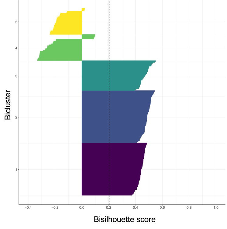
(a) Synthetic data

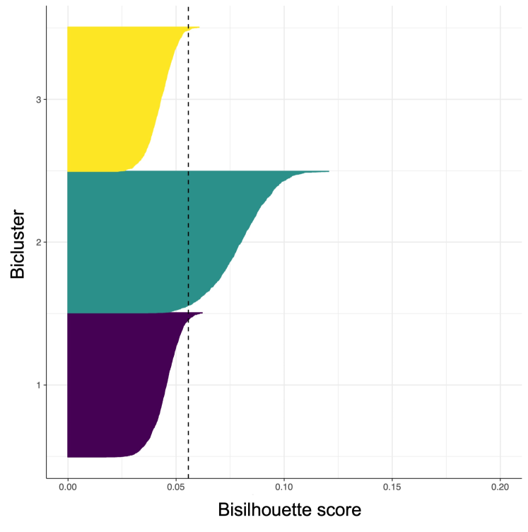
(b) A549

Figure 7: Bisilhouette plots for view one of (a) synthetic data with 3 views and 5 biclusters using the true column clusters and 3 out of 5 of the correct row clusters with the remaining row clusters having been reassigned randomly, and (b) the A549 dataset. The individual bisilhouette coefficients for each of the rows is shown along the x axis, with rows grouped into the assigned biclusters (denoted by different colours). The mean coefficient is represented by the dashed line. Note that the axes ranges are different as the bisilhouette score is not comporable across distinct datasets.

6 Conclusion and discussion

This paper proposes an intrinsic measure for evaluating biclustering solutions, the bisilhouette score. The proposed score is a promising solution for tuning hyperparameters and selecting between biclusterings in an unsupervised setting. The bisilhouette score does appear less adapt at selecting the the stability analysis parameter than the restriction hyperparameter, within ResNMTF. This may be due to the presence of sparsity and a possible lack of suitability of the cosine distance for this task, with the resampling procedure within the stability analysis potentially having a larger effect if greater sparsity is present. However, the promising results warrants further investigation into the use of the bisilhouette in tuning hyperparameters. Similarly to the original silhouette score, it provides visualisations which can aid in the assessment of biclustering quality. These qualities make the bisilhouette score an important tool in the application of biclustering methods in an unsupervised setting. Verma et al. [40] have previously extended the silhouette score to the bicluster case, however whereas their work involves a complete reformulation of the problem, our extension of the silhouette score does not change the underlying calculations - only the data they are performed on. Future work will compare the bisilhouette score to the measure by Verma et al. [40], as well as investigating further the ability of the bisilhouette score on tuning the hyperparameters of other biclustering methods.

A novel multi-view biclustering approach, ResNMTF, is also proposed. In agreement with the literature the integration of multiple views improves performance providing further evidence of the benefit of multi-view data. As well as generally outperforming the single-view method, unrestricted NMTF, ResNMTF largely outperforms the multi-view biclustering approaches GFA and iSSVD, on both synthetic data and real world datasets. ResNMTF successfully identifies both overlapping and non-exhaustive biclusters, without pre-existing knowledge of the number of biclusters present, and is able to incorporate any combination of restrictions between views.

CRediT authorship contribution statement

Ella S. C. Orme: Conceptualization, Data curation, Formal analysis, Investigation, Methodology, Software, Visualization, Writing – original draft, Writing – review & editing. Theodoulos Rodosthenous: Conceptualization, Methodology, Software. Marina Evangelou: Conceptualization, Methodology, Supervision, Writing – review & editing.

Declaration of competing interests

The authors declare that they have no known competing financial interests or personal relationships that could have appeared to influence the work reported in this paper.

Data availability

Code to reproduce the results included in this paper can be found at https://github.com/eso28599/resNMTF. The real datasets analysed can be downloaded from; http://erdos.ucd.ie/datasets/3sources.html (3Sources, date accessed: 20th January 2024), https://github.com/sqjin/scAI/blob/master/data/data_A549.rda (A549, date accessed: 28th January 2024) and https://github.com/kunzhan/SDSNE/blob/main/data/bbcsport_2view.mat (BBCSport, date accessed: 31st January 2024).

Appendix A Further method details

This section contains additional details regarding the methods proposed in this manuscript. It begins by considering the special cases that have to be considered separately for the bisilhouette score in A.1. This is followed by the full derivation of the update rules used within ResNMTF in A.2. Further details regarding the removal of spurious biclusters within ResNMTF are discussed in A.3. Lastly, the algorithm for the stability analysis procedure implemented within ResNMTF is provided in A.4.

A.1 Special cases of the bisilhouette score

An inherited problem from the silhouette score must be addressed in order for the bisilhoeutte score to be used to compare any possible biclusterings.

Suppose the row and column clusters present in a biclustering have been successfully identified, but they are all incorrectly paired. Consider case (i) where there are at least three unique row clusters. In calculating the silhouette score for the first column cluster, the $a_{i}$ values for this bicluster are likely to be small as these rows do not form part of a bicluster over the columns considered. At least one of the row clusters is also not associated with this column clusters and will likely constitute the next closest bicluster. The $b_{i}$ values for this bicluster are again likely to be small (similar to the $a_{i}$ values) and so a small overall score for this bicluster will be returned. Consider case (ii) where there are at maximum two unique row clusters. The $a_{i}$ values are calculated as before, but as there is only one other row cluster the $b_{i}$ values correspond to the true row cluster. However, these rows do exhibit different behaviour over the considered columns. This leads to larger $b_{i}$ values and an inflated overall score, despite the absence of any correctly identified biclusters. Similarly, when the biclusters are simply not informative a similar effect is seen; if there is by chance more variation in the ‘other’ row cluster considered this could cause larger $b_{i}$ values leading to an inflated score.

In order to mitigate this effect, when less than three unique row clusters are present, extra row cluster are generated until this is no longer the case. Each row is randomly assigned to the new row clusters with a probability of $0.1$. The bisilhouette score using this new set of row clusters is calculated. It is worth noting that the generation of additional row clusters is solely for the purpose of the calculation of the bisilhouette score. This process is repeated $10$ times and the average score is reported.

If no biclusters are present a score of 0 is given. This ensures a biclustering with a positive bisilhouette score (at least some separation) will be chosen over an empty biclustering.

A.2 Derivation of update rules

This subsection details in full the derivation of the update rules used within the implementation of ResNMTF. A reminder that the objective function to be minimised is given by:

$$\sum_{v=1}^{n_{v}}\left\|X^{(v)}-F^{(v)}S^{(v)}\left(G^{(v)}\right)^{T}\right\|^{2}\hskip 100.00015pt$$

$$+\sum_{w=v+1}^{n_{v}}\sum_{v=1}^{n_{v}-1}\left(\phi_{vw}\left\|F^{(v)}-F^{(w)}\right\|^{2}+\xi_{vw}\left\|S^{(v)}-S^{(w)}\right\|^{2}+\psi_{vw}\left\|G^{(v)}-G^{(w)}\right\|^{2}\right)$$

such that for all $v$ in $1:n_{v}$

• $||F^{(v)}_{.,k}||,||G^{(v)}_{.,k}||=1,\quad\forall k=1,2,\cdots,K$

• $F^{(v)},S^{(v)},G^{(v)}\geq 0$

Using $e_{k}$ to denote the $k^{\text{th}}$ standard basis vector for the relevant dimensions, the normalisation condition can be rewritten as $\boldsymbol{1}^{T}F^{(v)}e_{k}-1=0$ and $\boldsymbol{1}^{T}G^{(v)}e_{k}-1=0$ for all $k\in 1:K$ and all $v\in 1:n_{v}$. In the following $\boldsymbol{1}$ is a column vector of correct length for multiplication. Let the set of Lagrange multipliers for this problem be $\{\lambda_{k}^{(v)},\mu_{k}^{(v)}\in\mathbb{R}_{\geq 0},\boldsymbol{\Pi^{(v)}}\in\mathbb{R}_{\geq 0}^{n_{r}\times K},\boldsymbol{\theta^{(v)}}\in\mathbb{R}_{\geq 0}^{K\times K},\boldsymbol{\Sigma^{(v)}}\in\mathbb{R}_{\geq 0}^{n_{c}^{(v)}\times K}:k\in 1:K,v\in 1:n_{v}\}$. Noting that $\|A\|^{2}_{F}=\text{tr}(A^{T}A)$, the Lagrangian for this problem is given by:

$$\mathcal{L} \left(\{X^{(v)}\}_{1:n_{v}}|\{F^{(v)},S^{(v)},G^{(v)}\}_{1:n_{v}}\right)$$

$$=\sum_{v=1}^{n_{v}}\text{tr}((X^{(v)})^{T}X^{(v)}-2(X^{(v)})^{T}F^{(v)}S^{(v)}\left(G^{(v)}\right)^{T}$$

$$\hskip 60.00009pt+G^{(v)}(S^{(v)})^{T}(F^{(v)})^{T}F^{(v)}S^{(v)}\left(G^{(v)}\right)^{T})$$

$$\hskip 10.00002pt+\sum_{w=v+1}^{n_{v}}\sum_{v=1}^{n_{v}-1}\Bigl{(}\phi_{vw}\text{tr}\left(\left(F^{(v)}\right)^{T}F^{(v)}-2\left(F^{(v)}\right)^{T}F^{(w)}+\left(F^{(w)}\right)^{T}F^{(w)}\right)$$

$$\hskip 60.00009pt+\xi_{vw}\text{tr}\left(\left(S^{(v)}\right)^{T}S^{(v)}-2\left(S^{(v)}\right)^{T}S^{(w)}+\left(S^{(w)}\right)^{T}S^{(w)}\right)$$

$$\hskip 60.00009pt+\psi_{vw}\text{tr}\left(\left(G^{(v)}\right)^{T}G^{(v)}-2\left(G^{(v)}\right)^{T}G^{(w)}+\left(G^{(w)}\right)^{T}G^{(w)}\right)\Bigr{)}$$

$$\hskip 10.00002pt+\sum_{v=1}^{n_{v}}\sum_{k=1}^{K}\left(\lambda_{k}^{(v)}\left(\boldsymbol{1}^{T}F^{(v)}e_{k}-1\right)+\mu_{k}^{(v)}\left(\boldsymbol{1}^{T}G^{(v)}e_{k}-1\right)\right)$$

$$\hskip 10.00002pt+\sum_{v=1}^{n_{v}}\left(\text{tr}(\boldsymbol{\Pi^{(v)}}(F^{(v)})^{T})+\text{tr}(\boldsymbol{\Theta^{(v)}}(S^{(v)})^{T})+\text{tr}(\boldsymbol{\Sigma^{(v)}}(G^{(v)})^{T})\right)$$

The Karush–Kuhn–Tucker (KKT) conditions for this problem are:

$$\frac{\delta\mathcal{L}}{\delta F^{(v)}_{ik}}=0$$ (5)

$$\frac{\delta\mathcal{L}}{\delta S^{(v)}_{lk}}=0$$ (6)

$$\frac{\delta\mathcal{L}}{\delta G^{(v)}_{jk}}=0$$ (7)

$$\boldsymbol{1}^{T}F^{(v)}e_{k}-1=0$$ (8)

$$\boldsymbol{1}^{T}G^{(v)}e_{k}-1=0$$ (9)

$$\boldsymbol{\Pi^{(v)}}\odot F^{(v)}=0$$ (10)

$$\boldsymbol{\Theta^{(v)}}\odot S^{(v)}=0$$ (11)

$$\boldsymbol{\Sigma^{(v)}}\odot G^{(v)}=0$$ (12)

$$\boldsymbol{\Pi^{(v)}},\boldsymbol{\Theta^{(v)}},\boldsymbol{\Sigma^{(v)}}\geq 0$$ (13)

$$F^{(v)},S^{(v)},G^{(v)}\geq 0$$ (14)

for $i\in 1:n_{r}$, $j\in 1:n_{c}^{(v)}$, $k\in 1:K$ and $v\in 1:n_{v}$. Taking the partial derivative of $\mathcal{L}$ with respect to $F^{(v)}_{ik}$ we get:

$$\frac{\delta\mathcal{L}}{\delta F^{(v)}_{ik}} =-2X^{(v)}G^{(v)}\left(S^{(v)}\right)^{T}+2F^{(v)}S^{(v)}\left(G^{(v)}\right)^{T}G^{(v)}(S^{(v)})^{T}$$

$$\hskip 10.00002pt+\sum_{w=1}^{n_{v}}\phi_{vw}2\left(F^{(v)}-F^{(w)}\right)+\lambda_{k}^{(v)}+\pi^{(v)}_{ik}$$ (15)

where we have used that $\frac{\delta}{\delta F^{(v)}_{ik}}(\boldsymbol{1}^{T}F^{(v)}e_{j})=(\boldsymbol{1}^{T}e_{j})_{i}=1$ for $j=k$ and vanishes for all other $j$. Using Equation 15, $\frac{\delta\mathcal{L}}{\delta F^{(v)}_{ik}}\cdot F^{(v)}_{ik}=0$ is considered. Using the condition 10 and rearranging gives the following update step:

$$F_{ik}^{(v)}\leftarrow F_{ik}^{(v)}\frac{\left(X^{(v)}G^{(v)}\left(S^{(v)}\right)^{T}+\sum_{w=1}^{n_{v}}\phi_{vw}F^{(w)}\right)_{ik}}{\left(F^{(v)}S^{(v)}\left(G^{(v)}\right)^{T}G^{(v)}\left(S^{(v)}\right)^{T}+\left(\sum_{w=1}^{n_{v}}\phi_{vw}\right)F^{(v)}\right)_{ik}+\frac{1}{2}\lambda_{k}^{(v)}}$$

which in terms of matrices is

$$F^{(v)}\leftarrow F^{(v)}\odot\frac{X^{(v)}G^{(v)}\left(S^{(v)}\right)^{T}+\sum_{u=1}^{n_{v}}\phi_{uv}F^{(u)}}{F^{(v)}S^{(v)}\left(G^{(v)}\right)^{T}G^{(v)}\left(S^{(v)}\right)^{T}+\left(\sum_{u=1}^{n_{v}}\phi_{uv}\right)F^{(v)}+\frac{1}{2}\boldsymbol{1}\Lambda^{(v)}}\\$$

where $\Lambda^{(v)}=(\lambda_{1}^{(v)},\dots,\lambda_{K}^{(v)})$. Multiplying 8 by $\lambda_{k}^{(v)}$ gives the following update steps:

$$\lambda_{k}^{(v)}\leftarrow\lambda_{k}^{(v)}\boldsymbol{1}^{T}F^{(v)}e_{k}$$

which can be written as

$$\Lambda^{(v)}\leftarrow\Lambda^{(v)}\odot(\boldsymbol{1}^{T}F^{(v)})$$

The same approach gives us the other update steps:

$$S^{(v)} \leftarrow S^{(v)}\odot\frac{(F^{(v)})^{T}X^{(v)}G^{(v)}+\sum_{u=1}^{n_{v}}\xi_{uv}S^{(u)}}{\left(F^{(v)}\right)^{T}F^{(v)}S^{(v)}\left(G^{(v)}\right)^{T}G^{(v)}+\left(\sum_{u=1}^{n_{v}}\xi_{uv}\right)S^{(v)}}$$

$$G^{(v)} \leftarrow G^{(v)}\odot\frac{(X^{(v)})^{T}F^{(v)}S^{(v)}+\sum_{u=1}^{n_{v}}\psi_{uv}G^{(u)}}{G^{(v)}\left(S^{(v)}\right)^{T}\left(F^{(v)}\right)^{T}F^{(v)}S^{(v)}+\left(\sum_{u=1}^{n_{v}}\psi_{uv}\right)G^{(v)}+\frac{1}{2}\boldsymbol{1}M^{(v)}}$$

$$M^{(v)} \leftarrow M^{(v)}\odot(\boldsymbol{1}^{T}G^{(v)})$$

where $M^{(v)}=(\mu_{1}^{(v)},\dots,\mu_{K}^{(v)})$.

A.3 Spurious biclusters

Before discussing in further detail the procedure for the removal of spurious biclusters, a similarity measure between two distributions, the Jensen-Shannon divergence (JSD), is introduced for use within the procedure. Once the procedure is discussed, psuedocode for its implementation is provided in Algorithm 2.

A.3.1 JSD

Jensen-Shannon divergence (JSD) always has a finite value (in $[0,1]$) with smaller values indicating closer similarity, and 0 for equality. Treating the columns $x_{1}$ and $x_{2}$ as random samples from unspecified distributions, empirical estimates of these distributions are calculated and the JSD between them is calculated as $T(x_{1},x_{2})$.

If $P$ and $Q$ are probability distributions, the JSD measures the similarity between them by considering their mixture distribution, $M=(P+Q)/2$. If $D(P||Q)$ is the KL divergence, $\text{JSD}(P||Q)$ is given by $\text{JSD}(P||Q)=\left(D(P||M)+D(Q||M)\right)/2$ where $D(R||M)=\int_{-\infty}^{\infty}r(x)\text{log}\left(\frac{r(x)}{m(x)}\right)\text{d}x$ for $R$ equal to $P$ or $Q$. Here lower case letters denotes the probability density function for the respective upper case probability distribution function. This has been implemented using the JSD function in the philentropy R package [41].

A.3.2 Procedure

Data $\left\{X^{(v)}\right\}_{1:n_{v}}$ are reshuffled within each view to give shuffled data $n$, $\left\{\hat{X}_{n}^{(v)}\right\}_{1:n_{v}}$, for $n\in 1:n_{R}$ ($n_{R}=10$ as default). Assuming $k$ biclusters, ResNMTF is applied to each dataset returning $\left\{\left(\hat{F}_{n}^{(v)},\hat{S}_{n}^{(v)},\hat{G}_{n}^{(v)}\right)\right\}_{1:n_{v}}$. Using JSD as the test function $T(x_{1},x_{2})$ which considers whether $x_{1}\in\mathbb{R}^{N_{1}}$ and $x_{2}\in\mathbb{R}^{N_{2}}$ come from the same underlying distribution, relevant columns of $F^{(v)}$ are compared to those in each $\hat{F}_{n}^{(v)}$. A larger value of $T(x_{1},x_{2})$ indicates weaker support that $x_{1}$ and $x_{2}$ belong to the same underlying distribution. For each bicluster $l$ in view $v$, this generates an overall test score, $T^{(v)}_{l}$:

$$T^{(v)}_{l}=\frac{1}{n_{R}}\frac{1}{k}\sum_{n=1}^{n_{R}}\sum_{j=1}^{k}T\left(x,\left(\hat{F}^{(v)}_{n}\right)_{.,j}\right)$$ (16)

where $x$ is the column of $F^{(v)}$ corresponding to bicluster $l$. By comparing the columns of $\hat{F}_{n}^{(v)}$ across repeats, the maximum observed value of $T^{(v)}_{l}$ under the null hypothesis that the data is pure noise, $\hat{T}^{(v)}$, is obtained:

$$\hat{T}^{(v)}=\underset{n\in 1:(n_{R}-1),m\in(n+1):n_{R}}{\underset{i\in 1:k,j\in 1:k,}{\text{max}}}T\left(\left(\hat{F}^{(v)}_{n}\right)_{.,i},\left(\hat{F}^{(v)}_{m}\right)_{.,j}\right)$$ (17)

If $T^{(v)}_{l}\leq\hat{T}^{(v)}$, $l$ is said not to be a true bicluster in view $v$ and the update $R^{(v)}_{l}=C^{(v)}_{l}=\emptyset$ is performed. Differences across rows of the initial data (as opposed to columns) are considered, row clusters are therefore matched to column clusters. Pseudocode for the implementation of this procedure is given in Algorithm 2.

Algorithm 2 Removing spurious biclusters

1:Input: multi-view data $\{(X^{(v)})\}_{1:n_{v}}$, biclustering $\text{BC}_{k}$, number of repetitions $n_{R}$ (default 10)

2:Output: biclustering $\text{BC}_{k}$

3:Procedure:

4:for $m$ in $1:n_{R}$ do

5:  $\hat{X}^{(v)}_{m}\leftarrow\text{shuffle}\left(X^{(v)}\right)$ for $v\in 1:n_{v}$

6:  Solve Eq. 2 with number of biclusters equal to $k$, obtaining the new factorisation $\left\{\left(\hat{F}_{m}^{(v)},\hat{S}_{m}^{(v)},\hat{G}_{m}^{(v)}\right)\right\}_{1:n_{v}}$

7:end for

8:for $v$ in $1:n_{v}$ do

9:  Calculate $\hat{T}^{(v)}$ using Equation 17

10:  for $l$ in $1:k$ do

11:   Calculate $T^{(v)}_{l}$ using Equation 16

12:   if $T^{(v)}_{l}<\hat{T}^{(v)}$ then

13:     $R_{l}^{(v)}\leftarrow\emptyset$

14:     $C_{l}^{(v)}\leftarrow\emptyset$

15:   end if

16:  end for

17:end for

A.4 Stability analysis

The algorithm detailing the removal of unstable biclusters is presented in Algorithm 3.

1:Input: multi-view data $\{X^{(v)}\}_{1:n_{v}}$, biclustering $\{\text{BC}^{(v)}\}_{1:n_{v}}$, stability threshold $\omega$, number of repetitions $n_{s}$ (default 5), sampling rate $\alpha$ (default 0.8)

2:Output: biclustering $\{\text{BC}^{(v)}\}_{1:n_{v}}$

3:Procedure:

4:$\hat{K}\leftarrow\text{max}_{1:n_{v}}|\text{BC}^{(v)}|$

5:for all $m$ in $1:n_{s}$ do

6:  for all $v$ in $1:n_{v}$ do

7:   $\text{ind}_{r}\leftarrow\text{sample}(\lfloor n_{r}^{(v)}\times\alpha\rfloor)$

8:   $\text{ind}_{c}\leftarrow\text{sample}(\lfloor n_{c}^{(v)}\times\alpha\rfloor)$

9:   $\tilde{X}^{(v)}_{m}\leftarrow X^{(v)}_{\text{ind}_{r},\text{ind}_{c}}$

10:   $\text{BC}^{(v)}_{m}\leftarrow\{(R^{(v)}_{l}\cap\text{ind}_{r},C^{(v)}_{l}\cap\text{ind}_{c})\}_{1:|\text{BC}^{(v)}|}$

11:  end for

12:  Apply Line 6 to Line 11 of Algorithm 1 to $\{\tilde{X}^{(v)}_{m}\}_{1:n_{v}}$ with $k=\hat{K}$ obtaining $\tilde{\text{BC}}_{m}$

13:end for

14:for all $(l,v)$ in $(1:\hat{K})\times(1:n_{v})$ do

15:  $\bar{\text{Rel}}^{(v)}_{l}\leftarrow\frac{1}{n_{s}}\sum_{m}\text{Rel}^{(v)}_{lm}\left(\text{BC}^{(v)}_{m},\tilde{\text{BC}}_{m}^{(v)}\right)$

16:  if $\bar{\text{Rel}}^{(v)}_{l}<\omega$ then

17:   $R_{l}^{(v)}\leftarrow\emptyset$

18:   $C_{l}^{(v)}\leftarrow\emptyset$

19:  end if

20:end for

Algorithm 3 Removal of unstable biclusters

Appendix B Experimental analysis

This section is dedicated to further details and results regarding the experimental analysis conducted throughout the manuscript. Firstly, the evaluation measures used throughout are defined explicitly in B.1. The process by which overlapping and/or non-exhaustive synthetic data is generated is then outlined in B.2. This is followed by a discussion of the pre-processing steps applied to the real datasets analysed within the manuscript in B.3. An investigation into an appropriate value of $\phi$ to be used within the application of ResNMTF to the synthetic data studied is detailed in B.4. B.5 discusses the implementation of competing methods GFA and iSSVD. Lastly, B contains the further results highlighted in the manuscript.

B.1 Evaluation measures

As ResNMTF allows for non-exhaustive and non-exclusive biclusters, extrinsic measures assessing the performance of the method must allow for and account for these structures. Popular such scores discussed in several reviews [14, 42] on extrinsic measures applied to biclusters are the recovery and relevance measures, which are based on the Jaccard index. As in Zhang et al. [16], let $M_{l}=R_{l}\times C_{l}$ be the Cartesian product of the row and column clusters, $M=\{M_{l}\}_{1:\hat{K}}$ the set of biclusters found and $M^{*}=\{M^{*}_{l}\}_{1:K}$ the true biclustering. The Jaccard index between the two sets $M_{l}$ and $M^{*}_{k}$ is given by Eq. 18 and

$$\operatorname{Jac}(M_{l},M^{*}_{k})=\frac{|M_{l}\cap M^{*}_{k}|}{|M_{l}\cup M^{*}_{k}|}$$ (18)

gives rise to the definitions:

Relevance $$=\frac{1}{\hat{K}}\sum_{l=1}^{\hat{K}}\max_{k\in\{1,2,\ldots,K\}}\operatorname{Jac}\left(M_{l},M_{k}^{*}\right)$$

Recovery $$=\frac{1}{K}\sum_{k=1}^{K}\max_{l\in\{1,2,\ldots,\hat{K}\}}\operatorname{Jac}\left(M_{k}^{*},M_{l}\right)$$

Recovery denotes the degree to which the biclusters in the reference population have been recovered by the algorithm whilst relevance denotes how relevant the biclusters found are to the truth. We can also define the score between the $l^{th}$ bicluster of a set of biclusters BC, assumed to be true, and a second set $\text{BC}^{*}$, as is used in Section 4.8:

$$\text{Rel}_{l}\left(\text{BC},\text{BC}^{*}\right)=\text{max}_{j}\left\{\operatorname{Jac}\left(M_{j}^{*(v)},M_{l}\right)\right\}$$

The harmonic mean of recovery and relevance gives the F-score:

$$\text{F-score}=\frac{2\times\text{Recovery}\times\text{Relevance}}{\text{Recovery}+\text{Relevance}}$$

In order to evaluate the ability of a method to correctly detect the number of biclusters, the measure Correct Selection Rate (CSR) is defined. For data with $K$ true biclusters present, and a method which finds $\hat{K}$ biclusters, CSR is given by $\text{CSR}=1-|\hat{K}-K|/(\hat{K}+K+1)$

Scores are calculated on each view independently and the average reported.

B.2 Synthetic data: overlapping and non-exhaustive biclusters

In order to assess the ability of ResNMTF to detect overlapping and/or non-exhaustive biclusters, synthetic data with these characteristics must be generated. For investigating both the effect of overlap and non-exhaustivity, the same degree of overlap or non-exhaustivity is applied in both the row and column dimension.

The aspect of non-exhaustive biclusters can be easily addressed. The rate of a non-exhaustivity is denoted by $r_{e}$ with e.g. a rate of 0.1 meaning $10\%$ of both the rows and columns don’t belong to any bicluster. For a view with $n_{r}$ rows and $n_{c}$ columns, the data generation technique outlined in Section 5.1 is applied with $\text{floor}((1-r_{e})*n_{r})$ rows and $\text{floor}((1-r_{e})*n_{c})$ columns, where $\text{floor}(\cdot)$ is the function.

To introduce overlap into the biclusters, the same procedure outlined in Section 5.1 is again applied, giving the row and column dimensions $(r_{1},\dots,r_{K})$ and $(c_{1},\dots,c_{K})$ respectively. Overlap is added at a rate of $r_{o}$ between the $k^{th}$ and $(k+1)^{th}$ for $k=1,\dots,K-1$, resulting in overlap only between adjacent biclusters (except between the first and last biclusters). See Figure 8 for an illustrative example. For each $k$ in this range, $\text{floor}(r_{o}*r_{k})$ randomly sampled rows and $\text{floor}(r_{o}*c_{k})$ randomly sampled columns from the $k^{th}$ bicluster are added to the $(k+1)^{th}$ bicluster.

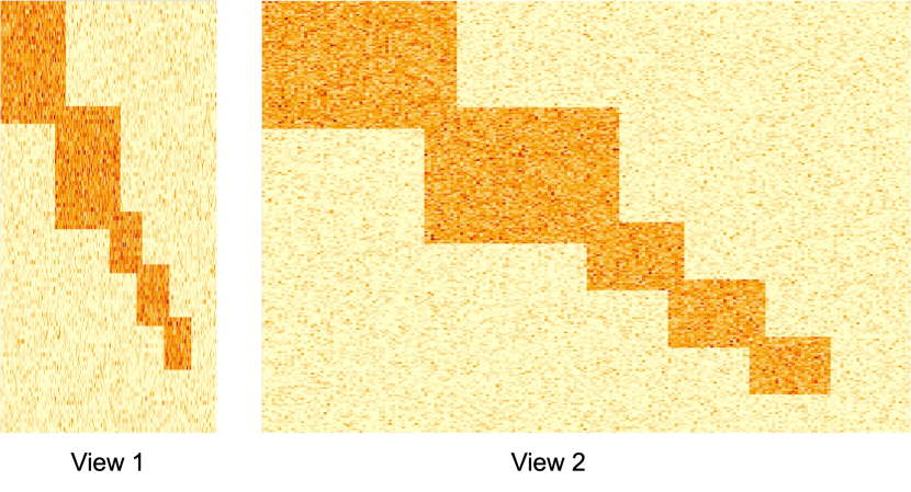
Figure 8: Synthetic data example with 5 overlapping and non-exhaustive biclusters. 2 views are present with 100 and 250 features in each view. A non-exhaustivity rate of 0.1 and an overlap rate of 0.2 are used.

B.3 Pre-processing steps

The pre-processing steps applied to the real datasets analysed in Section 5 are now detailed.

In all real datasets, only features with at least one non-zero element across the view are kept. A549 is the only dataset that received additional pre-processing steps. Genes in the scATAC-seq data with fewer than $5\%$ counts across cells and genes from the scRNA-seq data with standard deviation less than 0.4 were removed.

B.4 Hyper-parameter sensitivity

The biclusters are constructed to share common row clusters across rows and so restrictions between views are implemented via non-zero $\Phi$ with $\Psi=\Xi=0$. Each pairwise restriction has the same weighting i.e. all $\phi_{vw}=\phi$ for some constant $\phi$. A study into the performance of ResNMTF across various scenarios and varying values of the hyperpamater $\phi$ is conducted in this section. This allows us to select a single value of $\phi$ to be used across all studies concerning synthetic data in Section 5.

A base scenario, $S1$, of 2 views ($n_{r}=200$ and column dimensions $(100,250)$) and 4 biclusters with noise level $\sigma=3$ is considered. The number of biclusters is changed to 3 and 5 in scenarios $S2a$ and $S2b$ respectively. $S3$ increases the level of noise to $\sigma=6$ and $S4$ adds an additional view of dimensions $200\times 150$. Each scenario is repeated 100 times and results are averaged across all 500 repetitions. In order to gauge whether the restrictions between views has been implemented, the measure ’Restrictions‘ is defined and reported. For each repetition, this is a binary variable indicating whether or not the number of rows in the non-empty biclusters in view $v$ and $w$ are equal for all pairs $v$ and $w$. Whilst performance varies as $\phi$ changes, there are wide ranges of suitable values where the performance remains fairly constant and $\phi=200$ is selected as the value used in the synthetic data studies (Figure 9).

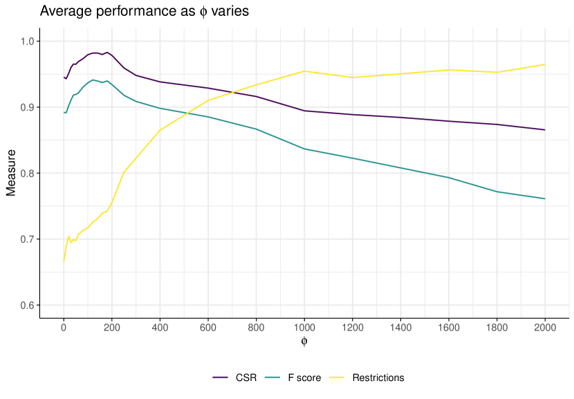
Figure 9: Results for averaged over 100 repetitions of $S1-S4$ with varying $\phi$.

Stability analysis is performed with $\omega=0.4$ (see Section 4.8 for the description of this hyperparameter). The value of $\omega$ applied on the synthetic datasets was selected based off preliminary investigations, however tuning of the stability analysis hyperparameter is investigated further on the real datasets in Figure 6(a).

B.5 Other methods

Here we detail the implementation of GFA by Bunte et al. [17] and iSSVD by Zhang et al. [16].

B.5.1 GFA

GFA is implemented via the ‘GFA’ package in R. As suggested in the package documentation, data is normalised using the ‘normalizeData’ function with ‘type’=center as a parameter. The prior is obtained with the ‘informativeNoisePrior‘ as prompted by the ‘gfa’ function if it implemented with the default prior. ‘getDefaultOpts’ function with ‘bicluster’=TRUE is used as the ‘opts’ parameter within ‘informativeNoisePrior’ alongside default values of ‘noiseProportion’=0.5 and ‘conf’=1.

B.5.2 iSSVD

With the default parameters as proposed in Zhang et al. [16], zero biclusters are detected in nearly all scenarios investigated with synthetic data in Section 5. In order to obtain biclusters, the following changes are made. Following the guided implementation in the packages Github page, the ‘ssthr’ parameter is set as $[0.6,0.65]$. The ‘row_overlap’ and ‘col_overlap’ parameters are set to ‘True’. The ‘pceru’ and ‘percv’ parameters which define the per-comparison wise error rate, controlling the number of falsely selected coefficients in the left and right singular vectors respectively, take values in $[0,1]$ and are changed from their default value of $0.1$ in order for iSSVD to return biclusters. As the choice of this parameter significantly affects performance, parameter optimisation is performed.

Results from an investigation into the performance of iSSVD on our synthetic data led to a per-comparison wise error rate of 0.7 being implemented across the synthetic data studies (Figure 10). Results for the investigation of this hyperparameter on data generated with a higher signal ($\mu=100$) further demonstrate the lack of suitability of the default parameter choice provided by the original authors (Figure 11). As Figure 11 suggests, it appears that whilst optimisation is necessary to improve the performance of iSSVD on the synthetic data, the main cause of the methods inability to detect biclusters is the low signal in the datasets. When the signal of the biclusters is increased (i.e. the mean of the Normal distribution elements are drawn from), the method is able to detect some biclusters (Figure 12). However, as demonstrated in Figures 12 and 13, this improvement in performance still appears to leave iSSVD inferior to both ResNMTF and NMTF. Additionally, Figures 12 and 13 highlight that the trends identified in 5 regarding the bisilhouette scores ability to preserve the ranks of the F-score largely remains as we increase the signal present in the data.

The presence of non-zero F-scores in the results of this section allow us to be satisfied that the poor performance seen by iSSVD in Section 5 is due to the methods inability to detect biclusters in the low signal setting and the requirement of hyperparameter tuning, rather than incorrect implementation.

As ResNMTF was applied with the same value of $\phi$ across all synthetic data scenarios, we believe the investigation detailed here demonstrates sufficient optimisation of iSSVD. Other parameters which have been changed are; ‘vthr’ which was set as [0.6, 0.65] (as opposed to the default [0.6,0.8]) for improved performance (as suggested on the package Github page ) and ‘col_overlap‘ and ‘row_overlap‘ which were both set to ‘True‘ as we want to allow for overlapping biclusters. The remainder of the parameters required for implementation of iSSVD take their default values; ‘standr’=False, ‘pointwise’=True, ‘steps’=100, ‘size’=0.5, ‘nbicluster’=10, ‘rows_nc’=True, ‘cols_nc’=True, ‘merr’=1e-4 and ‘iters’=100.

For implementation of iSSVD on the alternatively generated data in B.6.2, the parameters applied on the synthetic datasets in the original paper are used. The majority of these are the default values already mentioned, with the exception of ‘nbicluster’ which is set to 4. Similarly, for implementation of iSSVD on the real datasets, the parameter values applied on the real datasets in the original paper are used. The majority of these take the default value already mentioned, with the exception of ‘size’, ‘pceru’ and ‘pcerv’ which take 0.6, 0.15 and 0.16 respectively.

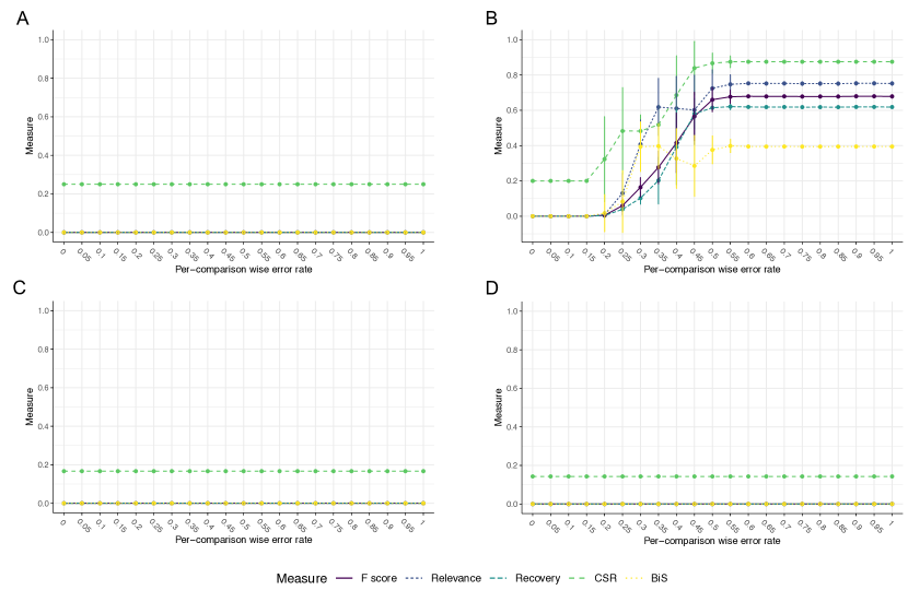
Figure 10: Results on iSSVD for increasing the ‘per-comparison wise error rate’ parameter, as described in Zhang et al. [16]. Applied on synthetic data (generated as described in Section 5.1) with 3 views (100, 50 and 250 columns), $\sigma=5$ and: (A) 3 ,(B) 4 (C) 5 and (D) 6 biclusters. The average score across 100 repetitions is reported with $\pm$ standard deviation error bars presented.

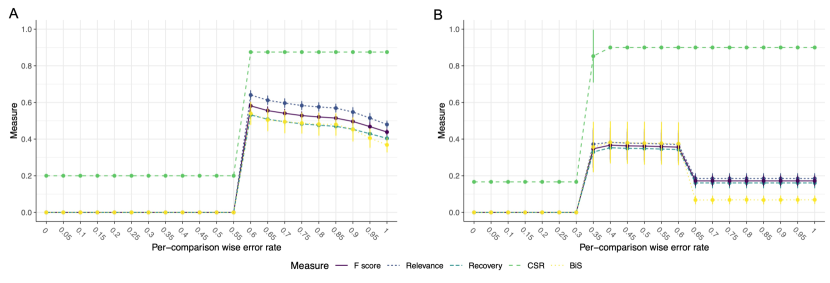
Figure 11: Results on iSSVD for increasing the ‘per-comparison wise error rate’ parameter, as described in Zhang et al. [16], on synthetic data with a larger signal. Applied on synthetic data (generated as described in Section 5.1) with 3 views (100, 50 and 250 columns), $\sigma=100$ and: (A) 4 and, (B) 5 biclusters. The average score across 100 repetitions is reported with $\pm$ standard deviation error bars presented.

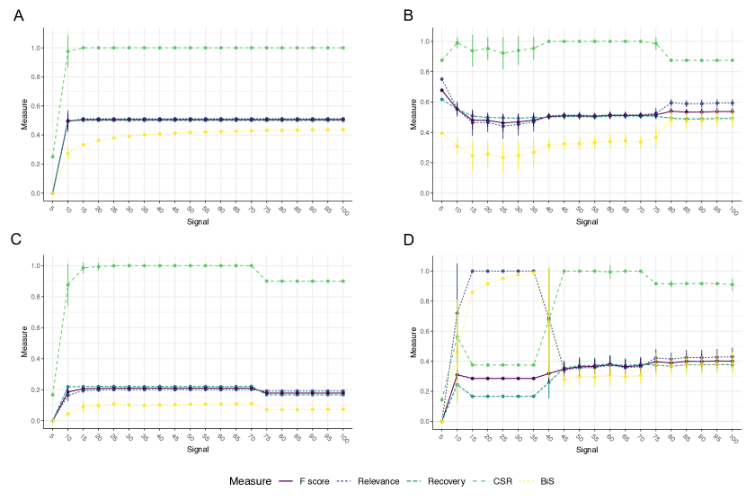
Figure 12: Results on iSSVD for increasing the signal ($\mu$) in synthetic data generated as described in Section 5.1. Applied on synthetic data with 3 views (100, 50 and 250 columns), $\sigma=5$ and: (A) 3, (B) 4, (C) 5 and (D) 6 biclusters. The average score across 100 repetitions is reported with $\pm$ standard deviation error bars presented.

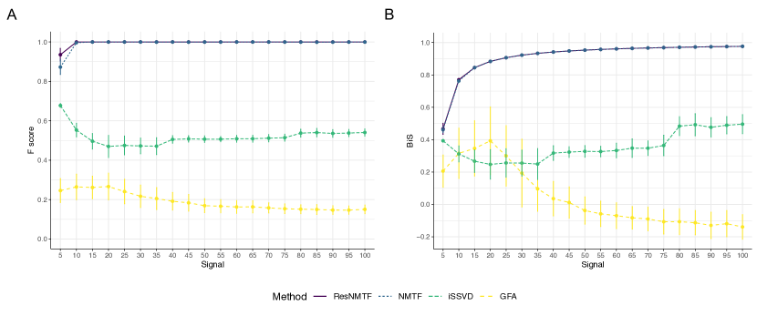
Figure 13: The effect of increasing the signal ($\mu$) in synthetic data (generated as described in Section 5.1) on the performance of methods. Applied on synthetic data with 3 views (100, 50 and 250 columns), $\sigma=5$ and 4 biclusters. The average A) F- and (B) bisilhouette scores across 100 repetitions are reported with $\pm$ standard deviation error bars presented.

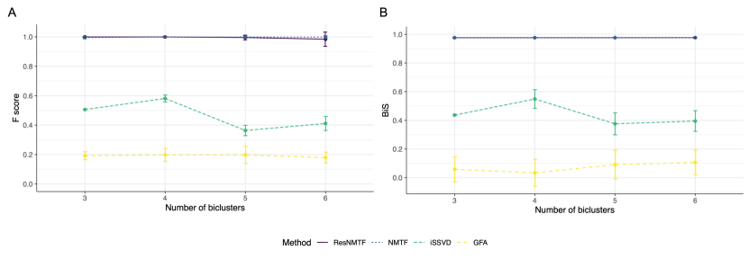
Figure 14: The effect of increasing the number of biclusters on (A) F- and (B) bisilhouette scores. The average scores across 100 repetitions are reported with $\pm$ standard deviation error bars presented. Data is generated with $\sigma=100$.

B.6 Further results

This section contains further experimental results. Additional results from the investigation of performance of the multi-view biclustering methods on synthetic data is presented in B.6.1. An alternative data generating process is then outlined and investigated presented in B.6.2. This is followed by an examination of different distance measures within the bisilhoutte score in B.6.3. Finally, visualisation plots using the silhouette score rather than the bisilhouette score are provided for comparison in B.6.4.

B.6.1 Auxiliary plots

Further results investigating the effect of various factors on the performance of ResNMTF when applied on synthetic data are included in this section. For all plots presented in this section, the data is generated as described in Section 5.1. When 2 views are present they have $100$ and $250$ features respectively (the smallest of the 3 ‘base’ views having been removed). When a fourth view is added to the base scenario, it contains $150$ features. An exception occurs when the study concerns the effect of increasing views. In this situation all views have $150$ features.

Figures 15, 14 and 17 all provide further evidence for the alignment between the F-score and the bisilhouette score of a result. In particular, in the experiment on the effect of increasing the number of views there is $100\%$ agreement between the rankings of the methods by the two scores. Figure 14 provides further evidence that the performance of ResNMTF falls when increasing the number of views. As the performance of NMTF does not fall to the same degree, this suggests the use of a sub-optimal restriction hyperparameter may be the cause. Whilst the performance of NMTF should be independent of the number of views when the number of features is constant across them, a slight drop in performance in NMTF between 2 and 4 views in Figure 14 is seen. This is likely caused by the introduction of a view with only 50 features.

Out of the methods considered, ResNMTF and NMTF are most affected by the increase (or simply presence) of the non-exhaustivity rate (Figure 17). However, the performance of these methods still remains superior to that of GFA and iSSVD.

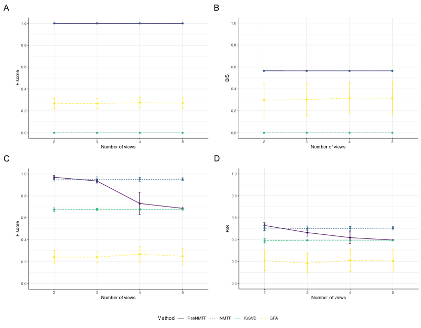
Figure 15: The effect of increasing the number of views on F-score (left column) and BiS (right column), with (A-B) 3 and (C-D) 4 biclusters. The average scores across 100 repetitions are reported with $\pm$ standard deviation error bars presented. Data is generated with $\sigma=5$.

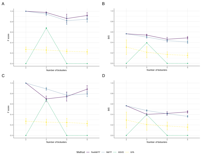
Figure 16: The effect of increasing the number of biclusters on F-score (left column) and BiS (right column), with (A-B) 2 and (C-D) 4 views. The average scores across 100 repetitions are reported with $\pm$ standard deviation error bars presented. Data is generated with $\sigma=5$.

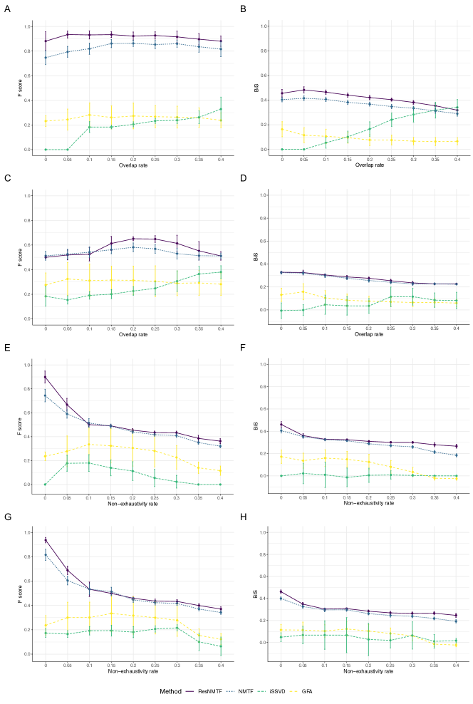
Figure 17: F-score (left column) and BiS (right column) for different methods: base scenario of 200 rows, 3 views (100, 50 and 250 columns), 5 biclusters and $\sigma=5$. The rate of overlap is varied on (A-B) exhaustive and (C-D) $10\%$ non-exhaustive biclusters. The rate of non-exhaustivity is varied on biclusters with (E-F) no overlap and (G-H) $10\%$ overlap. The average scores across 100 repetitions are reported with $\pm$ standard deviation error bars presented.

B.6.2 Alternative data generation

As well as generating synthetic data via the methods discussed in Section 5, data is generated as described in scenario 1, case 1 by Zhang et al. [16]. This study considers the relative scaling of views. The methods are performed on $\{X^{(1)},sX^{(2)}\}$ for different values of $s$, with $X^{(i)}$ generated by the same technique for both $i=1$ and $i=2$.

Figure 18 reproduces the performance of iSSVD demonstrated in the original paper, again verifying correct implementation of the method. The results demonstrate that all methods considered appear agnostic to scaling between views; this is to be expected for ResNMTF/NMTF as normalisation occurs. Additionally, alignment between the F-score and the bisilhouette score is once again seen. This is encouraging as it suggests the trends are not isolated to the original data structures considered. Whilst iSSVD outperforms the other methods in this study, the performance of ResNMTF/NMTF is still comparable to that of GFA.

Figure 18: Alternative data generation: the effect of increasing the scale of the second view on the (A) F-score and (B) BiS on data generated as outlined in scenario 1, case 1 inZhang et al. [16]. Each view has 4 biclusters. The average scores across 100 repetitions are reported with $\pm$ standard deviation error bars presented.

B.6.3 Distance measure

A preliminary investigation into the effect of the distance used within the bisilhouette score was conducted and the results are reported in Table 3. ResNMTF is applied on each of the real datasets with each of the following distances used within the bisilhouette score; Euclidean, cosine and Manhattan. Bisilhouette scores calculated using each distance are calculated over a range of restriction hyperparameter values, and the F-score corresponding to the maximal bisilhouette score for each specific distance is reported. For example, when considering the Euclidean distance used within the bisilhouette score within ResNMTF (i.e. to selet the number of biclusters), three scores will be reported, one for each distance used within the bisilhouette score in optimising the hyperparameter. For 3Sources and BBCSport $\psi\in(0,2000)$ is considered whilst $\phi\in(0,20000)$ is considered for A549. Five repeats are conducted with different random seeds and the result corresponding to the greatest F-score is reported. No stability selection is performed in any of the applications to better observe the effect of the different distances.

		3Sources			BBCSport			A549
		F-score	$\psi$	$k$	F-score	$\psi$	$k$	F-score	$\phi$	$k$
Euclidean	E	0.4496	1100	6	0.5221	200	9	0.4889	14000	3
	C	0.4518	1150	6	0.5635	250	8	0.3553	7000	3
	M	0.4496	1100	6	0.5221	200	9	0.4809	19000	3
	F	0.5071	1350	4	0.6247	600	7	0.5029	8500	3
Cosine	E	0.4563	1700	8	0.5975	1850	9	0.2781	6000	3
	C	0.4563	1700	8	0.5660	200	8	0.3606	0	3
	M	0.4563	1700	8	0.5975	1850	9	0.2781	6000	3
	F	0.5137	350	8	0.6247	600	7	0.3831	5500	3
Manhattan	E	0.4332	500	6	0.5670	100	8	0.4853	19500	3
	C	0.4359	400	6	0.5150	100	10	0.4393	12500	3
	M	0.4332	500	6	0.5150	100	10	0.4824	15000	3
	F	0.5191	1350	4	0.6223	500	6	0.5033	11500	3

Table 3: Results for using different distances to calculate the bisilhouette score within ResNMTF on the datasets. E/C/M denote selecting result by maximising bisilhouette with Euclidean/cosine/Manhattan distance to assess the final biclusterings. F denotes selecting via maximising F-score. The selected value of $\psi/\phi$ and the corresponding value of $k$ is reported. Five repeats are conducted.

B.6.4 Silhouette score

An investigation into the use of the original silhouette score to tune the restriction hyperparameter on the A549 dataset demonstrates the superiority of the bisilhouette score in conducting the same task (Figure 6(b)). The Pearson correlation between the F-score and the intrinsic measure falls from 0.867 to 0.711 when the silhouette score is used instead of the bisilhouette score.

References

- Pontes et al. [2015] B. Pontes, R. Giráldez, J. S. Aguilar-Ruiz, Biclustering on expression data: A review, J. of Biomed. Informatics 57 (2015) 163–180.
- Cheng and Church [2000] Y. Cheng, G. M. Church, Biclustering of expression data, Proc. of the Eighth Int. Conf. on Intell. Syst. for Mol. Biol. 8 (2000) 93–103.
- Dhillon [2001] I. S. Dhillon, Co-clustering documents and words using bipartite spectral graph partitioning, in: Proc. of the Seventh ACM SIGKDD Int. Conf. on Knowl. Discov. and Data Min., Assoc. for Comput. Mach., 2001, pp. 269–274.
- Denitto et al. [2017] M. Denitto, M. Bicego, A. Farinelli, M. Figueiredo, Spike and slab biclustering, Pattern Recognition 72 (2017) 186–195.
- Ding et al. [2006] C. Ding, T. Li, W. Peng, H. Park, Orthogonal nonnegative matrix t-factorizations for clustering, in: Proc. of the 12th ACM SIGKDD Int. Conf. on Knowl. Discov. and Data Min., Assoc. for Comput. Mach., 2006, pp. 126–135.
- Hwang et al. [2012] T. Hwang, G. Atluri, M. Xie, S. Dey, C. Hong, V. Kumar, R. Kuang, Co-clustering phenome–genome for phenotype classification and disease gene discovery, Nucleic Acids Res. 40 (2012) e146. doi:10.1093/nar/gks615.
- Xu et al. [2013] C. Xu, D. Tao, C. Xu, A survey on multi-view learning, 2013. URL: https://arxiv.org/abs/1304.5634. arXiv:1304.5634.
- Weinstein et al. [2013] J. N. Weinstein, E. A. Collisson, G. B. Mills, K. R. M. Shaw, B. A. Ozenberger, K. Ellrott, I. Shmulevich, C. Sander, J. M. Stuart, The cancer genome atlas pan-cancer analysis project, Nat. Genet. 45 (2013) 1113–1120.
- Rappoport and Shamir [2018] N. Rappoport, R. Shamir, Multi-omic and multi-view clustering algorithms: review and cancer benchmark, Nucleic Acids Res. 46 (2018) 10546–10562.
- Rodosthenous et al. [2020] T. Rodosthenous, V. Shahrezaei, M. Evangelou, Integrating multi-OMICS data through sparse canonical correlation analysis for the prediction of complex traits: a comparison study, Bioinform. 36 (2020) 4616–4625.
- Arya et al. [2023] N. Arya, S. Saha, A. Mathur, S. Saha, Improving the robustness and stability of a machine learning model for breast cancer prognosis through the use of multi-modal classifiers, Sci. Rep. 13 (2023) 4079.
- Rodosthenous et al. [2024] T. Rodosthenous, V. Shahrezaei, M. Evangelou, Multi-view data visualisation via manifold learning, PeerJ Comp. Sci. 10 (2024) e1993.
- von Luxburg [2010] U. von Luxburg, Clustering stability: An overview, Found. and Trends® in Mach. Learn. 2 (2010) 235–274. URL: http://dx.doi.org/10.1561/2200000008. doi:10.1561/2200000008.
- Horta and Campello [2014] D. Horta, R. J. G. B. Campello, Similarity measures for comparing biclusterings, IEEE/ACM Trans. Comput. Biol. Bioinform. 11 (2014) 942–954.
- Rousseeuw [1987] P. J. Rousseeuw, Silhouettes: A graphical aid to the interpretation and validation of cluster analysis, J. of Comput. and Appl. Math. 20 (1987) 53–65.
- Zhang et al. [2022] W. Zhang, C. Wendt, R. Bowler, C. P. Hersh, S. E. Safo, Robust integrative biclustering for multi-view data, Stat. Methods in Med. Res. 31 (2022) 2201–2216. doi:10.1177/09622802221122427.
- Bunte et al. [2016] K. Bunte, E. Leppäaho, I. Saarinen, S. Kaski, Sparse group factor analysis for biclustering of multiple data sources, Bioinform. 32 (2016) 2457–2463. doi:10.1093/bioinformatics/btw207.
- Sun et al. [2015] J. Sun, J. Lu, T. Xu, J. Bi, Multi-view sparse co-clustering via proximal alternating linearized minimization, in: F. Bach, D. Blei (Eds.), 32nd Int. Conf. on Mach. Learn., volume 37 of Proc. of Mach. Learn. Res., 2015, pp. 757–766.
- Nie et al. [2020] F. Nie, S. Shi, X. Li, Auto-weighted multi-view co-clustering via fast matrix factorization, Pattern Recognit. 102 (2020). doi:10.1016/j.patcog.2020.107207.
- Riddle-Workman et al. [2021] E. Riddle-Workman, M. Evangelou, N. M. Adams, Multi-type relational clustering for enterprise cyber-security networks, Pattern Recognit. Letters 149 (2021) 172–178.
- Meinshausen and Bühlmann [2010] N. Meinshausen, P. Bühlmann, Stability selection, J. of the Royal Stat. Soc.: Ser. B (Stat. Methodol.) 72 (2010) 417–473.
- Duan et al. [2021] R. Duan, L. Gao, Y. Gao, Y. Hu, H. Xu, M. Huang, K. Song, H. Wang, Y. Dong, C. Jiang, C. Zhang, S. Jia, Evaluation and comparison of multi-omics data integration methods for cancer subtyping, PLOS Comput. Biol. 17 (2021) 1–33.
- Padilha and de Leon Ferreira de Carvalho [2019] V. A. Padilha, A. C. P. de Leon Ferreira de Carvalho, Experimental correlation analysis of bicluster coherence measures and gene ontology information, Appl. Soft Comput. 85 (2019) 105688.
- Yip et al. [2004] K. Yip, D. Cheung, M. Ng, Harp: a practical projected clustering algorithm, IEEE Trans. on Knowl. and Data Eng. 16 (2004) 1387–1397. doi:10.1109/TKDE.2004.74.
- Akata et al. [2011] Z. Akata, C. Thurau, C. Bauckhage, Non-negative matrix factorization in multimodality data for segmentation and label prediction, in: 16th Comput. Vis. Winter Workshop, 2011, pp. 27–34.
- Liu et al. [2013] J. Liu, C. Wang, J. Gao, J. Han, Multi-view clustering via joint nonnegative matrix factorization, in: Proc. of the 2013 SIAM Int. Conf. on Data Min. (SDM), 2013, pp. 252–260. URL: https://epubs.siam.org/doi/abs/10.1137/1.9781611972832.28. doi:10.1137/1.9781611972832.28.
- He et al. [2014] X. He, M.-Y. Kan, P. Xie, X. Chen, Comment-based multi-view clustering of web 2.0 items, in: Proc. of the 23rd Int. Conf. on World Wide Web, WWW ’14, Assoc. for Comput. Mach., 2014, pp. 771–782. doi:10.1145/2566486.2567975.
- Yang et al. [2018] L. Yang, L. Zhang, Z. Pan, G. Hu, Y. Zhang, Community detection based on co-regularized nonnegative matrix tri-factorization in multi-view social networks, 2018 IEEE Int. Conf. on Big Data and Smart Comput. (BigComp) (2018) 98–105.
- Zhang et al. [2019] J. Zhang, Y. Rao, J. Zhang, Y. Zhao, Trigraph regularized collective matrix tri-factorization framework on multiview features for multilabel image annotation, IEEE Access 7 (2019) 161805–161821.
- Vavasis [2010] S. A. Vavasis, On the complexity of nonnegative matrix factorization, SIAM J. on Optim. 20 (2010) 1364–1377.
- Lin [2007] C.-J. Lin, On the convergence of multiplicative update algorithms for nonnegative matrix factorization, IEEE Trans. on Neural Netw. 18 (2007) 1589–1596.
- Long et al. [2005] B. Long, Z. M. Zhang, P. S. Yu, Co-clustering by block value decomposition, in: Proc. of the Eleventh ACM SIGKDD Int. Conf. on Knowl. Discov. in Data Min., KDD ’05, Assoc. for Comput. Mach., 2005, pp. 635–640.
- Lee and Seung [2000] D. Lee, H. S. Seung, Algorithms for non-negative matrix factorization, Adv. in Neural Inf. Process. Syst. 13 (2000).
- Čopar et al. [2019] A. Čopar, B. Zupan, M. Zitnik, Fast optimization of non-negative matrix tri-factorization, PLOS ONE 14 (2019) 1–15.
- Boutsidis and Gallopoulos [2008] C. Boutsidis, E. Gallopoulos, Svd based initialization: A head start for nonnegative matrix factorization, Pattern Recognit. 41 (2008) 1350–1362.
- Lin [1991] J. Lin, Divergence measures based on the shannon entropy, IEEE Trans. on Inf. Theory 37 (1991) 145–151.
- Duong-Trung et al. [2019] N. Duong-Trung, M.-H. Nguyen, H. T. H. Nguyen, Clustering stability via concept-based nonnegative matrix factorization, in: Proc. of the 3rd Int. Conf. on Mach. Learn. and Soft Comput., ICMLSC ’19, Assoc. for Comput. Mach., New York, NY, USA, 2019, pp. 49–54.
- Jaccard [1901] P. Jaccard, Etude de la distribution florale dans une portion des alpes et du jura, Bull. de la Soc. Vaud. des Sci. Nat. 37 (1901) 547–579.
- Cao et al. [2018] J. Cao, D. A. Cusanovich, V. Ramani, D. Aghamirzaie, H. A. Pliner, A. J. Hill, R. M. Daza, J. L. McFaline-Figueroa, J. S. Packer, L. Christiansen, F. J. Steemers, A. C. Adey, C. Trapnell, J. Shendure, Joint profiling of chromatin accessibility and gene expression in thousands of single cells, Sci. 361 (2018) 1380–1385.
- Verma et al. [2015] N. K. Verma, E. Dutta, Y. Cui, Hausdorff distance and global silhouette index as novel measures for estimating quality of biclusters, in: 2015 IEEE Int. Conf. on Bioinform. and Biomed. (BIBM), 2015, pp. 267–272. doi:10.1109/BIBM.2015.7359691.
- HG [2018] D. HG, Philentropy: Information theory and distance quantification with r, J. of Open Source Softw. 3 (2018) 765.
- Santamaría et al. [2007] R. Santamaría, L. Quintales, R. Therón, Methods to bicluster validation and comparison in microarray data, in: H. Yin, P. Tino, E. Corchado, W. Byrne, X. Yao (Eds.), Intell. Data Eng. and Autom. Learn. - IDEAL 2007, Springer Berl. Heidelberg, 2007, pp. 780–789.