Measuring the Effect of Transcription Noise on
Downstream Language Understanding Tasks

Abstract

With the increasing prevalence of recorded human speech, spoken language understanding (SLU) is essential for its efficient processing. In order to process the speech, it is commonly transcribed using automatic speech recognition technology. This speech-to-text transition introduces errors into the transcripts, which subsequently propagate to downstream NLP tasks, such as dialogue summarization. While it is known that transcript noise affects downstream tasks, a systematic approach to analyzing its effects across different noise severities and types has not been addressed. We propose a configurable framework for assessing task models in diverse noisy settings, and for examining the impact of transcript-cleaning techniques. The framework facilitates the investigation of task model behavior, which can in turn support the development of effective SLU solutions. We exemplify the utility of our framework on three SLU tasks and four task models, offering insights regarding the effect of transcript noise on tasks in general and models in particular. For instance, we find that task models can tolerate a certain level of noise, and are affected differently by the types of errors in the transcript.

Measuring the Effect of Transcription Noise on
Downstream Language Understanding Tasks

Ori Shapira, Shlomo E. Chazan,  and Amir DN Cohen OriginAI oris@originai.co

1 Introduction

Human speech is captured by microphones constantly. Dialogues or utterances are recorded at online meetings, for creating content, and for being aided by virtual assistants or service providers. Many of these recordings inevitably require automated processing, for which the common approach is to run automatic speech recognition (ASR) systems that convert audio to transcribed text. The produced transcript is then handled with spoken language understanding (SLU) technology.

Considerable effort is invested in developing ASR systems that can overcome environmental sounds, vague speech and phenomena of spoken language, in order to produce transcripts that are as faithful to the speech (“clean”) as possible (Iwamoto et al., 2022; Prabhavalkar et al., 2023). In turn, the text processing step can be performed more effectively. Simply put, the mistakes (“noise”) produced in the speech-to-text stage propagate to downstream tasks in the text processing stage (Kubis et al., 2023; Feng et al., 2022a).

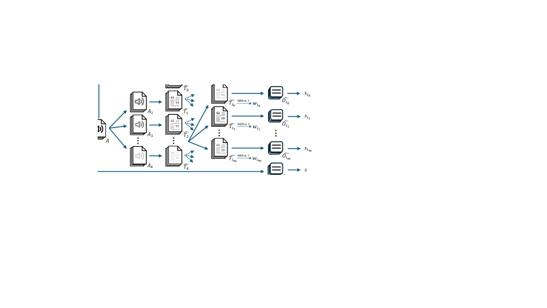
Figure 1: Speech can be transcribed with varying levels of error severity, which effects the results of downstream language understanding tasks. For example, summarizing a transcript with variations of the utterance above might produce differing outcomes. The top version is the reference, and the following are marked with errors.

Eventual SLU tasks are abundant, from traditional dialog act classification (Shriberg et al., 2004) to summarization (Waibel et al., 1998) and even neurological assessment of speakers (Roshanzamir et al., 2021). Indeed, over the years studies have noticed that noisy transcripts burden NLP models, and actions are consequently taken to work around or mitigate the noise (surveyed in Section 2). Furthermore, different downstream tasks are not alike in how they respond to the amount and types of errors in transcripts. Some are highly vulnerable to errors, while others may tolerate more noise, or specific types of noise, depending on a task’s requirements (as demonstrated in our analyses in Section 5). Figure 1 shows an utterance transcribed with varying levels of error severity, causing unpredictable behavior in downstream understanding tasks. Importantly, the standard word error rate (WER) metric, that measures the amount of errors in generated transcripts, does not capture discrepancies in types of noise, and cannot forecast results on downstream tasks (Wang et al., 2003).

Drawing upon lessons from previous research on SLU, in this work we propose a framework for systematically analyzing the effect of transcription noise on a downstream task (ENDow; Section 3). Our first-of-its-kind framework examines task model behavior under varying noise intensities and types, providing quantitative metrics and facilitating qualitative analyses. It determines acceptable noise levels for a downstream task, identifies effective transcript-cleaning techniques, and supports planning and implementation of SLU solutions. Previous studies have examined aspects of ENDow, but always within the scope of a specific task or use case. We suggest that, especially in the era of generalized models and benchmarks, there is a need for a versatile framework that consistently analyzes and compares SLU solutions. The components in the framework’s pipeline, such as the ASR system or task model, are flexibly configured to perform controlled examinations.

Given an SLU dataset, the framework prepares audio files, with varying levels of acoustic distortion, which are then transcribed by an ASR system, producing transcript sets with increasing levels of transcription noise. A method of transcript cleaning then adjusts noise types, generating additional transcript versions. Finally, a downstream task model is applied, allowing comparison and analysis across the transcript versions. Notably, beyond its configurable pipeline, the framework supports any task dataset, including non-spoken language datasets, greatly expanding the scope for assessing ENDow.

We exemplify the use of our framework (Section 4), and perform an extensive analysis (Section 5) across three SLU tasks, with seven intensities of noise, seven cleaning techniques, and four LLM task models. Specifically, we focus on summarization (Zhong et al., 2021), question-answering (Wu et al., 2022), and dialog-act classification (Shriberg et al., 2004), all from existing SLU datasets.

The results of our diversified experiments yield many insights regarding the level of noise that is acceptable for the downstream tasks, and the impact of the type of errors in the transcripts. For example, we observe that named entities are usually the most important term-types for dealing with the tasks, while, surprisingly, verbs are seemingly not as essential. Some findings are unique to specific tasks and models, while others are more consistent. For instance, it is apparent in our experiments that there is a certain amount of noise from which it is not worth the trouble of reducing it. However, that intensity fluctuates with respect to the task, the model, and the type of noise. The framework also reveals phenomena that occur at particular noise levels, as well as gradual changes as noise increases. For example, we find that GPT-4o-mini (OpenAI, 2024) outperforms other models on summarization when transcript noise is low, but the other models overtake GPT as noise increases. Such findings are valuable for identifying commonalities and differences among various SLU configurations, helping to prioritize efforts for achieving satisfactory outcomes on a downstream task.

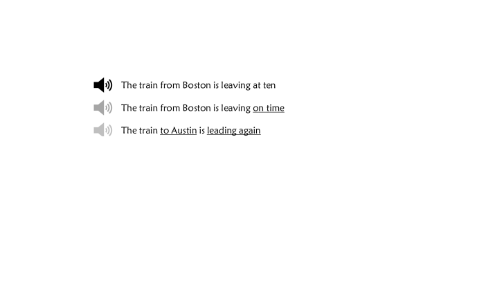
Figure 2: The pipeline of the ENDow framework which yields a downstream task score and a WER score of the transcript set input to the task. The pipeline is executed for several severeties of noising and types of cleaning techniques. Resulting scores are plotted on a graph for the analyses, as in, e.g., Figure 4.

2 Background and Related Work

Spoken language understanding (SLU; Wang et al., 2005) commonly refers to a set of applicative tasks performed on speech (Feng et al., 2022a; Shon et al., 2023). A prevalent approach for SLU is to transcribe speech with ASR systems, and to process the text with Natural Language Understanding (NLU) techniques that extract meaning from it (Tur and De Mori, 2011).

Spoken language does not usually obey standard syntactic rules and contains disfluencies such as repairs and hesitations (Wang et al., 2005). Moreover, when recording speech, the distance of a microphone, the clarity of speech, and environmental sounds add challenging hurdles for an ASR system, that hence produce transcripts that are unfaithful to the spoken words. The discrepancies between the reference (gold) transcript and the automatically produced transcript, a.k.a. “noise”, is most commonly measured with word error rate (WER). This metric measures the percentage of words in the ASR-transcript that were wrongly inserted, substituted and deleted, with respect to the reference transcript, i.e., a form of word edit distance.

To decrease the WER scores or improve subsequent results on downstream tasks, one line of work focuses on correcting ASR-generated transcripts, e.g., by correcting spelling (Guo et al., 2019; Dutta et al., 2022), disfluencies (Stouten et al., 2006), punctuation (Di Gangi et al., 2019), or mistakes in general (Leng et al., 2021; Guo et al., 2023). However, no cleaning method is flawless, and the errors in the transcript propagate on to the NLU stage (Errattahi et al., 2018). Additionally, studies (Gopalakrishnan et al., 2020; Kim et al., 2021) argue that NLU models are mainly trained on written language and are not robust for spoken language, let alone for erroneous spoken language. Therefore, some works train proprietary models for downstream tasks with noisy transcripts to improve results, e.g., for machine translation, intent classification, question answering, and more (Fang et al., 2020; Cui et al., 2021; Liu et al., 2021; Feng et al., 2022b; Jung et al., 2024).

Another track of research analyzes the influence of transcript noise on tasks such as summarization (Szaszák et al., 2016; Tündik et al., 2019; Chowdhury et al., 2024), question-answering (Lee et al., 2018; You et al., 2021) and classification (Shon et al., 2022; Steven J. Pentland and Twitchell, 2023), mainly by comparing results with and without transcript noise in the input. To expand this analysis, there are works that assess downstream results at several levels or types of noise (Zechner and Waibel, 2000; Agarwal et al., 2007; Gopalakrishnan et al., 2020; Feng et al., 2022a; Shon et al., 2023; Li et al., 2024). Some add noise synthetically to reference transcripts, while a few prepare recordings with impaired clarity (Feng et al., 2022a) or use back-transcription (Kubis et al., 2023). Controlling the types of noise reveals their effect (Balagopalan et al., 2020; Min et al., 2021), working around the limitations of the WER metric, that does not account for the type of words or their importance to the task (Wang et al., 2003). User studies were similarly set up in order to assess how well humans conduct tasks on noisy transcripts (Stark et al., 2000; Sanders et al., 2002; Munteanu et al., 2006; Favre et al., 2013). They often find at which WER score the ability of users to consistently complete tasks starts to deter.

The studies described above aim to analyze the effect of transcription noise on downstream tasks, however each concentrates on a specific setting and employs different practices. Our proposed framework generalizes a method for conducting such assessments, allowing systematic examination of SLU pipelines. Furthermore, although there are few works (Li et al., 2023; Zhu et al., 2024) that analyze the ability of GPT-family LLMs to handle short transcribed texts on SLU tasks (e.g., ASR-GLUE; Feng et al., 2022a), ours is the first, to the best of our knowledge, to assess the performance of several recent LLMs on full dialogues of spoken language. Regardless, our framework is robust to any form of dialogue, NLU task, and task model.

3 A Framework for Measuring ENDow

With the purpose of systematically analyzing SLU pipelines, our framework’s objective is to describe the behavior of downstream tasks as a function of the noise score (e.g., WER, which we use throughout the paper, but any transcription noise metric can be applied) and the type of noise in transcripts.

The input to the framework is an SLU dataset $D=(T,O)$, where $T$ is a set of reference transcripts and $O$ are the respective expected outcomes. For example, a set of meetings and their respective summaries, for the task of meeting summarization.

The framework consists of a pipeline (illustrated in Figure 2) which includes a text-to-speech (TTS) model to generate audio files for $T$; the acoustic noising method and intensity to apply on the audio; an ASR system for audio transcription; the transcript cleaning technique; the downstream task model; and the evaluation metrics for the task. The components in the pipeline are flexibly set according to the use-case being analyzed.

The framework outputs a report on the behavior of the SLU pipeline at the different noise levels and with the cleaning techniques assessed (§3.3).

3.1 Preparing Transcripts with Varying Noise

Creating initial audio files.

Audio files are first created for the input transcripts, in case the SLU dataset lacks them (or when using a non-SLU dataset), or to begin the analysis with clean audio for greater control over the subsequent noising process. The TTS system is executed on each input (transcript) in dataset $D$, resulting in the corresponding set of audio files $A$.

Adding noise to audio files.

Given the audio files $A$, each is acoustically impaired at $k$ levels to increase transcription difficulty, preferably under realistic acoustic conditions. To that end, reverberation (i.e., sound reflection, like echoing) is applied, and background sounds are added with increasing intensity (signal-to-noise ratio) (Wang and Chen, 2018). This stage yields a collection of audio sets $\{A_{i}\}_{i=1}^{k}$ (and we define $A_{0}=A$), where the severity of impairment increases as $i$ increases.

Transcribing audio files.

The ASR model is then executed on the audio files in sets $\{A_{i}\}_{i=0}^{k}$, resulting in respective transcripts $\{\widehat{T_{i}}\}_{i=0}^{k}$. Overall, there are $k+2$ sets of transcripts for dataset $D$: the $k+1$ ASR-generated sets and reference set $T$. It is expected that as $i$ increases, $\widehat{T_{i}}$ will have a higher WER score (more errors) with respect to $T$.

Cleaning transcripts.

Each non-reference transcript (in all sets $\widehat{T_{i}}$) is partially repaired using one of $m$ cleaning techniques. This culminates in sets $\{\{\widehat{T_{i_{j}}}\}_{j=1}^{m}\}_{i=0}^{k}$, and $\widehat{T_{i_{0}}}=\widehat{T_{i}}$ (when no cleaning is performed on $\widehat{T_{i}}$), encompassing $(k+1)*(m+1)$ different levels and types of transcript noise.

3.2 Executing the Downstream Task

Next, the task model is executed on each of the transcripts in the prepared transcript sets, producing the respective predicted outputs $\{\{\widehat{O_{i_{j}}}\}_{j=0}^{m}\}_{i=0}^{k}$, and $\widehat{O}$ for the reference transcripts $T$. The predicted outputs in each set $\widehat{O_{i_{j}}}$ and $\widehat{O}$ are then evaluated against the respective expected outcomes in $O$. Finally, this process culminates with the overall score of each dataset variant $\{\{s_{i_{j}}\}_{j=0}^{m}\}_{i=0}^{k}$ and $s$.

In addition, the WER score is computed for each transcript set $\widehat{T_{i_{j}}}$ with respect to references $T$. Accordingly, this produces WER scores $\{\{w_{i_{j}}\}_{j=0}^{m}\}_{i=0}^{k}$ (see Appendix A.1 for details). Notice that $T$’s WER is $0$. With the task scores and respective WER scores, we can now assess and compare the performance of the dataset variants.

3.3 Analyzing the Results

Each of the WER and task score-pairs $(w_{i_{j}},s_{i_{j}})$ is a data point that can be plotted on a graph. The curve $l_{j}=[(0,s)]\cdot[(w_{i_{j}},s_{i_{j}})]_{i=0}^{k}$ describes the behavior of a task model as noise increases in the transcripts (as $i$ increases), when applying cleaning technique $j$ (or when no cleaning is enforced, at $j=0$). These curves form a basis for analyzing the configured SLU pipeline, as explained next. (See Figure 5 in the Appendix for visualization.)

Model performance vs. noise level.

As transcript noise accumulates, NLU task model performance is expected to degrade. One question to ask is: how much transcript noise can the task model tolerate before its performance is jeopardized? To that end, we define the noise-toleration point (NTP) as follows. For curve $l_{j}$, described by function $f_{j}$, and the respective upper and lower bound functions $f_{j}^{\text{upper}}$ and $f_{j}^{\text{lower}}$ (based on the margins-of-error), we define $l_{j}$’s noise-toleration point, $w^{t}_{j}$, as the WER score when $f_{j}^{\text{lower}}(0)=f_{j}^{\text{upper}}(w^{t}_{j})$, i.e., the lowest WER at which the task score becomes statistically significantly lower than when transcripts have no noise, indicating a notable drop in task-model performance due to noise.

Another question to ask about the SLU pipeline is: how do different models behave comparatively, with respect to noise level? The general behavior is approximated with the area-under-the-curve (AUC), which can be compared between curves to judge which model is generally more tolerant to noise. Furthermore, by focusing on a certain region in the graph, the localized behavior is comparable. For example, in Figure 3a, the GPT model is the better model at lower WER levels, but drops to the bottom rank at high WER levels.

Comparing cleaning techniques.

Applying a cleaning technique on transcripts decreases the noise, and consequently shifts the plots leftward. Cleaning a transcript also essentially means that the type of noise changes, and therefore the task model reacts differently to the errors in the transcripts, potentially altering the behavior of the curves altogether. The point $(w_{i_{j}},s_{i_{j}})$ with respect to point $(w_{i_{0}},s_{i_{0}})$ portrays how much “effort” is required (the decrease in WER: $w_{i_{0}}-w_{i_{j}}$) in order to change the task score from $s_{i_{0}}$ to $s_{i_{j}}$. The effect of each cleaning method $j$ varies, and therefore all $l_{j}$s are compared with respect to $l_{0}$ (e.g., see Figure 4). Ultimately, an effective cleaning technique should increase the task scores with minimum effort.

Formally, let $\Delta w_{i_{j}}=w_{i_{0}}-w_{i_{j}}$ be the change in WER for noising level $i$ and cleaning method $j$, and $\delta s_{i_{j}}=(s_{i_{0}}-s_{i_{j}})/s$ be the respective relative change in the task-score. The pointwise effectiveness score of cleaning technique $j$ at noise-level $i$ is measured as $e_{i_{j}}=\delta s_{i_{j}}/\sqrt{\Delta w_{i_{j}}+\epsilon}$. Finally, we measure the cleaning-effectiveness score (CES) of cleaning method $j$ with the average: $\frac{1}{k+1}\sum_{i=0}^{k}e_{i_{j}}$. The higher the score, the better the overall improvement in the downstream task with a lower effort of cleaning. A score of 0 means that the cleaning procedure had no effect on the task-model’s results, and a negative score means that there was a deterioration of task results, on average.

The CES metric captures the two objectives of a cleaning technique: heightened task results for lesser effort. The metric suggests how comparably effective a cleaning method is for the data and task-model in question. As such, it compares the effects of different types of noise in the transcripts, as we exemplify in our experiments in Section 5.

4 Experimental Setup

Task	Dataset Source	Task Type	Granularity Level	Domains	Evaluation Metrics	# Transcripts	# Instances	# Utts. in Inst. Avg. (min - max)
Summarization (Generic + Query Focused)	QMSum	Generation	Transcript	Product, Research, Parliament meetings	Pairwise Ranking, ROUGE-1,2,L	35	281	592 (131 - 1368)
Question Answering	QAConv	Extraction	Transcript	Court cases, Interviews	Fuzzy match, Exact, Token-level $F_{1}$	505	2083	104 (5 - 585)
Dialog Act Classification	MRDA	Classification	Utterance	Research meetings	Macro-$F_{1}$, Accuracy	12	1200	1

Table 1: The test data with which we conduct our experiments, with varying input/output formats and speech domains. # Instances refers to queries for summarization, questions for QA, and utterances for dialog-act classification.

To demonstrate the utility of the framework for measuring ENDow, we describe the various SLU pipeline configurations on which we apply the framework and conduct analyses (discussed in §5).

4.1 Preparing Transcript Sets

Text-to-speech model.

Some of the SLU datasets in our experiments lack accompanying audio files, and in any case, we would like our experiments to be based on a controlled speech environment. We used the toirtoise-tts (Betker, 2023) Python library as the text-to-speech model, and implemented a procedure for handling lengthy speech (see Appendix A.3). The TTS stage produces the initial set of audio files for each of the SLU datasets in our experiments.

Noising method.

Each audio file was reverberated with the rir-generator (Werner, 2023) Python library, and then recreated with background office sounds (a clipped audio file; myNoise, 2020) with one of five signal-to-noise ratios (see Appendix A.4). After this process there are six sets of increasingly tampered audio files.

ASR system.

We used Whisper (Radford et al., 2023) for conducting speech-to-text (see Appendix A.5). In all there are seven sets of increasingly noised transcripts (the first is the clean reference set). In our setting, seven noise levels provided a satisfactory analysis for examining the behavior of the SLU pipeline. The WER scores distribute within 0 and 0.9, and the curves empirically exhibit sufficiently clear behavioral patterns.

Cleaning techniques.

In our experiments, we use the cleaning component to study the effect of different types of words, e.g., nouns, on downstream tasks. This analysis also simulates an SLU pipeline in which the ASR system prioritizes accuracy for specific word types, guiding where to focus efforts in the transcription process.

To clean transcripts, we first aligned a noised transcript to its respective reference transcript with jiwer. Then, any non-equivalent alignment that involves the targeted word-type was repaired. We separately target nouns, verbs, adjectives, adverbs, any of the above (“content words”), none of the above (“non-content words”), and named entities – seven techniques in all. Details in Appendix A.6.

4.2 Downstream Tasks

We experiment with three downstream tasks, characterized by different output objectives. Summarization is a generation task where text is synthesized based on the collective understanding of a dialog. Question-answering is framed here as an extraction task that retrieves spans from the transcript. Dialog-act categorization is a classification task that assigns a communicative goal label (e.g., ‘statement’, ‘question’, etc.) to conversational utterances. The first two tasks are on the full transcript level, while the latter task is on the utterance level. These differences offer insights into potential distinctions in SLU pipelines.

In our experiments we focus on long spoken dialogues, as opposed to short or written dialogues, as they impose a more challenging setting for task models. See Table 1 for a summary of the tasks, and Appendix E for examples of task instances.

Summarization.

For summarization, we use the QMSum dataset (Zhong et al., 2021), a generic and query-focused dialog summarization benchmark. It consists of transcripts and summaries of product meetings (AMI; Carletta et al., 2006), academic meetings (ICSI; Janin et al., 2003) and parliament committee meetings.

To evaluate system summaries we use standard ROUGE metrics (Lin, 2004) and pairwise comparison ranking (Qin et al., 2024) with GPT-4o-mini as a judge for overall quality (Liu et al., 2024) (see Appendix A.7 for details).

Question-answering.

The QAConv dataset (Wu et al., 2022) consists of dialogues with questions whose answers are short spans in the dialog. We only use the instances based on court cases or interviews (since these are long spoken dialogues).

For evaluation, predicted answers are compared against reference answers with exact match accuracy, token-level $F_{1}$ and fuzzy matching, following the QAConv benchmark.

Dialog-act classification.

The MRDA dataset (Shriberg et al., 2004) consists of meetings from the ICSI corpus and research-oriented group meetings. Each utterance in the transcripts is labeled with one of 12 dialog act labels (Dhillon et al., 2004). We utilize the first and last 50 utterances from each transcript (100 of $\sim$1392), for efficiency purposes. See Appendix E for more details.

The MRDA results were traditionally evaluated with the accuracy metric, but we also evaluate with macro-$F_{1}$ due to the high class imbalance in the dataset, as suggested by Miah et al. (2023).

Models.

For all three tasks, we experiment with four instruct-tuned LLMs in zero-shot mode: Mistral-7B, Llama3-8B, Llama3.1-8B, and GPT-4o-mini. They were selected for their modest hardware requirements and affordability. Since the context size of Mistral and Llama-3 cannot fit most of the transcripts in full, summarization and QA were conducted on these models in segments. See details and prompts in Appendix B.

5 Results and Analyses

(a) QMSum with pairwise ranking evaluation

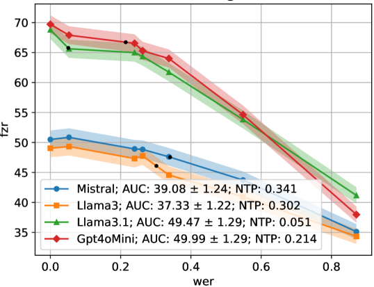
(b) QAConv with fuzzy match evaluation

(c) MRDA with macro-$F_{1}$ evaluation

Figure 3: Model performance on the experimented tasks. Curves are compared with area-under-the-curve (AUC) and noise-toleration points (NTP; marked with black dots). NTP marks the WER value where the task-score first decreases significantly from the score at $\text{WER}=0$. A line’s shaded area represents its confidence interval. Graphs for the rest of the metrics are in Figure 6.

Our experiments include the configurations described in Section 4, with results discussed here.

Comparing task models.

The following analyses reveal how task models perform under varying levels of noise. The AUC and NTP scores provide a high-level comparison for assessing ENDow, while the graph curves illustrate model behavior as noise fluctuates.

Figure 3 presents the results on the three downstream tasks for the four models, based on one of the evaluation metrics per task. In the summarization task results (Figure 3a) we first notice that models tend to tolerate a noise level of about 0.2 WER (NTP between 0.07 and 0.3), i.e., task scores are not significantly lower ($p<0.05$) until that level of noise. Also, while the AUC scores for all models are not significantly different ($p<0.05$), models behave differently with respect to WER. For example, GPT’s summaries are more highly preferred at lower WER than at higher WER values, while for Mistral, the preference is slightly more evenly distributed.

In the question-answering task (Figure 3b), the more advanced models (GPT and Llama-3.1) yield substantially better results than the other two models. This could be an effect of the small context window which requires conducting the task in segments, likely inducing more errors. Similar to the behavior in summarization, here too GPT yields better scores than Llama 3.1 at low WER, but Llama 3.1 surpasses GPT as WER increases.

In the dialog-act classification task (Figure 3c), the noise-toleration points are quite high due to the large margins-of-error and relatively flat curves. A high NTP either implies that noise has little effect on a downstream task, or alternatively that the model is ineffective for the task in general. In this case, the latter seems to be the case, when comparing to results of Miah et al. (2023) ($0.29$ macro-$F_{1}$ and $0.6$ accuracy vs. $[0.17,0.32]$ macro-$F_{1}$ and $[0.3,0.48]$ accuracy here). More in Appendix D.

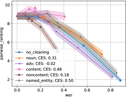
(a) QMSum with pairwise ranking evaluation, for GPT

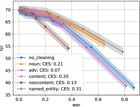
(b) QAConv with fuzzy matching evaluation, for GPT

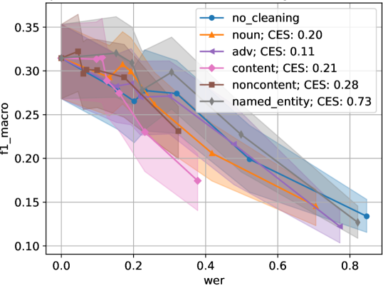
(c) MRDA with macro-$F_{1}$ evaluation, for GPT

Figure 4: The performance of GPT-4o-mini when applying various cleaning techniques. Compare a point on the “no_cleaning” curve to the respective point on a cleaning technique’s curve. Effective cleaning means maximizing gain in task score (y-axis) with minimum effort (x-axis), measured using the cleaning-effectiveness score (CES). Additional CES scores are in Table 2, and more graphs are in Figures 7, 8 and 9 in the Appendix.

		Mistral	Llama3	Llama3.1	GPT4oMini
QMSum | PW-Rank	Named-ents	0.537	1.346	0.193	0.499
	Content	0.322	0.581	0.357	0.479
	Nouns	0.459	0.804	0.384	0.305
	Non-content	0.262	0.480	0.209	0.181
	Adjectives	0.327	1.216	0.230	0.135
	Verbs	0.229	0.702	0.145	0.073
	Adverbs	0.223	0.956	0.017	-0.023
QAConv | Fuzzy	Named-ents	0.221	0.469	0.294	0.311
	Nouns	0.164	0.280	0.210	0.211
	Content	0.108	0.224	0.186	0.202
	Non-content	0.070	0.177	0.094	0.133
	Adjectives	-0.037	0.398	0.109	0.120
	Verbs	-0.012	0.188	0.059	0.090
	Adverbs	0.004	0.335	0.033	0.071
MRDA | Mac-$F_{1}$	Named-ents	-0.035	-0.049	-0.291	0.735
	Adjectives	0.404	-0.001	0.035	0.290
	Non-content	0.392	0.122	0.122	0.285
	Content	0.315	0.027	-0.053	0.212
	Nouns	0.010	0.102	-0.042	0.203
	Verbs	0.044	-0.024	-0.232	0.158
	Adverbs	-0.043	-0.085	-0.342	0.107

Table 2: The cleaning-effectiveness scores (CES) of the experimented cleaning techniques on the four task-models. Techniques ordered for each task by ranking on GPT model (corresponding graphs in Figure 4). Full table for all task-metrics in Table 4 in the Appendix.

Comparing noise types.

The following analyses highlight the impact of different types and intensities of noise. This examination enables more efficient optimization of ASR systems and post-hoc transcript repair. For instance, as the analysis will show, prioritizing named-entity accuracy may be more effective than generally minimizing the WER of the ASR system.

Figure 4 presents the graphs showing the effect of cleaning techniques on the performance of GPT (graphs for the rest of the models and cleaning techniques in Figures 7, 8 and 9 in the Appendix). The “no cleaning” curve shows model results on the transcripts at the various noise levels. The other curves on the graph show model results when also applying a cleaning technique on the same transcripts.

In the summarization task (Figure 4a), fixing all the content words in the transcripts (“content” curve) helps the model produce summaries that are preferred over all the summaries that are based on the original transcripts, regardless of noise level. However, due to this technique’s costly “effort” (high change in WER), the cleaning-effectiveness score (0.479) is not as high as that of the “named entities” technique (0.499). The latter cleaning method improves the task scores at a smaller cost of effort on average, as depicted in the graph. These findings indicate the value of content words, and named entities in particular, for the summarization task using GPT. Notice that transcripts that are almost fully error-prone (WER is $\sim$0.9) are fixed to a WER of $\sim$0.4 by repairing content words, but resulting summaries are much preferred over summaries from transcripts with different types of errors, also at a WER of 0.4. This further stresses the importance of analyzing the types of errors in transcripts and not just the amount, which is a known limitation of the WER metric.

Table 2 lists the CES scores of each model and cleaning technique, ranked by the effectiveness on GPT. For the QA task, we see that the cleaning techniques are ranked quite similarly across the four task-models. In all three tasks, fixing only adverbs or verbs is less effective. On the other end, nouns, and named-entities particularly, are more effective for the transcript-level tasks (summarization and QA). The utterance-level task of dialog-act classification behaves differently with respect to the repaired word-types. Interestingly, repairing non-content words is effective for the task, consistent with works that found that function words are essential features for classifying dialog-acts (O’Shea et al., 2012; Jo et al., 2017). Named-entities are also effective for the task with GPT. A closer look into the graph (Figure 4c) reveals that the high CES is affected by the behavior at lower WER scores, where a strong increase in the task score is obtained at a small effort.

6 Conclusion

Errors in speech-to-text automation propagate to downstream language understanding tasks, with noise magnitude and type affecting tasks and models differently. We present a configurable framework for evaluating noise impact, enabling analysis of model behavior across noise levels and transcript-cleaning techniques. Extensive experiments demonstrate its utility, providing insights into task model performance in SLU. The framework’s flexibility supports more effective comparison and development of SLU pipelines.

Limitations

In our experiments, the pipelines are initiated with relatively clean and clear audio files, and the subsequent acoustic deterioration is done in a specific manner (reverberation and background sounds). Other acoustic settings are indeed possible for initiating the SLU pipeline, e.g., with a low-resourced lingual dialect, different speaker voices per turn, overlapping speech, microphone settings, and many other parameters. Our framework is robust to these variants, and the purpose of our experiments is to exemplify the utility of the framework.

Similarly, our experiments are limited to the configurations we defined, for demonstrating the framework. Other configurations could involve non-English languages, different tasks, models and SLU/NLU datasets. The resulting analyses could yield findings that are different from ours, which reiterates the need for a robust framework like ours.

The cleaning techniques we used depend on the reference transcript in order to identify the word/phrase types that we want to include in our analysis. Our experiments show how different types of errors affect a downstream task. A cleaning technique can also be one that is used in practice without dependence on the reference transcript. In the latter case, our framework would indicate the effectiveness of a transcript-cleaning component within an SLU pipeline.

We emphasize that the behavior of a graph depends on the task metric applied, and the resulting analysis can therefore differ when using different metrics for the same task and data. When insights are gathered with the framework, it is important to strongly consider the metric used, or use several metrics to paint a fuller picture.

Appendix A Implementation Details

A.1 Computing Overall WER on a Set of Transcripts

Before computing WER, the utterances in a transcript are tokenized using spaCy (Honnibal and Montani, 2017), and then the tokens are recombined with separating spaces. This is done mainly to separate punctuation and contractions.

The WER score for a transcript is computed against the reference transcript using the jiwer.process_words function. It computes hits, insertions, substitutions and deletions between each predicted and respective reference utterance. Then all of the utterance level values are added up, and a single WER score is computed accordingly for the transcript.

Once the transcript-level WER scores are computed, the transcript-set WER score is the average over all transcripts in the set.

A.2 Computing the Noise-toleration Point (NTP)

Observe Figure 5 for a visualization of the following explanation. The computation of the noise-toleration point of a curve $l_{j}$ relies on $l_{j}^{\text{upper}}$ and $l_{j}^{\text{lower}}$, the lines with the respective margins-of-error. The y-value, i.e., task score, of each point in $l_{j}^{\text{upper}}$ ($l_{j}^{\text{lower}}$) is the upper (lower) limit margin-of-error for the corresponding point’s y-value in $l_{j}$. Specifically, task score $s_{i_{j}}$, as part of point $(w_{i_{j}},s_{i_{j}})$ on $l_{j}$, is the average task score over the transcripts in the set $\widehat{T_{i_{j}}}$, and the respective margin-of-error is computed at a confidence level of $95\%$ with the formula $1.96*\sigma/\sqrt{n}$, where $\sigma$ is the standard deviation of the scores, and $n$ is the number of scores (number of transcripts). The x-values on $l_{j}^{\text{upper}}$ and $l_{j}^{\text{lower}}$ are kept the same as in the respective points on $l_{j}$. With these margins-of-error line, we can compute the NTP.

Since a model’s curve $l_{j}$ is constructed of several discrete points, we find the first point $p_{i}:=(w_{i_{j}},s_{i_{j}})$ in $l_{j}$ whose upper bound (based on the margin-of-error) is above the lower bound of the first point $p_{0}$, and where the next point $p_{i+1}$ has an upper bound that is below $p_{0}$’s lower bound. Then on the linear segment between $p_{i}$ and $p_{i+1}$, we find the $x$ value (WER score) where its upper bound is equal to the lower bound of $p_{0}$.

Figure 5: An illustration of the graph generated with the framework, for visual reference.

A.3 Executing Text-to-speech

To create the initial audio files from the dataset transcripts, we first removed substrings in the utterances that are within curly and box brackets. These are used in some transcripts to indicate non-verbal markers. We also removed redundant whitespaces. An utterance was sentence-tokenized (with nltk.tokenize.sent_tokenize), and then also broken up to segments of up to 50 tokens, if it was longer than that (with nltk.tokenize.word_tokenize). We found that in some cases the TTS module had some difficulty in voicing more than 50 tokens at a time (more than about 15 seconds of speech). Each segment was then passed to tortoise.api.TextToSpeech and an audio file was created with the “emma” voice in “ultra_fast” mode, and saved with a 24000 sample frequency.

A.4 Impairing Audio Files

An audio file is recreated $k$ times at increasing levels of speech deterioration. First the audio file is reverberated once using the Room Impulse Response Generator (rir_generator library; Werner, 2023). Then background sounds are added at $k$ different signal-to-noise ratios, as described below.

The reverberation parameters are as follows. The room dimensions are uniformly selected for each of width (2 to 10 meters), length (2 to 10 meters) and height (exactly 3 meters). Assuming that the room is enclosed by walls, a floor and a ceiling, the speaker position is uniformly selected for each of x-position (somewhere 0.5 meters from the wall), y-position (somewhere 0.5 meters from the wall), and z-position (somewhere between the floor and the ceiling). The microphone location is randomly placed 2 meters away from the speaker if it’s within the bounds of the room, otherwise 1 meter away, otherwise 0 meters away. The Reverberation Time (RT60 – the time it takes for sound energy to decrease by 60 dB after the sound source stops) is uniformly selected between 0.15 and 1 second. Sound velocity is kept at the default value of 340 meters per second. The sample frequency is kept at the original value (24000 samples per second).

To the resulting reverberated audio file denoted signal, background sounds are added at $k$ different signal-to-noise ratios (SNR – level of a desired signal to the level of background noise). First a sound audio file (myNoise, 2020) denoted noise_signal (in our case we used an office background that includes realistic sounds such as chatter, papers, office machinery, drinking, etc.) is loaded, and repeated so that its length is equal to that of the speech audio file, or truncated to that length. The resulting background file is denoted white_noise. Then the noise factor is computed according to the SNR with:

$$g=\sqrt{\frac{10^{-\texttt{SNR}/10}*\text{std}(\texttt{signal})^{2}}{\epsilon+\text{std}(\texttt{noise\_signal})^{2}}}$$

The final audio file is created as:

$$\texttt{noisy\_signal}=\texttt{signal}+g*\texttt{white\_noise}$$

The $k$ SNR values that we use in our experiments are -10, -5, 0, 5, 10. The higher the value, the more distinctive the speech is over the background noise.

A.5 Executing ASR for Speech-to-text

To run Whisper on a transcript, a Huggingface (Wolf et al., 2020) automatic-speech-recognition pipeline is initialized with the openai/whisper-small.en model. The pipeline receives each audio file and generates the respective text. Since our audio files are up to about 15 seconds in length and mostly under 1MB in size, the model is able to handle the files properly.

A.6 Cleaning Transcripts

Our cleaning techniques rely on the reference transcripts, and therefore are used to inidicate how different types of errors effect the behavior of a model on a downstream task.

Given a chunk of 20 utterances from the predicted transcript, and the respective chunk from the reference transcript, spaCy is used to tag the part-of-speech labels of each token, and the named entity chunks. Then jiwer.process_words is used to align the texts. For each alignment, if there is a substitution, addition or deletion, and it involves a type (POS or named entity) that is being cleaned, then that alignment is fixed.

As mentioned, we separately clean each of: nouns, verbs, adjectives, adverbs, all the above (content words), none of the above (non-content words) and named entities.

An example for cleaning nouns (in bold):

Reference: “We certainly see it, as employers. The penny drops after a few weeks or months.”

Noisy: “We certainly seen it as lawyers. The penny drops after the new songs.”

Cleaned: “We certainly seen it as employers . The penny drops after the new weeks months.”

A.7 Pairwise Ranking for Summarization Evaluation

Pairwise comparison has been shown to be highly effective for judging the overall quality of summaries (Liu et al., 2024) using gpt-4-0314 as a judge. We use a presumably more advanced model (gpt-4o-mini), and assume high reliability.

Given two competing summaries, the reference summary, and an optional query on which the summary is focused, a pairwise comparer needs to mark the preferred summary (in our case, for “general quality”). The two summaries being compared are presented to the comparer in random order to remove an order bias with regard to the preference made. We use a method inspired by the LLMCompare protocol from Liu et al. (2024).

For a generic summary we input the following prompt to gpt-4o-mini:

For a query-focused summary we input the following prompt to gpt-4o-mini:

Pairwise ranking for non-cleaned versions.

A non-cleaned transcript-set is prepared at seven levels of noise (no noise, and six levels of increasing intensity). These are marked as $T$ (the reference transcript set) and $\{\widehat{T_{i_{0}}}\}_{i=0}^{k}$ (noisy versions) respectively. The resulting summary sets are denoted $\widehat{O}$ (on the reference transcripts $T$) and $\{\widehat{O_{i_{0}}}\}_{i=0}^{k}$. Then the summaries for instance $z$, i.e., $\widehat{o_{i_{0}}^{z}}\in\widehat{O_{i_{0}}}$ and $\widehat{o^{z}}\in\widehat{O}$ (seven summaries total) are compared in pairs through the pairwise compairson LLM annotation. In all there are 21 pairs, and the preferred summary receives 2 points, or 1 point for a tie. Hence, a summary that is preferred over all other six summaries can score a maximum of 12 points, and a total of 42 points are distributed amongst the seven summaries. The scores for each noise version are averaged over all instances of the test set (281 instances), and margin-of-errors are computed. These scores are then plotted on the curve, e.g., as in Figure 3a.

Using the Azure OpenAI API, the cost for computing all comparisons for one model was about $1.50. For the four models this process totalled about $6.

Pairwise ranking for cleaning techniques.

For a cleaning technique $j$, a summary $\widehat{o_{i_{j}}^{z}}\in\widehat{O_{i_{j}}}$ is instead compared to summaries $\widehat{o_{i_{0}}^{z}}\in\widehat{O_{i_{0}}}$ and $\widehat{o^{z}}\in\widehat{O}$. In this case, we want to assess how the cleaned summary compares against the non-cleaned summaries. Each of the six cleaned summaries is compared against seven non-cleaned summaries, for a total of 42 comparisons per instance. A summary can score up to 14 points, and 84 points are distributed amongst the compared summaries. The scores for the cleaned summaries are avarged over all instances of the test set (281 instances), and margin-of-errors are computed. These scores are then plotted on the curve, e.g., as in Figure 4a. In this graph, the non-cleaned line is reused from the non-cleaned pairwise ranking from before, except that it is shifted up one point in the y-axis. This is done as if to emulate the same procedure done here where the non-cleaned summaries should be compared to all the non-cleaned summaries (including itself), and would hence receive an additional point for the tie of a summary against itself.

Using the Azure OpenAI API, the cost for computing all comparisons for one model and one cleaning method was about $4.30. For the four models and seven cleaning techniques, this amounted to about $120.

Appendix B Executing Task Models

The four LLMs in our experiments were executed in zero-shot mode. mistral-7b, llama-3-8b and llama-3.1-8b were run on a local server. gpt-4o-mini was run with the Azure OpenAI API.

The summarization and question-answering tasks are given a transcript in the input. The transcripts and therefore chunked to fit (with the instruction) the context window of the employed model. For mistral-7b and llama-3-8b the size is 8K, for llama-3.1-8b and gpt-4o-mini it is 128K. The latter two models do not require chunking for our tested data. The prompts were scripted with some light prompt engineering on a few instances.

B.1 Summarization with QMSum

The prompt for summarizing the full transcript is:

The prompt for summarizing the transcript in segments is:

and the segment summaries are then summarized into one final summary with:

Notice that the prompt is phrased as if the query is a question and the summary is an answer. This layout is used to adhere to QMSum’s format. The query for all the generic summaries is “Summarize the meeting”. An example query for a query-focused summary is “What was the next step on features?” or “Summarize what was said on intentionality”.

The approximate cost for inferring on the QMSum test set with gpt-4o-mini was $0.30.

B.2 Question-answering with QAConv

For question-answering, the following prompt is input to the LLM:

The transcript is chunked to fit within the context window of the LLM. Therefore, after answering the questions a chunk at a time, the final answer for a question is the shortest answer that is not “unanswerable”. The default answer is “unanswerable” if no other answer is available.

The approximate cost for inferring on the QAConv test set with gpt-4o-mini was $0.25.

B.3 Dialog-act Classification with MRDA

The prompt for classifying dialog acts is:

The approximate cost for inferring on the MRDA test set with gpt-4o-mini was $0.10.

Appendix C Compute and Hardware

For the components of the pipeline that require it, we use a single Nvidia A100 GPU with 40GB memory. This is needed for running Tortoise TTS, Whisper STT and for running open-source task models (Mistral and Llama models). The rest of the components run on an Apple M1 Macbook.

Appendix D More Results from Experiments

The graphs presented in Section 5 only show results when using pairwise comparison for summarization evaluation, fuzzy match for QA evaluation, and macro-$F_{1}$ for dialog act classification evaluation. Here we present the results also for the rest of the evaluation metrics for the three tasks.

Comparing task models.

Figure 6 presents the graphs based on the rest of the task evaluation metrics, including those already presented in Figure 3. Table 3 places the AUC and noise-toleration point scores for each curve in a single table for readability. The highest AUC score in each row is in bold, to show the task model achieving the best result. Significance can be inferred with the margin-of-errors.

For summarization, we find that the AUC scores do not differ significantly across models in all metrics, with the exception of Llama-3.1 having the highest AUC when using ROUGE-2 as the metric. The ROUGE metrics in general produce large margin-of-errors, causing comparison between models to be more vague. We do however notice that Llama-3.1 yields a larger difference in results as WER increases, when using all summarization metrics. We also see a consistent trend in Llama-3 where there seems to be a sudden drop and gain around a WER of 0.2.

The three metrics used for QAConv are quite consistent. For MRDA, we find that the accuracy metric raises the ranking of the Mistral model, since Mistral was always more likely to output a label of a prevalent class, stressing the advantage of the macro-$F_{1}$ metric that balances the importance of the classes.

For MRDA, we compare in Section 5 results to those in Miah et al. (2023). They use an even more fine-grained label set (53 vs. 12 labels), yet still produce better scores overall. This further strengthens our presupposition that the models in our experiments are not as effective on the task, resulting in high noise-toleration-points on the curves.

Comparing noise types.

Figures 7, 8 and 9 show the graphs based on the rest of the task models, evaluation metrics, and cleaning techniques, including those in Figure 4. Table 4 shows all the cleaning effectiveness scores accordingly, similar to Table 2, but with the cleaning techniques kept in consistent order.

When looking at the cleaning-effectiveness scores, we find that ROUGE-2 ranks the cleaning techniques closest to the way that pairwise ranking does. In QAConv, the $F_{1}$ metric ranks the cleaning techniques very similarly for all four models. With the exception of Llama-3, the rankings are similar also with the exact and fuzzy matching metrics as well. For MRDA, although the score values are quite different, the rankings are close when using the two evaluation metrics.

As discussed in Section 5, generally the named-entities and nouns are most helpful for the summarization and question-answering tasks. For GPT, this is also the case for dialog-act classification, however with the open-source models, the non-content words are most helpful for the task.

		Mistral-7B		Llama3-8B		Llama3.1-8B		GPT-4o-mini
	Metric	AUC	NTP	AUC	NTP	AUC	NTP	AUC	NTP
QMSum	PW-Rank	5.817 ± 0.321	0.195	5.811 ± 0.331	0.070	5.746 ± 0.312	0.249	5.627 ± 0.280	0.297
	R-1	0.227 ± 0.008	-	0.228 ± 0.008	0.487	0.210 ± 0.010	0.526	0.225 ± 0.008	-
	R-2	0.051 ± 0.004	0.631	0.048 ± 0.004	0.460	0.062 ± 0.006	0.494	0.051 ± 0.004	0.598
	R-L	0.143 ± 0.005	-	0.147 ± 0.005	0.586	0.140 ± 0.007	0.517	0.138 ± 0.005	-
QAConv	Fuzzy	39.080 ± 1.241	0.341	37.331 ± 1.217	0.302	49.466 ± 1.288	0.051	49.992 ± 1.286	0.214
	$F_{1}$	0.289 ± 0.015	0.324	0.255 ± 0.014	0.269	0.384 ± 0.016	0.037	0.392 ± 0.016	0.050
	Exact	0.179 ± 0.015	0.293	0.164 ± 0.014	0.273	0.277 ± 0.017	0.031	0.291 ± 0.017	0.042
MRDA	Mac-$F_{1}$	0.110 ± 0.019	0.560	0.149 ± 0.028	0.615	0.140 ± 0.028	0.709	0.193 ± 0.032	0.439
	Acc	0.331 ± 0.023	-	0.263 ± 0.023	0.841	0.253 ± 0.022	0.790	0.371 ± 0.024	0.553

Table 3: The area-under-the-curve (AUC; with margin of error at 95% confidence level) and the noise-toleration point (NTP) of the experimented task models on the three tasks (summarization, question-answering and dialog-act classification). The highest AUC in each row is in bold. The scores correspond to the graphs in Figure 6, where a more in-depth examination can be conducted.

		Mistral	Llama3	Llama3.1	GPT4oMini
QMSum | PW-Rank	Adjs.	0.327	1.216	0.230	0.135
	Advs.	0.223	0.956	0.017	-0.023
	Content	0.322	0.581	0.357	0.479
	N-ents.	0.537	1.346	0.193	0.499
	Non-cont,	0.262	0.480	0.209	0.181
	Nouns	0.459	0.804	0.384	0.305
	Verbs	0.229	0.702	0.145	0.073
QMSum | R-1	Adjs.	-0.068	0.237	-0.038	0.071
	Advs.	-0.071	0.203	-0.058	0.059
	Content	-0.006	0.119	0.078	-0.003
	N-ents.	-0.085	0.198	-0.005	-0.115
	Non-cont,	-0.028	0.090	0.043	0.033
	Nouns	-0.038	0.145	0.058	0.057
	Verbs	-0.074	0.103	-0.003	0.062
QMSum | R-2	Adjs.	0.000	0.403	0.054	0.198
	Advs.	-0.084	0.422	0.011	0.134
	Content	0.053	0.234	0.212	0.249
	N-ents.	-0.093	0.492	0.140	0.265
	Non-cont,	0.003	0.188	0.104	0.101
	Nouns	0.028	0.327	0.252	0.189
	Verbs	-0.131	0.208	0.066	0.156
QMSum | R-L	Adjs.	-0.092	0.189	-0.015	0.050
	Advs.	-0.100	0.136	-0.014	0.054
	Content	-0.022	0.083	0.081	0.008
	N-ents.	-0.120	0.144	0.014	-0.052
	Non-cont,	-0.038	0.061	0.049	0.018
	Nouns	-0.040	0.120	0.088	0.041
	Verbs	-0.081	0.065	0.031	0.057
QAConv | Fuzzy	Adjs.	-0.037	0.398	0.109	0.120
	Advs.	0.004	0.335	0.033	0.071
	Content	0.108	0.224	0.186	0.202
	N-ents.	0.221	0.469	0.294	0.311
	Non-cont,	0.070	0.177	0.094	0.133
	Nouns	0.164	0.280	0.210	0.211
	Verbs	-0.012	0.188	0.059	0.090
QAConv | $F_{1}$	Adjs.	-0.376	-0.050	0.175	0.145
	Advs.	-0.276	0.063	0.020	0.102
	Content	0.152	0.304	0.318	0.325
	N-ents.	0.271	0.584	0.510	0.493
	Non-cont,	0.070	0.204	0.192	0.227
	Nouns	0.203	0.372	0.378	0.347
	Verbs	-0.095	0.085	0.110	0.134
QAConv | Exact	Adjs.	-0.003	0.948	0.221	0.225
	Advs.	-0.049	0.852	0.014	0.141
	Content	0.329	0.573	0.391	0.399
	N-ents.	0.657	1.162	0.692	0.688
	Non-cont,	0.215	0.462	0.221	0.284
	Nouns	0.423	0.728	0.477	0.438
	Verbs	0.001	0.441	0.131	0.170
MRDA | Mac-$F_{1}$	Adjs.	0.404	-0.001	0.035	0.290
	Advs.	-0.043	-0.085	-0.342	0.107
	Content	0.315	0.027	-0.053	0.212
	N-ents.	-0.035	-0.049	-0.291	0.735
	Non-cont,	0.392	0.122	0.122	0.285
	Nouns	0.010	0.102	-0.042	0.203
	Verbs	0.044	-0.024	-0.232	0.158
MRDA | Acc	Adjs.	-0.335	-0.619	-0.366	0.174
	Advs.	-1.160	-1.035	-0.887	-0.207
	Content	-0.373	-0.362	-0.350	-0.082
	N-ents.	-1.087	-0.797	-0.618	0.245
	Non-cont,	-0.685	-0.431	-0.386	-0.081
	Nouns	-0.594	-0.437	-0.314	-0.047
	Verbs	-0.654	-0.584	-0.436	-0.179

Table 4: The cleaning-effectiveness scores (CES) of the experimented cleaning techniques on the four task-models. In the experimented techniques, a certain group of words is repaired, with respect to the reference transcripts, in so demonstrating the effect of varying noise types. The corresponding graphs are shown in Figures 7, 8 and 9.

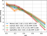
(a) QMSum with pairwise ranking

(b) QMSum with ROUGE-1

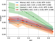
(c) QMSum with ROUGE-2

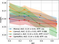
(d) QMSum with ROUGE-L

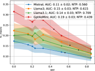
(e) MRDA with macro-$F_{1}$

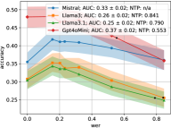
(f) MRDA with accuracy

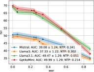
(g) QAConv with fuzzy match

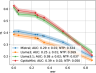
(h) QAConv with token $F_{1}$

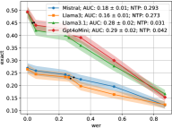
(i) QAConv with exact match

Figure 6: The performance of the models on the tasks in our experiments. The curves provide insights into the performance of the models at various noise levels. The curves in each plot can be compared with their area-under-the-curve. Also, each curve is marked with its noise-toleration point, which provides the WER value where the task-score first decreases significantly, with respect to the score at $\text{WER}=0$. The shaded area around a line represents the corresponding confidence interval. The scores can be found in Table 3.

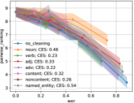
(a) Pairwise ranking, Mistral

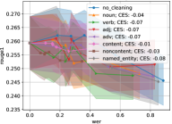
(b) ROUGE-1, Mistral

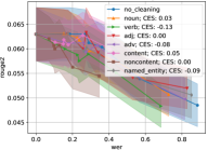
(c) ROUGE-2, Mistral

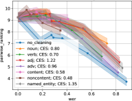
(d) Pairwise ranking, Llama3

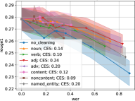
(e) ROUGE-1, Llama3

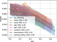
(f) ROUGE-2, Llama3

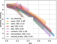
(g) Pairwise ranking, Llama3.1

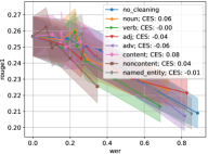
(h) ROUGE-1, Llama3.1

(i) ROUGE-2, Llama3.1

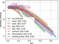
(j) Pairwise ranking, GPT

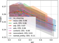
(k) ROUGE-1, GPT

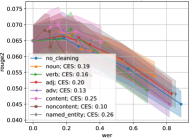
(l) ROUGE-2, GPT

Figure 7: The performance of models when applying various cleaning techniques, on the summarization dataset of QMSum. Each point on the “no_cleaning” curve can be compared to the respective point on a cleaning technique’s curve. A good cleaning technique should increase the task score (y value) as much as possible, with as little effort as possible (represented by decrease in WER, as the x value). Each cleaning technique is marked with its overall cleaning-effectiveness score which is computed as a function of the change in the task score and in the WER score. The CES scores can be seen also in Table 4.

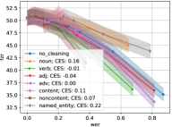
(a) Fuzzy match, Mistral

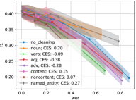
(b) Token $F_{1}$, Mistral

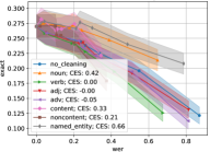
(c) Exact match, Mistral

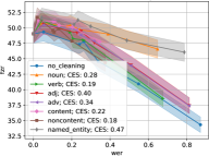
(d) Fuzzy match, Llama3

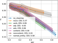
(e) Token $F_{1}$, Llama3

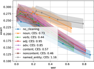
(f) Exact match, Llama3

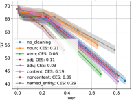
(g) Fuzzy match, Llama3.1

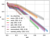
(h) Token $F_{1}$, Llama3.1

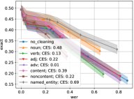
(i) Exact match, Llama3.1

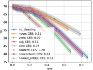
(j) Fuzzy match, GPT

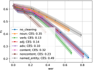
(k) Token $F_{1}$, GPT

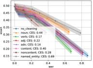
(l) Exact match, GPT

Figure 8: The performance of models when applying various cleaning techniques, on the question-answering dataset of QAConv. Each point on the “no_cleaning” curve can be compared to the respective point on a cleaning technique’s curve. A good cleaning technique should increase the task score (y value) as much as possible, with as little effort as possible (represented by decrease in WER, as the x value). Each cleaning technique is marked with its overall cleaning-effectiveness score which is computed as a function of the change in the task score and in the WER score. The CES scores can be seen also in Table 4.

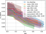
(a) Macro-$F_{1}$, Mistral

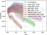
(b) Accuracy, Mistral

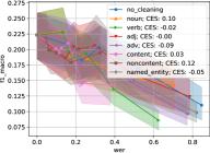
(c) Macro-$F_{1}$, Llama3

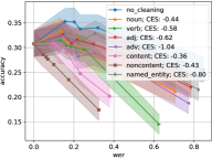
(d) Accuracy, Llama3

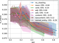
(e) Macro-$F_{1}$, Llama3.1

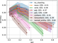
(f) Accuracy, Llama3.1

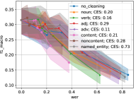
(g) Macro-$F_{1}$, GPT

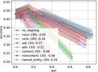
(h) Accuracy, GPT

Figure 9: The performance of models when applying various cleaning techniques, on the dialog-act classification dataset of MRDA. Each point on the “no_cleaning” curve can be compared to the respective point on a cleaning technique’s curve. A good cleaning technique should increase the task score (y value) as much as possible, with as little effort as possible (represented by decrease in WER, as the x value). Each cleaning technique is marked with its overall cleaning-effectiveness score which is computed as a function of the change in the task score and in the WER score. The CES scores can be seen also in Table 4.

Appendix E Task Datasets and Example Instances

QMSum.

An example of an instance for summarization from the QMSum dataset is in Figure 10.

QAConv.

An example of an instance for question-answering from the QAConv dataset is in Figure 11.

MRDA.

Examples of instances for dialog act classification from the MRDA dataset are in Figure 12.

The label-sets in dialog-act classification vary from one dataset to another, and have different levels of granularity (from 5 to 50+ labels). The utterances in MRDA are labeled with a dialog act on three granularity levels (with tag-sets of 5, 12 or 53 labels). For our experiments, we used the middle granularity level (tagset with 12 dialog acts; Dhillon et al., 2004), and the first and last 50 utterances from each transcript (100 of $\sim$1392), for efficiency purposes.

Figure 10: An example from the QMSum dataset. Each of the 35 transcripts has a generic summary and several query-focused summaries (avg. 8 summaries per transcript).

Figure 11: An example from the QAConv dataset, from which we only use the long spoken conversations. Each of the 505 transcripts has several questions (avg. 4.1) whose answers are extracted from the transcript. A question can have one or more answers (separated by a “|” in the figure), or it can be unanswerable.

Figure 12: A snippet from a transcript in the MRDA dataset. Each utterance has at least one segment, and each segment (beginning with the underlined speaker ID) is labeled with its dialog act in bold. There are 12 transcripts, and we use a subset of 100 utterance segments per transcript for a total of 1200 instances.

Appendix F Licenses

The following are the licenses of the used resources:

• Corpora:

  • QMSum: MIT

  • QAConv: BSD-3-Clause (Salesforce)

  • MRDA: GPL-3.0

• Tools:

  • tortoise-tts: Apache-2.0

  • rir-generator: MIT

  • jiwer: Apache-2.0

  • spacy: MIT

• LLMs: Mistral and Llama models are gated models pulled from Huggingface.

We use the above resources for exemplifying our framework, and solely for research purposes. Generally, our framework is intended for assessment of SLU solutions.

The code for our framework and analyses will be released under the Apache-2.0 license.

Appendix G Use of AI for the Paper

ChatGPT was used for some minor rephrasing of sentences within the paper, and for assisting in preparing code to programmatically fill tables in LaTeX (placing results in tables for the paper).

References

- Agarwal et al. (2007) Sumeet Agarwal, Shantanu Godbole, Diwakar Punjani, and Shourya Roy. 2007. How Much Noise Is Too Much: A Study in Automatic Text Classification. In Seventh IEEE International Conference on Data Mining (ICDM 2007), pages 3–12.
- Balagopalan et al. (2020) Aparna Balagopalan, Ksenia Shkaruta, and Jekaterina Novikova. 2020. Impact of ASR on Alzheimer’s Disease Detection: All Errors are Equal, but Deletions are More Equal than Others. In Proceedings of the Sixth Workshop on Noisy User-generated Text (W-NUT 2020), pages 159–164, Online. Association for Computational Linguistics.
- Betker (2023) James Betker. 2023. Better speech synthesis through scaling. Preprint, arXiv:2305.07243.
- Carletta et al. (2006) Jean Carletta, Simone Ashby, Sebastien Bourban, Mike Flynn, Mael Guillemot, Thomas Hain, Jaroslav Kadlec, Vasilis Karaiskos, Wessel Kraaij, Melissa Kronenthal, Guillaume Lathoud, Mike Lincoln, Agnes Lisowska, Iain McCowan, Wilfried Post, Dennis Reidsma, and Pierre Wellner. 2006. The AMI Meeting Corpus: A Pre-announcement. In Machine Learning for Multimodal Interaction, pages 28–39, Berlin, Heidelberg. Springer Berlin Heidelberg.
- Chowdhury et al. (2024) Priyanjana Chowdhury, Nabanika Sarkar, Sanghamitra Nath, and Utpal Sharma. 2024. Analyzing the Effects of Transcription Errors on Summary Generation of Bengali Spoken Documents. ACM Trans. Asian Low-Resour. Lang. Inf. Process., 23(9).
- Cui et al. (2021) Tong Cui, Jinghui Xiao, Liangyou Li, Xin Jiang, and Qun Liu. 2021. An Approach to Improve Robustness of NLP Systems against ASR Errors. Preprint, arXiv:2103.13610.
- Dhillon et al. (2004) Rajdip Dhillon, Sonali Bhagat, Hannah Carvey, and Elizabeth Shriberg. 2004. Meeting recorder project: Dialog act labeling guide. Technical report, Citeseer.
- Di Gangi et al. (2019) Matti Di Gangi, Robert Enyedi, Alessandra Brusadin, and Marcello Federico. 2019. Robust Neural Machine Translation for Clean and Noisy Speech Transcripts. In Proceedings of the 16th International Conference on Spoken Language Translation, Hong Kong. Association for Computational Linguistics.
- Dutta et al. (2022) Samrat Dutta, Shreyansh Jain, Ayush Maheshwari, Souvik Pal, Ganesh Ramakrishnan, and Preethi Jyothi. 2022. Error Correction in ASR using Sequence-to-Sequence Models. Preprint, arXiv:2202.01157.
- Errattahi et al. (2018) Rahhal Errattahi, Asmaa El Hannani, and Hassan Ouahmane. 2018. Automatic Speech Recognition Errors Detection and Correction: A Review. Procedia Computer Science, 128:32–37. 1st International Conference on Natural Language and Speech Processing.
- Fang et al. (2020) Anjie Fang, Simone Filice, Nut Limsopatham, and Oleg Rokhlenko. 2020. Using phoneme representations to build predictive models robust to asr errors. In Proceedings of the 43rd International ACM SIGIR Conference on Research and Development in Information Retrieval, SIGIR ’20, page 699–708, New York, NY, USA. Association for Computing Machinery.
- Favre et al. (2013) Benoit Favre, Kyla Cheung, Siavash Kazemian, Adam Lee, Yang Liu, Cosmin Munteanu, Ani Nenkova, Dennis Ochei, Gerald Penn, Stephen Tratz, Clare Voss, and Frauke Zeller. 2013. Automatic human utility evaluation of ASR systems: does WER really predict performance? In Interspeech 2013, pages 3463–3467.
- Feng et al. (2022a) Lingyun Feng, Jianwei Yu, Deng Cai, Songxiang Liu, Haitao Zheng, and Yan Wang. 2022a. ASR-GLUE: A New Multi-task Benchmark for ASR-Robust Natural Language Understanding. Preprint, arXiv:2108.13048.
- Feng et al. (2022b) Lingyun Feng, Jianwei Yu, Yan Wang, Songxiang Liu, Deng Cai, and Haitao Zheng. 2022b. ASR-Robust Natural Language Understanding on ASR-GLUE dataset. In Interspeech 2022, pages 1101–1105.
- Gopalakrishnan et al. (2020) Karthik Gopalakrishnan, Behnam Hedayatnia, Longshaokan Wang, Yang Liu, and Dilek Hakkani-Tür. 2020. Are Neural Open-Domain Dialog Systems Robust to Speech Recognition Errors in the Dialog History? An Empirical Study. In Interspeech 2020, pages 911–915.
- Guo et al. (2023) Jiaxin Guo, Minghan Wang, Xiaosong Qiao, Daimeng Wei, Hengchao Shang, Zongyao Li, Zhengzhe Yu, Yinglu Li, Chang Su, Min Zhang, Shimin Tao, and Hao Yang. 2023. UCorrect: An Unsupervised Framework for Automatic Speech Recognition Error Correction. In ICASSP 2023 - 2023 IEEE International Conference on Acoustics, Speech and Signal Processing (ICASSP), pages 1–5.
- Guo et al. (2019) Jinxi Guo, Tara N. Sainath, and Ron J. Weiss. 2019. A Spelling Correction Model for End-to-end Speech Recognition. In ICASSP 2019 - 2019 IEEE International Conference on Acoustics, Speech and Signal Processing (ICASSP), pages 5651–5655.
- Honnibal and Montani (2017) Matthew Honnibal and Ines Montani. 2017. spaCy 2: Natural language understanding with Bloom embeddings, convolutional neural networks and incremental parsing. To appear.
- Iwamoto et al. (2022) Kazuma Iwamoto, Tsubasa Ochiai, Marc Delcroix, Rintaro Ikeshita, Hiroshi Sato, Shoko Araki, and Shigeru Katagiri. 2022. How bad are artifacts?: Analyzing the impact of speech enhancement errors on asr. In Interspeech 2022, pages 5418–5422.
- Janin et al. (2003) A. Janin, D. Baron, J. Edwards, D. Ellis, D. Gelbart, N. Morgan, B. Peskin, T. Pfau, E. Shriberg, A. Stolcke, and C. Wooters. 2003. The ICSI Meeting Corpus. In 2003 IEEE International Conference on Acoustics, Speech, and Signal Processing, 2003. Proceedings. (ICASSP ’03)., volume 1, pages I–I.
- Jo et al. (2017) Yohan Jo, Michael Yoder, Hyeju Jang, and Carolyn Rosé. 2017. Modeling Dialogue Acts with Content Word Filtering and Speaker Preferences. In Proceedings of the 2017 Conference on Empirical Methods in Natural Language Processing, pages 2179–2189, Copenhagen, Denmark. Association for Computational Linguistics.
- Jung et al. (2024) YeonJoon Jung, Jaeseong Lee, Seungtaek Choi, Dohyeon Lee, Minsoo Kim, and Seung-won Hwang. 2024. Interventional Speech Noise Injection for ASR Generalizable Spoken Language Understanding. In Proceedings of the 2024 Conference on Empirical Methods in Natural Language Processing, pages 20642–20655, Miami, Florida, USA. Association for Computational Linguistics.
- Kim et al. (2021) Seokhwan Kim, Yang Liu, Di Jin, Alexandros Papangelis, Karthik Gopalakrishnan, Behnam Hedayatnia, and Dilek Hakkani-Tür. 2021. “How Robust R U?”: Evaluating Task-Oriented Dialogue Systems on Spoken Conversations. In 2021 IEEE Automatic Speech Recognition and Understanding Workshop (ASRU), pages 1147–1154.
- Kubis et al. (2023) Marek Kubis, Paweł Skórzewski, Marcin Sowański, and Tomasz Zietkiewicz. 2023. Back Transcription as a Method for Evaluating Robustness of Natural Language Understanding Models to Speech Recognition Errors. In Proceedings of the 2023 Conference on Empirical Methods in Natural Language Processing, pages 11824–11835, Singapore. Association for Computational Linguistics.
- Lee et al. (2018) Chia-Hsuan Lee, Szu-Lin Wu, Chi-Liang Liu, and Hung yi Lee. 2018. Spoken SQuAD: A Study of Mitigating the Impact of Speech Recognition Errors on Listening Comprehension. In Interspeech 2018, pages 3459–3463.
- Leng et al. (2021) Yichong Leng, Xu Tan, Rui Wang, Linchen Zhu, Jin Xu, Wenjie Liu, Linquan Liu, Xiang-Yang Li, Tao Qin, Edward Lin, and Tie-Yan Liu. 2021. FastCorrect 2: Fast Error Correction on Multiple Candidates for Automatic Speech Recognition. In Findings of the Association for Computational Linguistics: EMNLP 2021, pages 4328–4337, Punta Cana, Dominican Republic. Association for Computational Linguistics.
- Li et al. (2024) Changye Li, Weizhe Xu, Trevor Cohen, and Serguei Pakhomov. 2024. Useful blunders: Can automated speech recognition errors improve downstream dementia classification? Journal of Biomedical Informatics, 150:104598.
- Li et al. (2023) Guangpeng Li, Lu Chen, and Kai Yu. 2023. How ChatGPT is Robust for Spoken Language Understanding? In INTERSPEECH 2023, pages 2163–2167.
- Lin (2004) Chin-Yew Lin. 2004. ROUGE: A Package for Automatic Evaluation of Summaries. In Text Summarization Branches Out, pages 74–81, Barcelona, Spain. Association for Computational Linguistics.
- Liu et al. (2021) Jiexi Liu, Ryuichi Takanobu, Jiaxin Wen, Dazhen Wan, Hongguang Li, Weiran Nie, Cheng Li, Wei Peng, and Minlie Huang. 2021. Robustness Testing of Language Understanding in Task-Oriented Dialog. In Proceedings of the 59th Annual Meeting of the Association for Computational Linguistics and the 11th International Joint Conference on Natural Language Processing (Volume 1: Long Papers), pages 2467–2480, Online. Association for Computational Linguistics.
- Liu et al. (2024) Yixin Liu, Alexander Fabbri, Jiawen Chen, Yilun Zhao, Simeng Han, Shafiq Joty, Pengfei Liu, Dragomir Radev, Chien-Sheng Wu, and Arman Cohan. 2024. Benchmarking Generation and Evaluation Capabilities of Large Language Models for Instruction Controllable Summarization. In Findings of the Association for Computational Linguistics: NAACL 2024, pages 4481–4501, Mexico City, Mexico. Association for Computational Linguistics.
- Miah et al. (2023) Md Messal Monem Miah, Adarsh Pyarelal, and Ruihong Huang. 2023. Hierarchical Fusion for Online Multimodal Dialog Act Classification. In Findings of the Association for Computational Linguistics: EMNLP 2023, pages 7532–7545, Singapore. Association for Computational Linguistics.
- Min et al. (2021) Do June Min, Verónica Pérez-Rosas, and Rada Mihalcea. 2021. Evaluating Automatic Speech Recognition Quality and Its Impact on Counselor Utterance Coding. In Proceedings of the Seventh Workshop on Computational Linguistics and Clinical Psychology: Improving Access, pages 159–168, Online. Association for Computational Linguistics.
- Munteanu et al. (2006) Cosmin Munteanu, Gerald Penn, Ron Baecker, Elaine Toms, and David James. 2006. Measuring the acceptable word error rate of machine-generated webcast transcripts. In Interspeech 2006, pages paper 1756–Mon1CaP.2.
- myNoise (2020) myNoise. 2020. OFFICE NOISES • When working from home feels too quiet! YouTube video. Accessed: 2024-12-09.
- OpenAI (2024) OpenAI. 2024. GPT-4o System Card. Preprint, arXiv:2410.21276.
- O’Shea et al. (2012) James O’Shea, Zuhair Bandar, and Keeley Crockett. 2012. A Multi-classifier Approach to Dialogue Act Classification Using Function Words, pages 119–143. Springer Berlin Heidelberg, Berlin, Heidelberg.
- Prabhavalkar et al. (2023) Rohit Prabhavalkar, Takaaki Hori, Tara N. Sainath, Ralf Schlüter, and Shinji Watanabe. 2023. End-to-End Speech Recognition: A Survey. IEEE/ACM Transactions on Audio, Speech, and Language Processing, 32:325–351.
- Qin et al. (2024) Zhen Qin, Rolf Jagerman, Kai Hui, Honglei Zhuang, Junru Wu, Le Yan, Jiaming Shen, Tianqi Liu, Jialu Liu, Donald Metzler, Xuanhui Wang, and Michael Bendersky. 2024. Large Language Models are Effective Text Rankers with Pairwise Ranking Prompting. In Findings of the Association for Computational Linguistics: NAACL 2024, pages 1504–1518, Mexico City, Mexico. Association for Computational Linguistics.
- Radford et al. (2023) Alec Radford, Jong Wook Kim, Tao Xu, Greg Brockman, Christine Mcleavey, and Ilya Sutskever. 2023. Robust Speech Recognition via Large-Scale Weak Supervision. In Proceedings of the 40th International Conference on Machine Learning, volume 202 of Proceedings of Machine Learning Research, pages 28492–28518. PMLR.
- Roshanzamir et al. (2021) Alireza Roshanzamir, Hamid Aghajan, and Mahdieh Soleymani Baghshah. 2021. Transformer-based deep neural network language models for Alzheimer’s disease risk assessment from targeted speech. BMC Medical Informatics and Decision Making, 21(92).
- Sanders et al. (2002) Gregory A. Sanders, Audrey N. Le, and John S. Garofolo. 2002. Effects of word error rate in the DARPA communicator data during 2000 and 2001. In 7th International Conference on Spoken Language Processing (ICSLP 2002), pages 277–280.
- Shon et al. (2023) Suwon Shon, Siddhant Arora, Chyi-Jiunn Lin, Ankita Pasad, Felix Wu, Roshan Sharma, Wei-Lun Wu, Hung-yi Lee, Karen Livescu, and Shinji Watanabe. 2023. SLUE Phase-2: A Benchmark Suite of Diverse Spoken Language Understanding Tasks. In Proceedings of the 61st Annual Meeting of the Association for Computational Linguistics (Volume 1: Long Papers), pages 8906–8937, Toronto, Canada. Association for Computational Linguistics.
- Shon et al. (2022) Suwon Shon, Ankita Pasad, Felix Wu, Pablo Brusco, Yoav Artzi, Karen Livescu, and Kyu J. Han. 2022. SLUE: New Benchmark Tasks For Spoken Language Understanding Evaluation on Natural Speech. In ICASSP 2022 - 2022 IEEE International Conference on Acoustics, Speech and Signal Processing (ICASSP), pages 7927–7931.
- Shriberg et al. (2004) Elizabeth Shriberg, Raj Dhillon, Sonali Bhagat, Jeremy Ang, and Hannah Carvey. 2004. The ICSI Meeting Recorder Dialog Act (MRDA) Corpus. In Proceedings of the 5th SIGdial Workshop on Discourse and Dialogue at HLT-NAACL 2004, pages 97–100, Cambridge, Massachusetts, USA. Association for Computational Linguistics.
- Stark et al. (2000) Litza Stark, Steve Whittaker, and Julia Hirschberg. 2000. ASR satisficing: the effects of ASR accuracy on speech retrieval. In 6th International Conference on Spoken Language Processing (ICSLP 2000), pages vol. 3, 1069–1072.
- Steven J. Pentland and Twitchell (2023) Lee A. Spitzley Steven J. Pentland, Christie M. Fuller and Douglas P. Twitchell. 2023. Does accuracy matter? Methodological considerations when using automated speech-to-text for social science research. International Journal of Social Research Methodology, 26(6):661–677.
- Stouten et al. (2006) Frederik Stouten, Jacques Duchateau, Jean-Pierre Martens, and Patrick Wambacq. 2006. Coping with disfluencies in spontaneous speech recognition: Acoustic detection and linguistic context manipulation. Speech Communication, 48(11):1590–1606. Robustness Issues for Conversational Interaction.
- Szaszák et al. (2016) György Szaszák, Máté Ákos Tündik, and András Beke. 2016. Summarization of Spontaneous Speech using Automatic Speech Recognition and a Speech Prosody based Tokenizer. In Proceedings of the International Joint Conference on Knowledge Discovery, Knowledge Engineering and Knowledge Management, IC3K 2016, page 221–227, Setubal, PRT. SCITEPRESS - Science and Technology Publications, Lda.
- Tur and De Mori (2011) Gokhan Tur and Renato De Mori. 2011. Spoken Language Understanding: Systems for Extracting Semantic Information from Speech. John Wiley and Sons.
- Tündik et al. (2019) Máté Ákos Tündik, Valér Kaszás, and György Szaszák. 2019. On the Effects of Automatic Transcription and Segmentation Errors in Hungarian Spoken Language Processing. Periodica Polytechnica Electrical Engineering and Computer Science, 63(4):254–262.
- Waibel et al. (1998) Alex Waibel, Michael Bett, Michael Finke, and Rainer Stiefelhagen. 1998. Meeting Browser: Tracking And Summarizing Meetings. In Proceedings of the Broadcast News Transcription and Understanding Workshop, February 8-11, 1998, Lansdowne Conference Resort, Lansdowne, Virginia. Morgan Kaufmann Publishers.
- Wang and Chen (2018) DeLiang Wang and Jitong Chen. 2018. Supervised speech separation based on deep learning: An overview. IEEE/ACM Transactions on Audio, Speech, and Language Processing, 26(10):1702–1726.
- Wang et al. (2003) Ye-Yi Wang, A. Acero, and C. Chelba. 2003. Is word error rate a good indicator for spoken language understanding accuracy. In 2003 IEEE Workshop on Automatic Speech Recognition and Understanding (IEEE Cat. No.03EX721), pages 577–582.
- Wang et al. (2005) Ye-Yi Wang, Li Deng, and A. Acero. 2005. Spoken Language Understanding. IEEE Signal Processing Magazine, 22(5):16–31.
- Werner (2023) Nils Werner. 2023. audiolabs/rir-generator: Version 0.2.0.
- Wolf et al. (2020) Thomas Wolf, Lysandre Debut, Victor Sanh, Julien Chaumond, Clement Delangue, Anthony Moi, Pierric Cistac, Tim Rault, Rémi Louf, Morgan Funtowicz, Joe Davison, Sam Shleifer, Patrick von Platen, Clara Ma, Yacine Jernite, Julien Plu, Canwen Xu, Teven Le Scao, Sylvain Gugger, Mariama Drame, Quentin Lhoest, and Alexander M. Rush. 2020. HuggingFace’s Transformers: State-of-the-art Natural Language Processing. Preprint, arXiv:1910.03771.
- Wu et al. (2022) Chien-Sheng Wu, Andrea Madotto, Wenhao Liu, Pascale Fung, and Caiming Xiong. 2022. QAConv: Question Answering on Informative Conversations. In Proceedings of the 60th Annual Meeting of the Association for Computational Linguistics (Volume 1: Long Papers), pages 5389–5411, Dublin, Ireland. Association for Computational Linguistics.
- You et al. (2021) Chenyu You, Nuo Chen, and Yuexian Zou. 2021. Knowledge Distillation for Improved Accuracy in Spoken Question Answering. In ICASSP 2021 - 2021 IEEE International Conference on Acoustics, Speech and Signal Processing (ICASSP), pages 7793–7797.
- Zechner and Waibel (2000) Klaus Zechner and Alex Waibel. 2000. Minimizing Word Error Rate in Textual Summaries of Spoken Language. In 1st Meeting of the North American Chapter of the Association for Computational Linguistics.
- Zhong et al. (2021) Ming Zhong, Da Yin, Tao Yu, Ahmad Zaidi, Mutethia Mutuma, Rahul Jha, Ahmed Hassan Awadallah, Asli Celikyilmaz, Yang Liu, Xipeng Qiu, and Dragomir Radev. 2021. QMSum: A New Benchmark for Query-based Multi-domain Meeting Summarization. In Proceedings of the 2021 Conference of the North American Chapter of the Association for Computational Linguistics: Human Language Technologies, pages 5905–5921, Online. Association for Computational Linguistics.
- Zhu et al. (2024) Zhihong Zhu, Xuxin Cheng, Hao An, Zhichang Wang, Dongsheng Chen, and Zhiqi Huang. 2024. Zero-Shot Spoken Language Understanding via Large Language Models: A Preliminary Study. In Proceedings of the 2024 Joint International Conference on Computational Linguistics, Language Resources and Evaluation (LREC-COLING 2024), pages 17877–17883, Torino, Italia. ELRA and ICCL.