Dynamics of $Z_{N}$ domain walls with bias directions

Abstract

The spontaneous breaking of a discrete symmetry can lead to the formation of domain walls in the early universe. In this work, we explore the impact of bias directions on the dynamics of $Z_{N}$ domain walls, mainly focusing on the $N=3$ model with a biased potential. Utilizing the Press-Ryden-Spergel method, we numerically investigate the dynamics of domain walls with lattice simulations. We find notable differences in the dynamics of domain walls due to bias directions. Our results indicate that the annihilation time depends not only on the vacuum energy difference $\delta V$ but also on bias directions described by the relative potential difference $\zeta$.

I introduction

The spontaneous symmetry breaking plays an important role in theoretical physics, especially in particle physics and cosmology. When a symmetric system transitions into a lower-energy state that does not preserve the initial symmetry, this process gives rise to topological defects [1, 2]. Among these defects, domain walls arise from the spontaneous breaking of a discrete symmetry, such as the $Z_{N}$ symmetry.

Domain walls are sheet-like, two-dimensional structures that separate regions (domains) corresponding to different vacua. The dynamics of domain walls in the early Universe provide an exciting opportunity to probe physics beyond the Standard Model. As domain walls evolve, their annihilation generates gravitational waves (GWs), imprinting detectable signatures on the stochastic GW background. These signals serve as unique probes of high-energy phenomena and can be tested through next-generation GW detectors, offering constraints on particle physics models that predict the domain wall formation [3]. Recent studies, such as Hiramatsu et al. [4], show that domain walls are a important cosmological source of GWs. Detecting stochastic GWs produced by domain walls is one of the key scientific objectives of GW detection experiments.

A paradigmatic framework for the discrete symmetry breaking involves $Z_{N}$ symmetries, which yield $N$ degenerate vacua. Domain walls form at interfaces between these vacua, with their stability and dynamics governed by the underlying potential. Axion models, where the $Z_{N}$ symmetry emerges naturally, have gained prominence not only as solutions to the strong CP problem but also as viable dark matter candidates [5, 6, 7]. Scalar field extensions of the standard model, featuring discrete potential minima, further illustrate the interplay between the symmetry breaking and cosmological phenomena such as inflation and dark matter production [8]. Additionally, $Z_{N}$ symmetries also appear in theories of flavor hierarchies [9, 10] and supersymmetric model building [11], highlighting their versatility in addressing open questions across energy scales.

Domain walls typically exhibit scaling solutions, where their energy density scales with the background expansion [12, 13, 14, 15, 16, 17, 18]. This self-similar evolution pattern, extensively verified through numerical lattice simulations [16, 17, 18], creates the well-known domain wall problem: prolonged network survival would inevitably dominate the Universe’s energy density, conflicting with precision constraints from cosmic microwave background measurements and the large-scale structure [19]. The introduction of vacuum degeneracy-breaking bias terms [20, 21] resolves this by inducing pressure asymmetries that drive the domain wall annihilation [22, 23]. Such bias terms can arise from physics at the Planck scale [24, 25, 26, 27, 28].

A main goal of our research is to understand how bias directions influence the dynaimcs and annihilation time of domain walls. Previous studies [29, 30, 6, 31, 32], have analyzed the evolution and the GW radiation of $Z_{N}$ domain walls but have not systematically explored the role of bias directions. This effect is important because bias directions could affect the annihilation time so that domain walls could introduce distinctive features in the GW spectrum, such as a double peak structure, which may serve as a novel observational signature [33].

The simplest $Z_{2}$ domain walls have been studied in detail (see [3] for a review), while numerical studies on domain walls beyond $Z_{2}$ symmetry remain relatively scarce [34, 6, 29]. Moreover, in order to investigate the impact of bias directions on the evolution of domain walls, it is required to study domain walls beyond the $Z_{2}$ symmetry. Therefore, in this paper, we focus on the dynamics of $Z_{3}$ domain walls as an illustrative example.

While domain walls and their GW signals have been extensively studied, previous simulation studies have not systematically examined the following aspects.

1. The influence of bias directions on the annihilation time of domain walls. Wu et al. [33] estimate the annihilation time of $Z_{3}$ domain walls. This estimate is derived from simulation results that focused on the annihilation time of the $Z_{2}$ domain walls, as reported in [6, 3].

2. The individual evolution of each type of domain wall. Previous studies have typically considered the evolution of the total area of domain walls rather than the evolution of the area of each type of domain wall.

Our study fills these gaps by performing numerical simulations to explicitly investigate these effects.

This paper is organized as follows. In Sec. II, we briefly review scaling solutions of domain walls and the estimation of the annihilation time of $Z_{2}$ domain walls. In Sec. III, we describe the model used in our simulations. In Sec. IV, we outline the basic setup of our numerical simulations. Sec. V presents our simulation results in the form of field configurations and evolution of the area density. In Sec. VI, we provide a semi-analytical estimate of the annihilation time of domain walls, and explain its behavior and the dynamics of domain walls. Finally, in Sec. VII, we summarize our results and discuss its implications for future research.

II Scaling solutions and annihilation of domain walls

We provide an overview of the general dynamics of domain walls, including their scaling solutions and the process of annihilation.

After the formation of domain walls, their evolution enters a stable phase, where the average number of walls per Hubble volume remains constant throughout the expansion of the Universe. This property, known as the scaling behavior, has been verified both analytically [35, 36, 37] and numerically [12, 38, 39, 40] for domain walls arising from the spontaneous breaking of $Z_{2}$ symmetry. For domain walls associated with the symmetries beyond $Z_{2}$, the scaling behavior has also been tested in [32, 30, 29, 41, 42].

In the scaling regime, the energy density of domain walls evolves as

$$\rho\sim\sigma/t,$$ (1)

where $\sigma$ is surface energy density, which is a constant over time, and $t$ is cosmic time. This is equivalent to

$$A/V\propto\tau^{-1},$$ (2)

where $A/V$ is the comoving area density of domain walls, $\tau$ is the conformal time. We introduce the area parameter $\mathcal{A}$ to measure the scaling property of domain walls,

$$\mathcal{A}(\tau)=\frac{A\tau}{V}.$$ (3)

In the scaling regime, the area parameter remains approximately constant.

Domain walls will eventually annihilate in the cases the potential includes a bias term. Here, we briefly review the analytical estimate of the annihilation time for domain walls arising from the spontaneous $Z_{2}$ symmetry breaking with a bias term. The pressure acting on domain walls toward the false vacuum is given by

$$p_{V}\sim\delta V,$$ (4)

where $\delta V$ is the potential difference across the domain walls. On the other hand, when domain walls evolve to the horizon scale, the tension pressure is

$$p_{T}\sim\frac{\sigma}{t}.$$ (5)

Since $p_{T}$ decreases with time while $p_{V}$ remains constant, domain walls begin to annihilate when these two pressures become comparable. Thus, we can estimate the typical annihilation time of domain walls as

$$t_{\text{ann}}\sim\frac{\sigma}{\delta V}.$$ (6)

However, when the symmetries of the potentials extend beyond $Z_{2}$, the estimate of $t_{\text{ann}}$ requires modification. In this case, one vacuum may connect to multiple vacua, and the pressure differences on either side of different types of domain walls can also be different. As a result, the pressure responsible for the annihilation of false vacua no longer originates solely from the true vacuum. As will be demonstrated by the simulation results later, the annihilation times of different types of domain walls also depend on bias directions.

III Model

We introduce the models with the $Z_{N}$ symmetry with $N>2$, which extend beyond the $Z_{2}$ symmetry.

Axion models are initially proposed to address the strong CP problem in quantum chromodynamics (QCD) [43, 44, 45]. Among them, the Dine-Fischler-Srednicki-Zhitnitsky axion model [46, 47] is one of the most well-known instances. This model permits for multiple degenerate vacua and multiple domain walls attached to a string, $N>1$. Beyond QCD axions, more general axion-like particle models have been proposed as dark matter candidates [48, 49, 50, 51]. In addition to the axion models, other potentials with the $Z_{N}$ symmetry can also be constructed, such as the general $Z_{N}$- and CP-invariant potential proposed in [33, 52]. Since the dynamics of domain walls are insensitive to the specific form of the potential, we will focus on the dynamics of domain walls that form in axion potentials as an representative example.

We consider a complex scalar field $\phi$ whose Lagrangian is given by

$$\mathcal{L}=\frac{1}{2}\partial_{\mu}\phi^{*}\partial^{\mu}\phi-V(\phi),$$ (7)

where the scalar potential $V(\phi)$ is expressed as

$$V(\phi)=\frac{\lambda}{4}(|\phi|^{2}-\eta^{2})^{2}+\frac{m^{2}\eta^{2}}{N^{2}}\left(1-\frac{|\phi|}{\eta}\cos(N\theta)\right),$$ (8)

where $\lambda$ is the coupling constant, $\eta$ denotes the vacuum expectation value of the scalar field satisfying $\langle|\phi|^{2}\rangle=\eta^{2}$ after $U(1)$ symmetry breaking, $N$ denotes the number of the domain wall types, and $\theta$ denotes the angular component of the axion field.

The first term in Eq. (8) is the standard Mexican hat potential, which leads to the spontaneous breaking of the $U(1)$ symmetry. As the temperature of the Universe decreases below the energy scale $\sim\eta$, the $U(1)$ symmetry breaks spontaneously. Cosmic strings emerge as a consequence of the $U(1)$ symmetry breaking. At this stage, the axion field $a$ describes the angular component of $\phi$, where $\phi=\eta e^{ia/\eta}=\eta e^{i\theta}$, with $\theta$ denoting the angular part of $\phi$.

As the temperature decreases, the second term in the potential explicitly breaks $U(1)$ down to its subgroup $Z_{N}$. To regularize the singularity at $|\phi|=0$, we introduce the factor $|\phi|/\eta$ as a prefactor to the cosine term. The axion field then randomly settles into one of the $N$ vacua in different regions of the Universe, resulting in the formation of $N$ types of domain walls attached to the string [5, 2]. From Eq. (8), the surface energy density of domain walls is

$$\sigma=\frac{8m\eta^{2}}{N^{2}}.$$ (9)

As mentioned earlier, the presence of a bias term in the potential renders domain walls unstable to avoid the domain wall problem. Then, the complete potential is given by

$$V(\phi)=\frac{\lambda}{4}(|\phi|^{2}-\eta^{2})^{2}+\frac{m^{2}\eta^{2}}{N^{2}}\left(1-\frac{|\phi|}{\eta}\cos(N\theta)\right)+\Xi\eta^{3}(\phi e^{-i\delta}+\mathrm{h.c.}),$$

where $\Xi$ represents the magnitude of the bias, and $\delta$ determines bias directions. For clarity, we will henceforth set $N=3$ in this work. Additionally, to avoid ambiguity, we label the vacua in ascending order of their potential values, with Vacuum 0, Vacuum 1, and Vacuum 2 representing the vacua from lowest to highest. The corresponding potential values are denoted by $V_{0}$, $V_{1}$ and $V_{2}$. The absolute value of the potential difference is defined as $|V_{i}-V_{j}|\equiv\Delta V_{ij}$ with $i<j$. The domain walls located between Vacuum $i$ and Vacuum $j$ will be labeled as $ij$-domain wall ($ij$-DW). For cases with $N>2$, the impact of the magnitude of $\Xi$ on the dynamics of domain walls has been thoroughly studied [29]. However, the impact of bias directions $\delta$ remains largely unexplored.

One approach to investigating the impact of $\delta$ on the annihilation time is to hold $\Xi$ constant and compare the annihilation times of domain walls for different $\delta$ values. According to previous studies [41, 29], the annihilation time of domain walls is roughly related to the potential difference $\delta V$ between the vacua, $t_{\mathrm{ann}}\propto\delta V^{-1}$. However, since $\delta V$ depends on $\delta$, to isolate the effect of $\delta$ on the annihilation time from variations in $\delta V$, we fix $\Delta V_{02}$ constant and leave $V_{1}$ as a variable.

We apply an alternative parametrization of the potential,

$$V(\phi)=\frac{\lambda}{4}(|\phi|^{2}-\eta^{2})^{2}+\frac{m^{2}\eta^{2}}{N^{2}}\left(1-\frac{|\phi|}{\eta}\cos(N\theta)\right)+\lambda\eta^{3}(\Xi_{1}\phi_{1}+\Xi_{2}\phi_{2}),$$

where $\phi_{1}=\mathrm{Re}(\phi)$ and $\phi_{2}=\mathrm{Im}(\phi)$. It can be demonstrated that the two linear bias terms are equivalent.

By setting $\Xi_{2}>0$ and ensuring that $|\Xi_{1}|$ is sufficiently small such that $V(\theta\sim 4\pi/3)<V(\theta\sim 0)<V(\theta\sim 2\pi/3)$, we establish a hierarchy of vacuum energies, as shown in Fig. 1 as an example. The symbol “$\sim$” denotes a vacuum whose phase is near the specified values, noting that due to the bias term, the vacuum field value is no longer exactly $2n\pi/N$, where $n$ is a positive integer. Thus, we define the vacuum energies as $V(\theta\sim 4\pi/3)\equiv V_{0}$, $V(\theta\sim 0)\equiv V_{1}$, and $V(\theta\sim 2\pi/3)\equiv V_{2}$. Keeping $\Xi_{2}$ constant while varying $\Xi_{1}$ ensures that $\Delta V_{02}$ remains unchanged, while the value of $V_{1}$ changes.

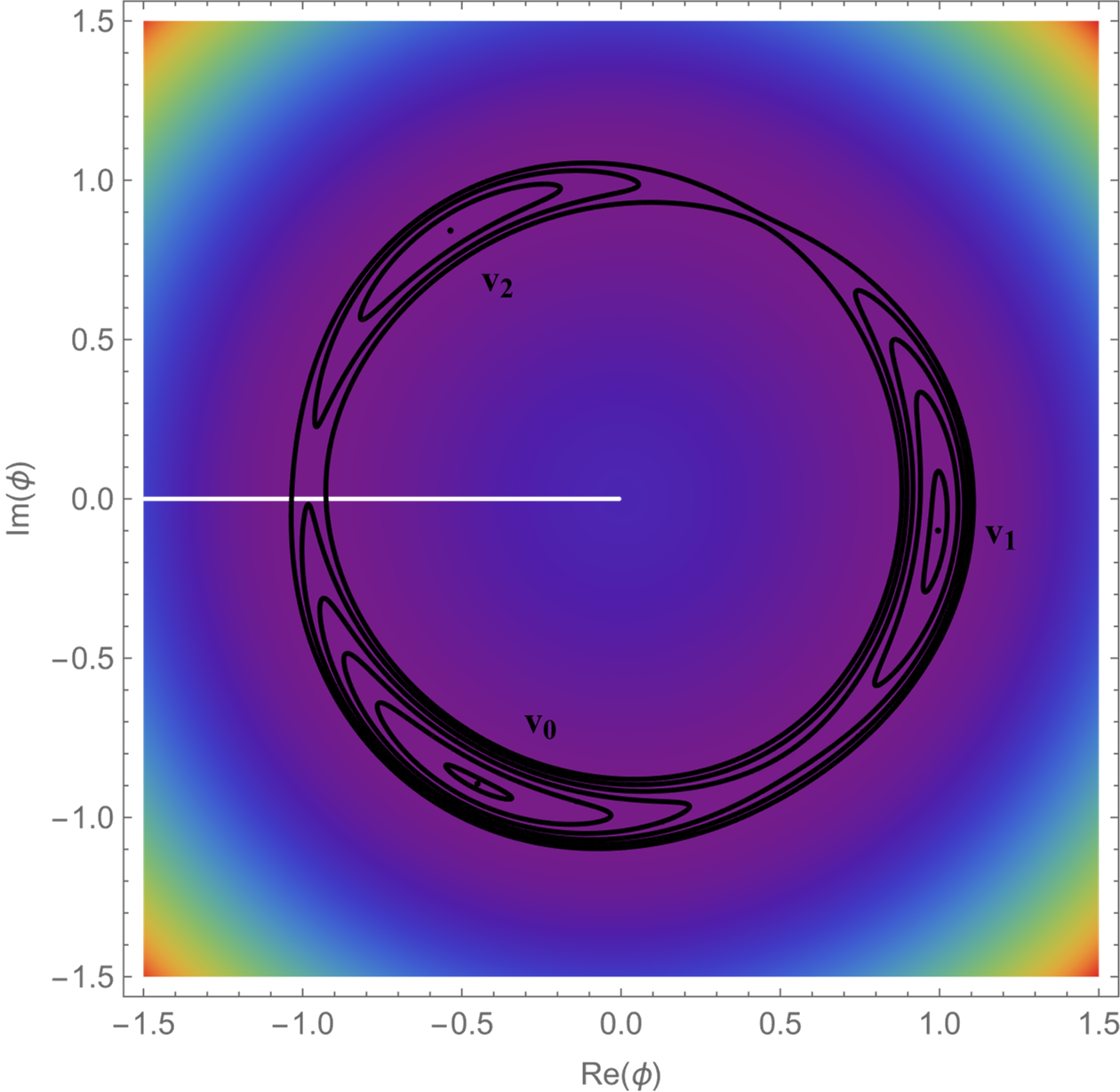
Figure 1: The contour plot of the potential in Eq. (15), with parameters $N=3$, ${m}/(\sqrt{\lambda}\eta)=0.2$, $\Xi_{1}=-0.0005$, and $\Xi_{2}=0.004$. The potential increases progressively in the vacua near the phases $4\pi/3$, 0, and $2\pi/3$, which are labeled as $v_{0}$, $v_{1}$, and $v_{2}$, respectively.

We define $\Delta V$ as the largest potential difference among the three vacua, $\Delta V=\Delta V_{02}$, and introduce the relative potential difference $\zeta={\Delta V_{01}}/{\Delta V_{02}}$ to characterize the relative value of $V_{1}$, as shown in Fig. 2. This reformulation allows the two independent potential differences, $\Delta V_{01}$ and $\Delta V_{02}$, to be expressed in terms of $\Delta V$ and $\zeta$. By varying $\zeta$, we can investigate how bias directions influence the evolutions of domain walls.

Figure 2: Diagram of the energy levels for three non-degenerate vacua, where $V_{0}$ represents the potential values of the true vacuum, while $V_{1}$ and $V_{2}$ correspond to the potential values of the two false vacua. $\Delta V$ denotes the potential difference between the highest-energy vacuum ($V_{2}$) and the true vacuum ($V_{0}$). The ratio $\zeta$ characterizes the relative potential difference between the two false vacua and the true vacuum, defined as $\zeta={\Delta V_{01}}/{\Delta V}$.

The standard evolution of a scalar field is governed by the Klein-Gordon equation,

$$\frac{\partial^{2}\phi}{\partial t^{2}}+3H\frac{\partial\phi}{\partial t}-\nabla^{2}\phi=-\frac{\partial V}{\partial\phi},$$ (10)

where $\nabla^{2}$ is the Laplacian in physical coordinates, and $H$ is the Hubble parameter. An equivalent form is

$$\phi^{\prime\prime}+2\mathcal{H}\phi^{\prime}-\nabla_{\mathbf{x}}^{2}\phi=-a^{2}\frac{\partial V}{\partial\phi},$$ (11)

where a prime denotes the derivative with respect to the conformal time, and $\nabla_{\mathbf{x}}^{2}$ is the Laplacian in the comoving coordinates. This equation implies that the physical thickness of domain walls remains constant throughout their evolution, as derived from $d^{2}\phi/dz^{2}-dV/d\phi=0$. As the Universe evolves, their comoving width $\delta_{c}$ decreases as $\delta_{c}\propto a^{-1}(t)$, where $a(t)$ is the scale factor.

IV Simulation setup

Now we briefly summarize the setup of our numerical simulations. For more details, please refer to Appendices A, B, C and D.

Lattice simulations are performed in a cubic box with $\mathrm{N}^{3}$ grid points and a comoving volume $V=L^{3}$, where $\mathrm{N}$ is the number of grid points along each dimension, $L$ denotes the comoving box size. We use $\mathrm{N}$ in math roman font to distinguish it from the order of symmetry, $N$, used in $Z_{N}$. This box expands with the evolving scale factor $a(t)$, simulating the expansion of the Universe. Without loss of generality, we perform lattice simulations in the radiation-dominated era, where $a\propto\tau$.

Our simulations were performed using the package CosmoLattice, employing the second-order Velocity-Verlet algorithm [53, 54].

IV.1 PRS method

The annihilation times of different domain walls can vary widely depending on bias directions. This variation poses challenges for simulations, as it demands a larger dynamical range to accurately track domain walls behavior and determine their annihilation times.

In simulations, it is essential to maintain the thickness of domain walls several times the spacing of the grid, expressed as $\delta_{c}\geq nL/\mathrm{N}$, where $n$ is a positive integer. However, as domain walls thin in comoving coordinates over time, meeting this requirement becomes increasingly difficult. Moreover, the Hubble horizon must remain smaller than the simulation box size, further constraining the dynamical range.

For instance, in simulations with $\mathrm{N}=512$, the expansion factor $a_{f}/a_{i}$ typically reaches only about a dozen, where $a_{i}$ and $a_{f}$ represent the initial and final scale factors,respectively. However, to accurately study annihilation times, the expansion factor must be on the order of hundreds, which is far beyond what standard methods can achieve.

To overcome these limitations, we employ the Press-Ryden-Spergel (PRS) method [12]. This method maintains a constant comoving domain wall thickness throughout simulations, significantly extending the achievable dynamical range. Additionally, it preserves the tension of domain walls, ensuring that their large-scale dynamics remains consistent with physical expectations. The PRS method has been rigorously validated [12, 55] and widely applied in studies of the evolution of topological defects [56, 57, 58, 59, 60].

In the PRS method, the equation of motion (11) is modified as follows:

$$\phi^{\prime\prime}+\alpha\mathcal{H}\phi^{\prime}-\nabla_{\mathbf{x}}^{2}\phi=-a^{\beta}\frac{\partial V}{\partial\phi}.$$ (12)

To preserve the dynamics of the planar domain walls, $\alpha+\beta/2$ must equal 3 [12]. To maintain the comoving thickness constant, we set $\beta=0$, which implies $\alpha=3$. This simplifies the equation to

$$\phi^{\prime\prime}+3\mathcal{H}\phi^{\prime}-\nabla_{\mathbf{x}}^{2}\phi=-\frac{\partial V}{\partial\phi}.$$ (13)

Our simulations use this modified form, enabling us to achieve the necessary dynamical range while preserving accurate dynamics of domain walls.

IV.2 Redefinition of variables

Our simulation calculations are performed using dimensionless quantities, referred to as program variables. These dimensionless quantities are defined as

$$\tilde{\tau}=\sqrt{\lambda}\eta\tau,\quad\tilde{x}_{i}=\sqrt{\lambda}\eta x_{i},\quad\tilde{\phi}=\frac{\phi}{\eta},$$ (14)

where $\tau$ denotes the physical conformal time, $x_{i}$ represents the comoving distance, and tilded quantities correspond to their program variable counterparts. The program potential is defined as

$$\tilde{V}(\tilde{\phi})\equiv\frac{1}{\lambda\eta^{4}}V(\eta\tilde{\phi})=\frac{1}{4}(|\tilde{\phi}|^{2}-1)^{2}+\left(\frac{m}{\sqrt{\lambda}\eta}\right)^{2}\frac{1}{N^{2}}(1-|\tilde{\phi}|\cos N\theta)+\Xi_{1}\tilde{\phi}_{1}+\Xi_{2}\tilde{\phi_{2}}.$$ (15)

The explicit equations of motion, expressed in terms of program variables, are provided in Appendix A.

V Field configurations and evolution of the area density

First, we verify whether the scaling properties of domain walls hold in our simulations. In addition to the basic parameters listed in Appendix C, we set $\Xi_{1}=\Xi_{2}=0$. We compute the area parameter using the method described in Appendix D. Figure 3 presents the evolution of the area parameters over time in the absence of bias. As observed, once domain walls stabilize, they enter the scaling regime, during which the area parameters for different domain walls remain nearly constant. We perform a constant fit to the total area parameter, $\mathcal{A}_{tot}$, for $\tilde{\tau}>16$ and obtained an approximate value of 2.223 during the scaling stage. Thus, our simulations confirm that the scaling properties of stable domain walls are preserved. We attribute the late-stage increase in the area parameter to numerical errors.

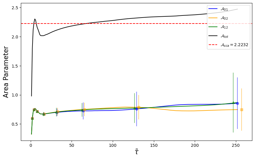
Figure 3: Evolution of the area parameters for each type of domain wall, as well as the total area parameter, with respect to the program time $\tilde{\tau}$, in the absence of bias, $\Xi_{1}=\Xi_{2}=0$.

Next, we observe the evolution of unstable domain walls by setting $\Xi_{2}=0.02$ and $\Xi_{1}=-0.01$. The spatial distribution of the scalar field phase at different program times is shown in slices in Fig. 4. Initially, cosmic strings and domain walls connected to them are formed, separating different domains. Then, Vacuum 2 begins to decay, leaving only Vacuum 0 and Vacuum 1 in our simulated box. After some evolution, Vacuum 1 also begins to decay, and finally, only Vacuum 0 dominates.

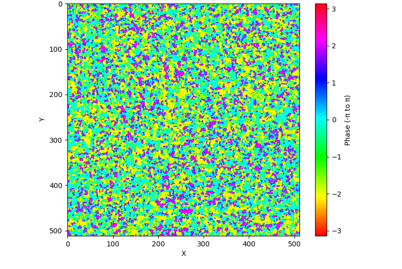
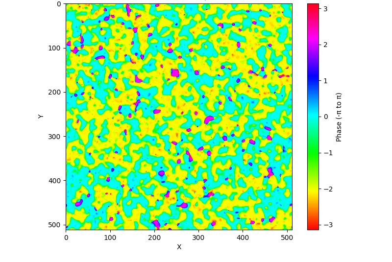
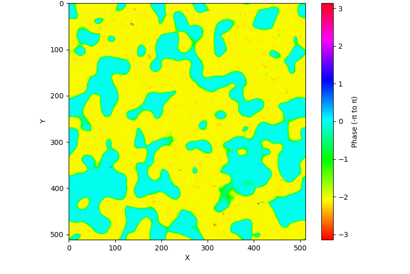
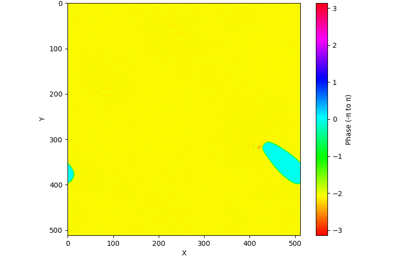
Figure 4: Phase distributions of the field at different moments, with model parameters are $\Xi_{2}=0.02,\Xi_{1}=-0.01$, are shown in slices. Arranged from top left to bottom right, these correspond to program times $\tilde{\tau}$ of 5, 13, 37, and 256, respectively. The phase values are mapped continuously within the range of $-\pi$ to $\pi$, represented by a gradient of colors.

Figure 5 illustrates the evolution of the area of various domain walls over the program time $\tilde{\tau}$ with the parameters set to $\Xi_{1}=-0.01$ and $\Xi_{2}=0.02$, corresponding to $\zeta\approx\ 0.066$. As we can find that the annihilation of domain walls is divided into two stages. In the first stage, the annihilation of the 12-DW and 02-DW occurs simultaneously due to the decay of the Vacuum 2. After the annihilation of these two types of domain walls, only the 01-DW remains. As the system evolves, the 01-DW also annihilates after a certain period.

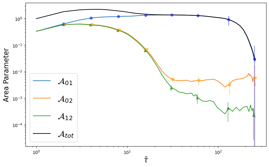
Figure 5: Evolution of the area parameters for each type of domain wall, as well as the total area parameter, with respect to the program time $\tilde{\tau}$, when parameters are set to $\Xi_{1}=-0.01$ and $\Xi_{2}=0.02$.

Additionally, we find that as the 12-DW and 02-DW annihilate, the area of the 01-DW slightly increases. This can be interpreted as a process where the 02-DW and 12-DW “merge” into the 01-DW during the decay of Vacuum 2. Due to this process, the total area decreases more gradually during the first stage of the domain wall annihilation.

We notice that, near the moment of annihilation of domain walls, the area of domain walls oscillates due to field fluctuations. Therefore, we need to reconsider our estimation of the annihilation time, rather than simply using the moment when the area parameter reaches zero as the annihilation time. For this reason, we define the annihilation time of each type of domain walls as the time when the area parameter first drops below 0.01. This corresponds to the level where the area parameter is approximately 1% of its value during the scaling regime.

VI Estimation of the annihilation time

The fixed parameters listed in Appendix C are used in our simulations, and we set $\Xi_{2}=0.02$ which results in $\delta\tilde{V}\approx\sqrt{3}\Xi_{2}=0.0342$), while $\Xi_{1}$ and the corresponding $\zeta$ values are selected as listed in Table 1.

$\quad\Xi_{1}\quad$	$-0.01$	$-0.008$	$-0.007$	$-0.006$	$-0.004$	$-0.002$	0	0.002	0.004	0.006	0.01
$\quad\zeta\quad$	0.0067	0.153	0.196	0.239	0.325	0.411	0.498	0.584	0.671	0.758	0.933

Table 1: Values of $\Xi_{1}$ and $\zeta$ used in simulations.

Using the method for measuring the annihilation time proposed at the end of Sec. V, we determined the dependence of the annihilation time of various domain walls on $\zeta$, as shown in Fig. 6.

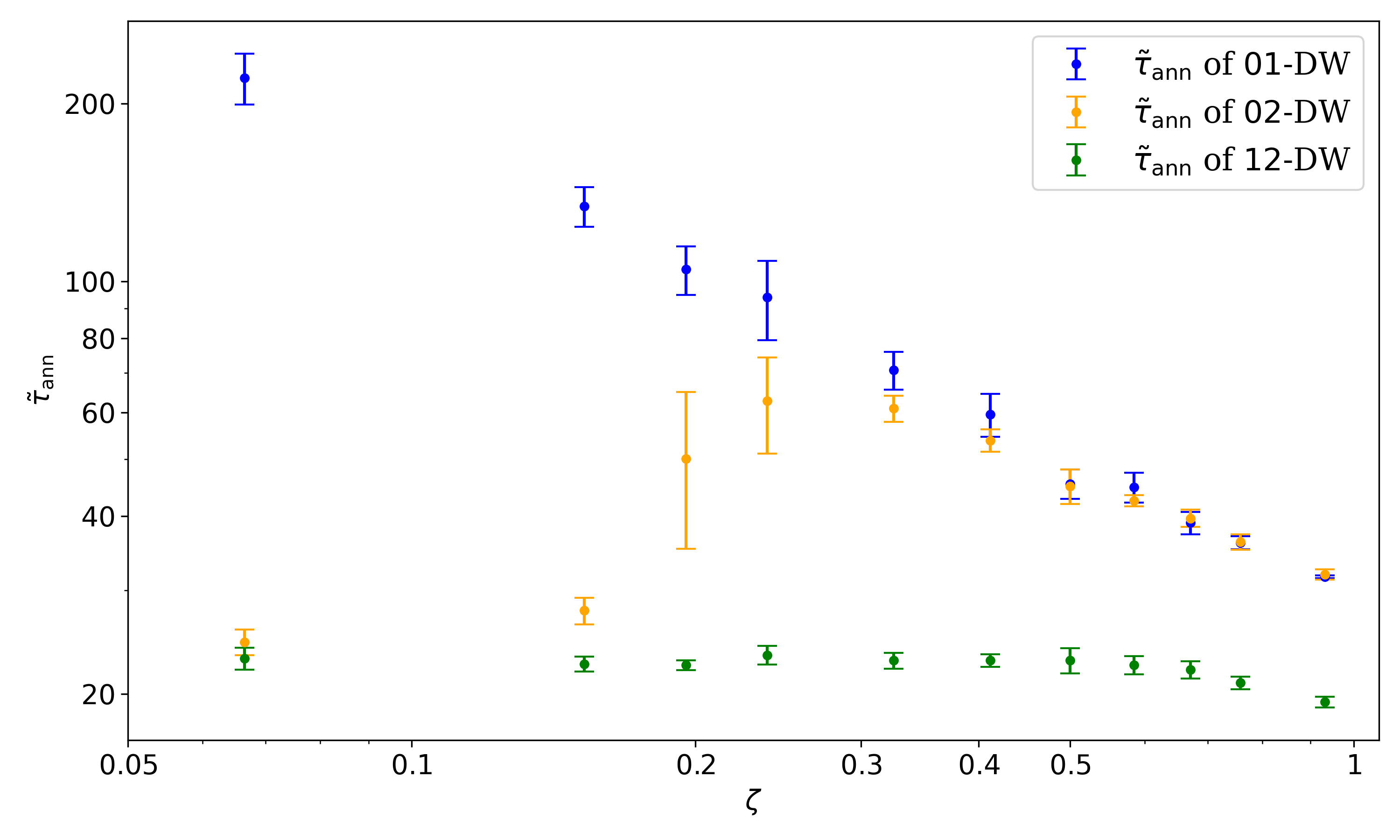
Figure 6: Dependence of the annihilation time (in program units) of various domain walls on the parameter $\zeta$.

Based on the simulation results, we now attempt to provide a semi-analytical expression for the annihilation time of various domain walls. First, for the 01-DW, in the late stages of evolution, since only Vacuum 0 and Vacuum 1 remain in the Universe, the behavior of the 01-DW becomes similar to that of the $Z_{2}$ domain walls. Therefore, we estimate the annihilation time of the 01-DW in the same way as the annihilation time of the $Z_{2}$ domain walls,

$$t_{\text{ann},01}\sim\frac{\sigma}{\Delta V_{01}}=\frac{8m\eta^{2}}{9\zeta\Delta V}.$$ (16)

From this we obtain

$$\tilde{\tau}_{\text{ann},01}=\kappa\left(\frac{m}{\sqrt{\lambda}\eta}\right)^{1/2}\left(\zeta\Delta\tilde{V}\right)^{-1/2},$$ (17)

the numerical factor $\kappa$ is obtained by fitting the simulation results. From Fig. 7, the best-fit value for the numerical coefficient $\kappa$ is found to be

$$\kappa=7.24.$$ (18)

From Eqs. (17) and (18), we obtain the expression for the annihilation time of the 01-DW,

$$t_{\text{ann},01}\approx 26.2\frac{m\eta^{2}}{\zeta\Delta V}.$$ (19)

This dependence is consistent with the conclusions of previous studies [29, 6].

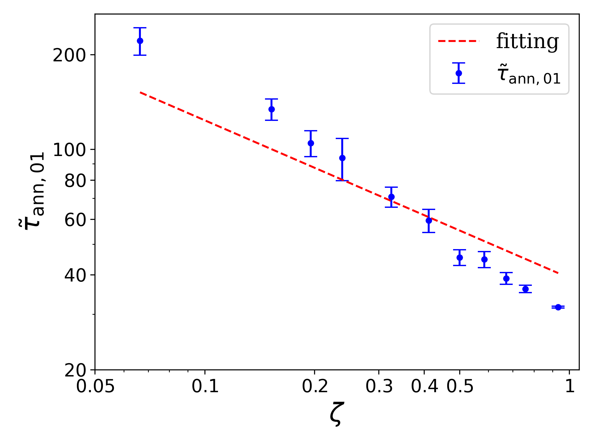
Figure 7: Annihilation time of the 01-DW, $\tilde{\tau}_{\text{ann},01}$, as a function of the potential difference ratio $\zeta$. The red dashed line represents the fit given by Eq. (17).

The annihilation time of the 12-DW is essentially unaffected by bias directions. For small values of $\zeta$, $\Delta V_{01}$ is rather small. As the vacuum bubbles of Vacuum 2 collapse, the 12-DW and the 02-DW annihilate almost simultaneously, as shown in Fig. 5.

For larger values of $\zeta$, $\Delta V_{12}$ becomes smaller. As both Vacuum 1 and Vacuum 2 decay into Vacuum 0, the size of the vacuum bubbles of Vacuum 1 and Vacuum 2 shrink below the Hubble horizon. At this stage, the 12-DW separating the two vacua forms a finite-sized, closed string boundary. Due to the string tension, this boundary rapidly contracts, causing the 12-DW to annihilate quickly. As a result, the two vacuum bubbles on either side separate into distinct individual bubbles. In Fig. 8, the red bubble near $x=400,y=80$ separating from the cyan bubble serves as an example of this process.

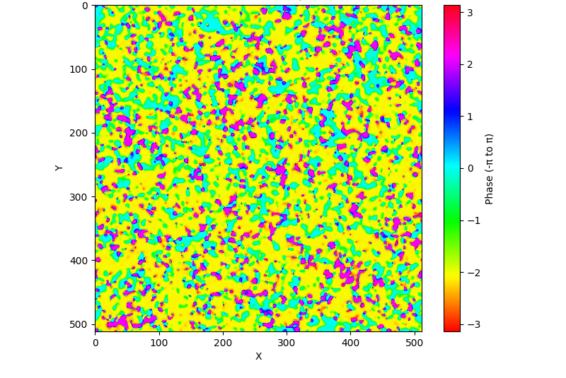
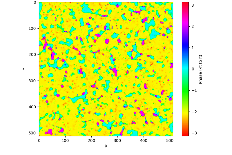
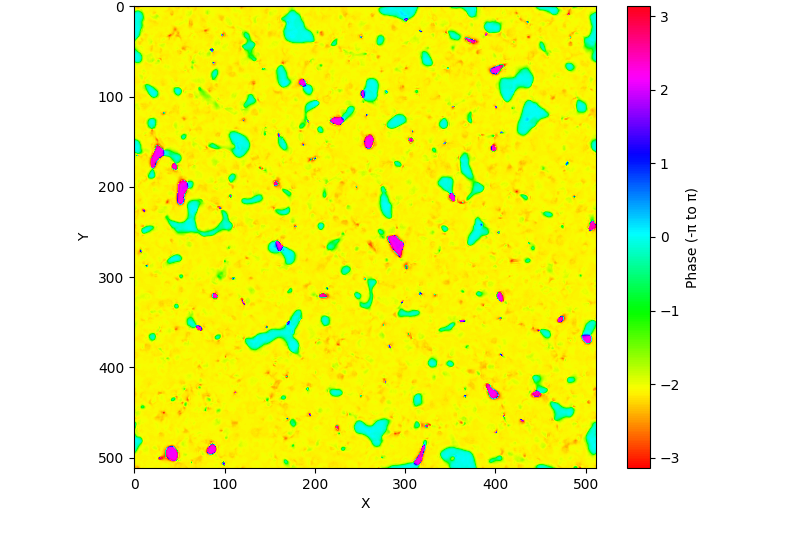
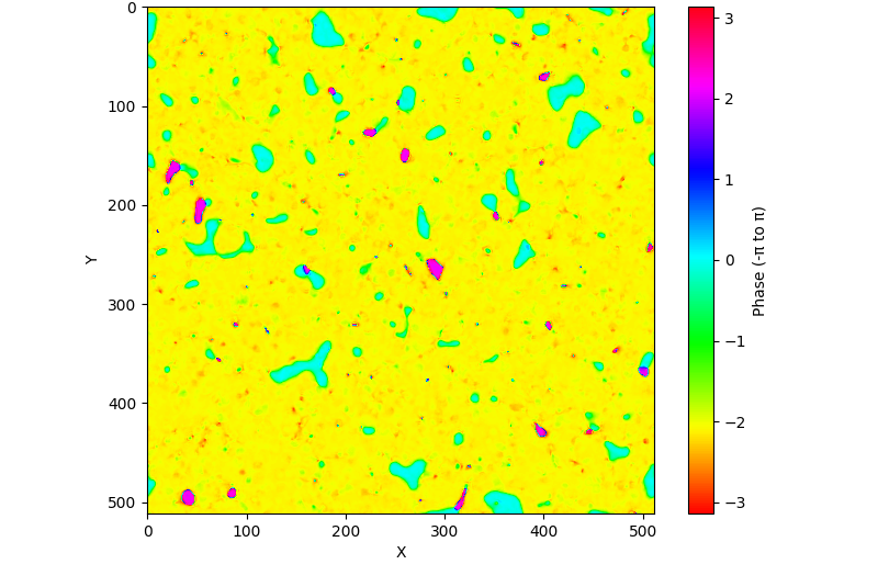
Figure 8: Phase distribution of the field at different moments for model parameters $\Xi_{2}=0.02,\Xi_{1}=0.004$, shown in slices. Arranged from top left to bottom right, these correspond to program times $\tilde{\tau}$ of 9, 14, 19, and 20, respectively. The phase values are continuously mapped within the range of $-\pi$ to $\pi$, represented using a gradient of colors.

Therefore, for small $\zeta$, the annihilation of the 12-DW is mainly driven by the pressure difference on either side of domain walls, whereas for large $\zeta$, it is predominantly governed by the tension of the closed string. According to Fig. 6, as $\zeta$ approaches 1, the annihilation times of the 12-DW and the 01-DW become early identical. Thus, we estimate the annihilation time of the 12-DW, using the value of $t_{\text{ann},01}$ at $\zeta=1$,

$$t_{\text{ann},12}\approx 26.2\frac{m\eta^{2}}{\Delta V}.$$ (20)

The annihilation of the 12-DW has not been explicitly discussed in previous studies.

The dependence of the annihilation time of 02-DW $\tilde{\tau}_{\text{ann},02}$ on $\zeta$ can be analyzed in two regimes. For $\zeta<0.3$, the annihilation time increases with $\zeta$. This can be understood as follows: as the energy of Vacuum 1 increases, the potential difference between Vacuum 2 and Vacuum 1 decreases, leading to a slower decay rate from Vacuum 2 to Vacuum 1. As a result, the decay time of Vacuum 2 increases. For $\zeta>0.3$, the decay rate from Vacuum 1 to Vacuum 0 becomes sufficiently large, allowing Vacuum 0 to quickly dominates. After this, the remaining two vacua almost decay synchronously.

For $\zeta<0.3$, we can simply perform a linear fit to the relationship between $\tilde{\tau}_{02}$ and $\zeta$, as shown in Fig. 9,

$$\tilde{\tau}_{\text{ann},02}\approx (56.3\zeta+7.24)\left(\frac{m}{\sqrt{\lambda}\eta}\right)^{1/2}\Delta\tilde{V}^{-1/2},\quad\zeta\leq 0.3.$$ (21)

Alternatively, this can be expressed in terms of the cosmic time,

$$t_{\text{ann},02}\approx(56.3\zeta+7.24)^{2}\frac{m\eta^{2}}{\Delta V},\quad\zeta\leq 0.3.$$ (22)

For $\zeta>0.3$, we can estimate $\tilde{\tau}_{\text{ann},02}$ using $\tilde{\tau}_{\text{ann},01}$,

$$t_{\text{ann},02}\approx 26.2\frac{m\eta^{2}}{\zeta\Delta V},\quad\zeta>0.3.$$ (23)

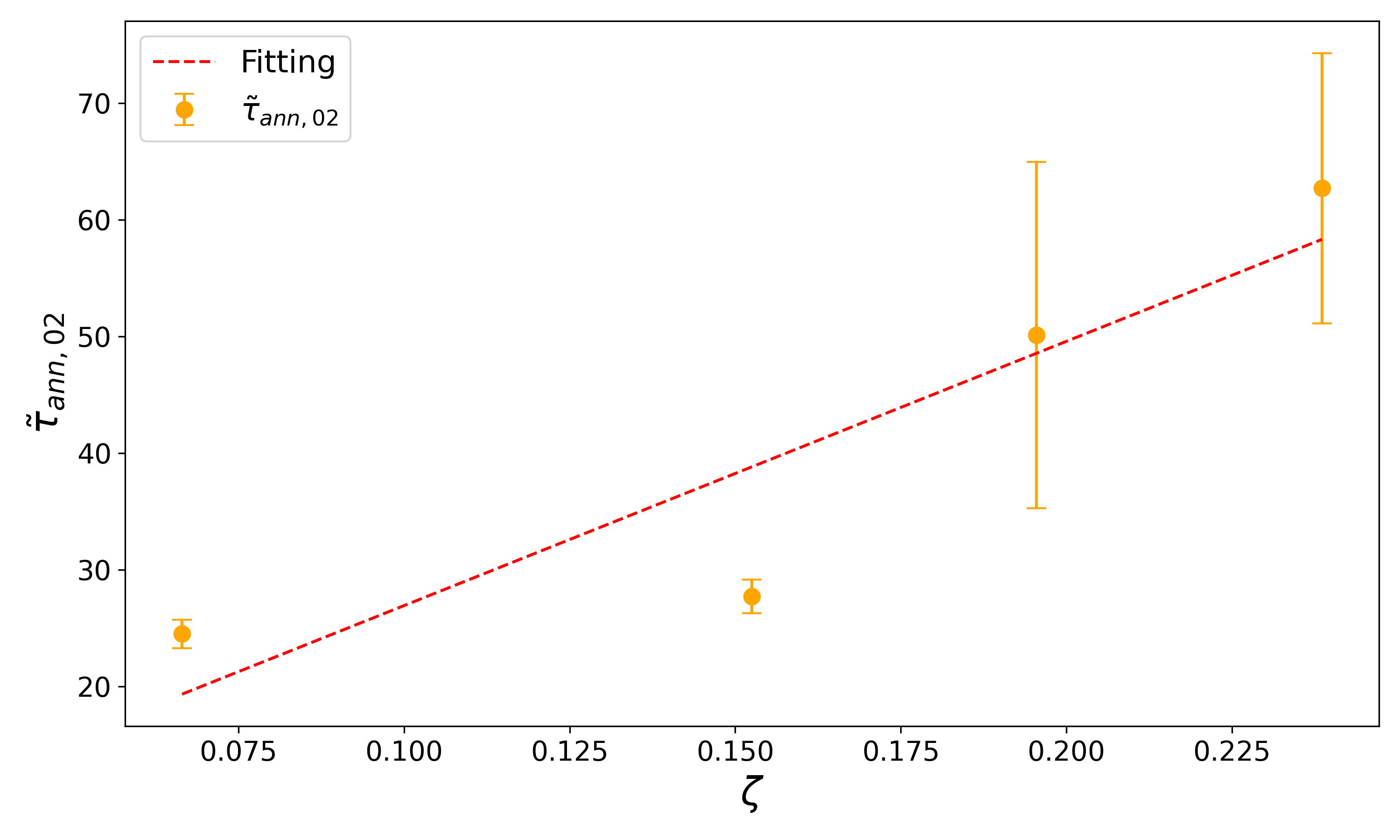
Figure 9: Dependence of annihilation time of the 02-DW, $\tilde{\tau}_{\text{ann},02}$ on $\zeta$, for $\zeta<0.3$ for $\Xi_{2}=0.02$ where $\zeta$ is less than 0.3.

In addition, to minimize errors in estimating the annihilation time of the 02-DW due to its rapid annihilation, we also examined the dependence of $\tilde{\tau}_{\text{ann},02}$ on $\zeta$ for smaller $\Xi$. The results are shown in Appendix E.

In previous research, the relationship between the annihilation time of the 02-DW and bias directions has been rarely explored. Researchers have often estimated the annihilation time of this type of domain walls using methods similar to those for $Z_{2}$ domain walls. However, our simulation results indicate that the annihilation time of the 02-DW is not solely determined by the potential difference between Vacuum 2 and the true vacuum; rather, it also exhibits a nontrivial dependence on bias directions.

VII Summary and discussion

In this study, we have investigated the impact of bias directions on the dynamics of $Z_{N}$ domain walls, with a particular focus on quantitatively describing the evolution of domain walls by estimating their annihilation times. We set $N=3$ to examine the dynamics of domain walls in a $Z_{3}$ symmetric system and analyzed how strings and domain walls arise. To avoid the domain wall problem, we introduced bias terms into the potential. In addition, we used $\Delta V$ to quantify the magnitudes of the biases and $\zeta$ to characterize their directions.

We numerically investigate the nonlinear dynamics of domain walls in a radiation-dominated Universe where lattice simulations are performed in a cubic box. We employed dimensionless quantities in our calculations to ensure the results are general. Simulations explored the domain wall evolution under various bias configurations, controlled by the parameters $\Xi_{1}$ and $\Xi_{2}$, and examined their effects on annihilation times.

Based on our simulation results, we have derived analytical expressions for annihilation times of domain walls. For the 01-DW, the annihilation time $t_{\text{ann},01}$ depends inversely on $\zeta$, following $t_{\text{ann},01}\sim\sigma/(\zeta\Delta V)$. For the 12-DW,the annihilation time is roughly unaffected by bias directions, estimated as $t_{\text{ann},12}\sim\sigma/\Delta V$. The annihilation time of the 02-DW exhibits a more intricate dependence on both the potential difference and bias directions. For $\zeta<0.3$, $t_{\text{ann},02}$ increases linearly with $\zeta$, while for $\zeta>0.3$, it aligns with the behavior of the 01-DW. More detailed estimations are given by Eqs. (19), (20), and (23).

The estimate of $t_{\text{ann},01}$ is consistent with previous results [29, 6]. The annihilation time of domain walls between the false vacua, such as $t_{\text{ann},12}$, has not been systematically investigated in previous studies. The estimate of $t_{\text{ann},02}$ corrects the previous simple assumption that it is independent of bias directions [33].

Although our study primarily focuses on the evolution and dynamics of $Z_{3}$ domain walls, the characterization of bias directions in this work can also be generalized to the $N>3$ cases. Further investigations can be conducted. We predict that for $N>3$, the dynamics of domain walls will become more complex, involving more independent parameters.

Stepwise annihilation of domain walls is expected to produce double-peak or multi-peak structures of the GW energy spectrum [33], leading to more distinguishable observational GW signals arising from $Z_{N}$ domain walls compared to single-peak structures. The peak amplitude and frequency of the GW spectrum generated by domain walls depend on their annihilation time [61, 62, 63]. Therefore, our estimate of the domain wall annihilation times can improve the accuracy of predictions for the GW spectrum arising from $Z_{N}$ domain walls.

Additionally, we observe the remaining domain wall area temporarily increases due to the stepwise annihilation of domain walls. Consequently, the reduction in the total area parameter during each stage of the domain wall annihilation is not uniform. By fully considering this effect, we may achieve more precise estimations of the GW spectrum produced by domain walls. Furthermore, we anticipate that future studies could directly simulate the GW spectrum to examine or reveal the dependence of its spectral shape on bias directions. Such simulations could also provide an opportunity to observe double-peak or multi-peak structures in the GW spectrum arising from $Z_{N}$ domain walls.

Appendix A Equations of Motion

In our simulations, we define two real fields to represent a complex scalar field, $\tilde{\phi}=\tilde{\phi}_{1}+i\tilde{\phi}_{2}$. Based on Eqs. (13) and (15), the equations of motion for the real scalar fields are given as follows:

$$\tilde{\phi}_{1}^{\prime\prime}+3\frac{a^{\prime}}{a}\tilde{\phi}_{1}^{\prime}-\nabla^{2}\tilde{\phi}_{1} =-\Xi_{1}-\tilde{\phi}_{{1}}\left(-1+\tilde{\phi}_{\mathbf{1}}^{2}+\tilde{\phi}_{2}^{2}\right)+\frac{m^{2}}{{N^{2}\sqrt{\tilde{\phi}_{1}^{2}+\tilde{\phi}_{2}^{2}}}}\left[\cos\left(N\theta\right)\tilde{\phi}_{1}+N\sin\left(N\theta\right)\tilde{\phi}_{2}\right],$$ (24)

$$\tilde{\phi}_{2}^{\prime\prime}+3\frac{a^{\prime}}{a}\tilde{\phi}_{2}^{\prime}-\nabla^{2}\tilde{\phi}_{2} =-\Xi_{2}-\tilde{\phi}_{{2}}\left(-1+\tilde{\phi}_{\mathbf{1}}^{2}+\tilde{\phi}_{2}^{2}\right)-\frac{m^{2}}{{N^{2}\sqrt{\tilde{\phi}_{1}^{2}+\tilde{\phi}_{2}^{2}}}}\left[\cos\left(N\theta\right)\tilde{\phi}_{2}+N\sin\left(N\theta\right)\tilde{\phi}_{1}\right].$$ (25)

Here, a prime denotes differentiation with respect to the program time, and $\nabla^{2}$ represents the Laplacian operator with respect to the program coordinates.

Appendix B Initial Conditions

The scale factor can be expressed in terms of the dimensionless conformal time as

$$a(\tilde{\tau})=\frac{\sqrt{\lambda}\eta}{H_{i}}\frac{\tilde{\tau}}{\tilde{\tau}_{i}^{2}},$$ (26)

where $H_{i}$ is the initial Hubble parameter. By convention, we set the initial scale factor $a(\tilde{\tau_{i}})$ to unity,

$$a(\tilde{\tau}_{i})=1.$$ (27)

Although the initial time in simulations is arbitrary, we choose

$$H_{i}=\sqrt{\lambda}\eta,$$ (28)

which simplifies the initial dimensionless conformal time to

$$\tilde{\tau}_{i}=1.$$ (29)

Thus, we derive the simple relation,

$$\tilde{\mathcal{H}}_{i}^{-1}(\tilde{\tau})=a({\tilde{\tau}})=\tilde{\tau},$$ (30)

where $\tilde{\mathcal{H}}$ denotes the dimensionless comoving Hubble parameter, and $\tilde{\mathcal{H}}_{i}^{-1}$ represents the dimensionless comoving Hubble horizon.

Since the late stage evolution of domain walls is largely independent of the initial conditions [64], we adopt a Gaussian distribution for simplicity. The initial mean values of the scalar field $\tilde{\phi}_{i}$ and its time derivative $\tilde{\phi}^{\prime}_{i}$ are set to zero, while their perturbations are characterized in momentum space by the correlation functions,

$$\langle\tilde{\phi}_{i}(\mathbf{k})\tilde{\phi}_{i}(\mathbf{k}^{\prime})\rangle =\frac{1}{2k}(2\pi)^{3}\delta^{(3)}(\mathbf{k}+\mathbf{k}^{\prime}),$$ (31)

$$\langle\tilde{\phi}^{\prime}_{i}(\mathbf{k})\tilde{\phi}^{\prime}_{i}(\mathbf{k}^{\prime})\rangle =\frac{k}{2}(2\pi)^{3}\delta^{(3)}(\mathbf{k}+\mathbf{k}^{\prime}),\quad(i=1,2).$$ (32)

Here, $\tilde{\phi}^{\prime}$ represents the time derivative of the scalar field in simulations, $\mathbf{k}^{\prime}$ refers to modes distinct from $\mathbf{k}$, and $k$ represents the magnitude of $\mathbf{k}$. Since the effective mass of the scalar field is initially negative, we approximate the field as massless by replacing $\sqrt{k^{2}+m^{2}}$ with $k$.

To suppress unphysical noise from high-frequency modes, we introduce a momentum cutoff $k_{\text{cut}}$. Fluctuations are set to zero for all modes with $k>k_{\text{cut}}$. In our setup, we set the cutoff value to $\tilde{k}_{\text{cut}}=3$.

Appendix C Parameters for simulations

Since simulations are performed with dimensionless quantities, the simulation results are independent of the specific values of the dimensionless coefficients. This allows us to set these parameters arbitrarily. We set $\lambda=0.1$ and $\eta=2\times 10^{17}\,\text{GeV}$. Additionally, We choose $m=\sqrt{\lambda}\eta$ for clarity.

Simulating topological defects presents two primary challenges: i) To ensure resolvability, the defect thickness must be larger than $L/\mathrm{N}$, the ultraviolet limit.ii) The Hubble horizon must remain smaller than the box size, defining the infrared limit.

The physical thicknesses are given by $\delta_{s}\approx(\sqrt{\lambda}\eta)^{-1}$ for strings and $\delta_{w}\approx m^{-1}$ for domain walls [2]. In the PRS method, those correspond to the comoving thicknesses, $\delta_{s,c}\approx(\sqrt{\lambda}\eta)^{-1}$ and $\delta_{w,c}\approx m^{-1}$. The ratio of the two thicknesses is $\delta_{s}/\delta_{w}\approx m/(\sqrt{\lambda}\eta)$. For the parameters we selected, $\delta_{w}\approx\delta_{s}$. We choose $\delta_{s(w),c}\approx L/\mathrm{N}$, or equivalently, in terms of mensionless quantities

$$\tilde{\delta}_{s(w),c}\approx\tilde{L}/\mathrm{N}.$$ (33)

This resolution marginally meets the requirement.

Another constraint comes from the requirement that the Hubble horizon at the end of simulations must remain within the box size, $H_{f}^{-1}\leq a_{f}L$, or equivalently, $\mathcal{H}_{f}^{-1}\leq L$, to ensure that the evolution is not influenced by boundary conditions. In terms of program variables, this condition becomes:

$$\tilde{\mathcal{H}}_{f}^{-1}=\tilde{\tau}_{f}\leq\tilde{L}.$$ (34)

In our simulations, $\mathrm{N}$ is set to 512. Based on Eq. (33), we choose $\tilde{L}=512$. Our simulations ends when the Hubble horizon reaches half the size of the comoving box, $\tilde{\tau}_{f}=\tilde{\mathcal{H}}_{f}^{-1}=256$.

Appendix D Calculation of the Area Parameter

We adopt the method described in [65, 38] to measure the comoving area of domain walls. Unlike previous studies, which computed the comoving area and area parameters by considering all domain wall types collectively, we aim to examine the evolution of each specific type of domain walls separately. Below, we outline the method used to compute the area of domain walls.

First, we divide the field values into three regions based on the phase of the saddle points in the potential function in Eq. (III) (for the case of $\Xi=0$, these phases are $\pi/3,\pi,5\pi/3$). Each region contains a vacuum state and is labeled by its corresponding vacuum number. After extracting the phase for each field point at every output snapshot, we assign labels based on the corresponding field value range. See Fig. 10 as an example. Hereafter, we refer to the field values within each region $i$ as Vacuum $i$.

Figure 10: An example of phase separation, with the potential barrier as the boundary, in the case where $\Xi_{1}=0$ and $\Xi_{2}=0$.

Next, for each field point, we compare the labels of neighboring points. If the labels of two points differ, say label $i$ and label $j$, we increment $N_{ij}$ by one, where $N_{ij}$ represents the count of the domain wall area elements corresponding to the $ij$-DW. This comparison is conducted along the three coordinate axes. Specifically, each grid point $(x,y,z)$ is compared with its neighbors $(x+1,y,z)$, $(x,y+1,z)$, and $(x,y,z+1)$. This procedure is applied across all grid points at each time step to determine the area count for each type of domain wall. An example of identifying a domain wall in two dimensions is presented in Fig. 11.

Figure 11: An example of identifying a domain wall in two dimensions is shown. The point $(x,y)$ is labeled as Vacuum $i$, while its two adjacent points in directions of increasing coordinates are labeled as Vacuum $j$. From this, we infer that a domain wall spans between $(x,y)$ and its two neighboring points. Thus, we represent the area of domain walls as the line segment connecting $(x,y)$ and its two adjacent points. However, this approach overestimates the domain wall’s area. To obtain the correct comoving area of domain walls, a factor of $2/3$ must be applied.

As noted in [65], direct calculation of the domain wall area using grid points overestimates the actual comoving area. Therefore, considering the random orientations of domain walls, we introduce a correction factor of $2/3$. Hence, the comoving area of each type of domain walls is estimated as:

$$A_{ij}(t)=\frac{2}{3}N_{ij}(t)\times\Delta x^{2},$$ (35)

where $\Delta x\equiv L/\mathrm{N}$ is the comoving lattice spacing. The area parameter is then estimated as:

$$\mathcal{A}_{ij}=\frac{A_{ij}(t)\tau}{V}=\frac{2}{3}\frac{N_{ij}(t)\tau}{\Delta x}.$$ (36)

In [4, 32], the method for calculating the area of domain walls is expressed as:

$$A/V=C\sum_{\mathrm{links}}\delta\frac{|\nabla\theta|}{|\theta_{,x}|+|\theta_{,y}|+|\theta_{,z}|},$$ (37)

where $\delta$ takes the value of 1 at grid points adjacent to domain walls and 0 elsewhere. The constant $C$ is determined such that $A/V=1$. Our estimation of the domain wall area aligns with this approach in that it averages over different domain wall orientations. However, our method distinguishes between different types of domain walls, providing an additional level of differentiation.

Appendix E Examining the Estimate of $t_{\text{ann,02}}$ for Smaller $\Xi$

We examine the dependence of $\tilde{\tau}_{\text{ann},02}$ on $\zeta$ in the case of $\Xi_{2}=0.006$. Under these conditions, the decay of Vacuum 1 may not necessarily occur within simulations, which does not affect our estimate of $\tilde{\tau}_{\text{ann},02}$, as Figure 12 illustrates.

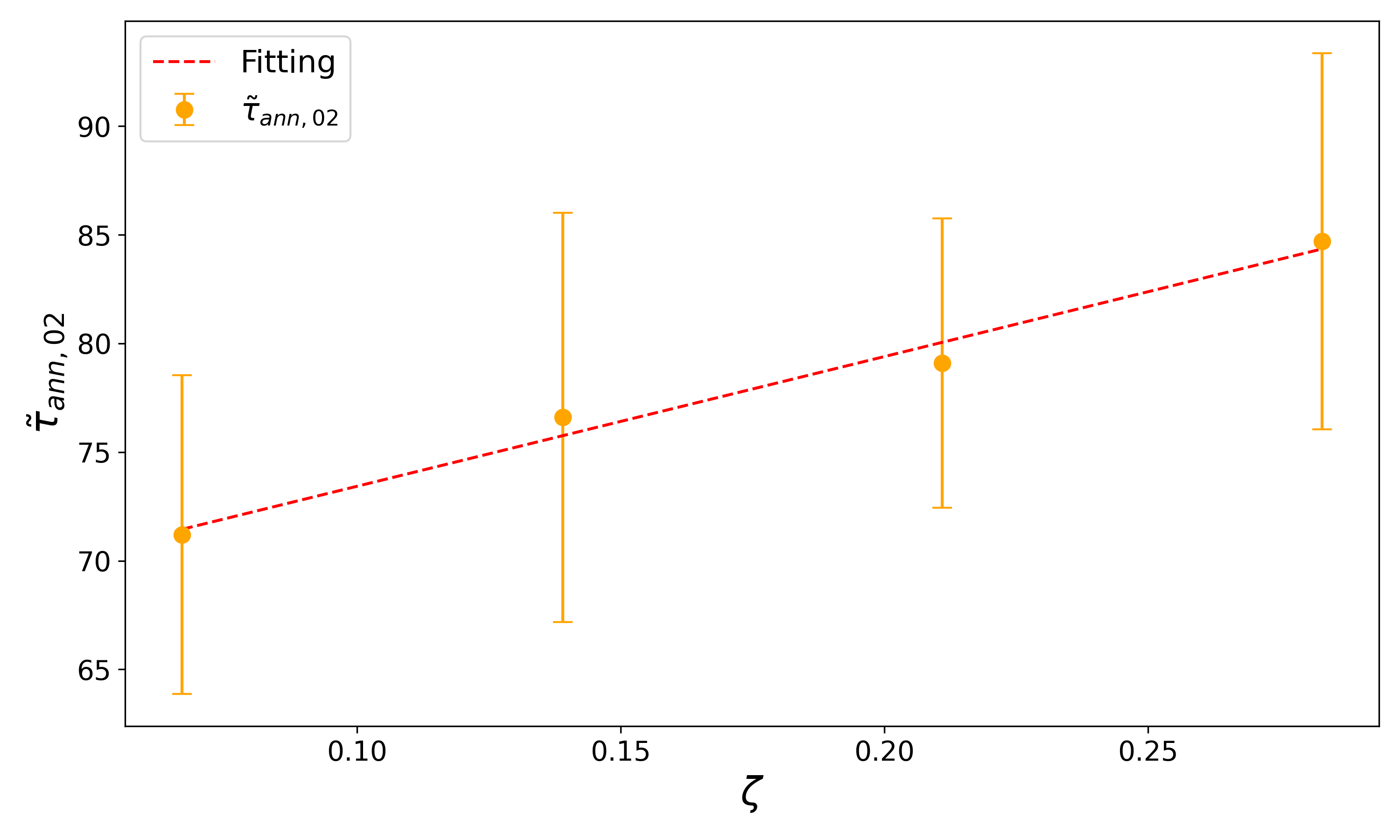
Figure 12: Dependence of the annihilation time of the 02-DW, $\tilde{\tau}_{\text{ann},02}$, on $\zeta$ for $\zeta<0.3$ and $\Xi_{2}=0.006$.

$\tilde{\tau}_{\text{ann},02}$ is consistently above 70, indicating that the system has remained in the scaling regime for a sufficiently long duration. For $\zeta<0.3$, a linear fit describes the data well.

References

- Kibble [1976] T. W. B. Kibble, Topology of Cosmic Domains and Strings, J. Phys. A 9, 1387 (1976).
- Vilenkin and Shellard [2000] A. Vilenkin and E. P. S. Shellard, Cosmic Strings and Other Topological Defects (Cambridge University Press, 2000).
- Saikawa [2017] K. Saikawa, A review of gravitational waves from cosmic domain walls, Universe 3, 40 (2017), arXiv:1703.02576 [hep-ph] .
- Hiramatsu et al. [2010] T. Hiramatsu, M. Kawasaki, and K. Saikawa, Gravitational Waves from Collapsing Domain Walls, JCAP 05, 032, arXiv:1002.1555 [astro-ph.CO] .
- Sikivie [1982] P. Sikivie, Of Axions, Domain Walls and the Early Universe, Phys. Rev. Lett. 48, 1156 (1982).
- Kawasaki et al. [2015a] M. Kawasaki, K. Saikawa, and T. Sekiguchi, Axion dark matter from topological defects, Physical Review D 91, 10.1103/PhysRevD.91.065014 (2015a).
- Marsh [2016] D. J. E. Marsh, Axion Cosmology, Phys. Rept. 643, 1 (2016), arXiv:1510.07633 [astro-ph.CO] .
- Linde [1994] A. D. Linde, Hybrid inflation, Phys. Rev. D 49, 748 (1994), arXiv:astro-ph/9307002 .
- King [2017] S. F. King, Unified Models of Neutrinos, Flavour and CP Violation, Prog. Part. Nucl. Phys. 94, 217 (2017), arXiv:1701.04413 [hep-ph] .
- Xing [2020] Z.-z. Xing, Flavor structures of charged fermions and massive neutrinos, Phys. Rept. 854, 1 (2020), arXiv:1909.09610 [hep-ph] .
- Ibanez and Ross [1992] L. E. Ibanez and G. G. Ross, Discrete gauge symmetries and the origin of baryon and lepton number conservation in supersymmetric versions of the standard model, Nucl. Phys. B 368, 3 (1992).
- Press et al. [1989] W. H. Press, B. S. Ryden, and D. N. Spergel, Dynamical Evolution of Domain Walls in an Expanding Universe, Astrophys. J. 347, 590 (1989).
- Garagounis and Hindmarsh [2003a] T. Garagounis and M. Hindmarsh, Scaling in numerical simulations of domain walls, Phys. Rev. D 68, 103506 (2003a), arXiv:hep-ph/0212359 .
- Oliveira et al. [2005a] J. C. R. E. Oliveira, C. J. A. P. Martins, and P. P. Avelino, The Cosmological evolution of domain wall networks, Phys. Rev. D 71, 083509 (2005a), arXiv:hep-ph/0410356 .
- Avelino et al. [2005a] P. P. Avelino, C. J. A. P. Martins, and J. C. R. E. Oliveira, One-scale model for domain wall network evolution, Phys. Rev. D 72, 083506 (2005a), arXiv:hep-ph/0507272 .
- Oliveira and Martins [2015] M. F. Oliveira and C. J. A. P. Martins, Scaling properties of multitension domain wall networks, Phys. Rev. D 91, 043527 (2015), arXiv:1503.00234 [hep-ph] .
- Leite et al. [2013] A. M. M. Leite, C. J. A. P. Martins, and E. P. S. Shellard, Accurate Calibration of the Velocity-dependent One-scale Model for Domain Walls, Phys. Lett. B 718, 740 (2013), arXiv:1206.6043 [hep-ph] .
- Martins et al. [2016] C. J. A. P. Martins, I. Y. Rybak, A. Avgoustidis, and E. P. S. Shellard, Extending the velocity-dependent one-scale model for domain walls, Phys. Rev. D 93, 043534 (2016), arXiv:1602.01322 [hep-ph] .
- Zel’dovich et al. [1974] Y. B. Zel’dovich, I. Y. Kobzarev, and L. B. Okun, Cosmological consequences of spontaneous violation of discrete symmetry, Zh. Eksp. Teor. Fiz. 40, 3 (1974).
- Srivastava [1999] A. M. Srivastava, Topological defects in cosmology, Pramana 53, 1069 (1999).
- Larsson et al. [1997] S. E. Larsson, S. Sarkar, and P. L. White, Evading the cosmological domain wall problem, Phys. Rev. D 55, 5129 (1997), arXiv:hep-ph/9608319 .
- Gelmini et al. [1989] G. B. Gelmini, M. Gleiser, and E. W. Kolb, Cosmology of Biased Discrete Symmetry Breaking, Phys. Rev. D 39, 1558 (1989).
- Vilenkin [1981] A. Vilenkin, Gravitational Field of Vacuum Domain Walls and Strings, Phys. Rev. D 23, 852 (1981).
- Kamionkowski and March-Russell [1992] M. Kamionkowski and J. March-Russell, Planck scale physics and the Peccei-Quinn mechanism, Phys. Lett. B 282, 137 (1992), arXiv:hep-th/9202003 .
- Holman et al. [1992] R. Holman, S. D. H. Hsu, T. W. Kephart, E. W. Kolb, R. Watkins, and L. M. Widrow, Solutions to the strong CP problem in a world with gravity, Phys. Lett. B 282, 132 (1992), arXiv:hep-ph/9203206 .
- Dobrescu [1997] B. A. Dobrescu, The Strong CP problem versus Planck scale physics, Phys. Rev. D 55, 5826 (1997), arXiv:hep-ph/9609221 .
- Barr and Seckel [1992] S. M. Barr and D. Seckel, Planck scale corrections to axion models, Phys. Rev. D 46, 539 (1992).
- Dine [1992] M. Dine, Problems of naturalness: Some lessons from string theory, in Conference on Topics in Quantum Gravity (1992) arXiv:hep-th/9207045 .
- Hiramatsu et al. [2011] T. Hiramatsu, M. Kawasaki, and K. Saikawa, Evolution of String-Wall Networks and Axionic Domain Wall Problem, JCAP 08, 030, arXiv:1012.4558 [astro-ph.CO] .
- Hiramatsu et al. [2013a] T. Hiramatsu, M. Kawasaki, K. Saikawa, and T. Sekiguchi, Axion cosmology with long-lived domain walls, JCAP 01, 001, arXiv:1207.3166 [hep-ph] .
- Kawasaki et al. [2013] M. Kawasaki, T. T. Yanagida, and K. Yoshino, Domain wall and isocurvature perturbation problems in axion models, JCAP 11, 030, arXiv:1305.5338 [hep-ph] .
- Li, Yang and Bian, Ligong and Cai, Rong-Gen and Shu, Jing [2023] Li, Yang and Bian, Ligong and Cai, Rong-Gen and Shu, Jing, Cosmic Simulations of Axion String-Wall Networks: Probing Dark Matter and Gravitational Waves for Discovery, arXiv preprint (2023), arXiv:2311.02011 [astro-ph.CO].
- Wu et al. [2022a] Y. Wu, K.-P. Xie, and Y.-L. Zhou, Collapsing domain walls beyond Z2, Phys. Rev. D 105, 095013 (2022a), arXiv:2204.04374 [hep-ph] .
- Hiramatsu et al. [2013b] T. Hiramatsu, M. Kawasaki, K. Saikawa, and T. Sekiguchi, Axion cosmology with long-lived domain walls, JCAP 01, 001, arXiv:1207.3166 [hep-ph] .
- Avelino et al. [2005b] P. P. Avelino, C. J. A. P. Martins, and J. C. R. E. Oliveira, One-scale model for domain wall network evolution, Phys. Rev. D 72, 083506 (2005b), arXiv:hep-ph/0507272 .
- Hindmarsh [1996] M. Hindmarsh, Analytic scaling solutions for cosmic domain walls, Phys. Rev. Lett. 77, 4495 (1996), arXiv:hep-ph/9605332 .
- Hindmarsh [2003] M. Hindmarsh, Level set method for the evolution of defect and brane networks, Phys. Rev. D 68, 043510 (2003), arXiv:hep-ph/0207267 .
- Garagounis and Hindmarsh [2003b] T. Garagounis and M. Hindmarsh, Scaling in numerical simulations of domain walls, Phys. Rev. D 68, 103506 (2003b), arXiv:hep-ph/0212359 .
- Avelino et al. [2005c] P. P. Avelino, J. C. R. E. Oliveira, and C. J. A. P. Martins, Understanding domain wall network evolution, Phys. Lett. B 610, 1 (2005c), arXiv:hep-th/0503226 .
- Oliveira et al. [2005b] J. C. R. E. Oliveira, C. J. A. P. Martins, and P. P. Avelino, The Cosmological evolution of domain wall networks, Phys. Rev. D 71, 083509 (2005b), arXiv:hep-ph/0410356 .
- Kawasaki et al. [2015b] M. Kawasaki, K. Saikawa, and T. Sekiguchi, Axion dark matter from topological defects, Phys. Rev. D 91, 065014 (2015b), arXiv:1412.0789 [hep-ph] .
- Ryden et al. [1990] B. S. Ryden, W. H. Press, and D. N. Spergel, The evolution of networks of domain walls and cosmic strings, Astrophysical Journal, Part 1 (ISSN 0004-637X), vol. 357, July 10, 1990, p. 293-300. 357, 293 (1990).
- Peccei and Quinn [1977a] R. D. Peccei and H. R. Quinn, CP Conservation in the Presence of Instantons, Phys. Rev. Lett. 38, 1440 (1977a).
- Peccei and Quinn [1977b] R. D. Peccei and H. R. Quinn, Constraints Imposed by CP Conservation in the Presence of Instantons, Phys. Rev. D 16, 1791 (1977b).
- Wilczek [1978] F. Wilczek, Problem of Strong and Invariance in the Presence of Instantons, Phys. Rev. Lett. 40, 279 (1978).
- Dine et al. [1981] M. Dine, W. Fischler, and M. Srednicki, A Simple Solution to the Strong CP Problem with a Harmless Axion, Phys. Lett. B 104, 199 (1981).
- Zhitnitsky [1980] A. R. Zhitnitsky, On Possible Suppression of the Axion Hadron Interactions. (In Russian), Sov. J. Nucl. Phys. 31, 260 (1980).
- Weinberg [1978] S. Weinberg, A New Light Boson?, Phys. Rev. Lett. 40, 223 (1978).
- Abbott and Sikivie [1983] L. F. Abbott and P. Sikivie, A Cosmological Bound on the Invisible Axion, Phys. Lett. B 120, 133 (1983).
- Dine and Fischler [1983] M. Dine and W. Fischler, The Not So Harmless Axion, Phys. Lett. B 120, 137 (1983).
- Preskill et al. [1983] J. Preskill, M. B. Wise, and F. Wilczek, Cosmology of the Invisible Axion, Phys. Lett. B 120, 127 (1983).
- Wu et al. [2022b] Y. Wu, K.-P. Xie, and Y.-L. Zhou, Classification of Abelian domain walls, Phys. Rev. D 106, 075019 (2022b), arXiv:2205.11529 [hep-ph] .
- Figueroa et al. [2021] D. G. Figueroa, A. Florio, F. Torrenti, and W. Valkenburg, The art of simulating the early Universe – Part I, JCAP 04, 035, arXiv:2006.15122 [astro-ph.CO] .
- Figueroa et al. [2023] D. G. Figueroa, A. Florio, F. Torrenti, and W. Valkenburg, CosmoLattice: A modern code for lattice simulations of scalar and gauge field dynamics in an expanding universe, Comput. Phys. Commun. 283, 108586 (2023), arXiv:2102.01031 [astro-ph.CO] .
- Sousa and Avelino [2010] L. Sousa and P. P. Avelino, Evolution of domain wall networks: The Press-Ryden-Spergel algorithm, Phys. Rev. D 81, 087305 (2010), arXiv:1101.3350 [hep-th] .
- Correia et al. [2014] J. R. C. C. C. Correia, I. S. C. R. Leite, and C. J. A. P. Martins, Effects of Biases in Domain Wall Network Evolution, Phys. Rev. D 90, 023521 (2014), arXiv:1407.3905 [hep-ph] .
- Correia et al. [2018] J. R. C. C. C. Correia, I. S. C. R. Leite, and C. J. A. P. Martins, Effects of biases in domain wall network evolution. II. Quantitative analysis, Phys. Rev. D 97, 083521 (2018), arXiv:1804.10761 [astro-ph.CO] .
- Coulson et al. [1996] D. Coulson, Z. Lalak, and B. A. Ovrut, Biased domain walls, Phys. Rev. D 53, 4237 (1996).
- Leite and Martins [2011] A. M. M. Leite and C. J. A. P. Martins, Scaling Properties of Domain Wall Networks, Phys. Rev. D 84, 103523 (2011), arXiv:1110.3486 [hep-ph] .
- Krajewski et al. [2021] T. Krajewski, J. H. Kwapisz, Z. Lalak, and M. Lewicki, Stability of domain walls in models with asymmetric potentials, Phys. Rev. D 104, 123522 (2021), arXiv:2103.03225 [astro-ph.CO] .
- Kadota et al. [2015] K. Kadota, M. Kawasaki, and K. Saikawa, Gravitational waves from domain walls in the next-to-minimal supersymmetric standard model, JCAP 10, 041, arXiv:1503.06998 [hep-ph] .
- Kawasaki and Saikawa [2011] M. Kawasaki and K. Saikawa, Study of gravitational radiation from cosmic domain walls, JCAP 09, 008, arXiv:1102.5628 [astro-ph.CO] .
- Hiramatsu et al. [2014] T. Hiramatsu, M. Kawasaki, and K. Saikawa, On the estimation of gravitational wave spectrum from cosmic domain walls, JCAP 02, 031, arXiv:1309.5001 [astro-ph.CO] .
- Dankovsky et al. [2024] I. Dankovsky, E. Babichev, D. Gorbunov, S. Ramazanov, and A. Vikman, Revisiting evolution of domain walls and their gravitational radiation with CosmoLattice, JCAP 09, 047, arXiv:2406.17053 [astro-ph.CO] .
- Scherrer and Vilenkin [1998] R. J. Scherrer and A. Vilenkin, ‘Lattice-free’ simulations of topological defect formation, Phys. Rev. D 58, 103501 (1998), arXiv:hep-ph/9709498 .