Segregation in Nuclear Stellar Clusters:
Rates and Mass Distributions of TDEs, QPEs, Plunges, and EMRIs

Abstract

Supermassive black holes at the centers of galaxies occasionally disrupt stars or consume stellar-mass black holes that wander too close, producing observable electromagnetic or gravitational wave signals. We examine how mass segregation impacts the rates and distributions of such events. Assuming a relaxed stellar cluster, composed of stars and stellar-mass black holes, we show that the tidal disruption rate of massive stars ($m\gtrsim{M_{\odot}}$) is enhanced relative to their abundance in the stellar population. For stars up to $m\approx 3{M_{\odot}}$, this enhancement is roughly $m/M_{\odot}$ and it is driven by segregation within the sphere of influence. Stars with masses $m\gtrsim 3{M_{\odot}}$, if relaxed, are predominantly scattered by more massive stellar-mass black holes, leading to a constant enhancement factor of $\approx 9$, independent of mass. This aligns with observational evidence suggesting an over-representation of massive stars in tidal disruption events. For stellar-mass black holes, we predict an enhancement factor scaling as $m_{\bullet}^{1/2}$ for plunges and $m_{\bullet}^{3/2}$ for extreme-mass-ratio inspirals (EMRIs). The power of one-half in both cases reflects the shorter relaxation times of heavier black holes, allowing them to segregate into the sphere of influence from greater distances, thereby increasing their abundance. The additional power in the EMRIs’ rate arises from the tendency of heavier black holes to circularize and sink inward more efficiently. Finally, we estimate the rate of main sequence star inspirals and find that it favors low-mass stars ($m\lesssim{M_{\odot}}$). This seems compatible with the observationally estimated rate of quasi-periodic eruptions.

1 Introduction

The centers of galaxies harbor supermassive black holes (SMBHs) and their surrounding nuclear stellar clusters. These dense environments give rise to various electromagnetic and gravitational wave (GW) transients, such as tidal disruption events (TDEs; Rees, 1988; Gezari, 2021), quasi-periodic eruptions (QPEs; Miniutti et al., 2019; Arcodia et al., 2021), merging stellar-mass black hole (BH) binaries (Mapelli, 2021; Arca Sedda et al., 2023), and extreme-mass-ratio inspirals (EMRIs; Amaro-Seoane, 2018).

The rates and characteristics of these transients depend on the distribution of stars and BHs around the SMBH, which has been extensively studied over the past half a century, since the pioneering works of Peebles (1972) and Bahcall & Wolf (1976).

Under the assumptions of spatial spherical symmetry, isotropic velocities, and weak two-body scattering dynamics, Bahcall & Wolf (1976) derived a zero-flux steady-state solution for a single-mass population. In this case, the phase-space distribution is given by $f(E)\propto E^{p}$ with $p=1/4$, which corresponds to a number density $n(r)\propto r^{-\eta}$, with $\eta=3/2+p=7/4$ (hereafter, BW profile). This solution satisfies a vanishing particle flux and a constant energy flux (Rom et al., 2023). In a following paper, Bahcall & Wolf (1977) generalized their calculation for multi-mass groups. Assuming that the most massive objects, $m_{\max}$, are the most abundant, a zero-flux solution is satisfied when the massive group follows the single-mass BW profile, with $p_{\max}\approx 1/4$, while lighter objects, with mass $m_{i}<m_{\max}$, obtain shallower profiles (Bahcall & Wolf, 1977), satisfying

$$\frac{p_{i}}{p_{\max}}\approx\frac{m_{i}}{m_{\max}}.$$ (1)

However, in realistic nuclear stellar clusters, low-mass stars are much more abundant than massive stars or compact objects, hence they dominate the scattering and the massive objects sink toward the center of the cluster, due to dynamical friction, as encapsulated by Alexander & Hopman (2009) and Keshet et al. (2009) mass-segregated distributions. Recently, Linial & Sari (2022) revisited the impact of segregation in nuclear stellar clusters and derived a zero-flux, steady-state solution, taking into account the dominance of different mass groups at different energy bins. Here, we follow this notion to study the rate of various observable transients in galactic centers.

A star is tidally disrupted if it passes too close to the SMBH, namely closer than its tidal radius, where the SMBH tidal force and the star’s self-gravity are comparable (Hills, 1975),

$$R_{t} \approx R_{\star}\left(\frac{M_{BH}}{m}\right)^{1/3}$$ (2)

$$\approx 10R_{s}m^{0.47}\left(\frac{M_{BH}}{M_{\rm MW}}\right)^{-2/3},$$

where $m$ and $R_{\star}$ are the mass and the radius of the star, respectively, and $R_{s}=2GM_{BH}/c^{2}$ is the SMBH Schwarzschild radius. We normalize $M_{BH}$ to the mass of Sgr-A*, $M_{\rm MW}=4\times 10^{6}$ (Ghez et al., 2008; Gillessen et al., 2009), and use the main-sequence mass-radius relation, $R_{\star}\propto m^{0.8}$.

As a consequence of such a close encounter, the star is torn apart. Roughly half of its mass is been ejected while the rest remains bound to the SMBH, form an accretion disk and powers a distinctive luminous flare (Rees, 1988). The TDEs rate, $10^{-4}-10^{-5}\ \rm yr^{-1}$ (Magorrian & Tremaine, 1999; Wang & Merritt, 2004; Holoien et al., 2015; Stone & Metzger, 2016; Kochanek, 2016; van Velzen, 2018; Stone et al., 2020; Bortolas et al., 2023; Yao et al., 2023), is determined by the replenishment, mainly via two-body scatterings, of stars into highly eccentric orbits with periapsis $r_{p}\lesssim R_{t}$.

Observationally, about $100$ TDEs have been discovered (Gezari, 2021; Hammerstein et al., 2023; Yao et al., 2023), primarily in the past decade, through wide field surveys, such as the All-Sky Automated Survey for Supernovae (ASAS-SN; Jayasinghe et al., 2018) and the Zwicky Transient Facility (ZTF; Bellm et al., 2019). The number of detected TDEs will significantly increase with the upcoming Vera Rubin Observatory Legacy Survey of Space and Time (LSST; Ivezic et al., 2019), which is expected to detect $\sim 10^{3}$ TDEs per year (van Velzen et al., 2011; Bricman & Gomboc, 2020).

The population of disrupted stars is likely dominated by low-mass stars, with masses around $m\lesssim 1$, as they are more common and have longer lifespans than more massive stars (Kochanek, 2016). However, there are observational indications of disruptions of more massive stars, with masses up to a few solar masses (e.g., Mockler et al., 2022; Hinkle et al., 2024; Wiseman et al., 2024).

Additionally, the recent discoveries of QPEs (Miniutti et al., 2019; Arcodia et al., 2021) uncovered a new class of transients from centers of galaxies, characterized by repeating x-ray emissions over periods of hours. The growing number of observed QPEs reveals the complexity and diversity of phenomena associated with these events (Arcodia et al., 2022; Miniutti et al., 2023; Miniutti, G. et al., 2023; Arcodia et al., 2024a; Chakraborty et al., 2024). Several formation models have been proposed, including mass transfer from white dwarfs (King, 2022) or stars (Metzger et al., 2022; Lu & Quataert, 2023; Linial & Sari, 2023), star-disk interactions (Xian et al., 2021; Franchini et al., 2023; Linial & Metzger, 2023), and disk instabilities (Raj & Nixon, 2021; Pan et al., 2022; Kaur et al., 2023). Several evidences supporting the TDE–QPE connection, as suggested by Linial & Metzger (2023), have been observed (Chakraborty et al., 2021; Quintin et al., 2023; Bykov et al., 2024). Most recently, Nicholl et al. (2024) provided a direct link between these phenomena by detecting QPEs following a known TDE.

In parallel, BHs accumulate in galactic centers and migrate inward due to dynamical friction, eventually merging with the central SMBH. These mergers produce GW signals in the mHz band, detectable by next-generation, space-based GW observatories, such as LISA (Amaro-Seoane et al., 2017, 2023) and TianQin (Luo et al., 2016). For these mergers, the critical distance from the SMBH is $r_{p}=4R_{s}$ (rather than the tidal radius associated with the disruption of stars), corresponding to the angular momentum of the mostly bound orbit (Hopman & Alexander, 2005). BHs that reach a smaller periapsis will rapidly plunge into the SMBH. In contrast, BHs on highly eccentric orbits with larger periapsis distance can dissipate energy via GW emission, circularize, and slowly descend toward the SMBH. Such orbital evolution is known as EMRI (Hopman & Alexander, 2005; Amaro-Seoane, 2018).

We highlight the impact of mass segregation on the rates and mass distribution of the different galacto-centric transients. For example, if the disrupted stars of all masses were to originate from roughly the radius of influence, their relative abundances would correspond to their prevalence in the stellar population. However, if mass segregation occurs, massive objects occupy more tightly bound orbits. The impact of such segregation is widely studied in the context of BHs and its consequent enhancement of EMRI rates (e.g., Hopman & Alexander, 2006; Amaro-Seoane & Preto, 2011; Aharon & Perets, 2016; Raveh & Perets, 2021; Broggi et al., 2022; Rom et al., 2024). Analogously, mass segregation could increase the disruption rate of massive stars. But, unlike BHs, the relevance of segregation for massive stars is uncertain due to their short lifetimes.

Nonetheless, massive stars are found in the center of our galaxy, despite the local relaxation time being longer than their expected ages. This is the known “paradox of youth” (Ghez et al., 2003; Lu et al., 2006; Genzel et al., 2010). Unfortunately, the mechanisms that enables massive stars to reside deep within the sphere of influence in our own galactic center are unclear. Various mechanisms, accounting for the the massive stars’ unexpected presence, were suggested; from in situ formation (Levin & Beloborodov, 2003; Milosavljević & Loeb, 2004), through migration within a disk or a cluster (Levin, 2006; Fujii et al., 2010) to scatterings by massive perturbers and binary disruptions (Gould & Quillen, 2003; Ginsburg & Loeb, 2006; Perets et al., 2007; Generozov & Madigan, 2020).

In the context of TDEs, earlier works (e.g., Magorrian & Tremaine, 1999; Stone & Metzger, 2016) assumed an old stellar population and therefore truncated the stellar mass function at one solar mass. Here, we take a different approach. We assume that the stars in galactic centers have formed a relaxed cusp, and evaluate the resulting mass distribution of the tidally disrupted stars from such a cusp. Comparing this theory with inferred mass distributions from a large population of tidally disrupted stars, expected to be obtained through future observations, could provide insights into the degree of relaxation and mass segregation in galactic centers.

In this work, we consider a stellar population characterized by a present-day mass function (PMF), which we construct from the stellar initial mass function (IMF) and the approximate main-sequence lifetimes (§2.1). In addition to the stars, we introduce a population of stellar-mass BHs, described by a simplified power-law mass function between 10-30$M_{\odot}$ (§2.2). Taking into account interactions between BHs and stars, we determine their steady-state, segregated distributions within the sphere of influence. We further show that more massive stellar-mass BHs sink into the sphere of influence, increasing their number fraction and flattening their mass function within this region (§2.3–2.4). Finally, in §3 we calculate the mass-dependent rates of TDEs, plunges, EMRIs, and QPEs. We summarize our results in §4. Throughout the paper, masses are expressed in solar units.

2 Steady-state Distributions

We consider an SMBH, with mass $M_{BH}$, surrounded by a nuclear stellar cluster composed of stars and stellar-mass BHs. We focus on the dynamics within the radius of influence, $R_{h}$, where the gravitational potential is dominated by the SMBH. Given the observed scaling $M_{BH}\propto\sigma_{h}^{4}$, where $\sigma_{h}$ is the stellar velocity dispersion (Kormendy & Ho, 2013), the radius of influence is given by

$$R_{h}=\frac{GM_{BH}}{\sigma_{h}^{2}}\simeq 2\ {\rm pc}\left(\frac{M_{BH}}{M_{\rm MW}}\right)^{1/2}.$$ (3)

The total enclosed stellar mass within the sphere of influence is roughly $M_{BH}$ (Binney & Tremaine, 1987; Merritt, 2004), leading to our simplified normalization $N_{\star}(1)\approx M_{BH}$.

2.1 The Present-Day Stellar Mass function

The present-day stellar mass function (PMF; Miller & Scalo, 1979; Kochanek, 2016) is given by

$$\frac{{\rm d}N_{\star}}{{\rm d}m}\propto\left.\frac{{\rm d}N_{\star}}{{\rm d}m}\right|_{\rm IMF}\times\min\left\{1,\frac{\tau_{\rm nuc}}{\tau_{\rm gal}}\right\},$$ (4)

where $\tau_{\rm gal}\sim 10\ \rm Gyr$ is the galaxy lifetime and $\tau_{\rm nuc}\sim 10m^{-2.5}\ {\rm Gyr}$ is the stellar nuclear timescale for a wide range of stellar masses. For stars with masses $m\gtrsim 40$, the stellar luminosities approach the Eddington limit (Sanyal et al., 2015) and their lifetimes become approximately constant, $\tau_{\rm nuc}(m\gtrsim 40)\sim{\rm Myr}$. We assume a Kroupa initial mass function (IMF; Kroupa, 2001). The broken power law of this IMF, as well as the distinction between stars with lifespans shorter and longer than the age of the galaxy, results in a broken power law PMF, ${\rm d}N_{\star}/{\rm d}m\propto m^{-\gamma}$, with

$$\gamma\approx\left\{\begin{tabular}[]{@{}l@{\quad}l@{}}$1.3$&$0.08\leq m\leq 0.5$\\ $2.3$&$0.5\leq m\lesssim 1$\\ $4.8$&$1\lesssim m\lesssim 40$\\ $2.3$&$m\gtrsim 40$\\ \end{tabular}\right..$$ (5)

Note that the short lifetimes of massive stars may prevent them from reaching a steady-state distribution, since their lifetimes can be shorter than the relaxation timescale. However, observations reveal a population of massive stars in the galactic center, where the local relaxation time exceeds their expected lifetimes (Ghez et al., 2003; Lu et al., 2006; Genzel et al., 2010). In the absence of a widely accepted model for how these stars arrived there, we adopt a simplified approach of assuming a relaxed stellar cusp, with the mass distribution described by the PMF. The finite lifetimes of stars are manifested in the steeper slope of the PMF for $m\gtrsim 1$ compared to the IMF (Eqs. 4 and 5).

2.2 BHs mass function

Alongside the stars, a population of stellar-mass BHs will inevitably accumulate. While their precise mass distribution remains uncertain, we focus on its qualitative features and its influence on the rates of the different transients.

We assume that BHs at the mass range $10\lesssim m_{\bullet}\lesssim 30$ follow a power law profile

$$N_{\bullet}\left(m_{\bullet}\right)=\xi_{\bullet}M_{BH}m_{\bullet}^{1-\gamma_{\bullet}}.$$ (6)

As our fiducial values, we adopt $\gamma_{\bullet}=3$, a BH number fraction $f^{\rm IMF}_{\bullet}=10^{-3}\approx N_{\bullet}(10)/N_{\star}(1)$, as expected from the stellar IMF, and, consequently, $\xi_{\bullet}=0.1$. This distribution was chosen as a simple example in which the $30{M_{\odot}}$ BHs dominate the scattering. Our qualitative analysis, therefore, applies more broadly for BH distributions that satisfy this condition (as further discussed in §2.4).

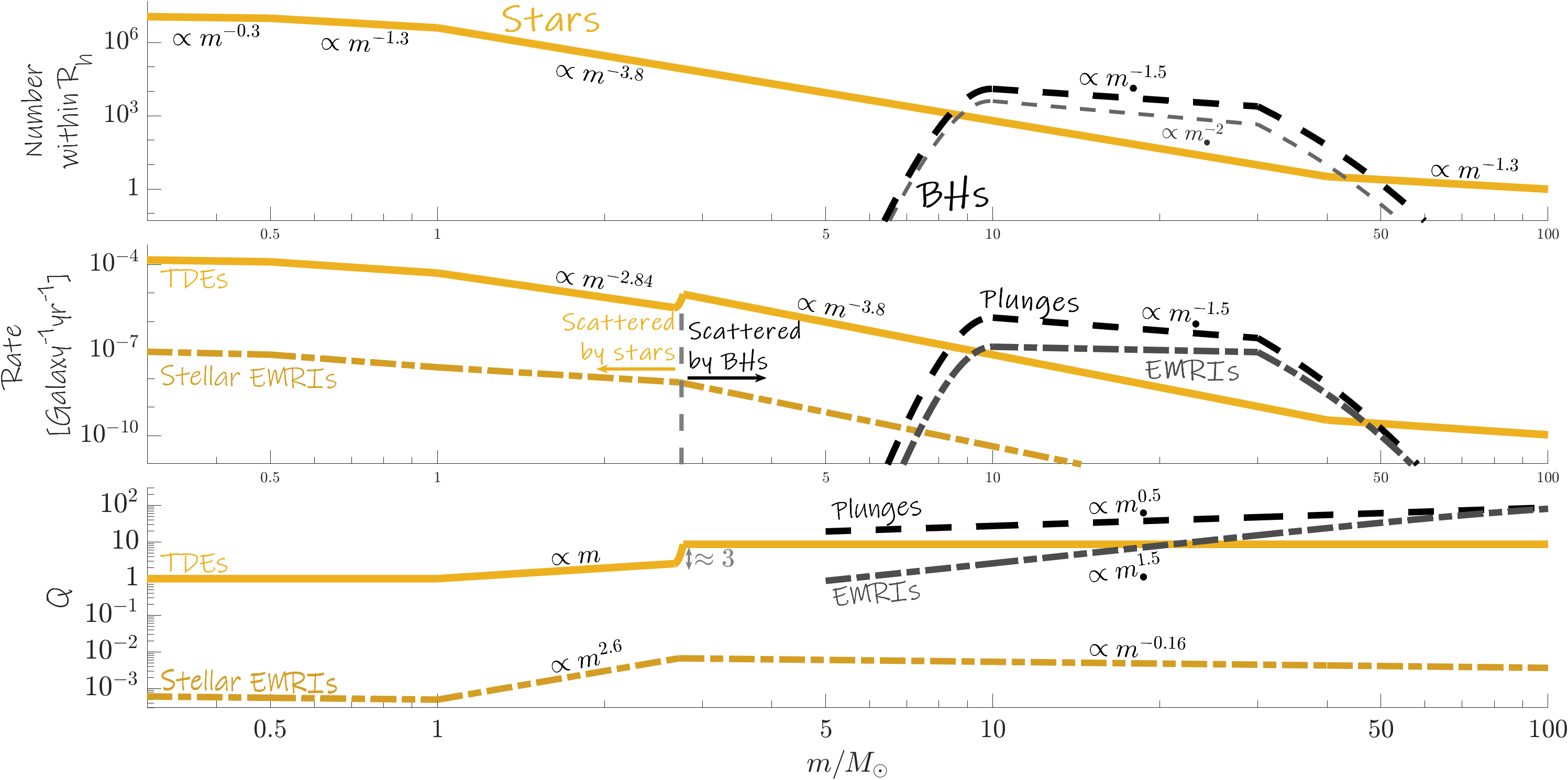
Figure 2: Distributions for stars (yellow lines) and BHs (dashed black lines). Top panel: The number, $N(m)=m{\rm d}N/{\rm d}m$, of stars and BHs within the sphere of influence. The stars follow the stellar PMF (Eq. 4). We show our assumed BH mass distribution (thin gray dashed line, Eq. 6), and its modification due to segregation from beyond the sphere of influence (thick black dashed line, Eq. 10). Second panel: The rates of TDEs, plunges, EMRIs, and sEMRIs. The dashed vertical gray line separates masses that are primarily scattered by stars ($m\lesssim 3$) from those mostly scattered by $30{M_{\odot}}$ BHs. Bottom panel: The enhancement factor $\mathcal{Q}$ for the different transients. Mass segregation within the sphere of influence generally leads to over-representation of transients involving massive stars, resulting in $\mathcal{Q}\approx 9$ for TDEs with $m\gtrsim 3$ (Eq. 18). sEMRIs are suppressed compared to TDEs, but also show over-representation of massive stars. However, for very massive stars ($m\gtrsim 3$), $\mathcal{Q}$ weakly decreases (Eq. 29), reflecting the variation of the tidal radius with stellar mass. For TDEs, $\mathcal{Q}$ sharply increases around $m\approx 3$, as indicated by the gray arrow, since these stars become mostly scattered by BHs. For BHs, segregation beyond the sphere of influence takes place as well, leading to an enhancement factor that increases with mass. For EMRIs, $\mathcal{Q}$ rises more steeply due to the additional dependence of the EMRI critical radius on the BH mass (Eq. 23).

We assume that the black hole mass distribution declines significantly outside the range $10\lesssim m_{\bullet}\lesssim 30$ and has little influence on our results. At the lower mass end, we adopt a minimal BH mass of $m_{\bullet}=5$ (consistent with the “lower mass gap”, see Abbott et al., 2023). This distribution is schematically presented in Fig. (2).

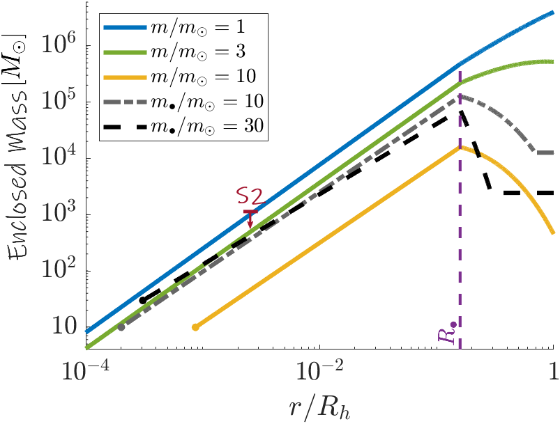
Figure 1: The enclosed mass of stars (solid colored lines) and BHs (dashed and dashed-dotted lines) as a function of semimajor axis $r$. The purple dashed vertical line marks $R_{\bullet}$ (Eq. 11), below which $30{M_{\odot}}$ BHs dominate the scattering and follow the BW profile. In this region, lighter stars and BHs follow shallower power-law profiles. At larger distances ($R_{\bullet}\lesssim r\lesssim R_{h}$), massive objects become exponentially rare as they segregate inward (as derived by Linial & Sari, 2022). The BH distribution flattens around $R_{h}$ due to the influx of BHs from greater distances. The red arrow indicates the observational upper limit for the extended mass enclosed within the orbit of S2 (Gravity Collaboration et al., 2024). The distributions are truncated once a single object remains.

2.3 Stellar Segregation

Assuming that the nuclear stellar cluster is dynamically relaxed, the stellar steady-state distribution satisfies a zero particle flux (Bahcall & Wolf, 1976, 1977; Linial & Sari, 2022), which corresponds to a constant, non-vanishing energy flux (Binney & Tremaine, 1987; Fragione & Sari, 2018; Rom et al., 2023).

Linial & Sari (2022) derived the zero-flux, steady-state solution for a power-law mass function and observed that weighting the segregated distribution by a factor of $m^{3/2}$ reproduces the single-mass BW profile. Here, we offer a simple explanation for this result, which allow us to apply it for the more realistic PMF, as given by Eq. (4).

We consider the constant energy flux through semimajor axis $r$. We assume that at each semimajor axis the energy flux is dominated by objects of mass $m$, where $m$ may be a function of $r$. For each mass group, the energy flux induced by self-scattering (i.e., scattering between objects of the same mass) is

$$\mathcal{F}_{E} \approx\frac{E(r,m)N_{\star}(m)}{\tau_{\rm rlx}(r,m)}$$ (7)

where $E(r,m)\propto m/r$ is the orbital energy, and $\tau_{\rm rlx}$ is the relaxation timescale. Furthermore, $\tau_{\rm rlx}$ is given by (Binney & Tremaine, 1987; Merritt et al., 2011; Sari & Fragione, 2019)

$$\tau_{\rm rlx}\left(r,m\right) \approx\frac{P(r)}{\log\Lambda}\frac{\left(M_{BH}/m\right)^{2}}{N\left(m\right)},$$ (8)

where $P(r)=\sqrt{r^{3}/\left(GM_{BH}\right)}$ is the orbital period, $N(m)=m{\rm d}N/{\rm d}m\propto m^{1-\gamma}$, and $\log\Lambda\sim\log\left(M_{BH}\right)$ is the Coulomb logarithm.

Combining Eqs. (7) and (8) we find the energy flux scales as $\mathcal{F}_{E}\propto m^{3}N^{2}r^{-5/2}$. Maintaining a constant energy flux, with a given mass spectrum (e.g., Eqs. 4 and 5), determines the density profile as well as the mass that dominates the scattering at each radius. In this interpretation, the effective cross-section of $m^{3/2}$, identified by Linial & Sari (2022), arises from the combination of the scattering cross-section, $\sigma\propto m^{2}$, and the orbital energy, $E\propto m$.

The constant energy flux solution naturally leads to mass-segregated distribution. Massive stars (with $m\gtrsim 1$) sink inward up to a characteristic distance $r_{d}(m)$ where their self-scattering dominate the energy flux. Using the mentioned scaling, together with the constant energy flux requirement and the stellar PMF, gives

$$\frac{r_{d}(m)}{R_{h}}\approx m^{2-4\gamma/5},$$ (9)

where one solar-mass stars, whose lifetime roughly equals the age of the galaxy, dominate at the radius of influence. This result reproduces the relation obtained by the detailed calculation of Linial & Sari (2022). As discussed below, the presence of a stellar-mass BH population alters this behavior for stars with masses $m\gtrsim 3$.

The spatial distribution of different stars and BHs is demonstrated in Fig. (1), where we present the enclosed mass as a function of the semimajor axis. Evidently, low-mass stars ($m\lesssim 1$) dominate the mass budget throughout most of the cluster. The contribution from more massive objects to the total enclosed mass becomes comparable to that of the low-mass stars around $r\sim 10^{-4}R_{h}$, where only a few of these massive objects reside.

Recent observations of the Milky Way’s center (Gravity Collaboration et al., 2024) impose an upper limit of about $1200{M_{\odot}}$ for the extended mass within the orbit of S2 (depicted by the red arrow in Fig. 1). Our segregated profile predicts an extended mass value similar to this upper limit, composed mostly of solar-mass stars. Notably, around S2’s semimajor axis, the density of $10{M_{\odot}}$ BHs is a factor of $\approx 30$ lower than that of the stars. Furthermore, without mass segregation, a BW profile of stars would predict a stellar density higher by a factor of $\approx 5$, in contrast with the observations.

2.4 BHs segregation

The assumption of a relaxed nuclear stellar cluster implies that massive objects can migrate into the sphere of influence during the galaxy lifetime. Beyond the radius of influence, the stellar distribution can be approximated as an isothermal sphere, where $N(r)\propto r$ and the relaxation timescale for objects of mass $m$ scales as $\tau_{\rm rlx}(r>R_{h},m)\propto r^{2}/m$ (Binney & Tremaine, 1987).

Therefore, more massive objects can segregate inwards from greater distances, scaling as $r\propto m^{1/2}$. This process increases the mass distribution of stellar mass black holes within the sphere of influence by a factor of $m_{\bullet}^{1/2}$, resulting in an effective power-law index

$$\widetilde{\gamma}_{\bullet}=\gamma_{\bullet}-\frac{1}{2}.$$ (10)

Thus, the BH number fraction inside the sphere of influence, $f^{\rm cusp}_{\bullet}$, is expected to be enhanced by $f^{\rm cusp}_{\bullet}/f^{\rm IMF}_{\bullet}\approx 3$ relative to its expected value from the (non-segregated) stellar IMF. This enhancement impacts the expected number of EMRIs that would be observed by LISA (Babak et al., 2017; Bonetti & Sesana, 2020; Pozzoli et al., 2023; Rom et al., 2024). Additionally, this incoming flux of BHs flattens their spatial distribution near the radius of influence, as schematically illustrated in Fig. (1).

Although massive stars may segregate from beyond the sphere of influence as well, we do not account for this effect in their distribution due to their short lifetimes and the uncertainty surrounding their migration mechanisms.

Within the sphere of influence, the BHs sink, due to dynamical friction from the stars, to a characteristic distance $R_{\bullet}$, where BHs with masses $\widetilde{m}_{\bullet}\approx 30$ become the dominant scatterers. This distance is determined by comparing the energy flux of BHs (analogous to Eq. 7) to the constant energy flux set by one solar-mass stars at the radius of influence. This yields

$$\frac{R_{\bullet}}{R_{h}}=\left(\frac{N_{\bullet}(\widetilde{m}_{\bullet})^{2}\widetilde{m}_{\bullet}^{3}}{M^{2}}\right)^{2/5}=\xi_{\bullet}^{4/5}=0.16.$$ (11)

As presented in Fig. (1), from $R_{\bullet}$ inward, the $30{M_{\odot}}$ BHs follow the single-mass BW profile, while lighter stars and BHs settle into shallower profiles (according to Eq. 1). Thus, massive stars with $m\gtrsim 3$ will accumulate around $R_{\bullet}$, where they will be scattered by the BHs, rather than efficiently segregating to $r_{d}(m)\lesssim R_{\bullet}$. The critical stellar mass is given by $\widetilde{m}=\xi_{\bullet}^{2/\left(5-2\gamma\right)}\approx 3$, satisfying $r_{d}(\widetilde{m})\approx R_{\bullet}$. Therefore, we conclude that in the segregated distribution, stars of mass $m$ are concentrated around a characteristic distance, $\widetilde{r}_{d}(m)$, given by

$$\widetilde{r}_{d}\approx\left\{\begin{tabular}[]{@{}c@{\quad}l@{}}$R_{h}$&$m\lesssim 1$\\ $r_{d}(m)$&$1\lesssim m\lesssim 3$\\ $R_{\bullet}$&$m\gtrsim 3$\\ \end{tabular}\right.,$$ (12)

where $r_{d}(m)$ and $R_{\bullet}$ are given in Eqs. (9) and (11), respectively.

Our results are weakly sensitive to the poorly known stellar-mass BH distribution as long as heavy $\approx 30{M_{\odot}}$ BHs are abundant enough to dominate the scattering, namely, $N_{\bullet}(30)/N_{\bullet}(10)\gtrsim 3^{-3/2}$. The observations of the LIGO-Virgo-KAGRA (LVK) collaboration (Abbott et al., 2023) suggest that this is indeed the case, if the binary merger population is a good representative of the overall mass distribution of stellar-mass BHs.

We consider a BH mass function with $\gamma_{\bullet}=3$, leading to $\widetilde{\gamma}_{\bullet}=5/2$, which represents the steepest power-law profile where $30{M_{\odot}}$ BHs dominate the scattering. We note that for steeper profiles, $\gamma_{\bullet}>3$, with the same BH number fraction, the $10{M_{\odot}}$ BHs become the dominant scatterers at $R_{\bullet}$, and the impact of more massive stellar-mass BHs diminishes, as they are rarer and more segregated. Namely, the more massive stellar-mass BHs may dominate the scattering only at smaller distances, $r<R_{\bullet}$, where fewer objects reside.

3 Transients mass-dependent rates

Based on the steady-state distributions of stars and BHs, the transients formation rates can be estimated using the two-body scattering induced flux (Wang & Merritt, 2004; Hopman & Alexander, 2005; Stone & Metzger, 2016). Here we generalize this concept by taking into account the mass segregation as a function of radius, and arrive at

$$\frac{{\rm d}\Gamma}{{\rm d}m}\approx\frac{{\rm d}N/{\rm d}m}{\tau_{\rm rlx}(r,m)\log\Lambda^{\prime}},$$ (13)

The logarithmic term in the denominator originates from the diffusive flux in angular momentum and is given by the log of the ratio between the orbital semi-major axis to the loss-cone size, $\left(R_{t}/r\right)$ for stars or $\left(4R_{s}/r\right)$ for BHs. This introduces a weak dependence on the energy (and, in the case of stars, on the stellar tidal radius), which we simplify by approximating the logarithmic term as a constant, equal to the Coulomb logarithm (i.e., $\log\Lambda^{\prime}\approx\log\Lambda$).

We estimate the rate of each transient type and object mass by evaluating Eq. (13) at the radius where it is maximal, as described below. Additionally, we define the enhancement factor $\mathcal{Q}$ as the ratio between the rate of a specific transient, involving stars or BHs, and their abundance in the total population

$$\mathcal{Q}=P(R_{h})M_{BH}\frac{{\rm d}\Gamma/{\rm d}m}{{\rm d}N/{\rm d}m}.$$ (14)

The normalization factor, $P(R_{h})M_{\rm MW}$, is roughly the number of one solar-mass stars at the radius of influence divided by their tidal disruption rate. It is set such that $\mathcal{Q}_{TDE}\left(1\right)=1$.

3.1 TDE rate

The majority of disrupted stars with masses in the range $1\lesssim m\lesssim 3$ originate from the vicinity of $r_{d}(m)$, as defined by Eq. (9), where they dominate the scatterings. In this region, the relaxation timescale (Eq. 8) is

$$\tau_{\rm rlx}\left(m\right)\sim 10m^{-\gamma/5}\left(\frac{M_{BH}}{M_{\rm MW}}\right)^{5/4}{\rm Gyr}.$$ (15)

At smaller distances, both their number and the two-body scattering flux decrease as a power-law, and at larger distances their number is exponentially suppressed (Linial & Sari, 2022).

Therefore, using Eqs. (4), (13), and (15), the mass-dependent tidal disruption rate is given by

$$\left.\frac{{\rm d}\Gamma}{{\rm d}m}\right|_{TDE} \approx\frac{{\rm d}N_{\star}/{\rm d}m}{\tau_{\rm rlx}\left(m\right)\log\Lambda}\approx\frac{m^{-4\gamma/5}}{P(R_{h})}$$ (16)

$$\approx 5\times 10^{-5}m^{-4\gamma/5}\left(\frac{M_{BH}}{M_{\rm MW}}\right)^{-1/4}{\rm yr^{-1}}.$$

Consequentially, the enhancement factor (defined in Eq. 14) is

$$\mathcal{Q}_{TDE}=m^{\gamma/5}.$$ (17)

Given that $\gamma\approx 5$ for this stellar mass range (Eq. 5), the TDE rate scales roughly as ${\rm d}\Gamma/{\rm d}m\propto m^{-4}$ and the enhancement factor is $\mathcal{Q}_{TDE}\simeq m$. Notably, the TDE rate, as well as the rates of EMRIs and plunges (calculated below), scales with the SMBH mass as $\Gamma\propto M_{BH}^{-1/4}$ (in agreement with previous results, e.g., Hopman & Alexander, 2005; Kochanek, 2016; Yao et al., 2023).

As discussed in §2.4, the presence of a BH population modifies the cusp within $R_{\bullet}$. The transition of massive stars ($m\gtrsim\widetilde{m}$) from being primarily self-scattered to being scattered by BHs results in a sharp increase in the enhancement factor around $R_{\bullet}$, $\delta\mathcal{Q}\approx\left(\widetilde{m}_{\bullet}/\widetilde{m}\right)^{1/2}\approx 3$. Therefore

$$\mathcal{Q}_{TDE}(m\gtrsim\widetilde{m}) =\mathcal{Q}_{TDE}(\widetilde{m})\delta\mathcal{Q}$$ (18)

$$=\widetilde{m}_{\bullet}^{1/2}\xi_{\bullet}^{1/\left(5-2\gamma\right)}\approx 9.$$

At the other end of the mass spectrum, the segregation of low-mass stars, with $m\lesssim 1$, is negligible. As a result, disrupted stars of such masses typically originate near the radius of influence, where they are scattered by the one solar-mass stars. Their disruption rate follows their mass function, $\left.{\rm d}\Gamma/{\rm d}m\right|_{TDE}\propto m^{-\gamma}$ and thus $\mathcal{Q}_{TDE}\left(m\lesssim 1\right)=1$.

The enhancement factor of stellar disruptions is illustrated in Fig. (2) and can be summarized as follows:

$$\mathcal{Q}_{TDE}\approx\left\{\begin{tabular}[]{@{}c@{\quad}l@{}}$1$&$m\lesssim 1$\\ $m$&$1\lesssim m\lesssim 3$\\ 9&$m\gtrsim 3$\\ \end{tabular}\right..$$ (19)

3.2 Plunge rate

The stellar-mass BHs are predominantly scattered by the $\widetilde{m}_{\bullet}\approx 30$ BHs near $R_{\bullet}$. Therefore, the relevant scattering timescale (Eq. 8) for the plunge rate is given by

$$\tau_{{\rm rlx},\bullet}\left(r\right) \approx\frac{P\big{(}r\big{)}}{\log\Lambda}\frac{\left(M_{BH}/\widetilde{m}_{\bullet}\right)^{2}}{N_{\bullet}\left(\widetilde{m}_{\bullet}\right)\left(r/R_{\bullet}\right)^{5/4}}$$ (20)

$$=\frac{P\big{(}R_{h}\big{)}M_{BH}}{\log\Lambda}\widetilde{m}_{\bullet}^{-1/2}\left(\frac{r}{R_{h}}\right)^{1/4}$$

$$\sim 1\ {\rm Gyr}\left(\frac{r}{R_{\bullet}}\right)^{1/4}\left(\frac{M_{BH}}{M_{\rm MW}}\right)^{5/4},$$

where we used Eqs. (8), (6) and (11).

The resulting plunge rate, for BHs in the mass range $10\lesssim m_{\bullet}\lesssim 30$, is

$$\left.\frac{{\rm d}\Gamma}{{\rm d}m}\right|_{Plunge} \approx\frac{{\rm d}N_{\bullet}/{\rm d}m_{\bullet}}{\log\Lambda\tau_{{\rm rlx},\bullet}(R_{\bullet})}\approx\frac{\xi_{\bullet}^{4/5}\widetilde{m}_{\bullet}^{1/2}m_{\bullet}^{-\widetilde{\gamma}_{\bullet}}}{P\left(R_{h}\right)}$$ (21)

$$\approx 10^{-7}\left(\frac{m_{\bullet}}{10}\right)^{-5/2}\left(\frac{M_{BH}}{M_{\rm MW}}\right)^{-1/4}{\rm yr^{-1}}.$$

Consequently, the enhancement factor is

$$\mathcal{Q}_{Plunge}\approx 27\left(\frac{m_{\bullet}}{10}\right)^{1/2}.$$ (22)

This scaling reflects the flattening of the BH mass spectrum caused by the segregation into the sphere of influence (see §2.4). It applies to both lighter and heavier BHs, as they are mostly scattered by BHs with mass $\widetilde{m}_{\bullet}$ around $R_{\bullet}$, leading to $\left.{\rm d}\Gamma/{\rm d}m\right|_{Plunge}\propto m_{\bullet}^{-\widetilde{\gamma}_{\bullet}}$.

3.3 EMRI rate

In order to estimate the EMRI rate, we first determine the characteristic radius, $R_{c}$, from which they originate (Hopman & Alexander, 2005; Amaro-Seoane, 2018; Sari & Fragione, 2019). This radius is defined such that the GW timescale and the scattering timescale are comparable for orbits with $r=R_{c}$ and $r_{p}=4R_{s}$ (for further details see Rom et al., 2024). It is given by

$$\frac{R_{c}}{R_{h}} \approx\left(\frac{m_{\bullet}}{16\sqrt{2}\log\Lambda\widetilde{m}_{\bullet}^{1/2}}\right)^{4/5}\approx 0.02\left(\frac{m_{\bullet}}{10}\right)^{4/5}.$$ (23)

This value is slightly lower than previous estimates (e.g., Hopman & Alexander, 2005; Rom et al., 2024; Kaur & Perets, 2024) due to the BH mass distribution we consider. Specifically, in our model, stellar-mass BHs are scattered by more massive $30{M_{\odot}}$ BHs, rather than the commonly assumed $10{M_{\odot}}$ BHs. The presence of more massive scatterers reduces the scattering timescale, leading to the smaller critical distance.

The EMRI rate for BHs in the mass range $10\lesssim m_{\bullet}\lesssim 30$ is therefore

$$\left.\frac{{\rm d}\Gamma}{{\rm d}m}\right|_{EMRI} \approx\frac{{\rm d}N_{\bullet}/{\rm d}m_{\bullet}\left(R_{c}/R_{\bullet}\right)^{3/2-m_{\bullet}/(4\widetilde{m}_{\bullet})}}{\log\Lambda\tau_{{\rm rlx},\bullet}\left(R_{c}\right)}$$ (24)

$$\approx 5\times 10^{-7}m_{\bullet}^{1-\widetilde{\gamma}_{\bullet}}\left(\frac{125}{m_{\bullet}}\right)^{m_{\bullet}/150}$$

$$\quad\times\left(\frac{M_{BH}}{M_{\rm MW}}\right)^{-1/4}{\rm yr^{-1}},$$

and the corresponding enhancement factor is

$$\mathcal{Q}_{EMRI} =0.07m_{\bullet}^{3/2}\left(\frac{125}{m_{\bullet}}\right)^{m_{\bullet}/150}\approx 2.7\left(\frac{m_{\bullet}}{10}\right)^{3/2}.$$ (25)

Thus, we get that for $10{M_{\odot}}$ BHs the EMRI rate is $\approx 10^{-8}\ {\rm yr^{-1}}$ and they are enhanced by a factor of $\mathcal{Q}_{EMRI}(10)\approx 2.7$. The scaling $\mathcal{Q}_{EMRI}\propto m_{\bullet}^{3/2}$ stems from two contributions: a factor of $m_{\bullet}^{1/2}$ due to the segregation beyond the sphere of influence (similar to the case of plunges), and a factor of $m_{\bullet}$ from the dependence of the critical radius on the BH mass (Eq. 23).

Furthermore, using Eqs. (21) and (24), we determine the EMRI-to-plunge ratio, a key parameter for predicting the number of sources detectable by LISA (see Babak et al., 2017; Rom et al., 2024)

$$\frac{\left.{\rm d}\Gamma/{\rm d}m\right|_{EMRI}}{\left.{\rm d}\Gamma/{\rm d}m\right|_{Plunge}} =\left(\frac{R_{c}}{R_{\bullet}}\right)^{\left(5-m_{\bullet}/\widetilde{m}_{\bullet}\right)/4}$$ (26)

$$\approx\left(\frac{m_{\bullet}}{125}\right)^{1-m_{\bullet}/150}.$$

For $10{M_{\odot}}$ BHs, Eq. (26) predicts an EMRI-to-plunge ratio of $\approx 0.1$. This estimate is consistent with the fiducial value considered by Babak et al. (2017) and is about $1.5$ times lower than the result of Rom et al. (2024), which was based on a two-mass model of the nuclear stellar cluster. The lower ratio arises because, in this work, the $10{M_{\odot}}$ BHs are scattered by heavier $30{M_{\odot}}$ BHs.

3.4 Stellar EMRI rate

Finally, we consider the case where a main sequence star slowly descends toward the SMBH due to GW emission, i.e., an EMRI of a main sequence star rather than of a BH. In this case, the critical semimajor axis is found by equating the minimal periapsis to the tidal radius (Linial & Sari, 2023), in contrast to $4R_{s}$ as in the BH case. This yields

$$\frac{R_{\star,c}}{R_{h}} \approx\left(190\widetilde{m}_{\bullet}^{1/2}\log\Lambda\right)^{-4/5}m^{-0.13}\left(\frac{M_{BH}}{M_{\rm MW}}\right)^{4/3}$$ (27)

$$\approx 6\times 10^{-4}m^{-0.13}\left(\frac{M_{BH}}{M_{\rm MW}}\right)^{4/3}.$$

The resulting main sequence stellar EMRI (sEMRI) rate is

$$\left.\frac{{\rm d}\Gamma}{{\rm d}m}\right|_{sEMRI} \approx\frac{{\rm d}N_{\star}/{\rm d}m\left(R_{\star,c}/\widetilde{r}_{d}\right)^{3/2}}{\log\Lambda\tau_{{\rm rlx},\bullet}\left(R_{\star,c}\right)}$$ (28)

$$\approx 2.5\times 10^{-8}m^{-\gamma-0.16}\left(\frac{M_{BH}}{M_{\rm MW}}\right)^{17/12}{\rm yr^{-1}}$$

$$\ \ \times\left\{\begin{tabular}[]{@{}c@{\quad}l@{}}$1$&$m\lesssim 1$\\ $m^{6\gamma/5-3}$&$1\lesssim m\lesssim 3$\\ $16$&$m\gtrsim 3$\\ \end{tabular}\right.,$$

where we assume that stars of mass $m$ are concentrated around $\widetilde{r}_{d}(m)$, as given in Eq. (12). The calculation is further simplified by assuming that for $r\lesssim\widetilde{r}_{d}$ the stellar number density scales as $r^{-3/2}$, neglecting the mass-dependent correction to the power of the density profile (Eq. 1).

The weak $m^{-0.16}$ scaling of the sEMRI rate arises from the critical radius $R_{\star,c}$ (Eq. 27). This reflects the tidal radii variation across different stellar masses, and, hence, implicitly depends on the stellar mass-radius relation. The additional mass-dependent term in the intermediate mass range, $1\lesssim m\lesssim 3$, arises from the segregated location of these stars.

The sEMRI rate in our model is smaller compared to calculations assuming a single-mass nuclear stellar cluster (Linial & Sari, 2023) or a two-mass model (Kaur et al., 2024). This is because, in our model, the stars are scattered by more massive BHs, which shortens the scattering timescale and reduce the critical distance for EMRI formation, shifting it to regions where stars are less abundant.

From Eqs. (14) and (28), the sEMRI enhancement factor is

$$\mathcal{Q}_{sEMRI}\approx 5\times 10^{-4}m^{-0.16}\times\left\{\begin{tabular}[]{@{}c@{\quad}l@{}}$1$&$m\lesssim 1$\\ $m^{2.8}$&$1\lesssim m\lesssim 3$\\ $16$&$m\gtrsim 3$\\ \end{tabular}\right..$$ (29)

Besides being mHz GW sources, relevant for space-based GW observatories, sEMRIs have recently gained attention as a potential origin of the observed QPEs (Zhao et al., 2021; Linial & Sari, 2023; Lu & Quataert, 2023; Linial & Metzger, 2023; Nicholl et al., 2024). Specifically, Linial & Metzger (2023) associated QPEs with the interaction between a stellar EMRI and a TDE accretion disk.

Given this interpretation, the QPE rate can be estimated by combining the TDE rate (Eq. 21), the sEMRI rate (Eq. 28), and the characteristic EMRI lifetime, $\tau_{GW}\sim m^{-1}{\rm Myr}$ (Linial & Metzger, 2023; Kaur et al., 2024). This yields a characteristic rate $\sim 10^{-6}\rm yr^{-1}$ for one solar-mass stars, roughly compatible with the observational inferred rate (Arcodia et al., 2024b).

The QPE rate scales as $m^{-1}\left.{\rm d}\Gamma/{\rm d}m\right|_{sEMRI}$, suggesting that low-mass stars (with $m\lesssim 1$) may be preferable candidates, based only on rate considerations.

We note that beyond the dynamical processes considered in this work, the effects of stellar binaries and collisions should be incorporated for a more detailed analysis of the sEMRIs formation mechanism. For example, binary tidal break-up may be a more efficient formation channel (Linial & Sari, 2023; Lu & Quataert, 2023), while collisions are expected to reduce the abundance of stars on tightly bound orbits, suppressing the sEMRI rate (Sari & Fragione, 2019; Rose et al., 2023; Balberg & Yassur, 2023; Balberg, 2023).

4 Discussion & Summary

We study the distributions of stars and BHs in nuclear stellar clusters surrounding SMBHs. We highlight the impact of mass segregation on the rates of TDEs, plunges, and EMRIs.

We assume that the cluster is dynamically relaxed, with stars following a PMF that accounts for their finite lifetimes, resulting in a steeper slope for $m\gtrsim 1$ relative to the stellar IMF. This working assumption is motivated by observations of massive stars in the central parsec of our galaxy (Ghez et al., 2003; Lu et al., 2006; Genzel et al., 2010). However, it should be revisited once the presence of massive stars deep in the sphere of influence, the so-called “paradox of youth”, is better understood.

Furthermore, we assume that $30{M_{\odot}}$ BHs are sufficiently abundant to dominate over all other stellar-mass BHs. This is inspired by the emerging BH mass spectrum, inferred from the observations of the LVK collaboration (Abbott et al., 2023). Given this assumption, the specific details of the BH distribution – taken here as a power-law toy model with tails extending to both low and high mass ends – affect the quantitative rate estimates but do not alter the qualitative trends discussed in this work.

We present a simple derivation of the segregated steady-state stellar distribution, in agreement with a previous analytic calculation of Linial & Sari (2022). Additionally, we schematically outline the BH distribution and its impact on the stellar distribution, consistently accounting for the mutual interactions between BHs and stars.

Accounting for the stellar-mass BHs, we show that their number within the sphere of influence increases by a factor of $\approx 3$ relative to the expected number based on the stellar IMF, as their relaxation time is shorter than the age of the galaxy, even outside the sphere of influence, allowing them to sink inwards from greater distances.

We further estimate the EMRI-to-plunge ratio and show that scattering by more massive BHs reduces the EMRI rate. This is because the scattering by heavier BHs shifts the EMRIs critical radius toward smaller distances, where the BH population is less abundant. Nonetheless, the segregated BH distribution leads to an over-representation of EMRIs and plunges involving massive stellar-mass BHs, with enhancement factor scaling as $\mathcal{Q}_{EMRI}\propto m_{\bullet}^{3/2}$ and $\mathcal{Q}_{Plunge}\propto m_{\bullet}^{1/2}$, respectively. These results are of particular interest, as they influence the expected number of EMRIs to be measured by LISA (Babak et al., 2017; Amaro-Seoane et al., 2023; Rom et al., 2024).

Regarding TDEs, we show that massive stars, with masses $1\lesssim m\lesssim 3$, have an enhanced disruption rate, compared to their abundance in the stellar population, by roughly a factor of $\mathcal{Q}_{TDE}=m$. This enhancement arises from segregation within the sphere of influence, leading to an accumulation of massive stars at smaller distances, where the scattering timescale is shorter. The disruption of more massive stars, with $m\gtrsim 3$, is enhanced by a constant factor of $\approx 9$, as they are predominantly scattered by BHs around a characteristic distance of $R_{\bullet}\sim 0.1R_{h}$.

Observationally, the tidal disruption rate of massive stars is not well constrained. Mass estimates of disrupted stars, based on the lightcurves of approximately 20 observed TDEs, generally indicate a preference for lower-mass stars, with a probability tail extending to more massive ones (Mockler et al., 2019; Ryu et al., 2020; Zhou et al., 2021). Additionally, Hinkle et al. (2024) and Wiseman et al. (2024) detected several long-lived luminous flares, which they suggest may originate from the disruption of stars with masses of $m\approx 3-10$. Mockler et al. (2022) identified a preference for the disruption of moderately massive stars, with $m\gtrsim 2$, relative to their prevalence in the stellar population, based on the nitrogen-to-carbon abundances in a few observed TDEs. Our analysis shows that this trend is expected due to mass segregation, which enhances the rate of such events.

Finally, we estimate the sEMRI rate, showing that it favors low-mass stars ($m\lesssim 1$). We find that the sEMRI rate is reduced compared to its expected rate from single-mass models (e.g., Linial & Sari, 2023), yet remains marginally consistent with the observationally inferred QPE rate (Arcodia et al., 2024b). However, a more detailed analysis, including the effects of stellar binaries and collisions (Rose et al., 2023; Balberg & Yassur, 2023; Balberg, 2023), is necessary for accurately determining the sEMRI rate.

Future observations, combined with a more detailed model of stellar and BH distributions, will clarify the extent of relaxation and mass segregation in galactic centers. These efforts will also determine whether the observed disruptions of massive stars can be fully attributed to mass segregation, or if additional factors, such as a recent star formation burst, are required.

References

- Abbott et al. (2023) Abbott, R., Abbott, T. D., Acernese, F., et al. 2023, Physical Review X, 13, 011048, doi: 10.1103/PhysRevX.13.011048
- Aharon & Perets (2016) Aharon, D., & Perets, H. B. 2016, ApJ, 830, L1, doi: 10.3847/2041-8205/830/1/L1
- Alexander (2017) Alexander, T. 2017, ARA&A, 55, 17, doi: 10.1146/annurev-astro-091916-055306
- Alexander & Hopman (2009) Alexander, T., & Hopman, C. 2009, ApJ, 697, 1861, doi: 10.1088/0004-637X/697/2/1861
- Amaro-Seoane (2018) Amaro-Seoane, P. 2018, Living Reviews in Relativity, 21, 4, doi: 10.1007/s41114-018-0013-8
- Amaro-Seoane & Preto (2011) Amaro-Seoane, P., & Preto, M. 2011, Classical and Quantum Gravity, 28, 094017, doi: 10.1088/0264-9381/28/9/094017
- Amaro-Seoane et al. (2017) Amaro-Seoane, P., Audley, H., Babak, S., et al. 2017, arXiv e-prints, arXiv:1702.00786, doi: 10.48550/arXiv.1702.00786
- Amaro-Seoane et al. (2023) Amaro-Seoane, P., Andrews, J., Arca Sedda, M., et al. 2023, Living Reviews in Relativity, 26, 2, doi: 10.1007/s41114-022-00041-y
- Arca Sedda et al. (2023) Arca Sedda, M., Naoz, S., & Kocsis, B. 2023, Universe, 9, 138, doi: 10.3390/universe9030138
- Arcodia et al. (2021) Arcodia, R., et al. 2021, Nature, 592, 704, doi: 10.1038/s41586-021-03394-6
- Arcodia et al. (2022) Arcodia, R., Miniutti, G., Ponti, G., et al. 2022, A&A, 662, A49, doi: 10.1051/0004-6361/202243259
- Arcodia et al. (2024a) Arcodia, R., Liu, Z., Merloni, A., et al. 2024a, arXiv e-prints, arXiv:2401.17275, doi: 10.48550/arXiv.2401.17275
- Arcodia et al. (2024b) Arcodia, R., Merloni, A., Buchner, J., et al. 2024b, A&A, 684, L14, doi: 10.1051/0004-6361/202348949
- Babak et al. (2017) Babak, S., Gair, J., Sesana, A., et al. 2017, Phys. Rev. D, 95, 103012, doi: 10.1103/PhysRevD.95.103012
- Bahcall & Wolf (1976) Bahcall, J. N., & Wolf, R. A. 1976, ApJ, 209, 214, doi: 10.1086/154711
- Bahcall & Wolf (1977) —. 1977, ApJ, 216, 883, doi: 10.1086/155534
- Balberg (2023) Balberg, S. 2023, arXiv e-prints, arXiv:2311.00497, doi: 10.48550/arXiv.2311.00497
- Balberg & Yassur (2023) Balberg, S., & Yassur, G. 2023, The Astrophysical Journal, 952, 149, doi: 10.3847/1538-4357/acdd73
- Bellm et al. (2019) Bellm, E. C., Kulkarni, S. R., Barlow, T., et al. 2019, Publications of the Astronomical Society of the Pacific, 131, 068003, doi: 10.1088/1538-3873/ab0c2a
- Binney & Tremaine (1987) Binney, J., & Tremaine, S. 1987, Galactic dynamics
- Bonetti & Sesana (2020) Bonetti, M., & Sesana, A. 2020, Phys. Rev. D, 102, 103023, doi: 10.1103/PhysRevD.102.103023
- Bortolas et al. (2023) Bortolas, E., Ryu, T., Broggi, L., & Sesana, A. 2023, Monthly Notices of the Royal Astronomical Society, 524, 3026, doi: 10.1093/mnras/stad2024
- Bricman & Gomboc (2020) Bricman, K., & Gomboc, A. 2020, The Astrophysical Journal, 890, 73, doi: 10.3847/1538-4357/ab6989
- Broggi et al. (2022) Broggi, L., Bortolas, E., Bonetti, M., Sesana, A., & Dotti, M. 2022, MNRAS, 514, 3270, doi: 10.1093/mnras/stac1453
- Bykov et al. (2024) Bykov, S., Gilfanov, M., Sunyaev, R., & Medvedev, P. 2024, arXiv e-prints, arXiv:2409.16908, doi: 10.48550/arXiv.2409.16908
- Chakraborty et al. (2021) Chakraborty, J., Kara, E., Masterson, M., et al. 2021, ApJ, 921, L40, doi: 10.3847/2041-8213/ac313b
- Chakraborty et al. (2024) Chakraborty, J., Arcodia, R., Kara, E., et al. 2024, ApJ, 965, 12, doi: 10.3847/1538-4357/ad2941
- Fragione & Sari (2018) Fragione, G., & Sari, R. 2018, The Astrophysical Journal, 852, 51, doi: 10.3847/1538-4357/aaa0d7
- Franchini et al. (2023) Franchini, A., Bonetti, M., Lupi, A., et al. 2023, A&A, 675, A100, doi: 10.1051/0004-6361/202346565
- Fujii et al. (2010) Fujii, M., Iwasawa, M., Funato, Y., & Makino, J. 2010, The Astrophysical Journal, 716, L80–L84, doi: 10.1088/2041-8205/716/1/l80
- Generozov & Madigan (2020) Generozov, A., & Madigan, A.-M. 2020, ApJ, 896, 137, doi: 10.3847/1538-4357/ab94bc
- Genzel et al. (2010) Genzel, R., Eisenhauer, F., & Gillessen, S. 2010, Reviews of Modern Physics, 82, 3121, doi: 10.1103/RevModPhys.82.3121
- Gezari (2021) Gezari, S. 2021, Annual Review of Astronomy and Astrophysics, 59, 21, doi: 10.1146/annurev-astro-111720-030029
- Ghez et al. (2003) Ghez, A. M., Duchêne, G., Matthews, K., et al. 2003, ApJ, 586, L127, doi: 10.1086/374804
- Ghez et al. (2008) Ghez, A. M., Salim, S., Weinberg, N. N., et al. 2008, ApJ, 689, 1044, doi: 10.1086/592738
- Gillessen et al. (2009) Gillessen, S., Eisenhauer, F., Trippe, S., et al. 2009, ApJ, 692, 1075, doi: 10.1088/0004-637X/692/2/1075
- Ginsburg & Loeb (2006) Ginsburg, I., & Loeb, A. 2006, Monthly Notices of the Royal Astronomical Society, 368, 221, doi: 10.1111/j.1365-2966.2006.10091.x
- Gould & Quillen (2003) Gould, A., & Quillen, A. C. 2003, The Astrophysical Journal, 592, 935, doi: 10.1086/375840
- Gravity Collaboration et al. (2024) Gravity Collaboration, Abd El Dayem, K., Abuter, R., et al. 2024, A&A, 692, A242, doi: 10.1051/0004-6361/202452274
- Hammerstein et al. (2023) Hammerstein, E., van Velzen, S., Gezari, S., et al. 2023, ApJ, 942, 9, doi: 10.3847/1538-4357/aca283
- Hills (1975) Hills, J. G. 1975, Nature, 254, 295, doi: 10.1038/254295a0
- Hinkle et al. (2024) Hinkle, J. T., Shappee, B. J., Auchettl, K., et al. 2024, arXiv e-prints, arXiv:2405.08855, doi: 10.48550/arXiv.2405.08855
- Holoien et al. (2015) Holoien, T. W.-S., Kochanek, C. S., Prieto, J. L., et al. 2015, Monthly Notices of the Royal Astronomical Society, 455, 2918, doi: 10.1093/mnras/stv2486
- Hopman & Alexander (2005) Hopman, C., & Alexander, T. 2005, The Astrophysical Journal, 629, 362, doi: 10.1086/431475
- Hopman & Alexander (2006) —. 2006, The Astrophysical Journal, 645, L133, doi: 10.1086/506273
- Ivezic et al. (2019) Ivezic, Z., Kahn, S. M., Tyson, J. A., et al. 2019, The Astrophysical Journal, 873, 111, doi: 10.3847/1538-4357/ab042c
- Jayasinghe et al. (2018) Jayasinghe, T., Kochanek, C. S., Stanek, K. Z., et al. 2018, MNRAS, 477, 3145, doi: 10.1093/mnras/sty838
- Kaur & Perets (2024) Kaur, K., & Perets, H. B. 2024, ApJ, 977, 8, doi: 10.3847/1538-4357/ad89bd
- Kaur et al. (2024) Kaur, K., Rom, B., & Sari, R. 2024, arXiv e-prints, arXiv:2406.07627. https://arxiv.org/abs/2406.07627
- Kaur et al. (2023) Kaur, K., Stone, N. C., & Gilbaum, S. 2023, MNRAS, 524, 1269, doi: 10.1093/mnras/stad1894
- Keshet et al. (2009) Keshet, U., Hopman, C., & Alexander, T. 2009, ApJ, 698, L64, doi: 10.1088/0004-637X/698/1/L64
- King (2022) King, A. 2022, MNRAS, 515, 4344, doi: 10.1093/mnras/stac1641
- Kochanek (2016) Kochanek, C. S. 2016, Monthly Notices of the Royal Astronomical Society, 461, 371, doi: 10.1093/mnras/stw1290
- Kormendy & Ho (2013) Kormendy, J., & Ho, L. C. 2013, Annual Review of Astronomy and Astrophysics, 51, 511, doi: 10.1146/annurev-astro-082708-101811
- Kroupa (2001) Kroupa, P. 2001, Monthly Notices of the Royal Astronomical Society, 322, 231, doi: 10.1046/j.1365-8711.2001.04022.x
- Levin (2006) Levin, Y. 2006, Monthly Notices of the Royal Astronomical Society, 374, 515, doi: 10.1111/j.1365-2966.2006.11155.x
- Levin & Beloborodov (2003) Levin, Y., & Beloborodov, A. M. 2003, The Astrophysical Journal, 590, L33–L36, doi: 10.1086/376675
- Lightman & Shapiro (1977) Lightman, A. P., & Shapiro, S. L. 1977, ApJ, 211, 244, doi: 10.1086/154925
- Linial & Metzger (2023) Linial, I., & Metzger, B. D. 2023, ApJ, 957, 34, doi: 10.3847/1538-4357/acf65b
- Linial & Sari (2022) Linial, I., & Sari, R. 2022, ApJ, 940, 101, doi: 10.3847/1538-4357/ac9bfd
- Linial & Sari (2023) —. 2023, ApJ, 945, 86, doi: 10.3847/1538-4357/acbd3d
- Lu et al. (2006) Lu, J. R., Ghez, A. M., Hornstein, S. D., et al. 2006, in Journal of Physics Conference Series, Vol. 54, Journal of Physics Conference Series, ed. R. Schödel, G. C. Bower, M. P. Muno, S. Nayakshin, & T. Ott (IOP), 279–287, doi: 10.1088/1742-6596/54/1/044
- Lu & Quataert (2023) Lu, W., & Quataert, E. 2023, MNRAS, 524, 6247, doi: 10.1093/mnras/stad2203
- Luo et al. (2016) Luo, J., Chen, L.-S., Duan, H.-Z., et al. 2016, Classical and Quantum Gravity, 33, 035010, doi: 10.1088/0264-9381/33/3/035010
- Magorrian & Tremaine (1999) Magorrian, J., & Tremaine, S. 1999, MNRAS, 309, 447, doi: 10.1046/j.1365-8711.1999.02853.x
- Mancieri et al. (2024) Mancieri, D., Broggi, L., Bonetti, M., & Sesana, A. 2024, arXiv e-prints, arXiv:2409.09122, doi: 10.48550/arXiv.2409.09122
- Mapelli (2021) Mapelli, M. 2021, in Handbook of Gravitational Wave Astronomy, 16, doi: 10.1007/978-981-15-4702-7_16-1
- Merritt (2004) Merritt, D. 2004, in Coevolution of Black Holes and Galaxies, ed. L. C. Ho, 263, doi: 10.48550/arXiv.astro-ph/0301257
- Merritt et al. (2011) Merritt, D., Alexander, T., Mikkola, S., & Will, C. M. 2011, Phys. Rev. D, 84, 044024, doi: 10.1103/PhysRevD.84.044024
- Metzger et al. (2022) Metzger, B. D., Stone, N. C., & Gilbaum, S. 2022, ApJ, 926, 101, doi: 10.3847/1538-4357/ac3ee1
- Miller & Scalo (1979) Miller, G. E., & Scalo, J. M. 1979, ApJS, 41, 513, doi: 10.1086/190629
- Milosavljević & Loeb (2004) Milosavljević, M., & Loeb, A. 2004, The Astrophysical Journal, 604, L45, doi: 10.1086/383467
- Miniutti et al. (2023) Miniutti, G., Giustini, M., Arcodia, R., et al. 2023, A&A, 670, A93, doi: 10.1051/0004-6361/202244512
- Miniutti et al. (2019) Miniutti, G., Saxton, R. D., Giustini, M., et al. 2019, Nature, 573, 381, doi: 10.1038/s41586-019-1556-x
- Miniutti, G. et al. (2023) Miniutti, G., Giustini, M., Arcodia, R., et al. 2023, A&A, 674, L1, doi: 10.1051/0004-6361/202346653
- Mockler et al. (2019) Mockler, B., Guillochon, J., & Ramirez-Ruiz, E. 2019, ApJ, 872, 151, doi: 10.3847/1538-4357/ab010f
- Mockler et al. (2022) Mockler, B., Twum, A. A., Auchettl, K., et al. 2022, ApJ, 924, 70, doi: 10.3847/1538-4357/ac35d5
- Nicholl et al. (2024) Nicholl, M., Pasham, D. R., Mummery, A., et al. 2024, Nature, 634, 804, doi: 10.1038/s41586-024-08023-6
- Pan et al. (2022) Pan, X., Li, S.-L., Cao, X., Miniutti, G., & Gu, M. 2022, ApJ, 928, L18, doi: 10.3847/2041-8213/ac5faf
- Peebles (1972) Peebles, P. J. E. 1972, ApJ, 178, 371, doi: 10.1086/151797
- Perets et al. (2007) Perets, H. B., Hopman, C., & Alexander, T. 2007, The Astrophysical Journal, 656, 709, doi: 10.1086/510377
- Pozzoli et al. (2023) Pozzoli, F., Babak, S., Sesana, A., Bonetti, M., & Karnesis, N. 2023, Phys. Rev. D, 108, 103039, doi: 10.1103/PhysRevD.108.103039
- Quintin et al. (2023) Quintin, E., Webb, N. A., Guillot, S., et al. 2023, A&A, 675, A152, doi: 10.1051/0004-6361/202346440
- Qunbar & Stone (2023) Qunbar, I., & Stone, N. C. 2023, arXiv e-prints, arXiv:2304.13062, doi: 10.48550/arXiv.2304.13062
- Raj & Nixon (2021) Raj, A., & Nixon, C. J. 2021, The Astrophysical Journal, 909, 82, doi: 10.3847/1538-4357/abdc25
- Raveh & Perets (2021) Raveh, Y., & Perets, H. B. 2021, MNRAS, 501, 5012, doi: 10.1093/mnras/staa4001
- Rees (1988) Rees, M. J. 1988, Nature, 333, 523, doi: 10.1038/333523a0
- Rom et al. (2024) Rom, B., Linial, I., Kaur, K., & Sari, R. 2024, ApJ, 977, 7, doi: 10.3847/1538-4357/ad8b1d
- Rom et al. (2023) Rom, B., Linial, I., & Sari, R. 2023, The Astrophysical Journal, 951, 14, doi: 10.3847/1538-4357/acd54f
- Rose et al. (2023) Rose, S. C., Naoz, S., Sari, R., & Linial, I. 2023, The Astrophysical Journal, 955, 30, doi: 10.3847/1538-4357/acee75
- Ryu et al. (2020) Ryu, T., Krolik, J., & Piran, T. 2020, The Astrophysical Journal, 904, 73, doi: 10.3847/1538-4357/abbf4d
- Sanyal et al. (2015) Sanyal, D., Grassitelli, L., Langer, N., & Bestenlehner, J. M. 2015, A&A, 580, A20, doi: 10.1051/0004-6361/201525945
- Sari & Fragione (2019) Sari, R., & Fragione, G. 2019, ApJ, 885, 24, doi: 10.3847/1538-4357/ab43df
- Stone & Metzger (2016) Stone, N. C., & Metzger, B. D. 2016, MNRAS, 455, 859, doi: 10.1093/mnras/stv2281
- Stone et al. (2020) Stone, N. C., Vasiliev, E., Kesden, M., et al. 2020, Space Sci. Rev., 216, 35, doi: 10.1007/s11214-020-00651-4
- van Velzen (2018) van Velzen, S. 2018, ApJ, 852, 72, doi: 10.3847/1538-4357/aa998e
- van Velzen et al. (2011) van Velzen, S., Farrar, G. R., Gezari, S., et al. 2011, The Astrophysical Journal, 741, 73, doi: 10.1088/0004-637X/741/2/73
- Vasiliev & Merritt (2013) Vasiliev, E., & Merritt, D. 2013, ApJ, 774, 87, doi: 10.1088/0004-637X/774/1/87
- Wang & Merritt (2004) Wang, J., & Merritt, D. 2004, ApJ, 600, 149, doi: 10.1086/379767
- Wiseman et al. (2024) Wiseman, P., Williams, R. D., Arcavi, I., et al. 2024, arXiv e-prints, arXiv:2406.11552, doi: 10.48550/arXiv.2406.11552
- Xian et al. (2021) Xian, J., Zhang, F., Dou, L., He, J., & Shu, X. 2021, ApJ, 921, L32, doi: 10.3847/2041-8213/ac31aa
- Yao et al. (2023) Yao, Y., Ravi, V., Gezari, S., et al. 2023, The Astrophysical Journal Letters, 955, L6, doi: 10.3847/2041-8213/acf216
- Zhao et al. (2021) Zhao, Z. Y., Wang, Y. Y., Zou, Y. C., Wang, F. Y., & Dai, Z. G. 2021, arXiv e-prints, arXiv:2109.03471. https://arxiv.org/abs/2109.03471
- Zhou et al. (2021) Zhou, Z. Q., Liu, F. K., Komossa, S., et al. 2021, ApJ, 907, 77, doi: 10.3847/1538-4357/abcccb