Wormholes in finite cutoff JT gravity: A study of baby universes and (Krylov) complexity

Abstract

In this paper, as an application of the ‘Complexity = Volume’ proposal, we calculate the growth of the interior of a black hole at late times for finite cutoff JT gravity. Due to this integrable, irrelevant deformation, the spectral properties are modified non-trivially. The Einstein-Rosen Bridge (ERB) length saturates faster than pure JT gravity. We comment on the possible connection between Krylov Complexity and ERB length for deformed theory. Apart from this, we calculate the emission probability of baby universes for the deformed theory and make remarks on its implications for the ramp of the Spectral Form Factor. Finally, we compute the correction to the volume of the moduli space due to the non-perturbative change of the spectral curve because of the finite cutoff at the boundary.

1 Introduction

Although a microscopic understanding of the universe has eluded fundamental physics for decades, accelerated progress has been made in recent times in the context of the AdS/CFT correspondence Maldacena:1997re ; Witten:1998qj . There is a renewed interest in lower-dimensional models of quantum gravity in two dimensions Jackiw:1984je ; Teitelboim:1983ux ; Almheiri:2014cka as well as in three dimensions, pioneered in Maloney:2007ud ; Yin:2007gv and more recently Collier:2023fwi ; deBoer:2024mqg ; Collier:2024mgv ; Bhattacharyya:2024vnw ; Post:2024itb ; Takahashi:2024ukk . Particularly in two-dimensions, Jackiw-Teitelboim (JT) gravity Jackiw:1984je ; Teitelboim:1983ux , a model of dilaton gravity in a 2D Euclidean spacetime of negative cosmological constant. Its connection to the Sachdev-Ye-Kitaev (SYK) model Sachdev:1992fk ; 2015escq.progE…2K ; 2015escq.progE..38K ; Sachdev:2015efa has helped characterize its chaotic nature and has become a topic of active research interest Shenker:2014cwa ; Maldacena:2015waa ; Stanford:2015owe ; Cotler:2016fpe ; Jensen:2016pah ; Engelsoy:2016xyb ; Chowdhury:2017jzb ; Altland:2022xqx . This connection is enabled by the fact that the low-energy dynamics of the SYK model are described by the 1D Schwarzian theory, which in turn is the boundary description of bulk 2D JT gravity 2015escq.progE…2K ; 2015escq.progE..38K ; Maldacena:2016hyu ; Maldacena:2016upp ; Kourkoulou:2017zaj ; Kitaev:2017awl ; Mertens:2018fds ; Lin:2019qwu . This has also led to the study of gravity in the context of random matrix theories Cotler:2016fpe ; Saad:2018bqo . The seminal work of Saad-Shenker-Stanford Saad:2019lba , has further established the connection between JT gravity, matrix integrals and topological recursion Stanford:2019vob ; Eynard:2007fi .

The study of perturbations of black holes has taken a central role in key problems such as the black hole information paradox Hawking:1976ra ; Mathur:2009hf ; Raju:2020smc since the introduction of the AdS/CFT duality Maldacena:2001kr . Two-point functions of quantum fields outside the eternal black hole, widely separated in time, are used to study perturbations in the black hole. While semi-classical analysis suggests a two-point function that decays forever, such functions for the boundary theory on a compact space with a discrete spectrum point to saturation at late times Maldacena:2001kr ; Goheer:2002vf ; Dyson:2002pf ; Barbon:2003aq . The precise analytic description of the two-point function is challenging to obtain since the fluctuations around the late-time average are highly erratic and sensitive to the fine details of the energy spectrum Barbon:2003aq ; prange1997spectral . This behaviour can be studied more readily by recasting it as a problem in random matrix theory and the SYK model. Such studies indicate that the two-point function decays initially, then shows a period of linear growth, called the ‘ramp’ until the growth finally stops at a time exponentially long in the entropy, which is referred to as the ‘plateau’ Cotler:2016fpe .

This non-decaying behaviour of correlation functions in JT gravity Maldacena:2016upp ; Yang:2018gdb ; Gross:2017aos ; Lam:2018pvp ; Mertens:2017mtv ; Blommaert:2018oro ; Blommaert:2019hjr ; Bulycheva:2019naf ; Iliesiu:2019xuh is attributed to the topology change due to Euclidean wormholes on the bulk Lavrelashvili:1987jg ; HAWKING1987337 ; GIDDINGS1988890 ; Coleman:1988cy ; COLEMAN1988643 ; GIDDINGS1989481 ; KLEBANOV1989665 ; Maldacena:2004rf ; Arkani-Hamed:2007cpn . This is regarded as a tunneling process in which an asymptotically AdS ‘parent universe’ emits or absorbs a closed ‘baby universe’. Such baby universes can also form ‘loops’ when they are reabsorbed after getting emitted, or they can end in a ‘D-brane’ state. The behaviour of the spectral form factor can also be attributed to this process Saad:2018bqo ; Saad:2019lba . Topology-changing effects play an important role in correlation functions since a very large parent universe can become small by emitting a very large baby universe and can be reabsorbed by the parent universe with a non-decaying probability. Emission and absorption probabilities of baby universes in JT gravity and its relations to the Eigenstate Thermalization Hypothesis (ETH) Srednicki:1994mfb ; Deutsch:1991msp was presented in Saad:2019pqd , which are of particular interest for us.
Given the fact that the computations were done mostly for pure JT gravity, it is tempting to study integrable irrelevant deformations, which change the UV behaviour of the theory in a non-trivial way, and see whether the above observations still hold. One such example is $T\bar{T}$ deformation Zamolodchikov:2004ce ; Smirnov:2016lqw ; Cavaglia:2016oda in the family of integrable deformations. There are several studies of $T\bar{T}$ deformation have been done in the context of field theory and gravity Conti:2018jho ; Conti:2018tca ; Conti:2019dxg ; Guica:2022gts ; Morone:2024ffm ; Bielli:2024khq ; Chang:2024voo ; Tsolakidis:2024wut ; He:2024pbp ; Babaei-Aghbolagh:2025lko . $T\bar{T}$ is a composite operator made up of the holomorphic and anti-holomorphic parts of the stress tensor. One uses the point-splitting method to make sense of such operators in $d>1$. However, in $d=1$, in the absence of a spatial direction, they are still well-defined. By applying a $T\bar{T}$ deformation to the boundary Schwarzian theory (in 1D) of JT gravity, we study the deformed spectrum and compute various physical quantities like the growth of wormhole length in the dual bulk theory and study its saturation properties. These have a quite deep connection with the notion of chaos and complexity. As a test of the ‘Complexity $=$ Volume’ conjecture Stanford:2014jda ; Susskind:2014rva , we try to compute and see the nature of the saturation of complexity, which is basically equal to the growth of the interior, in such deformed theories. Quite interestingly, the saturation becomes faster compared to pure JT gravity, in agreement with the predictions in our previous paper Bhattacharyya:2023gvg . The predictions of our previous computation have been made concrete by explicit computation, which we present in the current paper. $T\bar{T}$ deformation changes the energy spectrum non-trivially. This deformation mimics the insertion of a brane in some sense. Like in the presence of a End-of-World (EOW) brane Alishahiha:2022kzc ; Blommaert:2020hgi ; Gao:2021uro some of the properties like the probabilities of emission of a baby universe and the rate of saturation of complexity changes in a similar way for $T\bar{T}$ deformation. The dual matrix model potential shows natural minima and slow oscillation at a specific value depending on the cut-off parameter $\lambda$. For JT gravity, the matrix potential shows erratic oscillation, and one needs to insert the notion of ZZ instantons Saad:2019lba , which gets regulated quite naturally for the deformed ($T\bar{T}$) theory as we will see in this paper. This makes this study all the more interesting. Recently, different aspects like free energy, SFF, etc., are calculated in such setup Ebert:2022gyn . Apart from this, $T\bar{T}$ deformed entanglement entropy and complexity has been explored in Donnelly:2018bef ; Banerjee:2019ewu ; He:2019vzf ; He:2022ryk ; FarajiAstaneh:2024fpv ; Chattopadhyay:2024pdj .

We also comment on the possible connection with Krylov complexity, which is a notion of complexity related to operator growth PhysRevX.9.041017 ; Barbon:2019wsy ; Rabinovici:2020ryf . The connection between Krylov complexity in the ensemble dual of JT gravity to volume growth has been shown in Kar:2021nbm ; Jian:2020qpp ; Rabinovici:2023yex ; Balasubramanian:2024lqk ; Ambrosini:2024sre . We show that this connection is valid even after the introduction of $T\bar{T}$ deformation. To show this, one first computes the two-point function of primary insertions and then can read off the Lanczos coefficients $(b_{n})$ by calculating the $n$-th order moments and constructing a determinant of the moment matrix PhysRevX.9.041017 ; viswanath1994recursion ; Avdoshkin:2019trj . The growth of the $b_{n}$ is an inherent behaviour of quantum chaos PhysRevX.9.041017 . The volume of the maximal slices in Euclidean geometries grows initially exponentially faster, and then it grows linearly. The saturation to final growth mimics the Krylov complexity, which happens only if we sum over all two boundary higher-genus geometries. If we only consider the wormhole contribution, the volume of the maximal slice does not seem to saturate. We discuss some of the aspects of Krylov complexity and black-hole interior growth for our deformed theory.

The paper is organized as follows: In section (2), we briefly review the boundary particle formalism in JT-gravity, which is relevant for the computation of the Hartle-Hawking state in $T\bar{T}$ deformed theory. In sections (3) and (4), we first discuss how one can arrive at the expression for the $T\bar{T}$ deformed propagator and discuss the deformed partition function and density of states. Then, we move on to the computation of matrix model quantities like resolvents and calculate the emission probability of baby universes for the deformed theory. This is one of the main results of our paper. In section (5), we briefly review the $T\bar{T}$ deformed matrix elements and two-point density correlators. In section (6), we compute how the growth of ERB changes with time compared to its behaviour with that of undeformed JT gravity. As an application of the ‘Complexity = Volume’ conjecture, we compute the expectation of length in the deformed theory and find how it deviates from pure JT gravity. Finally, in section (7), we summarize our main findings and conclude with some future directions. Some details regarding the computations of the deformed moduli space volume using the spectral curve have been given in Appendix (A). We also comment on why we expect the $T\bar{T}$ deformed moduli space volume to be changed and present some of the relevant discussions in this specific context.

2 Boundary particle formalism for JT gravity

For Euclidean JT gravity minimally coupled to the matter sector, the action is given by,

$$\begin{split}&\mathcal{S}[g,\Phi,\phi]=-S_{0}\chi+S_{\text{JT}}[g,\Phi]+S_{\text{matter}}[g,\phi]\,,\\ &S_{\text{JT}}=-\int_{\mathcal{M}}\sqrt{g}\Phi(R+2)-2\int_{\partial\mathcal{M}}\sqrt{h}\Phi(K-1)\,.\end{split}$$ (1)

We have set $16\pi G_{N}=1$ and $S_{\text{matter}}$ is the action of matter QFT. $\chi$ denotes the Euler-characteristic of the manifold and $S_{0}$ is the entropy. At the AdS boundary,

$$g_{\tau\tau}|_{\partial\mathcal{M}}=\frac{1}{\epsilon^{2}}\,,\quad\Phi|_{\partial\mathcal{M}}=\frac{\phi_{b}}{\epsilon}\,.$$ (2)

We work in the $\epsilon\rightarrow 0$ limit. $\frac{1}{\phi_{b}}$ plays the role of $G_{N}\,$ The semiclassical limit $\phi_{b}\rightarrow\infty$ corresponds to the large-N limit of dual CFTs in the framework of holography. Now, the boundary particle formalism is defined by the path integral Yang:2018gdb ,

$$K_{\beta}(\phi_{2},\psi_{2},\phi_{1},\psi_{1})=\int\mathcal{D}\phi\mathcal{D}\psi\mathcal{D}\pi_{\phi}\mathcal{D}\pi_{\psi}\,\textrm{exp}\,\Bigg{(}\int_{0}^{\beta}d\tau\Bigg{[}i\pi_{\psi}\psi^{\prime}+i\pi_{\phi}\phi^{\prime}-\frac{1}{2\phi_{b}}\Bigg{[}\frac{\pi_{\psi}^{2}}{2}+i\pi_{\phi}e^{\psi}-\frac{1}{2}e^{2\psi}\Bigg{]}\Bigg{)}\,.$$ (3)

where $\phi,\psi$ are angular and radial coordinates respectively. This can be viewed as a worldline theory where the AdS boundary plays the role of the target space. $\phi$ is chosen to be a non-compact bosonic field during the path integral. The canonical Hamiltonian is given by

$$2\phi_{b}H=\frac{\pi_{\psi}^{2}}{2}+i\pi_{\phi}e^{\psi}-\frac{1}{2}e^{2\psi}$$ (4)

and (3) can be written as,

$$\begin{split}K_{\beta}(\phi_{2},\psi_{2},\phi_{1},\psi_{1}):=\langle\phi_{2}\psi_{2}|e^{-\beta H}|\phi_{1}\psi_{1}\rangle,\end{split}$$ (5)

with the property,

$$\langle\phi_{2}\psi_{2}|\phi_{1}\psi_{1}\rangle=\delta(\phi_{2}-\phi_{1})\delta(\psi_{2}-\psi_{1}).$$ (6)

Furthermore, one should note that the field $\pi_{\phi}$ acts as the Lagrange multiplier which imposes the constraint

$$\phi^{\prime}=\frac{e^{\psi}}{2\phi_{b}}>0\,.$$ (7)

This implies that the particle’s trajectory doesn’t intersect itself as $\phi$ increases monotonically with time. Given this formalism, in the following section, we discuss $T\bar{T}$ deformations and how to calculate the deformed propagator.

3 $T\bar{T}$ deformation and JT gravity

$T\bar{T}$ deformation is an integrable irrelevant deformation. The composite operator $T\bar{T}$ in two-dimensional quantum field theory is constructed from the chiral components $T$ and $\bar{T}$ of the energy-momentum tensor $T_{\mu\nu}$. It changes the ultraviolet behaviour of the theory in a crucial way. Denoting the complex coordinates as $z,\bar{z}$, we can write the chiral components of the energy-momentum tensor as follows,

$$T=-2\pi T_{zz},\,\,\,\,\,\,\,\,\,\bar{T}=-2\pi T_{\bar{z}\bar{z}},\,\,\,\,\,\,\,\,\,\Theta=2\pi T_{z\bar{z}}\,.$$ (8)

This yields the following Cavaglia:2016oda ; Smirnov:2016lqw ,

$$\langle T\bar{T}\rangle=\langle T\rangle\langle\bar{T}\rangle-\langle\Theta\rangle^{2}\,.$$ (9)

In the limit $z\rightarrow z^{\prime}$,   $T(z)\bar{T}(z^{\prime})$ and $\Theta(z)\bar{\Theta}(z^{\prime})$ are individually divergent. But the combination $T(z)\bar{T}(z^{\prime})-\Theta(z){\Theta}(z^{\prime})$ is finite as there is a fine cancellation of the divergence. Now the flow equation is given by Cavaglia:2016oda ; Smirnov:2016lqw ; Zamolodchikov:2004ce ,

$$\frac{\partial S_{E}}{\partial\lambda}=8\int d^{2}x\sqrt{\gamma}\,T\bar{T}\,.$$ (10)

We have, $T_{\mu}^{\mu}=-16\lambda T\bar{T}=-2\lambda(T_{ij}T^{ij}-(T_{i}^{i})^{2})$ and one can solve it to get,

$$T_{\phi}^{\phi}=\frac{T^{\tau}_{\tau}+4\lambda T_{\tau\phi}T^{\tau\phi}}{4\lambda T_{\tau}^{\tau}-1}\,.$$ (11)

Now, using $\langle T_{\tau}^{\tau}\rangle=E$ and $\langle T_{\tau\phi}\rangle=\langle T^{\tau\phi}\rangle=iJ$ one achieves the following differential equation for the energy levels,

$$\frac{\partial E}{\partial\lambda}=\frac{E^{2}-J^{2}}{1/2-2\lambda E}$$ (12)

and its solution can be written as Zamolodchikov:2004ce ,

$$E\to{E}(\lambda)=\frac{1}{4\lambda}\left(1-\sqrt{1-8\lambda E+16\lambda^{2}J^{2}}\right)\,.$$ (13)

In the context of holography, the deformed spectrum in (13) agrees with that of finite cut-off two-dimensional black holes upon the identification $\lambda=2\pi G/r_{c}^{2}$ Iliesiu:2020zld . The next section is devoted to the computation of $T\bar{T}$ deformed propagator in JT gravity, and we use that propagator to compute the deformed Hartle-Hawking state required for subsequent computations.

3.1 The $T\bar{T}$ deformed propagator

Before proceeding further, in this section, we review the derivation of $T\bar{T}$ deformed propagator in JT gravity. The expression for the undeformed propagator is given in Chakraborty:2020xwo . To calculate the propagator for the deformed theory, we start with deforming the boundary theory using the following kernel Chakraborty:2020xwo .

$$K(\beta,\beta^{\prime})={\frac{\beta}{\sqrt{-8\pi\lambda\beta^{\prime 3}}}e^{\frac{(\beta-\beta^{\prime})^{2}}{8\lambda\beta^{\prime}}}}$$ (14)

Here, $\lambda$ is the constant parameter and denotes the coupling of $T\bar{T}$ deformation. There are two signs for $\lambda$ Ebert:2022gyn  . $\lambda<0$ is called the good sign and for $\lambda>0$ the unitarity is violated when $\lambda>\frac{1}{8E}$. It is sometimes called the bad sign. One can also proceed to compute the $T\bar{T}$ deformed propagator from bulk calculations by adding a finite cut-off boundary term, as the holographic dual to the $T\bar{T}$ deformation corresponds to adding a finite cut-off surface to the dual geometry McGough:2016lol . The variational principle can be made well-defined by considering the Dirichlet boundary condition Iliesiu:2020qvm .

Now, we proceed to calculate the $T\bar{T}$ deformed propagator. Using (3), we can find the propagator for the deformed Schwarzian theory. This is given by,

$$\begin{split}\mathcal{K}_{\beta}(\phi_{2},\psi_{2},\phi_{1},\psi_{1})&=\exp\Big{(}(e^{\psi_{2}}+e^{\psi_{1}})\cot\Big{(}\frac{(\phi_{1}-\phi_{2})}{2}\Big{)}\Big{)}\\ &\times\frac{1}{\pi^{2}\sin\frac{(\phi_{2}-\phi_{1})}{2}}\int_{0}^{\infty}ds\,s\,\sinh(2\pi s)\,e^{\frac{-\beta s^{2}}{4\phi_{b}}}\,K_{2is}\Bigg{(}\frac{2e^{\frac{\psi_{1}+\psi_{2}}{2}}}{\sin\frac{(\phi_{2}-\phi_{1})}{2}}\Bigg{)}\end{split}$$ (15)

where $\phi$ and $\psi$ are angular and radial coordinate respectively. $\beta$ is the length of the thermal circle. The propagator denotes the propagation of the boundary edge mode between the coordinates $(\phi_{1},\psi_{1})$ to $(\phi_{2},\psi_{2})$. Now for the $T\bar{T}$ deformed theory, the propagator after the kernel integration using (14) becomes Ebert:2022gyn ,

gray!12 white

$$\begin{split}\tikzmarkin[disableroundedcorners=true]{r}(0.25,-1)(-0.3,1.0)\mathcal{K}_{\beta,\lambda}&=\int_{0}^{\infty}d\beta^{\prime}K(\beta,\beta^{\prime})\mathcal{K}_{\beta^{\prime}}(\phi_{2},\psi_{2},\phi_{1},\psi_{1})\\ &=\exp\Big{(}(e^{\psi_{2}}+e^{\psi_{1}})\cot\Big{(}\frac{(\phi_{1}-\phi_{2})}{2}\Big{)}\Big{)}\frac{1}{\pi^{2}\sin\frac{(\phi_{2}-\phi_{1})}{2}}\\ &\times\int_{0}^{\infty}\,ds\,s\sinh(2\pi s)K_{2is}\left(\frac{2e^{\frac{\psi_{1}+\psi_{2}}{2}}}{\sin\frac{(\phi_{2}-\phi_{1})}{2}}\right)\text{exp}\left[{\frac{\beta}{4\lambda}\left(\sqrt{1-\frac{2\lambda s^{2}}{\phi_{b}}}-1\right)}\right]\,.\tikzmarkend{r}\\ \end{split}$$ (16)

The expression is valid for $\lambda<0$ and is equivalent to the undeformed propagator for $\lambda\rightarrow 0$. As the flow equation is the same for both the bulk and boundary Chakraborty:2020xwo , we will use the same kernel, as shown in (16), used to deform the boundary theory to deform the bulk partition function. Armed with these expressions, in the next section, we briefly sketch the computation of the bulk partition function dual to the $T\bar{T}$ deformed boundary theory and calculate the correction to the dual matrix model resolvents in the leading order of deformation.

3.2 Bulk partition function dual to $T\bar{T}$ deformed theory and density of states

In two dimensions, all the topologies that contribute to the gravitational path integral are built by gluing some basic building blocks like disks and trumpets. To construct the gravitational path integral, we need to integrate over the bulk moduli space and the boundary wiggles. Boundary wiggles are given by diffeomorphisms (Diff($S^{1}$)), and we need to integrate over this large diffeomorphism, which preserves the boundary. Apart from this, one also needs to integrate over the moduli space of underlying Riemann surfaces. In principle, one needs to sum over all topologies to recover the non-perturbative result for the one-point or connected two-point functions of the partition function, i.e. $\langle Z(\beta)\rangle$ or $\langle Z(\beta_{1})Z(\beta_{2})\rangle$. However, the sum is very tough to perform because of the structure of the complicated hyperbolic moduli space volumes, which obey Mirzakhani recursion relations.

The $g$-genus and $n$-boundary partition function for JT gravity, can be obtained by integrating over the dilaton field and the metric,

$$\begin{split}Z_{g,n}(\beta_{1},..,\beta_{n})=\int\frac{\mathcal{D}\varphi\,\mathcal{D}g_{\mu\nu}}{\text{Vol(diff.)}}\,e^{-S_{\text{JT}}[g,\varphi]}\,.\end{split}$$ (17)

Here, $\frac{\mathcal{D}g_{\mu\nu}}{\text{Vol.(diff.)}}$ is the diffeomorphism invariant measure. The disk and the trumpet partition functions for JT gravity can be computed using a Schwarzian theory and they are given below Stanford:2017thb ; Saad:2019lba

$$\begin{split}Z_{0}^{\text{disk}}(\beta)&=\begin{minipage}[h]{65.04034pt} \vskip 4.0pt \scalebox{0.7}{\includegraphics[width=433.62pt]{disk.jpg}} \end{minipage}\hskip-16.78702pt=\frac{e^{\frac{\pi^{2}}{\beta}}}{4\sqrt{\pi}\beta^{\frac{3}{2}}},\hskip 42.67912ptZ_{0}^{\text{trumpet}}(b,\beta)=\begin{minipage}[h]{65.04034pt} \vskip 4.0pt \scalebox{0.9}{\includegraphics[width=433.62pt]{trumpet.jpg}} \end{minipage}=\frac{e^{-\frac{b^{2}}{4\beta}}}{2\sqrt{\pi\beta}}\,.\end{split}$$ (18)

Furthermore, an inverse Laplace transform of the partition functions results in the expressions for the density of states

$$\begin{split}\rho_{0}^{\text{disk}}(E)&=\frac{\sinh(2\pi\sqrt{E})}{4\pi^{2}},\hskip 28.45274pt\rho_{0}^{\text{trumpet}}(b,E)=\frac{\cos(b\sqrt{E})}{2\pi\sqrt{E}}\,.\end{split}$$ (19)

Now, we proceed to calculate the $T\bar{T}$ deformed disk and trumpet partition functions. One should keep in mind that if one directly adds the $T\bar{T}$ deformation in the bulk gravity theory, that might change the gluing measure for double-trumpet and other geometries and one can find that by calculating the moduli space coordinate differentials, i.e. holomorphic quadratic differential ($\phi$) and Beltrami differentials ($\mu$) Lin:2023wac . Now as we are deforming the boundary theory, the boundary degrees of freedom are altered. To find the $T\bar{T}$ deformed partition function, where we deform the boundary theory by such an integrable deformation, we perform an integral transform with a kernel which is the inverse Laplace transform of the Boltzmann weight of the deformed theory Ebert:2022gyn ,

$$\begin{split}Z_{\lambda}^{\text{disk}}(\beta)&=\frac{\beta}{4\pi\sqrt{-2\lambda}}\frac{e^{-\frac{\beta}{4\lambda}}}{\beta^{2}+8\pi^{2}\lambda}K_{2}\left(-\frac{\sqrt{\beta^{2}+8\pi^{2}\lambda}}{4\lambda}\right)\,,\end{split}$$ (20)

$$\begin{split}Z_{\lambda}^{\text{trumpet}}(b,\beta)=\frac{\beta}{2\pi\sqrt{-2\lambda}}\frac{e^{-\frac{\beta}{4\lambda}}}{\sqrt{\beta^{2}-2b^{2}\lambda}}K_{1}\left(-\frac{\sqrt{\beta^{2}-2b^{2}\lambda}}{4\lambda}\right)\,.\end{split}$$ (21)

Here $K_{2}$ is the modified Bessel function of the second kind. Also, the deformed spectrum is given as Gross:2019ach :

$$\mathcal{E}(\lambda)=\frac{1}{4\lambda}(1-\sqrt{1-8\lambda E})\,.$$ (22)

Note that the limit $\lambda\rightarrow 0$ leads to the undeformed spectrum. The deformed density of states can then be written as,

$$\begin{split}\rho_{\lambda}(\mathcal{E})&=\frac{dE(\mathcal{E})}{d\mathcal{E}}\,\rho_{0}(E(\mathcal{E})),\end{split}$$ (23)

where $\rho_{0}$ is the undeformed density of states and

$$\begin{split}E(\mathcal{E})=\mathcal{E}(1-2\lambda\mathcal{E}).\end{split}$$ (24)

Hence, we can write the deformed density of states for the disk and trumpet geometries as

$$\begin{split}\rho_{\lambda}^{\text{disk}}(E)=(1-4\lambda E)\frac{\sinh\left(2\pi\sqrt{E(1-2\lambda E)}\right)}{4\pi^{2}}\,,\end{split}$$ (25)

$$\begin{split}\rho_{\lambda}^{\text{trumpet}}(b,E)=(1-4\lambda E)\frac{\cos\left(b\sqrt{E(1-2\lambda E)}\right)}{2\pi\sqrt{E(1-2\lambda E)}}\,.\end{split}$$ (26)

As a consistency check, we can perform a Laplace transform on these deformed density of states to obtain the deformed partition functions in equations (20) and (21). We show this explicitly for the disk below.

$$\begin{split}Z_{\lambda}^{\text{disk}}(\beta)&=\int_{0}^{\infty}\rho_{\lambda}^{\text{disk}}(E)e^{-\beta E}dE\,,\\ &=\int_{0}^{\infty}e^{-\beta E}(1-4\lambda E)\frac{\sinh\left(2\pi\sqrt{E(1-2\lambda E)}\right)}{4\pi^{2}}dE\,.\end{split}$$ (27)

Changing the variable of integration to $x=\sqrt{E(1-2\lambda E)}$ this becomes

$$\begin{split}Z_{\lambda}^{\text{disk}}(\beta)&=\frac{e^{-\frac{\beta}{4\lambda}}}{2\pi^{2}}\int_{0}^{\infty}x\sinh(2\pi x)dx\text{ exp}\left[-\frac{\beta}{\sqrt{2|\lambda|}}\sqrt{\frac{1}{8|\lambda|}+x^{2}}\right]\,,\\ &=\frac{\beta}{4\pi\sqrt{-2\lambda}}\frac{e^{-\frac{\beta}{4\lambda}}}{\beta^{2}+8\pi^{2}\lambda}K_{2}\left(-\frac{\sqrt{\beta^{2}+8\pi^{2}\lambda}}{4\lambda}\right)\,.\end{split}$$ (28)

This is exactly what we obtained in equation (20) using the integration kernel. Here we made use of the property $\sinh(x)=-i\sin(ix)$ and the following identity

$$\int_{0}^{\infty}x\text{ exp}\left[-\beta\sqrt{\gamma^{2}+x^{2}}\right]\sin(bx)dx=\frac{b\beta\gamma^{2}}{\beta^{2}+b^{2}}K_{2}\left(\gamma\sqrt{\beta^{2}+b^{2}}\right)\,.$$ (29)

A similar calculation with the same variable change can be done for the case of the trumpet, and we observe that the partition function matches exactly with equation (21). For this case, one needs to use the identity given below

$$\int_{0}^{\infty}\text{exp}\left[-\beta\sqrt{\gamma^{2}+x^{2}}\right]\cos(bx)dx=\frac{\beta\gamma}{\sqrt{\beta^{2}+b^{2}}}K_{1}\left(\gamma\sqrt{\beta^{2}+b^{2}}\right)\,.$$ (30)

Next, we discuss the non-perturbative and perturbative computation of the $T\bar{T}$ deformed two boundary Euclidean wormhole partition function as a function of the boundary length. Then, we eventually proceed to showcase the computation of resolvents $R_{0,2}$ related to the wormhole partition function.

3.3 Double Trumpet Partition Function

The double trumpet partition function is obtained by gluing two trumpets with a specific measure that takes care of the relative twist between the two while joining. It is usually proportional to the circumference of the geodesic boundary. Hence, the deformed partition function $Z_{0,2}(\beta_{1},\beta_{2},\lambda)$ for the double trumpet geometry is obtained by gluing two $T\bar{T}$ deformed trumpets along the common geodesic boundary as,

$$Z_{0,2}(\beta_{1},\beta_{2};\lambda)=\int_{0}^{\infty}bdbZ_{\lambda}^{\text{trumpet}}(b,\beta_{1})Z_{\lambda}^{\text{trumpet}}(b,\beta_{2})$$ (31)

where $Z_{\lambda}^{\text{trumpet}}(b,\beta)$ takes the form given in (21). We now expand $Z_{\lambda}^{\text{trumpet}}(b,\beta)$ in the powers of $\lambda$ to perform the computations

$$\begin{split}Z_{\lambda}^{\text{trumpet}}(b,\beta)=Z_{0}^{\text{trumpet}}(b,\beta)-\lambda\left[\text{exp}\left(-\frac{b^{2}}{4\beta}\right)\frac{b^{4}-12b^{2}\beta+12\beta^{2}}{16\sqrt{\pi}\beta^{\frac{7}{2}}}\right]+\mathcal{O}(\lambda^{2})\,.\end{split}$$ (32)

Here $Z_{0}^{\text{trumpet}}(b,\beta)$ is the trumpet partition function for pure JT gravity as given in equation (18). Up to first order in $\lambda$, the double trumpet partition function is then given as follows,

$$\begin{split}Z_{0,2}(\beta_{1},\beta_{2},\lambda)=\frac{\sqrt{\beta_{1}\beta_{2}}}{2\pi(\beta_{1}+\beta_{2})}+\frac{\lambda}{4\pi\sqrt{\beta_{1}\beta_{2}}}+\mathcal{O}(\lambda^{2})\,.\end{split}$$ (33)

The first term can be identified as the double trumpet partition function in pure JT gravity.

Non-perturbative computation: While finding the double-trumpet partition function as shown in (33), we have expanded it up to the first order of $\lambda$. Now, we try to compute it non-perturbatively. We will use this to find the non-perturbative expression of $\langle\rho\rho\rangle\,.$ As the b integral is tough to perform because of the complicated form of the deformed partition function, we write down the series representation of the partition function and, after performing the integral, try to re-sum the series using the Borel resummation technique. With a simple change of the variable, one can cast the deformed partition functions in the following way,

$$Z^{\text{disk}}_{\lambda}=\frac{1}{2\pi^{2}}\int_{0}^{\infty}ds\,s\,\textrm{sinh}(2\pi s)\,e^{-\mathscr{P}(\beta,\lambda,s)}\,,$$ (34)

$$Z^{\text{trumpet}}_{\lambda}(\beta,t,b)=\frac{1}{\pi}\int_{0}^{\infty}ds\,s\,\textrm{cos}(b\,s)\,e^{-\mathscr{P}(\beta,\lambda,s)}$$ (35)

where,

$$\mathscr{P}(\beta,\lambda,s)=\frac{\beta}{\lambda}(1-\sqrt{1-\lambda s^{2}})\,.$$ (36)

For any $\lambda>0$ the above function has branch point at $s=\frac{1}{\sqrt{t}}$. The exponential can be expressed as Griguolo:2021wgy ,

$$e^{-\mathscr{P}(\beta,\lambda,s)}=e^{-\frac{u\,s^{2}}{2}}\left(1+\sum_{n=1}^{\infty}\mathcal{A}_{n}(s,\beta)\lambda^{n}\right)\,.$$ (37)

The coefficients can be collectively written in terms of Laugerre polynomials as Griguolo:2021wgy ,

$$\mathcal{A}_{n}(s,\beta)=-\frac{\beta s^{n+2}}{2^{2n+1}n}L^{n+1}_{n-1}\left(\frac{\beta\,s^{2}}{2}\right)\,.$$ (38)

Now, using the series representation of the $\sinh$ and $\cos$ functions, we obtain the final form,

$$Z_{\lambda}^{\text{disk}}(\beta,\lambda)=\sum_{n=0}^{\infty}Z_{n}^{\text{disk}}(\beta)\,\,\lambda^{n}\,,\,\,Z_{\lambda}^{\text{trumpet}}(\beta,b,\lambda)=\sum_{n=0}^{\infty}Z_{n}^{\text{trumpet}}(\beta,b)\,\,\lambda^{n}$$ (39)

where,

$$\begin{split}&Z_{n}^{\text{disk}}(\beta)=\frac{(2\beta)^{-n}}{n!\sqrt{2\pi^{3}\beta^{3}}}\Gamma(n-\frac{3}{2})\Gamma(n+\frac{5}{2})\,_{1}F_{1}\Bigg{(}n+\frac{5}{2};\frac{5}{2}-n;\frac{2\pi^{2}}{\beta}\Bigg{)}\,,\\ &Z_{n}^{\text{trumpet}}(\beta,b)=-\frac{(2\beta)^{-n}}{n!\sqrt{2\pi^{3}\beta}}\Gamma(n-\frac{1}{2})\Gamma(n+\frac{3}{2})\,_{1}F_{1}\Bigg{(}n+\frac{3}{2};\frac{3}{2}-n;-\frac{b^{2}}{2\beta}\Bigg{)}\,.\end{split}$$ (40)

After transforming via Borel transform, it is possible to re-sum the series, but before performing the Borel transform, we rewrite the series in terms of the confluent hypergeometric series. Borrowing the result from Griguolo:2021wgy , we directly write the non-perturbative form of the double trumpet partition function as follows,

$$Z_{0,2}(\beta_{1},\beta_{2};\lambda)=\frac{\beta_{1}\beta_{2}e^{-(\beta_{1}+\beta_{2})/\lambda}}{\lambda(\beta_{1}^{2}-\beta_{2}^{2})}\Bigg{[}\beta_{1}I_{0}\left(\frac{\beta_{2}}{\lambda}\right)I_{1}\left(\frac{\beta_{1}}{\lambda}\right)-\beta_{2}I_{0}\left(\frac{\beta_{1}}{\lambda}\right)I_{1}\left(\frac{\beta_{2}}{\lambda}\right)\Bigg{]}\,.$$ (41)

This matches with the perturbative computation (33) when expanded in terms of $\lambda\,.$ Now we can extract the Resolvent $R_{0,2}(E_{1},E_{2},\lambda)$ by performing the Laplace transforms as,

$$\begin{split}&R_{0,2}(E_{1},E_{2};\lambda)=\frac{1}{4}\int_{0}^{\infty}d\beta_{1}\int_{0}^{\infty}d\beta_{2}\,\,Z_{0,2}(\beta_{1},\beta_{2};\lambda)\,e^{\frac{\beta_{1}E_{1}+\beta_{2}E_{2}}{2}}\,\\ &=\frac{\lambda^{2}(1-\lambda E_{1}/2)(1-\lambda E_{2}/2)\left(\lambda(E_{1}^{2}+E_{2}^{2})/4-E_{1}-E_{2}\right)}{4\left[(1-\lambda E_{1}/2)^{2}-(1-\lambda E_{2}/2)^{2}\right]^{2}\sqrt{-E_{1}(1-\frac{\lambda E_{1}}{4})}\sqrt{-E_{2}(1-\frac{\lambda E_{2}}{4})}}-\frac{\lambda^{2}\left[(1-\lambda E_{1}/2)^{2}+(1-\lambda E_{2}/2)^{2}\right]}{4\left[(1-\lambda E_{1}/2)^{2}-(1-\lambda E_{2}/2)^{2}\right]^{2}}\,.\end{split}$$ (42)

The perturbative expansion for it is given in (52).

Matrix integral and resolvents: To make the paper self-contained, taking a cue from Saad:2019lba , we briefly discuss the connection with the matrix integral and the resolvents, which are well studied in Random matrix theories (RMTs). In RMT, the partition function is written using a matrix integral in the following way Eynard:2015aea ,

$$\mathcal{Z}=\int dHe^{-NTrV(H)}\,,\hskip 56.9055ptH=N\times N\textrm{ Hermitian Matrix}\,.$$ (43)

The observables are $\textrm{Tr}\,e^{-\beta H}$ and the expectation value of such observables are given by,

$$\langle Z(\beta_{1})\cdots Z(\beta_{n})\rangle=\frac{1}{\mathcal{Z}}\int dH\,e^{-NTrV(H)}Z(\beta_{1})\cdots Z(\beta_{n})\,.$$

In this context, Resolvents play an important role. These are defined by,

$$R(E)=\textrm{Tr}\,\frac{1}{E-H}=\sum_{i=1}^{N}\frac{1}{E-\lambda_{i}}\,.$$ (44)

Here, $E$ denotes an arbitrary complex number. For a fixed Hermitian matrix $(H)$, this sum over poles corresponding to the eigenvalues of $H$ is smeared into branch cuts after taking averages Saad:2019lba . The discontinuity of the resolvents (across the branch cut) is given by,

$$\textbf{Disc}\,[R(E)]=R(E+i\epsilon)-R(E-i\epsilon)=-2\pi i\rho(E)$$ (45)

where $\rho(E)$ is the eigenvalue density,

$$\rho(E)=\sum_{i=1}^{N}\delta(E-\lambda_{i})\,.$$ (46)

Although $\rho(E)$ is a discrete sum over Dirac delta functions, it has a smooth expectation value after ensemble averaging. The correlation function of the resolvents admits a $1/N$ expansion of the following nature,

$$\langle R(E_{1})\cdots R(E_{n})\rangle\sim\sum_{g=0}^{\infty}\frac{R_{g,n}(E_{1},\cdots,E_{n})}{N^{2g-n-2}}\,.$$ (47)

In large N limit, one can show that Saad:2019lba ,

$$R(E+i\epsilon)+R(E-i\epsilon)=V^{\prime}(E)$$ (48)

where $V(E)$ is the matrix potential. Resolvents have a nice connection to the partition functions. They are in fact the Laplace transform of the partition function,

$$R(E)=-\int_{0}^{\infty}d\beta\,e^{\beta E}Z(\beta)\,.$$ (49)

This integral makes sense for $E$ less than the ground state energy. We can now use (49) to compute the correlator of resolvent functions, which is defined as

$$\begin{split}R_{0,2}(E_{1},E_{2};\lambda)&=\int_{0}^{\infty}d\beta_{1}\,d\beta_{2}\,Z_{0,2}(\beta_{1},\beta_{2};\lambda)\,e^{\beta(E_{1}+E_{2})}\,.\end{split}$$ (50)

This can be solved to obtain (assuming that $E_{1},E_{2}<0$)

$$\begin{split}R_{0,2}(E_{1},E_{2};\lambda)=\frac{1}{4\sqrt{-E_{1}}\sqrt{-E_{2}}(\sqrt{-E_{1}}+\sqrt{-E_{2}})^{2}}+\frac{\lambda}{4\sqrt{-E_{1}}\sqrt{-E_{2}}}\end{split}$$ (51)

where the $\lambda$ independent term agrees with the correlator of resolvent functions for pure JT gravity Saad:2019lba . It is useful to express this in terms of the variable $z$ where $z_{i}=\sqrt{-E_{i}}$

$$R_{0,2}(z_{1},z_{2};\lambda)=\frac{1}{4z_{1}z_{2}(z_{1}+z_{2})^{2}}+\frac{\lambda}{4z_{1}z_{2}}\,.$$ (52)

In the next subsection, we proceed to compute the $n$-point correlation function of the partition function.

3.4 Correlation functions

The $n$-point correlation functions can be written in terms of a sum of topologies with genus $g$ and $n$ boundaries,

$$\Big{\langle}\prod_{i=1}^{n}Z(\beta_{i})\Big{\rangle}_{\text{conn}}\equiv\sum_{g=0}^{\infty}\begin{minipage}[h]{65.04034pt} \vskip 1.0pt \scalebox{2.0}{\includegraphics[width=433.62pt]{Z_gn.jpg}} \end{minipage}\hskip 28.45274pt\sim\sum_{g=0}^{\infty}\frac{Z_{g,n}(\beta_{1},..,\beta_{n})}{(e^{S_{0}})^{2g+n-2}}\,,\vskip-42.67912pt$$ (53)

where $Z_{g,n}(\beta_{1},..,\beta_{n})$ is given by,

$$Z_{g,n}(\beta_{1},..,\beta_{n})=\int_{0}^{\infty}\prod_{i=1}^{n}b_{i}db_{i}\,\mathcal{V}_{g,n}(b_{1},..,b_{n})Z^{\text{trumpet}}(\beta_{i},b_{i})\,.$$ (54)

Explicitly, the one point correlator $\langle Z(\beta)\rangle$ can be written using (53) and (54) as,

$$\begin{split}\big{\langle}Z(\beta)\big{\rangle}=e^{S_{0}}Z^{\text{disk}}(\beta)+\sum_{g=1}^{\infty}e^{(1-2g)S_{0}}\int_{0}^{\infty}db\,b\,\mathcal{V}_{g,1}(b)Z^{\text{trumpet}}(\beta,b)\,.\end{split}$$ (55)

Considering contributions up to $g=1$,

$$\big{\langle}Z(\beta)\big{\rangle}=e^{S_{0}}Z^{\text{disk}}(\beta)+e^{-S_{0}}\int_{0}^{\infty}db\,b\,\mathcal{V}_{1,1}(b)Z^{\text{trumpet}}(\beta,b)+\mathcal{O}(e^{-3S_{0}})$$ (56)

where $\mathcal{V}_{1,1}(b)$ is given as

$$\mathcal{V}_{1,1}(b)=\frac{1}{48}(b^{2}+4\pi^{2})\,.$$ (57)

For pure JT gravity, we have,

$$\big{\langle}Z(\beta)\big{\rangle}=e^{S_{0}}Z^{\text{disk}}(\beta)+e^{-S_{0}}\frac{\sqrt{\beta}}{12\sqrt{\pi}}(\pi^{2}+\beta)+\mathcal{O}(e^{-3S_{0}})\,.$$ (58)

Similarly, the connected two-point correlator $\langle Z(\beta_{1})Z(\beta_{2})\rangle_{\text{conn}}$ in pure JT gravity can be obtained as follows

$$\begin{split}\big{\langle}Z(\beta_{1})Z(\beta_{2})\big{\rangle}_{\text{conn}}=Z_{0,2}(\beta_{1},\beta_{2})+\sum_{g=1}^{\infty}e^{-2gS_{0}}\int_{0}^{\infty}\prod_{i=1}^{2}b_{i}db_{i}\mathcal{V}_{g,2}(b_{1},b_{2})Z^{\text{trumpet}}(\beta_{i},b_{i})\,.\end{split}$$ (59)

Again, considering the contribution up to $g=1$, we have,

$$\begin{split}\big{\langle}Z(\beta_{1})Z(\beta_{2})\big{\rangle}_{\text{conn}}=\frac{\sqrt{\beta_{1}\beta_{2}}}{2\pi(\beta_{1}+\beta_{2})}+e^{-2S_{0}}\frac{\sqrt{\beta_{1}\beta_{2}}}{12\pi}\bigg{[}3\pi^{4}+4\pi^{2}(\beta_{1}+\beta_{2})+2(\beta_{1}^{2}+\beta_{1}\beta_{2}+\beta_{2}^{2})\bigg{]}+\mathcal{O}(e^{-4S_{0}})\end{split}$$ (60)

where we used

$$\mathcal{V}_{1,2}(b_{1},b_{2})=\frac{1}{192}(4\pi^{2}+b_{1}^{2}+b_{2}^{2})(12\pi^{2}+b_{1}^{2}+b_{2}^{2})\,.$$ (61)

Now, we extend these for the $T\bar{T}$ deformed case.

$T\bar{T}$ deformed correlation functions : We can perform similar computations using the deformed partition functions to obtain the deformed one-point correlator,

$$\big{\langle}Z(\beta,\lambda)\big{\rangle}=e^{S_{0}}Z^{\text{disk}}_{\lambda}(\beta)+e^{-S_{0}}\int_{0}^{\infty}db\,b\,\mathcal{V}_{1,1}(b)Z^{\text{trumpet}}_{\lambda}(\beta,b)+\mathcal{O}(e^{-3S_{0}})\,.$$ (62)

Using the form of $Z^{\text{trumpet}}_{\lambda}(\beta,b)$ in equation (32) we have

$$\begin{split}\big{\langle}Z(\beta,\lambda)\big{\rangle}=e^{S_{0}}Z^{\text{disk}}_{\lambda}(\beta)+e^{-S_{0}}\frac{\sqrt{\beta}}{12\sqrt{\pi}}(\pi^{2}+\beta)+e^{-S_{0}}\lambda\frac{(\pi^{2}-3\beta)}{24\sqrt{\pi\beta}}+\mathcal{O}(e^{-3S_{0}})\,.\end{split}$$ (63)

The $T\bar{T}$ deformed moduli space volumes have been calculated in Appendix (A). As the spectral curve changes non-trivially after applying $T\bar{T}$ deformation, we also expect the moduli space volume to change. It is an aspect of further investigation to know why the moduli space volume, being a bulk quantity, will change despite applying the integrable deformation to the boundary theory. We also comment on this question in Appendix (A). Next, we compute the Hartle-Hawking (HH) state, which is dual to thermofield double states for double-sided black holes. We perform the calculation in the $T\bar{T}$ deformed scenario and also comment on the emission probability of baby universes in that case.

4 Hartle-Hawking wave function and baby universes

In this section, we compute the Hartle-Hawking wave function, which is the primary ingredient to compute the emission probability of baby universes. We will eventually show that the emission amplitude of baby universes is greater in $T\bar{T}$ deformed theory for the good sign of deformation parameter. The deformed Hartle-Hawking wavefunction in the length basis, considering contributions only from the disk geometry, can be computed using the deformed propagator (16) as done for JT gravity in Kolchmeyer:2023gwa . We start with the following:

$$\begin{split}\mathcal{K}_{\beta,12,\lambda}&=e^{\frac{\psi_{1}+\psi_{2}}{2}}\mathcal{K}_{\beta,\lambda}(\phi_{2},\psi_{2},\phi_{1},\psi_{1})\,.\end{split}$$ (64)

For the half disk geometry, we set $\phi_{1}=0,\phi_{2}=\pi$ and perform the following coordinate transformations

$$\begin{split}e^{-\frac{\ell}{2}}=\frac{e^{\frac{\psi_{1}+\psi_{2}}{2}}}{2\sin(\frac{\phi_{2}-\phi_{1}}{2})},\hskip 28.45274pts^{2}=E^{\prime}\end{split}$$ (65)

where $l$ is the renormalized length on the hyperbolic disk between points $(\phi_{1},\psi_{1})$ and $(\phi_{2},\psi_{2})$. The propagator uses a convention where $\beta$ is the AdS boundary length, we need to rescale $\beta\rightarrow\beta/2$ for our case and also set $\phi_{b}=1/2$. Both of these can be done by the single rescaling $\lambda\rightarrow 2\lambda$. We finally arrive at an expression for the Hartle-Hawking wavefunction in the length basis for the deformed theory

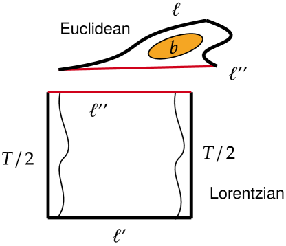
Figure 1: Figure describing the Euclidean and Lorentzian parts of emission of the baby universe.

$$\psi^{\text{disk}}_{\lambda,\beta/2}(\ell)\equiv\langle{\ell}|{HH_{\beta/2,\lambda}}\rangle=\frac{1}{\pi^{2}}\int_{0}^{\infty}dE^{\prime}\sinh(2\pi\sqrt{E^{\prime}})e^{-\frac{\ell}{2}}K_{2i\sqrt{E^{\prime}}}(4e^{-\frac{\ell}{2}})e^{\frac{\beta}{8\lambda}(\sqrt{1-8\lambda E^{\prime}}-1)}\,.$$ (66)

Performing a variable change $E^{\prime}=E(1-2\lambda E)$ we have

$$\psi^{\text{disk}}_{\lambda,\beta/2}(\ell)=\int_{0}^{\infty}dE\rho^{\text{disk}}_{\lambda}(E)e^{-\frac{\beta E}{2}}\left(4e^{-\frac{l}{2}}K_{2i\sqrt{E(1-2\lambda E)}}(4e^{-\frac{l}{2}})\right)$$ (67)

Defining

$$\psi_{E,\lambda}(\ell):=\langle{\ell}|{E}\rangle\equiv 4e^{-\frac{\ell}{2}}K_{2i\sqrt{E(1-2\lambda E)}}(4e^{-\frac{\ell}{2}})\,,$$ (68)

where $|E\rangle$ denotes the bulk eigenstates. The overlap of two Hartle-Hawking wavefunctions for the deformed theory is defined as

$$\langle{HH_{\beta/2}}|{HH_{\beta^{\prime}/2}}\rangle\equiv\int_{-\infty}^{\infty}e^{\ell}d\ell\psi^{*\,\,\text{disk}}_{\lambda,\beta/2}(\ell)\psi^{\text{disk}}_{\lambda,\beta^{\prime}/2}(\ell)\,.$$ (69)

This is consistent with the fact that the norm of the Hartle-Hawking state should be equivalent to the disk partition function given in (20). The normalization of the wavefunction for pure JT gravity in the energy basis is given by,

$$\int_{-\infty}^{\infty}e^{\ell}d\ell\psi_{E}^{*}(\ell)\,\psi_{E^{\prime}}(\ell)=\frac{\delta(E-E^{\prime})}{\rho^{\text{disk}}_{0}(E)}$$ (70)

where $\rho^{\text{disk}}_{0}(E)$ is defined in (19). Similarly, for $T\bar{T}$ case, deformed wavefunctions satisfy the normalization

$$\int_{-\infty}^{\infty}e^{\ell}d\ell\,\psi^{*}_{E,\lambda}(\ell)\psi_{E^{\prime},\lambda}(\ell)=\frac{\delta(E-E^{\prime})}{\rho^{\text{disk}}_{\lambda}(E)},$$ (71)

This expression is essential to evaluate the norm of the Hartle-Hawking wavefunctions.

Trumpet wavefunction and Baby universes:

Figure 2: The growth of ERB length and the emission of baby universes are shown in the figure.

The trumpet wavefunction for pure JT gravity can be expressed in terms of the Hartle-Hawking wavefunction of the disk (in energy basis) as given in Saad:2019pqd . A similar approach can be adopted for the deformed case. The deformed trumpet wavefunction in the length basis is given by,

$$\begin{split}\psi^{\text{trumpet}}_{\beta/2,\lambda}(l,b)=\int_{0}^{\infty}dE\,\rho_{\lambda}^{\text{trumpet}}(b,{E})\,\psi_{E,\lambda}(\ell)e^{-\beta E/2}\,.\end{split}$$ (72)

Now, the propagator in the case of a deformed trumpet can be calculated via the length basis integral decomposition as follows (as described pictorially in Fig. (1)),

$$P_{\text{trumpet}}^{\lambda}(T/2,b,\ell,\ell^{\prime})=e^{-S_{0}}\int_{-\infty}^{\infty}e^{\ell^{\prime\prime}}dl^{\prime\prime}\underbrace{\langle\ell,b|\ell^{\prime\prime}\rangle}_{\textrm{Euclidean part}}\,\,\underbrace{P_{\chi=1}^{\lambda}(T/2,\ell^{\prime\prime},\ell^{\prime})}_{\textrm{Lorentzian part}}$$ (73)

One first writes the propagator as,

$$P_{\text{trumpet}}^{\lambda}(T/2,b,\ell,\ell^{\prime})\sim\langle\ell,b|e^{-i\frac{T}{2}H_{\textrm{bulk}}}|\ell^{\prime}\rangle_{\lambda}\,.$$ (74)

Now we can readily calculate the matrix element in (74) as,

$$\begin{split}\langle\ell,b|e^{-i\frac{T}{2}H_{\textrm{bulk}}}|\ell^{\prime}\rangle_{\lambda}&=\int_{0}^{\infty}dEdE^{\prime}\frac{\langle\ell,b|E^{\prime}\rangle}{\langle E^{\prime}|E^{\prime}\rangle}\langle E^{\prime}|e^{-iT/2H_{\textrm{bulk}}}|E\rangle\frac{\langle E|\ell^{\prime}\rangle}{\langle E|E\rangle}\,,\\ &=\int_{0}^{\infty}dE\,\rho_{\lambda}^{\text{trumpet}}(b,E)e^{-iTE}\psi_{E,\lambda}(\ell)\psi_{E,\lambda}(\ell^{\prime})\,.\end{split}$$ (75)

We change variables from $E(1-2\lambda E)\to E$. Hence, the Lorentzian part of emission probability of the baby universe is given by,

$$\langle\ell,b|e^{-i\frac{T}{2}H_{\textrm{bulk}}}|\ell^{\prime}\rangle_{\lambda}=\int_{0}^{\infty}dE\,\frac{\cos\left(b\sqrt{E}\right)}{2\pi\sqrt{E}}e^{-iTE(\lambda)}\psi_{E}(\ell)\psi_{E}(\ell^{\prime})\,.$$ (76)

We use the following integral representation of the modified Bessel functions,

$$K_{2i\sqrt{E}}\Big{(}4e^{-\ell/2}\Big{)}=\frac{1}{2}\int_{-\infty}^{\infty}dx\,e^{-4e^{-\ell/2}\textrm{{cosh}(x)}}e^{-2ix\sqrt{E}}\,.$$ (77)

Finally, changing the variable to $s=\sqrt{E}$, we can write the amplitude (75) as
gray!12 white

$$\begin{split}\tikzmarkin[disableroundedcorners=true]{re}(0.71,-0.5)(-0.3,1.0)\mathcal{O}(\lambda):\,\,\,\langle\ell,b|e^{-i\frac{T}{2}H_{\textrm{bulk}}}|\ell^{\prime}\rangle_{\lambda}\sim 2iT|\lambda|\,\,e^{\frac{-\ell-\ell^{\prime}}{2}}\int_{-\infty}^{\infty}dx\,dy&e^{-4e^{-\ell/2}\,\textrm{Cosh}(x)-4e^{-\ell^{\prime}/2}\,\textrm{Cosh}(y)}\\ &\times\int_{-\infty}^{\infty}ds\,e^{-is(2x+2y-b)}\,s^{4}\,.\tikzmarkend{re}\end{split}$$ (78)

After evaluating the integral using the saddle point method, we find that, for $T\bar{T}$ deformed case, the emission amplitude increases for the good sign (i.e. negative) of $\lambda$ in the Lorentzian part in (73) (though the Euclidean part $\langle\ell,b|\ell^{\prime\prime}\rangle$ remains the same) when the final length of the ERB is very small (Fig. 2) and both $(\ell,b)\sim\mathcal{O}(1)$ with $\ell^{\prime}\to\infty$. It remains same if we consider $\ell\sim\mathcal{O}(1)$ with $\ell^{\prime}\sim b\to\infty$. In Bhattacharyya:2023gvg , three of the current authors made the following observation after computing the SFF for a deformed JT gravity coupled with $U(1)$ gauge theory: the ramp of the spectral form factor (SFF) of deformed JT gravity ($U(1)$ coupled) grows faster than the undeformed theory, which immediately implies that the possibility of the emission of a single baby universe becomes large (for late times) in the deformed theory. In the context of the present article, we find the same observation holds by directly computing the emission probability (although we only take a $T\bar{T}$ deformation of JT gravity in this paper). Phenomenologically, from these two observations, one can deduce the following: any irrelevant integrable deformation eventually pushes the ramp structure to be faster growing in comparison to the undeformed theory, implying a larger emission amplitude of baby universes.

5 $T\bar{T}$ deformed matrix potential and density correlator

In this section, we find the deformed spectral curve and calculate the deformed matrix potential. The spectral curve of the matrix integral can be written as Saad:2019lba

$$\begin{split}y(E)=-i\pi\rho^{\text{disk}}_{\lambda}(E)\end{split}$$ (79)

where $\rho^{\text{disk}}_{\lambda}(E)$ is the deformed density of states as shown in equation (25), for which the leading order contribution comes from the disk topology. Now, defining the following variable,

$$z^{2}=-E\,.$$ (80)

Hence we have

$$\begin{split}y(z)=(1+4\lambda z^{2})\frac{\sin(2\pi z\sqrt{1+2\lambda z^{2}})}{4\pi}\,.\end{split}$$ (81)

Since it is better to work with determinants instead of resolvents, especially if one wants to consider the non-perturbative effects, we define the following quantity, which we shall refer to as the ‘determinant.’

$$\psi(E)\equiv\text{det}(E-H)e^{-\frac{L}{2}V(E)}\,.$$ (82)

To compute the expectation value $\langle\psi\rangle$ we need to consider an integral over $H$ with a weighting that depends on the deformed matrix potential $V(H,\lambda)$

$$\langle\text{det}(E-H)\rangle=\frac{1}{\mathcal{Z}}\int dH\,\text{det}(E-H)e^{-L\text{Tr}\,V(H,\lambda)}$$ (83)

where the normalization $\mathcal{Z}$ is given by,

$$\mathcal{Z}=\int dH\,e^{-L\text{Tr}\,V(H,\lambda)}\,.$$ (84)

The deformed matrix potential can be calculated using the deformed spectral curve as follows

$$\begin{split}V_{\text{eff}}(E)&=2e^{S_{0}}\int_{0}^{-E}dx\,y(\sqrt{x})\\ &=\frac{e^{S_{0}}}{2\pi}\int_{0}^{-E}dx\,(1+4\lambda x){\sin\big{(}2\pi\sqrt{x(1+2\lambda x)}\big{)}}\,.\end{split}$$ (85)

Changing the variable of integration to $k(x)=\sqrt{x(1+2\lambda x)}$ we have

$$\begin{split}V_{\text{eff}}(E)&=\frac{e^{S_{0}}}{\pi}\int_{0}^{k(-E)}kdk\sin(2\pi k)\\ &=\frac{e^{S_{0}}}{4\pi^{3}}\big{(}\sin[2\pi k(-E)]-2\pi k(-E)\cos[2\pi k(-E)]\big{)}\,.\\ \end{split}$$ (86)

A plot for this effective potential is given in Fig. (3).

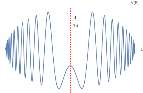
Figure 3: Effective matrix potential for deformed JT gravity with a saddle point at $\frac{1}{4\lambda}$ marked by the dashed line

5.1 Disks and Cylinders

Before proceeding further, we comment on the nature of $V_{\text{eff}}(E)\,.$ For pure JT gravity, the potential is given by

$$V_{\text{eff}}(E)=\frac{e^{S_{0}}}{4\pi^{3}}\Bigg{[}\textrm{sin}(2\pi\sqrt{-E})-2\pi\sqrt{-E}\,\textrm{cos}(2\pi\sqrt{-E})\Bigg{]}\,,\hskip 56.9055ptE<0\,.$$ (87)

As mentioned in Saad:2019lba , this potential is non-perturbatively unstable. After $E=-1/4$, it oscillates rapidly, and it reaches a local maximum at this specific point. One way to get rid of this oscillation is using the ‘one-eigenvalue instantons’ Saad:2019lba . They are sometimes called as ZZ branes. However, they are manifestly different from the FZZT branes, which one can also insert to control these oscillations Saad:2019lba . But for our case, the $T\bar{T}$ deformed matrix potential (LABEL:5.8u) already stops its erratic oscillation near $E\sim\frac{1}{4\lambda}$. It seems that ZZ brane states are natural here. Now, to compute $\langle\psi(E)\rangle$ we use the following identity

$$\text{det}(E-H)=\text{exp}\big{(}\text{Tr}\log(E-H)\big{)}\,.$$ (88)

We can then express the expectation value as follows

$$\begin{split}\langle\text{det}(E-H)\rangle=\text{exp}\bigg{(}\big{\langle}\text{Tr}\log(E-H)\big{\rangle}+\frac{1}{2}\big{\langle}\text{Tr}\log(E-H)\text{Tr}\log(E-H)\big{\rangle}_{\text{conn}}+\cdots\bigg{)}\,.\end{split}$$ (89)

The disk amplitude as a function of $z$ is given below

$$\begin{split}\text{Disk}(z)\equiv e^{S_{0}}\int_{0}^{z}y(z^{\prime})(-2z^{\prime}dz^{\prime})\,.\end{split}$$ (90)

Using the spectral curve for the deformed theory as given in (81), we get,

$$\begin{split}\text{Disk}(z)=\frac{e^{S_{0}}}{4\pi}\int_{0}^{z}(1+4\lambda z^{\prime 2})\sin(2\pi z^{\prime}\sqrt{1+2\lambda z^{\prime 2}})(-2z^{\prime}dz^{\prime})\,.\end{split}$$ (91)

To compute the integral we change the integration variable to $k(z^{\prime})=\sqrt{z^{\prime}(1+2\lambda z^{\prime 2})}$

$$\begin{split}\text{Disk}(z)&=-\frac{e^{S_{0}}}{2\pi}\int_{0}^{k(z)}\sin(2\pi k)kdk\,,\\ &=-\frac{\sin(2\pi k(z))-2\pi k(z)\cos(2\pi k(z))}{8\pi^{3}}e^{S_{0}}\,.\end{split}$$ (92)

The cylinder amplitude is defined as

$$\begin{split}\text{Cyl}(z_{1},z_{2};\lambda)\equiv\int_{\infty}^{z_{1}}(-2z^{\prime}_{1}dz^{\prime}_{1})\int_{\infty}^{z_{2}}(-2z^{\prime}_{2}dz^{\prime}_{2})R_{0,2}(z^{\prime}_{1},z^{\prime}_{2};\lambda)\,.\end{split}$$ (93)

Using the correlator of resolvents as shown in equation (52) , we have

$$\begin{split}\text{Cyl}(z_{1},z_{2};\lambda)&=\int_{\infty}^{z_{1}}(-2z^{\prime}_{1}dz^{\prime}_{1})\int_{\infty}^{z_{2}}(-2z^{\prime}_{2}dz^{\prime}_{2})\left(\frac{1}{4z^{\prime}_{1}z^{\prime}_{2}(z^{\prime}_{1}+z^{\prime}_{2})^{2}}+\frac{\lambda}{4z^{\prime}_{1}z^{\prime}_{2}}\right)\,,\\ &=-\log(z_{1}+z_{2})+\lambda z_{1}z_{2}+\infty\,.\end{split}$$ (94)

Based on the choice of branch, the LHS of equation (89) up to one-loop accuracy can be written in terms of the disk and cylinder amplitudes in the following way,

$$\begin{split}\Psi(z)&=\text{exp}\bigg{[}\text{Disk}(z)+\frac{1}{2}\text{Cyl}(z,z;\lambda)\bigg{]}\,,\\ &=\frac{1}{\sqrt{2z}}\text{exp}\Big{[}\text{Disk}(z)+\frac{\lambda z^{2}}{2}\Big{]}\,.\end{split}$$ (95)

Finally, the density pair correlation function $\langle\rho(E_{1})\rho(E_{2})\rangle$ for $|E_{1}-E_{2}|\ll 1$ and $E_{1},E_{2}>0$ can be computed from the resolvent pair correlator given as

$$\big{\langle}R^{\pm}(E_{1})R^{\pm}(E_{2})\big{\rangle}=\partial_{E_{1}}\partial_{E_{2}}\big{\langle}\psi(E_{1})\psi(E_{2})\tilde{\psi}(E_{1})_{\pm}\tilde{\psi}(E_{2})_{\pm}\big{\rangle}\big{|}_{E_{1}=E_{3},E_{2}=E_{4}}\,.$$ (96)

The density pair correlator can then be found using

$$(-2\pi i)^{2}\langle\rho\rho\rangle=\langle R^{+}R^{+}\rangle+\langle R^{-}R^{-}\rangle-\langle R^{+}R^{-}\rangle-\langle R^{-}R^{+}\,\rangle$$ (97)

We restrict our computation to the terms that are singular as $E_{1}\rightarrow E_{2}$. The one-loop function is given in terms of the disks and cylinders as

$$\begin{split}\Psi(z_{1},z_{2};z_{3},z_{4})=\text{exp}\bigg{[}&\text{Disk}(z_{1})+\text{Disk}(z_{2})-\text{Disk}(z_{3})-\text{Disk}(z_{4})+C(z_{1},z_{3})+C(z_{1},z_{4})\\ &+C(z_{2},z_{3})+C(z_{2},z_{4})-C(z_{1},z_{2})-C(z_{3},z_{4})\bigg{]},\end{split}$$ (98)

where,

$$\begin{split}C(z,z^{\prime})&=\frac{1}{2}\big{(}\text{Cyl}(z,z,\lambda)+\text{Cyl}(z^{\prime},z^{\prime},\lambda)\big{)}-\text{Cyl}(z,z^{\prime},\lambda)\\ &=\log(\frac{z+z^{\prime}}{2\sqrt{zz^{\prime}}})+\frac{\lambda}{2}(z-z^{\prime})^{2}\,.\end{split}$$ (99)

Explicitly $\Psi(z_{1},z_{2};z_{3},z_{4})$ is given as

$$\begin{split}\Psi(z_{1},z_{2};z_{3},z_{4})=\frac{(z_{1}+z_{3})(z_{1}+z_{4})(z_{2}+z_{3})(z_{2}+z_{4})}{4\sqrt{z_{1}z_{2}z_{3}z_{4}}(z_{1}+z_{2})(z_{3}+z_{4})}\text{exp}\bigg{[}\text{Disk}(z_{1})+\text{Disk}(z_{2})-\text{Disk}(z_{3})-\text{Disk}(z_{4})\\ +\frac{\lambda}{2}(z_{1}^{2}+z_{2}^{2}+z_{3}^{2}+z_{4}^{2})-\lambda(z_{1}+z_{2})(z_{3}+z_{4})+\lambda(z_{1}z_{2}+z_{3}z_{4})\bigg{]}\,.\end{split}$$ (100)

The deformed two-point density correlator can then be written following the computations for pure JT gravity as done in Appendix (2) of Saad:2019lba ,

$$\begin{split}\big{\langle}\rho(E_{1})\rho(E_{2})\big{\rangle}\approx&\,\,e^{2S_{0}}\underbrace{\rho_{\lambda}^{\text{disk}}(E_{1})\rho_{\lambda}^{\text{disk}}(E_{2})}_{\text{{\color[rgb]{0,0,0}Semiclassical disconnected piece}}}+e^{S_{0}}\underbrace{\rho_{\lambda}^{\text{disk}}\delta(E_{1}-E_{2})}_{\text{Contact term}}\,\\ &-\underbrace{\frac{1}{2\pi^{2}(E_{1}-E_{2})^{2}}+\frac{e^{-2\lambda(\sqrt{E_{1}}-\sqrt{E_{2}})^{2}}}{2\pi^{2}(E_{1}-E_{2})^{2}}\cos[2\pi e^{S_{0}}\rho_{\lambda}^{\text{disk}}(E_{2})(E_{1}-E_{2})]}_{\text{{\color[rgb]{0,0,0}Modified Non-perturbative contribution at $\mathcal{O}(\lambda)$}}}\,.\end{split}$$ (101)

This is one of the main ingredients required for our subsequent study of the growth of the length of ERB.

Non-perturbative contribution: Alternatively, one can proceed with non-perturbative form of $R^{\lambda}_{0,2}$ and then calculate the two-point density correlator by finding Cyl ($z_{1},z_{2};\lambda$) function analogous to (93) by not expanding it in terms of $\lambda\,.$ Now, we proceed to calculate the deformed matrix elements for $T\bar{T}$ deformed case.

5.2 Deformed matrix elements

We now have all the ingredients needed to calculate the deformed matrix elements corresponding to the non-spinning operator insertion at the boundary. Following Saad:2019pqd , one can identify the deformed matrix element. For the undeformed case,

$$\begin{split}\int_{-\infty}^{\infty}d\ell\,\psi_{E}(\ell)\psi_{E^{\prime}}(\ell)\,e^{-\Delta\ell}=&\frac{|\Gamma(\Delta+(is_{1}+is_{2}))\Gamma(\Delta+(is_{1}-is_{2}))|^{2}}{2^{2\Delta+1}\Gamma(2\Delta)},\hskip 17.07182pt\text{with }s_{1}=\sqrt{E},s_{2}=\sqrt{E^{\prime}}\\ &=\mathcal{M}_{\Delta}(E,E^{\prime})\,.\end{split}$$ (102)

Similarly, for the deformed case :

$$\begin{split}\int_{-\infty}^{\infty}d\ell\,\psi_{E}^{\lambda}(\ell)\psi_{E^{\prime}}^{\lambda}(\ell)\,e^{-\Delta\ell}&=\frac{\left|\Gamma\left(\Delta+(i\sqrt{s_{1}^{2}(1-2\lambda s_{1}^{2})}\pm i\sqrt{s_{2}^{2}(1-2\lambda s_{2}^{2})})\right)\right|^{2}}{2^{2\Delta+1}\Gamma(2\Delta)}\\ &=\mathcal{M}_{\Delta}^{\lambda}(E,E^{\prime})\,.\end{split}$$ (103)

Where we used the notation $\Gamma(\Delta+(a\pm b))=\Gamma(\Delta+(a+b))\Gamma(\Delta+(a-b))$. Now, we proceed to calculate the expectation of the length or one-point function $\langle\ell(t)\rangle$. First, we will study it by considering the contribution only from geometries that do not have any genus. Then, we can start using cutting and bootstrapping techniques to use the lower building blocks to produce the expectation of length, taking into account the contribution of geometries with genus Iliesiu:2021ari .

6 Expectation of ERB length

Following the arguments in Iliesiu:2021ari , the length of the ERB is defined as,

$$\langle\ell\rangle=\lim_{\Delta\rightarrow 0}\left\langle\sum_{\gamma}\ell_{\gamma}e^{-\Delta\ell_{\gamma}}\right\rangle$$ (104)

where $\gamma$ labels the non-self-intersecting geodesics, $\langle\cdots\rangle$ represents summing over surfaces of arbitrary topologies while evaluating the gravitational path integral and $\Delta$ acts as a regulator. This definition of length can be related to the two-point function $\langle\chi\chi\rangle$ of the operator of conformal dimension $\Delta$ inserted on each side of the two-sided black hole. We do not have to worry about divergences in this quantity since the time-dependent piece that we are interested in is finite Iliesiu:2021ari . Hence, we study the quantity $\langle\ell(t)\rangle-\langle\ell(0)\rangle$, which is independent of the regularization procedure. $\langle\ell(t)\rangle$ can be computed by taking the $\Delta$ derivative of the two-sided correlation function as given below:

$$\langle\ell(t)\rangle=-\lim_{\Delta\rightarrow 0}\frac{\partial}{\partial\Delta}\big{\langle}\chi_{L}(t)\chi_{R}(0)\big{\rangle}_{\text{non-int}}\,.$$ (105)

In JT gravity, the integral over all metrics reduces to an integral over the boundary wiggles with measure $\mathcal{D}(\mathcal{W})$. The two-point function then can be cast as Iliesiu:2021ari ,

$$Tr_{\beta}\langle\chi(x_{1})\chi(x_{2})\rangle_{\textrm{non-int}}=\sum_{g}e^{S_{0}(1-2g)}\int_{\frac{\mathcal{T}_{g,1}}{Mod(\mathcal{M}_{g,1})}}\omega\int\mathcal{D}(\mathcal{W})\,e^{-I_{JT},bdy(\mathcal{W})}\sum_{\gamma}e^{-\Delta l_{\gamma}}$$ (106)

where

$$\omega=\sum_{j=1}^{3g-3+n}db\wedge d\tau$$

is the usual Weil-Peterson symplectic form defined on the moduli space of hyperbolic Riemann surface. Using the same analogy for $T\bar{T}$ deformed theory, the trumpet wavefunction in terms of $\psi_{E,\lambda}(\ell)$, with a geodesic of length $\ell$ can be written as,

$$\psi^{\textrm{trumpet},x}_{\lambda}(\ell,b)=\begin{minipage}[h]{65.04034pt} \vskip-2.84544pt \scalebox{1.3}{\includegraphics[width=433.62pt]{Trumpet_x.png}} \end{minipage}\hskip 22.76228pt=\int_{0}^{\infty}dE\rho^{\textrm{trumpet}}_{\lambda}(b,E)\psi_{E,\lambda}(\ell)\,e^{-xE},$$ (107)

where,

$$\rho_{\lambda}^{\text{trumpet}}(b,E)=(1-4\lambda E)\frac{\cos\left(b\sqrt{E(1-2\lambda E)}\right)}{2\pi\sqrt{E(1-2\lambda E)}}$$ (108)

is the deformed trumpet density of states. Now, the genus-g contribution can be written compactly as,

$$\begin{split}Tr_{\beta}(\chi(x_{1})\chi(x_{2}))\rangle_{\textrm{non-int}}&\sim e^{S_{0}(1-2g)}\int_{-\infty}^{\infty}d\ell\,e^{\ell}\int_{0}^{\infty}db_{1}b_{1}db_{2}b_{2}\psi^{\textrm{trumpet},x}_{\lambda}(\ell,b_{1})\psi^{\textrm{trumpet},\beta-x}_{\lambda}(\ell,b_{2})e^{-\Delta\ell}\\ &\times\Bigg{[}\textrm{Vol}_{g-1,2}(b_{1},b_{2})+\sum_{h\geq 0}\textrm{Vol}_{g-h,1}(b_{1})\textrm{Vol}_{h,1}(b_{2})\Bigg{]}\,.\end{split}$$ (109)

Therefore, the two-point function for the $T\bar{T}$ deformed theory can be written in terms of the two-point density correlator and the squared matrix element of operator insertions as,

$$\begin{split}\big{\langle}\text{Tr}_{\beta}(\chi(x_{1})\chi(x_{2}))\big{\rangle}_{\text{non-int.}}=\frac{4e^{-S_{0}}}{Z_{\lambda}^{\text{disk}}(\beta)}\int_{0}^{\infty}dE_{1}dE_{2}\big{\langle}\rho(E_{1})\rho(E_{2})\big{\rangle}_{\lambda}e^{-E_{1}(x_{1}-x_{2})-E_{2}(\beta-x_{1}+x_{2})}\mathcal{M}^{\lambda}_{\Delta}(E_{1},E_{2})\end{split}$$ (110)

where $\mathcal{M}^{\lambda}_{\Delta}(E_{1},E_{2})$ takes the form given in equation (103) with $s_{1,2}\equiv\sqrt{E_{1,2}}$. Since there is a unique geodesic for a disk, we see if $\langle\chi(x_{1})\chi(x_{2})\rangle_{\text{non-int.}}^{\Delta\rightarrow 0}=1$ at the leading order as a consistency check. We have,

$$\begin{split}\mathcal{M}_{0}^{\lambda}(s_{1},s_{2})&=\frac{\delta\left(s_{1}-s_{2}\right)}{4(1-4\lambda s_{1}^{2})\,r\left(\sqrt{s_{1}^{2}(1-2\lambda s_{1}^{2})}+\sqrt{s_{2}^{2}(1-2\lambda s_{2}^{2})}\right)},\,\,\hskip 28.45274ptr(s)=\frac{s}{2\pi^{2}}\sinh(2\pi s)\,.\end{split}$$ (111)

Here, we have used the following properties of gamma functions

$$|\Gamma(bi)|^{2}=\frac{\pi}{b\sinh(\pi b)}\hskip 14.22636pt;\hskip 14.22636pt{\bf B(z,-z)}=\lim_{\epsilon\rightarrow 0}\frac{\Gamma(z)\Gamma(-z)}{\Gamma(\epsilon)}=2\pi\delta(z)$$ (112)

where ${\bf B(x,y)}$ is the beta function. Hence we have

$$\begin{split}\big{\langle}\chi(x_{1})\chi(x_{2})\big{\rangle}_{\text{non-int.}}^{\Delta\rightarrow 0}\big{|}_{\text{LO}}&=\frac{4e^{-S_{0}}}{Z_{\lambda}^{\text{disk}}(\beta)}\int_{0}^{\infty}ds_{1}\,ds_{2}\,4s_{1}s_{2}\rho_{\lambda}^{\text{disk}}(s_{1}^{2})\rho_{\lambda}^{\text{disk}}(s_{2}^{2})e^{-(s_{1}^{2}(x_{1}-x_{2})+s_{2}^{2}(\beta-x_{1}+x_{2}))}\mathcal{M}^{\lambda}_{0}(s_{1},s_{2})\,\\ &=\frac{1}{Z_{\lambda}^{\text{disk}}(\beta)}\int_{0}^{\infty}ds_{1}2s_{1}\rho_{\lambda}^{\text{disk}}(s_{1}^{2})e^{-\beta s_{1}^{2}}=1\,.\end{split}$$ (113)

We perform this to verify the matrix element we found in (103). Now, we discuss the growth rate of the Einstein-Rosen bridge (ERB). This can be calculated from the one-point function of $\ell(t)$ in the deformed theory. We also study the saturation of the interior growth in $T\bar{T}$ deformed setup by using the non-perturbative kernel and $T\bar{T}$ deformed matrix element.

Time-dependence of ERB length

We study the time dependence of the length of the Einstein-Rosen bridge using the following relation,

$$\big{\langle}\ell(t)\big{\rangle}\equiv\big{\langle}\text{Tr}_{\beta}(\hat{\ell})\big{\rangle}\equiv-\lim_{\Delta\rightarrow 0}\frac{\partial\left\langle\text{Tr}_{\beta}\left(\chi(\frac{\beta}{2}+it)\chi(0)\right)\right\rangle_{\text{non-int}}}{\partial\Delta}\,.$$ (114)

We define,

$$\omega\equiv s_{1}-s_{2}\,\,\text{ and }\,\,\,\,\,\bar{s}=\frac{s_{1}+s_{2}}{2}$$ (115)

From (110) we can see that the only $\Delta$ dependent term in the two-point function is $\mathcal{M}_{\Delta}^{\lambda}$, hence we take the derivative inside the integral:

$$\begin{split}-\lim_{\Delta\rightarrow 0}\frac{\partial\mathcal{M}_{\Delta}^{\lambda}}{\partial\Delta}=\#\delta(\omega)-\frac{1}{16\pi^{2}\,r(\bar{s})\,r(\frac{\omega}{2})}\,.\end{split}$$ (116)

Since $\#\delta(\omega)$ only gives a time-independent contribution, the expression for length becomes,

$$\begin{split}\big{\langle}\ell(t)\big{\rangle}_{\lambda}=\text{const}-\frac{e^{-S_{0}}}{4\pi^{2}Z_{\lambda}^{\text{disk}}(\beta)}\int_{0}^{\infty}ds_{1}ds_{2}\,s_{1}s_{2}\frac{\big{\langle}\rho(s_{1})\rho(s_{2})\big{\rangle}_{\lambda}}{r(\bar{s})r(\frac{\omega}{2})}\,\,\text{exp}\left[-\beta\left({\bar{s}^{2}}+\frac{\omega^{2}}{4}\right)-i\bar{s}\omega t\right]\\ \,\end{split}$$ (117)

where $\big{\langle}\rho(s_{1})\rho(s_{2})\big{\rangle}_{\lambda}$ is the $T\bar{T}$ deformed correlator and takes the form as given in (101). The contact term gives a time-independent contribution to the integral and hence can be omitted. To perform the integral in (LABEL:5.8ke), we first perform the integral over $\omega$ and then integrate the remaining integrand asymptotically. In the limit $|s_{1}-s_{2}|<<1$ we can write (LABEL:5.8ke) as,

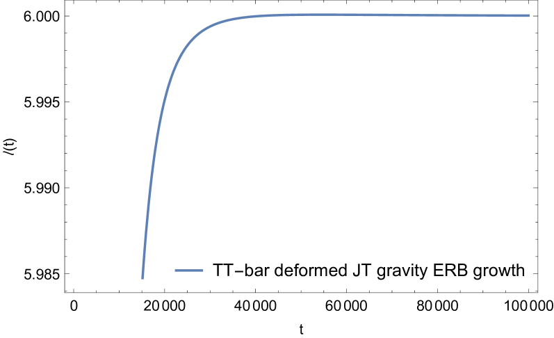
Figure 4: The growth and saturation of ERB length for $T\bar{T}$ deformed theory.

The $\omega$ integral: We are mainly interested in large time regime ($t>t_{*}$). Therefore, $\exp[-i\bar{s}\omega t]$ will be dominated by $\omega\sim 1/t$ and we can implement this by scaling $\omega=\frac{\hat{\omega}}{t}$. Now, the $\omega$ integral becomes ,

$$\begin{split}\mathscr{I}(s)=\mathcal{N}t\int_{-\infty}^{\infty}d\hat{\omega}\,e^{-is\hat{\omega}}\frac{x}{\hat{\omega}^{2}}\Bigg{[}{\color[rgb]{0,0,0}1}-{\color[rgb]{0,0,0}{\frac{t^{2}}{8\pi^{2}\hat{\rho}^{2}\hat{\omega}^{2}s^{2}}+\frac{t^{2}e^{-2\lambda\omega^{2}}}{8\pi^{2}\hat{\omega}^{2}s^{2}\hat{\rho}^{2}}\textrm{cos}\Bigg{(}\frac{4\pi\hat{\rho}\hat{\omega}s}{t}\Bigg{)}}}\Bigg{]}\end{split}$$ (118)

where,

$$x=-8\pi^{3}\text{csch}(2\pi s)\left(2\pi\lambda s^{3}\coth(2\pi s)+7\lambda s^{2}-1\right)\,.$$ (119)

In (118), the first term in the parenthesis comes from the semiclassical disconnected part, and the rest of the terms come from the non-perturbative contribution. After performing this Fourier transform, and using the notation $\rho_{\lambda}(s)=e^{S_{0}}\hat{\rho}_{\lambda}(s)\text{ and }\,\,t=e^{S_{0}}\hat{t}$, we get,

$$\begin{split}\mathscr{I}(s)=&384\pi^{5}\sqrt{2}\lambda\hat{\rho}_{\lambda}(s)^{4}s^{7}(2\pi s\coth(2\pi s)+7)-384\pi^{5}\sqrt{2}\hat{\rho}_{\lambda}(s)^{4}s^{5}-128\pi^{3/2}\sqrt{\lambda}\hat{\rho}_{\lambda}(s)s^{2}t^{2}e^{-\frac{\left(64\pi^{2}\hat{\rho}_{\lambda}(s)^{2}+1\right)s^{2}}{8\lambda}}\\ &\sinh\left(2\pi\hat{\rho}_{\lambda}(s)s^{2}/\lambda\right)+8\sqrt{\pi}\sqrt{\lambda}\left(64\pi^{2}\hat{\rho}_{\lambda}(s)^{2}+1\right)s^{2}t^{2}e^{-\frac{\left(64\pi^{2}\hat{\rho}_{\lambda}(s)^{2}+1\right)s^{2}}{8\lambda}}\cosh\left(2\pi\hat{\rho}_{\lambda}(s)s^{2}/\lambda\right)\\ &-4\sqrt{\pi}\sqrt{\lambda}(8\pi\hat{\rho}_{\lambda}(s)+1)^{2}s^{2}t^{2}e^{-\frac{(8\pi\hat{\rho}_{\lambda}(s)s+s)^{2}}{8\lambda}}-4\sqrt{\pi}\sqrt{\lambda}(1-8\pi\hat{\rho}_{\lambda}(s))^{2}s^{2}t^{2}e^{-\frac{(1-8\pi\hat{\rho}_{\lambda}(s))^{2}s^{2}}{8\lambda}}\\ &-\sqrt{2}\pi st^{2}\Big{(}(1-8\pi\hat{\rho}_{\lambda}(s))^{3}\left(-s^{2}\right)+2s^{2}-{(8\pi\hat{\rho}_{\lambda}(s)+1)}s^{2}(8\pi\hat{\rho}_{\lambda}(s)+1)^{2}\Big{)}\\ &+\sqrt{2}\lambda t^{2}\Big{(}\pi s^{3}\Big{[}(1-8\pi\hat{\rho}_{\lambda}(s))^{3}\left(-s^{2}\right)+2s^{2}\\ &-{(8\pi\hat{\rho}_{\lambda}(s)+1)}s^{2}(8\pi\rho_{\lambda}(s)+1)^{2}(2\pi s\coth(2\pi s)+7)\Big{]}+12\pi\left(16\pi\hat{\rho}_{\lambda}(s)\right)s\Big{)}\,.\end{split}$$ (120)

Since this function is very complicated, one can only perform it numerically. However, if we want to compute the ERB length at a large time, then analytical computation is possible. Hence, the remaining $s$ integral can be performed, and we get,

$$\begin{split}\big{\langle}\ell(\hat{t})\big{\rangle}_{\lambda}&=\text{const}-\frac{\hat{t}e^{S_{0}}}{4\pi^{2}Z_{\lambda}^{\text{disk}}(\beta)}\int_{0}^{\infty}d{s}\,{s}^{2}\,{\hat{\rho}_{\lambda}(s)^{2}}\times\,\mathscr{I}({s})e^{-\beta s^{2}}\,.\end{split}$$ (121)

One can check that $\textrm{erf}(t^{2})\approx 1-\frac{e^{-t^{4}}}{\sqrt{\pi}t^{2}}$. So the leading order term at large $t$ is given by,

$$\begin{split}\big{\langle}\ell(\hat{t})\big{\rangle}_{\lambda}&=\text{const}+\frac{\hat{t}^{3}e^{3S_{0}}}{4\pi^{2}Z_{\lambda}^{\text{disk}}(\beta)}\int_{s_{*}(\hat{t})}^{\infty}ds\,{\hat{\rho}_{\lambda}(s)^{2}}s^{2}\\ &\times\Bigg{(}-\frac{4\sqrt{2}\pi^{3/2}e^{\beta\left(-s^{2}\right)}\text{csch}(2\pi s)\left(2\pi\lambda s^{3}\coth(2\pi s)+7\lambda s^{2}-1\right)}{s^{2}\hat{\rho}_{\lambda}^{2}(s)}\Bigg{)}.\end{split}$$ (122)

Here $s_{*}(t)$ is fixed from the equation, $\hat{t}=\pi\,\frac{\hat{\rho}_{\lambda}(s_{*}(\hat{t}))}{1+4\lambda s_{*}(\hat{t})^{2}}$ . Now we try to solve for $s_{*}(t)$ and get the following,

$$s_{*}(\hat{t})=\frac{1}{2\sqrt{\pi\lambda}}\left(\pi-\sqrt{\pi^{2}-2\lambda\sinh^{-1}\left(\frac{\hat{t}}{2\pi}\right)^{2}}\right)^{\frac{1}{2}}\,.$$ (123)

Hence, after performing the integral asymptotically, i.e. replacing the $sinh$ functions by exponential and considering, we get

gray!12 white

$$\begin{split}\tikzmarkin[disableroundedcorners=true]{kol}(4.1,-1.08)(-0.8,1.2)\hskip-19.91684pt\big{\langle}\ell(t)\big{\rangle}_{\mathcal{O}({\lambda})}\approx&\text{Const.}-e^{S_{0}}\hat{t}^{2}\frac{\exp\left(-\frac{\pi^{2}\left(\beta^{2}+2\pi^{2}\lambda\right)}{\beta^{3}}-\frac{\log^{2}(\hat{t})\left(2\pi^{2}\beta+\lambda\log(\hat{t})\left(\beta\log(t)+2\pi^{2}\right)\right)}{8\pi^{4}}\right)}{\sqrt{2}\pi^{7/2}\beta^{2}}\\ &\times\Bigg{[}\Big{(}-e^{\frac{\left(\frac{\beta\log(\hat{t})}{2\pi}+\pi\right)^{2}}{\beta}}\text{erfc}\left(\frac{\beta\log(\hat{t})+2\pi^{2}}{2\pi\sqrt{\beta}}\right)\Big{(}8\pi^{4}\Big{(}\beta^{3}-11\beta^{2}\lambda-14\pi^{2}\beta\lambda+2\pi^{4}\lambda)\Big{)}\\ &+\beta^{3}\lambda\log^{3}(\hat{t})\left(\beta\log(\hat{t})+2\pi^{2}\right)\Big{)}+2\sqrt{\pi}\sqrt{\beta}\lambda\Big{(}-20\pi^{4}\beta\\ &+\beta\log(\hat{t})(14\pi^{2}\beta+\beta\log(t)\left(\beta\log(\hat{t})+2\pi^{2}\right)-4\pi^{4})+8\pi^{6}\Big{)}\Bigg{]}\,.\tikzmarkend{kol}\end{split}$$ (124)

We found that the length growth for the $T\bar{T}$ deformed theory has a faster saturation than the undeformed theory, as shown in Fig. (4). A comparison between the plots for the two cases is given in Fig. (5). This also supports the calculation of the emission probability of the baby universes. In this case, the emission probability increases because of the $T\bar{T}$ deformation. As a physical description of the event, as the probability of the baby universe emission increases due to such an irrelevant deformation, the ERB length decreases faster after deformation and gives a non-trivial overlap with the dual Hartle-Hawking initial state of fixed length.

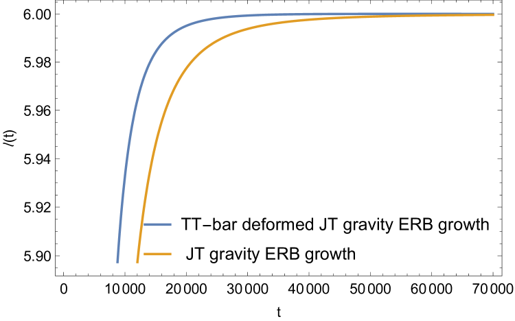
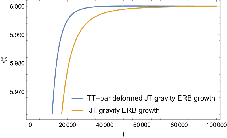
Figure 5: Plots showing the growth of the ERB for JT gravity and $T\bar{T}$ deformed JT gravity

A possible connection with Krylov complexity As the length of ERB saturates for the $T\bar{T}$ deformed theory, similar to JT gravity, it is natural to expect some connection with Krylov complexity following Kar:2021nbm ; Balasubramanian:2024lqk . The Krylov complexity of an operator $\mathcal{O}(t)$ is given by PhysRevX.9.041017 ,

$$C_{E}(t)=\sum_{n=0}^{D(E)}n|\phi_{E,n}(t)|^{2}$$ (125)

with $D(E)$ is the dimension of the Krylov space. Now the $\phi_{E,n}(t)s$ can be found by solving the following discrete Schrodinger equation in the Krylov basis,

$$\dot{\phi}_{E,n}(t)=b^{E}_{n+1}\phi_{E,n+1}(t)-b^{E}_{n}\phi_{E,n-1}(t)$$ (126)

where, $b^{E}_{n}$ are the Lanczos coefficients viswanath1994recursion . This exact equation is valid in any quantum state. Hence, we proceed to compute the K-complexity initial growth using the moment method as follows. The deformed matrix element for our case with $s_{1}=\sqrt{E_{1}},\,s_{2}=\sqrt{E_{2}}$ is given by,

$$\begin{split}\mathcal{M}_{\Delta}^{\lambda}(E,E^{\prime})&=\frac{\left|\Gamma\left(\Delta+(i\sqrt{E_{1}(1-2\lambda E_{1})}\pm i\sqrt{E_{2}(1-2\lambda E_{2})})\right)\right|^{2}}{2^{2\Delta+1}\Gamma(2\Delta)}\,.\end{split}$$ (127)

Now, at the leading order of the two-point correlator (the disconnected piece is enough for showing the growth), $\langle\rho\rho\rangle$ is given by,

$$\begin{split}\rho_{\textrm{def}}(E,\omega)=\rho_{\lambda}\left(E+\frac{\omega}{2}\right)\rho_{\lambda}\left(E-\frac{\omega}{2}\right),\,\omega=E_{1}-E_{2},\,E=\frac{E_{1}+E_{2}}{2}\,.\end{split}$$ (128)

Explicitly, it takes the following form,

$$\begin{split}\rho_{\textrm{def}}(E,\omega)=\frac{1}{4\pi^{2}}\left(1-4\lambda\left(E+\frac{\omega}{2}\right)\right)\sinh\left[2\pi\sqrt{\left(E+\frac{\omega}{2}\right)\left(1-2\lambda\left(E+\frac{\omega}{2}\right)\right)}\right]\times(\omega\to-\omega)\,.\end{split}$$ (129)

Focusing on the small moments, one can approximate the two-point correlator as,

$$\begin{split}\rho_{\textrm{def}}(E,\omega)\to(1-8\lambda E)\exp\left(4\pi\sqrt{{E}(1-2{E}\lambda)}\right)\end{split}$$ (130)

and,

$$\begin{split}\mathcal{M}_{\Delta}^{\lambda}(E,\omega)\xrightarrow[]{}\frac{\left|\Gamma\left(\Delta+i\left(2\sqrt{E(1-2E\lambda)}+\mathcal{O}(\frac{\omega^{2}}{E^{2}})\right)\right)\Gamma\left(\Delta+i\left(\frac{(1-4\lambda E)}{\sqrt{1-2E\lambda}}\right)\frac{\omega}{2\sqrt{E}}+\mathcal{O}(\omega^{2}/E^{3/2})\right)\right|^{2}}{2^{2\Delta+1}\Gamma(2\Delta)}.\end{split}$$ (131)

Now using the following identity Kar:2021nbm ,

$$|\Gamma(\Delta+ir)|^{2}=\frac{\pi r}{\sinh(\pi r)}\prod_{k=1}^{\Delta-1}(r^{2}+k^{2}),$$ (132)

we can write the matrix element as,

$$\begin{split}\mathcal{M}_{\Delta}^{\lambda}(E,\omega)&\xrightarrow[]{}\frac{1}{\sinh\left(2\pi\sqrt{E(1-2E\lambda)}\right)\sinh\left(\pi\frac{(1-4\lambda E)}{\sqrt{1-2E\lambda}}\frac{\omega}{2\sqrt{E}}\right)}\\ &\sim\exp\left(S(E)-\frac{\beta_{E}\omega}{2}\right),\end{split}$$ (133)

where,

$$S(E)=2\pi\sqrt{E(1-2E\lambda)},\,\,\beta_{E}=\pi\frac{1-4\lambda E}{\sqrt{E(1-2E\lambda)}}\equiv\frac{\partial S(E)}{\partial E}\,.$$ (134)

The average energy moments are given by Kar:2021nbm ,

$$\begin{split}m_{2n}^{E}&\xrightarrow[]{}\frac{1}{\mathcal{N}(E)}\int_{-2E}^{2E}d\omega\,\omega^{2n}\rho_{\textrm{def}}(E,\omega)\,\mathcal{M}_{\Delta}^{\lambda}(E,\omega)\,,\\ &=\frac{1}{\int_{-2E}^{2E}d\omega\,\exp\left(-\beta_{E}\omega/2\right)}\int_{-2E}^{2E}d\omega\,e^{2n\log\omega}\exp\left(-\frac{\beta_{E}\omega}{2}\right)\,.\end{split}$$ (135)

One can do the integral using the saddle point approximation, which is valid in the parametric region $\beta_{E}^{-1}\ll\omega\ll E$. The saddle point condition reads,

$$\frac{2n}{\omega_{*}}=\frac{\beta_{E}}{2}\implies\omega_{*}=\frac{4n}{\beta_{E}}\,.$$ (136)

Therefore, the moments become,

$$\begin{split}m_{2n}^{E}=\frac{1}{\mathcal{N}(E)}\left(\frac{4n}{\beta_{E}}\right)^{2n}e^{-2n+\cdots}\to e^{n\left(\log(4n/\beta_{E})^{2}-2\right)}\end{split}$$ (137)

For large $n$ we can approximate it to,

$$m_{2n}^{E}\sim e^{n[\log(4n/\beta_{E})]^{2}}\,.$$ (138)

Therefore, the Lanczos coefficient is given by,

$$b_{n}^{E}\sim\frac{n}{\beta_{E}},\,\,\,\,\beta_{E}=\pi\frac{1-4\lambda E}{\sqrt{E(1-2E\lambda)}}\,.$$ (139)

Following Kar:2021nbm , using the definition of Krylov complexity (125) we have,

$$C_{E}(t)\sim e^{\frac{2\pi}{\beta_{E}}t}=\exp\left(2t\frac{\sqrt{E(1-2E\lambda)}}{1-4\lambda E}\right),\,\quad t\lesssim\beta_{E}\log(S(E))\,.$$ (140)

For the good sign of $\lambda$, one can see that, at initial times, Krylov complexity grows faster in JT gravity compared to the deformed theory. Now, if we assume that the proposal relating Krylov complexity with that of the ERB length $\langle\ell(t)\rangle\sim C_{E}(t)$ Rabinovici:2023yex ; Balasubramanian:2024lqk ; Heller:2024ldz ; Ambrosini:2024sre , is also valid at early times, then we can claim that $\langle\ell(t)\rangle$ should grow faster in the undeformed theory. However, at late times, we have seen that $\langle\ell(t)\rangle$ saturates faster for the deformed theory. Hence, one can expect that in the intermediate time, there must be a crossover. However, to check it concretely, one needs to do the computations from both sides for the entire range of the time, which we shall leave for further investigation.

7 Conclusion and Discussion

Motivated by the interesting aspects of $T\bar{T}$ deformation, we discuss the emission probability of baby universes after applying such an integrable irrelevant deformation. We also computed the ERB length growth after $T\bar{T}$ deformation and found interesting results that agree with our previous paper Bhattacharyya:2023gvg . We also comment and explicitly show the computation of the deformed Kernel, which encodes the non-perturbative corrections. Below, we list the main findings of our paper,

1. We compute the deformed resolvents and spectral curve and determine the dual matrix model potential for $T\bar{T}$ deformed JT gravity. While finding the matrix potential for our model, we found that even without adding any instanton corrections, the nature of the potential is such that it leads to less oscillation automatically at some specific value of the energy depending on the value of the deformation parameter and this has a deep connection to eigenvalue repulsion leading to the promisingly different behaviour of the SFF or other quantities like ERB growth, which is worth investigating. We also comment on the possible connection of Krylov complexity with the growth of the black hole interior. For that case, to obtain an analytic handle, we only focused on the early time behavior, leaving the detailed study for the future..

2. The emission probability of baby universes increases, leading to a higher slope and non-linear ramp, as predicted in our earlier paper Bhattacharyya:2023gvg . One should note that the probability of the emission increases for a good sign of the deformation parameter, i.e. $\lambda<0$, and it is very sensitive to the sign of $\lambda$.

3. We calculate the growth rate of the ERB for late times. Though the classical prediction says that the complexity should increase linearly in time, non-perturbative quantum corrections lead to the saturation of the complexity in JT gravity. Interestingly, we found that after applying $T\bar{T}$ deformation, the saturation becomes faster. The volume growth stops earlier than pure JT gravity.

4. In Appendix (A), we also compute the correction to the moduli space volume arising due to the change in the spectral curve because of the $T\bar{T}$ deformation. We attempt to find the moduli space volume by taking $\mathcal{O}(\lambda)$ correction to $R_{T}\,$. We find that due to the presence of the deformation, there is a non-trivial branch cut in the $z-$plane. We only consider the physical poles contributing to the inverse Laplace integral. Finally, we show that switching off the deformation would lead to the original volume without the finite cutoff. We also comment on why the volume of the moduli space should change even if we consider a boundary deformation.

Now, we end this section by discussing some possible future outlooks. It is known that the $T\bar{T}$ deformation affects the high energy levels in a non-trivial way. Due to this irrelevant deformation, the ultraviolet behaviour of the theory changes. One interesting extension would be to check the ERB length growth for flat space BMS Schwarzian. The other quick extension is to calculate the variance of the length in the presence of the $T\bar{T}$ deformed theory and check at which scale the oscillation starts about the plateau. One can also try to generalize this computation for self-intersecting geodesics. As it is still not clearly understood what sort of geometries affect the complexity and lead to the saturation of the interior volume, it is a very interesting direction to analyze even in the absence of $T\bar{T}$ deformation.

Appendix A $T\bar{T}$ deformation of the volume of moduli space

We begin by introducing the spectral curve. We define the following curve,

$$E(z)=-z^{2}\,.$$

In order to find the resolvents for the trumpet partition function, we do the following integral transform Stanford:2019vob ,

$$\begin{split}R_{T}&=-\int_{0}^{\infty}d\beta e^{-\beta z^{2}}Z_{trumpet}^{\lambda}(\beta,b)\,,\\ &=\frac{1}{2}\,\lambda\,z\,e^{-bz}(bz-3)-\frac{e^{-bz}}{2z},\,\quad\lambda<0\,.\end{split}$$ (141)

Now, the resolvents can be written in terms of moduli space volumes as follows Stanford:2019vob ,

$$R_{g}(-z_{1}^{2},\cdots,-z_{n}^{2})=\int_{0}^{\infty}V_{g}(b_{1},\cdots b_{n})\prod_{j=1}^{n}b_{j}db_{j}\,R_{T}(b_{j},z_{j};\lambda)\,.$$ (142)

Hence, we can write the deformed volume as

$$V_{g}(b_{1},\cdots b_{n})_{\lambda}=\int_{c_{0}+i\mathbb{R}}R_{g}^{\lambda}(-z_{1}^{2},\cdots,-z_{n}^{2})\prod_{j=1}^{n}\frac{dz_{j}}{2\pi i}\,\,\frac{1}{R_{T}(b_{j},z_{j};\lambda)b_{j}}$$ (143)

For our case, we specifically compute the following,

$$V_{1}(b_{1})_{\lambda}=\int_{c_{0}+i\mathbb{R}}\,\,\frac{dz}{2\pi i}\,\,\frac{1}{R_{T}(b,z;\lambda)b}\,\,R_{1}^{\lambda}(-z^{2})\,.$$ (144)

Now we can define

$$\begin{split}&W_{g,n}(z-1,z_{2},\cdots,z_{n};\lambda)=\textrm{Res}_{z\rightarrow 0}\mathcal{K}(z_{1},z;\lambda)\Bigg{[}W_{g-1,n+1}(z,-z,z_{2}\cdots,z_{n};\lambda)+\\ &\hskip 256.0748pt\sum_{\begin{subarray}{c}h_{1}+h_{2}=g\\ I_{1}\bigcup I_{2}=J\end{subarray}}^{*}W_{h_{1},1+|I_{1}|}(z,I_{1},\lambda)\,\,W_{h_{2},1+|I_{2}|}(-z,I_{2},\lambda)\Bigg{]}\,\end{split}$$ (145)

Here the ‘*’ indicates that one should not consider cases when $\{h_{2},I_{2}\}\mbox{ or }\{h_{1},I_{1}\}=\{g,J\}$. The kernel is given by the following expression,

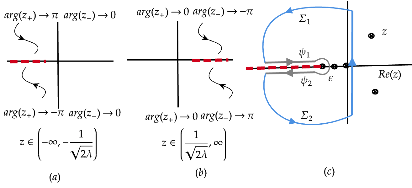
Figure 6: Contour for the integral to find the moduli space volume in $T\bar{T}$ deformed case ($z_{+}=z+\frac{1}{\sqrt{2\lambda}},\,\,z_{-}=\frac{1}{\sqrt{2\lambda}}-z$).

$$\begin{split}\mathcal{K}(z_{1},z;\lambda)&=\frac{1}{2[W_{0,1}(z;\lambda)+W_{0,1}(-z,\lambda)]}\int_{-z}^{z}dz_{2}W_{0,2}(z_{1},z_{2},\lambda)\\ &=\frac{(2+\lambda z_{1}^{2})\sqrt{4+\lambda z^{2}}}{(2+\lambda z^{2})\sqrt{4+\lambda z_{1}^{2}}}\frac{4\pi\textrm{ cosec}(\pi z\sqrt{4+\lambda z^{2}})}{(z_{1}^{2}-z^{2})[4+\lambda(z_{1}^{2}+z^{2})]}\,.\end{split}$$ (146)

Now, by change of variables $R_{g,n}$’s are related with $W_{g,n}$’s in the following way Mirzakhani:2011gta ; Mirzakhani:2006eta ,

$$W_{g,n}(z_{1},z_{2},\cdots z_{n};\lambda)=R_{g,n}(E(z_{1}),\cdots,E(z_{n});\lambda)\,\,E^{\prime}(z_{1})\cdots E^{\prime}(z_{n})\,.$$ (147)

Now following Griguolo:2021wgy ,

$$W_{1,1}(z_{1},\lambda)=\frac{(2+8\lambda z_{1}^{2})[6+\pi^{2}z_{1}^{2}(4+8\lambda z_{1}^{2})]}{3z_{1}^{4}(4+8\lambda z_{1}^{2})^{5/2}}\,.$$ (148)

Hence,

$$R_{1}^{\lambda}(-z_{1}^{2})=\,R_{1,1}(E(z_{1});\lambda)=-\frac{(2+8\lambda z_{1}^{2})[6+\pi^{2}z_{1}^{2}(4+8\lambda z_{1}^{2})]}{6z_{1}^{5}(4+8\lambda z_{1}^{2})^{5/2}}\,,$$ (149)

gray!12 white

$$\begin{split}\tikzmarkin[disableroundedcorners=true]{rey1}(4.2,-0.7)(-0.3,1.0)V_{1}(b)_{\lambda}&=\int_{C_{0}+i\mathbb{R}}\,\,\frac{dz_{1}}{2\pi i}\,\,\frac{1}{R_{T}(b,z_{1};\lambda)b}\,\,\Bigg{[}-\frac{(2+8\lambda z_{1}^{2})[6+\pi^{2}z_{1}^{2}(4+8\lambda z_{1}^{2})]}{6z_{1}^{5}(4+8\lambda z_{1}^{2})^{5/2}}\Bigg{]}\\ &=-\frac{1}{b}\oint_{\mathbb{C}}\frac{dz_{1}}{2\pi i}\frac{e^{bz_{1}}\left(\lambda z_{1}^{2}+2\right)\left(\pi^{2}z_{1}^{2}\left(8\lambda z_{1}^{2}+4\right)+6\right)}{3z_{1}^{4}\left(8\lambda z_{1}^{2}+4\right){}^{5/2}\left(b\lambda z_{1}^{3}-3\lambda z_{1}^{2}-1\right)}+\cdots\,.\tikzmarkend{rey1}\end{split}$$ (150)

Now for good sign of deformation parameter i.e. $\lambda<0\to-|\lambda|$ , the following integral to be done :

$$\begin{split}\Theta_{1}(b)=\int_{-i\infty}^{i\infty}\frac{dz}{2\pi i}\frac{e^{bz}\left(2-8\lambda z^{2}\right)\left(\pi^{2}z^{2}\left(4-8\lambda z^{2}\right)+6\right)}{3z^{4}\left(4-8\lambda z^{2}\right)^{5/2}\left(-b\lambda z^{3}+3\lambda z^{2}-1\right)}=\int_{-i\infty}^{i\infty}\frac{dz}{2\pi i}f(z)dz\end{split}$$ (151)

where,

$$f(z)=g(z)\,\left(\frac{1}{\sqrt{2\lambda}}+z\right)^{-5/2}\left(\frac{1}{\sqrt{2\lambda}}-z\right)^{-5/2},\,\textrm{with},\,g(z)=(8\lambda)^{-5/2}\frac{e^{bz}\left(2-8\lambda z^{2}\right)\left(\pi^{2}z^{2}\left(4-8\lambda z^{2}\right)+6\right)}{3z^{4}(-b\lambda z^{3}+3\lambda z^{2}-1)}\,.$$ (152)

The integral in (151) can be decomposed as,

$$\begin{split}\int_{-i\infty}^{i\infty}\frac{dz}{2\pi i}f(z)&=\oint_{C}\frac{dz}{2\pi i}f(z)-\cancel{\int_{\Sigma_{1}+\Sigma_{2}}\frac{dz}{2\pi i}f(z)}-\int_{\psi_{1}+\psi_{2}}\frac{dz}{2\pi i}f(z)-\int_{\epsilon}\frac{dz}{2\pi i}f(z)\,,\\ &=\sum\textrm{residues @ poles}-\frac{1}{2\pi i}\textrm{Disc.}[f(z)|\psi_{1},\psi_{2}]-\int_{\epsilon}\frac{dz}{2\pi i}f(z)\,.\end{split}$$ (153)

Analyzing the singularity structure of the function $f(z)$ one can see that the function has poles at, $z=0,\,z_{r},z_{c},\bar{z}_{c}$, where,

$$\begin{split}&z_{r}=-\frac{\sqrt[3]{b^{2}\lambda^{2}+\sqrt{b^{4}\lambda^{4}-4b^{2}\lambda^{5}}-2\lambda^{3}}}{\sqrt[3]{2}b\lambda}-\frac{\sqrt[3]{2}\lambda}{b\sqrt[3]{b^{2}\lambda^{2}+\sqrt{b^{4}\lambda^{4}-4b^{2}\lambda^{5}}-2\lambda^{3}}}+\frac{1}{b}\,,\\ &z_{c}=\frac{\left(1-i\sqrt{3}\right)\sqrt[3]{b^{2}\lambda^{2}+\sqrt{b^{4}\lambda^{4}-4b^{2}\lambda^{5}}-2\lambda^{3}}}{2\sqrt[3]{2}b\lambda}+\frac{\left(1+i\sqrt{3}\right)\lambda}{2^{2/3}b\sqrt[3]{b^{2}\lambda^{2}+\sqrt{b^{4}\lambda^{4}-4b^{2}\lambda^{5}}-2\lambda^{3}}}+\frac{1}{b}\,.\end{split}$$ (154)

One can easily see that the complex poles do not lie inside the chosen contour , as shown in Fig. (6). Then, only the residue from $z=0,\,z_{r}$ contributes to the sum of residues. Hence,

$$\sum\textrm{residues @ poles}=-\frac{1}{48}b\left(b^{2}+18\lambda+4\pi^{2}\right)+e^{-\frac{\sqrt[3]{\frac{\zeta}{\lambda}}}{\sqrt[3]{2}}-\frac{\sqrt[3]{2}\sqrt[3]{\lambda}}{\sqrt[3]{\zeta}}}\frac{N}{D}$$ (155)

with,

$$\begin{split}N=&-8\big{(}b^{2}\left(-2\sqrt[3]{2}\sqrt[3]{\zeta}\lambda^{5/3}+\left(\zeta\lambda^{2}\right)^{2/3}+4\ 2^{2/3}\lambda^{2}\right)-12\zeta^{2/3}\lambda^{7/3}+2\sqrt[3]{2}\sqrt[3]{\zeta}\lambda^{5/3}(6\lambda-\chi)\\ &+2^{8/3}\lambda^{2}(\chi-3\lambda)\big{)}\big{(}b^{6}\lambda^{3}\left(3\sqrt[3]{\zeta}\lambda^{2/3}+2\sqrt[3]{2}\pi^{2}\right)+b^{4}\big{(}2\pi^{2}\lambda^{3}\left(-2\ 2^{2/3}\zeta^{2/3}\sqrt[3]{\lambda}+11\sqrt[3]{\zeta}\lambda^{2/3}+\sqrt[3]{2}(\chi-26\lambda)\right)\\ &\hskip-19.91684pt+3\sqrt[3]{\zeta}\lambda^{11/3}(\chi-2\lambda)\big{)}+2\pi^{2}b^{2}\lambda^{10/3}\left(2^{2/3}\zeta^{2/3}(23\lambda-2\chi)-76\sqrt[3]{\zeta}\lambda^{4/3}+11\chi\sqrt[3]{\zeta\lambda}-24\sqrt[3]{2}\lambda^{2/3}\chi+118\sqrt[3]{2}\lambda^{5/3}\right)\\ &+36\pi^{2}\lambda^{13/3}\left(2^{2/3}\zeta^{2/3}(\chi-3\lambda)+6\sqrt[3]{\zeta}\lambda^{4/3}-3\chi\sqrt[3]{\zeta\lambda}+4\sqrt[3]{2}\lambda^{2/3}\chi-6\sqrt[3]{2}\lambda^{5/3}\right)\big{)}\end{split}$$ (156)

and,

$$\begin{split}D=&\frac{9}{b\zeta}\left(-2\sqrt[3]{\zeta}\lambda^{5/3}+2^{2/3}\left(\zeta\lambda^{2}\right)^{2/3}+2\sqrt[3]{2}\lambda^{2}\right)^{5}\left(2\sqrt[3]{\zeta}\lambda^{5/3}+2^{2/3}\left(\zeta\lambda^{2}\right)^{2/3}+2\sqrt[3]{2}\lambda^{2}\right)\\ &\times\Bigg{[}b^{4}\lambda+b^{2}\left(\lambda\left(2\ 2^{2/3}\sqrt[3]{\zeta\lambda^{2}}+\chi\right)-\sqrt[3]{2}\left(\zeta\lambda^{2}\right)^{2/3}-8\lambda^{2}\right)+6\sqrt[3]{2}\zeta^{2/3}\lambda^{7/3}+\\ &2\ 2^{2/3}\sqrt[3]{\zeta}\lambda^{5/3}(\chi-3\lambda)-\sqrt[3]{2}\chi(\zeta\lambda^{2})^{2/3}+12\lambda^{3}-6\lambda^{2}\chi\Bigg{]}^{5/2}\end{split}$$ (157)

where, $\chi=b^{4}-4b^{2}\lambda,\,\zeta=b^{2}-2\lambda+\chi$.

Further, the discontinuity along the branch cut is,

$$\begin{split}\textrm{Disc.}[f(z),\psi_{1},\psi_{2}]=2i\int^{-\infty}_{-\frac{1}{\sqrt{2\lambda}}}dt\,g(t)\left|\frac{1}{\sqrt{2\lambda}}+t\right|^{-5/2}\left|\frac{1}{\sqrt{2\lambda}}-t\right|^{-5/2}\end{split}$$ (158)

and the integral over the small circle becomes,

$$\begin{split}\int_{\varepsilon}f(z)dz\to\frac{i\lambda^{3/4}e^{-\frac{b}{\sqrt{2}\sqrt{\lambda}}}\left(2\sqrt{2}\left(3b^{2}+4\pi^{2}\right)\sqrt{\lambda}+63b\lambda+8\pi^{2}b+87\sqrt{2}\lambda^{3/2}\right)}{6\times\ 2^{3/4}b\,\sqrt{\varepsilon}\left(\sqrt{2}b+2\sqrt{\lambda}\right)^{2}}-\frac{i\lambda^{5/4}e^{-\frac{b}{\sqrt{2}\sqrt{\lambda}}}}{3\times\ 2^{3/4}b\,\varepsilon^{3/2}\left(\sqrt{2}b+2\sqrt{\lambda}\right)}\,.\end{split}$$ (159)

One can notice that this integral is purely divergent after taking the limit $\varepsilon\to 0$. However, for undeformed case ($\lambda=0$), the exponential term falls off faster and makes the integral zero, which is expected, and the divergence comes from purely the branch point of the integrand and is non-perturbative (in the integrated, only the contribution from $R_{T}$ is perturbative in $\lambda$ and we take up to $\mathcal{O}(\lambda)$.). Then, we propose the regularized volume as,

$$\begin{split}\boxed{\textrm{Reg.}[V_{1}(b)]=V_{1}{(b)}-\frac{1}{b}\int_{\varepsilon}\frac{dz}{2\pi i}f(z)\,.}\end{split}$$ (160)

We would like to emphasize that the definition of regularized volume in (160) is purely non-perturbative in $\lambda$ because if one adds higher order correction of $\lambda$ in $R_{T}$, the pole structure only changes (there will be more poles) but the branch cut structure will be unchanged. Now, with definition in (160) the volume becomes,
gray!12 white

$$\begin{split}\tikzmarkin[disableroundedcorners=true]{rey2}(1,-1.2)(-0.3,1.0)\textrm{Reg.}[V_{1}(b)]=\frac{1}{48}\left(b^{2}+4\pi^{2}+18\lambda\right)-\frac{{1}}{b}e^{-\frac{\sqrt[3]{\frac{\zeta}{\lambda}}}{\sqrt[3]{2}}-\frac{\sqrt[3]{2}\sqrt[3]{\lambda}}{\sqrt[3]{\zeta}}}\frac{N}{D}-\frac{1}{\pi\,b}\int_{-\frac{1}{\sqrt{2\lambda}}}^{-\infty}\left|t^{2}-\frac{1}{2\lambda}\right|^{-5/2}\,g(t),\,\,\lambda>0\,.\tikzmarkend{rey2}\end{split}$$ (161)

One can easily verify that by taking $\lambda\to 0$ limit, (161) reproduces the undeformed volume which is $V_{1}(b)=\frac{1}{48}(b^{2}+4\pi^{2})$.

$$f(z)=g(z)\left|\frac{1}{\sqrt{2\lambda}}+z\right|^{-5/2}\left|\frac{1}{\sqrt{2\lambda}}-z\right|^{-5/2}e^{-i\,5/2\,\textrm{arg}(\frac{1}{\sqrt{2\lambda}}+z)-i\,5/2\,\textrm{arg}(\frac{1}{\sqrt{2\lambda}}-z)}$$ (162)

Now, an immediate question arises as to how a typical boundary deformation could lead to a change in the volume of the moduli space, which is a bulk quantity. In the next subsection, we intend to give a flavor of how the boundary deformation has a non-trivial back reaction in bulk.

A hint towards the deformed volume

We computed above the deformed moduli space volume for $T\bar{T}$ deformed Schwarzian theory as the spectral curve changes. We found that $W_{0,1},W_{0,2}$ does not change in comparison to JT gravity. But $W_{1,1}$ changes even if we choose variables wisely. For a general spectral curve $(S_{a},\mathbb{C},x,y)$, we review in this section briefly how to obtain $W_{g,n}$ from the spectral curve itself. The formula to obtain the symplectic invariant descendants is given by Eynard:2011kk ,

$$W_{g,n}(S_{a};z_{1},z_{2}\cdots,z_{n})=2^{d_{g,n}}\sum_{d_{1}+d_{2}+\cdots+d_{n}\leq d_{g,n}}\prod_{i}d\xi_{d_{i}}(z_{i})\Bigg{\langle}e^{\frac{1}{2}\sum_{\delta}l_{\delta_{*}}\hat{B}(\psi,\psi^{\prime})}e^{\sum_{k}\tilde{t}_{k}\kappa_{k}}\prod_{i}\psi_{i}^{d_{i}}\Bigg{\rangle}_{g,n}$$ (163)

where,

$$\Big{\langle}\tau_{d_{1}}\tau_{d_{2}}\cdots\tau_{d_{n}}\Big{\rangle}_{g}=\int_{\bar{\mathcal{M}}_{g,n}}\psi_{1}^{d_{1}}\psi_{2}^{d_{2}}\psi_{3}^{d_{3}}\cdots\psi_{n}^{d_{n}}\hskip 56.9055pt\textrm{with}\,\,\,d_{i}\geq 0$$ (164)

along with, $d_{g,n}=3g-3+n$. For this correlator to be non vanishing,

$$d_{1}+d_{2}+d_{3}+\cdots+d_{n}=3g-3+n=\textrm{dim}(\mathcal{M}_{g,n})\,.$$

In the above notation for tautological $\psi_{i}$ classes, which are defined as the first Chern classes of the canonical section of the relative dualizing sheaf corresponding to the forgetful map,

$$\pi:\bar{\mathcal{M}}_{g,n+1}\rightarrow\bar{\mathcal{M}}_{g,n}$$

where, $\psi^{d_{i}}=\tau_{d_{i}}$. The ‘times’ are defined using the Laplace transform of the one-form $ydx$ along some steepest decent curve from the branch point $a$ to $\infty$.

$$e^{-\sum_{k}\tilde{t}_{k}u^{-k}}=\frac{2u^{3/2}e^{ux(a)}}{\sqrt{\pi}}\int_{\gamma}e^{-ux}ydx\,.$$ (165)

• The one-forms are defined as,

$$d\xi_{d}=-\textrm{Res}_{z^{\prime}\rightarrow a}\mathcal{B}(z,z^{\prime})\frac{(2d-1)!!}{2^{d}(x(z^{\prime})-x(a))^{d+1/2}}$$ (166)

where,

$$\mathcal{B}(z_{1},z_{2})\xrightarrow[z_{1}\rightarrow z_{2}]{}\frac{dz_{1}\otimes dz_{2}}{(z_{1}-z_{2})^{2}}+\cdots(\textrm{Holomorphic non-singular terms})$$ (167)

is a symmetric 2nd kind of differential with no other pole except the double pole.

•  The other quantity $\hat{\mathcal{B}}$ is defined as,

$$\hat{\mathcal{B}}=\sum_{k,l}\hat{\mathcal{B}}_{k,l}\psi^{k}\psi^{\prime l}$$ (168)

is defined by the double Laplace transform of the Bergman kernel.

$$\sum_{k,l}\hat{\mathcal{B}}_{k,l}\psi^{k}\psi^{\prime l}=\frac{(uu^{\prime})^{1/2}}{2\pi}e^{(u+u^{\prime})x(a)}\int_{z\in\gamma}\int_{z^{\prime}\in\gamma}e^{-ux(z)-u^{\prime}x(z^{\prime})}\Big{(}\mathcal{B}(z,z^{\prime})-{{\mathcal{C}}(z_{1},z_{2})}\Big{)}$$ (169)

where $\mathcal{C}(z_{1},z_{2})$is the trivial part of the double pole and it is defined as,

$$\mathcal{C}(z_{1},z_{2})=\frac{dx(z_{1})\otimes dx(z_{2})}{4\sqrt{x(z_{1})-x(a)}\sqrt{x(z_{2})-x(a)}}\,\,\frac{1}{\Big{(}\sqrt{x(z_{1})-x(a)}-\sqrt{x(z_{2})-x(a)}\Big{)}^{2}}\,.$$ (170)

The $\sum_{\delta}$ means that we have to take care of the sum over all the boundary divisors and $l_{\delta^{*}}$ is the operator pinching of the specific boundary circle $\delta$ maintaining the stability of the graphs. $\psi,\psi^{\prime}$ are the first Chern classes of the cotangent line bundle corresponding to the nodal point. Now, for our case, the spectral curve is given by,

$$y(x)=\frac{(1-4\lambda x)}{4\pi^{2}}\textrm{sinh}\Big{(}2\pi\sqrt{x(1-2\lambda x)}\Big{)}$$ (171)

and $W_{1,1}$ (which is one of the main ingredients of computing the volume) needs two one-forms defined above i.e $d\xi_{0}$ and $d\xi_{1}$. We found that $d\xi_{1}$ is dependent on $\lambda$ but $d\xi_{0}$ is not, implying that the change in the volume of the moduli space volume takes place for $V_{1,1}(b)$, which agrees with our above computation. The differentials are given by,

$$d\xi_{0}\sim\frac{1}{z}\hskip 45.52458pt\textrm{ and }\hskip 56.9055ptd\xi_{1}\sim\frac{1}{z^{3}}-\frac{3\lambda}{z}.$$ (172)

The one form $ydx$ remains unchanged by choosing $x(1-2\lambda x)=z^{2}$ and the ‘times’ ($\tilde{t}_{k}$) are also remain unchanged as the integral path in (165) remains same even for the deformed case.

References

- (1) J. M. Maldacena, The Large N limit of superconformal field theories and supergravity, Adv. Theor. Math. Phys. 2 (1998) 231–252 [hep-th/9711200].
- (2) E. Witten, Anti-de Sitter space and holography, Adv. Theor. Math. Phys. 2 (1998) 253–291 [hep-th/9802150].
- (3) R. Jackiw, Lower Dimensional Gravity, Nucl. Phys. B 252 (1985) 343–356.
- (4) C. Teitelboim, Gravitation and Hamiltonian Structure in Two Space-Time Dimensions, Phys. Lett. B 126 (1983) 41–45.
- (5) A. Almheiri and J. Polchinski, Models of AdS2 backreaction and holography, JHEP 11 (2015) 014 [1402.6334].
- (6) A. Maloney and E. Witten, Quantum Gravity Partition Functions in Three Dimensions, JHEP 02 (2010) 029 [0712.0155].
- (7) X. Yin, Partition Functions of Three-Dimensional Pure Gravity, Commun. Num. Theor. Phys. 2 (2008) 285–324 [0710.2129].
- (8) S. Collier, L. Eberhardt and M. Zhang, Solving 3d gravity with Virasoro TQFT, SciPost Phys. 15 (2023), no. 4, 151 [2304.13650].
- (9) J. de Boer, D. Liska and B. Post, Multiboundary wormholes and OPE statistics, JHEP 10 (2024) 207 [2405.13111].
- (10) S. Collier, L. Eberhardt and M. Zhang, 3d gravity from Virasoro TQFT: Holography, wormholes and knots, SciPost Phys. 17 (2024), no. 5, 134 [2401.13900].
- (11) A. Bhattacharyya, S. Ghosh, P. Nandi and S. Pal, 3D = 1 supergravity from Virasoro TQFT: gravitational partition function and Out-of-time-order correlator, JHEP 02 (2025) 027 [2408.01538].
- (12) B. Post and I. Tsiares, A non-rational Verlinde formula from Virasoro TQFT, 2411.07285.
- (13) S. Takahashi, Anyon Condensation in Virasoro TQFT: Wormhole Factorization, 2412.11486.
- (14) T. G. Mertens and G. J. Turiaci, Solvable models of quantum black holes: a review on Jackiw–Teitelboim gravity, Living Rev. Rel. 26 (2023), no. 1, 4 [2210.10846].
- (15) U. Moitra, S. K. Sake, S. P. Trivedi and V. Vishal, Jackiw-Teitelboim Gravity and Rotating Black Holes, JHEP 11 (2019) 047 [1905.10378].
- (16) U. Moitra, S. K. Sake and S. P. Trivedi, Aspects of Jackiw-Teitelboim gravity in Anti-de Sitter and de Sitter spacetime, JHEP 06 (2022) 138 [2202.03130].
- (17) S. Sachdev and J. Ye, Gapless spin fluid ground state in a random, quantum Heisenberg magnet, Phys. Rev. Lett. 70 (1993) 3339 [cond-mat/9212030].
- (18) A. Kitaev, A simple model of quantum holography (part 1). Kavli Institute for Theoretical Physics Program: Entanglement in Strongly-Correlated Quantum Matter (Apr 6 - Jul 2, 2015). Online at https://online.kitp.ucsb.edu/online/entangled15/kitaev/, Apr., 2015.
- (19) A. Kitaev, A simple model of quantum holography (part 2). Kavli Institute for Theoretical Physics Program: Entanglement in Strongly-Correlated Quantum Matter (Apr 6 - Jul 2, 2015). Online at https://online.kitp.ucsb.edu/online/entangled15/kitaev2/, May, 2015.
- (20) S. Sachdev, Bekenstein-Hawking Entropy and Strange Metals, Phys. Rev. X 5 (2015), no. 4, 041025 [1506.05111].
- (21) S. H. Shenker and D. Stanford, Stringy effects in scrambling, JHEP 05 (2015) 132 [1412.6087].
- (22) J. Maldacena, S. H. Shenker and D. Stanford, A bound on chaos, JHEP 08 (2016) 106 [1503.01409].
- (23) D. Stanford, Many-body chaos at weak coupling, JHEP 10 (2016) 009 [1512.07687].
- (24) J. S. Cotler, G. Gur-Ari, M. Hanada, J. Polchinski, P. Saad, S. H. Shenker, D. Stanford, A. Streicher and M. Tezuka, Black Holes and Random Matrices, JHEP 05 (2017) 118 [1611.04650], [Erratum: JHEP 09, 002 (2018)].
- (25) K. Jensen, Chaos in AdS2 Holography, Phys. Rev. Lett. 117 (2016), no. 11, 111601 [1605.06098].
- (26) J. Engelsöy, T. G. Mertens and H. Verlinde, An investigation of AdS2 backreaction and holography, JHEP 07 (2016) 139 [1606.03438].
- (27) D. Chowdhury and B. Swingle, Onset of many-body chaos in the model, Phys. Rev. D 96 (2017), no. 6, 065005 [1703.02545].
- (28) A. Altland, B. Post, J. Sonner, J. van der Heijden and E. P. Verlinde, Quantum chaos in 2D gravity, SciPost Phys. 15 (2023), no. 2, 064 [2204.07583].
- (29) J. Maldacena and D. Stanford, Remarks on the Sachdev-Ye-Kitaev model, Phys. Rev. D 94 (2016), no. 10, 106002 [1604.07818].
- (30) J. Maldacena, D. Stanford and Z. Yang, Conformal symmetry and its breaking in two dimensional Nearly Anti-de-Sitter space, PTEP 2016 (2016), no. 12, 12C104 [1606.01857].
- (31) I. Kourkoulou and J. Maldacena, Pure states in the SYK model and nearly- gravity, 1707.02325.
- (32) A. Kitaev and S. J. Suh, The soft mode in the Sachdev-Ye-Kitaev model and its gravity dual, JHEP 05 (2018) 183 [1711.08467].
- (33) T. G. Mertens, The Schwarzian theory — origins, JHEP 05 (2018) 036 [1801.09605].
- (34) H. W. Lin, J. Maldacena and Y. Zhao, Symmetries Near the Horizon, JHEP 08 (2019) 049 [1904.12820].
- (35) P. Saad, S. H. Shenker and D. Stanford, A semiclassical ramp in SYK and in gravity, 1806.06840.
- (36) P. Saad, S. H. Shenker and D. Stanford, JT gravity as a matrix integral, 1903.11115.
- (37) D. Stanford and E. Witten, JT gravity and the ensembles of random matrix theory, Adv. Theor. Math. Phys. 24 (2020), no. 6, 1475–1680 [1907.03363].
- (38) B. Eynard and N. Orantin, Weil-Petersson volume of moduli spaces, Mirzakhani’s recursion and matrix models, 0705.3600.
- (39) S. W. Hawking, Breakdown of Predictability in Gravitational Collapse, Phys. Rev. D 14 (1976) 2460–2473.
- (40) S. D. Mathur, The Information paradox: A Pedagogical introduction, Class. Quant. Grav. 26 (2009) 224001 [0909.1038].
- (41) S. Raju, Lessons from the information paradox, Phys. Rept. 943 (2022) 1–80 [2012.05770].
- (42) J. M. Maldacena, Eternal black holes in anti-de Sitter, JHEP 04 (2003) 021 [hep-th/0106112].
- (43) N. Goheer, M. Kleban and L. Susskind, The Trouble with de Sitter space, JHEP 07 (2003) 056 [hep-th/0212209].
- (44) L. Dyson, M. Kleban and L. Susskind, Disturbing implications of a cosmological constant, JHEP 10 (2002) 011 [hep-th/0208013].
- (45) J. L. F. Barbon and E. Rabinovici, Very long time scales and black hole thermal equilibrium, JHEP 11 (2003) 047 [hep-th/0308063].
- (46) R. Prange, The spectral form factor is not self-averaging, Physical review letters 78 (1997), no. 12, 2280.
- (47) Z. Yang, The Quantum Gravity Dynamics of Near Extremal Black Holes, JHEP 05 (2019) 205 [1809.08647].
- (48) D. J. Gross and V. Rosenhaus, All point correlation functions in SYK, JHEP 12 (2017) 148 [1710.08113].
- (49) H. T. Lam, T. G. Mertens, G. J. Turiaci and H. Verlinde, Shockwave S-matrix from Schwarzian Quantum Mechanics, JHEP 11 (2018) 182 [1804.09834].
- (50) T. G. Mertens, G. J. Turiaci and H. L. Verlinde, Solving the Schwarzian via the Conformal Bootstrap, JHEP 08 (2017) 136 [1705.08408].
- (51) A. Blommaert, T. G. Mertens and H. Verschelde, The Schwarzian Theory - A Wilson Line Perspective, JHEP 12 (2018) 022 [1806.07765].
- (52) A. Blommaert, T. G. Mertens and H. Verschelde, Clocks and Rods in Jackiw-Teitelboim Quantum Gravity, JHEP 09 (2019) 060 [1902.11194].
- (53) K. Bulycheva, Semiclassical correlators in Jackiw-Teitelboim gravity, JHEP 11 (2019) 023 [1905.05692].
- (54) L. V. Iliesiu, S. S. Pufu, H. Verlinde and Y. Wang, An exact quantization of Jackiw-Teitelboim gravity, JHEP 11 (2019) 091 [1905.02726].
- (55) G. V. Lavrelashvili, V. A. Rubakov and P. G. Tinyakov, Disruption of Quantum Coherence upon a Change in Spatial Topology in Quantum Gravity, JETP Lett. 46 (1987) 167–169.
- (56) S. Hawking, Quantum coherence down the wormhole, Physics Letters B 195 (1987), no. 3, 337–343.
- (57) S. B. Giddings and A. Strominger, Axion-induced topology change in quantum gravity and string theory, Nuclear Physics B 306 (1988), no. 4, 890–907.
- (58) S. R. Coleman, Black Holes as Red Herrings: Topological Fluctuations and the Loss of Quantum Coherence, Nucl. Phys. B 307 (1988) 867–882.
- (59) S. Coleman, Why there is nothing rather than something: A theory of the cosmological constant, Nuclear Physics B 310 (1988), no. 3, 643–668.
- (60) S. B. Giddings and A. Strominger, Baby universe, third quantization and the cosmological constant, Nuclear Physics B 321 (1989), no. 2, 481–508.
- (61) I. Klebanov, L. Susskind and T. Banks, Wormholes and the cosmological constant, Nuclear Physics B 317 (1989), no. 3, 665–692.
- (62) J. M. Maldacena and L. Maoz, Wormholes in AdS, JHEP 02 (2004) 053 [hep-th/0401024].
- (63) N. Arkani-Hamed, J. Orgera and J. Polchinski, Euclidean wormholes in string theory, JHEP 12 (2007) 018 [0705.2768].
- (64) M. Srednicki, Chaos and Quantum Thermalization, Phys. Rev. E 50 (3, 1994) [cond-mat/9403051].
- (65) J. M. Deutsch, Quantum statistical mechanics in a closed system, Phys. Rev. A 43 (1991), no. 4, 2046.
- (66) P. Saad, Late Time Correlation Functions, Baby Universes, and ETH in JT Gravity, 1910.10311.
- (67) A. B. Zamolodchikov, Expectation value of composite field T anti-T in two-dimensional quantum field theory, hep-th/0401146.
- (68) F. A. Smirnov and A. B. Zamolodchikov, On space of integrable quantum field theories, Nucl. Phys. B 915 (2017) 363–383 [1608.05499].
- (69) A. Cavaglià, S. Negro, I. M. Szécsényi and R. Tateo, -deformed 2D Quantum Field Theories, JHEP 10 (2016) 112 [1608.05534].
- (70) R. Conti, L. Iannella, S. Negro and R. Tateo, Generalised Born-Infeld models, Lax operators and the perturbation, JHEP 11 (2018) 007 [1806.11515].
- (71) R. Conti, S. Negro and R. Tateo, The perturbation and its geometric interpretation, JHEP 02 (2019) 085 [1809.09593].
- (72) R. Conti, S. Negro and R. Tateo, Conserved currents and irrelevant deformations of 2D integrable field theories, JHEP 11 (2019) 120 [1904.09141].
- (73) M. Guica, R. Monten and I. Tsiares, Classical and quantum symmetries of -deformed CFTs, 2212.14014.
- (74) T. Morone, S. Negro and R. Tateo, Gravity and flows in higher dimensions, Nucl. Phys. B 1005 (2024) 116605 [2401.16400].
- (75) D. Bielli, C. Ferko, L. Smith and G. Tartaglino-Mazzucchelli, T-Duality and -like Deformations of Sigma Models, 2407.11636.
- (76) J.-C. Chang, S. He, Y.-X. Liu and L. Zhao, The holographic deformation of the entanglement entropy in (A)dS3/CFT2, 2409.08198.
- (77) E. Tsolakidis, Massive gravity generalization of deformations, JHEP 09 (2024) 167 [2405.07967].
- (78) M. He, One-loop partition functions in -deformed AdS3, JHEP 05 (2024) 067 [2401.09879].
- (79) H. Babaei-Aghbolagh, S. He and H. Ouyang, Generalized -like flows for scalar theories in two dimensions, 2501.14583.
- (80) Y. Jiang, A pedagogical review on solvable irrelevant deformations of 2D quantum field theory, Commun. Theor. Phys. 73 (2021), no. 5, 057201 [1904.13376].
- (81) D. Stanford and L. Susskind, Complexity and Shock Wave Geometries, Phys. Rev. D 90 (2014), no. 12, 126007 [1406.2678].
- (82) L. Susskind, Computational Complexity and Black Hole Horizons, Fortsch. Phys. 64 (2016) 24–43 [1403.5695], [Addendum: Fortsch.Phys. 64, 44–48 (2016)].
- (83) A. Bhattacharyya, S. Ghosh and S. Pal, Aspects of T+J deformed Schwarzian: From gravity partition function to late-time spectral form factor, Phys. Rev. D 110 (2024), no. 12, 126015 [2309.16658].
- (84) M. Alishahiha, S. Banerjee and J. Kames-King, Complexity via replica trick, JHEP 08 (2022) 181 [2205.01150].
- (85) A. Blommaert, Quantum gravity in two dimensions. https://biblio.ugent.be/publication/8673556/file/8673579, 2020.
- (86) P. Gao, D. L. Jafferis and D. K. Kolchmeyer, An effective matrix model for dynamical end of the world branes in Jackiw-Teitelboim gravity, JHEP 01 (2022) 038 [2104.01184].
- (87) S. Ebert, H.-Y. Sun and Z. Sun, -deformed free energy of the Airy model, JHEP 08 (2022) 026 [2202.03454].
- (88) W. Donnelly and V. Shyam, Entanglement entropy and deformation, Phys. Rev. Lett. 121 (2018), no. 13, 131602 [1806.07444].
- (89) A. Banerjee, A. Bhattacharyya and S. Chakraborty, Entanglement Entropy for deformed CFT in general dimensions, Nucl. Phys. B 948 (2019) 114775 [1904.00716].
- (90) S. He and H. Shu, Correlation functions, entanglement and chaos in the -deformed CFTs, JHEP 02 (2020) 088 [1907.12603].
- (91) S. He, P. H. C. Lau, Z.-Y. Xian and L. Zhao, Quantum chaos, scrambling and operator growth in deformed SYK models, JHEP 12 (2022) 070 [2209.14936].
- (92) A. Faraji Astaneh, Quantum complexity of -deformation and its implications, JHEP 10 (2024) 059 [2408.06055].
- (93) A. Chattopadhyay, V. Malvimat and A. Mitra, Krylov complexity of deformed conformal field theories, JHEP 08 (2024) 053 [2405.03630].
- (94) D. E. Parker, X. Cao, A. Avdoshkin, T. Scaffidi and E. Altman, A Universal Operator Growth Hypothesis, Phys. Rev. X 9 (Oct, 2019) 041017.
- (95) J. L. F. Barbón, E. Rabinovici, R. Shir and R. Sinha, On The Evolution Of Operator Complexity Beyond Scrambling, JHEP 10 (2019) 264 [1907.05393].
- (96) E. Rabinovici, A. Sánchez-Garrido, R. Shir and J. Sonner, Operator complexity: a journey to the edge of Krylov space, JHEP 06 (2021) 062 [2009.01862].
- (97) A. Kar, L. Lamprou, M. Rozali and J. Sully, Random matrix theory for complexity growth and black hole interiors, JHEP 01 (2022) 016 [2106.02046].
- (98) S.-K. Jian, B. Swingle and Z.-Y. Xian, Complexity growth of operators in the SYK model and in JT gravity, JHEP 03 (2021) 014 [2008.12274].
- (99) E. Rabinovici, A. Sánchez-Garrido, R. Shir and J. Sonner, A bulk manifestation of Krylov complexity, JHEP 08 (2023) 213 [2305.04355].
- (100) V. Balasubramanian, J. M. Magan, P. Nandi and Q. Wu, Spread complexity and the saturation of wormhole size, 2412.02038.
- (101) M. Ambrosini, E. Rabinovici, A. Sánchez-Garrido, R. Shir and J. Sonner, Operator K-complexity in DSSYK: Krylov complexity equals bulk length, 2412.15318.
- (102) H. W. Lin, The bulk Hilbert space of double scaled SYK, JHEP 11 (2022) 060 [2208.07032].
- (103) M. P. Heller, J. Papalini and T. Schuhmann, Krylov spread complexity as holographic complexity beyond JT gravity, 2412.17785.
- (104) V. Viswanath and G. Müller, The Recursion Method: Application to Many Body Dynamics. Lecture Notes in Physics Monographs. Springer Berlin Heidelberg, 1994.
- (105) A. Avdoshkin and A. Dymarsky, Euclidean operator growth and quantum chaos, Phys. Rev. Res. 2 (2020), no. 4, 043234 [1911.09672].
- (106) L. V. Iliesiu, J. Kruthoff, G. J. Turiaci and H. Verlinde, JT gravity at finite cutoff, SciPost Phys. 9 (2020) 023 [2004.07242].
- (107) S. Chakraborty and A. Mishra, and deformations in quantum mechanics, JHEP 11 (2020) 099 [2008.01333].
- (108) L. McGough, M. Mezei and H. Verlinde, Moving the CFT into the bulk with , JHEP 04 (2018) 010 [1611.03470].
- (109) L. V. Iliesiu and G. J. Turiaci, The statistical mechanics of near-extremal black holes, JHEP 05 (2021) 145 [2003.02860].
- (110) D. Stanford and E. Witten, Fermionic Localization of the Schwarzian Theory, JHEP 10 (2017) 008 [1703.04612].
- (111) G. Lin and M. Usatyuk, Revisiting the second order formalism of JT gravity, 2310.16081.
- (112) D. J. Gross, J. Kruthoff, A. Rolph and E. Shaghoulian, in AdS2 and Quantum Mechanics, Phys. Rev. D 101 (2020), no. 2, 026011 [1907.04873].
- (113) L. Griguolo, R. Panerai, J. Papalini and D. Seminara, Nonperturbative effects and resurgence in Jackiw-Teitelboim gravity at finite cutoff, Phys. Rev. D 105 (2022), no. 4, 046015 [2106.01375].
- (114) B. Eynard, T. Kimura and S. Ribault, Random matrices, 1510.04430.
- (115) D. K. Kolchmeyer, von Neumann algebras in JT gravity, JHEP 06 (2023) 067 [2303.04701].
- (116) L. V. Iliesiu, M. Mezei and G. Sárosi, The volume of the black hole interior at late times, JHEP 07 (2022) 073 [2107.06286].
- (117) M. Mirzakhani and P. Zograf, Towards large genus asymtotics of intersection numbers on moduli spaces of curves, 1112.1151.
- (118) M. Mirzakhani, Weil-Petersson volumes and intersection theory on the moduli space of curves, J. Am. Math. Soc. 20 (2007), no. 01, 1–24.
- (119) B. Eynard, Intersection numbers of spectral curves, 1104.0176.