Ansatz-free Hamiltonian learning with Heisenberg-limited scaling

Abstract

Learning the unknown interactions that govern a quantum system is crucial for quantum information processing, device benchmarking, and quantum sensing. The problem, known as Hamiltonian learning, is well understood under the assumption that interactions are local, but this assumption may not hold for arbitrary Hamiltonians. Previous methods all require high-order inverse polynomial dependency with precision, unable to surpass the standard quantum limit and reach the gold standard Heisenberg-limited scaling. Whether Heisenberg-limited Hamiltonian learning is possible without prior assumptions about the interaction structures, a challenge we term ansatz-free Hamiltonian learning, remains an open question. In this work, we present a quantum algorithm to learn arbitrary sparse Hamiltonians without any structure constraints using only black-box queries of the system’s real-time evolution and minimal digital controls to attain Heisenberg-limited scaling in estimation error. Our method is also resilient to state-preparation-and-measurement errors, enhancing its practical feasibility. Moreover, we establish a fundamental trade-off between total evolution time and quantum control on learning arbitrary interactions, revealing the intrinsic interplay between controllability and total evolution time complexity for any learning algorithm. These results pave the way for further exploration into Heisenberg-limited Hamiltonian learning in complex quantum systems under minimal assumptions, potentially enabling new benchmarking and verification protocols.

I Introduction

Understanding the interactions that govern nature is a central goal in physics. In quantum systems, these interactions are described by the Hamiltonian, which dictates both the static and dynamic properties of the system. Consequently, given access to a quantum system with an unknown Hamiltonian, a fundamental question arises: what is the most efficient method to learn the interactions of such a system? While this question underpins much of quantum many-body physics, it has become increasingly relevant in practice due to the remarkable progress in quantum science and technology, notably the emergence of programmable analog quantum simulators [1, 2, 3] and early fault-tolerant quantum computers [4, 5, 6, 7, 8]. These platforms promise to simulate complex quantum phenomena that remain intractable with classical computation. Nevertheless, they also introduce a pressing challenge: how to rigorously validate and benchmark such engineered quantum devices [9]. Therefore, Hamiltonian learning is a critical tool to not only probe the unknown interactions but also characterize and control these engineered quantum systems [10, 11, 12, 13, 14, 15, 16, 17, 18, 19, 20, 21, 22, 23, 24]. Beyond programmable quantum simulators, Hamiltonian learning also arises in quantum metrology and sensing, where one aims to determine an unknown field (i.e., the Hamiltonian) to precision $\epsilon$ at the so-called $\mathcal{O}(1/\epsilon)$ Heisenberg limit. Refining these learning strategies will not only enable the certification of next-generation quantum hardware but also open new avenues in precision sensing and the broader landscape of quantum technologies.

Traditional methods for Hamiltonian learning often rely on preparing either an eigenstate or the thermal (Gibbs) state of the underlying Hamiltonian [25, 26, 27, 28, 29, 30]. The coefficients of the unknown Hamiltonian are determined by solving a system of polynomial equations involving the expectation values of numerous Pauli observables. However, the state preparation step is non-trivial, and these methods are constrained by the so-called standard quantum limit, where achieving a precision $\epsilon$ in the learned coefficients requires a total experimental time scaling as $\mathcal{O}(1/\epsilon^{2})$.

Recently, inspired by quantum metrology, a new class of Hamiltonian learning algorithms has been proposed that achieves Heisenberg-limited scaling [11, 12, 13, 16, 14, 15]. These methods require only simple initial state preparation and black-box queries of the Hamiltonian dynamics. Despite their efficiency, these approaches require a crucial assumption that the interactions are either geometrically local or $k-$local. However, in many scenarios, the exact interaction structure is not known in advance, allowing for potentially arbitrary interactions. Consequently, the search space for the unknown Hamiltonian structure becomes exponentially large, making it challenging to identify interaction terms. Moreover, the possibility of non-commuting terms further complicates the accurate estimation of each coefficient. Efforts to extend these existing methods to arbitrary Hamiltonians have encountered significant obstacles: some approaches demand highly complex quantum controls, such as block encoding and the time reversal evolutions [31], while others fail to reach the optimal Heisenberg-limited scaling [32]. Therefore, it remains a fundamental open question whether one can achieve Heisenberg-limited Hamiltonian learning with only simple black-box queries to the unitary dynamics and no prior assumptions of the interaction structure—a task we refer to as ansatz-free Hamiltonian learning.

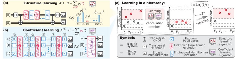
Figure 1: (a) Quantum circuit for the structure-learning subroutine $\mathcal{A}^{I}$. It prepares n pairs of 2-qubit Bell states between the original and ancillary systems via transversal gates. The original system then evolves coherently under the unknown Hamiltonian $H$ and the engineered Hamiltonian $H_{*}$, where $H_{*}$ consists of the large terms in $H$ learned in previous steps with an opposite sign. The combined system is then measured on the n-pair Bell basis. Nontrivial outcomes have probabilities proportional to $\mu_{i}^{2}$, enabling inference of the interaction structure. (b) Quantum circuit for the coefficient-learning subroutine $\mathcal{A}^{II}$. By inserting random Pauli gates from a designed set into the unknown Hamiltonian’s evolution, the time evolution of a specific term is approximated, allowing the interaction strength $\mu_{s}$ to be extracted via robust frequency estimation. (c) Combining these subroutines enables hierarchical coefficient estimation, achieving Heisenberg-limited scaling.

In this work, we propose a novel Hamiltonian learning algorithm that overcomes these limitations. Our method achieves Heisenberg-limited scaling for arbitrary Hamiltonians, including non-local ones, with the total experimental time scaling polynomially with the number of Pauli terms in the Hamiltonian. To be more explicit, any $n$-qubit Hamiltonian $H$ can be expressed in the form:

$$H=\sum_{s\in\mathcal{S}}\mu_{s}P_{s},$$ (1)

with $P_{s}$ the $n$-qubit traceless Pauli operators, $\mathcal{S}$ the set of Pauli operators from which $H$ is constituted, and $|\mu_{s}|\leq 1$ the unknown coefficients. Furthermore, we use $M$ to denote the number of Pauli terms with nonzero coefficients in $H$.

Without prior knowledge of which terms are in the Hamiltonian and what the coefficient values are, there are two specific difficulties for learning such a Hamiltonian: 1. what is the structure $\mathcal{S}$, the $M$ Pauli terms, of this Hamiltonian; 2. what are the coefficients $\mu_{s}$ with respect to each term in this Hamiltonian. We tackle these difficulties by cycling through an alternating hierarchy of two steps: structure learning and coefficient learning. In the structure learning phase, we identify the Pauli terms with large coefficients by direct sampling a simple quantum circuit, where terms with large coefficients will dominate the outcome. In the coefficient learning phase, we isolate the identified terms by applying ensembles of single-qubit Pauli gates, similar to techniques such as dynamical decoupling [33, 34, 35, 36] or Hamiltonian reshaping [11, 12]. We then estimate the coefficients through robust frequency estimation [37]. Our algorithm not only achieves Heisenberg-limited scaling in terms of total experimental time but is also resilient to state-preparation-and-measurement (SPAM) errors.

To the best of our knowledge, this is the first quantum algorithm capable of learning arbitrary Hamiltonians with Heisenberg-limited scaling using only product state inputs, single-qubit measurements, and black-box access to the Hamiltonian dynamics. This work not only resolves a long-standing theoretical question about Hamiltonian learning but also introduces a practical algorithm with minimal experimental requirements.

II The learning protocol

We consider learning an unknown many-body Hamiltonian $H$ as expressed in Equation 1 through time evolution $e^{-iHt}$ with arbitrary $t$ and a programmable quantum computer. Here we provide a more detailed explanation of how our protocols cycle through an alternating hierarchy of structure learning and coefficient learning steps. In the structure-learning step, we identify the dominant interaction terms by determining the support of the coefficient vector $\bm{\mu}=(\mu_{1},\mu_{2},\ldots,\mu_{4^{n}-1})^{T}$. To achieve this, we introduce two approaches: one (denoted as $\mathcal{A}^{I}$) employs $n$ pairs of 2-qubit Bell states shared between the original system and an ancillary system of the same size, while the other (denoted as $\mathcal{A}^{I^{\prime}}$) uses only product state inputs and single-qubit measurements, eliminating the need for ancillary systems at the cost of a moderate increase in $M$-dependence. In the coefficient learning (denoted as $\mathcal{A}^{II}$) step, we estimate the coefficients of Pauli operators identified in the preceding structure-learning phase. Specifically, we first determine all the Pauli operators with coefficients $1/2<|\mu_{i}|\leq 1$, and learn their coefficients $\mu_{i}$. We then repeat those two steps for smaller coefficient ranges $1/4<|\mu_{i}|\leq 1/2$ and so on. In the $k$-th iteration, we learn coefficients that are $(1/2)^{k}<|\mu_{s}|\leq(1/2)^{k-1}$, continuing until $k=\lceil\log_{2}(1/\epsilon)\rceil$, where $\epsilon$ is the desired learning precision. This hierarchical learning strategy achieves the gold standard Heisenberg-limited scaling, requiring a total experimental time having $1/\epsilon$ dependence up to a polylogarithmic factor to reach $\epsilon$-learning accuracy.

In the follows, we use $\widetilde{\mathcal{O}}(f)$ to omit $\text{polylog}(f)$ scaling factors. The main results of the hierarchical learning algorithm are summarized as follows:

Result 1 (Informal version of Theorem 1).

There exists a quantum algorithm for learning the unknown Hamiltonian $H$ as in Equation 1 taking $n$ pairs of $2$-qubit Bell state as input for each experiment instance, querying to real-time evolution of $H$, and performing Bell-basis measurements that outputs estimation $\hat{\bm{\mu}}$ such that

$$||\hat{\bm{\mu}}-\bm{\mu}||_{\infty}\leq\epsilon$$ (2)

with high probability. The total experimental time is

$$T=\widetilde{\mathcal{O}}\left(M^{2}/\epsilon\right).$$ (3)

This algorithm has trivial classical post-processing and is robust against SPAM errors.

Result 2 (Informal version of Theorem 2).

There exists an ancilla-free algorithm quantum algorithm for learning the unknown Hamiltonian $H$ as in Equation 1 with product-state input, queries to real-time evolution of the Hamiltonian, and single-qubit measurements that outputs $\hat{\bm{\mu}}$ achieving (2) with high probability. The total experimental time $T$ is

$$T^{\prime}=\widetilde{\mathcal{O}}\left(M^{3}\log(n)/\epsilon\right).$$ (4)

This algorithm needs classical post-processing with time

$$T^{C}=\widetilde{\mathcal{O}}(M^{5}n\log(n))$$ (5)

and is robust against SPAM errors.

In the following, we will outline the proof for both results by introducing the algorithms on structure learning ($\mathcal{A}^{I}$ and $\mathcal{A}^{I^{\prime}}$) and coefficients learning ($\mathcal{A}^{II}$), and the corresponding proof ideas.

II.1 Structure-learning algorithm

We first consider the structure-learning algorithm $\mathcal{A}^{I}$ taking $n$ pairs of Bell states between the original system and a $n$-qubit ancillary system as input. To start, consider a simple task: suppose all the unknown coefficients in the Hamiltonian are not small, i.e. $\mu_{m}:=\min\mu_{s}=\mathcal{O}(1)$. One of the challenges in identifying the support $\mathcal{S}$ originates from the fact that the Pauli operators in the Hamiltonian do not necessarily commute with each other. To mitigate this difficulty, we combine the Bell sampling circuit with the coherent evolution driven by $H=\sum_{s}\mu_{s}P_{s}$ for time $\tau$. We prepare $n$ pairs of $2$-qubit Bell states $\ket{\Phi^{+}}^{\otimes n}=\left(\frac{\ket{00}+\ket{11}}{\sqrt{2}}\right)^{\otimes n}$ with transversal Hadamard and CNOT gates. The first $n$ qubit undergoes the short-time evolution of $H$ with the second $n$ qubits idle. We then perform a Bell-basis measurement with transversal Hadamard and CNOT gates. The quantum circuit is visualized in Fig. 1 (a). This quantum circuit effectively achieves direct sampling from the probability distribution $p(s|\bm{\mu})$ related to the support of $\bm{\mu}$. To see this, we take a single-qubit Hamiltonian $H=\mu_{x}X+\mu_{y}Y+\mu_{z}Z$ as the instance for illustration. The first qubit of the Bell state undergoes the short-time evolution of $H$ and the evolved state becomes

$$\begin{split}&\ket{\Phi^{+}}-i\tau(\mu_{x}XI+\mu_{y}YI+\mu_{z}ZI)\ket{\Phi^{+}}+\mathcal{O}(\tau^{2})\\ &=\ket{\Phi^{+}}-i\tau\mu_{x}\ket{\Psi^{+}}-i\tau\mu_{y}\ket{\Psi^{-}}-i\tau\mu_{z}\ket{\Phi^{-}}+\mathcal{O}(\tau^{2}),\end{split}$$ (6)

where $\ket{\Phi^{\pm}}$ and $\ket{\Psi^{\pm}}$ are the four Bell basis states. Therefore, the outcome probability of each Bell basis state is proportional to $\mu_{i}^{2}\tau^{2}$. This can be generalized to multi-qubit systems. If one sets $\tau=\mathcal{O}(\mu_{m}/M)$, we show the outcome distribution can be lower-bounded as $p(s|\bm{\mu})>\Omega\left(\mu_{m}^{4}/M^{2}\right)$ (see Section C.5 for details). Therefore, with the union bound, one can sample all support $\mathcal{S}=\{s:|\mu_{s}|\geq\mu_{m}\}$ at least once with high probability by querying this quantum circuit $\mathcal{O}(\log(M)/\mu_{m}^{2}\tau^{2})$ times. The total evolution time under $H$ is $\mathcal{O}(M\log(M)/\mu_{m}^{3})$.

Due to the finite-time evolution, different terms in $\mathcal{S}$ get multiplied together in second and higher orders as a result of Taylor expansion. If there is an $s$ with vanishing $\mu_{s}$ triggering a false-positive detection, one can always discard it in the coefficient learning step after realizing $\mu_{s}$ is smaller than the desired threshold $\mu_{m}$. Note that the worst case number of false-positive events is also upper bounded by the number of samples $\mathcal{O}(M^{2}\log(M))$.

It is natural to ask whether the entanglement in the structure learning step is necessary. Surprisingly, we provide a negative answer to this question by showing an alternative algorithm with product state input and single-qubit measurement at the cost of a moderate increase in $M$ dependence. The key observation is that applying random Pauli gates before and after the evolution $e^{-iH\tau}$ will transform it into an effective Pauli channel, a process called Pauli twirling [38, 39, 40, 41, 42]. In the single-qubit instance, the effective channel after applying random Pauli gates is

$$\begin{split}\Lambda_{P}(\rho)&=\underset{\sigma_{T}\sim\mathbb{P}}{\mathbb{E}}\sigma_{T}^{\dagger}e^{-iH\tau}\sigma_{T}\rho\sigma_{T}^{\dagger}e^{iH\tau}\sigma_{T}\\ &\approx\rho+\mu_{x}^{2}\tau^{2}X\rho X+\mu_{y}^{2}\tau^{2}Y\rho Y+\mu_{z}^{2}\tau^{2}Z\rho Z,\end{split}$$ (7)

which is a Pauli channel with Pauli error rates $\mu_{i}^{2}\tau^{2}$. It can be generalized to multi-qubit systems by applying random Pauli gates on each qubit. Employing the Pauli error rates estimation protocol using product state inputs and single-qubit measurements [43], we obtain an alternative approach $\mathcal{A}^{I^{\prime}}$ for structure learning. In Appendix F, we provide the details of this approach.

II.2 Coefficient-learning algorithm

The coefficient-learning algorithm $\mathcal{A}^{II}$ takes the structure $\mathcal{S}$ as input and outputs the coefficients $\{\mu_{s}:s\in\mathcal{S}\}$. The key idea is to isolate each term $\mu_{s}P_{s}$ during the evolution and learn each individual coefficient $\mu_{s}$. The first step can be achieved by Hamiltonian reshaping [11, 12], which inserts random single-qubit Pauli gates between evolutions of $H$. Each $\mu_{s}$ can be learned with Heisenberg-limited scaling using robust frequency estimation [37, 12].

II.2.1 Hamiltonian reshaping

The goal of Hamiltonian reshaping is to approximate the time evolution of a specific term or a subset of commuting Pauli terms in $H$. We focus on the case where the target Hamiltonian after reshaping is a single traceless Pauli operator $P_{s}$ for illustration. Define $\mathcal{K}_{P_{s}}$ as the set containing all Pauli operators that commute with $P_{s}$. For any traceless Pauli operator $P_{l}\neq P_{s}$, the ensemble average of the transformed operator $P^{\dagger}P_{l}P$ over set $\mathcal{K}_{P_{s}}$ will result in zero, since half of the Pauli operators in $\mathcal{K}_{P_{s}}$ commute with $P_{l}$ and the other half anti-commute with it. On the other hand, for $P_{s}$, since every Pauli operator in $\mathcal{K}_{P_{s}}$ commutes with it, this transformation will leave $P_{s}$ unchanged.

In the Hamiltonian learning scenario, we want to learn the coefficients of each Pauli term $P_{s}$ given by the previous structure learning step one at a time. For a given $P_{s}$, we insert a randomly sampled Pauli operator from $\mathcal{K}_{P_{s}}$ between the short-time evolutions under $H$. By concatenating randomly transformed short-time unitary evolutions, we realize a quantum channel similar to the randomized Hamiltonian simulation algorithm, such as qDRIFT [44, 45]. We then show this channel will be at most $\mathcal{O}(M^{2}t^{2}/r_{2})$ far from the desired evolution $e^{-i\mu_{s}P_{s}t}$ in the diamond distance, where $r_{2}$ is the number of short-time evolution steps (see Section D.1 for details).

II.2.2 Robust frequency estimation

With a good approximation of the time evolution channel under a single-term Hamiltonian $H_{\mathrm{eff}}=\mu_{s}P_{s}$ by Hamiltonian reshaping, we can robustly estimate $\mu_{s}$ to an accuracy $\epsilon$ with Heisenberg-limited scaling using the robust frequency estimation protocol. This protocol follows the same idea as the robust phase estimation protocol [37], but is modified to use only product-state input and to a good confidence interval rather than minimizing the mean-squared error.

Consider a simple example with $P_{s}=IZZX$ and unknown $\mu_{s}$. We design the following two experiments: 1. the ($+$) experiment with input state $|\psi_{+}\rangle=\ket{0}\otimes\ket{+}\otimes\ket{0}\otimes\ket{+}$ and measuring observable $O_{+}=IXZX$ after evolution time $t$; 2. the ($-$) experiment with input state $|\psi_{-}\rangle=\ket{0}\otimes\ket{-}\otimes\ket{0}\otimes\ket{+}$ and measuring observable $O_{-}=IYZX$ after evolution time $t$. It can be easily verified that the expectation values are $\langle O_{+}\rangle=\cos(2\mu_{s}t)$ and $\langle O_{-}\rangle=\sin(2\mu_{s}t)$, which together form a simple oscillation $e^{i2\mu_{s}t}$. The idea of robust frequency estimation is to narrow down the frequency $\theta$ of an oscillation signal $e^{i\theta t}$ in a hierarchical manner. Given $\theta\in[a,b]$, one can correctly distinguish whether $\theta$ is in $\theta\in[a,(a+2b)/3]$ or in $\theta\in[(2a+b)/3,b]$ by finite sampling in $t=\pi/(b-a)$. This process is then repeated $\mathcal{O}\left(\log_{3/2}((b-a)/\epsilon)\right)$ times with the range divided by $2/3$ each time. The choice of the overlapped region makes this method robust against errors. In Section D.2, we describe the setup of the robust frequency estimation for arbitrary Pauli operator and show it is robust against finite-sample error and channel approximation error from the Hamiltonian reshaping.

II.3 Hierarchical learning and scaling analysis

As we have described above, $\mathcal{A}^{I}$ (or $\mathcal{A}^{I^{\prime}}$) can learn the structure of the Hamiltonian and $\mathcal{A}^{II}$ can estimate the coefficients. However, directly concatenating $\mathcal{A}^{I}$ (or $\mathcal{A}^{I^{\prime}}$) with $\mathcal{A}^{II}$ will give an algorithm with a complexity of $\widetilde{\mathcal{O}}(1/\epsilon^{3})$ dependence on the target accuracy $\epsilon$, not enough for achieving Heisenberg-limited scaling. We address this issue by introducing a hierarchical learning protocol, where we divide the terms in $H$ into $J=\left\lceil\log_{2}(1/\epsilon)\right\rceil$ levels. For the $j$-th level, we learn all terms with coefficient $2^{-(j+1)}<|\mu_{s}|\leq 2^{-j}$ to $\epsilon$ accuracy by applying $\mathcal{A}^{I}$ (or $\mathcal{A}^{I^{\prime}}$) and $\mathcal{A}^{II}$. Moreover, since we already have an estimation of coefficients for terms with $2^{-j}\leq\mu_{s}$, we can approximately cancel out those terms by interfacing the black-box evolution with the quantum computer in Hamiltonian simulation. We then rescale the Hamiltonian by extending the evolution time, thereby boosting the initially small coefficients in $j$-th level to a constant scale. The steps of this procedure are depicted in Figure 1 (c). Both the term cancellation and rescaling can be achieved using Trotterization (see Appendix C for details).

We now analyze the scaling of total experimental time. We first consider the structure learning algorithm $\mathcal{A}^{I}$. For each sample $l$ and each $j\in\{0,1,\ldots,\left\lceil\log_{2}(1/\epsilon)\right\rceil-1\}$, the total evolution time is $t^{(1)}_{j,l}=\mathcal{O}(2^{j}/M)$ where $2^{j}$ comes from the rescaling of the Hamiltonian. As shown before, we need $L=\widetilde{\mathcal{O}}(M^{2})$ samples to learn the structure in $j-$th level. The total evolution time for $\mathcal{A}^{I}$ is

$$\begin{split}T_{1}=\sum_{j=0}^{\lceil\log_{2}(1/\epsilon)\rceil-1}\sum_{l=1}^{L}t^{(1)}_{j,l}=\widetilde{\mathcal{O}}(M/\epsilon).\end{split}$$ (8)

For Hamiltonian coefficients learning algorithm $\mathcal{A}^{II}_{j}$, the total evolution time for learning each coefficient to $\epsilon$ accuracy with robust frequency estimation scales as $t^{(2)}_{j,l}=\widetilde{\mathcal{O}}\left(1/\epsilon\right)$. There could be false-positive detections in the structure learning. In the worst cases, we need to estimate the frequencies up to $L_{j}=\widetilde{\mathcal{O}}(M^{2})$ terms. Thus the total evolution time of the Hamiltonian coefficient algorithm $\mathcal{A}^{II}$ is

$$\begin{split}T_{2}&=\sum_{j=0}^{\lceil\log_{2}(1/\epsilon)\rceil-1}L_{j}t^{(2)}_{j,l}=\widetilde{\mathcal{O}}(M^{2}/\epsilon).\end{split}$$ (9)

In addition, we show this protocol is robust against SPAM errors (see Appendix C) and the time complexity with the alternative approach is provided in Appendix F.

III Trade-off between total evolution time and quantum control

Compared to previous approaches for learning Hamiltonians through their eigenstates or Gibbs states, our protocols exceed the standard quantum limit and achieve Heisenberg-limited scaling. This is accomplished by sequentially querying the real-time evolutions of the Hamiltonian, interleaved with discrete quantum controls. A natural question is whether quantum controls are necessary for achieving Heisenberg-limited scaling. We answer this question affirmatively by proving a trade-off between the total evolution time complexity for an unknown Hamiltonian $H$ and the number of discrete quantum controls.

Intuitively, we can generalize experiments with discrete quantum controls and sequential queries to the Hamiltonian as the following theoretical model. Given a Hamiltonian $H$ with coefficient vector $\bm{\mu}$ defined in (1), the protocol performs multiple experiments and measures at the end of each experiment. In each experiment, the protocol prepares an input state (possibly with ancilla qubits) and queries the Hamiltonian multiple times with a discrete quantum control channel between every two neighboring queries. The protocol can be adaptive in the sense that it can dynamically decide how to prepare the input state, query the real-time evolutions, perform quantum controls, and measure the final state based on the history of the previous experiments. We provide the formal definition of this model in Appendix G. In a recent work [46], it is shown through quantum Fisher information [47, 48, 49] that for unbiased learning algorithm, Heisenberg-limited scaling is not possible in the absence of quantum control. Here, we prove a lower bound in a rigorous and most general fashion for any possible adaptive and biased protocols that might have access to ancillary quantum memory.

Result 3 (Informal version of Theorem 12).

Any protocol, which is possibly adaptive, biased, and ancilla-assisted, with total evolution time $T$ and at most $\mathcal{L}$ discrete quantum controls per experiment requires $T=\Omega(\mathcal{L}^{-1}\epsilon^{-2})$ to estimate the coefficient of the unknown Hamiltonian $H$ within additive error $\epsilon$.

Note that this result indicates that, in general, it is impossible for any protocol to achieve Heisenberg-limited scaling without at least $\mathcal{L}=\Omega(1/\epsilon)$ discrete quantum controls per experiment. On the other hand, this trade-off does not suggest the existence of Hamiltonian learning algorithms that can surpass the Heisenberg limit provided a sufficient number of discrete quantum controls. In fact, as proved in [11, 12, 46], there is a strict $T=\Omega(1/\epsilon)$ lower bound for the total evolution time. The high-level strategy of our proof is to combine the learning tree framework [50] equipped with the martingale trick [51, 52, 53] and quantum Fisher information. We model any learning protocol as a decision tree, and any choice of unknown Hamiltonian $H$ corresponds to a distribution on the leaves. We then find a pair of Hamiltonians $H$ and $H^{\prime}$ such that induced probability distributions on the leaves are statistically indistinguishable unless the $T$ and $\mathcal{L}$ are large enough. Details of the proof are in Appendix G.

IV Outlook

In this work, we propose the first ansatz-free Hamiltonian learning protocol for a $n-$qubit system without imposing any interaction structural assumptions. The total experimental time is polynomial in the number of interactions, and also achieves the gold standard $\mathcal{O}(1/\epsilon)$ Heisenberg scaling. Notably, our protocol relies solely on queries to the black-box time evolution of the unknown Hamiltonian with elementary digital controls of a quantum computer. Furthermore, we establish a fundamental trade-off between total evolution time and quantum control in Hamiltonian learning algorithms in the most general setting.

This work opens up new avenues for Hamiltonian learning in future research. On the theoretical side, our protocol requires coherent evolution of the unknown Hamiltonian for $\mathcal{O}(1/\epsilon)$ total time to achieve an estimation error $\epsilon$. In practice, however, the system may experience noise, which could introduce an error floor—beyond which Heisenberg-limited scaling may still persist. Understanding how noise affects the scaling and exploring whether error correction or mitigation can restore Heisenberg-limited performance remain open questions. In particular, techniques from quantum metrology may offer valuable insights in this direction [54, 55].

V Acknowledgements

We are thankful for the insightful discussions with Sitan Chen, Friedrich Liyuan Chen, Soonwon Choi, Dong-Ling Deng, Nik O. Gjonbalaj, Yingfei Gu, Hsin-Yuan Huang, Christian Kokail, Yunchao Liu, Francisco Machado, Daniel K. Mark, and Pengfei Zhang.

CONTENTS

A.  NOTATIONSA

B.  MAIN RESULTS AND PROOF IDEASB

C.  HAMILTONIAN STRUCTURE LEARNING $\mathcal{A}^{I}_{j}$ C

1. Hamiltonian simulation with TrotterizationC.1
2. Taylor expansion of the time evolution operatorC.2
3. Bell samplingC.3
4. SPAM errorC.4
5. Lower bound for the probability of elements in $\mathfrak{S}_{j}$C.5
6. Determine the high-probability elements of a sparse probability distributionC.6
7. The complexity of $\mathcal{A}_{j}^{I}$C.7

D.  HAMILTONIAN COEFFICIENT LEARNING $\mathcal{A}^{II}_{j}$ D

1. Hamiltonian reshapingD.1
2. Robust frequency estimationD.2
3. The experimental setup of $\mathcal{A}_{j}^{II}$D.3
4. The complexity of $\mathcal{A}_{j}^{II}$D.4

E.  TOTAL EVOLUTION TIME COMPLEXITY E

F.  ALTERNATIVE SINGLE-COPY PRODUCT STATE INPUT APPROACH $\mathcal{A}^{I^{\prime}}_{j}$ F

1. Pauli error rate for time-evolution channelF.1
2. Estimating Pauli error rates via population recoveryF.2
3. Complexity of $\mathcal{A}^{I^{\prime}}_{j}$F.3
4. Totoal evolution time complexity of the single-copy product state input Hamiltonian learning protocolF.4

G.  THE PROOF FOR THE TRADE-OFF G

Appendix A Notations

In this work, the Pauli matrices are denoted by $\sigma^{x},\sigma^{y},\sigma^{z}$. We use the following notation to denote the Pauli eigenstates:

$$\ket{1,z}=\ket{0},\quad\ket{-1,z}=\ket{1},\quad\ket{1,x}=\ket{+},\quad\ket{-1,x}=\ket{-},$$ (10)

$$\ket{1,y}=\frac{1}{\sqrt{2}}(\ket{0}+i\ket{1}),\quad\ket{-1,y}=\frac{1}{\sqrt{2}}(\ket{0}-i\ket{1}).$$

We denote the set of all $N$-fold tensor products of single-qubit Pauli matrices (and the identity) by $\mathbb{P}_{n}$:

$$\mathbb{P}_{n}=\left\{\bigotimes_{i=1}^{n}P_{i}:P_{i}=I,\sigma^{x},\sigma^{y},\text{ or }\sigma^{z}\right\}.$$ (11)

We use the following notation for the four maximally entangled 2-qubit states

$$\begin{split}&\ket{\Phi^{+}}=\dfrac{\ket{00}+\ket{11}}{\sqrt{2}}\\ &\ket{\Phi^{-}}=\dfrac{\ket{00}-\ket{11}}{\sqrt{2}}\\ &\ket{\Psi^{+}}=\dfrac{\ket{10}+\ket{01}}{\sqrt{2}}\\ &\ket{\Psi^{-}}=i\dfrac{\ket{10}-\ket{01}}{\sqrt{2}},\end{split}$$ (12)

which are also the four eigenstates of the Bell-basis measurement. In the following, we will also use $\ket{\mathrm{EPR}_{n}}=\ket{\Phi^{+}}^{\otimes n}$.

We consider the $N$-qubit traceless Hamiltonian to be learned as

$$H=\sum_{s}\mu_{s}P_{s},\quad|\mu_{s}|\leq 1,$$ (13)

where $P_{s}\in\mathbb{P}_{N}\setminus\{I^{\otimes N}\}$. Let $M$ be the number of terms in the coefficient vector $\bm{\mu}=(\mu_{1},\mu_{2},\ldots,\mu_{4^{N}-1})^{T}$ which are larger than the threshold constant $\epsilon\in(0,1)$; this is the sparsity of $H$.

Let $S\subseteq\mathbb{P}_{n}$ be the set of the indices $s$ of terms $P_{s}$ in $H$ with coefficients $|\mu_{s}|>\epsilon$. For $j\in\{0,1,2,\ldots,\left\lceil\log_{2}(1/\epsilon)\right\rceil\}$, define the set $S_{j}$ of all indices $s$ of terms $P_{s}$ in $H$ such that their coefficients $\mu_{s}$ satisfy $|\mu_{s}|\leq 2^{-j}$:

$$S_{j}=\{s:s\in S,|\mu_{s}|\leq 2^{-j}\},\quad j\in\{0,1,2,\ldots,\left\lceil\log_{2}(1/\epsilon)\right\rceil\},$$ (14)

note that $S=S_{0}$. Let the set $\mathfrak{S}_{j}=S_{j}\setminus S_{j+1}$ be the set of all indices $s$ of terms $P_{s}$ in $H$ such that their coefficients $\mu_{s}$ satisfy $2^{-(j+1)}<|\mu_{s}|\leq 2^{-j}$:

$$\mathfrak{S}_{j}=\{s:s\in S,2^{-(j+1)}<|\mu_{s}|\leq 2^{-j}\},\quad j\in\{0,1,2,\ldots,\left\lceil\log_{2}(1/\epsilon)\right\rceil-1\}.$$ (15)

Let $U_{H}(t)=e^{-iHt}$ to represent the time evolution operator under $H$. Let $\ket{\mathrm{EPR}}=\frac{1}{\sqrt{2}}(\ket{00}+\ket{11})$ be the $2$-qubit EPR state, and let $\ket{\mathrm{EPR}_{n}}=\bigotimes_{j=1}^{n}\ket{\mathrm{EPR}}$ be the $2n$-qubit EPR state.

Consider a general quantum channel $\Lambda$. One can write it in its Kraus operator expression as

$$\Lambda(\rho)=\sum_{k}K_{k}\rho K_{k}^{\dagger},$$ (16)

where $\sum_{k}K_{k}^{\dagger}K_{k}=I$.

Expanding the Kraus operator in the Pauli basis, we find

$$K_{j}=\sum_{\sigma_{k}\in\{I,\sigma_{x},\sigma_{y},\sigma_{z}\}}\alpha_{j,k}\sigma_{k}.$$ (17)

Appendix B Main results and proof ideas

The main result of Hamiltonian learning with ancillary systems can be summarized as

Theorem 1 (2-copy Heisenberg-limited Hamiltonian learning algorithm).

For an arbitrary $n$-qubit unknown Hamiltonian $H=\sum_{s\in S}\mu_{s}P_{s}$, with $|\mu_{s}|\leq 1$ and $|S|\leq M$, there exists a hierarchical learning quantum algorithm which only queries the black box forward evolution of $H$, and a fault-tolerant quantum computer with $n$ ancillary qubits that outputs a classical description $\hat{\mu}_{s}$ of $\mu_{s}$ such that $|\hat{\mu}_{s}-\mu_{s}|<\epsilon$ with probability at least $1-\delta$, and the total experimental time is

$$T=\mathcal{O}\left(\frac{M^{2}\log(M/\delta)[\log(1/\epsilon)]^{2}}{\epsilon}\right).$$

This algorithm requires no non-trivial classical post-processing and is robust against SPAM error.

In addition, we proposed a single-copy Hamiltonian learning algorithm without an ancillary system using only single-qubit operations, which can be summarized as:

Theorem 2 (Single-copy Heisenberg-limited Hamiltonian learning algorithm).

For an arbitrary $n$-qubit unknown Hamiltonian $H=\sum_{s\in S}\mu_{s}P_{s}$, with $|\mu_{s}|\leq 1$ and $|S|\leq M$, there exists a hierarchical learning quantum algorithm which only queries the black box forward evolution of $H$, and a fault-tolerant quantum computer with no ancillary qubits that outputs a classical description $\hat{\mu}_{s}$ of $\mu_{s}$ such that $|\hat{\mu}_{s}-\mu_{s}|<\epsilon$ with probability at least $1-\delta$, and the total experimental time is

$$T=\mathcal{O}\left(\frac{M^{3}(\log(Mn)\log(1/\epsilon)+\log(M/\delta)[\log(1/\epsilon)]^{2})}{\epsilon}\right).$$

This algorithm requires a total classical post-processing time

$$T^{C}=\mathcal{O}\left(M^{5}n\log(Mn/\delta)\log(1/\epsilon)\right)$$

The main subroutine of our learning algorithms is defined as follows:

Definition 1 (Hierarchical learning subroutine).

Given 1. an unknown Hamiltonian $H=\sum_{s\in S}\mu_{s}P_{s}$, with $|\mu_{s}|\leq 1$ and $|S|\leq M$, and 2.the classical description of $\hat{H}_{j}$ (its Pauli operator terms and coefficients), an estimation of all coefficients larger than $2^{-j}$ up to $\epsilon$ term-wise error. There exists a hierarchical learning subroutine $\mathcal{A}_{j}$ to obtain $\hat{H}_{j+1}$ which is an estimation of all coefficients larger than $2^{-(j+1)}$ up to $\epsilon$ term-wise error, for $j=0,1,2,\ldots,\lceil\log_{2}(1/\epsilon)\rceil-1$. The final estimation $\hat{H}_{\lceil\log_{2}(1/\epsilon)\rceil-1}$ will be a characterization of $H$ to $\epsilon$ term-wise error.

The main ideas: Based on the definitions provided in the previous section, we partition all unknown coefficients into the following sets: $S=\mathfrak{S}_{0}\cup\mathfrak{S}_{1}\cup\dots\cup\mathfrak{S}_{\lceil\log_{2}(1/\epsilon)\rceil-1}$, where $\mathfrak{S}_{j}=\{s:s\in S,2^{-(j+1)}<|\mu_{s}|\leq 2^{-j}\}$. At each step $j$, the hierarchical learning subroutine $\mathcal{A}_{j}$ first identifies the index $s\in\mathfrak{S}_{j}$ with high probability using the Hamiltonian structure learning algorithm $\mathcal{A}_{j}^{I}$. With this information, the corresponding coefficients can then be learned using the Hamiltonian coefficient learning algorithm $\mathcal{A}_{j}^{II}$. Below, we provide an overview of the key components of both algorithms, with a detailed analysis deferred to the subsequent sections.

In the Hamiltonian structure learning $\mathcal{A}_{j}^{I}$, we first create the EPR state between unknown system with $N$-qubit ancillary system using transversal gates. Then we perform the time evolution of the unknown system under $\tilde{H}_{j}=(H-\hat{H}_{j})/2^{-j}$ for time $t$ by querying unknown system and a fault-tolerant quantum computer iteratively. Lastly, we perform the Bell-basis measurement on the $2N$-qubit system. We prove that if $t=\mathcal{O}\left(\frac{1}{CM}\right)$ where $C$ is a big constant to supress the error, then all elements $s=\mathfrak{S}_{j}$ will be sampled once with high probability. There are several approximation errors involved in this step: 1. Trotterization error ($\varepsilon_{\mathrm{Trotter}}$) for simulating time-evolution under $\tilde{H}_{j}$, 2. truncation error ($\varepsilon_{\mathrm{Taylor}}$) from the Taylor expansion of time $t=\mathcal{O}\left(\frac{1}{CM}\right)$ evolution, and SPAM errors ($\varepsilon_{\mathrm{SPAM}}$). In Lemma 3, we prove that for elements in $\mathfrak{S}_{j}$, their probability is lower bounded by $\widetilde{\Omega}\left(\frac{1}{4C^{2}M^{2}}-\frac{1}{C^{3}M^{2}}-\frac{2^{2j}}{C^{2}r}-\varepsilon_{\text{SPAM}}\right)$, where $r$ is the Trotter steps. Then one can sample all elements in $\mathfrak{S}_{j}$ at least once with probability $1-\delta$ by querying this algorithm $\mathcal{O}(C^{2}M^{2}\log(M/\delta))$ times. Then the total evolution time of all $\mathcal{A}^{I}_{j}$ is $\mathcal{O}\left(\frac{M\log(M/\delta)}{\epsilon}\right)$, which reaches the Heisenberg-limited scaling.

Then we use the Hamiltonian coefficient learning $\mathcal{A}^{II}_{j}$ to learn the coefficients $\mu_{s}$ for $s$ in the set $\widetilde{\mathfrak{S}_{j}}$, which we identified in the previous step. There are at most $|\widetilde{\mathfrak{S}_{j}}|\equiv L_{j}=\mathcal{O}(M^{2}\log(M/\delta))$ terms sampled in the previous step. We first use the Hamiltonian reshaping technique as introduced in Section D.1 to approximate the time-evolution under a single term $P_{s}$ for $s\in\widetilde{\mathfrak{S}_{j}}$. We show the approximation error is bounded by $\mathcal{O}(\frac{M^{2}t^{2}}{r_{2}})$ for total evolution time $t$ with $r_{2}$ Trotter steps. Then we adapt the robust frequency estimation (RFE) as introduced in Section D.2 to estimate $\mu_{s}$ within $\epsilon$ accuracy. In Theorem 7, we show the total evolution time in each RFE procedure is $\mathcal{O}(\frac{\log(1/\epsilon)+\log\log(2^{-j}/\epsilon)}{\epsilon})$. As there are at most $L_{j}$ terms, the total evolution time for $\mathcal{A}_{j}^{II}$ is $\mathcal{O}(\frac{M^{2}\log(M/\delta)(\log(1/\epsilon)+\log\log(2^{-j}/\epsilon))}{\epsilon})$, which also reaches the Heisenberg-limited scaling. Moreover, since we estimate each coefficient at a time, the effective Hamiltonian $H_{eff}$ after reshaping is a single term Hamiltonian, we only need product state input in RFE instead of highly entangled Bell state input as in [12].

In Section F, we investigate whether quantum entanglement of the 2-copy in structure learning is necessary. Surprisingly, we found a novel structure learning algorithm that only uses product state input without any ancillary qubits that also achieves the Heisenberg limit when used in the Hierarchical learning subroutine.

In Section G, we provide rigorous proofs for the lower bound of the general Hamiltonian learning algorithm in Theorem 12, where we utilized the learning tree representation and applied Le Cam’s two-point method for Hamiltonian distinguishing problem. The lower bound implies that for a Hamiltonian learning algorithm, there is a trade-off between the total evolution time complexity and the number of quantum controls.

Appendix C Hamiltonian structure learning $\mathcal{A}^{I}_{j}$

We here provide details for Hamiltonian structure learning $\mathcal{A}^{I}_{j}$. In $\mathcal{A}^{I}_{j}$, we first use Trotterization to approximate the time evolution channel under $\tilde{H}_{j}=(H-\hat{H}_{j})/2^{-j}$. Then, we evolve an $N$-qubit EPR state into this channel and perform a Bell-basis measurement at the end. By analyzing the Taylor expansion of the time evolution operator, and analyzing how considering the probability distribution of Bell-basis measurement will deviate if only considering the first-order truncation. Taking the Trotterization error $\varepsilon_{\text{Trotter}}$, first-order truncation error $\varepsilon_{\text{Taylor}}$, error caused by the imperfections of $\hat{H}_{j}$, and the state-preparation and measurement (SPAM) error $\varepsilon_{\text{SPAM}}$ into consideration, we show that $\mathcal{A}^{I}_{j}$ can identify all the terms in $H$ that is larger than $2^{-(j+1)}$ with high probability.

C.1 Hamiltonian simulation with Trotterization

By the Lie product formula, the time evolution operator $e^{-i\tilde{H}_{j}t}$ can be approximated by interleaving the time evolution operator $e^{-iHt/(2^{-j}r)}$ and $e^{i\hat{H}_{j}t/(2^{-j}r)}$ in the asymptotic limit

$$e^{-i\tilde{H}_{j}t}=e^{-i(H-\hat{H}_{j})t/2^{-j}}=\lim_{r\rightarrow\infty}\left(e^{-iHt/(2^{-j}r)}e^{i\hat{H}_{j}t/(2^{-j}r)}\right)^{r},$$ (18)

where $e^{i\hat{H}_{j}t/(2^{-j}r)}$ is realizable through Hamiltonian simulation since the classical characterization of $\hat{H}_{j}$ is known.

We consider $r$ is a finite integer, then by the Trotter-Suzuki formula [56, 57, 58, 59], we have

$$e^{-i\tilde{H}_{j}t}=e^{-i(H-\hat{H}_{j})t/2^{-j}}=\left(e^{-iHt/(2^{-j}r)}e^{i\hat{H}_{j}t/(2^{-j}r)}\right)^{r}+\mathcal{O}\left([H,\hat{H}_{j}]\frac{(t/2^{-j})^{2}}{r}\right).$$ (19)

To characterize the accuracy of approximating the time evolution channel, denote the time evolution channel under the Hamiltonian $\tilde{H}_{j}$ as

$$\mathcal{U}_{\tilde{H}_{j},t}(\rho)=e^{-i\tilde{H}_{j}t}\rho e^{i\tilde{H}_{j}t},$$ (20)

and the first-order Trotter-Suzuki time-evolution unitary a Hamiltonian $H-\hat{H}_{j}$ as

$$U^{(1)}_{\text{TS},\tilde{H}_{j}}(t)=U^{(1)}_{\text{TS},H-\hat{H}_{j}}(t/2^{-j})=e^{-iHt/2^{-j}}e^{i\hat{H}_{j}t/2^{-j}}$$ (21)

with the first-order Trotter-Suzuki time-evolution channel be

$$\mathcal{U}^{(1)}_{\text{TS},H-\hat{H}_{j},t/2^{-j}}(\rho)=U^{(1)}_{\text{TS},H-\hat{H}_{j}}(t/2^{-j})\rho U^{(1),\dagger}_{\text{TS},H-\hat{H}_{j}}(t/2^{-j}).$$ (22)

By (19), we can bound the first-order approximation error $\varepsilon^{(1)}_{\text{Trotter}}$,

$$\varepsilon^{(1)}_{\text{Trotter}}=\|\mathcal{U}_{\tilde{H}_{j},t}-(\mathcal{U}^{(1)}_{\text{TS},H-\hat{H}_{j},t/(2^{-j}r)})^{r}\|_{\diamond}=\mathcal{O}\left([\tilde{H}_{j},H-\hat{H}_{j}]\frac{(t/2^{-j})^{2}}{r}\right),$$ (23)

where $\|\cdot\|_{\diamond}$ is the diamond norm. Note that if both $H-\hat{H}_{j}$ and $\tilde{H}_{j}$ has at most $M$ Pauli terms with coefficients bounded by $1$, then $\varepsilon_{\text{Trotter}}$ can be bounded by

$$\varepsilon_{\text{Trotter}}=\mathcal{O}\left(\frac{M^{2}(t/2^{-j})^{2}}{r}\right).$$ (24)

C.2 Taylor expansion of the time evolution operator

Consider the Taylor expansion of the time evolution operator under $\tilde{H}_{j}$:

$$e^{-i\tilde{H}_{j}t}=e^{-i(H-\hat{H}_{j})t/2^{-j}}=I-it\frac{(H-\hat{H}_{j})}{2^{-j}}-\frac{t^{2}}{2}\left(\frac{(H-\hat{H}_{j})}{2^{-j}}\right)^{2}+\mathcal{O}(t^{3}).$$ (25)

Recall that $H=\sum_{s}\mu_{s}P_{s}$ and we only care about the coefficients such that $|\mu_{s}|\geq\epsilon$, thus we can express $H-\hat{H}_{j}$ as a rescaled Hamiltonian

$$\tilde{H}_{j}=\frac{H-\hat{H}_{j}}{2^{-j}}=\sum_{s\in S_{j}}\frac{\mu_{s}}{2^{-j}}P_{s}+\sum_{s\in S_{0}\setminus S_{j}}\frac{\mu_{s}-\hat{\mu}_{s}}{2^{-j}}P_{s},$$ (26)

where $S_{j}$ is defined in (14), and $\hat{\mu}_{s}$ are the estimated coefficients in $\hat{H}_{j}$. Note that the total number of Pauli terms in $\tilde{H}_{j}$ would still be bounded by $M$ and by definition $|\mu_{s}-\hat{\mu}_{s}|\leq\epsilon$, indicating that all rescaled coefficients $\frac{\mu_{s}-\hat{\mu}_{s}}{2^{-j}}$ in the second terms on the right-hand side of Equation 26 with $s\in S_{0}\setminus S_{j}$ will be upper bounded by $1/2$ since $\hat{\mu}_{s}$ is at most $\epsilon$ away from the terms in $H_{j}$ with $s\in S_{0}\setminus S_{j}$ in the $\ell^{\infty}$-norm, and $2^{j}\geq 1/2\cdot\epsilon$. This means that the error caused by inaccurate estimation of the terms in $\hat{H}_{j}$ will still be bounded even after rescaling. With this, we can rewrite (25) as

$$\begin{split}e^{-i\tilde{H}_{j}t}=&I-it\left(\sum_{s\in S_{j}}\frac{\mu_{s}}{2^{-j}}P_{s}+\sum_{s\in S_{0}\setminus S_{j}}\frac{\mu_{s}-\hat{\mu}_{s}}{2^{-j}}P_{s}\right)-\frac{t^{2}}{2}\Bigg{(}\sum_{s,s^{\prime}\in S_{j}}\frac{\mu_{s}\mu_{s^{\prime}}}{2^{-2j}}P_{s}P_{s^{\prime}}+\sum_{\begin{subarray}{c}s\in S_{j}\\ s^{\prime}\in S_{0}\setminus S_{j}\end{subarray}}\frac{\mu_{s}(\mu_{s^{\prime}}-\hat{\mu}_{s^{\prime}})}{2^{-2j}}P_{s}P_{s^{\prime}}\\ &+\sum_{\begin{subarray}{c}s^{\prime}\in S_{j}\\ s\in S_{0}\setminus S_{j}\end{subarray}}\frac{\mu_{s^{\prime}}(\mu_{s}-\hat{\mu}_{s})}{2^{-2j}}P_{s}P_{s^{\prime}}+\sum_{s,s^{\prime}\in S_{0}\setminus S_{j}}\frac{(\mu_{s}-\hat{\mu}_{s})(\mu_{s^{\prime}}-\hat{\mu}_{s^{\prime}})}{2^{-2j}}P_{s}P_{s^{\prime}}\Bigg{)}+o(t^{3}).\end{split}$$ (27)

C.3 Bell sampling

Consider performing Bell sampling to the time evolution under $e^{-i\tilde{H}_{j}t}$, with a $n$-qubit ancillary system. Input the $2n$-qubit EPR state into the $n$-qubit time evolution channel tensor a $n$-qubit identity channel, by (27), the output state is:

$$\begin{split}\ket{\psi_{\text{out}}}=&\left(e^{-i\tilde{H}_{j}t}\otimes I_{n}\right)\ket{\mathrm{EPR}_{n}}\\ =&\left(\left(I_{n}-it\tilde{H}_{j}-\frac{t^{2}}{2}\tilde{H}_{j}^{2}+o(t^{3})\right)\otimes I_{n}\right)\ket{\mathrm{EPR}_{n}}\\ =&\left(\left(I_{n}-it\left(\sum_{s\in S_{j}}\frac{\mu_{s}}{2^{-j}}P_{s}+\sum_{s\in S_{0}\setminus S_{j}}\frac{\mu_{s}-\hat{\mu}_{s}}{2^{-j}}P_{s}\right)-\frac{t^{2}}{2}\tilde{H}_{j}^{(2)}+o(t^{3})\right)\otimes I_{n}\right)\ket{\mathrm{EPR}_{n}}\\ =&\ket{\mathrm{EPR}_{n}}-it\left(\sum_{s\in S_{j}}\frac{\mu_{s}}{2^{-j}}\bigotimes_{j=1}^{n}\left((\sigma_{s,j}\otimes I)\ket{\mathrm{EPR}}\right)+\sum_{s\in S_{0}\setminus S_{j}}\frac{\mu_{s}-\hat{\mu}_{s}}{2^{-j}}\bigotimes_{j=1}^{n}\left((\sigma_{s,j}\otimes I)\ket{\mathrm{EPR}}\right)\right)\\ &+\left(\left(-\frac{t^{2}}{2}\tilde{H}_{j}^{(2)}+o(t^{3})\right)\otimes I_{n}\right)\ket{\mathrm{EPR}_{n}}\end{split}$$ (28)

where

$$\tilde{H}_{j}=\left(\sum_{s\in S_{j}}\frac{\mu_{s}}{2^{-j}}P_{s}+\sum_{s\in S_{0}\setminus S_{j}}\frac{\mu_{s}-\hat{\mu}_{s}}{2^{-j}}P_{s}\right)$$ (29)

and

$$\tilde{H}_{j}^{2} =\Bigg{(}\sum_{s,s^{\prime}\in S_{j}}\frac{\mu_{s}\mu_{s^{\prime}}}{2^{-2j}}P_{s}P_{s^{\prime}}+\sum_{\begin{subarray}{c}s\in S_{j}\\ s^{\prime}\in S_{0}\setminus S_{j}\end{subarray}}\frac{\mu_{s}(\mu_{s^{\prime}}-\hat{\mu}_{s^{\prime}})}{2^{-2j}}P_{s}P_{s^{\prime}}$$ (30)

$$+\sum_{\begin{subarray}{c}s^{\prime}\in S_{j}\\ s\in S_{0}\setminus S_{j}\end{subarray}}\frac{\mu_{s^{\prime}}(\mu_{s}-\hat{\mu}_{s})}{2^{-2j}}P_{s}P_{s^{\prime}}+\sum_{s,s^{\prime}\in S_{0}\setminus S_{j}}\frac{(\mu_{s}-\hat{\mu}_{s})(\mu_{s^{\prime}}-\hat{\mu}_{s^{\prime}})}{2^{-2j}}P_{s}P_{s^{\prime}}\Bigg{)}$$

are the second-order Pauli terms. Consider measuring $\ket{\psi_{\text{out}}}$ in the Bell basis states, and denote the probability distributions of the measurement outcomes as $\mathcal{D}_{\text{Bell}}$.

Notice that $\mathcal{D}_{\text{Bell}}$ is a discrete probability distribution supporting on the $4^{n}$ indices set of $\mathbb{P}_{n}$, each corresponding to a $n$-qubit Pauli operator. The goal is to sample all indices in $\mathfrak{S}_{j}$ from $\mathcal{D}_{\text{Bell}}$ efficiently. As we will show in later sections, the probability of elements in $\mathfrak{S}_{j}$ will be lower bounded by an inverse polynomial of $M$.

Intuitively, if one only considers the first order terms in $\ket{\psi_{\text{out}}}$, the probability of those elements corresponding to a term $P_{s}$ in $H$ is approximately $t^{2}\mu_{s}^{2}/2^{-2j}$, and the probability of those elements correspond to a traceless Pauli operator $P$ not in $H$ is zero. However, one needs to take the higher order terms into consideration, and the probability distribution $\mathcal{D}_{\text{Bell}}$ is not entirely supported on the $M$ elements correspond to the $M$ Pauli terms in $H$.

Fortunately, our protocol does not require estimating this probability distribution to high accuracy, it works well as long as the probability of those terms with indices in $\mathfrak{S}_{j}$ are at least inverse polynomials of $M$. Consider the second order terms, the absolute values of all coefficients in $\tilde{H}_{j}^{2}$ are upper bounded by $1$. For each term $P_{s}$ with $s\in\mathfrak{S}_{j}$, there are at most $M/2$ pairs of $\{s_{1},s_{2}\}$ such that $P_{s_{1}}P_{s_{2}}=e^{i\theta}P_{s}$ in the second-order terms, where $\theta$ is a phase. Similarly, for the $l$-th order terms there will be at most $\mathcal{O}(M^{l-1})$ $l$-element sets $\{s_{a},s_{2},\ldots,s_{l}\}$ such that $\prod_{k=1}^{l}P_{s_{k}}=e^{i\theta}P_{s}$, where $\theta$ is a phase. Thus, for an index $s\in\mathfrak{S}_{j}$, the probability of sampling this element is lower bounded by

$$\Omega\left(\left(\frac{t}{2}-\sum_{l=2}^{\infty}\left(M^{l-1}t^{l}\right)\right)^{2}\right),$$ (31)

where $\frac{1}{2}$ is the lower bound of $\mu_{s}/2^{-j}$ for $s\in\mathfrak{S}_{j}$, and for higher-ordered terms we use the upper bound $1$ for all coefficients. Note that for the terms $s\in S_{0}\setminus S_{j}$, their coefficients are the remanent $|\mu_{s}-\hat{\mu}_{s}|$ caused by the inaccurate estimations in previous steps will still be upper bounded by $\epsilon/2^{-{j}}\leq 1/2$ and do not contribute more than the other terms. If

$$t<\frac{1}{CM},$$ (32)

where $C$ is a large constant, the probability will be lower bounded by

$$\begin{split}&\Omega\left(\left(\frac{1}{2CM}-\sum_{l=2}^{\infty}\frac{1}{C^{l}M}\right)^{2}\right)\\ =&\Omega\left(\left(\frac{1}{2CM}-\frac{1}{C^{2}M}\right)^{2}\right)\\ =&\Omega\left(\frac{1}{4C^{2}M^{2}}-\frac{1}{C^{3}M^{2}}+\frac{1}{C^{4}M^{2}}\right)\\ =&\Omega\left(\frac{1}{4C^{2}M^{2}}-\frac{1}{C^{3}M^{2}}\right).\end{split}$$ (33)

Thus, of the measurement outcome will deviate from $\frac{1}{4C^{2}M^{2}}$ by at most:

$$\varepsilon_{\text{Taylor}}=\mathcal{O}\left(\frac{1}{C^{3}M^{2}}\right).$$ (34)

C.4 SPAM error

We define the state preparation and measurement (SPAM) error in the following way,

Definition 2.

Take the noise in the preparation of the initial state as an error channel $\mathcal{E}_{\mathrm{prep}}$ applied after the ideal state preparation channel, and the noise of measurement as an error channel $\mathcal{E}_{\mathrm{meas}}$ applied before the ideal measurement channel. We assume that

$$\|\mathcal{E}_{\mathrm{prep}}-\mathcal{I}\|_{\diamond}+\|\mathcal{E}_{\mathrm{meas}}-\mathcal{I}\|_{\diamond}\leq\varepsilon_{\mathrm{SPAM}},$$

where $\varepsilon_{\mathrm{SPAM}}$ is the bound of the SPAM error.

Therefore, consider a ideal quantum channel $\mathcal{E}$, the channel with SPAM error can be written as:

$$\widetilde{\mathcal{E}}=\mathcal{E}_{\mathrm{meas}}\circ\mathcal{E}\circ\mathcal{E}_{\text{prep}},$$ (35)

and

$$\begin{split}&\|\mathcal{E}-\widetilde{\mathcal{E}}\|_{\diamond}\\ =&\|\mathcal{I}\circ\mathcal{E}\circ\mathcal{I}-\mathcal{E}_{\text{meas}}\circ\mathcal{E}\circ\mathcal{E}_{\text{prep}}\|_{\diamond}\\ =&\|\mathcal{I}\circ\mathcal{E}\circ\mathcal{I}-\mathcal{E}_{\text{meas}}\circ\mathcal{E}\circ\mathcal{I}+\mathcal{E}_{\text{meas}}\circ\mathcal{E}\circ\mathcal{I}-\mathcal{E}_{\text{meas}}\circ\mathcal{E}\circ\mathcal{E}_{\text{prep}}\|_{\diamond}\\ =&\|\left(\mathcal{I}-\mathcal{E}_{\text{meas}}\right)\circ\mathcal{E}\circ\mathcal{I}+\mathcal{E}_{\text{meas}}\circ\mathcal{E}\circ\left(\mathcal{I}-\mathcal{E}_{\text{prep}}\right)\|_{\diamond}\\ \leq&\|\left(\mathcal{I}-\mathcal{E}_{\text{meas}}\right)\circ\mathcal{E}\circ\mathcal{I}\|_{\diamond}+\|\mathcal{E}_{\text{meas}}\circ\mathcal{E}\circ\left(\mathcal{I}-\mathcal{E}_{\text{prep}}\right)\|_{\diamond}\\ =&\|\left(\mathcal{I}-\mathcal{E}_{\text{meas}}\right)\circ\mathcal{E}\circ\mathcal{I}\|_{\diamond}+\|\left(\mathcal{E}_{\text{meas}}-\mathcal{I}\right)\circ\mathcal{E}\circ\left(\mathcal{I}-\mathcal{E}_{\text{prep}}\right)+\mathcal{I}\circ\mathcal{E}\circ\left(\mathcal{I}-\mathcal{E}_{\text{prep}}\right)\|_{\diamond}\\ \leq&\|\left(\mathcal{I}-\mathcal{E}_{\text{meas}}\right)\circ\mathcal{E}\circ\mathcal{I}\|_{\diamond}+\|\mathcal{I}\circ\mathcal{E}\circ\left(\mathcal{I}-\mathcal{E}_{\text{prep}}\right)\|_{\diamond}+\|\left(\mathcal{E}_{\text{meas}}-\mathcal{I}\right)\circ\mathcal{E}\circ\left(\mathcal{I}-\mathcal{E}_{\text{prep}}\right)\|_{\diamond}\\ \leq&\|\mathcal{I}-\mathcal{E}_{\text{meas}}\|_{\diamond}\cdot\|\mathcal{E}\|_{\diamond}+\|\mathcal{E}\|_{\diamond}\cdot\|\mathcal{I}-\mathcal{E}_{\text{prep}}\|_{\diamond}+\|\mathcal{E}_{\text{meas}}-\mathcal{I}\|_{\diamond}\cdot\|\mathcal{E}\|_{\diamond}\cdot\|\mathcal{I}-\mathcal{E}_{\text{prep}}\|_{\diamond}\\ =&\left(\|\mathcal{I}-\mathcal{E}_{\text{meas}}\|_{\diamond}+\|\mathcal{I}-\mathcal{E}_{\text{prep}}\|_{\diamond}+\|\mathcal{I}-\mathcal{E}_{\text{meas}}\|_{\diamond}\cdot\|\mathcal{I}-\mathcal{E}_{\text{prep}}\|_{\diamond}\right)\cdot\|\mathcal{E}\|_{\diamond}\\ \leq&\left(\varepsilon_{\text{SPAM}}+\frac{\varepsilon^{2}_{\text{SPAM}}}{4}\right)\|\mathcal{E}\|_{\diamond}\\ \leq&\varepsilon_{\text{SPAM}}+\frac{\varepsilon^{2}_{\text{SPAM}}}{4}.\end{split}$$ (36)

C.5 Lower bound for the probability of elements in $\mathfrak{S}_{j}$

In our protocol, we do not have direct access to the time evolution channel under $\tilde{H}_{j}$. Instead, we use the Trotterization method in Section C.1. Moreover, SPAM errors in the experiments need to be considered. In analogy with the probability distribution $\widetilde{\mathcal{D}}_{\text{Bell}}$ as the probability distribution of Bell sampling in Section C.3, define the probability distribution of doing Bell basis measurement on the output state of input $\ket{EPR_{n}}$ to the Trotterization channel for simulation time evolution $e^{-i\tilde{H}_{j}t}$ as described in Section C.1 and $t<\frac{1}{CM}$ as in (32). Consider the probability of the elements in $\mathfrak{S}_{j}$, we provide the following lemma for a lower bound.

Lemma 3.

For the probability distribution $\mathcal{D}_{\text{Bell}}$ defined on the $4^{n}$ indices set of $\mathbb{P}_{n}$, the probability of elements in $\mathfrak{S}_{j}$ is lower bounded by

$$\gamma_{j}=\widetilde{\Omega}\left(\frac{1}{4C^{2}M^{2}}-\frac{1}{C^{3}M^{2}}-\frac{2^{2j}}{C^{2}r}-\varepsilon_{\text{SPAM}}\right),$$ (37)

where $C$ is a large constant as in (32), $M$ is the number of terms in $H$, $r$ is the number of steps in Trotterization, $\varepsilon_{\text{SPAM}}$ is the SPAM error, and $\widetilde{\Omega}(f)=\Omega(f)-\mathcal{O}(\varepsilon_{\text{SPAM}}^{2})$ only keep the leading order for the simplicity of the expression.

Proof.

We first set a target probability of any term with index $s\in\mathfrak{S}_{j}$ as

$$\tilde{\gamma}_{j}=\frac{\left(\min\{\mu_{s}:s\in\mathfrak{S}_{j}\}\right)^{2}\cdot(1/CM)^{2}}{2^{-2j}}.$$ (38)

By definition, $\mu_{s}/2^{-j}\geq 1/2$ for all $s\in\mathfrak{S}_{j}$,

$$\tilde{\gamma}_{j}=\Omega\left(\frac{1}{4C^{2}M^{2}}\right).$$ (39)

Now we analyze how $\gamma_{j}$ deviate from $\tilde{\gamma}_{j}$. There are three sources that can contribute to the deviation, which are the Trotterization error as analyzed in Section C.1, error originated from Bell sampling as in Section C.3, and the SPAM error as in Section C.4. Notice that the Tortterization error $\varepsilon_{\text{Trotter}}$ in (24), and the SPAM error $\varepsilon_{\text{SPAM}}$ are defined for the diamond distance between the ideal and actual quantum channels. By definition, the diamond distance directly implies an upper bound as the total variational distance between the probability distributions of the measurement outcome of the output state between the ideal and actual quantum channels with any input state, which is again by definition an upper bound of the difference between the probability on any element. Thus, the deviation caused by Trotterization and SPAM error is upper bounded by

$$\mathcal{O}\left(\varepsilon_{\text{Trotter}}+\varepsilon_{\text{SPAM}}+\frac{\varepsilon_{\text{SPAM}^{2}}}{4}\right).$$

Taking the error in Bell sampling $\varepsilon_{\text{Taylor}}$ as in (34) into consideration, we can upper bound the difference

$$|\tilde{\gamma}_{j}-\gamma_{j}|=\mathcal{O}\left(\frac{1}{C^{3}M^{2}}+\frac{2^{2j}}{C^{2}r}+\varepsilon_{\text{SPAM}}+\frac{\varepsilon_{\text{SPAM}}^{2}}{4}\right).$$ (40)

Thus, we have

$$\begin{split}\gamma_{j}&\geq\tilde{\gamma}_{j}-\mathcal{O}\left(\frac{1}{C^{3}M^{2}}+\frac{2^{2j}}{C^{2}r}+\varepsilon_{\text{SPAM}}+\frac{\varepsilon_{\text{SPAM}}^{2}}{4}\right)\\ &=\widetilde{\Omega}\left(\frac{1}{4C^{2}M^{2}}-\frac{1}{C^{3}M^{2}}-\frac{2^{2j}}{C^{2}r}-\varepsilon_{\text{SPAM}}\right).\end{split}$$ (41)

∎

Note that in the worst case $j=\left\lceil\log_{2}(1/\epsilon)\right\rceil$, and $2^{2j}\approx 1/\epsilon^{2}$, one need to choose $r=\mathcal{O}(1/\epsilon^{2})$ to make the lower bound $\gamma_{j}$ independent of $\epsilon$.

C.6 Determine the high-probability elements of a sparse probability distribution

Lemma 4.

Consider a probability distribution $\mathcal{D}$ on a discrete space $\mathfrak{S}$ of size $N$, let the support of $\text{supp}(\mathcal{D})$ be the set of elements in $\mathfrak{S}$ on which $\mathcal{D}$ has non-zero probability, and let $M$ be the sparsity of $\mathcal{D}$, i.e. $M=|\text{supp}(\mathcal{D})|\leq N$. Further define the set of high-probability elements $\mathfrak{S}_{\gamma}\subseteq\mathfrak{S}$ as:

$$\text{supp}_{\gamma}(\mathcal{D})=\{e\in\text{supp}(\mathcal{D}):\Pr(e)\geq\gamma\}.$$ (42)

Note that $|\text{supp}_{\gamma}(\mathcal{D})|\leq|\text{supp}(\mathcal{D})|=M$. Then with $\mathrm{L}=\mathcal{O}\left(\frac{\log(M/\delta_{\gamma})}{\gamma}\right)$ samples, except for $1-\delta_{\gamma}$ probability, each element in $\text{supp}_{\gamma}(\mathcal{D})$ is sampled at least once.

Proof.

If we independently sample from $\mathcal{D}$ for $L$ times, the probability that an element $j\in\text{supp}_{\gamma}(\mathcal{D})$ is not sampled for at least one time is upper bounded by $(1-\gamma)^{\mathrm{L}}$. If we want the probability that all $M$ elements in the support to be sampled for at least one time to exceed $1-\delta_{\gamma}$, using a union bound, we can set $\mathrm{L}$ to satisfy

$$|\text{supp}_{\gamma}(\mathcal{D})|(1-\gamma)^{\mathrm{L}}\leq M(1-\gamma)^{\mathrm{L}}\leq\delta_{\gamma}.$$ (43)

Thus, the required sample complexity to sample each element at least once for $1-\delta_{\gamma}$ probability is

$$\mathrm{L}=\mathcal{O}\left(\frac{\log(M/\delta_{\gamma})}{\gamma}\right).$$ (44)

∎

C.7 The complexities of $\mathcal{A}^{I}_{j}$

Combining the lower bound $\gamma_{j}$ in Lemma 3 and the sample complexity in Lemma 4, we can directly give the sample complexity for sampling all indices $s\in\mathfrak{S}_{j}$ with probability at least $\delta_{j}$ as

$$L_{j}=\mathcal{O}\left(\frac{\log(M/\delta_{j})}{\gamma_{j}}\right)=\mathcal{O}\left(M^{2}\log(M/\delta_{j})\right).$$ (45)

For each sample, the total evolution time under $H$ is

$$t_{j,l}=\mathcal{O}\left(\frac{1}{CM}\cdot\frac{1}{2^{-j}}\right),$$ (46)

and the total evolution time for $\mathcal{A}^{I}_{j}$ is

$$T_{1,j}=\sum_{l=1}^{L_{j}}t_{j,l}=\mathcal{O}(2^{j}M\log(M/\delta_{j})),\quad j=\{0,1,2,\ldots,\left\lceil\log_{2}(1/\epsilon)\right\rceil\}.$$ (47)

Note that in when $j=\left\lceil\log_{2}(1/\epsilon)\right\rceil$,

$$T_{1,\left\lceil\log_{2}(1/\epsilon)\right\rceil}=\mathcal{O}\left(\frac{M\log(M/\delta_{j})}{\epsilon}\right),$$

which reaches the Heisenberg-limited scaling.

Appendix D Hamiltonian coefficient learning $\mathcal{A}^{II}_{j}$

In this section we provide proofs for learning Hamiltonian coefficients in $\mathcal{A}^{II}_{j}$, which constitutes of two parts Hamiltonian reshaping and robust frequency estimation as we will further illustrate in the followings. The basic idea is that once we identified all possible terms in $\mathfrak{S}_{j}$ from $\mathcal{A}^{I}_{j}$, there are at most $L_{j}$ possible terms sampled. Let the set of all sampled indices from $\mathcal{A}^{I}_{j}$ as $\mathfrak{S}_{L_{j}}$, with $|\mathfrak{S}_{L_{j}}|\leq L_{j}=\mathcal{O}\left(M^{2}\log(M/\delta_{j})\right)$. We first use the Hamiltonian reshaping technique as introduced in Section D.1 to approximate the time-evolution under a single term $P_{s}$ for $s\in\mathfrak{S}_{L_{j}}$. Later, with the time-evolution under the single term $P_{s}$, we adapt the robust frequency estimation protocol as introduced in Section D.2 to estimate $\mu_{s}$ to $\epsilon$ accuracy.

D.1 Hamiltonian reshaping

In this work we will need to use the Hamiltonian reshaping technique to obtain an effective Hamiltonian that consists of only a single Pauli operator. More precisely, given a Pauli operator $P_{a}\in\{I,X,Y,Z\}^{\otimes n}\setminus\{I^{\otimes n}\}$, we want the effective Hamiltonian to contain only this term, with its coefficient value the same as in the original Hamiltonian $H$. To achieve this, we apply, with an interval of $\tau$, Pauli operators randomly drawn from the set

$$\mathcal{K}_{P_{a}}=\left\{P\in\mathbb{P}_{n}:[P_{a},P_{b}]=0\right\},$$ (48)

where $\mathbb{P}_{n}$ is the set of all $n$-qubit Pauli operators. Here we can see that $|\mathcal{K}_{P_{a}}|=2^{2n-1}$ and $\mathcal{K}_{P_{a}}$ is the set of all $n$-qubit Pauli operators that commute with $P_{a}$. Also, $\tau$ needs to be sufficiently small as will be analyzed in Theorem 6. More precisely, the evolution of the quantum system is described by

$$Q_{r_{2}}e^{-iH\tau}Q_{r_{2}}\cdots Q_{2}e^{-iH\tau}Q_{2}Q_{1}e^{-iH\tau}Q_{1},$$ (49)

where $Q_{k}$, $k=1,2,\cdots,r_{2}$, is uniformly randomly drawn from the set $\mathcal{K}_{P_{a}}$. In one time step of length $\tau$, the quantum state evolves under the quantum channel as

$$\rho \mapsto\frac{1}{2^{2n-1}}\sum_{Q\in\mathcal{K}_{P_{a}}}Qe^{-iH\tau}Q\rho Qe^{iH\tau}Q=\rho-\frac{1}{2^{2n-1}}\sum_{Q\in\mathcal{K}_{P_{a}}}i\tau[QHQ,\rho]+\mathcal{O}(\tau^{2})$$ (50)

$$=\rho-i\tau[H_{\mathrm{eff}},\rho]+\mathcal{O}(\tau^{2})=e^{-iH_{\mathrm{eff}}\tau}\rho e^{iH_{\mathrm{eff}}\tau}+\mathcal{O}(\tau^{2}),$$

where $H_{\mathrm{eff}}$, the effective Hamiltonian, is

$$H_{\mathrm{eff}}=\frac{1}{2^{2n-1}}\sum_{Q\in\mathcal{K}_{P_{a}}}QHQ.$$ (51)

The above can be interpreted as a linear transformation applied to the Hamiltonian $H$. Consequently, it is natural to examine the impact of this transformation on each Pauli term within the Hamiltonian. For a term $P$, we note that there are two possible outcomes:

Lemma 5.

Let $P$ be a Pauli operator and let $\mathcal{K}_{P_{a}}$ be as defined in (48). Then

$$\frac{1}{2^{2n-1}}\sum_{Q\in\mathcal{K}_{P_{a}}}QPQ=\begin{cases}P_{a},\text{ if }P=P_{a},\\ 0,\text{ if }P\neq P_{a}.\end{cases}$$ (52)

Proof.

If $P=P_{a}$, then $QPQ=P_{a}$ for all $Q\in\mathcal{K}_{P_{a}}$, averaging over all $Q$ therefore yields $P_{a}$. If $P\neq P_{a}$, then there exists $Q_{0}\in\mathcal{K}_{P_{a}}$ such that $PQ_{0}=-Q_{0}P$ (because $\mathcal{K}_{P_{a}}$ contains all Pauli operators that commute with $P_{a}$ and two Pauli matrices either commute or anti-commute). Consider the mapping $\phi:\mathcal{K}_{P_{a}}\rightarrow\mathcal{K}_{P_{a}}$ defined by $\phi(Q)=Q_{0}Q$. This is a bijection from $\mathcal{K}_{\beta}$ to itself, and it can be readily checked that if $Q$ commutes with $P$, then $\phi(Q)$ anti-commutes with $P$; if $Q$ anti-commutes with $P$, then $\phi(Q)$ commutes with $P$. Consequently $QPQ=P$ for half of all $Q\in\mathcal{K}_{P_{a}}$ and $QPQ=-P$ for the other half. Thus taking the average yields $0$. ∎

This lemma allows us to on average single out the Pauli term $P_{a}$ we want to preserve in the Hamiltonian and discard all other terms. We have:

$$H_{\mathrm{eff}}=\mu_{a}P_{a}.$$ (53)

Note that the coefficients $\mu_{a}$ of $P_{a}$ are preserved in this effective Hamiltonian.

While Lemma 5 concerns the uniform average over all $2^{2n-1}$ elements of a set of Pauli operators, in our learning protocol we will randomly sample from this set. To assess the protocol’s accuracy, we will use the following theorem.

Theorem 6 (Theorem 3 of [12]).

Let $P_{a}$ traceless $n$-qubit Pauli operator, and let $\mathcal{K}_{P_{a}}$ be as defined in (48). Let $U$ be the random unitary defined in (49). Let $V=e^{-iH_{\mathrm{eff}}t}$ for $H_{\mathrm{eff}}$ given in (53), and $t=r_{2}\tau$. We define the quantum channels $\mathcal{U}$ and $\mathcal{V}$ be

$$\mathcal{U}(\rho)=\mathbb{E}[U\rho U^{\dagger}],\quad\mathcal{V}(\rho)=V\rho V^{\dagger}.$$

Then

$$\|\mathcal{U}-\mathcal{V}\|_{\diamond}\leq\frac{4M^{2}t^{2}}{r_{2}}.$$

Here the norm is the diamond norm (or completely-bounded norm), given in terms of the Schatten $L_{1}$ norm by $\|\mathcal{U}\|_{\diamond}:=\max_{X:\|X\|_{1}\leq 1}\bigl{\|}\bigl{(}\mathcal{U}\otimes I_{n}\bigl{)}(X)\bigr{\|}_{1}$.

Proof.

(Appendix A of [12])

Recall from (49) that

$$U=Q_{r}e^{-iH\tau}Q_{r}\cdots Q_{1}e^{-iH\tau}Q_{1}.$$

We define

$$U_{j}=Q_{j}e^{-iH\tau}Q_{j},$$

and the quantum channel $\mathcal{U}_{j}$

$$\mathcal{U}_{j}(\rho)=\mathbb{E}_{Q_{j}}U_{j}\rho U_{j}^{\dagger}.$$

Because each $Q_{j}$ is chosen independently, we have

$$\mathcal{U}=\mathcal{U}_{r_{2}}\mathcal{U}_{r_{2}-1}\cdots\mathcal{U}_{1}.$$

We then define $\mathcal{V}_{\tau}(\rho)=e^{-iH_{\mathrm{eff}}\tau}\rho e^{iH_{\mathrm{eff}}\tau}$, which then gives us $\mathcal{V}=\mathcal{V}_{\tau}^{r_{2}}$. We will then focus on obtaining a bound for $\|\mathcal{U}_{j}-\mathcal{V}_{\tau}\|_{\diamond}$.

Consider a quantum state $\rho$ on the joint system consists of the current system and an auxiliary system denoted by $\alpha$, and an observable $O$ on the combined quantum system such that $\|O\|\leq 1$. We have

$$\Tr[O(I_{\alpha}\otimes U_{j})\rho(I_{\alpha}\otimes U_{j}^{\dagger})]$$

$$=\Tr[O(I_{\alpha}\otimes(Q_{j}e^{-iH\tau}Q_{j}))\rho(I_{\alpha}\otimes(Q_{j}e^{iH\tau}Q_{j}))]$$

$$=\Tr[O\rho]-i\tau\Tr[O[I_{\alpha}\otimes(Q_{j}HQ_{j}),\rho]]$$

$$+\tau^{2}\Tr[O(I_{\alpha}\otimes(Q_{j}HQ_{j}))\rho(I_{\alpha}\otimes(Q_{j}HQ_{j}))]$$

$$-\frac{\tau^{2}}{2}\Tr[O(I_{\alpha}\otimes(Q_{j}H^{2}e^{-iH\xi}Q_{j}))\rho]-\frac{\tau^{2}}{2}\Tr[O\rho(I_{\alpha}\otimes(Q_{j}H^{2}e^{+iH\xi}Q_{j}))],$$

where we are using Taylor’s theorem with the remainder in the Lagrange form and $\xi\in[0,\tau]$. This tells us that

$$\left|\Tr[O(I_{\alpha}\otimes U_{j})\rho(I_{\alpha}\otimes U_{j}^{\dagger})]-(\Tr[O\rho]-i\tau\Tr[O[I_{\alpha}\otimes(Q_{j}HQ_{j}),\rho]])\right|\leq 2\|H\|^{2}\tau^{2}$$

Because the two terms on the left-hand side, when we take the expectation value with respect to $Q_{j}$, become

$$\mathbb{E}_{Q_{j}}\Tr[O(I_{\alpha}\otimes U_{j})\rho(I_{\alpha}\otimes U_{j}^{\dagger})]=\Tr[O(\mathcal{I}_{\alpha}\otimes\mathcal{U}_{j})(\rho)]$$

$$\mathbb{E}_{Q_{j}}\big{[}\Tr[O\rho]-i\tau\Tr[O[I_{\alpha}\otimes(Q_{j}HQ_{j}),\rho]]\big{]}=\Tr[O\rho]-i\tau\Tr[O[I_{\alpha}\otimes H_{\mathrm{eff}},\rho]],$$

we have

$$\left|\Tr[O(\mathcal{I}_{\alpha}\otimes\mathcal{U}_{j})(\rho)]-(\Tr[O\rho]-i\tau\Tr[O[I_{\alpha}\otimes H_{\mathrm{eff}},\rho]])\right|\leq 2\|H\|^{2}\tau^{2}.$$

Because this is true for all $O$ such that $\|O\|\leq 1$,

$$\|(\mathcal{I}_{\alpha}\otimes\mathcal{U}_{j})(\rho)-(\rho-i\tau[I_{\alpha}\otimes H_{\mathrm{eff}},\rho])\|_{1}\leq 2\|H\|^{2}\tau^{2}.$$ (54)

Similarly we can also show that

$$\|(\mathcal{I}_{\alpha}\otimes\mathcal{V}_{\tau})(\rho)-(\rho-i\tau[I_{\alpha}\otimes H_{\mathrm{eff}},\rho])\|_{1}\leq 2\|H_{\mathrm{eff}}\|^{2}\tau^{2}.$$ (55)

Combining (54) and (55), and by the triangle inequality, we have

$$\|(\mathcal{I}_{\alpha}\otimes\mathcal{U}_{j})(\rho)-(\mathcal{I}_{\alpha}\otimes\mathcal{V}_{\tau})(\rho)\|_{1}\leq 2\|H\|^{2}\tau^{2}+2\|H_{\mathrm{eff}}\|^{2}\tau^{2}.$$

Because the above is true for all auxiliary system $\alpha$ and for all quantum states on the combined quantum system, we have

$$\|\mathcal{U}_{j}-\mathcal{V}_{\tau}\|_{\diamond}\leq 2\|H\|^{2}\tau^{2}+2\|H_{\mathrm{eff}}\|^{2}\tau^{2}.$$ (56)

Next, we observe that

$$\mathcal{U}-\mathcal{V}=\sum_{k=1}^{r_{2}}\mathcal{U}_{r}\cdots\mathcal{U}_{k+1}(\mathcal{U}_{k}-\mathcal{V}_{\tau})\mathcal{V}_{\tau}^{k-1}.$$

Therefore

$$\|\mathcal{U}-\mathcal{V}\|_{\diamond}\leq\sum_{k=1}^{r_{2}}\|\mathcal{U}_{k}-\mathcal{V}_{\tau}\|_{\diamond}\leq r_{2}(2\|H\|^{2}\tau^{2}+2\|H_{\mathrm{eff}}\|^{2}\tau^{2}).$$

The bound in the Theorem follows by observing that $\|H\|,\|H_{\mathrm{eff}}\|\leq M$, and $\tau=t/r_{2}$. ∎

D.2 Robust frequency estimation

In this section we introduce the robust frequency estimation protocol in [13], which largely follows the idea of the robust phase estimation protocol in [37] and is also used in [12]. However, unlike in the previous works which require highly entangled Bell state input, as described in Section II.2, we only require product state input in this work, since the effective Hamiltonian as in Equation 53 has only one Pauli term, which means that we only need to set the input state to have maximum sensitivity on one qubit. Here we restate the proofs in [12].

Theorem 7 (Robust frequency estimation [12]).

Let $\theta\in[-A,A]$. Let $X(t)$ and $Y(t)$ be independent random variables satisfying

$$|X(t)-\cos(\theta t)|<1/\sqrt{2},\text{ with probability at least }2/3,$$ (57)

$$|Y(t)-\sin(\theta t)|<1/\sqrt{2},\text{ with probability at least }2/3.$$

Then with $K$ independent non-adaptive samples $X(t_{1}),X(t_{2}),\cdots,X(t_{K})$ and $Y(t_{1}),Y(t_{2}),\cdots,Y(t_{K})$, $t_{j}\geq 0$, for

$$K=\mathcal{O}(\log(A/\epsilon)(\log(1/q)+\log\log(A/\epsilon))),$$ (58)

$$T=\sum_{j=1}^{K}t_{j}=\mathcal{O}((1/\epsilon)(\log(1/q)+\log\log(A/\epsilon))),\quad\max_{j}t_{j}=\mathcal{O}(1/\epsilon),$$ (59)

we can obtain a random variable $\hat{\theta}$ such that

$$\Pr[|\hat{\theta}-\theta|>\epsilon]\leq q.$$ (60)

We modify the protocol in [13] because our goal is to obtain an accurate estimate with large probability rather than having an optimal mean-squared error scaling. The key tool is the following lemma that allows us to incrementally refine the frequency estimate:

Lemma 8.

Let $\theta\in[a,b]$. Let $Z(t)$ be a random variable such that

$$|Z(t)-e^{i\theta t}|<1/2.$$ (61)

Then we can correctly distinguish between two overlapping cases $\theta\in[a,(a+2b)/3]$ and $\theta\in[(2a+b)/3,b]$ with one sample of $Z(\pi/(b-a))$.

Proof.

These two situations can be distinguished by looking at the value of

$$f(\theta)=\sin\left(\frac{\pi}{b-a}\left(\theta-\frac{a+b}{2}\right)\right).$$

We know from (61) that

$$\left|\imaginary\left(e^{-i\frac{(a+b)\pi}{2(b-a)}}Z(\pi/(b-a))\right)-f(\theta)\right|<1/2.$$

where $t$ in (61) is substituted by $\pi/(b-a)$ and a phase factor is added.

If

$$\imaginary\left(e^{-i\frac{(a+b)\pi}{2(b-a)}}Z(\pi/(b-a))\right)\leq 0,$$

then $f(\theta)<1/2$, which implies $\theta\in[a,(a+2b)/3]$. If

$$\imaginary\left(e^{-i\frac{(a+b)\pi}{2(b-a)}}Z(\pi/(b-a))\right)>0,$$

then $f(\theta)>-1/2$, which implies $\theta\in[(2a+b)/3,b]$. ∎

Using this lemma we will prove Theorem 7, which we restate below:

Theorem.

Let $\theta\in[-A,A]$. Let $X(t)$ and $Y(t)$ be independent random variables satisfying

$$|X(t)-\cos(\theta t)|<1/\sqrt{2},\text{ with probability at least }2/3,$$ (62)

$$|Y(t)-\sin(\theta t)|<1/\sqrt{2},\text{ with probability at least }2/3.$$

Then with independent non-adaptive samples $X(t_{1}),X(t_{2}),\cdots,X(t_{K})$ and $Y(t_{1}),Y(t_{2}),\cdots,Y(t_{K})$, $t_{j}\geq 0$, for

$$K=\mathcal{O}(\log(A/\epsilon)(\log(1/q)+\log\log(A/\epsilon))),$$ (63)

$$T=\sum_{j=1}^{K}t_{j}=\mathcal{O}((1/\epsilon)(\log(1/q)+\log\log(A/\epsilon))),\quad\max_{j}t_{j}=\mathcal{O}(1/\epsilon),$$ (64)

we can obtain a random variable $\hat{\theta}$ such that

$$\Pr[|\hat{\theta}-\theta|>\epsilon]\leq q.$$ (65)

Proof.

We let $\lambda=\epsilon/3$. We build a random variable $S(t)$ satisfying (61), with which we will iteratively narrow down the interval $[a,b]$ containing $\theta$ until $|b-a|\leq 2\lambda$, at which point we choose $\hat{\theta}=(a+b)/2$. If $\theta\in[a,b]$ we will then ensure $|\hat{\theta}-\theta|\leq\lambda$. However, each iteration will involve some failure probability, which we will analyze later.

To build the random variable $S(t)$, we first use $m$ independent samples of $X(t)$ and then take median $X_{\mathrm{median}}(t)$, which satisfies

$$|X_{\mathrm{median}}(t)-\cos(\theta t)|\leq 1/\sqrt{2}$$

with probability at least $1-\delta/2$, where by (62) and the Chernoff bound

$$\delta=c_{1}e^{-c_{2}m},$$

for some universal constant $c_{1},c_{2}$. Similarly we can obtain $Y_{\mathrm{median}}(t)$ such that

$$|Y_{\mathrm{median}}(t)-\cos(\theta t)|\leq 1/\sqrt{2}$$

with probability at least $1-\delta/2$. With these medians we then define

$$S(t)=X_{\mathrm{median}}(t)+iY_{\mathrm{median}}(t).$$

This random variable satisfies

$$|S(t)-e^{i\theta t}|\leq 1/2$$

with probability at least $1-\delta$ using the union bound. It therefore allows us to solve the discrimination task in Lemma 8 with probability at least $1-\delta$.

Whether each iteration proceeds correctly or not, the algorithm terminates after

$$L=\lceil\log_{3/2}(A/\lambda)\rceil$$

iterations. In the $l$th iteration we sample $X(s_{l})$ and $Y(s_{l})$ where $s_{l}=(\pi/2A)(3/2)^{l-1}$. We use $m$ samples of $X(s_{l})$ and $Y(s_{l})$ for computing the median in each iteration, and therefore the failure probability is at most $\delta=c_{1}e^{-c_{2}m}$. With probability at most $L\delta$ using the union bound, one of the iteration fails. In order to ensure the protocol succeeds with probability at least $1-q$, it suffices to let $\delta\leq q/L$, and it therefore suffices to choose

$$m=\lceil c_{3}\log(L/q)\rceil=\mathcal{O}(\log(1/q)+\log\log(A/\epsilon)).$$

The total number of samples (for either $X(t)$ or $Y(t)$) is therefore as described in (63). All the $t$ in each sample added together is

$$T=m\sum_{l=1}^{L}s_{l}=\frac{m\pi}{2A}\sum_{l=1}^{L}\left(\frac{3}{2}\right)^{l-1}\leq\frac{3\pi m}{2\epsilon}=\mathcal{O}((1/\epsilon)(\log(1/q)+\log\log(A/\epsilon))),$$ (66)

thus giving us (64). ∎

D.3 The experimental setup of $\mathcal{A}^{II}_{j}$

With the aforementioned lemmas, we now describe the experimental setup for robustly estimating the coefficient of each term with $\epsilon$ accuracy. In an experiment for learning the coefficient $\mu_{s}$ of $P_{s}$, let $\beta_{s}\in\{I,x,y,z\}^{\otimes n}$ satisfies $P_{s}=\bigotimes_{j=1}^{n}\sigma^{\beta_{s,j}}$, where $\beta_{s,j}$ is the $j$-th entries of $\beta_{s}$. Denote the set of qubit indices where $P_{s}$ non-trivially act on as $S_{P_{s}}$. As defined in Equation 10, we set

$$\begin{split}&\ket{1,I}=\ket{0},\quad\ket{1,x}=\ket{+},\quad\ket{1,y}=\frac{1}{\sqrt{2}}(\ket{0}+i\ket{1}),\quad\ket{1,z}=\ket{0},\\ &\ket{-1,I}=\ket{0},\quad\ket{-1,x}=\ket{-},\quad\ket{-1,y}=\frac{1}{\sqrt{2}}(\ket{0}-i\ket{1}),\quad\ket{-1,z}=\ket{1},\end{split}$$ (67)

and we define the following $\pm 1$ eigenstates of $P_{s}$ as:

$$\ket{1,\beta_{s}}=\bigotimes_{j=1}^{n}\ket{1,\beta_{s,j}},\quad\ket{-1,\beta_{s}}=\bigotimes_{j=1}^{n}\ket{-1,\beta_{s,j}},$$ (68)

We set the input state as

$$\ket{\phi^{s}_{0}}=\frac{1}{\sqrt{2}}(\ket{1,\beta_{s}}+\ket{-1,\beta_{s}})=(\bigotimes_{j=1}^{s^{\star}-1}\ket{1,\beta_{s,j}})\otimes\frac{1}{\sqrt{2}}\left(\ket{1,\beta_{s,s^{\star}}}+\ket{-1,\beta_{s,s^{\star}}}\right)\otimes(\bigotimes_{j=s^{\star}+1}^{n}\ket{1,\beta_{s,j}}),$$ (69)

which is a product-state, and is the equal-weight superposition of two eigenstates of $H_{\mathrm{eff}}=\mu_{s}P_{s}$ and thus has maximal sensitivity to the time-evolution under $H_{\mathrm{eff}}$. Evolve $\ket{\phi^{s}_{0}}$ under the effective Hamiltonian $H_{\mathrm{eff}}$ as described in Section D.1, at time $t$ we will approximately obtain the state

$$\ket{\phi^{s}_{t}}=\frac{1}{\sqrt{2}}(e^{-i\mu_{s}t}\ket{1,\beta_{s}}+e^{i\mu_{s}t}\ket{-1,\beta_{s}}).$$ (70)

In the end, we then measure $\ket{\phi^{s}_{t}}$ with observables

$$\begin{split}O^{+}_{s}&=(\bigotimes_{j=1}^{s^{\star}-1}\ket{1,\beta_{s,j}})\otimes Q^{+}_{s,j^{\star}}\otimes(\bigotimes_{j=s^{\star}+1}^{n}\ket{1,\beta_{s,j}}),\\ O^{-}_{s}&=(\bigotimes_{j=1}^{s^{\star}-1}\ket{1,\beta_{s,j}})\otimes Q^{-}_{s,j^{\star}}\otimes(\bigotimes_{j=s^{\star}+1}^{n}\ket{1,\beta_{s,j}}),\end{split}$$ (71)

where $Q^{+}_{s,j^{\star}}$ and $Q^{+}_{s,j^{\star}}$ are chosen to be single-qubit Pauli operators such that

$$\begin{split}Q^{+}_{s,j^{\star}}\ket{1,\beta_{s,j^{\star}}}&=\ket{-1,\beta_{s,j^{\star}}},\quad Q^{+}_{s,j^{\star}}\ket{-1,\beta_{s,j^{\star}}}=\ket{1,\beta_{s,j^{\star}}};\\ Q^{-}_{s,j^{\star}}\ket{1,\beta_{s,j^{\star}}}&=i\ket{-1,\beta_{s,j^{\star}}},\quad Q^{-}_{s,j^{\star}}\ket{-1,\beta_{s,j^{\star}}}=-i\ket{1,\beta_{s,j^{\star}}}.\end{split}$$ (72)

Therefore, the expectation value is

$$\bra{\phi^{s}_{t}}O^{+}_{s}\ket{\phi^{s}_{t}}=\cos(2\mu_{s}t),\quad\bra{\phi^{s}_{t}}O^{-}_{s}\ket{\phi^{s}_{t}}=\sin(2\mu_{s}t).$$ (73)

Note that in order to measure $O^{+}_{s}$ and $O^{-}_{s}$, we only need to measure the $j^{\star}$-th qubit since all other qubits are in the $+1$ eigenstates and would not affect the phase.

We summarize the above experiment in the following definition

Definition 3 (Frequency estimation experiment $\mathcal{A}^{II}$).

We call the procedure below a $(s,t,\tau)$-phase estimation experiment:

1. Prepare the initial product-state $\ket{\phi^{s}_{0}}=\frac{1}{\sqrt{2}}(\ket{1,\beta_{s}}+\ket{-1,\beta_{s}})$ as in (69).

2. Let the system evolve for time $t$ while applying random Pauli operators from $\mathcal{K}_{P_{s}}$ (defined in (48)) with interval $\tau$.

3. Measure the observables $O^{+}_{s}$ or $O^{-}_{s}$ (by measuring the $j^{\star}$-th qubit in the $Q^{+}_{s,j^{\star}}$ or $Q^{-}_{s,j^{\star}}$ basis) as defined above to obtain a $\pm 1$ outcome.

The goal of the above experiment is to estimate $\mu_{s}$, for we need the robust frequency estimation protocol as introduced in Section D.2. We will discuss how this is done and analyze the effect of the Hamiltonian reshaping error and the state preparation and measurement (SPAM) error as defined in 2 in the following.

Through a $(s,t,\tau)$-phase estimation experiment, if we measure $O^{+}_{s}$ in the end, we will obtain a random variable $\nu_{s}^{+}(t)\in{\pm 1}$. If we have the exact state $\ket{\phi^{s}_{t}}$ as defined in (70), then we can have $\mathbb{E}[\nu_{s}^{+}(t)]=\cos(2\mu_{s}t)$. However, due to the Hamiltonian reshaping error and the SPAM error, we have

$$|\mathbb{E}[\nu_{s}^{+}(t)]-\cos(2\mu_{s}t)|\leq\frac{4M^{2}t^{2}}{r_{2}}+\epsilon_{\mathrm{SPAM}}.$$ (74)

Notice that the first term on the right-hand side comes from the Hamiltonian reshaping error, where we set $t=r_{2}\tau$ as in Theorem 6. Moreover the variance of $\mu^{+}(t)$ is at most $1$ because it can only take values $\pm 1$. We assume that $\varepsilon_{\mathrm{SPAM}}\leq 1/(3\sqrt{2})$, and choose $r_{2}$ to be $r_{2}=\mathcal{O}(M^{2}t^{2})$ so that

$$\frac{4M^{2}t^{2}}{r_{2}}<\frac{1}{3\sqrt{2}}.$$

Note that $\tau$ and $r_{2}$ are related through $\tau=t/r_{2}$. Then we have

$$|\mathbb{E}[\nu_{s}^{+}(t)]-\cos(2\mu_{s}t)|<\frac{2}{3\sqrt{2}}.$$

We then take $54$ independent samples of $\nu_{s}^{+}(t)$ and average them, denoting the sample average by $X_{s}(t)$.

By Chebyshev’s inequality, this ensures

$$\Pr[|X_{s}(t)-\mathbb{E}[\nu_{s}^{+}(t)]|\geq 1/(3\sqrt{2})]=\Pr[|X_{s}(t)-\mathbb{E}[X_{s}(t)]|\geq 1/(3\sqrt{2})]\leq\frac{1}{54\times 1/(3\sqrt{2})^{2}}=\frac{1}{3}.$$

Therefore combining the above with (74) we have

$$\Pr[|X_{s}(t)-\cos(2\mu_{s}t)|\geq 1/\sqrt{2}]\leq 1/3.$$

This guarantees estimating $\cos(2\mu_{s}t)t$ to a constant $1/\sqrt{2}$ accuracy with at least $2/3$ probability, which gives us the $X_{s}(t)$ required in the robust frequency estimation protocol in Theorem 7. The $Y_{s}(t)$ in Theorem 7 can be similarly obtained by using $O^{-}_{s}$ as the observable. We also note that because $|2\mu_{s}|\leq 2$, we can set $A=2$ in Theorem 7. Therefore we can state the following for the phase estimation experiment (using the notation of $\mathcal{K}_{P_{s}}$ as defined in (48):

Theorem 9 (Theorem 7 for the Hamiltonian learning task).

We assume that the quantum system is evolving under a Hamiltonian $H$ with $M$ terms with the absolute value of the coefficient of each term bounded by $1$. With $N_{\mathrm{exp}}$ independent non-adaptive $(s_{l},t_{l},\tau_{l})$-phase estimation experiments (3), $j=1,2,\cdots,L$ ($L$ is the number of coefficients of different Pauli terms in $H$ to be estimated), with the SPAM error (2) satisfying $\varepsilon_{\mathrm{SPAM}}\leq 1/(3\sqrt{2})$, we can obtain an estimate $\hat{\theta}$ such that

$$\Pr[|\hat{\theta}-2\mu_{s}|\geq\eta]\leq q,$$

where $\mu_{s}$ are eigenvalues of the effective Hamiltonian $H_{\mathrm{eff}}=\mu_{s}P_{s}$ as defined in (53). In the above $N_{\mathrm{exp}}$, $\{t_{l}\}$, and $\{\tau_{l}\}$ satisfy

$$N_{\mathrm{exp}}=\mathcal{O}(\log(1/\eta)(\log(1/q)+\log\log(1/\eta))),$$

$$T=\sum_{l=1}^{N_{\mathrm{exp}}}t_{l}=\mathcal{O}\left(\frac{1}{\eta}(\log(1/q)+\log\log(1/\eta))\right),\quad\max_{l}t_{l}=\mathcal{O}(1/\eta),$$ (75)

and $\tau_{l}=\Omega(1/(M^{2}t_{l}))$.

D.4 The complexity of $\mathcal{A}^{II}_{j}$

In $\mathcal{A}^{II}_{j}$, we learn each coefficient in $\mathfrak{S}_{L_{j}}$ to accuracy $\epsilon$. There are $|\mathfrak{S}_{L_{j}}|$ terms to be estimated by the robust frequency estimation as described in Section D.2. By (64), the total evolution time under $H$ in each robust frequency estimation instance is

$$t_{j,l}=\mathcal{O}((1/\epsilon)(\log(1/\epsilon)+\log\log(2^{-j}/\epsilon))),\quad l=\{0,1,2,\ldots,|\mathfrak{S}_{L_{j}}|\}.$$ (76)

Therefore, the total evolution time under $H$ in $\mathcal{A}^{II}_{j}$ is:

$$T_{2,j}=\sum_{l=1}^{|\mathfrak{S}_{L_{j}}|}t_{j,l}=|\mathfrak{S}_{L_{j}}|\cdot\mathcal{O}((1/\epsilon)(\log(1/\epsilon)+\log\log(2^{-j}/\epsilon)))=\mathcal{O}\left(\frac{M^{2}\log(M/\delta_{j})}{\epsilon}(\log(1/\epsilon)+\log\log(2^{-j}/\epsilon))\right).$$ (77)

Appendix E Total evolution time complexity

Combining the results in Section C.7 and Section D.4, the total evolution time in $\mathcal{A}_{j}$ is

$$T_{j}=T_{1,j}+T_{2,j}=\mathcal{O}\left(2^{j}M\log(M/\delta_{j})+\frac{M^{2}\log(M/\delta_{j})}{\epsilon}(\log(1/\epsilon)+\log\log(2^{-j}/\epsilon))\right).$$ (78)

Thus, the total number of experiments is and the total evolution time complexity of our protocol is

$$L=\sum_{j=0}^{\left\lceil\log_{2}(1/\epsilon)\right\rceil-1}L_{j}=\mathcal{O}\left(M^{2}\log(M/\delta)\log(1/\epsilon)\right),$$ (79)

and the total evolution time complexity of our protocol is

$$T=\sum_{j=0}^{\left\lceil\log_{2}(1/\epsilon)\right\rceil-1}T_{j}=\mathcal{O}\left(\frac{M\log(M/\delta)\log(1/\epsilon)}{\epsilon}+\frac{M^{2}\log(M/\delta)\log(1/\epsilon)}{\epsilon}(\log(1/\epsilon)+\log\log(1/\epsilon))\right),$$ (80)

where $\delta=\min\{\delta_{j}\}$.

Appendix F Alternative single-copy product state input approach $\mathcal{A}^{I^{\prime}}_{j}$

We here provide the proof for the alternative approach of realizing the large-term identification in $\mathcal{A}^{I}_{j}$ which requires no ancillary qubit and only product state input. With this approach, the entire Hamiltonian learning protocol requires no ancillary qubits, only product state input, and still achieves Heisenberg-limited scaling. This approach replaced the step of identifying terms in $\mathfrak{S}_{j}$ by using the population recovery protocol for estimating the Pauli error rate of a general quantum channel in [43]. Instead of using this protocol to directly learn the Pauli error rates to a high accuracy, we learn them to a low accuracy and only take those large terms over a threshold to be estimated to high accuracy in $\mathcal{A}^{II}_{j}$.

F.1 Pauli error rate for time-evolution channel

Consider a general quantum channel $\Lambda$, one can write it in its Kraus operator expression as in(16).

Definition 4 (Pauli twirling of a quantum channel, Definition 28 in [43]).

Let $\Lambda$ denote an arbitrary $n$-qubit quantum channel. Its Pauli twirl $\Lambda_{P}$ is the $n$-qubit quantum channel defined by

$$\Lambda_{P}(\rho)=\mathop{\mathbb{E}}_{\sigma_{T}\in\{I,\sigma_{x},\sigma_{y},\sigma_{z}\}}\left[\sigma_{T}^{\dagger}\left(\Lambda\left(\sigma_{T}\rho\sigma_{T}^{\dagger}\right)\right)\sigma_{T}\right].$$ (81)

Fact 1 (Pauli error rates of general quantum channels).

Suppose we write $K_{j}$ for the Kraus operators of $\Lambda$, so $\Lambda\rho=\sum_{j}K_{j}\rho K_{j}^{\dagger}$ . Further suppose that $K_{j}$ is represented in the Pauli basis as in (17). Then $\Lambda$’s Pauli error rates are given by $p(k)=\sum_{j}|\alpha_{j,k}|^{2}$

Consider the time evolution channel under Hamiltonian $\tilde{H}_{j}$ as in Section C.3, there is only one Kraus operator in this Pauli channel $K=e^{-i\tilde{H}_{j}t}$. We obtain the expansion of this Kraus operator in the Pauli basis by considering its Taylor expansion as in Equation 27. Similar to Equation 32, we set $t<\frac{1}{CM}$. Then, by Section C.5 the Pauli error rate of a term $P_{s}$ where $s\in\mathfrak{S}_{j}$ is lower bounded by $\widetilde{\Omega}(\frac{1}{4C^{2}M^{2}}-\frac{1}{C^{3}M^{2}}-\varepsilon_{\mathrm{SPAM}})$.

F.2 Estimating Pauli error rates via population recovery

Theorem 10 (Theorem 1 in [43]).

There is a learning algorithm that, given parameters $0<\delta,\epsilon_{1}<1$, as well as access to an $n$-qubit channel with Pauli error rates $p$, has the following properties:

• It prepares $m=\mathcal{O}(1/\epsilon_{1}^{2})\cdot\log(\frac{n}{\epsilon_{1}\delta})$ unentangled $n$-qubit pure states, where each of the $mn$ $1$-qubits states is chosen uniformly at random from $\{\ket{0},\ket{1},\ket{+},\ket{-},\ket{i},\ket{-i}\}$;

• It passes these $m$ states through the Pauli channel.

• It performs unentangled measurements on the resulting states, with each qubit being measured in either the $\{\ket{0},\ket{1}\}$-basis, the $\{\ket{+},\ket{-}\}$-basis, or $\{\ket{i},\ket{-i}\}$-basis.

• It performs an $O(mn/\epsilon_{1})$-time classical post-processing algorithm on the resulting $mn$ measurement outcome bits.

• It outputs hypothesis Pauli error rates $\widehat{p}$ in the form of a list of at most $\frac{4}{\epsilon_{1}}$ pairs $(k,\widehat{p}(k))$, with all unlisted $\widehat{p}$ values treated as $0$.

The algorithm’s hypothesis $\widehat{p}$ will satisfy $\|\widehat{p}-p\|_{\infty}\leq\epsilon_{1}$ except with probability at most $\delta$.

Fact 2 (Fact 29 in [43]).

Applying the population recovery protocol in [43] to a general quantum channel $\Lambda$ can learn its Pauli error rates with the properties mentioned in Theorem 10.

Lemma 11 (Lower bound for Pauli error rates).

For any term $P_{s}$ where $s\in\mathfrak{S}_{j}$, the Pauli error rate of the time evolution channel under $e^{-i\tilde{H}_{j}t}$ realized by Trotterization is lower bounded by

$$\gamma_{j}=\widetilde{\Omega}\left(\frac{1}{4C^{2}M^{2}}-\frac{1}{C^{3}M^{2}}-\frac{2^{2j}}{C^{2}r}-\varepsilon_{\text{SPAM}}\right)$$ (82)

for $t=\Theta(\frac{1}{CM})$, and $\varepsilon_{\text{SPAM}}$ is the SPAM error in experiments.

Proof.

The proof is exactly the same as the proof of Lemma 3 since the analysis for Taylor expansion in Section F.1 is the same with the analysis in Section C.3. ∎

Let the precision of learning Pauli errors to be

$$\epsilon_{1}=(\frac{1}{2}-c^{\prime})\frac{1}{CM},$$ (83)

where $c^{\prime}$ satisfies that $(\frac{1}{2}-c^{\prime})\frac{1}{CM}<\frac{\gamma_{j}}{2}$ and is only introducd for simplifying the expression, it would not contribute to the leading terms in the following complexity analysis. Then, for a term $P_{s}$ where $s\in\mathfrak{S}_{j}$ with the absolute value its rescaled coefficient in $\tilde{H}_{j}$ larger than $1/2$, by applying the population recovery protocol in Theorem 10, the learned coefficient recovered from the estimated Pauli error rate will be lower bounded by $1/4$ with probability at least $1-\delta$. By seeting the threshold to be $\frac{1}{2}\gamma_{j}$ and pass all terms over this threshold to be estimated to high accuracy in $\mathcal{A}^{II}_{j}$, we can cover all terms in $\mathfrak{S}_{j}$ with high probability.

F.3 Complexity of $\mathcal{A}^{I^{\prime}}_{j}$

By Theorem 10, the number of input states $m=\mathcal{O}(1/\epsilon_{1}^{2})\cdot\log(\frac{n}{\epsilon_{1}\delta})$, and from Appendix F.2, we set $\epsilon_{1}=\frac{1}{2}\gamma_{j}$, then

$$m=\mathcal{O}\left(\frac{C^{4}M^{4}}{(\frac{1}{2}-c^{\prime})^{2}}\log(\frac{CMn}{\delta})\right).$$ (84)

For each input, the total evolution time under $H$ is

$$t^{\prime}_{j,1}=t/2^{-j}=\Theta\left(\frac{1}{CM2^{-j}}\right),$$ (85)

so the total evolution time of $\mathcal{A}^{I^{\prime}}_{j}$ is

$$T^{\prime}_{1,j}=m\cdot t^{\prime}_{j,1}=\mathcal{O}\left(\frac{C^{3}M^{3}}{2^{-j}(\frac{1}{2}-c^{\prime})}\log(\frac{CMn}{\delta})\right)\approx\mathcal{O}\left(\frac{C^{3}M^{3}}{2^{-j}}\log(\frac{CMn}{\delta})\right).$$ (86)

Meanwhile, by Theorem 10, $\mathcal{A}^{I^{\prime}}_{j}$ requires a $T^{C}_{j}$-time classical post-processing algorithm on the resulting $mn$ measurement outcome bits

$$T^{C}_{j}=\mathcal{O}\left(\frac{mn}{\epsilon_{1}}\right)=\mathcal{O}\left(\frac{C^{5}M^{5}n}{(\frac{1}{2}-c^{\prime})^{2}}\log\left(\frac{CMn}{\delta}\right)\right).$$ (87)

F.4 Totoal evolution time complexity of the single-copy product state input Hamiltonian learning protocol

By replacing $\mathcal{A}^{I}_{j}$ by $\mathcal{A}^{I^{\prime}}_{j}$, we obtain the single-copy product state input Hamiltonian learning protocol. The total evolution time complexity is

$$T^{\prime}=\sum_{j=0}^{\left\lceil\log_{2}(1/\epsilon)\right\rceil-1}\left(T^{\prime}_{1,j}+T_{2,j}\right)=\mathcal{O}\left(\frac{C^{3}M^{3}}{\epsilon}\log(\frac{CMn}{\delta})\log(1/\epsilon)+\frac{M^{2}\log(M/\delta)\log(1/\epsilon)}{\epsilon}(\log(1/\epsilon)+\log\log(1/\epsilon))\right),$$ (88)

and the total classical post-processing time is

$$T^{C}=\sum_{j=0}^{\left\lceil\log_{2}(1/\epsilon)\right\rceil-1}T^{C}_{j}=\mathcal{O}\left(C^{5}M^{5}n\log\left(\frac{CMn}{\delta}\right)(\left\lceil\log_{2}(1/\epsilon)\right\rceil-1)\right)$$ (89)

Appendix G Proof for the trade-off

In this section, we provide the proof for the lower bound in Result 3, which is formulated as follows.

Theorem 12.

Any protocol that is possibly adaptive, biased or unbiased, and possibly ancilla-assisted with total evolution time $T$ and at most $\mathcal{L}$ discrete quantum controls per experiment (as shown in Figure S1) require $T=\Omega(\mathcal{L}^{-1}\epsilon^{-2})$ to estimate the coefficient of an arbitrary unknown Hamiltonian parametrized $H$ within additive error $\epsilon$.

We consider the problem of learning a Hamiltonian of $M$ terms

$$H(\bm{\mu})=\sum_{s=1}^{M}\mu_{s}P_{s}$$ (90)

with $\bm{\mu}=(\mu_{1}\ldots,\mu_{M})$ and $\absolutevalue{\mu_{s}}\leq 1$ for any $s=1,...,M$.

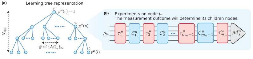
Fig. S1: (a) Learning tree representation. Each node $u$ represents an experiment. Starting from the root experiment $r$, the number of child nodes depends on the possible POVM measurements. The transition probabilities are determined by Equation 91. After $N_{\text{exp}}$ experiments, one arrives at the leaves $l$ of the learning tree. (b) In each node u, the learning model prepares an arbitrary state $\rho_{u}$, applies discrete control channels $\mathcal{C}^{u}_{k}$, and queries real-time Hamiltonian evolutions with time $\tau_{k}^{u}$ multiple times. The protocols can also incorporate ancilla qubits (quantum memory).

The high-level strategy of our proof is to combine the learning tree framework [50] equipped with the martingale trick [51, 52, 53] and quantum Fisher information.

Here, we generalize any experimental settings with discrete quantum controls and sequential queries to the Hamiltonian as the following theoretical model. Given a Hamiltonian $H$ with coefficient vector $\bm{\mu}$ defined in (1), the protocol performs multiple experiments as shown in Figure S1 and measures at the end of each experiment. In each experiment (indexed by $u$), the protocol prepares an input state $\rho_{u}$ (possibly with ancilla qubits) and queries the Hamiltonian $m_{u}$ times with evolution time $\tau_{1}^{u},...,\tau_{m_{u}}^{u}$. We can also apply discrete quantum control unitaries $\mathcal{C}_{1}^{u},...,\mathcal{C}_{m_{u}-1}^{u}$ between every two neighboring queries. The protocol can be adaptive in the sense that it can dynamically decide how to prepare the input state, query the real-time evolutions, perform quantum controls, and measure the final state based on the history of the previous experiments. We denote the summation of the evolution times for querying the Hamiltonian throughout all experiment to be the total evolution time $T$ and the maximal number of discrete quantum controls in one experiment as $\mathcal{L}$.

Formally, we describe the protocol scheme in Figure S1 as the learning tree model [50, 53] as follows:

Definition 5 (Learning tree representation).

Given a Hamiltonian $H(\bm{u})$ as defined in (90) with $M$ terms, a learning protocol using discrete control channels and queries to the Hamiltonian real-time evolutions as shown in Figure S1 can be represented as a rooted tree $\mathcal{T}$ of depth $N_{\exp}$ (corresponding to $N_{\exp}$ measurements) with each node representing the measurement outcome history so far. In addition, the following conditions are satisfied:

• We assign a probability $p^{\bm{\mu}}(u)$ for any node $u$ on the tree $\mathcal{T}$. The probability assigned to the root $r$ is $p^{\bm{\mu}}(r)=1$.

• At each non-leaf node $u$, we input the state $\rho_{u}$. By convexity, we can assume $\rho_{u}=\ket{\psi_{u}}\bra{\psi_{u}}$ a pure state. We then query $m_{t}$ rounds of real-time Hamiltonian evolution of time $\tau^{u}_{1},...,\tau^{u}_{m_{t}}$, interleaved with $m_{t}$ discrete control channels $\mathcal{C}_{1}^{u},...,\mathcal{C}_{m_{t}}^{u}$ (the last one, $\mathcal{C}_{m_{t}}^{u}$, can be absorbed into the measurement as shown in the figure). We then perform a POVM $\{\mathcal{M}_{s_{u}}^{u}\}_{s_{u}}$, which by the fact that any POVM can be simulated by rank-$1$ POVM [50], can be assumed to be a rank-$1$ POVM as $\{w^{u}_{s_{u}}\ket{\phi_{s_{u}}^{u}}\bra{\phi_{s_{u}}^{u}}\}_{s_{u}}$ with $\sum w^{u}_{s_{u}}=2^{n}$, and get classical output $s_{u}$. The child node $v$ corresponding to the classical outcome $s_{u}$ of the node $u$ is connected through the edge $e_{u,s_{u}}$. The probability associated with $v$ is given by:

  $$p^{\bm{\mu}}(v)\triangleq p^{\bm{\mu}}(u)\cdot\tr\left(w^{u}_{s_{u}}\ket{\phi_{s_{u}}^{u}}\bra{\phi_{s_{u}}^{u}}\cdot\mathcal{U}_{m_{u}}\mathcal{C}_{m_{u}-1}\mathcal{U}_{m_{u}-1}\cdots\mathcal{U}_{2}\mathcal{C}_{1}\mathcal{U}_{1}(\ket{\psi_{u}}\bra{\psi_{u}})\right),$$ (91)

  where $\mathcal{U}_{i}=e^{-iH(\bm{\mu})\tau_{i}}$ is the unitary real-time evolution of $H(\bm{\mu})$ for time $\tau_{i}$.

• Each root-to-leaf path is of length $N_{\exp}$. For a leaf node $\ell$, $p^{\bm{\mu}}(\ell)$ is the probability of reaching this leaf $\ell$ at the end of the learning protocol. The set of leaves is denoted as $\text{leaf}(\mathcal{T})$.

We consider a point-versus-point distinguishing task between two cases for a hyperparameter $\bm{\mu}$:

• The Hamiltonian for the real-time evolution is exactly $H(\bm{\mu})$.

• The Hamiltonian for the real-time evolution is actually $H(\bm{\mu}+\delta\bm{\mu})$ with $\norm{\delta\bm{\mu}}_{\infty}=3\epsilon$.

The goal is to distinguish which case is happening. It is straightforward to see that given an algorithm that can learn the Hamiltonian, we can solve this distinguishing problem.

Now, we consider how hard this distinguishing problem is. In the learning tree framework, the necessary condition for distinguishing between these two cases according to Le Cam’s two-point method [61] is that the total variation distance between the probability distributions on the leaves of the learning trees for the two cases is large. Quantitatively,

$$\begin{split}\frac{1}{2}\sum_{\ell\in\text{leaf}(\mathcal{T})}\absolutevalue{p^{\bm{\mu}+\delta\bm{\mu}}(\ell)-p^{\bm{\mu}}(\ell)}=\Theta(1).\end{split}$$ (92)

Using the martingale likelihood ratio argument developed by a series of works [51, 52, 62], the above lower bound can be converted to Lemma 7 of Ref. [53]: If there is a $\Delta>0$ such that

$$\mathbb{E}_{s_{u}\sim p^{\bm{\mu}}(s_{u}|u)}[(L_{\delta\bm{\mu}}(u,s_{u})-1)^{2}]\leq\Delta,$$ (93)

where

$$L_{\delta\bm{\mu}}(u,s_{u})=\frac{p^{\bm{\mu}+\delta\bm{\mu}}(s_{u}|u)}{p^{\bm{\mu}}(s_{u}|u)},$$ (94)

then $N_{\exp}\geq\Omega(1/\Delta)$. The physical intuition behind this result is that when the difference between the probability $p^{\bm{\mu}}(s_{u}|u)$ and the perturbed probability $p^{\bm{\mu}+\delta\bm{\mu}}(s_{u}|u)$ is very small across all levels of the learning tree (Equation 93), a very deep tree is required—i.e., $N_{\exp}\geq\Omega(1/\Delta)$ —to ensure that the measurement distributions at the leaf nodes are distinct (Equation 92).

Now, we focus on this quantity

$$\mathbb{E}_{s_{u}\sim p^{\bm{\mu}}(s_{u}|u)}[(L_{\delta\bm{\mu}}(u,s_{u})-1)^{2}]$$ (95)

for a specific $u$. Recall that $\norm{\delta\bm{\mu}}_{\infty}=3\epsilon$, we thus have $\norm{\delta\bm{\mu}}_{2}\leq 3\sqrt{M}\epsilon$. We can thus compute this quantity by extending it to the first-order term as

$$\begin{split}\mathbb{E}_{s_{u}\sim p^{\bm{\mu}}(s_{u}|u)}[(L_{\delta\bm{\mu}}(u,s_{u})-1)^{2}]&=\mathbb{E}_{s_{u}\sim p^{\bm{\mu}}(s_{u}|u)}\left[\left(\frac{p^{\bm{\mu}+\delta\bm{\mu}}(s_{u}|u)}{p^{\bm{\mu}}(s_{u}|u)}-1\right)^{2}\right]\\ &\simeq\mathbb{E}_{s_{u}\sim p^{\bm{\mu}}(s_{u}|u)}\left[\left(\frac{p^{\bm{\mu}}(s_{u}|u)+\nabla_{\bm{\mu}}p^{\bm{\mu}}(s_{u}|u)\cdot\delta\bm{\mu}}{p^{\bm{\mu}}(s_{u}|u)}-1\right)^{2}\right]\\ &=\mathbb{E}_{s_{u}\sim p^{\bm{\mu}}(s_{u}|u)}\left[\left(\frac{\nabla_{\bm{\mu}}p^{\bm{\mu}}(s_{u}|u)\cdot\delta\bm{\mu}}{p^{\bm{\mu}}(s_{u}|u)}\right)^{2}\right]\\ &=\delta\bm{\mu}^{\top}I^{(C)}_{\bm{\mu},u}\delta\bm{\mu}\\ &\leq\max_{\bm{v}:\norm{\bm{v}}_{2}\leq 3\sqrt{M}\epsilon}\bm{v}^{\top}I^{(C)}_{\bm{\mu},u}\bm{v},\end{split}$$ (96)

where

$$\begin{split}\left[I_{\bm{\mu},u}^{(C)}\right]_{a,a^{\prime}}&=\mathbb{E}_{s_{u}\sim p^{\bm{\mu}}(s_{u}|u)}\left[\left(\frac{\frac{\partial p^{\bm{\mu}}(s_{u}|u)}{\partial\lambda_{a}}}{p^{\bm{\mu}}(s_{u}|u)}\right)\left(\frac{\frac{\partial p^{\bm{\mu}}(s_{u}|u)}{\partial\lambda_{a^{\prime}}}}{p^{\bm{\mu}}(s_{u}|u)}\right)\right]\\ &=\mathbb{E}_{s_{u}\sim p^{{\bm{\mu}}}(s_{u}|u)}\left[\left(\frac{\partial\ln p^{\bm{\mu}}(s_{u}|u)}{\partial\lambda_{a}}\right)\left(\frac{\partial\ln p^{\bm{\mu}}(s_{u}|u)}{\partial\lambda_{a^{\prime}}}\right)\right]\end{split}$$ (97)

is the classical Fisher information matrix [47, 48, 49]. Note that quantum Fisher information $\bm{v}^{\top}I^{(Q)}_{{\bm{\mu}},u}\bm{v}$ is the supremum of classical Fisher information $\bm{v}^{\top}I^{(C)}_{{\bm{\mu}},u}\bm{v}$ over all possible measurements or observables [63]. By Lemma 17 of Ref. [46], assuming $H({\bm{\mu}})$ can be diagonalized as $H({\bm{\mu}})=W({\bm{\mu}})^{\dagger}D({\bm{\mu}})W({\bm{\mu}})$ with unitary $W$ and diagonal $D$, we have the quantum Fisher information satisfies

$$\max_{\bm{v}:\norm{\bm{v}}_{2}\leq 3\sqrt{M}\epsilon}\bm{v}^{\top}I^{(Q)}_{{\bm{\mu}},u}\bm{v}\leq M\epsilon^{2}\left(\min\left\{t_{u}\norm{\partial_{\bm{\mu}}D}_{\text{HS}}+2m_{u}\norm{\partial_{\bm{\mu}}W}_{\text{HS}},t_{u}\norm{\partial_{\bm{\mu}}H}_{\text{HS}}\right\}\right)^{2},$$ (98)

where $t_{u}=\sum_{i=1}^{m_{u}}\tau_{i}^{u}$ and $\norm{\cdot}_{\text{HS}}$ is the Hilbert Schmidt norm (spectral norm). By applying Eq. (93), we have

$$N_{\exp}=\Omega\left(\left(M\epsilon^{2}\left(\min\left\{2m_{u}\norm{\partial_{\bm{\mu}}W}_{\text{HS}},t_{u}\norm{\partial_{\bm{\mu}}H}_{\text{HS}}\right\}\right)^{2}\right)^{-1}\right)$$ (99)

for any protocols that can solve this distinguishing problem with a high probability. The RHS is maximized when $t_{u}\leq 2m_{u}\norm{\partial_{\bm{\mu}}W}_{\text{HS}}/\norm{\partial_{\bm{\mu}}H}_{\text{HS}}$. Denote $\mathcal{L}=\max_{u}m_{u}$ as the maximal number of discrete quantum controls in one experiment and $T=\sum_{u=1}^{N_{\text{exp}}}t_{u}$ as the total evolution time, we have

$$2M\epsilon^{2}\mathcal{L}T\norm{\partial_{\bm{\mu}}W}_{\text{HS}}\norm{\partial_{\bm{\mu}}H}_{\text{HS}}=\Theta(1),$$ (100)

which indicates that any protocol that can solve this distinguishing problem with a high probability requires $T=\Omega(\mathcal{L}^{-1}\epsilon^{-2})$ as claimed in Theorem 12 in the main text.

References

- Daley [2023] A. J. Daley, Twenty-five years of analogue quantum simulation, Nature Reviews Physics 5, 702 (2023).
- Bernien et al. [2017] H. Bernien, S. Schwartz, A. Keesling, H. Levine, A. Omran, H. Pichler, S. Choi, A. S. Zibrov, M. Endres, M. Greiner, V. Vuletić, and M. D. Lukin, Probing many-body dynamics on a 51-atom quantum simulator, Nature 551, 579 (2017).
- Semeghini et al. [2021] G. Semeghini, H. Levine, A. Keesling, S. Ebadi, T. T. Wang, D. Bluvstein, R. Verresen, H. Pichler, M. Kalinowski, R. Samajdar, A. Omran, S. Sachdev, A. Vishwanath, M. Greiner, V. Vuletić, and M. D. Lukin, Probing topological spin liquids on a programmable quantum simulator, Science 374, 1242 (2021), https://www.science.org/doi/pdf/10.1126/science.abi8794 .
- Ryan-Anderson et al. [2021] C. Ryan-Anderson, J. G. Bohnet, K. Lee, D. Gresh, A. Hankin, J. P. Gaebler, D. Francois, A. Chernoguzov, D. Lucchetti, N. C. Brown, T. M. Gatterman, S. K. Halit, K. Gilmore, J. A. Gerber, B. Neyenhuis, D. Hayes, and R. P. Stutz, Realization of real-time fault-tolerant quantum error correction, Phys. Rev. X 11, 041058 (2021).
- Postler et al. [2022] L. Postler, S. Heuβen, I. Pogorelov, M. Rispler, T. Feldker, M. Meth, C. D. Marciniak, R. Stricker, M. Ringbauer, R. Blatt, P. Schindler, M. Müller, and T. Monz, Demonstration of fault-tolerant universal quantum gate operations, Nature 605, 675 (2022).
- Bluvstein et al. [2024] D. Bluvstein, S. J. Evered, A. A. Geim, S. H. Li, H. Zhou, T. Manovitz, S. Ebadi, M. Cain, M. Kalinowski, D. Hangleiter, J. P. Bonilla Ataides, N. Maskara, I. Cong, X. Gao, P. Sales Rodriguez, T. Karolyshyn, G. Semeghini, M. J. Gullans, M. Greiner, V. Vuletić, and M. D. Lukin, Logical quantum processor based on reconfigurable atom arrays, Nature 626, 58 (2024).
- Google Quantum AI and Collaborators [2024] Google Quantum AI and Collaborators, Quantum error correction below the surface code threshold, Nature 10.1038/s41586-024-08449-y (2024).
- Zhou et al. [2024] H. Zhou, C. Zhao, M. Cain, D. Bluvstein, C. Duckering, H.-Y. Hu, S.-T. Wang, A. Kubica, and M. D. Lukin, Algorithmic Fault Tolerance for Fast Quantum Computing, arXiv e-prints , arXiv:2406.17653 (2024), arXiv:2406.17653 [quant-ph] .
- Carrasco et al. [2021] J. Carrasco, A. Elben, C. Kokail, B. Kraus, and P. Zoller, Theoretical and experimental perspectives of quantum verification, PRX Quantum 2, 010102 (2021).
- Hangleiter et al. [2024] D. Hangleiter, I. Roth, J. Fuksa, J. Eisert, and P. Roushan, Robustly learning the hamiltonian dynamics of a superconducting quantum processor, Nature Communications 15, 9595 (2024).
- Huang et al. [2023] H.-Y. Huang, Y. Tong, D. Fang, and Y. Su, Learning many-body hamiltonians with heisenberg-limited scaling, Phys. Rev. Lett. 130, 200403 (2023).
- Ma et al. [2024] M. Ma, S. T. Flammia, J. Preskill, and Y. Tong, Learning -body Hamiltonians via compressed sensing, arXiv e-prints , arXiv:2410.18928 (2024), arXiv:2410.18928 [quant-ph] .
- Li et al. [2024] H. Li, Y. Tong, T. Gefen, H. Ni, and L. Ying, Heisenberg-limited hamiltonian learning for interacting bosons, npj Quantum Information 10, 83 (2024).
- Ni et al. [2024] H. Ni, H. Li, and L. Ying, Quantum hamiltonian learning for the fermi-hubbard model, Acta Applicandae Mathematicae 191, 2 (2024).
- Bakshi et al. [2024] A. Bakshi, A. Liu, A. Moitra, and E. Tang, Structure learning of hamiltonians from real-time evolution, in 2024 IEEE 65th Annual Symposium on Foundations of Computer Science (FOCS) (IEEE, 2024) p. 1037–1050.
- Mirani and Hayden [2024] A. Mirani and P. Hayden, Learning interacting fermionic hamiltonians at the heisenberg limit, Phys. Rev. A 110, 062421 (2024).
- Stilck França et al. [2024] D. Stilck França, L. A. Markovich, V. V. Dobrovitski, A. H. Werner, and J. Borregaard, Efficient and robust estimation of many-qubit hamiltonians, Nature Communications 15, 311 (2024).
- Yu et al. [2023] W. Yu, J. Sun, Z. Han, and X. Yuan, Robust and Efficient Hamiltonian Learning, Quantum 7, 1045 (2023).
- Anshu et al. [2021] A. Anshu, S. Arunachalam, T. Kuwahara, and M. Soleimanifar, Sample-efficient learning of interacting quantum systems, Nature Physics 17, 931 (2021).
- Kokail et al. [2021] C. Kokail, R. van Bijnen, A. Elben, B. Vermersch, and P. Zoller, Entanglement hamiltonian tomography in quantum simulation, Nature Physics 17, 936 (2021).
- Olsacher et al. [2025] T. Olsacher, T. Kraft, C. Kokail, B. Kraus, and P. Zoller, Hamiltonian and liouvillian learning in weakly-dissipative quantum many-body systems, Quantum Science and Technology 10, 015065 (2025).
- Ott et al. [2024] R. Ott, T. V. Zache, M. Prüfer, S. Erne, M. Tajik, H. Pichler, J. Schmiedmayer, and P. Zoller, Hamiltonian Learning in Quantum Field Theories, arXiv e-prints , arXiv:2401.01308 (2024), arXiv:2401.01308 [cond-mat.quant-gas] .
- Caro [2024] M. C. Caro, Learning quantum processes and hamiltonians via the pauli transfer matrix, ACM Transactions on Quantum Computing 5, 10.1145/3670418 (2024).
- Möbus et al. [2023] T. Möbus, A. Bluhm, M. C. Caro, A. H. Werner, and C. Rouzé, Dissipation-enabled bosonic hamiltonian learning via new information-propagation bounds, arXiv preprint arXiv:2307.15026 (2023).
- Haah et al. [2022] J. Haah, R. Kothari, and E. Tang, Optimal learning of quantum hamiltonians from high-temperature gibbs states, in 2022 IEEE 63rd Annual Symposium on Foundations of Computer Science (FOCS) (2022) pp. 135–146.
- Bakshi et al. [2023] A. Bakshi, A. Liu, A. Moitra, and E. Tang, Learning quantum Hamiltonians at any temperature in polynomial time, arXiv e-prints , arXiv:2310.02243 (2023), arXiv:2310.02243 [quant-ph] .
- Gu et al. [2024] A. Gu, L. Cincio, and P. J. Coles, Practical hamiltonian learning with unitary dynamics and gibbs states, Nature Communications 15, 312 (2024).
- Qi and Ranard [2019] X.-L. Qi and D. Ranard, Determining a local Hamiltonian from a single eigenstate, Quantum 3, 159 (2019).
- Li et al. [2020] Z. Li, L. Zou, and T. H. Hsieh, Hamiltonian tomography via quantum quench, Phys. Rev. Lett. 124, 160502 (2020).
- Evans et al. [2019] T. J. Evans, R. Harper, and S. T. Flammia, Scalable Bayesian Hamiltonian learning, arXiv e-prints , arXiv:1912.07636 (2019), arXiv:1912.07636 [quant-ph] .
- Zhao [2024] A. Zhao, Learning the structure of any Hamiltonian from minimal assumptions, arXiv e-prints , arXiv:2410.21635 (2024), arXiv:2410.21635 [quant-ph] .
- Arunachalam et al. [2024] S. Arunachalam, A. Dutt, and F. Escudero Gutiérrez, Testing and learning structured quantum Hamiltonians, arXiv e-prints , arXiv:2411.00082 (2024), arXiv:2411.00082 [quant-ph] .
- Lidar [2012] D. A. Lidar, Review of Decoherence Free Subspaces, Noiseless Subsystems, and Dynamical Decoupling, arXiv e-prints , arXiv:1208.5791 (2012), arXiv:1208.5791 [quant-ph] .
- Choi et al. [2020] J. Choi, H. Zhou, H. S. Knowles, R. Landig, S. Choi, and M. D. Lukin, Robust dynamic hamiltonian engineering of many-body spin systems, Phys. Rev. X 10, 031002 (2020).
- Choi et al. [2017] S. Choi, N. Y. Yao, and M. D. Lukin, Dynamical engineering of interactions in qudit ensembles, Phys. Rev. Lett. 119, 183603 (2017).
- Evert et al. [2024] B. Evert, Z. Gonzalez Izquierdo, J. Sud, H.-Y. Hu, S. Grabbe, E. G. Rieffel, M. J. Reagor, and Z. Wang, Syncopated Dynamical Decoupling for Suppressing Crosstalk in Quantum Circuits, arXiv e-prints , arXiv:2403.07836 (2024), arXiv:2403.07836 [quant-ph] .
- Kimmel et al. [2015] S. Kimmel, G. H. Low, and T. J. Yoder, Robust calibration of a universal single-qubit gate set via robust phase estimation, Phys. Rev. A 92, 062315 (2015).
- Wallman and Emerson [2016] J. J. Wallman and J. Emerson, Noise tailoring for scalable quantum computation via randomized compiling, Phys. Rev. A 94, 052325 (2016).
- Emerson et al. [2007] J. Emerson, M. Silva, O. Moussa, C. Ryan, M. Laforest, J. Baugh, D. G. Cory, and R. Laflamme, Symmetrized characterization of noisy quantum processes, Science 317, 1893 (2007), https://www.science.org/doi/pdf/10.1126/science.1145699 .
- Chen et al. [2023a] S. Chen, Y. Liu, M. Otten, A. Seif, B. Fefferman, and L. Jiang, The learnability of pauli noise, Nature Communications 14, 52 (2023a).
- van den Berg et al. [2023] E. van den Berg, Z. K. Minev, A. Kandala, and K. Temme, Probabilistic error cancellation with sparse pauli–lindblad models on noisy quantum processors, Nature Physics 19, 1116 (2023).
- Hu et al. [2024] H.-Y. Hu, A. Gu, S. Majumder, H. Ren, Y. Zhang, D. S. Wang, Y.-Z. You, Z. Minev, S. F. Yelin, and A. Seif, Demonstration of Robust and Efficient Quantum Property Learning with Shallow Shadows, arXiv e-prints , arXiv:2402.17911 (2024), arXiv:2402.17911 [quant-ph] .
- Flammia and O’Donnell [2021] S. T. Flammia and R. O’Donnell, Pauli error estimation via Population Recovery, Quantum 5, 549 (2021).
- Campbell [2019] E. Campbell, Random compiler for fast hamiltonian simulation, Phys. Rev. Lett. 123, 070503 (2019).
- Chen et al. [2021] C.-F. Chen, H.-Y. Huang, R. Kueng, and J. A. Tropp, Concentration for random product formulas, PRX Quantum 2, 040305 (2021).
- Dutkiewicz et al. [2024] A. Dutkiewicz, T. E. O’Brien, and T. Schuster, The advantage of quantum control in many-body Hamiltonian learning, Quantum 8, 1537 (2024).
- Wootters [1981] W. K. Wootters, Statistical distance and hilbert space, Phys. Rev. D 23, 357 (1981).
- Braunstein and Caves [1994] S. L. Braunstein and C. M. Caves, Statistical distance and the geometry of quantum states, Phys. Rev. Lett. 72, 3439 (1994).
- Braunstein et al. [1996] S. L. Braunstein, C. M. Caves, and G. Milburn, Generalized uncertainty relations: Theory, examples, and lorentz invariance, Annals of Physics 247, 135 (1996).
- Chen et al. [2022] S. Chen, J. Cotler, H.-Y. Huang, and J. Li, Exponential separations between learning with and without quantum memory, in 2021 IEEE 62nd Annual Symposium on Foundations of Computer Science (FOCS) (2022) pp. 574–585.
- Chen et al. [2023b] S. Chen, J. Cotler, H.-Y. Huang, and J. Li, The complexity of nisq, Nature Communications 14, 6001 (2023b).
- Chen and Gong [2023] S. Chen and W. Gong, Efficient Pauli channel estimation with logarithmic quantum memory, arXiv e-prints , arXiv:2309.14326 (2023), arXiv:2309.14326 [quant-ph] .
- Chen et al. [2024] S. Chen, W. Gong, and Q. Ye, Optimal tradeoffs for estimating pauli observables, in 2024 IEEE 65th Annual Symposium on Foundations of Computer Science (FOCS) (2024) pp. 1086–1105.
- Zhou et al. [2018] S. Zhou, M. Zhang, J. Preskill, and L. Jiang, Achieving the heisenberg limit in quantum metrology using quantum error correction, Nature Communications 9, 78 (2018).
- Allen et al. [2025] R. R. Allen, F. Machado, I. L. Chuang, H.-Y. Huang, and S. Choi, Quantum Computing Enhanced Sensing, arXiv e-prints , arXiv:2501.07625 (2025), arXiv:2501.07625 [quant-ph] .
- Suzuki [1976] M. Suzuki, Generalized trotter’s formula and systematic approximants of exponential operators and inner derivations with applications to many-body problems, Communications in Mathematical Physics 51, 183 (1976).
- Suzuki [1977] M. Suzuki, On the convergence of exponential operators—the zassenhaus formula, bch formula and systematic approximants, Communications in Mathematical Physics 57, 193 (1977).
- Nakaji et al. [2024] K. Nakaji, M. Bagherimehrab, and A. Aspuru-Guzik, High-order randomized compiler for hamiltonian simulation, PRX Quantum 5, 020330 (2024).
- Childs et al. [2021] A. M. Childs, Y. Su, M. C. Tran, N. Wiebe, and S. Zhu, Theory of trotter error with commutator scaling, Phys. Rev. X 11, 011020 (2021).
- Note [1] By “non-adaptive” we mean that the choice of each does not depend on the value of or for any .
- Yu [1997] B. Yu, Assouad, Fano, and Le Cam, Festschrift for Lucien Le Cam: research papers in probability and statistics , 423 (1997).
- Chen and Brandão [2021] C.-F. Chen and F. G. S. L. Brandão, Fast Thermalization from the Eigenstate Thermalization Hypothesis, arXiv e-prints , arXiv:2112.07646 (2021), arXiv:2112.07646 [quant-ph] .
- Paris [2009] M. G. A. Paris, Quantum estimation for quantum technology, Int. J. Quantum Inf. 07, 125 (2009).