Stationary wave solutions to two dimensional viscous shallow water equations: theory of small and large solutions

Abstract.

We study a system of forced viscous shallow water equations with nontrivial bathymetry in two spatial dimensions. We develop a well-posedness theory for small but arbitrary forcing data, as well as for a fixed data profile but large amplitude. In the latter case, solutions may actually fail to exist for large amplitude, but in this case we prove that one of three physically meaningful breakdown scenarios occurs. Through the use of implicit function theorem techniques and a priori estimates, we construct both spatially periodic and solitary (non-periodic but spatially localized) solutions. The solitary case is substantially more complicated, requiring a delicate analysis in weighted Sobolev spaces. To the best of our knowledge, these results constitute the first general construction of stationary wave solutions, large or otherwise, to the viscous shallow water equations and the first general analysis of large solitary wave solutions to any viscous free boundary fluid model.

1. Introduction

1.1. The shallow water equations with applied force and bathymetry

In this paper we study a system of shallow water equations in two spatial dimensions that incorporates the effects of gravity, capillarity, viscosity, laminar drag, applied forces, and variable bathymetry (bottom topography):

$$\begin{cases}\partial_{t}h+\nabla\cdot((h-b)v)=0,\\ \partial_{t}((h-b)v)+\nabla\cdot((h-b)v\otimes v)+\alpha v-\mu\nabla\cdot((h-b)\mathbb{S}v)+(h-b)(g-\sigma\Delta)\nabla h={\upkappa}F,\\ F=\int_{b}^{h}f(\cdot,y)\;\mathrm{d}y+(h-b)\nabla(\varphi(\cdot,h))+(\varphi I-\Xi)(\cdot,h)\nabla h+\xi(\cdot,h).\end{cases}$$ (1.1)

Here the unknowns are the tangential fluid velocity field $v:\mathbb{R}^{+}\times\mathbb{R}^{2}\to\mathbb{R}^{2}$ and the fluid height $h:\mathbb{R}^{+}\times\mathbb{R}^{2}\to\mathbb{R}$. The bottom topography is modeled via the bathymetry function $b:\mathbb{R}^{2}\to\mathbb{R}$. We will always assume that the fluid height lies above the bathymetry, $h>b$, which means there are no ‘dry regions’. The coefficient of laminar friction is $\alpha\in\mathbb{R}^{+}$, the viscosity is $\mu\in\mathbb{R}^{+}$, and the shallow water viscous stress tensor is

$$\mathbb{S}v=\nabla v+\nabla v^{\mathrm{t}}+2(\nabla\cdot v)I.$$ (1.2)

The gravitational acceleration in the vertical direction is $g\geqslant 0$ and the surface tension coefficient is $\sigma\in\mathbb{R}^{+}$. The vector field $F:\mathbb{R}^{+}\times\mathbb{R}^{2}\to\mathbb{R}^{2}$, with units of length, is the profile of the forcing applied to the system while the coefficient $\upkappa\in\mathbb{R}$, with units of acceleration, indicates the strength of the applied forcing.

The system (1.1) is a viscous variant of the classical Saint-Venant equations ($\sigma=\mu={\upkappa}=0$). Its solutions approximate those of the free boundary incompressible Navier-Stokes system in the regimes in which either the fluid depth is very small or the solution has large characteristic wavelength. As a result, the model is physically, mathematically, and practically relevant in describing the flow of a thin fluid film over the graphical surface determined by $b$. For details of the derivation of (1.1) from the Navier-Stokes system see Appendix B.

There are formal similarities between system (1.1) and the barotropic compressible Navier-Stokes equations with density-dependent viscosity, in which $h-b$ and $v$ play the roles of the density and velocity, respectively. This correspondence dictates how we shall refer to the individual equations in the shallow water system. The first equation in (1.1) is dubbed the continuity equation, and it describes how the surface height $h$ is transported and stretched by flow. The second vector equation is called the momentum equation, and it asserts a balance of the advection term $\partial_{t}((h-b)v)+\nabla\cdot((h-b)v\otimes v)$ by the sum of laminar drag $-\alpha v$, dissipation $\mu\nabla\cdot((h-b)\mathbb{S}v)$, gravity-capillary effects $-(h-b)(g-\sigma\Delta)\nabla h$, and applied force ${\upkappa}F$. Notice that the role played by the bathymetry $b$ is only to modify the fluid depth $h-b$, which shows up as a sort of ‘variable coefficient’. We emphasize that system (1.1) is quasilinear and of mixed-type, as it involves both dissipative and hyperbolic-dispersive structures.

The third equation of (1.1) shows that the term $F$ is a function of both the bathymetry and the height. The precise form recorded there is derived by taking the shallow water limit of the free boundary Navier-Stokes equations acted on by a bulk force and surface stress. The function $f:\mathbb{R}^{+}\times\mathbb{R}^{3}\to\mathbb{R}^{2}$ is derived from the tangential part of the bulk force, while the functions $\varphi:\mathbb{R}^{+}\times\mathbb{R}^{3}\to\mathbb{R}$, $\Xi:\mathbb{R}^{+}\times\mathbb{R}^{3}\to\mathbb{R}^{2\times 2}_{\mathrm{sym}}$, and $\xi\in\mathbb{R}^{+}\times\mathbb{R}^{3}\to\mathbb{R}^{2}$ are pieces of a surface stress tensor. Again, we refer the reader to Appendix B for the precise details of the derivation.

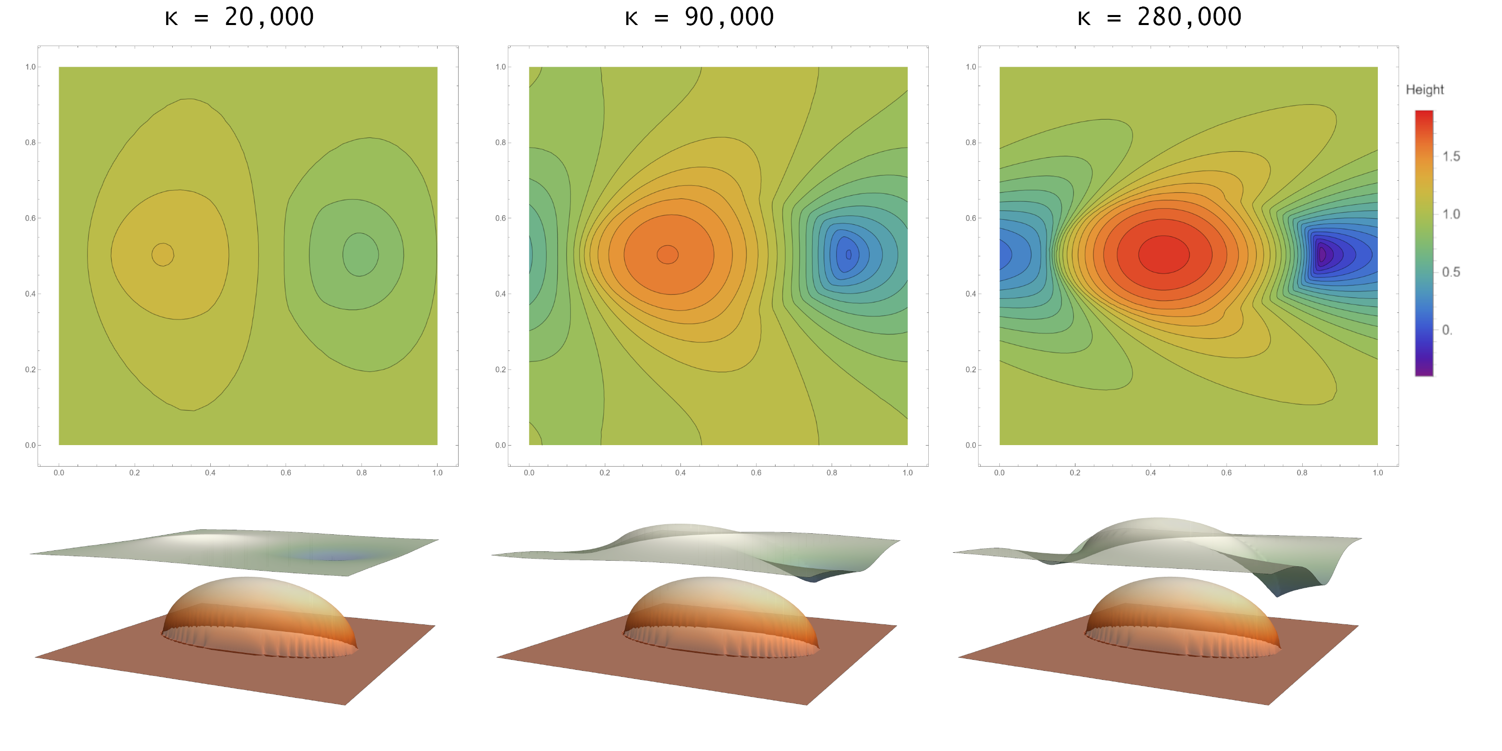
Figure 1. Depicted here are the height data from numerical simulations of periodic stationary solutions to (1.1), in contour plot form (top) and graph form (bottom), for three values of applied forcing strength ${\upkappa}\in\{{20000,90000,280000}\}$. The bathymetry $b$ (shown in orange on the bottom) is a fixed half-ellipse with base at height $-2$ and maximum at height $0$. The forcing profile $F$ is a component of gravity in the $e_{1}$ direction, i.e. $\varphi=0$, $\Xi=0$, $\xi=0$, and $f=e_{1}$. The surface satisfies $h=1+h_{0}$ for an average zero perturbation $h_{0}$. The other physical parameters are $\alpha=0.65$, $g=0.5$, $\mu=0.3$, and $\sigma=1.1$. This is meant to depict stationary shallow water flow over an inclined bathymetry.

Our principal goal in this paper is to develop a well-posedness theory for stationary (time independent) solutions to (1.1). We will construct both spatially periodic and non-periodic but localized and decaying solutions; we will refer to the former as the ‘periodic case’ and the latter as the ‘solitary case’. We will first construct small solutions for arbitrary data in a fixed open neighborhood of zero and then employ global implicit function theorem techniques to study how solutions behave as the amplitude of a fixed forcing profile is increased. In the latter case we will derive quantitative ‘alternatives’ that show that either the curves of solutions can be continued for all forcing data amplitudes or else degenerate in a specific, physically meaningful, manner.

Although we consider general $F$ of the form specified in (1.1), several specific choices warrant mentioning. One can model gravity-driven flow in the direction $\nu\in\mathbb{S}^{1}$ down an incline with the choice $F=(h-b)\nu$, i.e. $f=\nu$, $\varphi=0$, $\Xi=0$, and $\xi=0$. This scenario is depicted in Figures 1 and 2. On the other hand, the choice $F=(h-b)\nabla p$, which is achieved by $f=0$, $\varphi=p$, $\Xi=pI$, and $\xi=0$ for some scalar surface pressure $p:\mathbb{R}^{2}\to\mathbb{R}$, models a local change in pressure above the free surface.

1.2. Equilibria and stationary reformulation

We now aim to identify the equilibrium solutions to (1.1) and then reformulate (1.1) perturbatively about these equilibria in a nondimensional fashion. When $F=0$ and $b$ is a bounded function, the admissible steady solutions are constant and given by

$$v_{\mathrm{eq}}=0,\quad h_{\mathrm{eq}}=\mathrm{H}+\sup b\quad\text{for any choice of }\mathrm{H}\in\mathbb{R}^{+}.$$ (1.3)

Fixing an arbitrary choice of $\mathrm{H}\in\mathbb{R}^{+}$, we may nondimensionalize by selecting units with the effective normalization $(\mathrm{H},\mu,\sigma)\mapsto(1,1,1)$. This is a convenient choice, as positive viscosity and capillarity are crucial for our analytic techniques. Define the length and time

$$\mathrm{L}=\mu^{2}/\sigma,\quad\mathrm{T}=\mu^{3}/\sigma^{2}$$ (1.4)

and the new (negative) bathymetry $\beta$, velocity $\upupsilon$, and free surface height $\upeta$ as follows:

$$b(x)=\sup b-\mathrm{H}\beta(x/\mathrm{L}),\quad v(t,x)=(\mathrm{L}/\mathrm{T})\upupsilon(t/\mathrm{T},x/\mathrm{L}),\quad h(t,x)=\mathrm{H}(1+\upeta(t/\mathrm{T},x/\mathrm{L}))+\sup b.$$ (1.5)

In turn, define the new data profile $\Upphi$, inverse slip coefficient $A$, capillary number $G$, and inverse Froude number $\kappa$ via

$$F(t,x)=\mathrm{H}\Upphi(t/\mathrm{T},x/\mathrm{L}),\quad A=\frac{\alpha\mathrm{T}}{\mathrm{H}}=\frac{\alpha\mu^{3}}{\mathrm{H}\sigma^{2}},\quad G=\frac{g\mathrm{H}\mathrm{T}^{2}}{\mathrm{L^{2}}}=\frac{g\mathrm{H}\mu^{2}}{\sigma^{2}},\quad\kappa=\frac{{\upkappa}\mathrm{T}^{2}}{\mathrm{L}}=\frac{{\upkappa}\mu^{4}}{\sigma^{3}}.$$ (1.6)

Notice that $\beta\geqslant 0$ with $\inf\beta=0$; we work with the nonnegative quantity $\beta$ here for convenience, but one should think of $-\beta$ as the nondimensional description of the bathymetry. The positive fluid depth condition $h>b$ translates in these new variables to $1+\upeta+\beta>0$. In terms of the quantities (1.5) and (1.6), system (1.1) becomes

$$\begin{cases}\partial_{t}\upeta+\nabla\cdot((1+\beta+\upeta)\upupsilon)=0,\\ \partial_{t}((1+\beta+\upeta)\upupsilon)+\nabla\cdot((1+\beta+\upeta)\upupsilon\otimes\upupsilon)+A\upupsilon-\nabla\cdot((1+\beta+\upeta)\mathbb{S}\upupsilon)+(1+\beta+\upeta)(G-\Delta)\nabla\upeta=\kappa\Upphi.\end{cases}$$ (1.7)

As previously mentioned, our focus in this work is the not the full time dependent system (1.7), but rather the particular class of stationary (and thus global-in-time) solutions generated by generic time independent forcing. We are therefore led to make the stationary ansatz $\partial_{t}\upeta=0$, $\partial_{t}\upupsilon=0$, and $\partial_{t}\Upphi=0$, which we formulate for new stationary unknowns as $\upeta(t,x)=\boldsymbol{\eta}(x)$, $\upupsilon(t,x)=\boldsymbol{u}(x)$, and $\Upphi(t,x)=\Phi(x)$. In terms of the new unknowns, the system (1.7) becomes

$$\begin{cases}\nabla\cdot((1+\beta+\boldsymbol{\eta})\boldsymbol{u})=0,\\ \nabla\cdot((1+\beta+\boldsymbol{\eta})\boldsymbol{u}\otimes\boldsymbol{u})+A\boldsymbol{u}-\nabla\cdot((1+\beta+\boldsymbol{\eta})\mathbb{S}\boldsymbol{u})+(1+\beta+\boldsymbol{\eta})(G-\Delta)\nabla\boldsymbol{\eta}=\kappa\Phi.\end{cases}$$ (1.8)

The final form of the momentum equation source term $\Phi$ in (1.8), which we formally write as

$$\Phi=\phi(\cdot,\boldsymbol{\eta})+\nabla((1+\beta+\boldsymbol{\eta})\psi(\cdot,\boldsymbol{\eta}))+\tau(\cdot,\boldsymbol{\eta})\nabla\boldsymbol{\eta},$$ (1.9)

not only depends on $\boldsymbol{\eta}$ but also involves the generic functions $\phi:\mathbb{R}^{3}\to\mathbb{R}^{2}$, $\psi:\mathbb{R}^{3}\to\mathbb{R}$, and $\tau:\mathbb{R}^{3}\to\mathbb{R}^{2\times 2}_{\mathrm{sym}}$. This captures the general structure of the forcing present in the third equation of (1.1) after the rescaling and the stationary ansatz. See Section 1.4.1 for a more thorough discussion on these relationships.

We now discuss the necessity of nontrivial forcing in (1.8) for the generation of nontrivial solutions. As part of the proof of the later result Proposition 5.2, we establish the following power-dissipation identity for solutions to system (1.8) with trivial forcing ($\kappa=0$):

$$\int A|\boldsymbol{u}|^{2}+(1+\beta+\boldsymbol{\eta})(2^{-1}|\nabla\boldsymbol{u}+\nabla\boldsymbol{u}^{\mathrm{t}}|^{2}+2|\nabla\cdot\boldsymbol{u}|^{2})=0.$$ (1.10)

Here the domain of integration is understood as $\mathbb{R}^{2}$ when the solutions are solitary and as a fundamental domain when the solutions are periodic. When $A>0$ and $1+\beta+\boldsymbol{\eta}>0$, identity (1.10) implies that $\boldsymbol{u}=0$. In turn from (1.8) we may then deduce that $\nabla\boldsymbol{\eta}=0$, and hence the solution is trivial. This tells us that nontrivial solitary or periodic stationary solutions to (1.8) cannot exist unless they are generated by a nontrivial stationary applied force or stress, meaning $\kappa\Phi\neq 0$.

1.3. Previous work

A number of closely related variants of our shallow water system have been derived and studied in the literature: see, for instance [41, 50, 40, 25, 5, 6, 8, 36]. The model we employ is most similar to those derived in the articles of Marche [43], Bresch [9], and Mascia [44]; the article [9] also contains a very thorough survey of the dynamic problem for (1.1) and related models with flat bathymetry. As our paper’s focus is the stationary wave problem over smooth bottom topography, we will focus this literature review on work that accounts for bathymetry or studies time independent solutions.

Intimately related to the problem of stationary waves is that of traveling waves. Within the context of the shallow water equations (both inviscid and viscous) there is a large existing literature analyzing special types of one dimensional traveling waves down an incline, known as roll waves. Dressler [20] gives the first construction of discontinuous roll wave solutions to the inviscid Saint-Venant equations. Merkin and Needham [47, 46] augment to Dressler’s model an energy dissipation term and study the resulting roll waves; Hwang and Chang [28] provide further analyses. Chang, Cheng, and Prokopiou [53] include capillary effects and produce solitary roll waves. A complete theory of linear and nonlinear stability of one dimensional roll wave solutions to both the inviscid and viscous shallow water equations is developed in the works [32, 4, 3, 31, 56, 30]. The existence of two dimensional viscous gravity-capillary roll waves is addressed by Stevenson [60]. We also mention that Stevenson and Tice [61] establish the well-posedness for the small amplitude solitary traveling wave problem for system (1.1) over trivial bathymetry; however large or stationary waves were left unaddressed.

We next discuss the shallow water system with explicit bathymetric effects. To the best of our knowledge there are no results for our specific shallow water model (1.1); nevertheless, there are some results on related models. Cherevko and Chupakhin [15, 16] study shallow water equations on a rotating sphere and provide stationary solutions. De Valeriola and Van Schaftingen [18] study point vortex type stationary solutions and their desingularization within a system of shallow water equations with bathymetry called the lake equations; this is extended to multiple vortices by Cao and Liu [12]. Marangos and Porter [42] study linear shallow water theory over structured bathymetry. Ketcheson and Quezada de Luna [54] study the dispersive properties of linearized water waves over a periodic bathymetry and compare numerically with the Saint-Venant equations.

As the shallow water equations are derived from the free boundary incompressible Navier-Stokes equations, our work is also linked to the stationary and traveling wave problems for free boundary fluids. For the inviscid free boundary Euler equations, the water wave problem has been the target of intense study for well over a century. The interested reader is referred to the survey articles of Toland [66], Groves [26], Strauss [65], and Haziot, Hur, Strauss, Toland, Wahlén, Walsh, and Wheeler [27].

In contrast, the study of stationary and traveling wave solutions to viscous free boundary problems has only recently commenced. An essential feature of these variants of the problem is that waves are generated by the application of stationary or traveling external forces and stresses. For experimental studies regarding these types of traveling waves we refer, for instance, to the work of Akylas, Cho, Diorio, and Duncan [17, 19], Duncan and Masnadi [45], and Cho and Park [51, 52].

Leoni and Tice [39] give the first mathematical construction of strictly traveling wave solutions to the free boundary incompressible Navier-Stokes equations. This result is generalized by Stevenson and Tice [63, 62] to incompressible fluids with multiple layers and to compressible free boundary flows, and by Koganemaru and Tice [34, 35] to periodic or inclined fluids and flows obeying the Navier slip boundary condition. Nguyen and Tice [49] construct traveling wave solutions to free boundary Darcy flow and, in the periodic case, analyze their stability. The existence of solitary stationary waves requires more difficult analysis than the strictly traveling cases; Stevenson and Tice [64] give the first construction of solitary stationary traveling wave solutions to the free boundary incompressible Navier-Stokes system. All of the aforementioned results on stationary and traveling waves in viscous fluids regard small amplitude solutions. The first general constructions of large amplitude traveling wave solutions are carried out by Nguyen [48] and Brownfield and Nguyen [10] for free boundary Darcy flow.

Within the context of these previous results on viscous traveling and stationary waves, one sees that the current paper furthers the theory by settling two outstanding questions about the shallow water system. First, in the case of both Reynolds and Bond numbers finite we resolve the problem of well-posedness for small amplitude stationary waves. Second, we provide the first study of generic large stationary wave solutions, further expanding the study of viscous traveling wave problems past the realm of small solutions. Another key feature of our results is that we handle both the cases of periodic and solitary waves. For the latter case our work stands as the first construction of large solitary waves solutions within the viscous stationary and traveling wave problem literature.

1.4. Main results, discussion, and outline

We now come to the statement of our main theorems, the proofs of which can be found in Section 6. Our results split into two categories based on whether we assume the solutions are periodic or not, with the latter case resulting in spatially localized solitary waves. Within each category we prove two results, one on small solutions and one on large solutions. The former establishes the well-posedness of the system (1.8) with a fixed bathymetry $\beta$ and $\kappa=1$, and forcing $\Phi$ generic and small (near $0$). The large data result then explores what happens for a fixed but arbitrary choice of forcing data profile but variable forcing strength $\kappa\in\mathbb{R}$. Before stating any of these, a discussion of how we handle the forcing term $\Phi$ in (1.8) is required.

1.4.1. Data technicalities

Equation (1.9) shows that the forcing profile $\Phi$ of the second equation in (1.8) depends nonlinearly on the free surface function $\boldsymbol{\eta}$. As we discuss in Appendix B, this dependence is not arbitrary and has a specific functional form $\boldsymbol{\eta}\mapsto\Phi$ derived from the base free boundary Navier-Stokes system. In specifying this dependence we run into some technical issues that merit discussion.

The first issue we encounter is that we would like to impose just enough regularity on $\Phi$ to produce strong solutions, say $\boldsymbol{u}\in H^{2}_{\mathrm{loc}}(\mathbb{R}^{2};\mathbb{R}^{2})$ and $\boldsymbol{\eta}\in H^{3}_{\mathrm{loc}}(\mathbb{R}^{2})$ with $\Phi\in L^{2}_{\mathrm{loc}}(\mathbb{R}^{2};\mathbb{R}^{2})$. Given that $\Phi$ contains terms of the form $\phi(\cdot,\boldsymbol{\eta})$, we then run into the usual headache of dealing with (partial) composition with maps that are no better than measurable on a product. Of course, this is an old problem, and a typical solution is to force the maps defining $\Phi$ to be Carathéodory functions, which imposes a.e. continuity in the second variable.

The second issue is that we aim to produce solutions with the implicit function theorem for maps between Banach spaces: the standard local one for small solutions, and a specialized global one for large solutions. At a minimum, this requires continuous differentiability for the (Nemytskii) map $\mathcal{X}\supseteq U\ni\boldsymbol{\eta}\mapsto\Phi\in\mathcal{Y}$, where $\mathcal{X}$ and $\mathcal{Y}$ are (to be determined) Banach spaces of functions and $U\subseteq\mathcal{X}$ is an open set. Again, this is not a new problem, and one solution is to impose enough regularity on the maps defining the dependence of $\Phi$ on $\boldsymbol{\eta}$ to invoke some version of the omega lemma (e.g. Lemma 2.4.18 in [1], or the main results of [29]) to get the needed continuous differentiability between $\mathcal{X}$ and $\mathcal{Y}$. For example, for the component term $\boldsymbol{\eta}\mapsto\phi(\cdot,\boldsymbol{\eta})$ we would expect to need $\phi$ to be at least continuously differentiable in its second argument, surpassing the Carathéodory mandate.

It turns out that the nonlinear structure of (1.8) allows us to formulate solutions as the zeros of a real analytic map between Banach spaces. Exploiting this analytic structure is advantageous, as it allows us to employ an analytic global implicit function theorem of Chen, Walsh, and Wheeler [14] (see also Theorem 5.1 below), which gives us stronger information than other global implicit function theorems (e.g. Section II.6 in [33]). Furthermore, real analyticity also presents a convenient, if somewhat tricky to explain, mechanism for dealing with the above two issues. We now aim to explain our technique by focusing on the simple case $\Phi=\phi(\cdot,\boldsymbol{\eta})$.

Fix the map $\phi:\mathbb{R}^{2}\times I\to\mathbb{R}^{2}$ for some interval $I\subseteq\mathbb{R}$. The discussion above suggests that we want $\phi(\cdot,\boldsymbol{\eta})\in\mathcal{Y}\hookrightarrow L^{2}_{\mathrm{loc}}(\mathbb{R}^{2};\mathbb{R}^{2})$ and the map $\mathcal{X}\supseteq U\ni\boldsymbol{\eta}\mapsto\phi(\cdot,\boldsymbol{\eta})\in\mathcal{Y}$ to be real-analytic. This is relatively easy to do if we assume that $\phi$ has a special structure. Indeed, if we assume $\phi$ is continuous and a polynomial in its final variable, say $\phi(x,y)=\sum_{j=0}^{\ell}g_{j}(x)y^{j}$ for $g_{j}\in C^{0}(\mathbb{R}^{2};\mathbb{R}^{2})\cap\mathcal{Y}$, then the pointwise evaluation $\Phi(x)=\phi(x,\boldsymbol{\eta}(x))$ presents no trouble if we assume $\boldsymbol{\eta}\in\mathcal{X}$ for $\mathcal{X}$ a unital Banach subalgebra of $(C^{0}\cap L^{\infty})(\mathbb{R}^{2};\mathbb{R})$, and we can obtain analyticity of the map $\boldsymbol{\eta}\mapsto\Phi$ by noting that $\mathcal{X}\ni\boldsymbol{\eta}\mapsto\sum_{j=0}^{\ell}g_{j}\boldsymbol{\eta}^{j}\in\mathcal{Y}$ is analytic when $\mathcal{X}\hookrightarrow\mathcal{L}(\mathcal{Y})$ via the pointwise product.

This special polynomial form of $\phi$ is too restrictive, but the analysis presents a natural generalization. We first Curry the map $\phi$ in its second argument to think of $\phi(x,y)=\hat{\phi}(y)(x)$ for a given analytic map $\hat{\phi}:I\to\mathcal{Y}$. There is now some technical hassle in making sense of the formal diagonal composition $\mathbb{R}^{2}\ni x\mapsto\hat{\phi}(\boldsymbol{\eta}(x))(x)\in\mathbb{R}^{2}$ in the general cases in which we only have the embedding $\mathcal{Y}\hookrightarrow L^{2}_{\mathrm{loc}}(\mathbb{R}^{2};\mathbb{R}^{2})$ and pointwise evaluation is discontinuous. We circumvent this issue and more in Appendix A.1 by developing a variant of the holomorphic functional calculus that allows us to uniquely (subject to some mild technical assumptions) define a ‘Nemytskii map’ $\Upomega_{\hat{\phi}}(\boldsymbol{\eta})\in\mathcal{Y}$ in such a way that the function $\mathcal{X}\supseteq U\ni\boldsymbol{\eta}\mapsto\Upomega_{\hat{\phi}}(\boldsymbol{\eta})\in\mathcal{Y}$ is analytic and also satisfies: $\Upomega_{\hat{\phi}}(\boldsymbol{\eta})=\sum_{j=0}^{\ell}g_{j}\boldsymbol{\eta}^{j}$ whenever $\hat{\phi}(y)=\sum_{j=0}^{\ell}g_{j}y^{j}$ is a polynomial with $g_{j}\in\mathcal{Y}$; and $[{\Upomega_{\hat{\phi}}(\boldsymbol{\eta})}](x)=\hat{\phi}(\boldsymbol{\eta}(x))(x)$ for $x\in\mathbb{R}^{2}$ when $\mathcal{Y}\hookrightarrow C^{0}_{\mathrm{loc}}(\mathbb{R}^{2};\mathbb{R}^{2})$.

The upshot of this discussion is that in the following theorem statements we will take $\Phi$ in (1.8), whose formal expression we initially gave as (1.9), to be rigorously defined as

$$\Phi=\Upomega_{\phi}(\boldsymbol{\eta})+\nabla((1+\beta+\boldsymbol{\eta})\Upomega_{\psi}(\boldsymbol{\eta}))+\Upomega_{\tau}(\boldsymbol{\eta})\nabla\boldsymbol{\eta}$$ (1.11)

where $\Upomega$ is the Nemytskii map constructed by the holomorphic function calculus in Appendix A.1 as described above, and $\phi$, $\psi$, $\tau$ are generically selected real analytic maps defined on an interval subset of the real line with values in certain Banach spaces of locally square summable functions.

1.4.2. Results for periodic functions

Our first two theorems consider solutions to system (1.8) in spaces of periodic functions. We fix a tuple of period lengths $L=(L_{1},L_{2})\in(\mathbb{R}^{+})^{2}$ and let $\mathbb{T}^{2}_{L}=(L_{1}\mathbb{T})\times(L_{2}\mathbb{T})$ denote the $2$-torus of side lengths $L_{1}$ and $L_{2}$. Given any $s\in\mathbb{N}$ and a finite dimensional real vector space $V$ we let $H^{s}(\mathbb{T}^{2}_{L};V)$ denote the standard Sobolev space of $V$-valued $L$-periodic functions; also we let $\mathring{H}^{s}(\mathbb{T}^{2}_{L};V)\subset H^{s}(\mathbb{T}^{2}_{L};V)$ denote the closed subspace of functions with vanishing mean.

To properly state our first theorem on small periodic solutions, we now need to specify the appropriate Banach space for the data $\phi$, $\psi$, and $\tau$ of (1.11) (whose role is discussed in Section 1.4.1). The precise definition is a bit technical (see Section 6.1, and in particular equation (6.1)), so for now we shall content ourselves with denoting the data space

$$\boldsymbol{Y}(\mathbb{T}^{2}_{L})=\boldsymbol{A}(L^{2}(\mathbb{T}^{2}_{L};\mathbb{R}^{2}))\times\boldsymbol{A}(H^{1}(\mathbb{T}^{2}_{L}))\times\boldsymbol{A}(L^{2}(\mathbb{T}^{2}_{L};\mathbb{R}^{2\times 2}_{\mathrm{sym}}))$$ (1.12)

and mentioning that $\boldsymbol{A}(\mathcal{Y})$, for $\mathcal{Y}\in\{{L^{2}(\mathbb{T}^{2}_{L};\mathbb{R}^{2}),H^{1}(\mathbb{T}^{2}_{L}),L^{2}(\mathbb{T}^{2}_{L};\mathbb{R}^{2\times 2}_{\mathrm{sym}})}\}$, is a Banach space of $\mathcal{Y}-$valued real analytic functions defined on a real interval, containing at least every entire function.

Theorem 1 (Proved in Theorem 6.2).

Let $\beta\in C^{\infty}(\mathbb{T}^{2}_{L})$ satisfy $\min\beta=0$, $A>0$, and $G\geqslant 0$. There exists positive radii $r_{\mathrm{soln}},r_{\mathrm{data}}\in\mathbb{R}^{+}$ and nonempty open balls $B_{\mathrm{data}}=B(0,r_{\mathrm{data}})\subset\boldsymbol{Y}(\mathbb{T}^{2}_{L})$ and $B_{\mathrm{soln}}=B(0,r_{\mathrm{soln}})\subset H^{2}(\mathbb{T}^{2}_{L};\mathbb{R}^{2})\times\mathring{H}^{3}(\mathbb{T}^{2}_{L})$ with the property that for all $(\phi,\psi,\tau)\in B_{\mathrm{data}}$ there exists a unique $(\boldsymbol{u},\boldsymbol{\eta})\in B_{\mathrm{soln}}$ solving the system of equations (1.8) with $\kappa=1$ and $\Phi$ determined by (1.11). Moreover, the mapping $(\phi,\psi,\tau)\mapsto(\boldsymbol{u},\boldsymbol{\eta})$ is real analytic.

Theorem 1 establishes the well-posedness of equations (1.8) in the class of small amplitude and periodic functions. Our next main result studies large solutions in the periodic setting. In this case we make some further (mild) restrictions on the data: we require a bit more smoothness on the $\tau$ component and that the domain of analyticity is unbounded from above (so that the composition with tall free surfaces $\boldsymbol{\eta}$ is well-defined). The hypotheses on the bathymetry $\beta$ are the same as in Theorem 1.

Theorem 2 (Proved in Theorem 6.3).

Let $\beta\in C^{\infty}(\mathbb{T}^{2}_{L})$ satisfy $\min\beta=0$, $A>0$, and $G\geqslant 0$. Set $a_{\beta}=1+\max\beta$, fix any choice of real analytic functions

$$(\phi,\psi,\tau):(-a_{\beta},\infty)\to L^{2}(\mathbb{T}^{2}_{L};\mathbb{R}^{2})\times H^{1}(\mathbb{T}^{2}_{L})\times(L^{\infty}\cap H^{1})(\mathbb{T}^{2}_{L};\mathbb{R}^{2\times 2}_{\mathrm{sym}}),$$ (1.13)

and define the set of admissible solutions (corresponding to the above fixed data profile and variable forcing strength) as

$$\boldsymbol{S}=\{{(\boldsymbol{u},\boldsymbol{\eta},\kappa)\in H^{2}(\mathbb{T}^{2}_{L};\mathbb{R}^{2})\times\mathring{H}^{3}(\mathbb{T}^{2}_{L})\times\mathbb{R}\;:\;\min(1+\beta+\boldsymbol{\eta})>0,\;\text{system~\eqref{stationary nondimensionalized equations} is satisfied with~\eqref{percolate propane pulvarized paintbrush}}}\}.$$ (1.14)

Then there exists a locally analytic curve $\mathscr{S}\subseteq\boldsymbol{S}$, with $0\in\mathscr{S}$, that is parametrized by the continuous mapping $\mathbb{R}\ni s\mapsto(\boldsymbol{u}(s),\boldsymbol{\eta}(s),\kappa(s))\in\mathscr{S}$ and satisfies $0\mapsto 0$ as well as the limits

$$\lim_{|s|\to\infty}\Big{[}{\lVert\boldsymbol{\eta}(s)\rVert_{L^{\infty}}+\frac{1}{\min(1+\beta+\boldsymbol{\eta}(s))}+|\kappa(s)|}\Big{]}=\infty.$$ (1.15)

Note that in Theorems 1 and 2 the periodicity allows us to set the nondimensionalized constant $G=0$; as one can see from the definition in (1.6), this can occur due to vanishing gravitational field or other ratios vanishing. The limits (1.15) indicate that for a fixed forcing profile, either there are solutions in $\mathscr{S}$ for an unbounded set of forcing amplitudes $\kappa$, or else $\kappa$ remains bounded but the solutions degenerate by the free surface touching the bottom or diverging in supremum norm. See Figures 1 and 2 for depictions of some of the periodic solutions considered by Theorem 2.

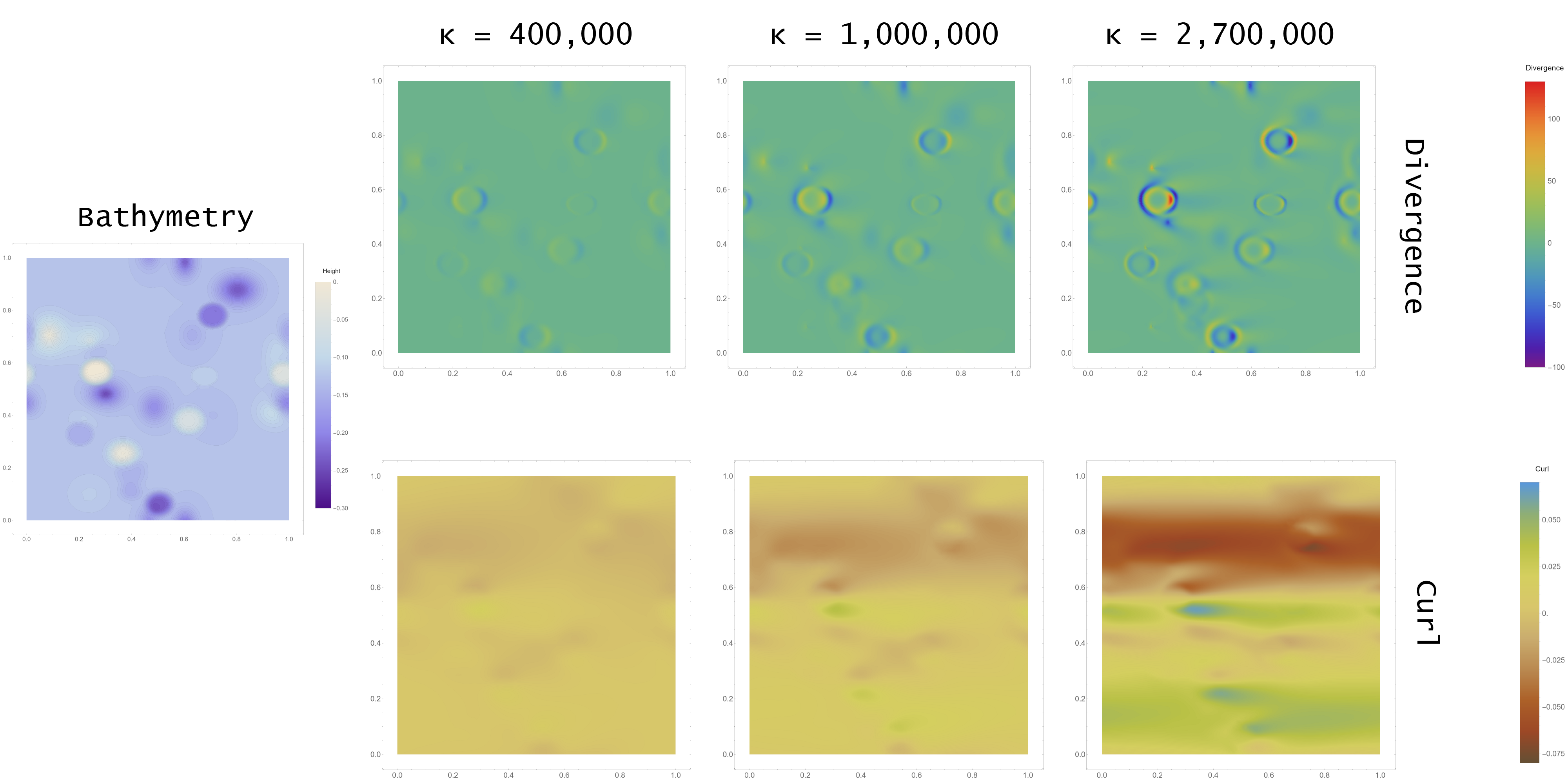
Figure 2. Shown here are are numerical simulations of the divergence (top row) and curl (bottom row) of the tangential velocity $v$ of gravity driven shallow water flow over a fixed, but randomly generated bathymetry $b$ (shown on the left). These correspond to stationary solutions to system (1.1) with forcing $F$ determined by $f=e_{1}$, $\varphi=0$, $\Xi=0$, and $\xi=0$. The forcing strength varies in the set ${\upkappa}\in\{{400000,1000000,2700000}\}$ while the other parameters $\alpha$, $g$, $\mu$, $\sigma$, and equilibrium height are all set to $1$.

1.4.3. Results for solitary functions

Our final two main results are the analogs of Theorems 1 and 2 but in solitary (i.e. decaying at infinity) function spaces. The functional framework becomes significantly more complicated due to the fact that in this setting we must overcome a certain low-mode degeneracy in the estimates for the free surface. We achieve this by working with Sobolev spaces built on weighted Lebesgue spaces. The full details of these function spaces can be found in Sections 2.1 and 2.2, but for now we shall content ourselves with the following abbreviated definitions. Given $1\leqslant q\leqslant\infty$, $0<\delta<1$, and a finite dimensional real vector space $V$, we let $L^{q}_{\delta}(\mathbb{R}^{2};V)$ denote the set of $f\in L^{q}(\mathbb{R}^{2};V)$ for which $\langle X\rangle^{\delta}f\in L^{q}(\mathbb{R}^{2};V)$, where $X:\mathbb{R}^{2}\to\mathbb{R}^{2}$ denotes the identity map and $\langle\cdot\rangle$ is the bracket (1.25). Given $s\in\mathbb{N}$, we then define the weighted Sobolev space $W^{s,q}_{\delta}(\mathbb{R}^{2};V)$ to be the collection of $f\in L^{q}_{\delta}(\mathbb{R}^{2};V)$ such that for all multiindices $|\alpha|\leqslant s$ we have $\partial^{\alpha}f\in L^{q}_{\delta}(\mathbb{R}^{2};V)$. When $q=2$ we write $H^{s}_{\delta}(\mathbb{R}^{2};V)$ in place of $W^{s,2}_{\delta}(\mathbb{R}^{2};V)$.

These weighted Sobolev spaces are appropriate container spaces for the velocity $\boldsymbol{u}$ and the data, but they are not quite adequate for the free surface function $\boldsymbol{\eta}$. For it we also need to introduce the weighted gradient Sobolev spaces, denoted by $\widetilde{H}^{s}_{\delta}(\mathbb{R}^{2})$ for $s\in\mathbb{N}^{+}$ and $0<\delta<1$, and consisting of $f\in L^{2/\delta}(\mathbb{R}^{2})$ with $\nabla f\in H^{s-1}_{\delta}(\mathbb{R}^{2};\mathbb{R}^{2})$, normed by the latter inclusion. These spaces satisfy the embeddings $H^{s}_{\delta}(\mathbb{R}^{2})\hookrightarrow\widetilde{H}^{s}_{\delta}(\mathbb{R}^{2})\hookrightarrow(H^{s}_{\delta}+W^{\infty,2/\delta})(\mathbb{R}^{2})$.

The solitary case necessitates imposing some admissibility conditions on the bathymetry profile $\beta$. Namely, we need its derivatives to be localized, which we impose by assuming that there exists $\delta\in(0,1)$ such that

$$\beta\in C^{\infty}(\mathbb{R}^{2}),\;\nabla\beta\in H^{\infty}_{\delta}(\mathbb{R}^{2};\mathbb{R}^{2}),\;\text{and}\;\inf\beta=0.$$ (1.16)

We now come to our third main theorem, which considers small solitary solutions. In place of (1.12), the solitary data space is

$$\boldsymbol{Y}(\mathbb{R}^{2})=\boldsymbol{A}(L^{2}_{\scriptscriptstyle 1/2}(\mathbb{R}^{2};\mathbb{R}^{2}))\times\boldsymbol{A}(H^{1}_{\scriptscriptstyle 1/2}(\mathbb{R}^{2}))\times\boldsymbol{A}(L^{2}_{\scriptscriptstyle 1/2}(\mathbb{R}^{2};\mathbb{R}^{2\times 2}_{\mathrm{sym}})),$$ (1.17)

whose precise definition is given at the start of Section 6.1.

Theorem 3 (Proved in Theorem 6.2).

Let $\beta$ be as in (1.16), $A>0$, and $G>0$. There exists positive radii $\rho_{\mathrm{soln}},\rho_{\mathrm{data}}\in\mathbb{R}^{+}$ and nonempty open balls $B_{\mathrm{data}}=B(0,\rho_{\mathrm{data}})\subset\boldsymbol{Y}(\mathbb{R}^{2})$ and $B_{\mathrm{soln}}=B(0,\rho_{\mathrm{soln}})\subset H^{2}_{\scriptscriptstyle 1/2}(\mathbb{R}^{2};\mathbb{R}^{2})\times\widetilde{H}^{3}_{\scriptscriptstyle 1/2}(\mathbb{R}^{2})$ with the property that for all $(\phi,\psi,\tau)\in B_{\mathrm{data}}$ there exists a unique $(\boldsymbol{u},\boldsymbol{\eta})\in B_{\mathrm{soln}}$ solving (1.8) with $\kappa=1$ and $\Phi$ determined by (1.11). Moreover, the mapping $(\phi,\psi,\tau)\mapsto(\boldsymbol{u},\boldsymbol{\eta})$ is real analytic.

Theorem 3 establishes the well-posedness of equations (1.8) in a class of small amplitude and solitary functions. Our final main theorem examines large solutions in the solitary case. As in the periodic case, we make some further minor restrictions on the class of data considered.

Theorem 4 (Proved in Theorem 6.3).

Let $\beta$ be as in (1.16), $A>0$, and $G>0$. Set $a_{\beta}=1+\sup\beta$, fix any choice of real analytic functions

$$(\phi,\psi,\tau):(-a_{\beta},\infty)\to L^{2}_{\scriptscriptstyle 1/2}(\mathbb{R}^{2};\mathbb{R}^{2})\times H^{1}_{\scriptscriptstyle 1/2}(\mathbb{R}^{2})\times(L^{\infty}_{\scriptscriptstyle 1/2}\cap H^{1}_{\scriptscriptstyle 1/2})(\mathbb{R}^{2};\mathbb{R}^{2\times 2}_{\mathrm{sym}}),$$ (1.18)

and define the set of admissible solutions (corresponding to the above fixed data profile and variable forcing strength) as

$$\boldsymbol{S}=\{{(\boldsymbol{u},\boldsymbol{\eta},\kappa)\in H^{2}_{\scriptscriptstyle 1/2}(\mathbb{R}^{2};\mathbb{R}^{2})\times\widetilde{H}^{3}_{\scriptscriptstyle 1/2}(\mathbb{R}^{2})\times\mathbb{R}\;:\;\inf(1+\beta+\boldsymbol{\eta})>0,\;\text{system~\eqref{stationary nondimensionalized equations} with~\eqref{percolate propane pulvarized paintbrush} is satisfied}}\}.$$ (1.19)

There exists a locally analytic curve $\mathscr{S}\subseteq\boldsymbol{S}$, with $0\in\mathscr{S}$, that is parametrized by the continuous mapping $\mathbb{R}\ni s\mapsto(\boldsymbol{u}(s),\boldsymbol{\eta}(s),\kappa(s))\in\mathscr{S}$ and satisfies $0\mapsto 0$ as well as the limits

$$\lim_{|s|\to\infty}\Big{[}{\lVert\boldsymbol{\eta}(s)\rVert_{L^{\infty}}+\min\{{\lVert\boldsymbol{u}(s)\rVert_{L^{q}},\lVert\boldsymbol{\eta}(s)\rVert_{L^{r}}}\}+\frac{1}{\inf(1+\beta+\boldsymbol{\eta}(s))}+|\kappa(s)|}\Big{]}=\infty$$ (1.20)

for every choice of $q\in(4/3,2)$ and $r\in[4,\infty)$.

Note that in the stationary case we must set $G>0$ to produce solutions. Again, the limits (1.20) indicate that either solutions exist for an unbounded set of $\kappa$, or else they degenerate in a particular way. The blowup scenarios from the periodic case remain but are augmented with a new option: the blowup of $\min\{{\lVert\boldsymbol{u}(s)\rVert_{L^{q}},\lVert\boldsymbol{\eta}(s)\rVert_{L^{r}}}\}\to\infty$ when $\limsup_{s\to\pm\infty}\lVert\boldsymbol{\eta}(s)\rVert_{L^{\infty}}<\infty$, which indicates a sort of delocalization of both the velocity and free surface functions. We included this new option for purely technical reasons stemming from the a priori estimates developed in Proposition 5.7; in principle, it might be possible to rule out this scenario by improving this proposition, but at the moment we lack the tools to do so.

1.4.4. Discussion of techniques

We now turn to a discussion of our techniques for proving the main theorems. At the highest level of abstraction, our general methods are the same in the periodic and solitary cases; what differs between the cases is the precise reformulation of (1.8) and the specific functional framework. The main goal in reformulating the equations is to semilinearize them, which we take to mean rewrite abstractly as

$$P\Xi=N(\Xi)+\kappa F(\Xi)$$ (1.21)

for an unknown $\Xi$, $P$ a linear differential operator, $N$ a nonlinear map acting at lower order than $P$, and $F$ given data also acting at lower order. We aim to do this in such a way that the operator $P$ is invertible, which then allows for the abstract fixed-point reformulation

$$(I+\mathcal{K})(\Xi)=\Xi+\mathcal{K}(\Xi)=\kappa\mathcal{F}(\Xi)\text{ for }\mathcal{K}=P^{-1}\circ N\text{ and }\mathcal{F}=P^{-1}\circ F.$$ (1.22)

The global implicit function theorems (GIFT) we are aware of all require some form of Fredholm condition on the derivative of the nonlinear map, and the $I+\mathcal{K}$ functional form above is convenient for verifying this by checking that $\mathcal{K}$ is a compact map. Moreover, this form lets us readily eliminate a number of the alternatives provided by the particular GIFT we use (see Theorem 5.1). The specific forms of $P$ and $N$ (and thus $\mathcal{K}$) differ in the periodic and solitary cases for a number of technical reasons, which we now discuss.

In both cases we assume that the fluid depth $1+\beta+\boldsymbol{\eta}$ is everywhere positive, which is convenient in that it permits us to arrive at systems equivalent to (1.8) by dividing each equation by the fluid depth. Once this is done for the momentum equation, one notices that the highest order term for $\boldsymbol{u}$ is $\nabla\cdot\mathbb{S}\boldsymbol{u}$, while the highest order term for $\boldsymbol{\eta}$ is $-\Delta\nabla\boldsymbol{\eta}$. As these are both linear, we have successfully semilinearized the momentum equation. Unfortunately, this procedure does not so nicely semilinearize the continuity equation. The problem is that, while the top order contribution is indeed the linear term $\nabla\cdot\boldsymbol{u}$, the function space in which the equation must hold is a subset of the range of the divergence and hence is not closed under multiplication by smooth functions. Fortunately, in the periodic case there is a simple workaround for this issue: in Lemma 3.3 we establish that the continuity equation of (1.8) holds if and only if

$$\nabla\cdot\boldsymbol{u}+P_{0}(\boldsymbol{u}\cdot\nabla\log(1+\beta+\boldsymbol{\eta}))=0,$$ (1.23)

where $P_{0}$ is the projection onto the space of mean-zero functions. Equation (1.23) is a valid semilinear reformulation of the continuity equation that respects the target space. Unfortunately, in the solitary case the projection operator $P_{0}$ is not even defined in our functional framework, so the above does not admit an analogous reformulation.

To semilinearize in the solitary case, we instead take an alternate route that does not start with dividing the equations by the depth, but rather changes the unknowns. Instead of considering the tangential velocity $\boldsymbol{u}$ as the fundamental unknown we swap to the vector field $u=(1+\beta+\boldsymbol{\eta})\boldsymbol{u}$, which is sometimes called the ‘discharge’ in the shallow water literature. Then the continuity equation greatly simplifies to $\nabla\cdot u=0$, which we can encode into the domain function space for $u$ by restricting to the closed subspace of solenoidal fields. Upon turning our attention to the momentum equation in (1.8), we see that the ‘depth dependent viscosity’ nonlinearity in the highest order term for $\boldsymbol{u}$, namely $(1+\beta+\boldsymbol{\eta})\nabla\cdot\mathbb{S}\boldsymbol{u}$ crucially semilinearizes under the discharge swap to $\nabla\cdot\mathbb{S}u$. The remaining issue is that the highest order term for $\boldsymbol{\eta}$ is manifestly nonlinear: $-(1+\beta+\boldsymbol{\eta})\Delta\nabla\boldsymbol{\eta}$. To semilinearize this capillary contribution, we now exploit a feature of the solitary case that is not reflected in the periodic setting: the function space for the free surface is a Banach algebra. This permits us to make the nonlinear but invertible change of unknown

$$\eta=((1+\beta+\boldsymbol{\eta})^{2}-(1+\beta)^{2})/2$$ (1.24)

and reformulate the free surface contributions in terms of the new unknown $\eta$. The upshot is that, up to lower order terms, the aforementioned capillary contribution transforms into the linear expression $-\Delta\nabla\eta$.

The above reformulations provide the semilinear operator encoding for both cases of the system (1.8) as in (1.21). We then select $P$ to be the entirety of the linear part so that $DN(0)=0$, meaning that $N$ is an at least quadratic and lower order nonlinearity. By implementing Fourier multiplier and Fredholm techniques, we establish the invertibility of the operator $P$, which achieves the compact perturbation of the identity form as in (1.22). After selecting an appropriate functional framework, we are then in a position to read off the small data well-posedness results of Theorems 1 and 3. These follow from a direct application of the implicit function theorem, the hypotheses of which are easily verified thanks to the identity (1.22). Note that the small data theory does not require compactness of $\mathcal{K}$ or even that it is lower order; all we need is that $\mathcal{K}$ is at least quadratic.

We now turn our attention to the issue of how to select a functional framework appropriate for use in the abstract semilinear operator formulation. The equations have a natural energy structure that suggests working in $L^{2}-$based Sobolev spaces. The problem with this is that the equations fail to provide good control of the low-Fourier-mode part of the free surface function; indeed, the best one can hope for is control over its gradient. In the periodic setting this issue is readily dispatched with the Poincaré inequality by forcing $\boldsymbol{\eta}$ to have vanishing average. On the other hand, in the solitary setting there is no such simple resolution, and the lack of control of the low-mode part of $\eta$ leads to disastrous problems: for example, the lack of $L^{\infty}$ bounds in the standard $L^{2}-$theory for $\eta$ would make the PDE coefficients unbounded or possibly degenerate, and the natural container space for $\eta$ fails to be complete, which negates the ability to use implicit function theorem techniques. We are thus forced to abandon the idea of working in $L^{2}(\mathbb{R}^{2})$-based spaces entirely. Instead, we turn to function spaces that provide stronger control at spatial infinity than the $L^{2}(\mathbb{R}^{2})$ norm. Our solution in this paper is to work in weighted Sobolev spaces based on $L^{2}(\mathbb{R}^{2}:\mathrm{m}_{1})$ where $\mathrm{m}_{1}$ is the absolutely continuous measure with density $\langle X\rangle$. These weighted spaces still maintain a deep connection to the natural energy structure and make certain Fourier analytic techniques available. In principle, the low mode degeneracy could also be overcome by working in unweighted $L^{p}(\mathbb{R}^{2})$-based Sobolev spaces for $1<p<2$; however, the weighted $L^{2}$ spaces have additional technical advantages that we crucially exploit in the next component of our analysis, which makes them an indispensable tool for our use here.

As previously mentioned, we rely heavily on the compactness of $\mathcal{K}$ (and also $\mathcal{F}$) to construct large solutions to (1.8) in both the periodic and solitary cases. In the periodic case compactness comes from the Rellich–Kondrachov theorem and the fact that $\mathcal{K}$ and $\mathcal{F}$ are lower order operators. In the solitary case Rellich-Kondrachov compactness is unavailable due to the unboundedness of $\mathbb{R}^{2}$ and translation invariance of standard Sobolev norms. However, weighted Sobolev spaces enjoy a weaker form of the compactness theorem that suffices for our purposes. The full details of this result are found in Proposition 2.8, but a rough summary is: the embedding $W^{k_{1},r}_{\delta_{1}}(\mathbb{R}^{2})\hookrightarrow W^{k_{0},r}_{\delta_{0}}(\mathbb{R}^{2})$ is compact whenever the regularity and weight strength indices satisfy $k_{1}>k_{0}$ and $\delta_{1}>\delta_{0}$. In other words, compactness is achieved by paying both in regularity and localization. It turns out that the nonlinear structure of $N$ (and hence $\mathcal{K}$) actually helps make this payment in localization since the product of weighted Sobolev functions actually obeys a stronger weighted condition. For example, whenever $k\in\mathbb{N}$ and $r\in[1,\infty]$ satisfy $k>2/r$ and $\delta,\rho\geqslant 0$ the product map $W^{k,r}_{\delta}(\mathbb{R}^{2})\times W^{k,r}_{\rho}(\mathbb{R}^{2})\to W^{k,r}_{\delta+\rho}(\mathbb{R}^{2})$ is continuous (see Remark 2.9). Thus, the map $\mathcal{K}$, which is at least quadratic, is naturally more localized than its argument. Crucially, this is what makes it possible for us to invoke the modified compactness theorem and deduce that $\mathcal{K}$ is compact in the solitary setting, and the compactness of $\mathcal{F}$ follows similarly.

With the abstract form  (1.22) established with $\mathcal{K}$ and $\mathcal{F}$ compact, we are then in position to apply a GIFT. Luckily, in our case the maps $\mathcal{K}$ and $\mathcal{F}$ turn out to be real analytic, which permits the application of a particularly strong form of the GIFT, Theorem 5.1, which is a minor modification of a GIFT proved by Chen, Walsh, and Wheeler [14]. This provides a maximal locally analytic curve of solutions, parametrized by the continuous map $\mathbb{R}\ni s\mapsto(\Xi(s),\kappa(s))$, to the fixed point reformulation (1.22) with $0\mapsto(0,0)$. This curve is either a closed loop, or else for each of the limits $s\to\pm\infty$ one of the following terminal scenarios occurs: $(1)$ blowup, $(2)$ loss of compactness, or $(3)$ loss of Fredholm index zero. The uniqueness of the trivial solution, which is essentially established via (1.10), prohibits the closed loop scenario. In turn, the compactness of $\mathcal{K}$ and $\mathcal{F}$ allows us to rule out alternatives $(2)$ and $(3)$, showing that blowup must occur. More precisely, this means that as $s\to\pm\infty$, either the solution curve approaches the boundary of the domain of $\Xi$ or $|\kappa(s)|+\lVert\Xi(s)\rVert\to\infty$.

The final thrust in completing the large solution analysis of Theorems 2 and 4 is transforming the solution curves $s\mapsto(\Xi(s),\kappa(s))$ to the abstract reformulation (1.22) back into solution curves $s\mapsto(\boldsymbol{u}(s),\boldsymbol{\eta}(s),\kappa(s))$ for the system (1.8) with (1.11) and extracting refined information on their blowup. The latter is accomplished with a host of a priori estimates for the full nonlinear system (1.8), which allow us to conclude that blowup occurs due to growth in a coarser quantity (see (1.15) and (1.20)) than the norm used to define the function spaces. The discrepancy in the blowup quantities between the periodic and stationary cases stems from the fact that a priori estimates in weighted Sobolev spaces are more delicate than the simple energy estimates available in the periodic setting.

The blowup of each quantity in  (1.15) and (1.20) admits a distinct physical interpretation. The blowup $|\kappa(s)|\to\infty$ indicates that for the given forcing profile, solutions exist regardless of the forcing amplitude. The blowup $1/\inf(1+\beta+\boldsymbol{\eta}(s))\to\infty$ means the free surface gets arbitrarily close to touching the bottom bathymetry profile. The blowup of the remaining quantity indicates that specific integral norms (involving no derivatives) of the solution grow arbitrarily large.

1.4.5. Outline

After providing our notational conventions in Section 1.5, the remainder of the paper is organized as follows. Section 2 develops tools for using weighted Sobolev spaces (Section 2.1) and the weighted gradient Sobolev spaces (Section 2.2). Section 3 studies the linear operator $P$ in the semilinearization (1.21) for the periodic and solitary cases in tandem. Section 4 works out the details of the semilinearization. Section 5 applies the analytic global implicit function theorem (Section 5.1), produces large solutions, and refines the blowup scenarios in the periodic (Section 5.2) and solitary (Section 5.3) cases separately. Section 6 records the proofs of the main theorems. The remainder of the paper is appendices. In Appendix A we record useful tools from analysis. Appendix B contains the details of the derivation of the shallow water equations from the free boundary Navier-Stokes system over general bathymetry.

1.5. Conventions of notation

We write $\mathbb{N}=\{{0,1,2,\dots}\}$ for the naturals, $\mathbb{N}^{+}=\mathbb{N}\setminus\{{0}\}$, and $\mathbb{R}^{+}=(0,\infty)$. The notation $\mathfrak{a}\lesssim\mathfrak{b}$ indicates that there exists a constant $C\in\mathbb{R}^{+}$, depending only on the parameters mentioned in context, for which $\mathfrak{a}\leqslant C\mathfrak{b}$; to add emphasis on the dependence of $C$ on one or more particular parameters $\mathfrak{X},\dots,\mathfrak{Y}$, we will write $\mathfrak{a}\lesssim_{\mathfrak{X},\dots,\mathfrak{Y}}\mathfrak{b}$. The expression of the equivalence of quantities $\mathfrak{a}$ and $\mathfrak{b}$ is written $\mathfrak{a}\asymp\mathfrak{b}$ and means that both $\mathfrak{a}\lesssim\mathfrak{b}$ and $\mathfrak{b}\lesssim\mathfrak{a}$ are true. For $d\in\mathbb{N}^{+}$ the bracket is the function $\langle\cdot\rangle:\mathbb{C}^{d}\to[1,\infty)$ with action given by

$$\langle x\rangle=(1+|x_{1}|^{2}+\cdots+|x_{d}|^{2})^{1/2}\text{ for }x=(x_{1},\dots,x_{d})\in\mathbb{C}^{d}.$$ (1.25)

If $\mathfrak{f}:\mathfrak{A}\to\mathfrak{B}$, we denote its image by $\mathrm{img}(\mathfrak{f})=\{{\mathfrak{f}(\mathfrak{a})\in\mathfrak{B}\;:\;\mathfrak{a}\in\mathfrak{A}}\}$. If $E$ is a subset of a topological space, the closure of $E$ is written $\overline{E}$. The Fourier transform and its inverse on the space of tempered distributions $\mathscr{S}^{\ast}(\mathbb{R}^{d};\mathbb{C})$, which are normalized to be unitary on $L^{2}(\mathbb{R}^{d};\mathbb{C})$, are denoted by $\mathscr{F}$ and $\mathscr{F}^{-1}$, respectively. For functions $\chi:\mathbb{R}^{d}\to\mathbb{C}$ we write $\chi(D)$ to be the Fourier multiplication operator with symbol $\xi\mapsto\chi(\xi)$.

The $\mathbb{R}^{d}$-gradient is denoted by $\nabla=(\partial_{1},\dots,\partial_{d})$ and the divergence of a vector field $U:\mathbb{R}^{d}\to\mathbb{R}^{d}$ is $\nabla\cdot U=\sum_{j=1}^{d}\partial_{j}(U\cdot e_{j})$. For $k\in\mathbb{N}\cup\{{\infty}\}$ we let $C^{k}(\mathfrak{A};\mathfrak{B})$ denote the set of $k$-times continuously differentiable functions on $\mathfrak{A}$ with values in $\mathfrak{B}$.

2. Analysis in weighted spaces

The purpose of this section is to introduce two types of weighted spaces that play a role in our analysis of system (1.8) in solitary function spaces. These are the weighted Sobolev spaces and the weighted gradient spaces. The benefits of working in weighted spaces are two-fold. Firstly, weighted estimates on the gradient of the free surface overcome the low mode degeneracies present in the equations (as discussed in Section 1.4.4) and provide global control in the supremum norm. Secondly, the product of functions belonging to weighted spaces has better decay at infinity than either of the factors; this leads us to important compactness in the mapping properties of our nonlinearities.

We are including this concise development of material here for the readers’ convenience. However, we are not asserting that any of the content in this section will be a surprise to experts in the area and hence such readers are encouraged to skip directly to the following section.

2.1. Weighted Sobolev spaces

Let us begin with the definition of the weighted Sobolev spaces of functions on $\mathbb{R}^{d}$. Recall that our notation is that $X:\mathbb{R}^{d}\to\mathbb{R}^{d}$ denotes the identity map.

Definition 2.1 (Weighted Sobolev spaces).

Let $V$ be a finite dimensional real or complex vector space. Let $s\in\mathbb{N}$, $\delta\in[0,\infty)$, and $p\in[1,\infty]$. We define

$$W^{s,p}_{\delta}(\mathbb{R}^{d};V)=\{{f\in W^{s,p}(\mathbb{R}^{d};V)\;:\;\langle X\rangle^{\delta}f\in W^{s,p}(\mathbb{R}^{d};V)}\},\quad\lVert f\rVert_{W^{s,p}_{\delta}}=\lVert\langle X\rangle^{\delta}f\rVert_{W^{s,p}}.$$ (2.1)

When $s=0$ we shall write $L^{p}_{\delta}(\mathbb{R}^{d};V)$ in place of $W^{0,p}_{\delta}(\mathbb{R}^{d};V)$ and if $p=2$, we write $H^{s}_{\delta}(\mathbb{R}^{d};V)$ in place of $W^{s,2}_{\delta}(\mathbb{R}^{d};V)$.

Remark 2.2 (Completeness).

The linear mapping $W^{s,p}_{\delta}(\mathbb{R}^{d};V)\ni f\mapsto\langle X\rangle^{\delta}f\in W^{s,p}(\mathbb{R}^{d};V)$ is an isometric isomorphism and so the weighted Sobolev spaces inherit completeness. Moreover, by the observation that this mapping preserves the collection of smooth functions with compact support, we readily deduce density of this space in $W^{s,p}_{\delta}(\mathbb{R}^{d};V)$ whenever $p<\infty$.

The main cases of interest in studying the weighted Sobolev spaces (for our application) are when $p\in\{{2,\infty}\}$, but we shall occasionally make use of the broader scale. Our first two results of this subsection study equivalent norms.

Proposition 2.3 (Equivalent norm on the weighted Sobolev spaces).

Suppose that $s\in\mathbb{N}$, $\delta\in[0,\infty)$, and $p\in[1,\infty]$. For all $f\in W^{s,p}(\mathbb{R}^{d};V)$ it holds that $f\in W^{s,p}_{\delta}(\mathbb{R}^{d};V)$ if and only if for all $\alpha\in\mathbb{N}^{d}$ with $|\alpha|\leqslant s$ we have $\partial^{\alpha}f\in L^{p}_{\delta}(\mathbb{R}^{d};V)$; moreover, the following norm equivalence holds

$$\lVert f\rVert_{W^{s,p}_{\delta}}\asymp\Big{(}\sum_{|\alpha|\leqslant s}\lVert\partial^{\alpha}f\rVert^{p}_{L^{p}_{\delta}}\Big{)}^{1/p}$$ (2.2)

with the obvious modifications when $p=\infty$ and with implicit constants depending only on the dimension, $\delta$, $p$, and $s$. Moreover, if $\varepsilon>0$ then we have the continuous embedding $W^{s,p}_{\delta+\varepsilon}(\mathbb{R}^{d};V)\hookrightarrow W^{s,p}_{\delta}(\mathbb{R}^{d};V)$.

Proof.

The continuous embedding $L^{p}_{\delta+\varepsilon}(\mathbb{R}^{d};V)\hookrightarrow L^{p}_{\delta}(\mathbb{R}^{d};V)$ is trivial, which means that the second assertion follows immediately from the first. We will now prove the first assertion.

Suppose initially that $f\in W^{s,p}_{\delta}(\mathbb{R}^{d};V)$. We shall show that $\partial^{\alpha}f\in L^{p}_{\delta}(\mathbb{R}^{d};V)$ and the ‘$\gtrsim$’ bound in (2.2) holds for all $|\alpha|\leqslant s$ by employing a finite induction. For $k\in\{{0,\dots,s}\}$ let $\mathbb{P}(k)$ denote the proposition that

$$\Big{(}\sum_{|\alpha|\leqslant k}\lVert\partial^{\alpha}f\rVert_{L^{p}_{\delta}}^{p}\Big{)}^{1/p}\lesssim\lVert f\rVert_{W^{s,p}_{\delta}}$$ (2.3)

for an implicit constant depending only on $k$, $\delta$, $p$, and the dimension. The truth of the base case $\mathbb{P}(0)$ is straightforward since

$$\lVert f\rVert_{L^{p}_{\delta}}=\lVert\langle X\rangle^{\delta}f\rVert_{L^{p}}\leqslant\lVert\langle X\rangle^{\delta}f\rVert_{W^{s,p}}=\lVert f\rVert_{W^{s,p}_{\delta}}.$$ (2.4)

Now let us fix $k\in\{{0,\dots,s-1}\}$ and assume that $\mathbb{P}(k)$ holds. As $s\geqslant k+1$, we have that

$$\Big{(}\sum_{|\alpha|=k+1}\lVert\partial^{\alpha}(\langle X\rangle^{\delta}f)\rVert_{L^{p}}^{p}\Big{)}^{1/p}\leqslant\lVert f\rVert_{W^{s,p}_{\delta}}.$$ (2.5)

For any $|\alpha|=k+1$ we have by the Leibniz rule and the triangle inequality

$$\lVert\partial^{\alpha}(\langle X\rangle^{\delta}f)\rVert_{L^{p}}\geqslant\lVert\langle X\rangle^{\delta}\partial^{\alpha}f\rVert_{L^{p}}-\sum_{\beta<\alpha}\binom{\alpha}{\beta}\lVert\partial^{\alpha-\beta}(\langle X\rangle^{\delta})\partial^{\beta}f\rVert_{L^{p}}.$$ (2.6)

The weight $\langle X\rangle^{\delta}$ has the property that $|\partial^{\gamma}(\langle X\rangle^{\delta})|\leqslant C_{\gamma}\langle X\rangle^{\delta-|\gamma|}\leqslant C_{\gamma}\langle X\rangle^{\delta}$ and hence from (2.6) we deduce that for some $C$ depending on $k$ and $d$

$$\lVert\partial^{\alpha}(\langle X\rangle^{\delta}f)\rVert_{L^{p}_{\delta}}\geqslant\lVert\partial^{\alpha}f\rVert_{L^{p}_{\delta}}-C\sum_{\beta<\alpha}\lVert\partial^{\beta}f\rVert_{L^{p}_{\delta}}.$$ (2.7)

We combine (2.5) and (2.7) with the induction hypothesis to deduce

$$c\Big{(}\sum_{|\alpha|=k+1}\lVert\partial^{\alpha}f\rVert^{p}_{L^{p}_{\delta}}\Big{)}^{1/p}-C\lVert f\rVert_{W^{s,p}}\leqslant\lVert f\rVert_{W^{s,p}}$$ (2.8)

for some suitably universal $c,C\in\mathbb{R}^{+}$. This shows that $\mathbb{P}(k+1)$ is true, and so finite induction shows that $\mathbb{P}(s)$ is true, as desired.

We now prove the opposite inequality, assuming that $f\in W^{s,p}(\mathbb{R}^{d};V)$ satisfies $\partial^{\alpha}f\in L^{p}_{\delta}(\mathbb{R}^{d};V)$ for every $|\alpha|\leqslant s$. Then, thanks to the triangle inequality and the Leibniz rules we have

$$\lVert\langle X\rangle^{\delta}f\rVert_{W^{s,p}}\lesssim\sum_{|\alpha|\leqslant s}\sum_{\beta\leqslant\alpha}\lVert\partial^{\alpha-\beta}(\langle X\rangle^{\delta})\partial^{\beta}f\rVert_{L^{p}}.$$ (2.9)

Again we use the properties of the weights mentioned above to deduce $|\partial^{\alpha-\beta}(\langle X\rangle^{\delta})|\lesssim\langle X\rangle^{\delta}$ and hence the ‘$\lesssim$’ inequality in (2.2) is established and so too is the inclusion $f\in W^{s,p}_{\delta}(\mathbb{R}^{d};V)$. ∎

When $p=2$ the weighted Sobolev spaces of Definition 2.1 are Hilbert and based on $L^{2}$. Therefore, Fourier methods can be expected to play a significant role. Our next result gives a particularly useful choice of inner product and norm for Fourier analytic tasks. In order to state the following result, we need to recall a choice of inner product on non integer indexed Sobolev spaces.

Definition 2.4 (A choice of Sobolev inner product).

Let $V$ be a complex and finite dimensional inner product space and $\delta\in[0,\infty)$. We define the inner product $\langle\cdot,\cdot\rangle_{H^{\delta}}^{\star}$ on $H^{\delta}(\mathbb{R}^{d};V)$ via

$$\langle f,g\rangle_{H^{\delta}}^{\star}=\sum_{|\alpha|\leqslant m}\int_{\mathbb{R}^{d}}\Big{(}\langle\partial^{\alpha}f(x),\partial^{\beta}g(x)\rangle_{V}+\sigma\int_{B(0,1)}\frac{\langle\partial^{\alpha}f(x+h)-\partial^{\alpha}f(x),\partial^{\alpha}g(x+h)-\partial^{\alpha}g(x)\rangle_{V}}{|h|^{d+2\sigma}}\;\mathrm{d}h\Big{)}\;\mathrm{d}x$$ (2.10)

where $\delta=m+\sigma$ with $m\in\mathbb{N}$ and $\sigma\in[0,1)$. For more information on Besov spaces and non-integer order Sobolev spaces (and their norms) we refer the reader to Leoni [37, 38], specifically Chapter 17 in the former and Part 2 in the latter.

Remark 2.5 (Pseudolocality).

The inner product from Definition 2.4 has the property that if $f,g\in H^{\delta}(\mathbb{R}^{d};V)$ satisfy $\mathrm{dist}(\mathrm{supp}(f),\mathrm{supp}(g))>2$, then $\langle f,g\rangle_{H^{\delta}}^{\star}=0$.

Proposition 2.6 (Equivalent norm and inner product on weighted square summable Sobolev spaces).

Let $V$ be a finite dimensional complex inner product space and suppose that $s\in\mathbb{N}$, $\delta\in[0,\infty)$. The following hold.

1. For $f\in H^{s}(\mathbb{R}^{d};V)$ we have that $f\in H^{s}_{\delta}(\mathbb{R}^{d};V)$ if and only if for all $\alpha\in\mathbb{N}^{d}$ with $|\alpha|\leqslant s$ we have $\mathscr{F}[\partial^{\alpha}f]\in H^{\delta}(\mathbb{R}^{d};V)$; moreover we have the norm equivalence

   $$\lVert f\rVert_{H^{s}_{\delta}}\asymp\Big{(}\sum_{|\alpha|\leqslant s}\lVert\mathscr{F}[\partial^{\alpha}f]\rVert^{2}_{H^{\delta}}\Big{)}^{1/2}$$ (2.11)

   for implicit constants depending only on the dimension, $s$, and $\delta$.

2. $H^{s}_{\delta}(\mathbb{R}^{d};V)$ is Hilbert and the following defines an inner product

   $$\langle f,g\rangle_{H^{s}_{\delta}}^{{\leavevmode\hbox to4.95pt{\vbox to4.95pt{\text{[drawing]}}}}}=\sum_{|\alpha|\leqslant s}\langle\mathscr{F}[\partial^{\alpha}f],\mathscr{F}[\partial^{\alpha}g]\rangle^{\star}_{H^{\delta}}$$ (2.12)

   where $\langle\cdot,\cdot\rangle_{H^{\delta}}^{\star}$ is given in Definition 2.4.

3. If $f,g\in H^{s}_{\delta}(\mathbb{R}^{d};V)$ satisfy $\mathrm{dist}(\mathrm{supp}\mathscr{F}[f],\mathrm{supp}\mathscr{F}[g])>2$, then $\langle f,g\rangle_{H^{s}_{\delta}}^{{\leavevmode\hbox to4.95pt{\vbox to4.95pt{\text{[drawing]}}}}}=0$.

Proof.

It suffices to justify the first item, since the second and third items will then follow by Definition 2.4 and Remark 2.5. Thanks to Proposition 2.3 we are assured that

$$\lVert f\rVert_{H^{s}_{\delta}}\asymp\Big{(}\sum_{|\alpha|\leqslant s}\lVert\partial^{\alpha}f\rVert^{2}_{L^{2}_{\delta}}\Big{)}^{1/2}.$$ (2.13)

Now by the Fourier space characterization of Sobolev spaces, we know that

$$\mathscr{F}:L^{2}_{\delta}(\mathbb{R}^{d};V)\to H^{\delta}(\mathbb{R}^{d};V)$$ (2.14)

is a bounded linear isomorphism and so the claimed norm equivalence in (2.11) now follows. ∎

Next, we study products of weighted Sobolev functions.

Proposition 2.7 (Weighted space product estimates).

Let $\mathbb{F}=\mathbb{R}$ or $\mathbb{F}=\mathbb{C}$. Suppose that $s\in\mathbb{N}^{+}$, $\delta,\rho\in[0,\infty)$, and $1\leqslant p_{0},p_{1},q_{0},q_{1},t\leqslant\infty$ satisfy (A.47). Let $f_{0}\in(L^{q_{0}}_{\rho}\cap W^{s,p_{0}}_{\rho})(\mathbb{R}^{d};\mathbb{F})$ and $f_{1}\in(L^{q_{1}}_{\delta}\cap W^{s,p_{1}}_{\delta})(\mathbb{R}^{d};\mathbb{F})$. Then, the pointwise product $f_{0}f_{1}$ belongs to $W^{s,t}_{\rho+\delta}(\mathbb{R}^{d};\mathbb{F})$ and obeys the estimate

$$\lVert f_{0}f_{1}\rVert_{W^{s,t}_{\rho+\delta}}\lesssim\lVert f_{0}\rVert_{L^{q_{0}}_{\rho}}\lVert f_{1}\rVert_{W^{s,p_{1}}_{\delta}}+\lVert f_{0}\rVert_{W^{s,p_{0}}_{\rho}}\lVert f_{1}\rVert_{L^{q_{1}}_{\delta}}.$$ (2.15)

for an implicit constant depending only on $d$, $s$, $p_{0}$, $p_{1}$, $q_{0}$, $q_{1}$, $t$, $\rho$, and $\delta$.

Proof.

This is a simple application of Theorem A.8 on the product $\langle X\rangle^{\rho+\delta}f_{0}f_{1}=(\langle X\rangle^{\rho}f_{0})(\langle X\rangle^{\delta}f_{1})$. ∎

To conclude this subsection, we record a number of useful embedding results.

Proposition 2.8 (Embeddings of weighted Sobolev spaces).

Let $V$ be a finite dimensional real or complex vector space, $p_{0},p_{1}\in[1,\infty]$, $s_{0},s_{1}\in\mathbb{N}$, and $\delta_{0},\delta_{1}\in[0,\infty)$ satisfy $p_{1}\leqslant p_{0}$, $s_{0}\leqslant s_{1}$, and $\delta_{0}\leqslant\delta_{1}$. Further suppose that

$$\frac{1}{p_{1}}-\frac{s_{1}-s_{0}}{d}\leqslant\frac{1}{p_{0}},\text{ and }\frac{1}{p_{1}}-\frac{s_{1}-s_{0}}{d}<0\text{ if }(p_{0},p_{1})\in\{{\infty}\}\times[1,\infty).$$ (2.16)

Then the following hold.

1. We have the continuous embedding $W^{s_{1},p_{1}}_{\delta_{1}}(\mathbb{R}^{d};V)\hookrightarrow W^{s_{0},p_{0}}_{\delta_{0}}(\mathbb{R}^{d};V)$.

2. If $\delta_{0}<\delta_{1}$ and the left hand inequality in (2.16) is strict, then the embedding from the previous item is compact.

Proof.

If $p_{0}=p_{1}$ then the embedding $W^{s_{1},p_{1}}_{\delta_{1}}(\mathbb{R}^{d};V)\hookrightarrow W^{s_{0},p_{0}}_{\delta_{0}}(\mathbb{R}^{d};V)$ is a trivial consequence of Proposition 2.3. Note that if $s_{0}=s_{1}$ and the hypotheses inequalities are satisfied then necesarily we have $p_{0}=p_{1}$. So it remains to consider the case that $p_{1}<p_{0}$ and $s_{0}<s_{1}$. In this case we observe that if $Y$ is a Banach space such that $W^{s_{1},p_{1}}(\mathbb{R}^{d};V)\hookrightarrow Y$, then the injective map

$$W^{s_{1},p_{1}}_{\delta}(\mathbb{R}^{d};V)\ni f\mapsto\langle X\rangle^{\delta}f\in Y$$ (2.17)

is continuous.

The embedding from the first item then follows by combining observation (2.17), interpolation, Proposition 2.3, the Morrey inequality when $1/p_{1}-(s_{1}-s_{0})/d<0$ and $p_{0}\leqslant\infty$, the Gagliardo-Nirenberg-Sobolev inequality when $p_{0}<\infty$ and $1/p_{1}-(s_{1}-s_{0})/d>0$, and the critical Sobolev embedding when $1/p_{1}-(s_{1}-s_{0})/d=0$ and $p_{0}<\infty$. This completes the proof of the first item.

We now turn to the proof of the second item, which requires strict inequality on the left of (2.16). Note that this requires $s_{0}<s_{1}$, as $s_{0}=s_{1}$ in the inequality implies that $p_{0}<p_{1}$, which is not allowed.

To prove the second item it suffices to show that the closed unit ball $B\subset W^{s_{1},p_{1}}_{\delta_{1}}(\mathbb{R}^{d};V)$ is totally bounded in $W^{s_{0},p_{0}}_{\delta_{0}}(\mathbb{R}^{d};V)$, i.e. that for every $\varepsilon\in\mathbb{R}^{+}$ we have that

$$B\subset\bigcup_{i=1}^{m}B_{W^{s_{0},p_{0}}_{\delta_{0}}}(f_{i},\varepsilon)\text{ for some }m\in\mathbb{N}^{+}\text{ and }f_{1},\dotsc,f_{m}\in W^{s_{0},p_{0}}_{\delta_{0}}(\mathbb{R}^{d};V).$$ (2.18)

To this end, fix $\varepsilon\in\mathbb{R}^{+}$ and let $\varphi\in C^{\infty}_{\mathrm{c}}(B(0,2))$ satisfy $0\leqslant\varphi\leqslant 1$ and $\varphi=1$ on $\overline{B(0,1)}$. For $R\in[1,\infty)$ we write $\varphi_{R}(x)=\varphi(x/R)$.

If $f\in B$ then we may use the first item to estimate

$$\lVert(1-\varphi_{R})f\rVert_{W^{s_{0},p_{0}}_{\delta_{0}}}\lesssim\lVert\langle X\rangle^{\delta_{0}-\delta_{1}}(1-\varphi_{R})\rVert_{W^{s_{0},\infty}}\lVert f\rVert_{W^{s_{0},p_{0}}_{\delta_{1}}}\\ \lesssim\lVert\langle X\rangle^{\delta_{0}-\delta_{1}}(1-\varphi_{R})\rVert_{W^{s_{0},\infty}}\lVert f\rVert_{W^{s_{1},p_{1}}_{\delta_{1}}}\lesssim R^{\delta_{0}-\delta_{1}}\leqslant\varepsilon/3,$$ (2.19)

provided that $R\gtrsim 1+(1/\varepsilon)^{1/(\delta_{1}-\delta_{0})}$. Assume that $R$ is fixed and satisfies this condition, and define the set

$$F=\{{\varphi_{R}f|_{B(0,2R)}\;:\;f\in B}\}\subset W^{s_{1},p_{1}}_{[0]}(B(0,2R);V)=\overline{C^{\infty}_{\mathrm{c}}(B(0,2R);V)},$$ (2.20)

where closure on the right is with respect to the $W^{s_{1},p_{1}}(B(0,2R);V)$ norm. Note that the nonstandard subscript $[0]$ on the right hand side is meant to distinguish the notation for this standard space from our weighted space notation. We have the trivial bound

$$\sup_{f\in F}\left\lVert f\right\rVert_{W^{s_{1},p_{1}}_{[0]}}\lesssim 1,$$ (2.21)

and the Rellich-Kondrachov theorem assures that the embedding $W^{s_{1},p_{1}}_{[0]}(B(0,2R);V)\hookrightarrow W^{s_{0},p_{0}}_{[0]}(B(0,2R);V)$ is compact, which together imply that the set $F$ is totally bounded in the latter space. Therefore, if we let $C\in\mathbb{R}^{+}$ denote the embedding constant for $W_{[0]}^{s_{0},p_{0}}(B(0,2R);V)\hookrightarrow W^{s_{0},p_{0}}_{\delta_{0}}(\mathbb{R}^{d};V)$ (where the subspace identification is made via zero extension, which by minor abuse of notation we do not indicate with an operator) then we have the existence of $m\in\mathbb{N}^{+}$ and functions $\{{g_{i}}\}_{i=1}^{m}\subset F$ such that

$$F\subset\bigcup_{i=1}^{m}B_{W^{s_{0},p_{0}}_{[0]}}(g_{i},\varepsilon/3C)\hookrightarrow\bigcup_{i=1}^{m}B_{W^{s_{0},p_{0}}_{\delta_{0}}}(g_{i},\varepsilon/3).$$ (2.22)

By definition, for each $i\in\{{1,\dots,m}\}$ there exists $f_{i}\in B$ such that $g_{i}=\varphi_{R}f_{i}|_{B(0,2R)}$, which in turn means the zero extension of $g_{i}$ is $\varphi_{R}f_{i}$.

Now let $f\in B$. By (2.22) there exists $i\in\{{1,\dots,m}\}$ such that $\varphi_{R}f\in B_{W^{s_{0},p_{0}}_{\delta_{0}}}(\varphi_{R}f_{i},\varepsilon/3)$. Using this and the tail estimates of (2.19), we may then bound

$$\lVert f-f_{i}\rVert_{W^{s_{0},p_{0}}_{\delta_{0}}}\leqslant\lVert\varphi_{R}f-\varphi_{R}f_{i}\rVert_{W^{s_{0},p_{0}}_{\delta_{0}}}+\lVert(1-\varphi_{R})f\rVert_{W^{s_{0},p_{0}}_{\delta_{0}}}+\lVert(1-\varphi_{R})f_{i}\rVert_{W^{s_{0},p_{0}}_{\delta_{0}}}<\varepsilon/3+\varepsilon/3+\varepsilon/3=\varepsilon.$$ (2.23)

Thus, the covering (2.18) is established, completing the proof. ∎

Remark 2.9 (Algebra property of weighted spaces).

By combining Propositions 2.7 and 2.8 we find that the pointwise product map

$$W^{s,p}_{\delta}(\mathbb{R}^{d};\mathbb{F})\times W^{s,p}_{\rho}(\mathbb{R}^{d};\mathbb{F})\ni(f,g)\mapsto fg\in W^{s,p}_{\delta+\rho}(\mathbb{R}^{d};\mathbb{F})$$ (2.24)

is continuous whenever $s>d/p$, $\delta,\rho\geqslant 0$.

2.2. Weighted gradient Sobolev spaces

This subsection analyzes the functional framework for the free surface unknown in the solitary case of (1.8). Note that in contrast with Section 2.1, we are specializing here to dimension $d=2$ and integrability exponent $p=2$.

Definition 2.10 (Weighted gradient Sobolev spaces).

Let $\mathbb{F}=\mathbb{R}$ or $\mathbb{F}=\mathbb{C}$. Given $s\in\mathbb{N}^{+}$ and $\delta\in(0,1)$ we define

$$\widetilde{H}^{s}_{\delta}(\mathbb{R}^{2};\mathbb{F})=\{{f\in L^{2/\delta}(\mathbb{R}^{2};\mathbb{F})\;:\;\nabla f\in H^{s-1}_{\delta}(\mathbb{R}^{2};\mathbb{F}^{2})}\},\quad\lVert f\rVert_{\widetilde{H}^{s}_{\delta}}=\lVert\nabla f\rVert_{H^{s-1}_{\delta}}.$$ (2.25)

Our first task is to establish completeness of the weighted gradient Sobolev spaces. The main tool that helps us here is the following weighted estimate for the Riesz potential operator.

Lemma 2.11 (Weighted estimates for Riesz potential operators).

Let

$$\mathcal{I}_{1}f(x)=\int_{\mathbb{R}^{2}}\frac{f(x-y)}{2\pi|y|}\;\mathrm{d}y$$ (2.26)

denote the Riesz potential operator of order $1$ and let $\delta\in(0,1)$, $0\leqslant\widetilde{\delta}<\delta$, and $q=2(\delta-\widetilde{\delta})^{-1}$. Then

$$\mathcal{I}_{1}:L^{2}_{\delta}(\mathbb{R}^{2};\mathbb{F})\to L^{q}_{\widetilde{\delta}}(\mathbb{R}^{2};\mathbb{F}).$$ (2.27)

is a bounded linear operator.

Proof.

The claimed operator bound is a special consequence of the more general estimates of Proposition 2.5 in Duarte and Silva [21]. There the authors establish that the fractional integration operators $\mathcal{I}_{\alpha}:L^{p}(\mathbb{R}^{d}:v)\to L^{q}(\mathbb{R}^{d}:w)$ (where these are Lebesgue spaces over $\mathbb{R}^{d}$ equipped with the absolutely continuous measures $v\;\mathrm{d}x$ and $w\;\mathrm{d}x$ respectively) are bounded whenever $1<p\leqslant q<\infty$, $0<\alpha<d$, $(v,w)\in A^{\alpha}_{p,q}$, and $v^{1/(p-1)},\;w\in A_{\infty}$ (with $A^{\alpha}_{p,q}$ and $A_{\infty}$ denoting certain classes of measures satisfying Muckenhoupt-type conditions).

We invoke this result in the special case of $d=2$, $\alpha=1$, $p=2$, $q=2(\delta-\widetilde{\delta})^{-1}$, $v=\langle X\rangle^{2\delta}$, and $w=\langle X\rangle^{q\widetilde{\delta}}$ (so that $L^{2}(\mathbb{R}^{2}:v)=L^{2}_{\delta}(\mathbb{R}^{2})$ and $L^{q}(\mathbb{R}^{2}:w)=L^{q}_{\widetilde{\delta}}(\mathbb{R}^{d})$). We are assured that the hypothesis $(v,w)\in A^{1}_{2,q}$ is satisfied thanks to Lemma 3.3 in [21], where Duarte and Silva characterize which inhomogeneous power type measures belong to $A^{\alpha}_{p,q}$. ∎

Remark 2.12.

Thanks to the computations in Chapter 4 Section B in Folland [23] we may identify the convolution operator $\mathcal{I}_{1}$ from Lemma 2.11 with the Fourier multiplication operator $|\nabla|^{-1}$. As a result we have the operator identity $\mathcal{I}_{1}\nabla=\mathcal{R}$ where $\mathcal{R}=(\mathcal{R}_{1},\mathcal{R}_{2})$ is the vector of Riesz transforms.

With the weighted estimates for Riesz potentials in hand, we now prove completeness.

Proposition 2.13 (Completeness of the weighted gradient spaces).

Let $s\in\mathbb{N}^{+}$ and $\delta\in(0,1)$. The following hold.

1. We have the embedding $\widetilde{H}^{s}_{\delta}(\mathbb{R}^{2};\mathbb{F})\hookrightarrow L^{2/\delta}(\mathbb{R}^{2};\mathbb{F})$.

2. $\widetilde{H}^{s}_{\delta}(\mathbb{R}^{2};\mathbb{F})$ is complete.

Proof.

If $f\in\widetilde{H}^{s}_{\delta}(\mathbb{R}^{2};\mathbb{F})$, then $\lVert\nabla f\rVert_{L^{2}_{\delta}}\lesssim\lVert f\rVert_{\widetilde{H}^{s}_{\delta}}$. Now we apply the Riesz potential operator to $\nabla f$ and use Lemma 2.11 (with $\widetilde{\delta}=0$) and the fact that $\mathcal{I}_{1}\nabla=\mathcal{R}$ (see Remark 2.12). This gives $\lVert\mathcal{R}f\rVert_{L^{2/\delta}}\lesssim\lVert\nabla f\rVert_{L^{2}_{\delta}}$. Now we use the identity $\mathcal{R}\cdot\mathcal{R}=-I$ and apply $\mathcal{R}\cdot$ to $\mathcal{R}f$ and use the boundedness of Riesz transforms on $L^{2/\delta}(\mathbb{R}^{d};\mathbb{F})$ to conclude the proof of the first item.

Now suppose that $\{{f_{n}}\}_{n\in\mathbb{N}}\subset\widetilde{H}^{s}_{\delta}(\mathbb{R}^{2};\mathbb{F})$ is Cauchy. Thanks to the embedding of the first item and the completeness of $L^{2/\delta}(\mathbb{R}^{2};\mathbb{F})$ we are assured of the existence of $f\in L^{2/\delta}(\mathbb{R}^{2};\mathbb{F})$ for which $f_{n}\to f$ as $n\to\infty$ in the norm on $L^{2/\delta}(\mathbb{R}^{2};\mathbb{F})$. On the other hand, thanks to the definition of the norm on $\widetilde{H}^{s}_{\delta}(\mathbb{R}^{2};\mathbb{F})$, we also know that the sequence $\{{\nabla f_{n}}\}_{n\in\mathbb{N}}\subset H^{s-1}_{\delta}(\mathbb{R}^{2};\mathbb{F}^{2})$ is Cauchy. Remark 2.2 establishes completeness of this weighted Sobolev space and so there exists $g\in H^{s-1}_{\delta}(\mathbb{R}^{2};\mathbb{F}^{2})$ such that $\nabla f_{n}\to g$ as $n\to\infty$ in this norm. By taking the limits in the sense of distributions, we find that $\nabla f=g$ and so $f\in\widetilde{H}^{s}_{\delta}(\mathbb{R}^{2};\mathbb{F})$. Finally, we conclude by noting that $\lVert f-f_{n}\rVert_{\widetilde{H}^{s}_{\delta}}=\lVert g-\nabla f_{n}\rVert_{H^{s-1}_{\delta}}\to 0$ as $n\to\infty$. ∎

Our next tasks are to develop an important equivalent norm on the weighted gradient spaces and analyze refined low mode embeddings.

Proposition 2.14 (Equivalent norms and low mode embeddings).

Let $\mathbb{F}=\mathbb{R}$ or $\mathbb{F}=\mathbb{C}$, $s\in\mathbb{N}^{+}$, $\delta\in(0,1)$, and $\varphi\in C^{\infty}_{\mathrm{c}}(B(0,2))$ be a radial function satisfying $\varphi=1$ on $\overline{B(0,1)}$. The following hold for $f\in\widetilde{H}^{s}_{\delta}(\mathbb{R}^{2};\mathbb{F})$.

1. $\nabla\varphi(D)f\in L^{2}_{\delta}(\mathbb{R}^{2};\mathbb{F}^{2})$ and $(1-\varphi(D))f\in H^{s}_{\delta}(\mathbb{R}^{2};\mathbb{F})$; moreover, we have the norm equivalence

   $$\lVert f\rVert_{\widetilde{H}^{s}_{\delta}}\asymp(\lVert\varphi(D)\nabla f\rVert_{L^{2}_{\delta}}^{2}+\lVert(1-\varphi(D))f\rVert^{2}_{H^{s}_{\delta}})^{1/2}$$ (2.28)

   for implicit constants depending only on $s$, $\delta$, and $\varphi$.

2. Given $\widetilde{\delta}\in[0,\delta)$ and $q=2(\delta-\widetilde{\delta})^{-1}$ we have that $\varphi(D)f\in W^{\infty,q}_{\widetilde{\delta}}(\mathbb{R}^{2};\mathbb{F})$; moreover, for any $t\in\mathbb{N}$ we have the estimate

   $$\lVert\varphi(D)f\rVert_{W^{t,q}_{\widetilde{\delta}}}\lesssim\lVert f\rVert_{\widetilde{H}^{1}_{\delta}},$$ (2.29)

   for an implicit constant depending only on $\delta$, $\widetilde{\delta}$, $t$, and $\varphi$.

Proof.

Let us begin by proving ‘$\gtrsim$’ in (2.28). For $j\in\{{1,2}\}$ we define the multipliers

$$m_{j}(\xi)=(1-\varphi(\xi))\frac{\xi_{j}}{2\pi\mathrm{i}|\xi|^{2}}\quad\text{which satisfy}\quad\sum_{j=1}^{2}m_{j}(D)\partial_{j}=(1-\varphi(D)).$$ (2.30)

We use Proposition A.16, the fact that As $[m_{j}]_{1,-1}<\infty$ (see (A.79)), and Remark A.14) to deduce the estimate

$$\lVert(1-\varphi(D))f\rVert_{H^{s}_{\delta}}\leqslant\sum_{j=1}^{2}\lVert m_{j}(D)\partial_{j}f\rVert_{H^{s}_{\delta}}\lesssim\lVert\nabla f\rVert_{H^{s-1}_{\delta}}=\lVert f\rVert_{\widetilde{H}^{s}_{\delta}}.$$ (2.31)

On the other hand, the low mode estimate is even easier, since we need only use the first item of Proposition A.11 followed by Proposition 2.8 to deduce that

$$\lVert\varphi(D)\nabla f\rVert_{L^{2}_{\delta}}\lesssim\lVert\nabla f\rVert_{L^{2}_{\delta}}\lesssim\lVert\nabla f\rVert_{H^{s-1}_{\delta}}=\lVert f\rVert_{\widetilde{H}^{s}_{\delta}}.$$ (2.32)

Next, we turn our attention to the ‘$\lesssim$’ inequality of (2.28). We begin with the triangle inequality

$$\lVert f\rVert_{\widetilde{H}^{s}_{\delta}}\leqslant\lVert\nabla\varphi(D)f\rVert_{H^{s-1}_{\delta}}+\lVert(1-\varphi(D))\nabla f\rVert_{H^{s-1}_{\delta}}.$$ (2.33)

For the low mode piece above we need only look to the second item of Proposition A.3, which permits the estimate $\lVert\nabla\varphi(D)f\rVert_{H^{s-1}_{\delta}}\lesssim\lVert\nabla\varphi(D)f\rVert_{L^{2}_{\delta}}$. For the high mode piece in (2.33) we instead quote the boundedness of $\nabla:H^{s}_{\delta}(\mathbb{R}^{2};\mathbb{F})\to H^{s-1}_{\delta}(\mathbb{R}^{2};\mathbb{F}^{2})$ from Proposition A.16 and Remark A.14. This completes the proof of the first item.

We now prove the second item. We first establish the estimate (2.29) with $t=0$. Combining the weighted bounds for Riesz potential operators from Lemma 2.11 with the first item, we find that

$$\lVert\mathcal{I}_{1}\nabla\varphi(D)f\rVert_{L^{q}_{\widetilde{\delta}}}\lesssim\lVert\nabla\varphi(D)f\rVert_{L^{2}_{\delta}}\lesssim\lVert f\rVert_{\widetilde{H}^{1}_{\delta}}.$$ (2.34)

Now, by arguing as in the proof of Proposition 2.13 we know that $\mathcal{I}_{1}\nabla=\mathcal{R}$. We again would like to use $\mathcal{R}\cdot\mathcal{R}+I=0$ to then relate the above estimate to one on $\varphi(D)f$ itself. To achieve this we require an auxiliary result on the boundedness of the Riesz transform operators on certain weighted Lebesgue spaces. Namely, we claim that

$$\mathcal{R}_{j}:L^{q}_{\widetilde{\delta}}(\mathbb{R}^{2};\mathbb{F})\to L^{q}_{\widetilde{\delta}}(\mathbb{R}^{2};\mathbb{F})\text{ is a bounded linear operator for }j\in\{{1,2}\}.$$ (2.35)

To establish the claim we first note that $L^{q}_{\widetilde{\delta}}(\mathbb{R}^{2})=L^{q}(\mathbb{R}^{2}:\langle X\rangle^{q\widetilde{\delta}})$, where the space on the right is the Lebesgue space equipped with the measure $\langle X\rangle^{q\widetilde{\delta}}\;\mathrm{d}x$. As a consequence of the first corollary in Section 4.2 in Chapter 5 of Stein [59], we have that (2.35) holds provided that $\langle X\rangle^{q\widetilde{\delta}}\in A_{q}$, where $A_{q}$ denotes the space of Muckenhoupt measures. Thanks to the first equation in Section 3.2 in Duarte and Silva [21], we deduce that this condition holds as soon as $\widetilde{\delta}<2(1-1/q)$, but this latter condition is indeed satisfied since $\widetilde{\delta}<1$ and $q>2$ by hypothesis. Therefore, the claim (2.35) holds, and together with (2.34) provides the estimate

$$\lVert\varphi(D)f\rVert_{L^{q}_{\widetilde{\delta}}}=\lVert\mathcal{R}\cdot\mathcal{R}\varphi(D)f\rVert_{L^{q}_{\widetilde{\delta}}}\lesssim\lVert\mathcal{I}_{1}\nabla\varphi(D)f\rVert_{L^{q}_{\widetilde{\delta}}}\lesssim\lVert f\rVert_{\widetilde{H}^{1}_{\delta}}.$$ (2.36)

We now establish estimate (2.29) for $t>0$. Let $\widetilde{\varphi}\in C^{\infty}_{\mathrm{c}}(B(0,4))$ be another radial function such that $\widetilde{\varphi}=1$ on $\overline{B(0,2)}$. Notice that $\varphi(D)f=\widetilde{\varphi}(D)\varphi(D)f=K\ast(\varphi(D)f)$ where $K=\mathscr{F}^{-1}[\widetilde{\varphi}]$. Since $\widetilde{\varphi}$ is a Schwartz function, we have that $K\in\mathscr{S}(\mathbb{R}^{2};\mathbb{F})$ (and all of its derivatives are Schwartz as well). We then deduce that $\varphi(D)f$ is smooth and for all $\alpha\in\mathbb{N}^{2}$ we have $\partial^{\alpha}\varphi(D)f=(\partial^{\alpha}K)\ast(\varphi(D)f)$. For any $\psi\in\mathscr{S}(\mathbb{R}^{d};\mathbb{F})$ the linear map $L^{q}_{\widetilde{\delta}}(\mathbb{R}^{2};\mathbb{F})\ni g\mapsto g\ast\psi\in L^{q}_{\widetilde{\delta}}(\mathbb{R}^{2};\mathbb{F})$ is easily seen to be continuous, and so we deduce (using also (2.36)) that $\lVert\partial^{\alpha}\varphi(D)f\rVert_{L^{q}_{\widetilde{\delta}}}\lesssim\lVert\varphi(D)f\rVert_{L^{q}_{\widetilde{\delta}}}\lesssim\lVert f\rVert_{\widetilde{H}^{1}_{\delta}}$ for an implicit constant depending on $K$, $\delta$, $\widetilde{\delta}$, $q$, and $\alpha$. Estimate (2.29) now follows after heeding to Proposition 2.3. ∎

Remark 2.15 (Embedding of the weighted Sobolev spaces).

By using the equivalent norm from the first item of Proposition 2.14 and the multiplier estimate from the first item of Proposition A.11 it is straightforward to deduce the embedding $H^{s}_{\delta}(\mathbb{R}^{2};\mathbb{F})\hookrightarrow\widetilde{H}^{s}_{\delta}(\mathbb{R}^{2};\mathbb{F})$.

We now provide a weighted gradient space analog of Proposition 2.8.

Proposition 2.16 (Inclusion relations).

Let $s,s_{0},s_{1}\in\mathbb{N}^{+}$ and $\delta,\delta_{0},\delta_{1}\in(0,1)$. The following hold.

1. If $s_{0}\leqslant s_{1}$ and $\delta_{0}\leqslant\delta_{1}$ then $\widetilde{H}^{s_{1}}_{\delta_{1}}(\mathbb{R}^{2};\mathbb{F})\hookrightarrow\widetilde{H}^{s_{0}}_{\delta_{0}}(\mathbb{R}^{2};\mathbb{F})$.

2. If $s_{0}<s_{1}$ and $\delta_{0}<\delta_{1}$ then the embedding from the first item is compact.

3. If $s\geqslant 2$ and $r\in[2,\infty)$ the embedding $\widetilde{H}^{s}_{\delta}(\mathbb{R}^{2};\mathbb{F})\hookrightarrow(C^{0}\cap L^{\infty}\cap\dot{W}^{1,r})(\mathbb{R}^{2};\mathbb{F})$ is compact.

Proof.

The first item follows from the inclusions established in Proposition 2.3. We now prove the second item. Suppose that $\{{f_{n}}\}_{n\in\mathbb{N}}\subset\widetilde{H}^{s_{1}}_{\delta_{1}}(\mathbb{R}^{2};\mathbb{F})$ is a bounded sequence. Thanks to the definition of the norm on this space we have that the sequence of gradients $\{{\nabla f_{n}}\}_{n\in\mathbb{N}}\subset H^{s_{1}-1}_{\delta_{1}}(\mathbb{R}^{2};\mathbb{F}^{2})$ is also bounded; moreover, from the first item and Proposition 2.13 we have that $\{{f_{n}}\}_{n\in\mathbb{N}}\subset L^{2/\delta_{0}}(\mathbb{R}^{2};\mathbb{F})$ is also a bounded sequence. Due to the reflexivity of this Lebesgue space and Proposition 2.8 we are assured the existence of $f\in L^{2/\delta_{0}}(\mathbb{R}^{2};\mathbb{F})$ and $g\in H^{s_{0}-1}_{\delta_{0}}(\mathbb{R}^{2};\mathbb{F})$ with the property that (along a subsequence we neglect to relabel)

$$f_{n}\rightharpoonup f\;\text{in }L^{2/\delta_{0}}(\mathbb{R}^{2};\mathbb{F})\quad\text{and}\quad\nabla f_{n}\to g\;\text{in }H^{s_{0}-1}_{\delta_{0}}(\mathbb{R}^{2};\mathbb{F}^{2})$$ (2.37)

as $n\to\infty$, where the former convergence is weak and the latter is strong. By considering distributional limits, we deduce that $g=\nabla f$ and so $f\in\widetilde{H}^{s_{0}}_{\delta_{0}}(\mathbb{R}^{2};\mathbb{F})$. The strong convergence in (2.37) paired with the definition of the norm on $\widetilde{H}^{s_{0}}_{\delta_{0}}(\mathbb{R}^{2};\mathbb{F})$ implies that $f_{n}\to f$ strongly in this space as $n\to\infty$.

We now prove the third item. Let $\{{f_{n}}\}_{n\in\mathbb{N}}\subset\widetilde{H}^{s}_{\delta}(\mathbb{R}^{2};\mathbb{F})$ be a bounded sequence. We split into a low mode and low mode compliment sequence with $\varphi$ as in Proposition 2.14. By this result (and also the second item of Proposition A.11) we find then that the sequences $\{{\varphi(D)f_{n}}\}_{n\in\mathbb{N}}\subset W^{1,\infty}_{\delta/2}(\mathbb{R}^{2};\mathbb{F})$, $\{{\nabla\varphi(D)f_{n}}\}_{n\in\mathbb{N}}\subset H^{2}_{\delta}(\mathbb{R}^{2};\mathbb{F}^{2})$, and $\{{(1-\varphi(D))f_{n}}\}_{n\in\mathbb{N}}\subset H^{2}_{\delta}(\mathbb{R}^{2};\mathbb{F})$ are all bounded. We have that the embeddings $W^{1,\infty}_{\delta/2}(\mathbb{R}^{2};\mathbb{F})\hookrightarrow(C^{0}\cap L^{\infty})(\mathbb{R}^{2};\mathbb{F})$, $H^{2}_{\delta}(\mathbb{R}^{2};\mathbb{F})\hookrightarrow(C^{0}\cap L^{\infty}\cap W^{1,r})(\mathbb{R}^{2};\mathbb{F})$ are all compact by Proposition 2.8; therefore, we can extract a (non-labeled) subsequence with $\{{\varphi(D)f_{n}}\}_{n\in\mathbb{N}}$ Cauchy in $(C^{0}\cap L^{\infty}\cap\dot{W}^{1,r})(\mathbb{R}^{2};\mathbb{F})$ and $\{{(1-\varphi(D))f_{n}}\}_{n\in\mathbb{N}}$ Cauchy in $(C^{0}\cap L^{\infty}\cap W^{1,r})(\mathbb{R}^{2};\mathbb{F})$. By summing and passing to the limit, we obtain the sought after compact embedding. ∎

We next record an important density result.

Proposition 2.17 (Density of functions of bounded support).

For $\mathbb{F}=\mathbb{R}$ or $\mathbb{F}=\mathbb{C}$, $s\in\mathbb{N}^{+}$, and $\delta\in(0,1)$ we have that $C^{\infty}_{\mathrm{c}}(\mathbb{R}^{2};\mathbb{F})\subset\widetilde{H}^{s}_{\delta}(\mathbb{R}^{2};\mathbb{F})$ is dense.

Proof.

Fix $\varphi\in C^{\infty}_{\mathrm{c}}(\mathbb{R}^{2})$ radial with $\mathrm{supp}(\varphi)\subset B(0,2)$ and $\varphi=1$ on $\overline{B(0,1)}$. We begin by arguing that the subspace of functions of bounded support is dense. To this end, fix $f\in\widetilde{H}^{s}_{\delta}(\mathbb{R}^{2};\mathbb{F})$. For any $\psi\in C^{\infty}_{\mathrm{c}}(\mathbb{R}^{2};\mathbb{F})$ we may use Propositions 2.7 and 2.14 to deduce that the pointwise product $\psi f$ belongs to $\widetilde{H}^{s}_{\delta}(\mathbb{R}^{2};\mathbb{F})$, as

$$\lVert\psi f\rVert_{\widetilde{H}^{s}_{\delta}}\leqslant\lVert\psi\nabla f\rVert_{H^{s-1}_{\delta}}+\lVert\varphi(D)f\nabla\psi\rVert_{H^{s-1}_{\delta}}+\lVert(1-\varphi(D))f\nabla\psi\rVert_{H^{s-1}_{\delta}}\lesssim\lVert\psi\rVert_{W^{s-1,\infty}}\lVert\nabla f\rVert_{H^{s-1}_{\delta}}\\ +\lVert\varphi(D)f\rVert_{W^{s-1,2/\delta}}\lVert\nabla\psi\rVert_{W^{s-1,2/(1-\delta)}_{\delta}}+\lVert(1-\varphi(D))f\rVert_{H^{s-1}_{\delta}}\lVert\nabla\psi\rVert_{W^{s-1,\infty}}\lesssim_{\psi}\lVert f\rVert_{\widetilde{H}^{s}_{\delta}}.$$ (2.38)

Now, given $R\in[1,\infty)$ we take $\psi=\varphi_{R}$, where $\varphi_{R}=\varphi(x/R)$. The above shows that $\varphi_{R}f\in\widetilde{H}^{s}_{\delta}(\mathbb{R}^{2};\mathbb{F})$ and is a function of bounded support for every $R$. Now we shall study the convergence of $\varphi_{R}f$ to the function $f$ as $R\to\infty$. Initially, we have

$$\lVert f-\varphi_{R}f\rVert_{\widetilde{H}^{s}_{\delta}}\leqslant\lVert(1-\varphi_{R})\nabla f\rVert_{H^{s-1}_{\delta}}+\lVert\varphi(D)f\nabla\varphi_{R}\rVert_{H^{s-1}_{\delta}}+\lVert(1-\varphi(D))f\nabla\varphi_{R}\rVert_{H^{s-1}_{\delta}}.$$ (2.39)

From the support conditions on $\varphi$, we have $\nabla\varphi_{R}=(1-\varphi_{R/2})\nabla\varphi_{R}$ and so we can give this additional factor to the $f$ contributions in the penultimate term above. We then use the product estimates of Proposition 2.7 with the norm equivalence of the first item of Proposition 2.14 and the bounds

$$\lVert\nabla\varphi_{R}\rVert_{W^{s-1,2/(1-\delta)}_{\delta}}\lesssim_{\varphi}1\text{ and }\lVert\nabla\varphi_{R}\rVert_{W^{s-1,\infty}}\lesssim_{\varphi}R^{-1}$$ (2.40)

to deduce that

$$\lVert f-\varphi_{R}f\rVert_{\widetilde{H}^{s}_{\delta}}\lesssim\lVert(1-\varphi_{R})\nabla f\rVert_{H^{s-1}_{\delta}}+\lVert(1-\varphi_{R/2})\varphi(D)f\rVert_{W^{s-1,2/\delta}}+R^{-1}\lVert f\rVert_{\widetilde{H}^{s}_{\delta}}.$$ (2.41)

Now we have an expression in which the vanishing limit as $R\to\infty$ is clear, since $f\in\widetilde{H}^{s}_{\delta}(\mathbb{R}^{2};\mathbb{F})$ implies that $\nabla f\in H^{s-1}_{\delta}(\mathbb{R}^{2};\mathbb{F}^{2})$ and (by the second item of Proposition 2.14) $\varphi(D)f\in W^{s-1,2/\delta}(\mathbb{R}^{2};\mathbb{F})$. The density of functions of bounded support now follows.

We conclude by showing the density of smooth and compactly supported functions. Given any $f\in\widetilde{H}^{s}_{\delta}(\mathbb{R}^{2};\mathbb{F})$ and an $\varepsilon\in\mathbb{R}^{+}$, the above argument grants us the existence of $g\in\widetilde{H}^{s}_{\delta}(\mathbb{R}^{2};\mathbb{F})$ such that $g$ has bounded support and $\lVert f-g\rVert_{\widetilde{H}^{s}_{\delta}}<\varepsilon/2$. For any $\mu>0$ we then let $g_{\mu}=g\ast\upvarphi_{\mu}$, with $\upvarphi_{\mu}(x)=(\mu^{2}\int_{\mathbb{R}^{2}}\varphi)^{-1}\varphi(x/\mu)$ denoting the standard sequence of mollifiers generated by $\varphi$. Since $g\in L^{2/\delta}(\mathbb{R}^{2};\mathbb{F})$ by the first item of Proposition 2.13, we know that $g_{\mu}\in L^{2/\delta}(\mathbb{R}^{2};\mathbb{F})$ as well. Moreover, the compactness of the supports of $\varphi$ and $g$ implies that $g_{\mu}$ also has compact support. Finally, since $\nabla g_{\mu}=(\nabla g)\ast\upvarphi_{\mu}$ and $\nabla g\in H^{s-1}_{\delta}(\mathbb{R}^{2};\mathbb{F}^{2})$, standard properties of mollification operators imply that $\nabla g_{\mu}\to\nabla g$ in $H^{s-1}_{\delta}(\mathbb{R}^{2};\mathbb{F}^{2})$ as $\mu\to 0$. In particular, $g_{\mu}\in\widetilde{H}^{s}_{\delta}(\mathbb{R}^{2};\mathbb{F})$ and there exists $\upmu>0$ such that $\lVert g-g_{\upmu}\rVert_{\widetilde{H}^{s}_{\delta}}<\varepsilon/2$. It then follows that $\lVert f-g_{\upmu}\rVert_{\widetilde{H}^{s}_{\delta}}<\varepsilon$. ∎

The remainder of this subsection is devoted to nonlinear analysis in the weighted gradient spaces.

Proposition 2.18 (Product estimates in weighted gradient spaces).

Let $\mathbb{F}=\mathbb{R}$ or $\mathbb{F}=\mathbb{C}$, $\mathbb{N}\ni s\geqslant 2$, and $\delta\in(0,1)$. The following hold.

1. Given any $\widetilde{\delta}\in[0,\delta)$ we have the embedding $\widetilde{H}^{s}_{\delta}(\mathbb{R}^{2};\mathbb{F})\hookrightarrow L^{\infty}_{\widetilde{\delta}}(\mathbb{R}^{2};\mathbb{F})$.

2. $\widetilde{H}^{s}_{\delta}(\mathbb{R}^{2};\mathbb{F})$ is a Banach algebra under pointwise multiplication. In fact, for any $\rho\in(0,1)$ and $\max\{{\delta,\rho}\}\leqslant\mu<\min\{{1,\rho+\delta}\}$ the pointwise product map

   $$\widetilde{H}^{s}_{\delta}(\mathbb{R}^{2};\mathbb{F})\times\widetilde{H}^{s}_{\rho}(\mathbb{R}^{2};\mathbb{F})\ni(f,g)\mapsto fg\in\widetilde{H}^{s}_{\mu}(\mathbb{R}^{2};\mathbb{F})$$ (2.42)

   is continuous.

3. Given any $\widetilde{\delta}\in[0,\delta)$ and $\rho\in[0,\infty)$ the pointwise product map

   $$\widetilde{H}^{s}_{\delta}(\mathbb{R}^{2};\mathbb{F})\times H^{s}_{\rho}(\mathbb{R}^{2};\mathbb{F})\ni(f,g)\mapsto fg\in H^{s}_{\rho+\widetilde{\delta}}(\mathbb{R}^{2};\mathbb{F})$$ (2.43)

   is continuous.

Proof.

Let $\varphi\in C^{\infty}_{\mathrm{c}}(B(0,2))$ be a radial function with $\varphi=1$ on $\overline{B(0,1)}$. The first item follows from Propositions 2.8 and 2.14:

$$\lVert f\rVert_{L^{\infty}_{\widetilde{\delta}}}\leqslant\lVert\varphi(D)f\rVert_{L^{\infty}_{\widetilde{\delta}}}+\lVert(1-\varphi(D))f\rVert_{L^{\infty}_{\widetilde{\delta}}}\lesssim\lVert\varphi(D)f\rVert_{W^{2,q}_{\widetilde{\delta}}}+\lVert(1-\varphi(D))f\rVert_{H^{2}_{\delta}}\lesssim\lVert f\rVert_{\widetilde{H}^{2}_{\delta}},$$ (2.44)

where we have taken $q=2(\delta-\widetilde{\delta})^{-1}$. This gives the first item.

Next, we shall prove the third item - so fix $f\in\widetilde{H}^{s}_{\delta}(\mathbb{R}^{2};\mathbb{F})$ and $g\in H^{s}_{\rho}(\mathbb{R}^{2};\mathbb{F})$. We split $f$ into low and high modes and invoke Proposition 2.7 (and Remark 2.9) to bound

$$\lVert fg\rVert_{H^{s}_{\rho+\widetilde{\delta}}}\lesssim\lVert\varphi(D)f\rVert_{W^{s,\infty}_{\widetilde{\delta}}}\lVert g\rVert_{H^{s}_{\rho}}+\lVert(1-\varphi(D))f\rVert_{H^{s}_{\widetilde{\delta}}}\lVert g\rVert_{H^{s}_{\rho}}.$$ (2.45)

Then, by Propositions 2.14 and 2.8 we have

$$\lVert\varphi(D)f\rVert_{W^{s,\infty}_{\widetilde{\delta}}}\lesssim\lVert f\rVert_{\widetilde{H}^{1}_{\delta}},\quad\lVert(1-\varphi(D))f\rVert_{H^{s}_{\widetilde{\delta}}}\lesssim\lVert f\rVert_{\widetilde{H}^{s}_{\delta}}.$$ (2.46)

Synthesize (2.45) and (2.46) to get (2.43).

Finally, we prove the second item. We shall frequently use Remark 2.15. For $f\in\widetilde{H}^{s}_{\delta}(\mathbb{R}^{2};\mathbb{F})$ and $g\in\widetilde{H}^{s}_{\rho}(\mathbb{R}^{2};\mathbb{F})$ it holds

$$\lVert fg\rVert_{\widetilde{H}^{s}_{\mu}}\lesssim\lVert\varphi(D)fg\rVert_{\widetilde{H}^{s}_{\mu}}+\lVert(1-\varphi(D))fg\rVert_{H^{s}_{\mu}}.$$ (2.47)

The final term in (2.47) can be given a suitable upper bound by using the continuity of (2.43) combined with Proposition 2.8 and the first item of Proposition 2.14:

$$\lVert(1-\varphi(D))fg\rVert_{H^{s}_{\mu}}\lesssim\lVert(1-\varphi(D))f\rVert_{H^{s}_{\delta}}\lVert g\rVert_{\widetilde{H}^{s}_{\rho}}\lesssim\lVert f\rVert_{\widetilde{H}^{s}_{\delta}}\lVert g\rVert_{\widetilde{H}^{s}_{\rho}}.$$ (2.48)

On the other hand, for the penultimate term of (2.47) we split $g$ into high and low modes and apply the same argument as (2.48) to the high mode piece

$$\lVert\varphi(D)fg\rVert_{\widetilde{H}^{s}_{\mu}}\lesssim\lVert\varphi(D)f\varphi(D)g\rVert_{\widetilde{H}^{s}_{\mu}}+\lVert f\rVert_{\widetilde{H}^{s}_{\delta}}\lVert g\rVert_{\widetilde{H}^{s}_{\rho}}.$$ (2.49)

We are thus left considering the product of the low mode pieces. Thanks to the second item of Proposition A.11, the fact that $\mathrm{supp}\mathscr{F}[\varphi(D)f\varphi(D)g]\subset B(0,4)$, Hölder’s inequality, and the embedding from the first item we have

$$\lVert\varphi(D)f\varphi(D)g\rVert_{\widetilde{H}^{s}_{\mu}}\lesssim\lVert\varphi(D)f\nabla\varphi(D)g\rVert_{L^{2}_{\mu}}+\lVert\nabla\varphi(D)f\varphi(D)g\rVert_{L^{2}_{\mu}}\\ \lesssim\lVert\varphi(D)f,\varphi(D)g\rVert_{L^{\infty}_{\widetilde{\delta}}\times L^{\infty}_{\widetilde{\rho}}}\lVert\varphi(D)f,\varphi(D)g\rVert_{\widetilde{H}^{1}_{\delta}\times\widetilde{H}^{1}_{\rho}}\lesssim\lVert f\rVert_{\widetilde{H}^{s}_{\delta}}\lVert g\rVert_{\widetilde{H}^{s}_{\rho}}$$ (2.50)

where $\widetilde{\delta}\in(0,\delta)$ and $\widetilde{\rho}\in(0,\rho)$ satisfy $\mu\leqslant\min\{{\widetilde{\delta}+\rho,\delta+\widetilde{\rho}}\}$. This completes the proof. ∎

For technical convenience when dealing with analytic composition, we would like to make a minimal addition to the weighted gradient Sobolev spaces in order to obtain a unital Banach algebra. Therefore, we introduce the following variation on Definition 2.10.

Definition 2.19 (Extended weighted gradient Sobolev spaces).

Given $\mathbb{F}=\mathbb{R}$ or $\mathbb{F}=\mathbb{C}$, $s\in\mathbb{N}^{+}$, and $\delta\in(0,1)$ we define

$${{}_{\mathrm{e}}}\widetilde{H}^{s}_{\delta}(\mathbb{R}^{2};\mathbb{F})=\{{f\in\mathbb{F}+L^{2/\delta}(\mathbb{R}^{2};\mathbb{F})\;:\;\nabla f\in H^{s-1}_{\delta}(\mathbb{R}^{2};\mathbb{F}^{2})}\},\quad\lVert f\rVert_{{{}_{\mathrm{e}}}\widetilde{H}^{s}_{\delta}}=(|\mathbf{c}(f)|^{2}+\lVert\nabla f\rVert_{H^{s-1}_{\delta}}^{2})^{1/2}$$ (2.51)

where $\mathbf{c}:\mathbb{F}+L^{2/\delta}(\mathbb{R}^{2};\mathbb{F})\to\mathbb{F}$ is the unique function satisfying $f-\mathbf{c}(f)\in L^{2/\delta}(\mathbb{R}^{2};\mathbb{F})$ for all $f\in\mathbb{F}+L^{2/\delta}(\mathbb{R}^{2};\mathbb{F})$. When $\mathbb{F}=\mathbb{R}$ we shall write ${{}_{\mathrm{e}}}\widetilde{H}^{s}_{\delta}(\mathbb{R}^{2})$ in place of ${{}_{\mathrm{e}}}\widetilde{H}^{s}_{\delta}(\mathbb{R}^{2};\mathbb{R})$.

Basic properties of the extended weighted gradient spaces are enumerated in the next result.

Proposition 2.20 (Properties of extended weighted gradient spaces).

Let $\mathbb{F}=\mathbb{R}$ or $\mathbb{F}=\mathbb{C}$, $s\in\mathbb{N}^{+}$ and $\delta\in(0,1)$. The following hold.

1. The map

   $${{}_{\mathrm{e}}}\widetilde{H}^{s}_{\delta}(\mathbb{R}^{2};\mathbb{F})\ni f\mapsto(\mathbf{c}(f),f-\mathbf{c}(f))\in\mathbb{F}\times\widetilde{H}^{s}_{\delta}(\mathbb{R}^{2};\mathbb{F})$$ (2.52)

   is a linear isometric isomorphism.

2. ${{}_{\mathrm{e}}}\widetilde{H}^{s}_{\delta}(\mathbb{R}^{2};\mathbb{F})$ is a Banach space and $\widetilde{H}^{s}_{\delta}(\mathbb{R}^{2};\mathbb{F})\hookrightarrow{{}_{\mathrm{e}}}\widetilde{H}^{s}_{\delta}(\mathbb{R}^{2};\mathbb{F})$ as a codimension 1 subspace.

3. If $s\geqslant 2$, then ${{}_{\mathrm{e}}}\widetilde{H}^{s}_{\delta}(\mathbb{R}^{2};\mathbb{F})\hookrightarrow(C^{0}\cap L^{\infty})(\mathbb{R}^{2};\mathbb{F})$.

4. If $s\geqslant 2$, then ${{}_{\mathrm{e}}}\widetilde{H}^{s}_{\delta}(\mathbb{R}^{2};\mathbb{F})$ is a unital Banach algebra where the constant function $1$ is the unit; moreover for all $f,g\in{{}_{\mathrm{e}}}\widetilde{H}^{s}_{\delta}(\mathbb{R}^{2};\mathbb{F})$ we have $\mathbf{c}(fg)=\mathbf{c}(f)\mathbf{c}(g)$.

Proof.

The first and second items are trivial given Definition 2.10 and Proposition 2.13. Similarly, the third and fourth items follow immediately from Proposition 2.18. ∎

The final result of this subsection computes the spectrum of elements of the extended weighted gradient spaces and records mapping properties of the resolvent.

Proposition 2.21 (Admissibility of the extended weighted gradient spaces).

Let $\mathbb{N}\ni s\geqslant 2$, $\delta\in(0,1)$. The unital Banach algebra ${{}_{\mathrm{e}}}\widetilde{H}^{s}_{\delta}(\mathbb{R}^{2};\mathbb{C})$ is admissible in the sense of Definition A.3.

Proof.

The third and fourth items of Proposition 2.20 show that the first item of Definition A.3 is satisfied. Now it is elementary using these embeddings to deduce that for all $f\in{{}_{\mathrm{e}}}\widetilde{H}^{s}_{\delta}(\mathbb{R}^{2};\mathbb{C})$ the inclusion $\mathbb{C}\setminus\mathrm{spec}(f)\subseteq\mathbb{C}\setminus\overline{\mathrm{img}(f)}$ we omit the details for the sake of brevity.

We shall fix $f\in{{}_{\mathrm{e}}}\widetilde{H}^{s}_{\delta}(\mathbb{R}^{2};\mathbb{C})$ and $z\in\mathbb{C}\setminus\overline{\mathrm{img}(f)}$ and prove (via induction on $s$) that the pointwise inverse $(z-f)^{-1}$ belongs to $\widetilde{H}^{s}_{\delta}(\mathbb{R}^{2};\mathbb{C})$ and there exists a locally bounded function $\mathbf{C}_{s}:[0,\infty)^{2}\to\mathbb{R}^{+}$ increasing in both arguments such that we may estimate

$$\lVert(z-f)^{-1}\rVert_{{{}_{\mathrm{e}}}\widetilde{H}^{s}_{\delta}}\leqslant\mathbf{C}_{s}(\mathrm{dist}_{\mathbb{C}}(\overline{\mathrm{img}(f)},z)^{-1},\lVert f\rVert_{{{}_{\mathrm{e}}}\widetilde{H}^{s}_{\delta}}).$$ (2.53)

The base case is $s=2$. Set $\varepsilon=\mathrm{dist}_{\mathbb{C}}(\overline{\mathrm{img}(f)},z)\in\mathbb{R}^{+}$. Firstly we calculate that $\lVert(z-f)^{-1}\rVert_{L^{\infty}}\leqslant\varepsilon^{-1}$ and $\lVert(z-f)^{-1}-(z-\mathbf{c}(f))^{-1}\rVert_{L^{2/\delta}}\leqslant\varepsilon^{-2}\lVert f-\mathbf{c}(f)\rVert_{L^{2/\delta}}\lesssim\varepsilon^{-2}\lVert f-\mathbf{c}(f)\rVert_{\widetilde{H}^{2}_{\delta}}$ (thanks to the first item of Proposition 2.13). So to prove that $(z-f)^{-1}\in{{}_{\mathrm{e}}}\widetilde{H}^{2}_{\delta}(\mathbb{R}^{2};\mathbb{C})$ (with the correct form of the estimates), we need only estimate $\nabla((z-f)^{-1})$ in the space $H^{1}_{\delta}(\mathbb{R}^{2};\mathbb{C}^{2})$ - which reduces to estimating the following three inclusions for all $i,j\in\{{1,2}\}$:

$$(z-f)^{-2}\partial_{i}f,\;(z-f)^{-2}\partial_{i}\partial_{j}f,\;(z-f)^{-3}\partial_{i}f\partial_{j}f\in L^{2}_{\delta}(\mathbb{R}^{2};\mathbb{C}).$$ (2.54)

The first two of these are very simple to estimate (using implicitly Proposition 2.3):

$$\lVert(z-f)^{-1}\partial_{i}f\rVert_{L^{2}_{\delta}}+\lVert(z-f)^{-2}\partial_{i}\partial_{j}f\rVert_{L^{2}_{\delta}}\lesssim\varepsilon^{-2}\lVert\nabla f\rVert_{H^{1}_{\delta}}=\varepsilon^{-2}\lVert f\rVert_{{{}_{\mathrm{e}}}\widetilde{H}^{2}_{\delta}}.$$ (2.55)

The final inclusion of (2.54) is a tad more complicated to estimate. We shall use the identity

$$\partial_{i}f\partial_{j}f=\partial_{i}\partial_{j}(f^{2}/2)-f\partial_{i}\partial_{j}f$$ (2.56)

and reduce to estimating the resulting two terms. For the former we use again Proposition 2.3 and also the fourth item of Proposition 2.20,

$$\lVert(z-f)^{-3}\partial_{i}\partial_{j}(f^{2}/2)\rVert_{L^{2}_{\delta}}\lesssim\varepsilon^{-3}\lVert f^{2}\rVert_{{{}_{\mathrm{e}}}\widetilde{H}^{2}_{\delta}}\lesssim\varepsilon^{-3}\lVert f\rVert^{2}_{{{}_{\mathrm{e}}}\widetilde{H}^{2}_{\delta}}.$$ (2.57)

For the latter inclusion and estimate of (2.56) we also invoke the third item of Proposition 2.20:

$$\lVert(z-f)^{-3}f\partial_{i}\partial_{j}f\rVert_{L^{2}_{\delta}}\lesssim\varepsilon^{-3}\lVert f\rVert_{L^{\infty}}\lVert f\rVert_{{{}_{\mathrm{e}}}\widetilde{H}^{s}_{\delta}}\lesssim\varepsilon^{-3}\lVert f\rVert^{2}_{{{}_{\mathrm{e}}}\widetilde{H}^{s}_{\delta}}.$$ (2.58)

By synthesizing the above information and estimates we indeed find that $(z-f)^{-1}\in{{}_{\mathrm{e}}}\widetilde{H}^{2}_{\delta}(\mathbb{R}^{2};\mathbb{C})$ with $\mathbf{c}((z-f)^{-1})=(z-\mathbf{c}(f))^{-1}$ and with the resolvent estimate

$$\lVert(z-f)^{-1}\rVert_{{{}_{\mathrm{e}}}\widetilde{H}^{2}_{\delta}}\lesssim\varepsilon^{-1}+\varepsilon^{-2}\lVert f\rVert_{{{}_{\mathrm{e}}}\widetilde{H}^{2}_{\delta}}+\varepsilon^{-3}\lVert f\rVert^{2}_{{{}_{\mathrm{e}}}\widetilde{H}^{2}_{\delta}}$$ (2.59)

with implicit constants depending only on $\delta$. This obeys the necessary structure of (2.53) and hence the base case is established.

Now let us fix $\mathbb{N}\ni s\geqslant 2$ and suppose the induction hypotheses and estimate (2.53) hold at regularity index $s$; we endeavor to prove the same for $s+1$. So let $f\in{{}_{\mathrm{e}}}\widetilde{H}^{s+1}_{\delta}(\mathbb{R}^{2};\mathbb{C})$ and $z\not\in\overline{\mathrm{img}(f)}$. The previous argument has already established that $(z-f)^{-1}\in\mathbb{C}+L^{2/\delta}(\mathbb{R}^{2};\mathbb{C})$ and therefore we need only verify that $\nabla((z-f)^{-1})\in H^{s}_{\delta}(\mathbb{R}^{2};\mathbb{C}^{2})$ with a structured estimate. Given $i\in\{{1,2}\}$ we check that

$$\partial_{i}((z-f)^{-1})=((z-f)^{-2}-(z-\mathbf{c}(f))^{-2})\partial_{i}f+(z-\mathbf{c}(f))^{-2}\partial_{i}f.$$ (2.60)

By the induction hypothesis, the fourth item of Proposition 2.20, and Definition 2.19 we know that $(z-f)^{-2}-(z-\mathbf{c}(f))^{-2}\in\widetilde{H}^{s}_{\delta}(\mathbb{R}^{d};\mathbb{C})$. Hence for the first term on the right hand side of (2.60) we may invoke the third item of Proposition 2.18, the fourth item of Proposition 2.20, and the induction hypothesis to estimate

$$\lVert((z-f)^{-2}-(z-\mathbf{c}(f))^{-2})\partial_{i}f\rVert_{H^{s}_{\delta}}\lesssim\lVert(z-f)^{-1}\rVert_{{{}_{\mathrm{e}}}\widetilde{H}^{s}_{\delta}}^{2}\lVert f\rVert_{\widetilde{H}^{s+1}_{\delta}}\leqslant\mathbf{C}_{s}(\mathrm{dist}_{\mathbb{C}}(\overline{\mathrm{img}(f)},z)^{-1},\lVert f\rVert_{{{}_{\mathrm{e}}}\widetilde{H}^{s}_{\delta}})^{2}\lVert f\rVert_{\widetilde{H}^{s+1}_{\delta}}.$$ (2.61)

For the final term in (2.60) there is nothing to do since $(z-\mathbf{c}(f))^{-2}\in\mathbb{C}$ and so a correctly structured estimate is clearly obtainable. Synthesizing the above estimates shows that the structured bound (2.53) with $s$ replaced by $s+1$ holds for $\mathbf{C}_{s+1}$ given by

$$\mathbf{C}_{s+1}(\theta,\phi)=\theta+c_{0}(\mathbf{C}_{s}(\theta,c_{1}\phi)^{2}+\theta^{2})\phi$$ (2.62)

for a constants $c_{0},c_{1}\in\mathbb{R}^{+}$ depending only on $s$ and $\delta$. It is easily verified that $\mathbf{C}_{s+1}$ is locally bounded and increasing in both arguments. The induction, and with it the proof, is complete. ∎

3. Linear analysis

This section analyzes a trivial forcing linearization of system (1.8) in both periodic and solitary function spaces. Our strategy is to decouple the bathymetric contributions as a compact remainder from the main translation invariant linear part. We then establish well-posedness of this latter part through energy arguments and multiplier theorems. The contribution of the bathymetric part is then accounted for with Fredholm theory.

3.1. Principal part analysis

In this subsection we study the linear system of equations

$$\begin{cases}\nabla\cdot u=\psi,\\ Au-\nabla\cdot\mathbb{S}u+(G-\Delta)\nabla\eta=\phi,\end{cases}$$ (3.1)

for the unknown vector and scalar fields $u:\mathbb{R}^{2}\to\mathbb{R}^{2}$ and $\eta:\mathbb{R}^{2}\to\mathbb{R}$ with the data scalar $\psi:\mathbb{R}^{2}\to\mathbb{R}$ and vector $\phi:\mathbb{R}^{2}\to\mathbb{R}^{2}$. Here $A,G\geqslant 0$ are parameters, and we shall always assume $A>0$ and we take $G>0$ as well in the solitary case. The analysis of this subsection corresponds in a sense to the linearization of system (1.8) with trivial bathymetry.

Our first result establishes the well-posedness of system (3.1) in spaces of periodic functions.

Proposition 3.1 (Principal part analysis - periodic case).

Assume that $A>0$, $G\geqslant 0$, and $s\in\mathbb{N}$. For each $(\psi,\phi)\in\mathring{H}^{1+s}(\mathbb{T}_{L}^{2})\times H^{s}(\mathbb{T}_{L}^{2};\mathbb{R}^{2})$ there exists a unique $(u,\eta)\in H^{2+s}(\mathbb{T}_{L}^{2};\mathbb{R}^{2})\times\mathring{H}^{3+s}(\mathbb{T}_{L}^{2})$ such that system (3.1) is satisfied.

Proof.

Let us first establish uniqueness. Due to the linearity of the equations, it is sufficient to prove that if $(\psi,\phi)=0$ then $(u,\eta)=0$. We achieve this through a simple integration by parts argument. By testing the second equation in (3.1) with $u$ in the $L^{2}(\mathbb{T}_{L}^{2};\mathbb{R}^{2})$ inner product and integrating by parts, we see that

$$0=\int_{\mathbb{T}^{2}_{L}}(Au-\nabla\cdot\mathbb{S}u+(G-\Delta)\nabla\eta)\cdot u=\int_{\mathbb{T}^{2}_{L}}A|u|^{2}+2^{-1}|\nabla u+\nabla u^{\mathrm{t}}|^{2}+2|\nabla\cdot u|^{2}\geqslant A\int_{\mathbb{T}^{2}_{L}}|u|^{2}.$$ (3.2)

As $A>0$, we learn that $u=0$. Now the second equation in (3.1) reduces to $(G-\Delta)\nabla\eta=0$. Since $G\geqslant 0$ and $\mathscr{F}[\eta](0)=0$, we deduce that $\eta=0$.

Now we verify the existence of solutions. Given $(\psi,\phi)\in\mathring{H}^{1+s}(\mathbb{T}^{2}_{L})\times H^{s}(\mathbb{T}^{2}_{L};\mathbb{R}^{2})$ we define $\eta\in\mathring{H}^{3+s}(\mathbb{T}^{2}_{L})$ and $u\in H^{2+s}(\mathbb{T}^{2}_{L};\mathbb{R}^{2})$ according to

$$\eta=(G-\Delta)^{-1}\Delta^{-1}(\nabla\cdot\phi-(A-4\Delta)\psi)$$ (3.3)

and

$$u=(A-\Delta)^{-1}(\phi+3\nabla\psi-(G-\Delta)\nabla\eta).$$ (3.4)

We compute

$$\nabla\cdot u=(A-\Delta)^{-1}(3\Delta\psi+(A-4\Delta)\psi)=\psi,$$ (3.5)

which verifies that the first equation in (3.1) is satisfied. Next, we compute

$$\nabla\cdot\mathbb{S}u=\Delta u+3\nabla\nabla\cdot u=\Delta u+3\nabla\psi.$$ (3.6)

Therefore,

$$Au-\nabla\cdot\mathbb{S}u=(A-\Delta)u-3\nabla\psi=\phi-(G-\Delta)\nabla\eta$$ (3.7)

so the second equation in (3.1) is satisfied as well. Existence has been verified, and with that the proof is complete. ∎

Our next result establishes the well-posedness of system (3.1) when $\psi=0$ in spaces of functions whose members vanish at infinity. The first equation in (3.1) is just the linear constraint that the velocity vector has vanishing divergence or, equivalently, is solenoidal. It is therefore convenient (both here and in what follows) to encode this condition into the function spaces via the introduction of the notation

$${{}_{\mathrm{sol}}}H^{s}_{\delta}(\mathbb{R}^{2};\mathbb{R}^{2})=\{{u\in H^{s}_{\delta}(\mathbb{R}^{2};\mathbb{R}^{2})\;:\;\nabla\cdot u=0}\},\quad s\in\mathbb{N},\quad\delta\geqslant 0$$ (3.8)

and focus just on the second equation in (3.1).

The proof, while in spirit is the same as that of Proposition 3.1, is complicated by the fact that we are essentially barred by the subsequent nonlinear analysis from using the standard $L^{2}$-based Sobolev spaces. We instead establish well-posedness in weighted $L^{2}$-based Sobolev spaces as to ensure enough control is gained over the free surface unknown. The reader is referred to Sections 2.1 and 2.2 for the definitions and properties of the weighed Sobolev and weighted gradient Sobolev spaces, respectively.

Proposition 3.2 (Principal part analysis - solitary case).

Assume that $A,G>0$, $s\in\mathbb{N}$, and $\delta\in(0,1)$. For each $\phi\in H^{s}_{\delta}(\mathbb{R}^{2};\mathbb{R}^{2})$ there exists a unique $(u,\eta)\in{{}_{\mathrm{sol}}}H^{2+s}_{\delta}(\mathbb{R}^{2};\mathbb{R}^{2})\times\widetilde{H}^{3+s}_{\delta}(\mathbb{R}^{2})$ such that system (3.1) is satisfied with $\psi=0$.

Proof.

As in the proof of Proposition 3.1, we begin by establishing uniqueness of solutions; assume that system (3.1) is satisfied by $(u,\eta)\in{{}_{\mathrm{sol}}}H^{2+s}_{\delta}(\mathbb{R}^{2};\mathbb{R}^{2})\times\widetilde{H}^{3+s}(\mathbb{R}^{2})$ with $\phi=0$ and $\psi=0$. Our plan is to establish the analog of (3.2), but now we have to be slightly more careful as $\eta\notin L^{2}(\mathbb{R}^{2})$ in general. By testing the equation with $u$ and integrating by parts we again derive the identity

$$\int_{\mathbb{R}^{2}}A|u|^{2}+2^{-1}|\nabla u+\nabla u^{\mathrm{t}}|^{2}+2|\nabla\cdot u|^{2}=\Big{|}\int_{\mathbb{R}^{2}}(G-\Delta)\nabla\eta\cdot u\Big{|}.$$ (3.9)

Next, we argue that the right hand side of the above vanishes identically. To achieve this we fix $\varepsilon\in\mathbb{R}^{+}$ and employ Proposition 2.17 to obtain $\widetilde{\eta}\in C^{\infty}_{\mathrm{c}}(\mathbb{R}^{2})$ such that $\lVert\eta-\widetilde{\eta}\rVert_{\widetilde{H}^{3+s}_{\delta}}\leqslant\varepsilon$. Then we are free write $\eta=\widetilde{\eta}+(\eta-\widetilde{\eta})$ in the right hand side of (3.9) and integrate by parts in the $\widetilde{\eta}$ term to exploit $\nabla\cdot u=0$. Hence,

$$\Big{|}\int_{\mathbb{R}^{2}}(G-\Delta)\nabla\eta\cdot u\Big{|}\leqslant\Big{|}\int_{\mathbb{R}^{2}}(G-\Delta)\nabla(\eta-\widetilde{\eta})\cdot u\Big{|}\lesssim\varepsilon\lVert u\rVert_{L^{2}},$$ (3.10)

and since $\varepsilon>0$ was arbitrary we find that the expression on the left must be zero. In turn, thanks to (3.9) we deduce that $u=0$ and then $(G-\Delta)\nabla\eta=0$. As $G>0$ and $\nabla\eta\in L^{2}_{\delta}(\mathbb{R}^{2};\mathbb{R}^{2})\hookrightarrow L^{2}(\mathbb{R}^{2};\mathbb{R}^{2})$, it follows from Plancherel’s theorem that $\nabla\eta=0$ and hence $\eta$ is a constant. The first item of Proposition 2.13 shows that $\widetilde{H}^{3+s}_{\delta}(\mathbb{R}^{2})$ embeds into $L^{2/\delta}(\mathbb{R}^{2})$, so it must follow that $\eta=0$.

We now prove the existence of solutions. Fix $\phi\in H^{s}_{\delta}(\mathbb{R}^{2};\mathbb{R}^{2})$. Our goal is to make sense of the formulas (3.3) and (3.4) (with $\psi=0$) but in the context of the weighted spaces. The former is a bit trickier and requires a more complicated approach than in the periodic case. We first define the auxiliary function

$$q=(G-\Delta)^{-1}(\Delta^{-1}\nabla\nabla\cdot\phi)=m_{G}(D)\phi\quad\text{with}\quad m_{G}(\xi)=\frac{1}{G+4\pi^{2}|\xi|^{2}}\frac{\xi\otimes\xi}{|\xi|^{2}}.$$ (3.11)

Since $G>0$ the (components of the) multiplier $m_{G}$ satisfy the hypotheses of Proposition A.16 with $k=1$ and $r=-2$; therefore, we can invoke this result (taking heed of Remark A.14) to deduce that $q\in H^{2+s}_{\delta}(\mathbb{R}^{2};\mathbb{R}^{2})$, noting that $q$ is real-valued since $\overline{m_{G}(-\xi)}=m_{G}(\xi)$.

We now aim to define $\eta$ to be the function in the weighted gradient Sobolev space whose gradient agrees with $q$. Indeed, upon noting $\mathcal{I}_{1}\mathcal{R}\cdot=\Delta^{-1}\nabla\cdot$ (see Remark 2.12) we set

$$\eta=\mathcal{I}_{1}\mathcal{R}\cdot q.$$ (3.12)

Due to the embedding $H^{2+s}_{\delta}(\mathbb{R}^{2};\mathbb{R}^{2})\hookrightarrow L^{2}_{\delta}(\mathbb{R}^{2};\mathbb{R}^{2})$ (proved in Proposition 2.8), the boundedness of $\mathcal{R}\cdot:L^{2}_{\delta}(\mathbb{R}^{2};\mathbb{R}^{2})\to L^{2}_{\delta}(\mathbb{R}^{2})$ (proved in Proposition A.16 and Remark A.14), and the boundedness of $\mathcal{I}_{1}:L^{2}_{\delta}(\mathbb{R}^{2})\to L^{2/\delta}(\mathbb{R}^{2})$ (proved in Lemma 2.11), we see that (3.12) defines $\eta\in L^{2/\delta}(\mathbb{R}^{2})$. Since we already know that $q\in H^{2+s}_{\delta}(\mathbb{R}^{2};\mathbb{R}^{2})$, we obtain $\eta\in\widetilde{H}^{3+s}_{\delta}(\mathbb{R}^{2})$ as soon as we verify that

$$\nabla\eta=\Delta^{-1}\nabla\nabla\cdot q=(G-\Delta)^{-1}(\Delta^{-1}\nabla\nabla\cdot)^{2}\phi=q.$$ (3.13)

Next, we define the velocity according to

$$u=(A-\Delta)^{-1}(\phi-(G-\Delta)\nabla\eta).$$ (3.14)

By repeated applications of Proposition A.16 and Remark A.14, together with an observation as above that the relevant symbols preserve realness, we deduce from the inclusions $\phi\in H^{s}_{\delta}(\mathbb{R}^{2};\mathbb{R}^{2})$ and $\nabla\eta\in H^{2+s}_{\delta}(\mathbb{R}^{2};\mathbb{R}^{2})$ that $u\in H^{2+s}_{\delta}(\mathbb{R}^{2};\mathbb{R}^{2})$. It is now a simple calculation to verify that $\nabla\cdot u=0$, $(A-\Delta)u=Au-\nabla\cdot\mathbb{S}u$, and the second equation in (3.1) is satisfied. This completes the existence proof. ∎

3.2. Inclusion of bathymetric remainders

The goal of this subsection is again to study the linearization of system (1.8) but, in contrast with Section 3.1, we shall allow for general bathymetry. The form of this linearization is slightly different in the periodic and solitary cases due to a change of unknowns made in the latter case.

The following lemma is crucial for our analysis of the periodic case. We use the notation $P_{0}f=f-(L_{1}L_{2})^{-1}\int_{\mathbb{T}^{2}_{L}}f$ to denote the projection onto the subspace of functions of vanishing average.

Lemma 3.3 (Divergence equation reformulation).

Suppose that $v\in H^{1}(\mathbb{T}^{2}_{L};\mathbb{R}^{2})$, $f\in(C^{0}\cap H^{1})(\mathbb{T}^{2}_{L})$, and $g\in\mathring{L}^{2}(\mathbb{T}^{2}_{L})$ solve the equation

$$\nabla\cdot v+P_{0}(v\cdot\nabla f)=g.$$ (3.15)

Then

$$\frac{1}{L_{1}L_{2}}\int_{\mathbb{T}^{2}_{L}}v\cdot\nabla f=\Big{(}\int_{\mathbb{T}^{2}_{L}}e^{f}\Big{)}^{-1}\int_{\mathbb{T}^{2}_{L}}ge^{f}$$ (3.16)

Proof.

We compute

$$\nabla\cdot(e^{f}v)=e^{f}(\nabla\cdot v+v\cdot\nabla f)=e^{f}\Big{(}g-\frac{1}{L_{1}L_{2}}\int_{\mathbb{T}^{2}_{L}}v\cdot\nabla f\Big{)}.$$ (3.17)

The result then follows by integrating over $\mathbb{T}^{2}_{L}$, applying the divergence theorem, and rearranging. ∎

We now arrive at the main linear analysis result for the periodic case.

Proposition 3.4 (Linear analysis with bathymetry - periodic case).

Let $s\in\mathbb{N}$, $A>0$, $G\geqslant 0$, and $\beta\in C^{\infty}(\mathbb{T}^{2}_{L})$ with $\min\beta=0$. The following hold.

1. The linear map $\mathcal{P}:H^{2+s}(\mathbb{T}^{2}_{L};\mathbb{R}^{2})\times\mathring{H}^{3+s}(\mathbb{T}^{2}_{L})\to\mathring{H}^{1+s}(\mathbb{T}^{2}_{L})\times H^{s}(\mathbb{T}^{2}_{L};\mathbb{R}^{2})$ given via

   $$\mathcal{P}(u,\eta)=(\nabla\cdot u,Au-\nabla\cdot\mathbb{S}u+(G-\Delta)\nabla\eta)$$ (3.18)

   is a bounded linear isomorphism.

2. The linear map $\mathcal{L}_{\beta}:H^{1+s}(\mathbb{T}^{2}_{L};\mathbb{R}^{2})\times\mathring{H}^{2+s}(\mathbb{T}^{2}_{L};\mathbb{R}^{2})\to\mathring{H}^{1+s}(\mathbb{T}^{2}_{L})\times H^{s}(\mathbb{T}^{2}_{L};\mathbb{R}^{2})$ given via

   $$\mathcal{L}_{\beta}(u,\eta)=(P_{0}(u\cdot\nabla\log(1+\beta)),-A\beta(1+\beta)^{-1}u-\mathbb{S}u\nabla\log(1+\beta))$$ (3.19)

   is bounded.

3. The map $(\mathcal{P}+\mathcal{L}_{\beta}):H^{2+s}(\mathbb{T}^{2}_{L};\mathbb{R}^{2})\times\mathring{H}^{3+s}(\mathbb{T}^{2}_{L})\to\mathring{H}^{1+s}(\mathbb{T}^{2}_{L})\times H^{s}(\mathbb{T}^{2}_{L};\mathbb{R}^{2})$ is a bounded linear isomorphism.

Proof.

The first item is an operator-theoretic restatement of Proposition 3.1.

To prove the second item, we first note that $\beta\geqslant 0$ is smooth, and hence $(1+\beta)^{-1}$ and $\log(1+\beta)$ are smooth functions as well. Using this and simple applications of Theorem A.8 shows that each term boundedly maps into the stated space.

We now turn to the proof of the third item. The Rellich–Kondrachov theorem implies that the inclusion map $H^{2+s}(\mathbb{T}^{2}_{L};\mathbb{R}^{2})\times\mathring{H}^{3+s}(\mathbb{T}^{2}_{L})\hookrightarrow H^{1+s}(\mathbb{T}^{2}_{L};\mathbb{R}^{2})\times\mathring{H}^{2+s}(\mathbb{T}^{2}_{L})$ is compact; from this and the mapping properties established in the second item, we find that $\mathcal{L}_{\beta}$ restricted to the former domain is a compact operator. We combine this fact with the first item to deduce that

$$\mathcal{P}+\mathcal{L}_{\beta}:H^{2+s}(\mathbb{T}^{2}_{L};\mathbb{R}^{2})\times\mathring{H}^{3+s}(\mathbb{T}^{2}_{L})\to\mathring{H}^{1+s}(\mathbb{T}^{2}_{L})\times H^{s}(\mathbb{T}^{2}_{L};\mathbb{R}^{2})$$ (3.20)

is a Fredholm operator with index zero; hence, it is a linear isomorphism if and only if $\mathrm{ker}(\mathcal{P}+\mathcal{L}_{\beta})=\{{0}\}$.

To complete the proof of the third item, we will now show that $\mathcal{P}+\mathcal{L}_{\beta}$ is injective. Suppose that $(u,\eta)\in\mathrm{ker}(\mathcal{P}+\mathcal{L}_{\beta})$. Simple algebraic manipulations then reveal that $(u,\eta)$ satisfy

$$\begin{cases}\nabla\cdot u+P_{0}(u\cdot\nabla\log(1+\beta))=0,\\ A(1+\beta)^{-1}u+(1+\beta)^{-1}\nabla\cdot((1+\beta)\mathbb{S}u)+(G-\Delta)\nabla\eta=0.\end{cases}$$ (3.21)

We can use Lemma 3.3 to simplify the first equation in system (3.21): we find that $P_{0}(u\cdot\nabla\log(1+\beta))=u\cdot\nabla\log(1+\beta)$, and hence the first equation is equivalent to

$$\nabla\cdot((1+\beta)u)=0.$$ (3.22)

Therefore, if we test the second equation in (3.21) with $(1+\beta)u$ and integrate by parts, we learn that

$$\int_{\mathbb{T}^{2}_{L}}A|u|^{2}+(1+\beta)(2^{-1}|\nabla u+\nabla u^{\mathrm{t}}|^{2}+2|\nabla\cdot u|^{2})=0,$$ (3.23)

and thus $u=0$. In turn, this implies that $(G-\Delta)\nabla\eta=0$, and since $G\geqslant 0$ and $\mathscr{F}[\eta](0)=0$ we must have $\eta=0$ as well, and injectivity is proved. ∎

To conclude this section we give the main result on the linear analysis in the solitary case. Recall the definition of the extended weighted gradient spaces (and the function $\mathbf{c}$) from Definition 2.19 and the notation for the space of solenoidal vector fields introduced in (3.8). We shall also use the following quadratic form notation for $m\in\{{1,2}\}$:

$$Q_{m}:\mathbb{R}^{2}\times\mathbb{R}^{2}\to\mathbb{R}^{2\times 2}_{\mathrm{sym}},\quad Q_{m}(v,w)=m(v\cdot w)I+v\otimes w+w\otimes v,\text{ and }Q_{m}(v)=Q_{m}(v,v).$$ (3.24)

Proposition 3.5 (Linear analysis with bathymetry - solitary case).

Let $s\in\mathbb{N}$, $A,G>0$, $\delta,\rho,\mu\in(0,1)$ satisfy $\rho-\delta<\mu<\rho$, and let $\beta\in{{}_{\mathrm{e}}}\widetilde{H}^{\infty}_{\delta}(\mathbb{R}^{2})$ with $\inf\beta=0$. The following hold.

1. The linear map $\mathcal{P}_{\beta}:{{}_{\mathrm{sol}}}H^{2+s}_{\rho}(\mathbb{R}^{2};\mathbb{R}^{2})\times\widetilde{H}^{3+s}_{\rho}(\mathbb{R}^{2})\to H^{s}_{\rho}(\mathbb{R}^{2};\mathbb{R}^{2})$ given via

   $$\mathcal{P}_{\beta}(u,\eta)=A_{\beta}u-\nabla\cdot\mathbb{S}u+(G-\Delta)\nabla\eta,\text{ for }A_{\beta}=\frac{A}{1+\mathbf{c}(\beta)},$$ (3.25)

   is a bounded linear isomorphism.

2. The linear map $\mathcal{L}_{\beta}:H^{1+s}_{\mu}(\mathbb{R}^{2};\mathbb{R}^{2})\times\widetilde{H}^{2+s}_{\mu}(\mathbb{R}^{2})\to H^{s}_{\rho}(\mathbb{R}^{2};\mathbb{R}^{2})$ given via

   $$\mathcal{L}_{\beta}(u,\eta)=-\frac{A(\beta-\mathbf{c}(\beta))}{(1+\beta)(1+\mathbf{c}(\beta))}u+\nabla\cdot Q_{2}(\nabla\log(1+\beta),u)\\ -((1+\beta)^{-1}(G-\Delta)\nabla(1+\beta))\eta+\nabla\cdot Q_{1}(\nabla(1+\beta),\nabla((1+\beta)^{-1}\eta))$$ (3.26)

   is well-defined and continuous.

3. The map $(\mathcal{P}_{\beta}+\mathcal{L}_{\beta}):{{}_{\mathrm{sol}}}H^{2+s}_{\rho}(\mathbb{R}^{2};\mathbb{R}^{2})\times\widetilde{H}^{3+s}_{\rho}(\mathbb{R}^{2})\to H^{s}_{\rho}(\mathbb{R}^{2};\mathbb{R}^{2})$ is a bounded linear isomorphism.

Proof.

A simple application of Proposition 2.3 reveals that the mapping (3.25) is well-defined and continuous. This map is invertible thanks to Proposition 3.2, so the first item is proved.

To prove the second item we begin by recording some facts. By combining the first and second items of Proposition 2.14 with Proposition 2.8, we deduce the continuous embedding $\widetilde{H}^{\infty}_{\delta}(\mathbb{R}^{2})\hookrightarrow W^{\infty,\infty}_{\widetilde{\delta}}(\mathbb{R}^{2})$ for any $\widetilde{\delta}\in[0,\delta)$. On the other hand, since $\beta\geqslant 0$ we combine Proposition 2.21 with Corollary A.6 to deduce the inclusions $\log(1+\beta),(1+\beta)^{-1},\beta(1+\beta)^{-1}\in{{}_{\mathrm{e}}}\widetilde{H}^{\infty}_{\delta}(\mathbb{R}^{2})$. The first item of Proposition 2.20 implies that $\beta-\mathbf{c}(\beta)\in\widetilde{H}^{\infty}_{\delta}(\mathbb{R}^{2})$, while its fourth item tells us that $\widetilde{H}_{\delta}^{\infty}(\mathbb{R}^{2})\subset{{}_{\mathrm{e}}}\widetilde{H}^{\infty}_{\delta}(\mathbb{R}^{2})$ is an ideal.

There are four terms in the expression (3.26) for $\mathcal{L}_{\beta}$ that we need to estimate. The first two of these can be felled with the aforementioned facts and Proposition 2.7. Indeed (taking $\widetilde{\delta}=\rho-\mu<\delta$):

$$\Big{\lVert}\frac{A(\beta-\mathbf{c}(\beta))}{(1+\beta)(1+\mathbf{c}(\beta))}u\Big{\rVert}_{H^{s}_{\rho}}\lesssim\Big{\lVert}\frac{A(\beta-\mathbf{c}(\beta))}{(1+\beta)(1+\mathbf{c}(\beta))}\Big{\rVert}_{W^{s,\infty}_{\widetilde{\delta}}}\lVert u\rVert_{H^{s}_{\mu}}\lesssim\lVert u\rVert_{H^{s}_{\mu}}$$ (3.27)

and

$$\lVert\nabla\cdot Q_{2}(\nabla\log(1+\beta),u)\rVert_{H^{s}_{\rho}}\lesssim\lVert\nabla\log(1+\beta)\rVert_{W^{1+s,\infty}_{\widetilde{\delta}}}\lVert u\rVert_{H^{1+s}_{\mu}}\lesssim\lVert u\rVert_{H^{1+s}_{\mu}}.$$ (3.28)

To estimate the third term in the expression for $\mathcal{L}_{\beta}$ we split $\eta=\varphi(D)\eta+(1-\varphi(D))\eta$ with a frequency cut-off function as in Proposition 2.14. For the low mode contribution, we use that $\varphi(D)\eta\in W^{\infty,\infty}_{\widetilde{\mu}}(\mathbb{R}^{2})$ (with $\max\{{0,\rho-\delta}\}<\widetilde{\mu}<\mu$) and $\nabla\beta\in H^{\infty}_{\delta}(\mathbb{R}^{2};\mathbb{R}^{2})$:

$$\lVert((1+\beta)^{-1}(G-\Delta)\nabla(1+\beta))\varphi(D)\eta\rVert_{H^{s}_{\rho}}\lesssim\lVert(1+\beta)^{-1}\rVert_{W^{s,\infty}}\lVert(G-\Delta)\nabla\beta\rVert_{H^{s}_{\delta}}\lVert\varphi(D)\eta\rVert_{W^{s,\infty}_{\widetilde{\mu}}}\lesssim\lVert\eta\rVert_{\widetilde{H}^{2+s}_{\mu}}.$$ (3.29)

For the high mode contribution we instead take $\nabla\beta\in W^{s,\infty}_{\delta}(\mathbb{R}^{2};\mathbb{R}^{2})$ and $(1-\varphi(D))\eta\in H^{2+s}_{\mu}(\mathbb{R}^{2})$, which grants us the estimate

$$\lVert((1+\beta)^{-1}(G-\Delta)\nabla(1+\beta))(1-\varphi(D))\eta\rVert_{H^{s}_{\rho}}\lesssim\lVert(1+\beta)^{-1}\rVert_{W^{s,\infty}}\lVert(G-\Delta)\nabla\beta\rVert_{W^{s,\infty}_{\delta}}\lVert(1-\varphi(D))\eta\rVert_{H^{s}_{\mu}}\lesssim\lVert\eta\rVert_{\widetilde{H}^{2+s}_{\mu}}.$$ (3.30)

In order to estimate the final term in (3.26) we argue as follows. By the second item of Proposition 2.18 we get

$$\lVert(1+\beta)^{-1}\eta\rVert_{\widetilde{H}^{2+s}_{\mu}}\lesssim(|(1+\mathbf{c}(\beta))^{-1}|+\lVert(1+\beta)^{-1}-(1+\mathbf{c}(\beta))^{-1}\rVert_{\widetilde{H}^{2+s}_{\delta}})\lVert\eta\rVert_{\widetilde{H}^{2+s}_{\mu}}\lesssim\lVert\eta\rVert_{\widetilde{H}^{2+s}_{\mu}}.$$ (3.31)

In turn, we may then bound

$$\lVert\nabla\cdot Q_{1}(\nabla(1+\beta),\nabla((1+\beta)^{-1}\eta))\rVert_{H^{s}_{\rho}}\lesssim\lVert\nabla\beta\rVert_{W^{1+s,\infty}_{\delta}}\lVert\nabla((1+\beta)^{-1}\eta)\rVert_{H^{1+s}_{\mu}}\lesssim\lVert\eta\rVert_{\widetilde{H}^{2+s}_{\mu}}.$$ (3.32)

By combining the above estimates, we then find that $\mathcal{L}_{\beta}$ obeys the mapping properties stated in the second item.

Finally, to prove the third item we will use Fredholm theory as in the proof of Proposition 3.4. Due to Propositions 2.8 and 2.16, the inclusion map

$$H^{2+s}_{\rho}(\mathbb{R}^{2};\mathbb{R}^{2})\times\widetilde{H}^{3+s}_{\rho}(\mathbb{R}^{2})\hookrightarrow H^{1+s}_{\mu}(\mathbb{R}^{2};\mathbb{R}^{2})\times\widetilde{H}^{2+s}_{\mu}(\mathbb{R}^{2})$$ (3.33)

is compact and so from the mapping properties of $\mathcal{L}_{\beta}$ established in the second item we find that the restriction of $\mathcal{L}_{\beta}$ to the space on the left of (3.33) is a compact linear operator. Therefore, the sum $\mathcal{P}_{\beta}+\mathcal{L}_{\beta}$ is a Fredholm operator of index zero (as $\mathcal{P}_{\beta}$ is invertible by the first item), which means that $\mathcal{P}_{\beta}+\mathcal{L}_{\beta}$ is invertible if and only if it has trivial kernel. Suppose then that $(u,\eta)\in\mathrm{ker}(\mathcal{P}_{\beta}+\mathcal{L}_{\beta})$. The following auxiliary identities hold:

$$A_{\beta}-\frac{A(\beta-\mathbf{c}(\beta))}{(1+\beta)(1+\mathbf{c}(\beta))}=\frac{A}{1+\beta},$$ (3.34)

$$-\mathbb{S}u+Q_{2}(\nabla\log(1+\beta),u)=(1+\beta)\mathbb{S}((1+\beta)^{-1}u),$$ (3.35)

and for $\alpha=1+\beta$ and $\zeta=(1+\beta)^{-1}\eta$:

$$\Delta\nabla\eta=\Delta\nabla(\alpha\zeta)=\alpha\Delta\nabla\zeta+\zeta\Delta\nabla\alpha+\nabla\cdot Q_{1}(\nabla\alpha,\nabla\zeta).$$ (3.36)

Thus, $(\mathcal{P}_{\beta}+\mathcal{L}_{\beta})(u,\eta)=0$ if and only if

$$A(1+\beta)^{-1}u-\nabla\cdot((1+\beta)\mathbb{S}((1+\beta)^{-1}u))+(1+\beta)(G-\Delta)\nabla((1+\beta)^{-1}\eta)=0,$$ (3.37)

but the identity $\nabla\cdot u=0$ is built into the domain of $u$. We then test the above equation with $(1+\beta)^{-1}u$ and integrate by parts to deduce that

$$\int_{\mathbb{R}^{2}}A|(1+\beta)^{-1}u|^{2}\leqslant\Big{|}\int_{\mathbb{R}^{2}}(G-\Delta)\nabla((1+\beta)^{-1}\eta)\cdot u\Big{|}.$$ (3.38)

We next use the inclusion $(1+\beta)^{-1}\eta\in\widetilde{H}_{\rho}^{3+s}(\mathbb{R}^{2})$ and the same density argument employed in the proof of Proposition 3.2 to deduce that the right hand side of (3.38) vanishes. In turn, since $A>0$ we learn that $u=0$ and $(G-\Delta)\nabla((1+\beta)^{-1}\eta)=0$. Since $G>0$ and $\nabla((1+\beta)^{-1}\eta)\in L^{2}(\mathbb{R}^{2};\mathbb{R}^{2})$, we then learn that $(1+\beta)^{-1}\eta$ is a constant function that also belongs to $L^{2/\rho}(\mathbb{R}^{2})$ and so must be trivial. This completes the proof that $\mathcal{P}_{\beta}+\mathcal{L}_{\beta}$ is injective, and hence the proof of the third item. ∎

4. Semilinearization

The goal of this section is to show that the system (1.8) with (1.11) is equivalent to a modified system of equations that are semilinear in the sense that the equations are the sum of a linear part and a lower order nonlinear remainder. As it turns out, this linear part is the one we have already studied in Section 3.2. Once this is established, we make yet another reformulation of the equations that will be useful in our subsequent analysis. By inverting the linear part of the semilinearization, we obtain a representation of solutions as zeros of a compact perturbation of the identity map on an appropriate Banach space.

4.1. Domains and forcing

The purpose of this subsection is to introduce open sets for the collection of free surfaces in both the periodic and solitary cases. We then encode the forcing function (1.11) within these spaces and verify basic mapping properties.

Lemma 4.1 (Free surface domain - periodic case).

Let $\beta\in C^{\infty}(\mathbb{T}^{2}_{L})$ with $\min\beta=0$. The following hold.

1. The sets $\mathbf{O}_{\beta}$ and, for $\varepsilon\in(0,1)$, $\mathbf{O}_{\beta}^{\varepsilon}$ given by

   $$\mathbf{O}_{\beta}=\{{\eta\in C^{0}(\mathbb{T}^{2}_{L})\;:\;\min(1+\beta+\eta)>0}\},\quad\mathbf{O}_{\beta}^{\varepsilon}=\{{\eta\in\mathbf{O}_{\beta}\;:\;\min(1+\beta+\eta)>\varepsilon}\}$$ (4.1)

   are open in $C^{0}(\mathbb{T}^{2}_{L})$ and satisfy $\bigcup_{0<\varepsilon<1}\mathbf{O}_{\beta}^{\varepsilon}=\mathbf{O}_{\beta}$.

2. Given any $\mathbb{N}\ni s\geqslant 2$, the sets $\mathbf{O}_{\beta}\cap\mathring{H}^{s}(\mathbb{T}^{2}_{L})$ and $\mathbf{O}_{\beta}^{\varepsilon}\cap\mathring{H}^{s}(\mathbb{T}^{2}_{L})$ are open in $\mathring{H}^{s}(\mathbb{T}^{2}_{L})$.

3. The sets $\mathbf{O}_{\beta}\cap\mathring{H}^{1}(\mathbb{T}^{2}_{L})$ and $\mathbf{O}_{\beta}^{\varepsilon}\cap\mathring{H}^{1}(\mathbb{T}^{2}_{L})$ are open in $(C^{0}\cap\mathring{H}^{1})(\mathbb{T}^{2}_{L})$.

Proof.

The first item and third items are elementary. The second item follows from the fact that $s>1$ allows for the supercritical Sobolev embedding $H^{s}(\mathbb{T}^{2}_{L})\hookrightarrow C^{0}(\mathbb{T}^{2}_{L})$. ∎

In the following result we let $\Upomega$ denote the composition operator of Corollary A.5.

Proposition 4.2 (Data map - periodic case).

Let $\beta\in C^{\infty}(\mathbb{T}^{2}_{L})$ with $\min\beta=0$ and set $a_{\beta}=1+\max\beta$. Fix a trio of (vector valued) real analytic mappings

$$\phi:(-a_{\beta},\infty)\to L^{2}(\mathbb{T}^{2}_{L};\mathbb{R}^{2}),\quad\psi:(-a_{\beta},\infty)\to H^{1}(\mathbb{T}^{2}_{L}),\quad\tau:(-a_{\beta},\infty)\to(L^{\infty}\cap H^{1})(\mathbb{T}^{2}_{L};\mathbb{R}^{2\times 2}_{\mathrm{sym}}).$$ (4.2)

The following hold.

1. The forcing map $\mathcal{F}_{\beta}:\mathbf{O}_{\beta}\cap\mathring{H}^{1}(\mathbb{T}^{2}_{L})\to L^{2}(\mathbb{T}^{2}_{L};\mathbb{R}^{2})$ given via

   $$\mathcal{F}_{\beta}(\eta)=(1+\beta+\eta)^{-1}(\Upomega_{\phi}(\eta)+\nabla((1+\beta+\eta)\Upomega_{\psi}(\eta))+\Upomega_{\tau}(\eta)\nabla\eta)$$ (4.3)

   is well-defined and real analytic.

2. For any $\varepsilon\in(0,1)$ the restriction $\mathcal{F}_{\beta}:\mathbf{O}_{\beta}^{\varepsilon}\cap\mathring{H}^{1}(\mathbb{T}^{2}_{L})\to L^{2}(\mathbb{T}^{2}_{L};\mathbb{R}^{2})$ maps bounded sets to bounded sets.

3. For any $\varepsilon\in(0,1)$ and $\mathbb{N}\ni s\geqslant 2$ the restriction $\mathcal{F}_{\beta}:\mathbf{O}^{\varepsilon}_{\beta}\cap\mathring{H}^{s}(\mathbb{T}^{2}_{L})\to L^{2}(\mathbb{T}^{2}_{L};\mathbb{R}^{2})$ maps bounded sets to precompact sets.

Proof.

Proposition A.9 guarantees that the unital Banach algebra $(C^{0}\cap H^{1})(\mathbb{T}^{2}_{L};\mathbb{C})$ is admissible in the sense of Definition A.3; consequently, we may apply Corollary A.5 to learn that that the maps

$$\Upomega_{\phi}:\mathbf{O}_{\beta}\cap\mathring{H}^{1}(\mathbb{T}^{2}_{L})\to L^{2}(\mathbb{T}^{2}_{L};\mathbb{R}^{2}),\quad\Upomega_{\psi}:\mathbf{O}_{\beta}\cap\mathring{H}^{1}(\mathbb{T}^{2}_{L})\to H^{1}(\mathbb{T}^{2}_{L}),\\ \Upomega_{\tau}:\mathbf{O}_{\beta}\cap\mathring{H}^{1}(\mathbb{T}^{2}_{L})\to(L^{\infty}\cap H^{1})(\mathbb{T}^{2}_{L};\mathbb{R}^{2\times 2}_{\mathrm{sym}})$$ (4.4)

are all well-defined and real analytic, and that their restrictions to $\mathbf{O}_{\beta}^{\varepsilon}\cap\mathring{H}^{1}(\mathbb{T}^{2}_{L})$ all map bounded sets to bounded sets. On the other hand, due to Corollary A.6, the mappings

$$\mathbf{O}_{\beta}\cap\mathring{H}^{1}(\mathbb{T}^{2}_{L})\ni\eta\mapsto(1+\beta+\eta),\;(1+\beta+\eta)^{-1}\in(C^{0}\cap H^{1})(\mathbb{T}^{2}_{L};\mathbb{C})$$ (4.5)

are also well-defined and real analytic, with their restrictions to $\mathbf{O}_{\beta}^{\varepsilon}\cap\mathring{H}^{1}(\mathbb{T}^{2}_{L})$ mapping bounded sets to bounded sets.

The map $\mathcal{F}_{\beta}$ of (4.3) combines the maps of (4.4) and (4.5) (and $\nabla\eta$) via simple products, which can been handled with Theorem A.8. Thus, $\mathcal{F}_{\beta}$ is well-defined and real analytic. The same argument also shows that the second item holds.

Finally, we prove the third item. Thanks to the Rellich–Kondrachov theorem, the inclusion map $\mathring{H}^{s}(\mathbb{T}^{2}_{L})\hookrightarrow(C^{0}\cap H^{1})(\mathbb{T}^{2}_{L})$ is compact, from which it follows that the inclusion map $\mathbf{O}^{\varepsilon}_{\beta}\cap\mathring{H}^{s}(\mathbb{T}^{2}_{L})\hookrightarrow\mathbf{O}^{\varepsilon/2}_{\beta}\cap\mathring{H}^{1}(\mathbb{T}^{2}_{L})$ maps bounded sets to precompact sets. The second item requires $\mathcal{F}_{\beta}$ to be at least continuous, so it maps these precompact sets to precompact sets. ∎

We now turn our attention to the solitary case. In contrast with the periodic case, we additionally study an analytic change of unknowns. We remind the reader that the definition of the extended weighted gradient spaces is given in Definition 2.19.

Lemma 4.3 (Free surface domains - solitary case).

Let $\delta,\rho\in(0,1)$ and $\beta\in{{}_{\mathrm{e}}}\widetilde{H}^{\infty}_{\delta}(\mathbb{R}^{2})$ with $\inf\beta=0$. The following hold.

1. The sets $\mathbf{O}_{\beta}$, $\mathbf{U}_{\beta}$, and for $\varepsilon\in(0,1)$, $\mathbf{O}_{\beta}^{\varepsilon}$ and $\mathbf{U}_{\beta}^{\varepsilon}$ given by

   $$\mathbf{O}_{\beta}=\{{\eta\in(C^{0}\cap L^{\infty})(\mathbb{R}^{2})\;:\;\inf(1+\beta+\eta)>0}\},\quad\mathbf{O}_{\beta}^{\varepsilon}=\{{\eta\in\mathbf{O}_{\beta}\;:\;\inf(1+\beta+\eta)>\varepsilon}\},$$ (4.6)

   and

   $$\mathbf{U}_{\beta}=\{{\eta\in(C^{0}\cap L^{\infty})(\mathbb{R}^{2})\;:\;\inf((1+\beta)^{2}+2\eta)>0}\},\quad\mathbf{U}_{\beta}^{\varepsilon}=\{{\eta\in\mathbf{U}_{\beta}\;:\;\inf((1+\beta)^{2}+2\eta)>\varepsilon^{2}}\}$$ (4.7)

   are open in $(C^{0}\cap L^{\infty})(\mathbb{R}^{2})$ and satisfy $\bigcup_{0<\varepsilon<1}\mathbf{O}_{\beta}^{\varepsilon}=\mathbf{O}_{\beta}$ and $\bigcup_{0<\varepsilon<1}\mathbf{U}_{\beta}^{\varepsilon}=\mathbf{U}_{\beta}$.

2. Let $\mathbb{N}\ni s\geqslant 2$, $r\in[2,\infty]$, and $\mathcal{X}\in\{{\widetilde{H}^{s}_{\rho}(\mathbb{R}^{2}),(C^{0}\cap L^{\infty}\cap\dot{W}^{1,r})(\mathbb{R}^{2})}\}$. The sets $\mathbf{O}\cap\mathcal{X}$, $\mathbf{O}_{\varepsilon}\cap\mathcal{X}$, $\mathbf{U}\cap\mathcal{X}$, and $\mathbf{U}_{\varepsilon}\cap\mathcal{X}$ are all open in $\mathcal{X}$.

3. The functions $\mathcal{T}_{\beta}:\mathbf{O}_{\beta}\to\mathbf{U}_{\beta}$ and $\mathcal{T}_{\beta}^{-1}:\mathbf{U}_{\beta}\to\mathbf{O}_{\beta}$ given by

   $$\mathcal{T}_{\beta}(\eta)=\frac{1}{2}((1+\beta+\eta)^{2}-(1+\beta)^{2}),\quad\mathcal{T}_{\beta}^{-1}(\eta)=\sqrt{2\eta+(1+\beta)^{2}}-(1+\beta)$$ (4.8)

   are well-defined, real analytic, and mutually inverse; moreover, for every $\varepsilon\in(0,1)$ we have that the restrictions satisfy $\mathcal{T}_{\beta}:\mathbf{O}_{\beta}^{\varepsilon}\to\mathbf{U}_{\beta}^{\varepsilon}$, $\mathcal{T}_{\beta}^{-1}:\mathbf{U}_{\beta}^{\varepsilon}\to\mathbf{O}_{\beta}^{\varepsilon}$ and map bounded sets to bounded sets.

4. Let $\mathcal{X}$ be one of the spaces from the second item. Then $\mathcal{T}_{\beta}:\mathbf{O}_{\beta}\cap\mathcal{X}\to\mathbf{U}_{\beta}\cap\mathcal{X}$ and $\mathcal{T}_{\beta}^{-1}:\mathbf{U}_{\beta}\cap\mathcal{X}\to\mathbf{O}_{\beta}\cap\mathcal{X}$ are well-defined and real analytic.

5. For any $\varepsilon\in(0,1)$ and $\mathcal{X}$ as in the second item the maps $\mathcal{T}_{\beta}:\mathbf{O}^{\varepsilon}_{\beta}\cap\mathcal{X}\to\mathbf{U}^{\varepsilon}_{\beta}\cap\mathcal{X}$ and $\mathcal{T}_{\beta}^{-1}:\mathbf{U}^{\varepsilon}_{\beta}\cap\mathcal{X}\to\mathbf{O}_{\beta}^{\varepsilon}\cap\mathcal{X}$ map bounded sets to bounded sets.

Proof.

The first item is trivial. The second item follows from the first and the fact that each choice of $\mathcal{X}$ embeds into $(C^{0}\cap L^{\infty})(\mathbb{R}^{2})$ (see the third item of Proposition 2.20). The third item is an easy consequence of Proposition A.9 (with $s=0$) and Corollary A.6.

For the forth and fifth items we consider the various cases of $\mathcal{X}$ separately. The case $\mathcal{X}=(C^{0}\cap L^{\infty}\cap\dot{W}^{1,r})(\mathbb{R}^{2})$ is the easiest. Thanks to Proposition A.10 we see that $\mathcal{X}$ is the real-valued subspace of an admissible unital Banach algebra in the sense of Definition A.3; moreover, the hypotheses on $\beta$ and $r$ ensure that $\beta\in\mathcal{X}$ in this case. Therefore, we readily read off the mapping properties of $\mathcal{T}_{\beta}$ and $\mathcal{T}_{\beta}^{-1}$ claimed in the fourth and fifth items for this specific $\mathcal{X}$ as a consequence of Corollary A.6.

Next, we handle the case $\mathcal{X}=\widetilde{H}^{s}_{\rho}(\mathbb{R}^{2})$. We will rewrite $\mathcal{T}_{\beta}$ and its inverse $\mathcal{T}_{\beta}^{-1}$ in certain ways to read off the correct mapping properties. For the forward mapping note that we may write

$$\mathcal{T}_{\beta}(\eta)=\frac{1}{2}\eta^{2}+(\beta-\mathbf{c}(\beta))\eta+(1+\mathbf{c}(\beta))\eta$$ (4.9)

where $\mathbf{c}$ is the function in Definition 2.19. As $\mathcal{T}_{\beta}$ is a polynomial, real analyticity and the mapping of bounded sets to bounded sets follow as soon as we verify the continuity of each constituent product. The first and second terms on the right hand side of (4.9) are handled with the second item of Proposition 2.18, while the final term is linear.

To study $\mathcal{T}_{\beta}^{-1}$ we write

$$\mathcal{T}_{\beta}^{-1}(\eta)=2(\sqrt{2\eta+(1+\beta)^{2}}+(1+\beta))^{-1}\eta.$$ (4.10)

Let $\mu=\min\{{\delta,\rho}\}\in(0,1)$. By noting the continuity of the product map ${{}_{\mathrm{e}}}\widetilde{H}^{s}_{\mu}(\mathbb{R}^{2})\times\widetilde{H}^{s}_{\rho}(\mathbb{R}^{2})\to\widetilde{H}^{s}_{\rho}(\mathbb{R}^{2})$ (which is a consequence of the second item of Proposition 2.18 and the fourth item of Proposition 2.20) we reduce to proving that

$$\mathbf{U}_{\beta}\cap{{}_{\mathrm{e}}}\widetilde{H}^{s}_{\mu}(\mathbb{R}^{2})\ni\eta\mapsto(\sqrt{2\eta+(1+\beta)^{2}}+(1+\beta))^{-1}\in{{}_{\mathrm{e}}}\widetilde{H}^{s}_{\mu}(\mathbb{R}^{2})$$ (4.11)

is well-defined, real analytic, and its restriction to $\mathbf{U}_{\beta}^{\varepsilon}\cap{{}_{\mathrm{e}}}\widetilde{H}^{s}_{\mu}(\mathbb{R}^{2})$, for any $\varepsilon\in(0,1)$, maps bounded sets to bounded sets. Now thanks to Proposition 2.21 we are assured that ${{}_{\mathrm{e}}}\widetilde{H}^{s}_{\delta}(\mathbb{R}^{2})$ is the real-valued subspace of an admissible unital Banach algebra. This permits repeated applications of Corollary A.6 to yield the sought after properties. ∎

We now come to the solitary case analog of Proposition 4.2 where again $\Upomega$ is the composition operator from Corollary A.5.

Proposition 4.4 (Data map - solitary case).

Let $\delta,\rho\in(0,1)$, $\beta\in{{}_{\mathrm{e}}}\widetilde{H}^{\infty}_{\delta}(\mathbb{R}^{2})$ with $\inf\beta=0$, and set $a_{\beta}=1+\sup\beta$. Fix a trio of (vector valued) real analytic mappings

$$\phi:(-a_{\beta},\infty)\to L^{2}_{\rho}(\mathbb{R}^{2};\mathbb{R}^{2}),\quad\psi:(-a_{\beta},\infty)\to H^{1}_{\rho}(\mathbb{R}^{2}),\quad\tau:(-a_{\beta},\infty)\to(L^{\infty}_{\rho}\cap H^{1}_{\rho})(\mathbb{R}^{2};\mathbb{R}^{2\times 2}_{\mathrm{sym}}).$$ (4.12)

The following hold.

1. For any $r\in[2,\infty]$ the forcing map $\mathcal{F}_{\beta}:\mathbf{U}_{\beta}\cap(C^{0}\cap L^{\infty}\cap\dot{W}^{1,r})(\mathbb{R}^{2})\to L^{2}_{\rho}(\mathbb{R}^{2};\mathbb{R}^{2})$ given via

   $$\mathcal{F}_{\beta}(\eta)=\Upomega_{\phi}\circ\mathcal{T}_{\beta}^{-1}(\eta)+\nabla(\sqrt{2\eta+(1+\beta)^{2}}\Upomega_{\psi}\circ\mathcal{T}_{\beta}^{-1}(\eta))+\Upomega_{\tau}\circ\mathcal{T}_{\beta}^{-1}(\eta)\nabla(\mathcal{T}_{\beta}^{-1}(\eta))$$ (4.13)

   is well-defined and real analytic.

2. For any $\varepsilon\in(0,1)$ the restriction $\mathcal{F}_{\beta}:\mathbf{U}_{\beta}^{\varepsilon}\cap(C^{0}\cap L^{\infty}\cap\dot{W}^{1,r})(\mathbb{R}^{2})\to L^{2}_{\rho}(\mathbb{R}^{2};\mathbb{R}^{2})$ maps bounded sets to bounded sets.

3. For any $\varepsilon\in(0,1)$ and $\mathbb{N}\ni s\geqslant 2$ the restriction $\mathcal{F}_{\beta}:\mathbf{U}_{\beta}^{\varepsilon}\cap\widetilde{H}^{s}_{\rho}(\mathbb{R}^{2})\to L^{2}_{\rho}(\mathbb{R}^{2};\mathbb{R}^{2})$ maps bounded sets to precompact sets.

Proof.

Due to the properties of the bi-analytic change of unknowns $\mathcal{T}_{\beta}$ from the third, fourth, and fifth items of Lemma 4.3 we may reduce to studying the map $\mathcal{G}_{\beta}:\mathbf{O}_{\beta}\cap(C^{0}\cap L^{\infty}\cap\dot{W}^{1,r})(\mathbb{R}^{2})\to L^{2}_{\rho}(\mathbb{R}^{2};\mathbb{R}^{2})$ given by

$$\mathcal{G}_{\beta}(\eta)=\mathcal{F}_{\beta}\circ\mathcal{T}_{\beta}(\eta)=\Upomega_{\phi}(\eta)+\nabla((1+\beta+\eta)\Upomega_{\psi}(\eta))+\Upomega_{\tau}(\eta)\nabla\eta.$$ (4.14)

Our first claim is that $\mathcal{G}_{\beta}$ is well-defined, real analytic, and obeys the restriction bounded sets mapping property. We may proceed with the same strategy as that of Proposition 4.2. The unital Banach algebra $(C^{0}\cap L^{\infty}\cap\dot{W}^{1,r})(\mathbb{R}^{2};\mathbb{C})$ is admissible thanks to Proposition A.10 and so Corollary A.5 is in play and tells us that each of the maps $\Upomega_{\phi}$, $\Upomega_{\psi}$, and $\Upomega_{\tau}$ are real analytic and for every $\varepsilon\in(0,1)$ they map bounded subsets of $\mathbf{U}^{\varepsilon}_{\beta}\cap(C^{0}\cap L^{\infty}\cap\dot{W}^{1,r})(\mathbb{R}^{2})$ to bounded subsets of their respective image spaces. The map $\mathcal{G}_{\beta}$ then combines these compound Nemytskii operators via simple bounded products.

By using these established properties of $\mathcal{G}_{\beta}$, the identity $\mathcal{F}_{\beta}=\mathcal{G}_{\beta}\circ\mathcal{T}_{\beta}^{-1}$, and the mapping properties of $\mathcal{T}_{\beta}^{-1}$ from Lemma 4.3, we readily deduce the first and second items.

The third item is a consequence of the compact embedding $\mathbf{U}^{\varepsilon}_{\beta}\cap\widetilde{H}^{s}_{\rho}(\mathbb{R}^{2})\hookrightarrow\mathbf{U}^{\varepsilon/2}_{\beta}\cap(C^{0}\cap L^{\infty}\cap\dot{W}^{1,2})(\mathbb{R}^{2})$ (which holds due to the third item of Proposition 2.16) and the first and second items. ∎

4.2. Operator decomposition

Our goal now is to reformulate the stationary, variable bathymetry, viscous shallow water system (1.8) with (1.11) as an equation for an operator acting between open subsets of Banach spaces. We then decompose this operator in a semilinear fashion - writing it as the sum of a top order linear part and a properly nonlinear and lower order remainder. For technical reasons, we do not do this in a unified way; rather, the periodic and solitary settings are given slightly different operators and decompositions.

We first discuss the periodic setting. Recall from Lemma 3.3 that the operator $P_{0}$ is the projection onto the space of mean zero functions and the periodic data maps $\mathcal{F}_{\beta}$ are given in Proposition 4.2.

Proposition 4.5 (Operator formulation - periodic case).

Let $\beta\in C^{\infty}(\mathbb{T}^{2}_{L})$ satisfy $\min\beta=0$, $A>0$, $G\geqslant 0$, and $\kappa\in[0,\infty)$. Consider the mapping $\mathcal{Q}_{\beta}:H^{2}(\mathbb{T}^{2}_{L};\mathbb{R}^{2})\times[\mathbf{O}_{\beta}\cap\mathring{H}^{3}(\mathbb{T}^{2}_{L})]\to\mathring{H}^{1}(\mathbb{T}^{2}_{L})\times L^{2}(\mathbb{T}^{2}_{L};\mathbb{R}^{2})$ defined via

$$\mathcal{Q}_{\beta}(u,\eta)=(\nabla\cdot u+P_{0}(u\cdot\nabla\log(1+\beta+\eta)),u\cdot\nabla u+A(1+\beta+\eta)^{-1}u-\nabla\cdot\mathbb{S}u-\mathbb{S}u\nabla\log(1+\beta+\eta)+(G-\Delta)\nabla\eta).$$ (4.15)

The following hold.

1. $\mathcal{Q}_{\beta}$ is well-defined and real-analytic.

2. For all $(u,\eta)\in H^{2}(\mathbb{T}^{2}_{L};\mathbb{R}^{2})\times[\mathbf{O}_{\beta}\cap\mathring{H}^{3}(\mathbb{T}^{2}_{L})]$ the identity $\mathcal{Q}_{\beta}(u,\eta)=(0,\kappa\mathcal{F}_{\beta}(\eta))$ holds if and only if system (1.8) is satisfied with velocity $\boldsymbol{u}=u$, free surface $\boldsymbol{\eta}=\eta$, and forcing $\Phi=(1+\beta+\eta)\mathcal{F}_{\beta}(\eta)$.

Proof.

The operator $\mathcal{Q}_{\beta}$ is composed of linear terms and of products of the functions $u$, $\eta$, $\log(1+\beta+\eta)$, and $(1+\beta+\eta)^{-1}$, so the first item follows as soon as we verify boundedness of these products and analyticity of the latter two nonlinearities. The combination of Corollary A.6 and Proposition A.9 shows that the mappings

$$\mathring{H}^{3}(\mathbb{T}^{2}_{L})\in\eta\mapsto(1+\beta+\eta)^{-1},\log(1+\beta+\eta)\in H^{3}(\mathbb{T}^{2}_{L})$$ (4.16)

are real analytic. For the boundedness of the products of $\mathcal{Q}_{\beta}$, we make repeated use Theorem A.8 to see that for any $\zeta\in H^{3}(\mathbb{T}^{2}_{L})$ we have the estimates:

$$\lVert P_{0}(u\cdot\nabla\zeta)\rVert_{H^{1}}\lesssim\lVert u\rVert_{L^{\infty}}\lVert\nabla\zeta\rVert_{H^{1}}+\lVert u\rVert_{H^{1}}\lVert\nabla\zeta\rVert_{L^{\infty}}\lesssim\lVert u\rVert_{H^{2}}\lVert\zeta\rVert_{H^{3}},$$ (4.17)

$$\lVert u\cdot\nabla u\rVert_{L^{2}}\lesssim\lVert u\rVert_{L^{\infty}}\lVert\nabla u\rVert_{L^{2}}\lesssim\lVert u\rVert_{H^{2}}^{2},\quad\lVert\zeta u\rVert_{L^{2}}\lesssim\lVert\zeta\rVert_{H^{3}}\lVert u\rVert_{H^{2}},$$ (4.18)

$$\lVert\mathbb{S}u\nabla\zeta\rVert_{L^{2}}\lesssim\lVert u\rVert_{H^{1}}\lVert\nabla\zeta\rVert_{L^{\infty}}\lesssim\lVert u\rVert_{H^{2}}\lVert\zeta\rVert_{H^{3}}.$$ (4.19)

This completes the proof of the first item.

We now prove the second item. By using Lemma 3.3 and the bound $\min(1+\beta+\eta)>0$, we see that $\nabla\cdot u+P_{0}(u\cdot\nabla\log(1+\beta+\eta))=0$ if and only if $\nabla\cdot u+u\cdot\nabla\log(1+\beta+\eta)=0$ if and only if $\nabla\cdot((1+\beta+\eta)u)=0$. To check the equivalence in the momentum equation we merely multiply the second component of $\mathcal{Q}_{\beta}(u,\eta)$ by $(1+\beta+\eta)$ and then perform algebraic manipulations until the left hand side of system (1.8) is revealed. ∎

In the next result we take the operator $\mathcal{Q}_{\beta}$ of (4.15) and write is as the sum of the linear operators $\mathcal{P}$ and $\mathcal{L}_{\beta}$ from Proposition 3.4 and a compact nonlinear remainder.

Proposition 4.6 (Operator decomposition - periodic case).

Let $\beta$, $A$, $G$, and $\mathcal{Q}_{\beta}$ be as in Proposition 4.5. The following hold.

1. The map $\mathcal{N}_{\beta}:W^{1,4}(\mathbb{T}^{2}_{L};\mathbb{R}^{2})\times[\mathbf{O}_{\beta}\cap\mathring{H}^{2}(\mathbb{T}^{2}_{L})]\to\mathring{H}^{1}(\mathbb{T}^{2}_{L})\times L^{2}(\mathbb{T}^{2}_{L};\mathbb{R}^{2})$ given via

   $$\mathcal{N}_{\beta}(u,\eta)=\Big{(}P_{0}\Big{(}u\cdot\nabla\log\Big{(}1+\frac{\eta}{1+\beta}\Big{)}\Big{)},u\cdot\nabla u-\frac{Au\eta}{(1+\beta)(1+\beta+\eta)}-\mathbb{S}u\nabla\log\Big{(}1+\frac{\eta}{1+\beta}\Big{)}\Big{)}$$ (4.20)

   is well-defined and real analytic; moreover, $\mathcal{N}_{\beta}(0,0)=0$ and $D\mathcal{N}_{\beta}(0,0)=0$.

2. For every $\varepsilon\in(0,1)$ the restriction of $\mathcal{N}_{\beta}$ to $W^{1,4}(\mathbb{T}^{2}_{L};\mathbb{R}^{2})\times[\mathbf{O}_{\beta}^{\varepsilon}\cap\mathring{H}^{2}(\mathbb{T}^{2}_{L})]$ maps bounded sets to bounded sets.

3. For every $\varepsilon\in(0,1)$ the restriction of $\mathcal{N}_{\beta}$ to $H^{2}(\mathbb{T}^{2}_{L};\mathbb{R}^{2})\times[\mathbf{O}_{\beta}^{\varepsilon}\cap\mathring{H}^{3}(\mathbb{T}^{2}_{L})]$ maps bounded sets to precompact sets.

4. For all $(u,\eta)\in H^{2}(\mathbb{T}^{2}_{L};\mathbb{R}^{2})\times[\mathbf{O}_{\beta}\cap\mathring{H}^{3}(\mathbb{T}^{2}_{L})]$ we have the operator decomposition identity

   $$\mathcal{Q}_{\beta}(u,\eta)=\mathcal{P}(u,\eta)+\mathcal{L}_{\beta}(u,\eta)+\mathcal{N}_{\beta}(u,\eta),$$ (4.21)

   where $\mathcal{Q}_{\beta}$, $\mathcal{P}$, and $\mathcal{L}_{\beta}$ are the operators given by (4.15), (3.18), and (3.19), respectively.

Proof.

We prove the first and second items in tandem. The nonlinear maps that comprise $\mathcal{N}_{\beta}$ are simple products of the functions $u$, $\eta$, $(1+\beta)^{-1}$, $(1+\eta+\beta)^{-1}$, and $\log(1+(1+\beta)^{-1}\eta)$. The expressions $(1+\eta+\beta)^{-1}$ and $\log(1+(1+\beta)^{-1}\eta)$ are real analytic functions of $\eta$ valued in $H^{2}(\mathbb{T}^{2}_{L})$, as can be deduced from Proposition A.9 and Corollary A.6, which also map bounded subsets of $\mathbf{O}_{\beta}^{\varepsilon}\cap\mathring{H}^{2}(\mathbb{T}^{2}_{L})$ to bounded subsets of $H^{2}(\mathbb{T}^{2}_{L})$. So given $\zeta\in\mathring{H}^{2}(\mathbb{T}^{2}_{L})$ and $u\in W^{1,4}(\mathbb{T}^{2}_{L};\mathbb{R}^{2})$ it remains only to observe the following product bounds (which follow from Theorem A.8 and the Sobolev embedding)

$$\lVert P_{0}(u\cdot\nabla\zeta)\rVert_{H^{1}}\lesssim\lVert u\rVert_{L^{\infty}}\lVert\zeta\rVert_{H^{2}}+\lVert u\rVert_{W^{1,4}}\lVert\zeta\rVert_{W^{1,4}}\lesssim\lVert u\rVert_{W^{1,4}}\lVert\zeta\rVert_{H^{2}},$$ (4.22)

$$\lVert u\cdot\nabla u\rVert_{L^{2}}\lesssim\lVert u\rVert_{L^{4}}\lVert u\rVert_{W^{1,4}}\leqslant\lVert u\rVert^{2}_{W^{1,4}},\quad\lVert\zeta u\rVert_{L^{2}}\leqslant\lVert\zeta\rVert_{L^{\infty}}\lVert u\rVert_{L^{2}}\lesssim\lVert\zeta\rVert_{H^{2}}\lVert u\rVert_{W^{1,4}},$$ (4.23)

$$\lVert\mathbb{S}u\nabla\zeta\rVert_{L^{2}}\lesssim\lVert u\rVert_{W^{1,4}}\lVert\zeta\rVert_{W^{1,4}}\lesssim\lVert u\rVert_{W^{1,4}}\lVert\zeta\rVert_{H^{2}}.$$ (4.24)

To complete the proof of the first and second items we note that that the vanishing of $\mathcal{N}_{\beta}$ and its derivative at the origin follow from elementary calculations.

The third item is a consequence of the previous items and of the compactness of the embedding

$$H^{2}(\mathbb{T}^{2}_{L};\mathbb{R}^{2})\times[\mathbf{O}_{\beta}^{\varepsilon}\cap\mathring{H}^{3}(\mathbb{T}^{2}_{L})]\hookrightarrow W^{1,4}(\mathbb{T}^{2}_{L};\mathbb{R}^{2})\times[\mathbf{O}_{\beta}^{\varepsilon/2}\cap\mathring{H}^{2}(\mathbb{T}^{2}_{L})].$$ (4.25)

The fourth item is another elementary calculation which follows from the identities

$$\frac{1}{1+\beta}-\frac{\eta}{(1+\beta)(1+\beta+\eta)}=\frac{1}{1+\beta+\eta},\quad\log(1+\beta)+\log(1+(1+\beta)^{-1}\eta)=\log(1+\beta+\eta).$$ (4.26)

∎

We next turn our attention to the solitary setting and derive analogs of Proposition 4.5 and 4.6. Recall that the solitary case’s data map $\mathcal{F}_{\beta}$ is given in Proposition 4.4. Note also that we are again using the notation for solenoidal vector fields introduced in (3.8).

Proposition 4.7 (Operator formulation - solitary case).

Let $\delta,\rho\in(0,1)$, $\beta\in{{}_{\mathrm{e}}}\widetilde{H}^{\infty}_{\delta}(\mathbb{R}^{2})$ with $\inf\beta=0$, $A,G>0$, and $\kappa\in[0,\infty)$. Consider the mapping $\mathcal{Q}_{\beta}:{{}_{\mathrm{sol}}}H^{2}_{\rho}(\mathbb{R}^{2};\mathbb{R}^{2})\times[\mathbf{U}_{\beta}\cap\widetilde{H}^{3}_{\rho}(\mathbb{R}^{2})]\to L^{2}_{\rho}(\mathbb{R}^{2};\mathbb{R}^{2})$ defined via

$$\mathcal{Q}_{\beta}(u,\eta)=\nabla\cdot\Big{(}\frac{u\otimes u}{\sqrt{2\eta+(1+\beta)^{2}}}\Big{)}+\frac{Au}{\sqrt{2\eta+(1+\beta)^{2}}}-\nabla\cdot\Big{(}\sqrt{2\eta+(1+\beta)^{2}}\mathbb{S}\Big{(}\frac{u}{\sqrt{2\eta+(1+\beta)^{2}}}\Big{)}\Big{)}\\ +\sqrt{2\eta+(1+\beta)^{2}}(G-\Delta)\nabla(\sqrt{2\eta+(1+\beta)^{2}}-(1+\beta)).$$ (4.27)

The following hold.

1. $\mathcal{Q}_{\beta}$ is well-defined and real analytic.

2. For all $(u,\eta)\in H^{2}_{\rho}(\mathbb{R}^{2};\mathbb{R}^{2})\times[\mathbf{U}_{\beta}\cap\widetilde{H}^{3}_{\rho}(\mathbb{R}^{2})]$ the identity $\mathcal{Q}_{\beta}(u,\eta)=\kappa\mathcal{F}_{\beta}(\eta)$ holds if and only if system (1.8) is satisfied with velocity $\boldsymbol{u}=\frac{u}{\sqrt{2\eta+(1+\beta)^{2}}}$, free surface $\boldsymbol{\eta}=\sqrt{2\eta+(1+\beta)^{2}}-(1+\beta)$, and forcing $\Phi=\mathcal{F}_{\beta}(\eta)$.

Proof.

We observe that $\mathcal{Q}_{\beta}(u,\eta)=\mathcal{R}_{\beta}(u,\mathcal{T}_{\beta}^{-1}(\eta))$ where $\mathcal{T}_{\beta}$ is the analytic change of unknowns mapping from Proposition 4.3 and $\mathcal{R}_{\beta}:{{}_{\mathrm{sol}}}H^{2}_{\rho}(\mathbb{R}^{2};\mathbb{R}^{2})\times[\mathbf{O}_{\beta}\cap\widetilde{H}^{3}_{\rho}(\mathbb{R}^{2})]\to L^{2}_{\rho}(\mathbb{R}^{2};\mathbb{R}^{2})$ is the map

$$\mathcal{R}_{\beta}(u,\eta)=\nabla\cdot\Big{(}\frac{u\otimes u}{1+\beta+\eta}\Big{)}+\frac{Au}{1+\beta+\eta}-\nabla\cdot\Big{(}(1+\beta+\eta)\mathbb{S}\Big{(}\frac{u}{1+\beta+\eta}\Big{)}\Big{)}+(1+\beta+\eta)(G-\Delta)\nabla\eta.$$ (4.28)

Thus, to prove the first item it suffices to establish that $\mathcal{R}_{\beta}$ is well-defined and analytic. The map $\mathcal{R}_{\beta}$ is comprised of linear terms and simple products interacting with the Nemytskii operator

$$\mathbf{O}_{\beta}\cap{{}_{\mathrm{e}}}\widetilde{H}^{3}_{\mu}(\mathbb{R}^{2})\ni\eta\mapsto(1+\beta+\eta)^{-1}\in{{}_{\mathrm{e}}}\widetilde{H}^{3}_{\mu}(\mathbb{R}^{2}),\quad\mu=\min\{{\delta,\rho}\}\in\mathbb{R}^{+},$$ (4.29)

which is well-defined and analytic thanks to Proposition 2.21 and Corollary A.6. Therefore, it remains to study the boundedness of these simple products. We note that as a consequence of Propositions 2.7, 2.14, and 2.18 we have the bounds for $\zeta,\theta\in{{}_{\mathrm{e}}}\widetilde{H}^{3}_{\mu}(\mathbb{R}^{2})$:

$$\lVert\nabla\cdot(\zeta u\otimes u)\rVert_{L^{2}_{\rho}}\lesssim\lVert\zeta\rVert_{{{}_{\mathrm{e}}}\widetilde{H}^{3}_{\mu}}\lVert u\rVert_{H^{2}_{\rho}}^{2},\quad\lVert\zeta u\rVert_{L^{2}_{\rho}}\lesssim\lVert\zeta\rVert_{{{}_{\mathrm{e}}}\widetilde{H}^{3}_{\mu}}\lVert u\rVert_{H^{2}_{\rho}},$$ (4.30)

$$\lVert\nabla\cdot(\theta\mathbb{S}(\zeta u))\rVert_{L_{\rho}^{2}}\lesssim\lVert\theta\rVert_{W^{1,\infty}}\lVert\mathbb{S}(\zeta u)\rVert_{H^{1}_{\rho}}\lesssim\lVert\theta\rVert_{{{}_{\mathrm{e}}}\widetilde{H}^{3}_{\mu}}\lVert\zeta\rVert_{{{}_{\mathrm{e}}}\widetilde{H}^{3}_{\mu}}\lVert u\rVert_{H^{2}_{\rho}},$$ (4.31)

$$\lVert\theta(G-\Delta)\nabla\eta\rVert_{L^{2}_{\rho}}\lesssim\lVert\theta\rVert_{L^{\infty}}\lVert\nabla\eta\rVert_{H^{2}}\lesssim\lVert\theta\rVert_{{{}_{\mathrm{e}}}\widetilde{H}^{3}_{\mu}}\lVert\eta\rVert_{\widetilde{H}^{3}_{\rho}}.$$ (4.32)

These bounds then conclude the proof of the first item.

The second item follows directly from the simple calculation $\mathcal{Q}_{\beta}(u,\eta)=\mathcal{R}_{\beta}((1+\beta+\boldsymbol{\eta})\boldsymbol{u},\boldsymbol{\eta})$. ∎

Remark 4.8 (Differences between the solitary and periodic cases).

Upon comparison of the operator formulation in the periodic case (Proposition 4.5) with that of the solitary case (Proposition 4.7), one notices that there are the following important distinctions. First, in the solitary case the domain of $\mathcal{Q}_{\beta}$ hard codes the velocity variable to be divergence free; this is not a feature of the periodic case. Second, the codomain of $\mathcal{Q}_{\beta}$ in the periodic case includes the ‘extra’ factor $\mathring{H}^{1}(\mathbb{T}^{2}_{L})$ in the Cartesian product of function spaces to tabulate the source term of the continuity equation; the solitary case does not require such an addition to the codomain (due to the built in restriction to solenoidal velocity fields).

We remind the reader that the linear operators $\mathcal{P}_{\beta}$ and $\mathcal{L}_{\beta}$ of the solitary case are studied in Proposition 3.5, where the quadratic forms $Q_{m}$ for $m\in\{{1,2}\}$ also make their first appearance. Our next result relates these linear maps to $\mathcal{Q}_{\beta}$ and a compact nonlinear remainder. The corresponding result in the periodic case is Proposition 4.6.

Proposition 4.9 (Operator decomposition - solitary case).

Let $\delta$, $\rho$, $\beta$, $A$, $G$, and $\mathcal{Q}_{\beta}$ be as in Proposition 4.7. The following hold.

1. For $\rho/2<\mu<\rho$ the map $\mathcal{N}_{\beta}:({{}_{\mathrm{sol}}}H^{1}_{\mu}\cap L^{\infty}_{\mu})(\mathbb{R}^{2};\mathbb{R}^{2})\times[\mathbf{U}_{\beta}\cap(\widetilde{H}_{\mu}^{2}\cap W^{1,\infty}_{\mu})(\mathbb{R}^{2})]\to L^{2}_{\rho}(\mathbb{R}^{2};\mathbb{R}^{2})$ given by

   $$\mathcal{N}_{\beta}(u,\eta)=\nabla\cdot\Big{(}\frac{u\otimes u}{\sqrt{2\eta+(1+\beta)^{2}}}\Big{)}-\frac{2Au\eta}{(1+\beta)\sqrt{2\eta+(1+\beta)^{2}}((1+\beta)+\sqrt{2\eta+(1+\beta)^{2}})}\\ +\frac{1}{2}\nabla\cdot Q_{2}\Big{(}u,\nabla\log\Big{(}1+\frac{2\eta}{(1+\beta)^{2}}\Big{)}\Big{)}+\frac{\eta^{2}(G-\Delta)\nabla(1+\beta)}{(1+\beta)^{2}\sqrt{2\eta+(1+\beta)^{2}}+(1+\beta)((1+\beta)^{2}+\eta)}\\ \frac{1}{2}\nabla\cdot Q_{1}\Big{(}\nabla\Big{(}\frac{2\eta}{\sqrt{2\eta+(1+\beta)^{2}}+(1+\beta)}\Big{)}\Big{)}\\ -\nabla\cdot Q_{1}\Big{(}\nabla(1+\beta),\nabla\Big{(}\frac{\eta^{2}}{(1+\beta)^{2}\sqrt{2\eta+(1+\beta)^{2}}+(1+\beta)((1+\beta)^{2}+\eta)}\Big{)}\Big{)}.$$ (4.33)

   is well-defined and real analytic and satisfies $\mathcal{N}_{\beta}(0,0)=0$ and $D\mathcal{N}_{\beta}(0,0)=0$.

2. For every $\varepsilon\in(0,1)$ the restriction of $\mathcal{N}_{\beta}$ to $({{}_{\mathrm{sol}}}H^{1}_{\mu}\cap L^{\infty}_{\mu})(\mathbb{R}^{2};\mathbb{R}^{2})\times[\mathbf{U}^{\varepsilon}_{\beta}\cap(\widetilde{H}^{2}_{\mu}\cap W^{1,\infty}_{\mu})(\mathbb{R}^{2})]$ maps bounded sets to bounded sets.

3. For every $\varepsilon\in(0,1)$ the restriction of $\mathcal{N}_{\beta}$ to ${{}_{\mathrm{sol}}}H^{2}_{\rho}(\mathbb{R}^{2};\mathbb{R}^{2})\times[\mathbf{U}_{\beta}^{\varepsilon}\cap\widetilde{H}^{3}_{\rho}(\mathbb{R}^{2})]$ maps bounded sets to precompact sets.

4. For all $(u,\eta)\in{{}_{\mathrm{sol}}}H^{2}_{\rho}(\mathbb{R}^{2};\mathbb{R}^{2})\times[\mathbf{U}_{\beta}\cap\widetilde{H}^{3}_{\rho}(\mathbb{R}^{2})]$ we have the operator decomposition identity

   $$\mathcal{Q}_{\beta}(u,\eta)=\mathcal{P}_{\beta}(u,\eta)+\mathcal{L}_{\beta}(u,\eta)+\mathcal{N}_{\beta}(u,\eta),$$ (4.34)

   where $\mathcal{Q}_{\beta}$, $\mathcal{P}_{\beta}$, and $\mathcal{L}_{\beta}$ are the operators given by (4.27), (3.25), and (3.26), respectively.

Proof.

We again prove the first and second items in tandem. The nonlinearity $\mathcal{N}_{\beta}$ contains simple products of the velocity, free surface, and analytic nonlinear expressions in the free surface. We shall first study these latter expressions. Set $\chi=\min\{{\mu,\delta}\}\in(0,1)$ and consider the auxiliary mappings

$$\mathbf{U}_{\beta}\cap({{}_{\mathrm{e}}}\widetilde{H}^{2}_{\chi}\cap W^{1,\infty}_{\chi})(\mathbb{R}^{2})\ni\eta\mapsto\begin{cases}f_{0}(\eta)=\sqrt{2\eta+(1+\beta)^{2}},\\ f_{1}(\eta)=1/f_{0}(\eta),\\ f_{2}(\eta)=(1+\beta+f_{0}(\eta))^{-1},\\ f_{3}(\eta)=((1+\beta)f_{0}(\eta)+f_{0}(\eta)^{2}+(1+\beta)^{2}/2)^{-1}\end{cases}\in({{}_{\mathrm{e}}}\widetilde{H}^{2}_{\chi}\cap W^{1,\infty}_{\chi})(\mathbb{R}^{2}).$$ (4.35)

The space $({{}_{\mathrm{e}}}\widetilde{H}^{2}_{\chi}\cap W^{1,\infty})(\mathbb{R}^{2};\mathbb{C})$ is easily seen to be an admissible unital Banach algebra in the sense of Definition A.3 by combining Propositions A.10 and 2.21; consequently, an application of Corollary A.6 shows that $f_{0}$ and $f_{1}$ are real analytic and, when restricted to their domain intersected with $\mathbf{U}_{\beta}^{\varepsilon}$, map bounded sets to bounded sets. Since $\inf\beta=0$ and $f_{0}>0$ on its domain, we compute the lower bounds $1/f_{2}>1$ and $1/f_{3}>1/2$, which mean that the denominators in $f_{2}$ and $f_{3}$ stay well away from the singularity of the pointwise inversion map. Hence, we can use Corollary A.6 again along with the preservation of real analyticity under composition to deduce that $f_{2}$ and $f_{3}$ are well-defined, real analytic, and when restricted to their domain intersected with $\mathbf{U}_{\beta}^{\varepsilon}$, map bounded sets to bounded sets. This Nemytskii operator analysis is sufficient to handle all but one term in (4.33), namely the third one on the right hand side. In this instance we consider the mapping

$$\mathbf{U}_{\beta}\cap(\widetilde{H}^{2}_{\mu}\cap W^{1,\infty}_{\mu})(\mathbb{R}^{2})\ni\eta\mapsto\log\Big{(}1+\frac{2\eta}{(1+\beta)^{2}}\Big{)}\in(\widetilde{H}^{2}_{\mu}\cap W^{1,\infty}_{\mu})(\mathbb{R}^{2}).$$ (4.36)

By quoting the same results as previously mentioned, the boundedness of the product map

$$({{}_{\mathrm{e}}}\widetilde{H}^{2}_{\delta}\cap W^{1,\infty}_{\delta})(\mathbb{R}^{2})\times(\widetilde{H}^{2}_{\mu}\cap W^{1,\infty}_{\mu})(\mathbb{R}^{2})\to(\widetilde{H}^{2}_{\mu}\cap W^{1,\infty}_{\mu})(\mathbb{R}^{2}),$$ (4.37)

which is a consequence of Proposition 2.18, along with the fact that $\log(1)=0$ we deduce that the mapping (4.36) is well-defined, analytic, and maps bounded sets to bounded sets when restricted to the intersection of its domain and $\mathbf{U}^{\varepsilon}_{\beta}$.

The previous analysis then allows us to reduce the proof of the first and second items to a series of simple product bounds. Suppose that $u\in({{}_{\mathrm{sol}}}H^{1}_{\mu}\cap L^{\infty}_{\mu})(\mathbb{R}^{2};\mathbb{R}^{2})$, $\eta\in(\widetilde{H}^{2}_{\mu}\cap W^{1,\infty}_{\mu})(\mathbb{R}^{2})$, and $\zeta\in({{}_{\mathrm{e}}}\widetilde{H}^{2}_{\chi}\cap W^{1,\infty}_{\chi})$. Through repeated applications of the product bounds of Propositions 2.7 and 2.18 we deduce that

$$\lVert\nabla\cdot(\zeta u\otimes u)\rVert_{L^{2}_{\rho}}\lesssim\lVert\zeta\rVert_{W^{1,\infty}}\lVert u\rVert_{L^{\infty}_{\mu}}\lVert u\rVert_{H^{1}_{\mu}},\quad\lVert\zeta u\eta\rVert_{L^{2}_{\rho}}\lesssim\lVert\zeta\rVert_{L^{\infty}}\lVert u\rVert_{L^{2}_{\mu}}\lVert\eta\rVert_{L^{\infty}_{\mu}},$$ (4.38)

$$\lVert\nabla\cdot Q_{2}(u,\nabla\eta)\rVert_{L^{2}_{\rho}}\lesssim\lVert u\rVert_{L^{\infty}_{\mu}}\lVert\nabla\eta\rVert_{H^{1}_{\mu}}+\lVert u\rVert_{H^{1}_{\mu}}\lVert\nabla\eta\rVert_{L^{\infty}_{\mu}},$$ (4.39)

$$\lVert\zeta\eta^{2}(G-\Delta)\nabla(1+\beta)\rVert_{L^{2}_{\rho}}\lesssim\lVert\zeta\rVert_{L^{\infty}}\lVert\eta\rVert_{L^{\infty}_{\mu}}^{2},$$ (4.40)

$$\lVert\nabla\cdot Q_{1}(\nabla(\zeta\eta))\rVert_{L^{2}_{\rho}}\lesssim\lVert\nabla(\zeta\eta)\rVert_{L^{\infty}_{\mu}}\lVert\nabla(\zeta\eta)\rVert_{H^{1}_{\mu}}\lesssim\lVert\zeta\rVert_{W^{1,\infty}}\lVert\eta\rVert_{W^{1,\infty}_{\mu}}\lVert\zeta\rVert_{{{}_{\mathrm{e}}}\widetilde{H}^{2}_{\chi}}\lVert\eta\rVert_{\widetilde{H}^{2}_{\mu}},$$ (4.41)

$$\lVert\nabla\cdot Q_{1}(\nabla(1+\beta),\nabla(\zeta\eta^{2}))\rVert_{L^{2}_{\rho}}\lesssim\lVert\nabla(\zeta\eta^{2})\rVert_{H^{1}_{\rho}}\lesssim\lVert\zeta\rVert_{{{}_{\mathrm{e}}}\widetilde{H}^{2}_{\chi}}\lVert\eta\rVert^{2}_{\widetilde{H}^{2}_{\mu}}.$$ (4.42)

We then read off by the embeddings of the weighted spaces (Propositions 2.14 and 2.16) that each of the polynomial nonlinearities above (given within the norms on the left hand sides of (4.38), (4.39), (4.40), (4.41), and (4.42)) are a continuous function of $u$, $\eta$, $\zeta$ for the norms on their respective spaces. By synthesizing the previous work we complete the proof of the first and second items.

The third item follows from the first two items and the compactness of the embedding

$${{}_{\mathrm{sol}}}H^{2}_{\rho}(\mathbb{R}^{2};\mathbb{R}^{2})\times\mathbf{U}^{\varepsilon}_{\beta}\cap\widetilde{H}^{3}_{\rho}(\mathbb{R}^{2})\hookrightarrow({{}_{\mathrm{sol}}}\widetilde{H}^{1}_{\mu}\cap L^{\infty}_{\mu})(\mathbb{R}^{2};\mathbb{R}^{2})\times\mathbf{U}^{\varepsilon/2}_{\beta}\cap(\widetilde{H}^{2}_{\mu}\cap W^{1,\infty}_{\mu})(\mathbb{R}^{2}).$$ (4.43)

Finally, we prove the fourth item. Recall that in the proof of Proposition 3.5 we computed

$$(\mathcal{P}_{\beta}+\mathcal{L}_{\beta})(u,\eta)=\frac{Au}{1+\beta}-\nabla\cdot\mathbb{S}u+\nabla\cdot Q_{2}(\nabla\log(1+\beta),u)+(1+\beta)(G-\Delta)\nabla\Big{(}\frac{\eta}{1+\beta}\Big{)}.$$ (4.44)

To add $\mathcal{N}_{\beta}$ to the above expression and result in $\mathcal{Q}_{\beta}$, we observe the following identities:

$$\frac{1}{1+\beta}-\frac{2\eta}{(1+\beta)\sqrt{2\eta+(1+\beta)^{2}}((1+\beta)+\sqrt{2\eta+(1+\beta)^{2}})}=\frac{1}{\sqrt{2\eta+(1+\beta)^{2}}},$$ (4.45)

$$\log(1+\beta)+\frac{1}{2}\log\Big{(}1+\frac{2\eta}{(1+\beta)^{2}}\Big{)}=\log\sqrt{2\eta+(1+\beta)^{2}},$$ (4.46)

$$-\nabla\cdot\mathbb{S}u+\nabla\cdot Q_{2}(u,\nabla\log\sqrt{2\eta+(1+\beta)^{2}})=-\nabla\cdot\Big{(}\sqrt{2\eta+(1+\beta)^{2}}\mathbb{S}\Big{(}\frac{u}{\sqrt{2\eta+(1+\beta)^{2}}}\Big{)}\Big{)}.$$ (4.47)

These are sufficient to match the drag term, the viscous stress tensor, and the advective derivative pieces of the expression for $\mathcal{Q}_{\beta}$ (4.27). It remains to study the gravity-capillary term (which is the final summand in (4.27)). For this we crucially use the following divergence identity which holds for scalars $\phi$:

$$\phi(G-\Delta)\nabla\phi=\frac{1}{2}(G-\Delta)\nabla(\phi^{2})+\frac{1}{2}\nabla\cdot Q_{1}(\nabla\phi,\nabla\phi).$$ (4.48)

This allows us to write

$$\sqrt{2\eta+(1+\beta)^{2}}(G-\Delta)\nabla(\sqrt{2\eta+(1+\beta)^{2}}-(1+\beta))=(G-\Delta)\nabla\eta\\ +\nabla\cdot Q_{1}(\nabla(1+\beta),\nabla(\sqrt{2\eta+(1+\beta)^{2}}-(1+\beta)))+\frac{1}{2}\nabla\cdot Q_{1}(\nabla(\sqrt{2\eta+(1+\beta)^{2}}-(1+\beta)))\\ -(\sqrt{2\eta+(1+\beta)^{2}}-(1+\beta))(G-\Delta)\nabla(1+\beta).$$ (4.49)

Notice that the first term on the right hand side of (4.49) is the principal linear part’s gravity-capillary contribution. To remove the lower order bathymetric linear remainder we rewrite the second and fourth terms on the right side of (4.49), employing the identity

$$\sqrt{2\eta+(1+\beta)^{2}}-(1+\beta)=\frac{2\eta}{\sqrt{2\eta+(1+\beta)^{2}}+(1+\beta)}\\ =\frac{\eta}{1+\beta}-\frac{\eta^{2}}{(1+\beta)^{2}\sqrt{2\eta+(1+\beta)^{2}}+(1+\beta)((1+\beta)^{2}+\eta)}$$ (4.50)

to leave behind only terms that are linear in $\eta$ or at least quadratic in $\eta$. Once this is done, the identity $\mathcal{P}_{\beta}+\mathcal{L}_{\beta}+\mathcal{N}_{\beta}=\mathcal{Q}_{\beta}$ follows readily. ∎

4.3. Fixed point reformulation and consequences

Our goal now is to use the analysis developed in the previous sections to recast the system (1.8) with (1.11) as a fixed point equation for a compact perturbation of the identity. Once this is done, we will be able to read off some important consequences. We begin with a definition that serves to unify the periodic and solitary cases at an abstract level. In it we will use the invertibility of the linear maps $\mathcal{P}+\mathcal{L}_{\beta}$ and $\mathcal{P}_{\beta}+\mathcal{L}_{\beta}$, which are consequences of Propositions 3.4 and 3.5, the data map notation $\mathcal{F}_{\beta}$ form Propositions 4.2 and 4.4, and the nonlinear map $\mathcal{N}_{\beta}$ notation from Propositions 4.6 and 4.9.

Definition 4.10 (Periodic and solitary unification).

We make the following definitions which have an implicit dependence on either the periodic or solitary cases.

1. The set of admissible drag, gravity, and bathymetry parameters is given by

   $$\boldsymbol{\mathcal{A}}=\begin{cases}\{{(A,G,\beta)\;:\;A>0,\;G\geqslant 0,\;\beta\in C^{\infty}(\mathbb{T}^{2}_{L}),\;\min\beta=0}\}&\text{in the }\mathbb{T}^{2}_{L}\text{ case},\\ \{{(A,G,\beta)\;:\;A,G>0,\;\exists\;\delta\in(0,1),\;\beta\in{{}_{\mathrm{e}}}\widetilde{H}^{\infty}_{\delta}(\mathbb{R}^{2}),\;\inf\beta=0}\}&\text{in the }\mathbb{R}^{2}\text{ case}.\end{cases}$$ (4.51)

   Henceforth we shall assume that the above inclusions are satisfied in their respective cases.

2. We define the domain Banach spaces (recall (3.8))

   $$\boldsymbol{X}=\begin{cases}H^{2}(\mathbb{T}^{2}_{L};\mathbb{R}^{2})\times\mathring{H}^{3}(\mathbb{T}^{2}_{L})&\text{in the }\mathbb{T}^{2}_{L}\text{ case},\\ {{}_{\mathrm{sol}}}H^{2}_{\scriptscriptstyle 1/2}(\mathbb{R}^{2};\mathbb{R}^{2})\times\widetilde{H}^{3}_{\scriptscriptstyle 1/2}(\mathbb{R}^{2})&\text{in the }\mathbb{R}^{2}\text{ case}.\end{cases}$$ (4.52)

3. We endow the domain Banach spaces with a (Lipschitz) continuous functional $\varrho:\boldsymbol{X}\to\mathbb{R}$ given by

   $$\varrho(u,\eta)=\begin{cases}\min(1+\beta+\eta)&\text{in the }\mathbb{T}^{2}_{L}\text{ case},\\ \inf((1+\beta)^{2}+2\eta)&\text{in the }\mathbb{R}^{2}\text{ case}.\end{cases}$$ (4.53)

   We then define the open sets $U=\varrho^{-1}(0,\infty)$ and, for $\varepsilon\in(0,1)$, $U_{\varepsilon}=\varrho^{-1}(\varepsilon,\infty)$.

4. Finally, we define the perturbation operator $\mathcal{K}:U\times\mathbb{R}\to\boldsymbol{X}$ via

   $$\mathcal{K}(u,\eta,\kappa)=\begin{cases}(\mathcal{P}+\mathcal{L}_{\beta})^{-1}(\mathcal{N}_{\beta}(u,\eta)-\kappa(0,\mathcal{F}_{\beta}(\eta)))&\text{in the }\mathbb{T}^{2}_{L}\text{ case},\\ (\mathcal{P}_{\beta}+\mathcal{L}_{\beta})^{-1}(\mathcal{N}_{\beta}(u,\eta)-\kappa\mathcal{F}_{\beta}(\eta))&\text{in the }\mathbb{R}^{2}\text{ case}.\end{cases}$$ (4.54)

Remark 4.11.

In equation (4.54) (and later in equation (4.55)) we observe that in the periodic case the form of the forcing is $\kappa(0,\mathcal{F}_{\beta}(\eta))$ whereas in the solitary case we only have $\kappa\mathcal{F}_{\beta}(\eta)$. This discrepancy stems from our analysis of the periodic case requiring bookkeeping of source terms for the continuity equation. See also Remark 4.8.

We may now summarize our findings of Sections 3 and 4 with the following result. Recall that the operators $\mathcal{Q}_{\beta}$ are studied in the periodic and solitary cases in Propositions 4.5 and 4.7, respectively.

Theorem 4.12 (Unified fixed point reformulation).

The following hold.

1. The operator $\mathcal{K}:U\times\mathbb{R}\to\boldsymbol{X}$ from the fourth item of Definition 4.10 is well-defined and real analytic, and satisfies $\mathcal{K}(0,0)=0$ and $D_{1}\mathcal{K}(0,0)=0$, where $D_{1}$ is the derivative with respect to the $\boldsymbol{X}$-factor in the domain.

2. For every $\varepsilon\in(0,1)$ the restricted operator $\mathcal{K}:U_{\varepsilon}\times\mathbb{R}\to\boldsymbol{X}$ maps bounded sets to precompact sets; moreover, at every $(x,\kappa)\in U_{\varepsilon}\times\mathbb{R}$ the linear map $D\mathcal{K}(x,\kappa):\boldsymbol{X}\to\boldsymbol{X}$ is compact.

3. For all $(x,\kappa)\in U\times\mathbb{R}$ we have $x+\mathcal{K}(x,\kappa)=0$ if and only if $x=(u,\eta)\in\boldsymbol{X}$ with

   $$\begin{cases}\mathcal{Q}_{\beta}(u,\eta)=\kappa(0,\mathcal{F}_{\beta}(\eta))&\text{in the }\mathbb{T}^{2}_{L}\text{ case},\\ \mathcal{Q}_{\beta}(u,\eta)=\kappa\mathcal{F}_{\beta}(\eta)&\text{in the }\mathbb{R}^{2}\text{ case}.\end{cases}$$ (4.55)

4. For all $(x,\kappa)\in U\times\mathbb{R}$, the linear operator $I_{\boldsymbol{X}}+D_{1}\mathcal{K}(x,\kappa):\boldsymbol{X}\to\boldsymbol{X}$ is Fredholm with index zero.

5. Denote the set of solutions by

   $$S=\{{(x,\kappa)\in U\times\mathbb{R}\;:\;x+\mathcal{K}(x,\kappa)=0}\}.$$ (4.56)

   If $E\subseteq S$ satisfies

   $$\sup\{\lVert x\rVert_{\boldsymbol{X}}+|\kappa|+1/\varrho(x)\;:\>(x,\kappa)\in E\}<\infty,$$ (4.57)

   then $\overline{E}\subset\boldsymbol{X}\times\mathbb{R}$ is a compact subset of $U\times\mathbb{R}$.

Proof.

Theorem 1.40 in Schwartz [58] establishes that the derivatives of compact maps are compact linear operators. Hence, in the periodic case the first and second items are a synthesis of Propositions 3.4, 4.2, and 4.6. On the other hand, in the solitary case we combine Propositions 3.5, 4.4, and 4.9.

The third item is a consequence of the operator formulation Propositions 4.5 and 4.7 in addition to the final items of the operator decomposition Propositions 4.6 and 4.9.

To prove the fourth item fix $(x,\kappa)\in U\times\mathbb{R}$ and note that there exists $\epsilon\in(0,1)$ such that $(x,\kappa)\in U_{\epsilon}\times\mathbb{R}$. The second item then implies that that $D_{1}\mathcal{K}(x,\kappa)$ is a compact operator on $\boldsymbol{X}$, and hence the sum $I_{\boldsymbol{X}}+D_{1}\mathcal{K}(x,\kappa)$ is a Fredholm operator with index zero.

We now prove the fifth item. The bound (4.57) ensures the existence of $\varepsilon\in(0,1/2)$ such that $\{{x:(x,\kappa)\in E}\}\subset U_{2\varepsilon}$, and hence $\overline{E}\subset U_{\varepsilon}\times\mathbb{R}$. The compactness of $\mathcal{K}:U_{\varepsilon}\times\mathbb{R}\to\boldsymbol{X}$ then guarantees that $\overline{\mathcal{K}(E)}$ is a compact set. By definition, $x=-\mathcal{K}(x,\kappa)$ for every $(x,\kappa)\in E$, so $\overline{\{{x\;:\;(x,\kappa)\in E}\}}\subset\boldsymbol{X}$ is compact as well. Finally, the set $\overline{\{\kappa\;:\;(x,\kappa)\in E\}}$ is compact by Heine-Borel. The fifth item follows.

∎

5. Large solutions and blowup scenarios

Our aim now is to combine the semilinearization analysis of Section 4 with an analytic global implicit function theorem to produce curves of solutions in (4.56), which will ultimately lead to the existence of large solutions. In addition, we prove a host of a priori estimates for solutions to (1.8) that provide a refined understanding of the large solutions.

5.1. Analytic global implicit function theorem and solution curves

One of our main tools to study the solution set (4.56) from Theorem 4.12 is the analytic global implicit function theorem of Chen, Walsh, and Wheeler, Theorem B.1 in [14]. We state a minor retooling of this result here, which allows for more customization in the ‘blowup’ scenario.

Theorem 5.1 (Analytic global implicit function theorem).

Let $\mathscr{W}$ and $\mathscr{Z}$ be Banach spaces, $\rho:\mathscr{W}\times\mathbb{R}\to\mathbb{R}$ a continuous function, $\mathcal{W}=\rho^{-1}(0,\infty)\subset\mathscr{W}\times\mathbb{R}$, $(w_{0},\lambda_{0})\in\mathcal{W}$, and $\mathscr{G}:\mathcal{W}\to\mathscr{Z}$ a real analytic function satisfying

$$\mathscr{G}(w_{0},\lambda_{0})=0\text{ with }D_{1}\mathscr{G}(w_{0},\lambda_{0})\in\mathcal{L}(\mathscr{W};\mathscr{Z})\text{ an isomorphism}.$$ (5.1)

Then there exists a zero solution curve $\mathscr{K}\subset\mathcal{W}\cap\mathscr{G}^{-1}\{{0}\}$, admitting the global continuous parametrization $\mathbb{R}\ni s\mapsto(w(s),\lambda(s))\in\mathscr{K}$ with $(w(0),\lambda(0))=(w_{0},\lambda_{0})$, for which the following hold.

1. At each $s\in\mathbb{R}$ the linear operator $D_{1}\mathscr{G}(w(s),\lambda(s))$ is Fredholm with index zero.

2. The curve $\mathscr{K}$ is locally real analytic: for each $(w,\lambda)\in\mathscr{K}$ there exists an open set $(w,\lambda)\in U\subseteq\mathcal{W}$ such that $\mathscr{K}\cap U$ admits a real analytic reparameterization.

3. The curve $\mathscr{K}$ is maximal in the sense that if $\mathscr{J}\subset\mathcal{W}\cap\mathscr{G}^{-1}\{{0}\}$ is a locally real analytic curve containing $(w_{0},\lambda_{0})$ and along which $D_{1}\mathscr{G}$ is a Fredholm operator with index equal to zero, then $\mathscr{J}\subseteq\mathscr{K}$.

4. Either the curve $\mathscr{K}$ is a closed loop in the sense that there exists a period $T\in\mathbb{R}^{+}$ such that for all $s\in\mathbb{R}$ we have $(w(s),\lambda(s))=(w(s+T),\lambda(s+T))$ or, for each of the limits as $s\to\pm\infty$, one of the following alternatives holds:

   1. Blowup - The quantity

      $$\boldsymbol{N}(s)=\lVert w(s)\rVert_{\mathscr{W}}+|\lambda(s)|+1/\rho(w(s),\lambda(s))$$ (5.2)

      tends to $\infty$ as $s\to\pm\infty$.

   2. Loss of compactness - There exists a sequence $\{{s_{n}}\}_{n\in\mathbb{N}}\subset\mathbb{R}$ with $s_{n}\to\pm\infty$ as $n\to\infty$ and $\sup_{n\in\mathbb{N}}\boldsymbol{N}(s_{n})<\infty$ but $\{{(w(s_{n}),\lambda(s_{n}))}\}_{n\in\mathbb{N}}$ has no convergent subsequence in $\mathcal{W}$.

   3. Loss of Fredholm index zero - There exists $(w_{\star},\lambda_{\star})\in\mathcal{W}$ and a sequence $\{{s_{n}}\}_{n\in\mathbb{N}}\subset\mathbb{R}$ with $s_{n}\to\pm\infty$ as $n\to\infty$ satisfying $\sup_{n\in\mathbb{N}}\boldsymbol{N}(s_{n})<\infty$ and $(w(s_{n}),\lambda(s_{n}))\to(w_{\star},\lambda_{\star})$ as $n\to\infty$ but $D_{1}\mathscr{G}(w_{\star},\lambda_{\star})$ is not a Fredholm operator with index equal to zero.

Proof.

The proof follows from a very minor adaptation of that of Chen, Walsh, and Wheeler’s Theorem B.1 in [14], which itself is based on Theorem 6.1 in Chen, Walsh, Wheeler [13] and Theorem 9.1.1 in Buffoni and Toland [11]. As such, we only point out the singular place where there is a difference.

The theorem assertions here are identical to those of B.1 in [14] except for the definition of the blowup quantity $\boldsymbol{N}$ in alternative $(A)$ of the fourth item. In the last term of (5.2) we have $1/\rho$, where $\rho^{-1}(0,\infty)=\mathcal{W}$, whereas Chen, Walsh, and Wheeler use the pointwise inversion of the distance to the boundary of $\mathcal{W}$. In their proof this term serves to guarantee that if a sequence $\{{(w(s_{n}),\lambda(s_{n}))}\}_{n\in\mathbb{N}}\subset\mathcal{W}$ satisfies

$$\sup_{n\in\mathbb{N}}[{\lVert w(s_{n})\rVert_{\mathscr{W}}+|\lambda(s_{n})|+1/\mathrm{dist}((w(s_{n}),\lambda(s_{n})),\partial\mathcal{W}])}]<\infty,$$ (5.3)

then every subsequential limit lies within the open set $\mathcal{W}$. The same conclusion holds if we replace (5.3) with the condition $\sup_{n\in\mathbb{N}}\boldsymbol{N}(s_{n})<\infty$; indeed, if this holds, then there exists $\varepsilon>0$ such that $\{{w(s_{n}),\lambda(s_{n})}\}_{n\in\mathbb{N}}\subset\mathcal{W}_{\varepsilon}$, where $\mathcal{W}_{\varepsilon}=\rho^{-1}(\varepsilon,\infty)$, and $\overline{\mathcal{W}_{\varepsilon}}\subseteq\mathcal{W}_{\varepsilon/2}\subset\mathcal{W}$. Hence, any subsequential limit belongs to $\mathcal{W}$, as claimed. ∎

Our next task is to apply Theorem 5.1 within the framework established in Definition 4.10 and Theorem 4.12. Recall that the set of solutions in our fixed point reformulation is given by $S$ in (4.56). We will now obtain a solution curve within $S$ and dispense with the possibility of the closed loop, loss of compactness, and loss of Fredholm index zero alternatives, which means that the function $\boldsymbol{N}$ of (5.2) must blowup at the endpoints of this curve.

Proposition 5.2 (Maximal locally analytic curve of solutions).

There exists a maximal locally analytic curve $\mathscr{S}\subseteq S$ with $(0,0)\in\mathscr{S}$, parametrized by the continuous map $\mathbb{R}\ni s\mapsto(x(s),\kappa(s))\in\mathscr{S}$ sending $0\mapsto(0,0)$ and satisfying

$$\lim_{|s|\to\infty}[{\lVert x(s)\rVert_{\boldsymbol{X}}+|\kappa(s)|+1/\varrho(x(s))}]=\infty.$$ (5.4)

Proof.

According to Theorem 4.12, the hypotheses of Theorem 5.1 are satisfied with $\mathscr{W}=\mathscr{Z}=\boldsymbol{X}$, $\rho=\varrho$, $\mathcal{W}=U\times\mathbb{R}$ and $\mathscr{G}=I_{\boldsymbol{X}}+\mathcal{K}$. The theorem then grants the solution curve $\mathscr{S}\subseteq S$ with continuous parametrization $\mathbb{R}\ni s\mapsto(x(s),\kappa(s))\in\mathscr{S}$, and it guarantees that the curve $\mathscr{S}$ is either a closed loop or else one of the three alternatives of the fourth item of Theorem 5.1 holds. We claim that $\mathscr{S}$ is not a closed loop. Once this is established, we may invoke Theorem 4.12 to exclude the possibility of the loss of compactness (alternative B) or loss of Fredholm index zero (alternative C) scenarios from Theorem 5.1. This leaves blowup (alternative A) as the only possibility, which will then complete the proof.

To prove the claim it suffices to show that $\mathscr{S}\setminus\{{(0,0)}\}$ is disconnected. Consider the open sets $W_{\pm}=\{{(x,\kappa)\in U\times\mathbb{R}\;:\;\pm\kappa>0}\}$, which by definition satisfy $W_{+}\cap W_{-}=\varnothing$. We will prove that $\mathscr{S}\setminus\{{(0,0)}\}\subset W_{+}\cup W_{-}$, from which the claimed disconnectedness follows. For this we may further reduce to proving that if $(x,0)\in\mathscr{S}$, then $x=0$. Fix such an $(x,0)\in\mathscr{S}$ and write $x=(u,\eta)\in\boldsymbol{X}$. We then know from the third item of Theorem 4.12 that $\mathcal{Q}_{\beta}(u,\eta)=0$. We now break to cases based on the periodic or solitary settings.

Consider first the periodic setting. Since $\mathcal{Q}_{\beta}(u,\eta)=0$, the second item of Proposition 4.5 implies that system (1.8) is satisfied by $(\boldsymbol{u},\boldsymbol{\eta})=(u,\eta)$ with $\Phi=0$. By testing the second equation of (1.8) with $\boldsymbol{u}$, integrating by parts, and using the first equation to annihilate the gravity-capillary contribution, we derive the identity

$$\int_{\mathbb{T}^{2}_{L}}A|\boldsymbol{u}|^{2}+(1+\beta+\boldsymbol{\eta})(2^{-1}|\nabla\boldsymbol{u}+\nabla\boldsymbol{u}^{\mathrm{t}}|^{2}+2|\nabla\cdot\boldsymbol{u}|^{2})=0,$$ (5.5)

which implies that $u=0$. In turn, we find that $(1+\beta+\boldsymbol{\eta})(G-\Delta)\nabla\boldsymbol{\eta}=0$, but since $(1+\beta+\boldsymbol{\eta})>0$ and $\mathscr{F}[\boldsymbol{\eta}](0)=0$ we must have $\boldsymbol{\eta}=0$ as well. This completes the proof of the claim in the periodic case.

Next, we consider the solitary setting, in which case almost the same argument works. We use the second item of Proposition 4.7 to again find that (1.8) holds, but this time by the velocity $\boldsymbol{u}=(2\eta+(1+\beta)^{2})^{-1/2}u$ and free surface $\boldsymbol{\eta}=\sqrt{2\eta+(1+\beta)^{2}}-(1+\beta)$. Lemma 4.3 and Proposition 2.18 imply that $(\boldsymbol{u},\boldsymbol{\eta})\in H^{2}_{\scriptscriptstyle 1/2}(\mathbb{R}^{2};\mathbb{R}^{2})\times\mathbf{O}_{\beta}\cap\widetilde{H}^{3}_{\scriptscriptstyle 1/2}(\mathbb{R}^{2})$, so the same integration by parts argument as in the periodic case reveals that

$$\int_{\mathbb{R}^{2}}A|\boldsymbol{u}|^{2}+(1+\beta+\boldsymbol{\eta})(2^{-1}|\nabla\boldsymbol{u}+\nabla\boldsymbol{u}^{\mathrm{t}}|^{2}+2|\nabla\cdot\boldsymbol{u}|^{2})=\Big{|}\int_{\mathbb{R}^{2}}(1+\beta+\boldsymbol{\eta})(G-\Delta)\nabla\boldsymbol{\eta}\cdot\boldsymbol{u}\Big{|}.$$ (5.6)

By using the density of $C^{\infty}_{\mathrm{c}}(\mathbb{R}^{2})\subset\widetilde{H}^{3}_{\scriptscriptstyle 1/2}(\mathbb{R}^{2})$ (see Proposition 2.17) as in the proof of Proposition 3.2 we find that the right hand side of (5.6) vanishes, and so $\boldsymbol{u}=0$. Next we deduce from $1+\beta+\boldsymbol{\eta}>0$ and $(1+\beta+\boldsymbol{\eta})(G-\Delta)\nabla\boldsymbol{\eta}$ that $\nabla\boldsymbol{\eta}=0$ and so $\lVert\boldsymbol{\eta}\rVert_{\widetilde{H}^{3}_{1/2}}=0$. Finally, we deduce from the expressions $\boldsymbol{u}$ and $\boldsymbol{\eta}$ that necessarily $u=0$ and $\eta=0$ as well. This proves the claim in the solitary case. ∎

5.2. Blowup scenarios in the periodic case

We now aim to more carefully analyze what happens along the solution curve $\mathscr{S}$ from Proposition 5.2 as the parametrization parameter $s$ tends to $\pm\infty$. In this subsection we restrict our attention to the periodic case, which is much simpler, and delay the solitary case to the next subsection. Our main strategy is to derive a priori estimates for system 1.8, starting with control of relatively weak quantities. These quantities can then replace the strong norm in the blowup quantity (5.4).

Proposition 5.3 (A priori estimates - periodic case).

Suppose that for some $\varepsilon\in(0,1)$ we have $(u,\eta)\in H^{2}(\mathbb{T}^{2}_{L};\mathbb{R}^{2})\times[\mathbf{O}_{\beta}^{\varepsilon}\cap\mathring{H}^{3}(\mathbb{T}^{2}_{L})]$ with $\lVert\eta\rVert_{L^{\infty}}\leqslant\varepsilon^{-1}$ a solution to system (1.8) for data $\kappa=1$ and a generic forcing $\Phi\in L^{2}(\mathbb{T}^{2}_{L};\mathbb{R}^{2})$. Then, for implicit constants depending only on $\varepsilon>0$ and the physical parameters we have the a priori bounds

$$\lVert u,\eta\rVert_{H^{1}\times H^{2}}\lesssim\lVert\Phi\rVert_{H^{-1}}\langle\lVert\Phi\rVert_{H^{-1}}\rangle\quad\text{and}\quad\lVert u,\eta\rVert_{H^{2}\times H^{3}}\lesssim\lVert\Phi\rVert_{L^{2}}\langle\lVert\Phi\rVert_{L^{2}}\rangle^{16/3}.$$ (5.7)

Proof.

We begin by testing the second equation in (1.8) with $u$ and integrating by parts to see that

$$\lVert u\rVert^{2}_{H^{1}}\lesssim\int_{\mathbb{T}^{2}_{L}}A|u|^{2}+(1+\beta+\eta)(2^{-1}|\nabla u+\nabla u^{\mathrm{t}}|^{2}+2|\nabla\cdot u|^{2})=\int_{\mathbb{T}^{2}_{L}}\Phi\cdot u\leqslant\lVert\Phi\rVert_{H^{-1}}\lVert u\rVert_{H^{1}},$$ (5.8)

from which it follows that $\lVert u\rVert_{H^{1}}\lesssim\lVert\Phi\rVert_{H^{-1}}$.

Next, we test the same equation with the vector field $(1+\beta+\eta)^{-1}\nabla\eta\in H^{2}(\mathbb{T}^{2}_{L};\mathbb{R}^{2})$, isolate the gravity-capillary contribution, and recall that $\mathscr{F}[\eta](0)=0$:

$$\left\lVert\eta\right\rVert_{H^{2}}^{2}\lesssim\int_{\mathbb{T}^{2}_{L}}G|\nabla\eta|^{2}+|\nabla^{2}\eta|^{2}\\ =\int_{\mathbb{T}^{2}_{L}}(1+\beta+\eta)(u\otimes u-\mathbb{S}u):\nabla((1+\beta+\eta)^{-1}\nabla\eta)+(\Phi-Au)\cdot(1+\beta+\eta)^{-1}\nabla\eta.$$ (5.9)

To estimate the right hand side, we claim the following preliminary bound:

$$\lVert(1+\beta+\eta)^{-1}\nabla\eta\rVert_{H^{1}}\lesssim\lVert\eta\rVert_{H^{2}}$$ (5.10)

with an implicit constant dependent on $\varepsilon$. To see why (5.10) holds, we first note that $\lVert(1+\beta+\eta)^{-1}\nabla\eta\rVert_{L^{2}}\lesssim\lVert\eta\rVert_{H^{1}}$ and then use the product rule to compute

$$\nabla((1+\beta+\eta)^{-1}\nabla\eta)=(1+\beta+\eta)^{-1}\nabla^{2}\eta-(1+\beta+\eta)^{-2}\nabla\eta\otimes\nabla\eta+(1+\beta+\eta)^{-2}\nabla\eta\otimes\nabla\beta.$$ (5.11)

By taking the norm in $L^{2}$ of the above expression, we then derive the bound

$$\lVert\nabla((1+\beta+\eta)^{-1}\nabla\eta)\rVert_{L^{2}}\lesssim\lVert\eta\rVert_{H^{2}}+\lVert\eta\rVert_{W^{1,4}}^{2}.$$ (5.12)

To handle the final term here we employ Gagliardo-Nirenberg interpolation (Theorem A.7):

$$\lVert\eta\rVert_{W^{1,4}}^{2}\lesssim\lVert\eta\rVert_{L^{\infty}}\lVert\eta\rVert_{H^{2}}\lesssim\lVert\eta\rVert_{H^{2}}.$$ (5.13)

Synthesizing these estimates proves the claimed estimate (5.10), which then allows us to bound the terms on the right side of (5.9):

$$\Big{|}\int_{\mathbb{T}^{2}_{L}}(1+\beta+\eta)(u\otimes u-\mathbb{S}u):\nabla((1+\beta+\eta)^{-1}\nabla\eta)\Big{|}\lesssim(\lVert u\rVert_{L^{4}}^{2}+\lVert u\rVert_{H^{1}})\lVert\eta\rVert_{H^{2}}\lesssim\lVert\Phi\rVert_{H^{-1}}\langle\lVert\Phi\rVert_{H^{-1}}\rangle\lVert\eta\rVert_{H^{2}}$$ (5.14)

and

$$\Big{|}\int_{\mathbb{T}^{2}_{L}}(\Phi-Au)\cdot(1+\beta+\eta)^{-1}\nabla\eta\Big{|}\lesssim(\lVert\Phi\rVert_{H^{-1}}+\lVert u\rVert_{L^{2}})\lVert\eta\rVert_{H^{2}}\lesssim\lVert\Phi\rVert_{H^{-1}}\lVert\eta\rVert_{H^{2}}.$$ (5.15)

We then combine (5.14) and (5.15) with (5.9) to deduce the remaining $\eta$ estimate on the left of (5.7).

We next prove the higher regularity estimate. The system (1.8) is equivalent to the semilinear form

$$\begin{cases}\nabla\cdot u=-P_{0}(u\cdot\nabla\log(1+\beta+\eta)),\\ Au-\nabla\cdot\mathbb{S}u+(G-\Delta)\nabla\eta=(1+\beta+\eta)^{-1}(\Phi+A(\beta+\eta)u)-u\cdot\nabla u+\mathbb{S}u\nabla\log(1+\beta+\eta).\end{cases}$$ (5.16)

The linear operator on the left hand side of (5.16) is $\mathcal{P}$, which is an isomorphism $H^{2}(\mathbb{T}^{2}_{L};\mathbb{R}^{2})\times\mathring{H}^{3}(\mathbb{T}^{2}_{L})\to\mathring{H}^{1}(\mathbb{T}^{2}_{L})\times L^{2}(\mathbb{T}^{2}_{L};\mathbb{R}^{2})$ thanks to the first item of Proposition 3.4. Therefore, we may deduce the right bound in (5.7) by bounding the $H^{1}$ and $L^{2}$ norms of the right hand sides of the first and second equations in (5.16), respectively. We begin with the first term, using Theorem A.8 (and (5.10)) to estimate

$$\lVert P_{0}(u\cdot\nabla\log(1+\beta+\eta))\rVert_{H^{1}}\lesssim\lVert u\rVert_{W^{1,4}}\langle\lVert\eta\rVert_{W^{1,4}}\rangle+\lVert u\rVert_{L^{\infty}}\langle\lVert\eta\rVert_{H^{2}}\rangle\lesssim\lVert u\rVert_{W^{1,4}}\langle\lVert\eta\rVert_{H^{2}}\rangle\lesssim\lVert u\rVert_{W^{1,4}}\langle\lVert\Phi\rVert_{L^{2}}\rangle^{2}.$$ (5.17)

We then bound the second term via

$$\lVert(1+\beta+\eta)^{-1}(\Phi+A(\beta+\eta)u)\rVert_{L^{2}}\lesssim\lVert\Phi\rVert_{L^{2}}+\lVert u\rVert_{L^{2}}\lesssim\lVert\Phi\rVert_{L^{2}},$$ (5.18)

$$\lVert u\cdot\nabla u\rVert_{L^{2}}\lesssim\lVert u\rVert_{L^{4}}\lVert u\rVert_{W^{1,4}}\lesssim\lVert u\rVert_{W^{1,4}}\lVert\Phi\rVert_{L^{2}},$$ (5.19)

and

$$\lVert\mathbb{S}u\nabla\log(1+\beta+\eta)\rVert_{L^{2}}\lesssim\lVert u\rVert_{W^{1,4}}\langle\lVert\eta\rVert_{W^{1,4}}\rangle\lesssim\lVert u\rVert_{W^{1,4}}\langle\lVert\Phi\rVert_{L^{2}}\rangle^{2}.$$ (5.20)

Using the sum of (5.17), (5.18), (5.19), and (5.20) with the $\mathcal{P}$ isomorphism then shows that

$$\lVert u,\eta\rVert_{H^{2}\times H^{3}}\lesssim\lVert\Phi\rVert_{L^{2}}+\lVert u\rVert_{W^{1,4}}\langle\lVert\Phi\rVert_{L^{2}}\rangle^{2}.$$ (5.21)

Again using Theorem A.7, Sobolev embeddings, and interpolation, we find that

$$\lVert u\rVert_{W^{1,4}}\lesssim\lVert u\rVert_{L^{\infty}}^{1/2}\lVert u\rVert_{H^{2}}^{1/2},\quad\lVert u\rVert_{L^{\infty}}\lesssim\lVert u\rVert_{H^{5/4}}\lesssim\lVert u\rVert_{H^{1}}^{3/4}\lVert u\rVert_{H^{2}}^{1/4}\;\Rightarrow\;\lVert u\rVert_{W^{1/4}}\lesssim\lVert u\rVert_{H^{1}}^{3/8}\lVert u\rVert_{H^{2}}^{5/8},$$ (5.22)

so Young’s inequality implies that for any $\mu\in\mathbb{R}^{+}$ there exists a $C_{\mu}<\infty$ such that

$$\lVert u,\eta\rVert_{H^{2}\times H^{3}}\lesssim\lVert\Phi\rVert_{L^{2}}+C_{\mu}\lVert\Phi\rVert_{L^{2}}\langle\lVert\Phi\rVert_{L^{2}}\rangle^{16/3}+\mu\lVert u\rVert_{H^{2}}.$$ (5.23)

Taking $\mu$ sufficiently small (depending on $\varepsilon$ and the physical parameters), we can absorb and obtain the right hand side of (5.7). ∎

The a priori estimates of Proposition 5.3 lead us to the following blowup refinement.

Corollary 5.4 (Blowup refinement - periodic case).

Let $\mathscr{S}\subset S$ be the maximal locally analytic curve of solutions granted by Proposition 5.2 in the periodic case, parametrized by the continuous map $\mathbb{R}\ni s\mapsto(u(s),\eta(s),\kappa(s))\in\mathscr{S}\subset H^{2}(\mathbb{T}^{2}_{L};\mathbb{R}^{2})\times[\mathbf{O}_{\beta}\cap\mathring{H}^{3}(\mathbb{T}^{2}_{L})]$. Then

$$\lim_{|s|\to\infty}[{\lVert\eta(s)\rVert_{L^{\infty}}+1/\inf(1+\beta+\eta(s))+|\kappa(s)|}]=\infty.$$ (5.24)

Proof.

The argument for the limits $s\to\infty$ and $s\to-\infty$ are identical, so we will only address the former case here. We argue by contradiction, supposing that (5.24) is false as $s\to\infty$. Then we can find a sequence $\{{s_{n}}\}_{n\in\mathbb{N}}\subset\mathbb{R}^{+}$ with $s_{n}\to\infty$ as $n\to\infty$ and a number $1<C<\infty$ such that upon setting $\eta_{n}=\eta(s_{n})$ and $\kappa_{n}=\kappa(s_{n})$ we have

$$\sup_{n\in\mathbb{N}}[{\lVert\eta_{n}\rVert_{L^{\infty}}+1/\inf(1+\beta+\eta_{n})+|\kappa_{n}|}]\leqslant C.$$ (5.25)

Let us also set $u_{n}=u(s_{n})$. According to Proposition 5.2, the solution curve $\mathscr{S}$ is contained in the set $S$ from (4.56); in turn, thanks to the third item of Theorem 4.12 and the definition of the forcing map $\mathcal{F}_{\beta}$ in the periodic case (see Proposition 4.2), for every $n\in\mathbb{N}$ we have that

$$\begin{cases}\nabla\cdot((1+\beta+\eta_{n})u_{n})=0,\\ \nabla\cdot((1+\beta+\eta_{n})u_{n}\otimes u_{n})+Au_{n}-\nabla\cdot((1+\beta+\eta_{n})\mathbb{S}u_{n})+(1+\beta+\eta_{n})(G-\Delta)\nabla\eta_{n}=\Phi_{n},\\ \Phi_{n}=\kappa_{n}[{\Upomega_{\phi}(\eta_{n})+\nabla((1+\beta+\eta_{n})\Upomega_{\psi}(\eta_{n}))+\Upomega_{\tau}(\eta_{n})\nabla\eta_{n}}].\end{cases}$$ (5.26)

Our first goal is to invoke the left a priori estimate of (5.7), and for this we require uniform $H^{-1}$ bounds on the forcing sequence $\{{\Phi_{n}}\}_{n\in\mathbb{N}}$. The hypothesis (5.25) implies that for $\varepsilon=C^{-1}\in(0,1)$ we have $\{{\eta_{n}}\}_{n\in\mathbb{N}}\subset\mathbf{O}_{\beta}^{\varepsilon}\cap B_{C^{0}\cap L^{\infty}}(0,\varepsilon^{-1})$. Corollary A.5 implies that the functions $\Upomega_{\phi}:\mathbf{O}_{\beta}^{\varepsilon}\to L^{2}(\mathbb{T}^{2}_{L};\mathbb{R}^{2})$ and $\Upomega_{\psi}:\mathbf{O}_{\beta}^{\varepsilon}\to L^{2}(\mathbb{T}^{2}_{L})$ map bounded sets to bounded sets, so we may estimate

$$\lVert\Phi_{n}\rVert_{H^{-1}}\lesssim\lVert\Upomega_{\phi}(\eta_{n})\rVert_{L^{2}}+\lVert(1+\beta+\eta_{n})\Upomega_{\psi}(\eta_{n})\rVert_{L^{2}}+\lVert\Upomega_{\tau}(\eta_{n})\nabla\eta_{n}\rVert_{H^{-1}}\lesssim 1+\lVert\Upomega_{\tau}(\eta_{n})\nabla\eta_{n}\rVert_{H^{-1}}$$ (5.27)

for implicit constants depending only on $C$. To handle the final term using only the $L^{\infty}$ bounds on $\eta_{n}$, we aim to pull out a derivative and obtain a nice remainder. To this end, we define the real analytic primitive

$$\widetilde{\tau}:(-a_{\beta},\infty)\to(L^{\infty}\cap H^{1})(\mathbb{T}^{2}_{L};\mathbb{R}^{2\times 2}_{\mathrm{sym}})\text{ via }\widetilde{\tau}(z)=\int_{0}^{z}\tau(\mathfrak{z})\;\mathrm{d}\mathfrak{z}$$ (5.28)

and claim the identity:

$$\Upomega_{\tau}(\eta_{n})\nabla\eta_{n}=\nabla\cdot(\Upomega_{\widetilde{\tau}}(\eta_{n}))-\Upomega_{\nabla\cdot\widetilde{\tau}}(\eta_{n}).$$ (5.29)

To establish (5.29), we begin by noting that Corollary A.5 ensures that the mapping $\Upomega_{\widetilde{\tau}}:\mathbf{O}^{\varepsilon}_{\beta}\cap C^{1}(\mathbb{T}^{2}_{L})\to H^{1}(\mathbb{T}^{2}_{L};\mathbb{R}^{2\times 2}_{\mathrm{sym}})$ maps bounded sets to bounded sets while the proof of Corollary A.5 and Theorem A.1 (specifically (A.7)) provides the Cauchy integral formula

$$\Upomega_{\widetilde{\tau}}(\eta)=\frac{1}{2\pi\mathrm{i}}\int_{\gamma_{\eta}}(z-\eta)^{-1}\widetilde{\tau}(z)\;\mathrm{d}z\text{ for }\eta\in\mathbf{O}^{\varepsilon}_{\beta}\cap C^{1}(\mathbb{T}^{2}_{L}),$$ (5.30)

where $\widetilde{\tau}$ is analytically continued into an open and simply connected domain in $\mathbb{C}$ containing the compact interval $\overline{\mathrm{img}(\eta)}$ and $\gamma_{\eta}$ is a simple closed contour that loops around this image once within the domain of $\widetilde{\tau}$. Due to the integrand of (5.30) being a holomorphic function of $z$ belonging to the compact image of the contour $\gamma_{\eta}$ with values in $H^{1}(\mathbb{T}^{2}_{L};\mathbb{C}^{2\times 2})$, we are free to take the divergence, commute with the integral, and use the standard calculus of weak derivatives on the integrand to derive the initial identity

$$\nabla\cdot(\Upomega_{\widetilde{\tau}}(\eta))=\frac{1}{2\pi\mathrm{i}}\int_{\gamma_{\eta}}(z-\eta)^{-1}\nabla\cdot\widetilde{\tau}(z)\;\mathrm{d}z+\Big{[}{\frac{1}{2\pi\mathrm{i}}\int_{\gamma_{\eta}}(z-\eta)^{-2}\widetilde{\tau}(z)\;\mathrm{d}z}\Big{]}\nabla\eta.$$ (5.31)

Thanks to equation (A.7), the first term on the left of (5.31) is none other than $\Upomega_{\nabla\cdot\widetilde{\tau}}(\eta)$. To handle the second term we note that

$$\frac{\mathrm{d}}{\mathrm{d}z}((z-\eta)^{-1}\widetilde{\tau}(z))=(z-\eta)^{-1}\tau(z)+(z-\eta)^{-2}\widetilde{\tau}(z),\quad z\in\gamma_{\eta}$$ (5.32)

and the contour integral over $\gamma_{\eta}$ of the left hand side of (5.32) vanishes. Therefore (after again using (A.7))

$$\frac{1}{2\pi\mathrm{i}}\int_{\gamma_{\eta}}(z-\eta)^{-2}\widetilde{\tau}(z)\;\mathrm{d}z=\frac{1}{2\pi\mathrm{i}}\int_{\gamma_{\eta}}(z-\eta)^{-1}\tau(z)\;\mathrm{d}z=\Upomega_{\tau}(\eta).$$ (5.33)

By synthesizing (5.31) with (5.33) the claimed identity of (5.29) is established.

Now by using Corollary A.5 again, we find that the functions $\Upomega_{\widetilde{\tau}}:\mathbf{O}^{\varepsilon}_{\beta}\to L^{\infty}(\mathbb{T}^{2}_{L};\mathbb{R}^{2\times 2}_{\mathrm{sym}})$ and $\Upomega_{\nabla\cdot\widetilde{\tau}}:\mathbf{O}_{\beta}^{\varepsilon}\to L^{2}(\mathbb{T}^{2}_{L};\mathbb{R}^{2\times 2}_{\mathrm{sym}})$ map bounded sets to bounded sets, and hence from (5.29)

$$\lVert\Upomega_{\tau}(\eta_{n})\nabla{\eta_{n}}\rVert_{H^{-1}}\lesssim\lVert\Upomega_{\widetilde{\tau}}(\eta_{n})\rVert_{L^{2}}+\lVert\Upomega_{\nabla\cdot\widetilde{\tau}}(\eta_{n})\rVert_{L^{2}}\lesssim 1.$$ (5.34)

By combining (5.27) and (5.34) we then find that $\sup_{n\in\mathbb{N}}\lVert\Phi_{n}\rVert_{H^{-1}}\lesssim 1$. Pairing this fact with the low regularity estimate of Proposition 5.3 then yields the bound

$$\sup_{n\in\mathbb{N}}\lVert u_{n},\eta_{n}\rVert_{H^{1}\times H^{2}}\lesssim 1.$$ (5.35)

The next step is to use the improved bounds (5.35) on $\{{\eta_{n}}\}_{n\in\mathbb{N}}$ to deduce that the forcing sequence is uniformly bounded in $L^{2}$. This is a direct consequence of the second item of Proposition 4.2 and the identity $\Phi_{n}=\kappa_{n}(1+\beta+\eta_{n})\mathcal{F}_{\beta}(\eta_{n})$. Therefore, $\sup_{n\in\mathbb{N}}\lVert\Phi_{n}\rVert_{L^{2}}\lesssim 1$ and so the high regularity estimate of Proposition 5.3 tells us that

$$\sup_{n\in\mathbb{N}}\lVert u_{n},\eta_{n}\rVert_{H^{2}\times H^{3}}\lesssim 1.$$ (5.36)

Together, the bounds (5.25) and (5.36) contradict the limit (5.4) from Proposition 5.2, so it must be the case that the limit (5.24) holds as $s\to\infty$. ∎

5.3. Blowup scenarios in the solitary case

In this subsection we derive results analogous to those of Section 5.2, but in the solitary case. The situation here is significantly complicated by the fact that the blowup norm in (5.4) comes from weighted Sobolev spaces, but the natural ‘energy’ structure of the equations themselves is framed in unweighted spaces. As a result, our estimates in this section follow a multi-step procedure. We begin by deriving an unweighted $L^{2}$-based result analogous to Proposition 5.3. The following lemma is an important ingredient.

Lemma 5.5 (Unweighted estimates for the principal part).

Assume that $A,G>0$. The following hold.

1. If $u\in H^{2}(\mathbb{R}^{2};\mathbb{R}^{2})$ and $\eta\in\mathscr{S}^{\ast}(\mathbb{R}^{2})$ with $\nabla\eta\in H^{2}(\mathbb{R}^{2};\mathbb{R}^{2})$ are a solution to the linear system (3.1) with data $\psi\in(\dot{H}^{-1}\cap H^{1})(\mathbb{R}^{2})$ and $\phi\in L^{2}(\mathbb{R}^{2};\mathbb{R}^{2})$ then we have the bound

   $$\lVert u,\nabla\eta\rVert_{H^{2}\times H^{2}}\lesssim\lVert\psi,\phi\rVert_{(\dot{H}^{-1}\cap H^{1})\times L^{2}}$$ (5.37)

   for implicit constants depending only on the physical parameters.

2. If $1<q<2$, $u\in W^{2,q}(\mathbb{R}^{2};\mathbb{R}^{2})$, $\eta\in L^{2q/(2-q)}(\mathbb{R}^{2})$ with $\nabla\eta\in W^{2,q}(\mathbb{R}^{2})$ and $\nabla\cdot u=0$ are a solution to the linear system (3.1) with data $\psi=0$ and $\phi\in L^{q}(\mathbb{R}^{2};\mathbb{R}^{2})$ then we have the estimate

   $$\lVert u,\eta,\nabla\eta\rVert_{W^{2,q}\times L^{2q/(2-q)}\times W^{2,q}}\lesssim\lVert\phi\rVert_{L^{q}},$$ (5.38)

   for implicit constants depending only on $q$ and the physical parameters.

Proof.

We begin with the first item. The proof strategy here is in the same spirit as that of Proposition 3.2. We begin by defining the auxiliary function $w=\Delta^{-1}\nabla\psi\in H^{2}(\mathbb{R}^{2};\mathbb{R}^{2})$. Notice that

$$\lVert w\rVert_{H^{2}}\lesssim\lVert\psi\rVert_{\dot{H}^{-1}\cap H^{1}}\text{ and }\nabla\cdot w=\psi,$$ (5.39)

and hence the function $v=u-w$ is divergence free and satisfies the PDE

$$\begin{cases}\nabla\cdot v=0,\\ (A-\Delta)v+(G-\Delta)\nabla\eta=\phi-Aw+\nabla\cdot\mathbb{S}w.\end{cases}$$ (5.40)

To the second equation we apply the operator $(G-\Delta)^{-1}\Delta^{-1}\nabla\nabla\cdot$, which annihilates the $v$ contribution, and gives us

$$\nabla\eta=(G-\Delta)^{-1}\Delta^{-1}\nabla\nabla\cdot(\phi-Aw+\nabla\cdot\mathbb{S}w)\quad\text{and so}\quad\lVert\nabla\eta\rVert_{H^{2}}\lesssim\lVert\phi\rVert_{L^{2}}+\lVert w\rVert_{H^{2}}\lesssim\lVert\psi,\phi\rVert_{(\dot{H}^{-1}\cap H^{1})\times L^{2}}.$$ (5.41)

On the other hand, we can use the second equation in (5.40) to write

$$v=(A-\Delta)^{-1}(\phi-Aw+\nabla\cdot\mathbb{S}w-(G-\Delta)\nabla\eta)\quad\text{from which the bound}\quad\lVert v\rVert_{H^{2}}\lesssim\lVert\psi,\phi\rVert_{(\dot{H}^{-1}\cap H^{1})\times L^{2}}$$ (5.42)

follows.

The second item is also simple. We derive the $\psi=0$ analogs of formulas (5.41) and (5.42) which are

$$\nabla\eta=(G-\Delta)^{-1}\Delta^{-1}\nabla\nabla\cdot\phi,\quad u=(A-\Delta)^{-1}(\phi-(G-\Delta)\nabla\eta).$$ (5.43)

From the boundedness of $(G-\Delta)^{-1}:L^{q}(\mathbb{R}^{2})\to W^{2,q}(\mathbb{R}^{2})$ and $\Delta^{-1}\nabla\nabla\cdot:L^{q}(\mathbb{R}^{2})\to L^{q}(\mathbb{R}^{2})$ (which are consequences of the Mikhlin multiplier theorem) we deduce the bound

$$\lVert\nabla\eta\rVert_{W^{2,q}}\lesssim\lVert\phi\rVert_{L^{q}}\quad\text{from which it follows}\quad\lVert u\rVert_{W^{2,q}}\lesssim\lVert\phi\rVert_{L^{q}}.$$ (5.44)

Finally, the subcritical Sobolev embedding provides the estimate $\lVert\eta\rVert_{L^{2q/(2-q)}}\lesssim\lVert\nabla\eta\rVert_{L^{q}}$. This completes the proof. ∎

We now prove the unweighted estimate.

Proposition 5.6 (Unweighted a priori estimates).

Suppose that for some $\varepsilon\in(0,1)$ we have $(u,\eta)\in H^{2}_{\scriptscriptstyle 1/2}(\mathbb{R}^{2};\mathbb{R}^{2})\times\mathbf{O}_{\beta}^{\varepsilon}\cap\widetilde{H}^{3}_{\scriptscriptstyle 1/2}(\mathbb{R}^{2})$ with $\lVert\eta\rVert_{L^{\infty}}\leqslant\varepsilon^{-1}$ a solution to system (1.8) for data $\kappa=1$ and a generic forcing $\Phi\in L^{2}_{\scriptscriptstyle 1/2}(\mathbb{R}^{2};\mathbb{R}^{2})$. Then, for implicit constants depending only on $\varepsilon>0$ and the physical parameters, we have the a priori bounds

$$\lVert u,\nabla\eta\rVert_{H^{1}\times H^{1}}\lesssim\lVert\Phi\rVert_{H^{-1}}\langle\lVert\Phi\rVert_{H^{-1}}\rangle,\quad\lVert u,\nabla\eta\rVert_{H^{2}\times H^{2}}\lesssim\lVert\Phi\rVert_{L^{2}}\langle\lVert\Phi\rVert_{L^{2}}\rangle^{16/3}.$$ (5.45)

Proof.

By arguing via density of smooth and compactly supported functions in the weighted gradient spaces as in the proof of Proposition 5.2 (and elsewhere) to annihilate the gravity-capillary contribution, we derive the energy bound:

$$\lVert u\rVert_{H^{1}}^{2}\lesssim\int_{\mathbb{R}^{2}}A|u|^{2}+(1+\beta+\eta)(2^{-1}|\nabla u+\nabla u^{\mathrm{t}}|^{2}+2|\nabla\cdot u|^{2})=\int_{\mathbb{R}^{2}}\Phi\cdot u\leqslant\lVert\Phi\rVert_{H^{-1}}\lVert u\rVert_{H^{1}}.$$ (5.46)

Hence $\lVert u\rVert_{H^{1}}\lesssim\lVert\Phi\rVert_{H^{-1}}$. The next step is again to test the equation with $(1+\beta+\eta)^{-1}\nabla\eta\in H^{2}_{\scriptscriptstyle 1/2}(\mathbb{R}^{2};\mathbb{R}^{2})$ as in (5.9). We require a solitary analog of the preliminary bound (5.10). We still have the estimate $\lVert(1+\beta+\eta)^{-1}\nabla\eta\rVert_{L^{2}}\lesssim\lVert\nabla\eta\rVert_{L^{2}}$ and we still have the expression 5.11 for the derivative. By taking the $L^{2}$ norm of this expression, we obtain the following bound (which happens to be slightly shaper than (5.12))

$$\lVert\nabla((1+\beta+\eta)^{-1}\nabla\eta)\rVert_{L^{2}}\lesssim\lVert\nabla\eta\rVert_{H^{1}}+\lVert\nabla\eta\rVert_{L^{4}}^{2}.$$ (5.47)

Now instead of using (5.13), we instead use the homogeneous form of the Gagliardo-Nirenberg interpolation estimates (see (A.43) of Theorem A.7) to see that

$$\lVert\nabla\eta\rVert^{2}_{L^{4}}\lesssim\lVert\eta\rVert_{L^{\infty}}\lVert\nabla^{2}\eta\rVert_{L^{2}}\lesssim\lVert\nabla\eta\rVert_{H^{1}}.$$ (5.48)

Therefore, we deduce the estimate

$$\lVert(1+\beta+\eta)^{-1}\nabla\eta\rVert_{H^{1}}\lesssim\lVert\nabla\eta\rVert_{H^{1}}.$$ (5.49)

We combine (5.49) with the integral identity

$$\int_{\mathbb{R}^{2}}G|\nabla\eta|^{2}+|\nabla^{2}\eta|^{2}=\int_{\mathbb{R}^{2}}(1+\beta+\eta)(u\otimes u-\mathbb{S}u):\nabla((1+\beta+\eta)^{-1}\nabla\eta)+(\Phi-Au)\cdot(1+\beta+\eta)^{-1}\nabla\eta,$$ (5.50)

and the bounds

$$\lVert(1+\beta+\eta)(u\otimes u-\mathbb{S}u)\rVert_{L^{2}}\lesssim\lVert u\rVert_{L^{4}}^{2}+\lVert u\rVert_{H^{1}}\lesssim\lVert\Phi\rVert_{H^{-1}}\langle\lVert\Phi\rVert_{H^{-1}}\rangle,$$ (5.51)

$$\lVert\Phi-Au\rVert_{H^{-1}}\lesssim\lVert\Phi\rVert_{H^{-1}},\quad\lVert\nabla\eta\rVert_{H^{1}}^{2}\lesssim\int_{\mathbb{R}^{2}}G|\nabla\eta|^{2}+|\nabla^{2}\eta|^{2}$$ (5.52)

to deduce that $\lVert\nabla\eta\rVert_{H^{1}}\lesssim\lVert\Phi\rVert_{H^{-1}}\langle\lVert\Phi\rVert_{H^{-1}}\rangle$. This proves the left hand inequality in (5.45).

To prove the higher regularity estimate, we will again move to a semilinear form of the equations. Fortunately, we will not be using the semilinear system suggested by the decomposition $\mathcal{P}_{\beta}+\mathcal{L}_{\beta}+\mathcal{N}_{\beta}=\mathcal{Q}_{\beta}$ from Proposition 4.9; rather, we rewrite system (1.8) in the following more pleasant form (which is analogous to (5.16)):

$$\begin{cases}\nabla\cdot u=-u\cdot\nabla\log(1+\beta+\eta),\\ Au-\nabla\cdot\mathbb{S}u+(G-\Delta)\nabla\eta=(1+\beta+\eta)^{-1}(\Phi+A(\beta+\eta)u)-u\cdot\nabla u+\mathbb{S}u\nabla\log(1+\beta+\eta).\end{cases}$$ (5.53)

The goal now is to use the linear estimate from Lemma 5.5, and for this we are tasked with bounding the first equation’s right hand side in $(\dot{H}^{-1}\cap H^{1})(\mathbb{R}^{2})$ and the second equation’s in $L^{2}(\mathbb{R}^{2};\mathbb{R}^{2})$. Estimating the negative Sobolev norm is trivial:

$$\lVert u\cdot\nabla\log(1+\beta+\eta)\rVert_{\dot{H}^{-1}}=\lVert\nabla\cdot u\rVert_{\dot{H}^{-1}}\lesssim\lVert u\rVert_{L^{2}}\lesssim\lVert\Phi\rVert_{L^{2}}.$$ (5.54)

To estimate the $H^{1}$ norm we use Theorem A.8 (and (5.49)):

$$\lVert u\cdot\nabla\log(1+\beta+\eta)\rVert_{H^{1}}\lesssim\lVert u\rVert_{W^{1,4}}\langle\lVert\nabla\eta\rVert_{L^{4}}\rangle+\lVert u\rVert_{L^{\infty}}\langle\lVert\nabla\eta\rVert_{H^{1}}\rangle\lesssim\lVert u\rVert_{W^{1,4}}\langle\lVert\Phi\rVert_{L^{2}}\rangle^{2}.$$ (5.55)

We then make bounds analogous to (5.18), (5.19), and (5.20):

$$\lVert(1+\beta+\eta)^{-1}(\Phi+A(\beta+\eta)u)\rVert_{L^{2}}\lesssim\lVert\Phi\rVert_{L^{2}},\quad\lVert u\cdot\nabla u\rVert_{L^{2}}\lesssim\lVert u\rVert_{W^{1,4}}\lVert\Phi\rVert_{L^{2}},$$ (5.56)

and

$$\lVert\mathbb{S}u\nabla\log(1+\beta+\eta)\rVert_{L^{2}}\lesssim\lVert u\rVert_{W^{1,4}}\langle\lVert\Phi\rVert_{L^{2}}\rangle^{2}.$$ (5.57)

By combining (5.54), (5.55), (5.56), and (5.57) with the bounds of Lemma 5.5 we find that

$$\lVert u,\nabla\eta\rVert_{H^{2}\times H^{2}}\lesssim\lVert\Phi\rVert_{L^{2}}+\lVert u\rVert_{W^{1,4}}\langle\lVert\Phi\rVert_{L^{2}}\rangle^{2}.$$ (5.58)

The very same interpolation and absorption argument at the end of the proof of Proposition 5.3 applies here as well and we can close the right hand estimate in (5.45). ∎

Our next result shows that if we know some improved integrability on either the velocity or the free surface then we may promote all the up to full weighted control. Recall the notation for solenoidal vector fields introduced in (3.8).

Proposition 5.7 (Weighted a priori estimates).

Suppose that for some $\varepsilon\in(0,1)$, $4/3<q<2$, and $4\leqslant r<\infty$ we have $(u,\eta)\in{{}_{\mathrm{sol}}}H^{2}_{1/2}(\mathbb{R}^{2};\mathbb{R}^{2})\times\mathbf{U}_{\beta}^{\varepsilon}\cap\widetilde{H}^{3}_{1/2}(\mathbb{R}^{2})$ with $\lVert\eta\rVert_{L^{\infty}}\leqslant\varepsilon^{-1}$ and $\min\{{\lVert u\rVert_{L^{q}},\lVert\eta\rVert_{L^{r}}}\}\leqslant\varepsilon^{-1}$ a solution to identity $\mathcal{Q}_{\beta}(u,\eta)=\Phi$ for a generic $\Phi\in L^{2}_{\scriptscriptstyle 1/2}(\mathbb{R}^{2};\mathbb{R}^{2})$. Then, for implicit constants depending only on $\lVert\Phi\rVert_{L^{2}_{\scriptscriptstyle{1/2}}}$, $\varepsilon$, $q$, $r$, and the physical parameters, we have the a priori bounds

$$\lVert u,\eta\rVert_{H^{2}_{1/2}\times\widetilde{H}^{3}_{1/2}}\lesssim 1.$$ (5.59)

Proof.

The first step is to unpack the unweighted a priori bounds on the solution that we get from Proposition 5.6. To do this we require Propositions 4.7 and 4.9 to deduce that the functions $\boldsymbol{u}\in H^{2}_{\scriptscriptstyle 1/2}(\mathbb{R}^{2};\mathbb{R}^{2})$ and $\boldsymbol{\eta}\in\mathbf{O}_{\beta}^{\varepsilon}\cap\widetilde{H}^{3}_{\scriptscriptstyle 1/2}(\mathbb{R}^{2})$ defined via

$$\boldsymbol{u}=(2\eta+(1+\beta)^{2})^{-1/2}u\text{ and }\boldsymbol{\eta}=\sqrt{2\eta+(1+\beta)^{2}}-(1+\beta)$$ (5.60)

are a solution to system (1.8) for $\kappa=1$ and forcing $\Phi\in L^{2}_{\scriptscriptstyle 1/2}(\mathbb{R}^{2};\mathbb{R}^{2})$. It is clear that $\lVert\boldsymbol{\eta}\rVert_{L^{\infty}}\lesssim 1$; therefore, we can invoke Proposition 5.6 to deduce the bounds $\lVert\boldsymbol{u},\nabla\boldsymbol{\eta}\rVert_{H^{2}\times H^{2}}\lesssim 1$. We claim that the same estimate holds for $u$ and $\nabla\eta$. We compute that

$$\nabla\eta=(1+\beta+\boldsymbol{\eta})\nabla\boldsymbol{\eta}+\boldsymbol{\eta}\nabla\beta,\quad\nabla^{2}\eta=(1+\beta+\boldsymbol{\eta})\nabla^{2}\boldsymbol{\eta}+\nabla\boldsymbol{\eta}\otimes\nabla\boldsymbol{\eta}+\nabla\beta\otimes\nabla\boldsymbol{\eta}+\nabla\boldsymbol{\eta}\otimes\nabla\beta+\boldsymbol{\eta}\nabla^{2}\beta.$$ (5.61)

Now we use Theorem A.8 and the bounds $\lVert\eta,\nabla\eta\rVert_{L^{\infty}\times H^{2}}\lesssim 1$ to estimate

$$\lVert\nabla\eta\rVert_{L^{2}}\lesssim\lVert\nabla\boldsymbol{\eta},\boldsymbol{\eta}\rVert_{L^{2}\times L^{\infty}}\lesssim 1,\quad\lVert\nabla^{2}\eta\rVert_{H^{1}}\lesssim\langle\lVert\boldsymbol{\eta}\rVert_{W^{1,\infty}}\rangle\lVert\nabla^{2}\boldsymbol{\eta}\rVert_{H^{1}}+\lVert\nabla\boldsymbol{\eta}\rVert^{2}_{W^{1,4}}+\lVert\nabla\boldsymbol{\eta}\rVert_{H^{1}}+\lVert\boldsymbol{\eta}\rVert_{W^{1,\infty}}\lesssim 1.$$ (5.62)

It now follows that $\lVert\nabla\eta\rVert_{H^{2}}\lesssim 1$. To obtain the sought after estimates on $u$ we use the identity $u=(1+\beta+\boldsymbol{\eta})\boldsymbol{u}$:

$$\lVert u\rVert_{H^{2}}\lesssim\lVert u\rVert_{L^{2}}+\lVert\nabla(\beta+\boldsymbol{\eta})\boldsymbol{u}\rVert_{H^{1}}+\lVert(1+\beta+\boldsymbol{\eta})\nabla\boldsymbol{u}\rVert_{H^{1}}\lesssim 1+\langle\lVert\nabla\boldsymbol{\eta}\rVert_{W^{1,4}}\rangle\lVert\boldsymbol{u}\rVert_{W^{1,4}}+\langle\lVert\boldsymbol{\eta}\rVert_{W^{1,\infty}}\rangle\lVert\nabla\boldsymbol{u}\rVert_{H^{1}}\lesssim 1.$$ (5.63)

Thus, we can indeed transfer the unweighted bounds $\lVert\boldsymbol{u},\nabla\boldsymbol{\eta}\rVert_{H^{2}\times H^{2}}\lesssim 1$ to get $\lVert u,\nabla\eta\rVert_{H^{2}\times H^{2}}\lesssim 1$. Notice that we have thus far not used the assumption that $\min\{{\lVert u\rVert_{L^{q}},\lVert\eta\rVert_{L^{r}}}\}\leqslant\varepsilon^{-1}$.

The next step of the proof is to show that if $\lVert u\rVert_{L^{q}}\leqslant\varepsilon^{-1}$, then $\lVert\eta\rVert_{L^{2q/(2-q)}}\lesssim 1$. In other words, knowledge of improved velocity integrability implies finite integrability for the free surface. So let us now assume that $\lVert u\rVert_{L^{q}}\leqslant\varepsilon^{-1}$. We look to the semilinearized version of the equations granted by Proposition 4.9, i.e

$$\mathcal{P}_{\beta}(u,\eta)=\Phi-\mathcal{L}_{\beta}(u,\eta)-\mathcal{N}_{\beta}(u,\eta),$$ (5.64)

where we recall that $\mathcal{P}_{\beta}$ and $\mathcal{L}_{\beta}$ are defined in Proposition 3.5, while $\mathcal{N}_{\beta}$ is defined in (4.33). We take the norm in $L^{q}(\mathbb{R}^{2};\mathbb{R}^{2})$ on both sides of this equation. The $\Phi$ contribution is estimated through the embedding $L^{2}_{\scriptscriptstyle 1/2}(\mathbb{R}^{2};\mathbb{R}^{2})\hookrightarrow L^{q}(\mathbb{R}^{2};\mathbb{R}^{2})$ (which holds since $4/3<q<2$). For the left hand side it is the second item of Lemma 5.5 that gives us a coercive bound. This leaves us with

$$\lVert u,\eta,\nabla\eta\rVert_{W^{2,q}\times L^{2q/(2-q)}\times W^{2,q}}\lesssim 1+\lVert\mathcal{L}_{\beta}(u,\eta)\rVert_{L^{q}}+\lVert\mathcal{N}_{\beta}(u,\eta)\rVert_{L^{q}}.$$ (5.65)

The idea is now that each of the expressions on the right consists of products, either with $\beta$ or the solution itself, and so by using the assumed $u\in L^{q}(\mathbb{R}^{2};\mathbb{R}^{2})$ control paired with the unweighted $L^{2}$ control on $u$ and $\nabla\eta$ each term is then promoted to the improved $L^{q}$ integrability.

The expression for $\mathcal{L}_{\beta}$ consists of four terms. The bound of the first of these is one of two places where the $L^{q}$-integrability of $u$ is used (the other is within the expression for $\mathcal{N}_{\beta}$). We estimate this term simply as

$$\Big{\lVert}\frac{A(\beta-\mathbf{c}(\beta))}{(1+\beta)(1+\mathbf{c}(\beta))}u\Big{\rVert}_{L^{q}}\lesssim\lVert u\rVert_{L^{q}}\lesssim 1$$ (5.66)

while the remaining terms in $\mathcal{L}_{\beta}$ are treated to either Hölder’s inequality or Theorem A.8. We have

$$\lVert\nabla\cdot Q_{2}(\nabla\log(1+\beta),u)\rVert_{L^{q}}\lesssim\lVert\nabla\log(1+\beta)\rVert_{W^{1,2q/(2-q)}}\lVert u\rVert_{H^{1}}\lesssim 1.$$ (5.67)

We also use $\beta\in{{}_{\mathrm{e}}}H^{\infty}_{\delta}(\mathbb{R}^{2})$ ($\delta>0$) with the embedding $L^{2}_{\updelta}(\mathbb{R}^{2})\hookrightarrow L^{4/(2+\updelta)}(\mathbb{R}^{2})$ and interpolation to bound (for $\updelta<\delta$ sufficiently small as to satisfy $0<\updelta<2/q-1$)

$$\lVert((1+\beta)^{-1}(G-\Delta)\nabla(1+\beta))\eta\rVert_{L^{q}}\lesssim\lVert\nabla\beta\rVert_{W^{2,\frac{4}{2+\updelta}}}\lVert\eta\rVert_{L^{\frac{4q}{4-(2+\updelta)q}}}\lesssim\lVert\eta\rVert_{L^{2q/(2-q)}}^{1-\frac{\updelta q}{4-2q}}\lVert\eta\rVert_{L^{\infty}}^{\frac{\updelta q}{4-2q}}\lesssim\lVert\eta\rVert_{L^{2q/(2-q)}}^{\theta},$$ (5.68)

where $\theta=\updelta q(4-2q)^{-1}\in(0,1)$. We bound the final term in $\mathcal{L}_{\beta}$ according to

$$\lVert\nabla\cdot Q_{1}(\nabla(1+\beta),\nabla((1+\beta)^{-1}\eta))\rVert_{L^{q}}\lesssim\lVert\nabla\beta\rVert_{W^{1,2q/(2-q)}}\lVert\nabla((1+\beta)^{-1}\eta)\rVert_{L^{2}}\lesssim\lVert\eta,\nabla\eta\rVert_{L^{\infty}\times L^{2}}\lesssim 1.$$ (5.69)

Next, we bound the six expressions within $\mathcal{N}_{\beta}$ by implementing similar tricks. We have

$$\Big{\lVert}\nabla\cdot\Big{(}\frac{u\otimes u}{\sqrt{2\eta+(1+\beta)^{2}}}\Big{)}\Big{\rVert}_{L^{q}}\lesssim\lVert(2\eta+(1+\beta)^{2})^{-1/2}\rVert_{W^{1,\infty}}\lVert u\rVert_{W^{1,2q}}^{2}\lesssim 1.$$ (5.70)

The second term in $\mathcal{N}_{\beta}$ is where we shall again use $\lVert u\rVert_{L^{q}}\lesssim 1$:

$$\left\lVert\frac{2Au\eta}{(1+\beta)\sqrt{2\eta+(1+\beta)^{2}((1+\beta)+\sqrt{2\eta+(1+\beta)^{2}})}}\right\rVert_{L^{q}}\lesssim\lVert u\rVert_{L^{q}}\lVert\eta\rVert_{L^{\infty}}\lesssim 1.$$ (5.71)

For the third, fifth, and sixth terms, we just use Theorem A.8:

$$\Big{\lVert}\nabla\cdot Q_{2}\Big{(}u,\nabla\log\Big{(}1+\frac{2\eta}{(1+\beta)^{2}}\Big{)}\Big{)}\Big{\rVert}_{L^{q}}\lesssim\lVert u\rVert_{H^{1}}\Big{\lVert}\nabla\log\Big{(}1+\frac{2\eta}{(1+\beta)^{2}}\Big{)}\Big{\rVert}_{W^{1,2q/(2-q)}}\lesssim 1,$$ (5.72)

$$\Big{\lVert}\nabla\cdot Q_{1}\Big{(}\nabla\Big{(}\frac{2\eta}{\sqrt{2\eta+(1+\beta)^{2}}+(1+\beta)}\Big{)}\Big{)}\Big{\rVert}_{L^{q}}\\ \lesssim\Big{\lVert}\nabla\Big{(}\frac{2\eta}{\sqrt{2\eta+(1+\beta)^{2}}+(1+\beta)}\Big{)}\Big{\rVert}_{L^{2q/(2-q)}}\Big{\lVert}\nabla\Big{(}\frac{2\eta}{\sqrt{2\eta+(1+\beta)^{2}}+(1+\beta)}\Big{)}\Big{\rVert}_{H^{1}}\lesssim 1,$$ (5.73)

and

$$\left\lVert\nabla\cdot Q_{1}\Big{(}\nabla(1+\beta),\nabla\Big{(}\frac{\eta^{2}}{(1+\beta)^{2}\sqrt{2\eta+(1+\beta)^{2}}+(1+\beta)((1+\beta)^{2}+\eta)}\Big{)}\Big{)}\right\rVert_{L^{q}}\\ \lesssim\lVert\nabla\beta\rVert_{W^{1,2q/(2-q)}}\left\lVert\nabla\Big{(}\frac{\eta^{2}}{(1+\beta)^{2}\sqrt{2\eta+(1+\beta)^{2}}+(1+\beta)((1+\beta)^{2}+\eta)}\Big{)}\right\rVert_{H^{1}}\lesssim 1.$$ (5.74)

For the fourth term we instead argue as in (5.68):

$$\left\lVert\frac{\eta^{2}(G-\Delta)\nabla(1+\beta)}{(1+\beta)^{2}\sqrt{2\eta+(1+\beta)^{2}}+(1+\beta)((1+\beta)^{2}+\eta)}\right\rVert_{L^{q}}\lesssim\lVert\eta\rVert_{L^{\infty}}\lVert\eta\rVert_{L^{2q/(2-q)}}^{\theta}\lesssim\lVert\eta\rVert^{\theta}_{L^{2q/(2-q)}}.$$ (5.75)

By synthesizing the above estimates on $\mathcal{L}_{\beta}$ and $\mathcal{N}_{\beta}$ and returning to (5.65) we obtain

$$\lVert\eta\rVert_{L^{2q/(2-q)}}\lesssim 1+\lVert\eta\rVert^{\theta}_{L^{2q/(2-q)}}\quad\text{and so we can absorb in the standard way to get}\quad\lVert\eta\rVert_{L^{2q/(2-q)}}\lesssim 1.$$ (5.76)

This completes the part of the proof in which we show that improved integrability on $u$ leads to finite integrability on $\eta$.

We now come to the final step of the proof. In light of the previous step, it now suffices to show that if $\lVert\eta\rVert_{L^{\infty}}+\lVert\eta\rVert_{L^{r}}\lesssim 1$ for some $4\leqslant r<\infty$ then we can obtain the weighted estimate (5.59). Initially, we need to transform back into the variables $\boldsymbol{u}$ and $\boldsymbol{\eta}$ from (5.60) as these solve system (1.8) which has a more exploitable energy structure. Note that by writing

$$\boldsymbol{\eta}=2(\sqrt{2\eta+(1+\beta)^{2}}+(1+\beta))^{-1}\eta$$ (5.77)

we can transfer the $L^{r}$ bound on $\eta$ to $\boldsymbol{\eta}$: $\lVert\boldsymbol{\eta}\rVert_{L^{r}}\lesssim 1$. Let us now define the weight $\rho=1/r\in(0,1/4]$. By utilizing the energy structure of (1.8) we show initially that $\boldsymbol{u}\in H^{1}_{\rho}(\mathbb{R}^{2};\mathbb{R}^{2})$ and $\boldsymbol{\eta}\in\widetilde{H}^{2}_{\rho}(\mathbb{R}^{2})$ are controlled inclusions. We test the second equation in (1.8) with $\langle X\rangle^{2\rho}\boldsymbol{u}\in H^{2}(\mathbb{R}^{2};\mathbb{R}^{2})$ and integrate by parts to deduce the following identity.

$$\int_{\mathbb{R}^{2}}\langle X\rangle^{\rho}\Phi\cdot\langle X\rangle^{\rho}\boldsymbol{u}=\int_{\mathbb{R}^{2}}\langle X\rangle^{2\rho}\big{[}{A|\boldsymbol{u}|^{2}+(1+\beta+\boldsymbol{\eta})\mathbb{S}\boldsymbol{u}:\nabla\boldsymbol{u}}\big{]}\\ +\rho\int_{\mathbb{R}^{2}}-(1+\beta+\boldsymbol{\eta})\langle X\rangle^{2\rho-2}X\cdot\boldsymbol{u}|\boldsymbol{u}|^{2}+2(1+\beta+\boldsymbol{\eta})\mathbb{S}\boldsymbol{u}:\boldsymbol{u}\otimes\langle X\rangle^{2\rho-2}X-2(1+\beta+\boldsymbol{\eta})(G-\Delta)\boldsymbol{\eta}\boldsymbol{u}\cdot\langle X\rangle^{2\rho-2}X.$$ (5.78)

The first line’s right hand side gives us our weighted control on $\boldsymbol{u}$. We shall need to estimate the terms appearing in the second line. Since $\rho<1/2$ we have $\langle X\rangle^{2\rho-2}X\in L^{\infty}$ and so thanks to Hölder we have

$$\Big{|}\int_{\mathbb{R}^{2}}-(1+\beta+\boldsymbol{\eta})\langle X\rangle^{2\rho-2}X\cdot\boldsymbol{u}|\boldsymbol{u}|^{2}+2(1+\beta+\boldsymbol{\eta})\mathbb{S}\boldsymbol{u}:\boldsymbol{u}\otimes\langle X\rangle^{2\rho-2}X\Big{|}\lesssim\lVert\boldsymbol{u}\rVert_{L^{2}}(\lVert\boldsymbol{u}\rVert_{L^{4}}^{2}+\lVert\boldsymbol{u}\rVert_{H^{1}})\lesssim 1.$$ (5.79)

We may also estimate the capillary contribution with ease:

$$\Big{|}\int_{\mathbb{R}^{2}}2(1+\beta+\boldsymbol{\eta})\Delta\boldsymbol{\eta}\boldsymbol{u}\cdot\langle X\rangle^{2\rho-2}X\Big{|}\lesssim\lVert\nabla\boldsymbol{\eta}\rVert_{H^{1}}\lVert\boldsymbol{u}\rVert_{L^{2}}\lesssim 1.$$ (5.80)

The gravity contribution of (5.78) is where the finite integrability on $\boldsymbol{\eta}$ and the exponent relation $\frac{2r}{r-2}(1-\rho)>2$ are used:

$$\Big{|}\int_{\mathbb{R}^{2}}-2G(1+\beta+\boldsymbol{\eta})\boldsymbol{\eta}\boldsymbol{u}\cdot\langle X\rangle^{2\rho-2}X\Big{|}\lesssim\lVert\boldsymbol{u}\rVert_{L^{2}_{\rho}}\lVert\boldsymbol{\eta}\rVert_{L^{r}}\lVert\langle X\rangle^{\rho-1}\rVert_{L^{2r/(r-2)}}\lesssim\lVert\boldsymbol{u}\rVert_{L^{2}_{\rho}}.$$ (5.81)

We combine (5.78), (5.79), (5.80), and (5.81) to gain

$$\lVert\boldsymbol{u}\rVert^{2}_{H^{1}_{\rho}}\lesssim 1+\langle\lVert\Phi\rVert_{L^{2}_{\rho}}\rangle\lVert\boldsymbol{u}\rVert_{L^{2}_{\rho}}\quad\text{which leads us to}\quad\lVert\boldsymbol{u}\rVert_{H^{1}_{\rho}}\lesssim 1.$$ (5.82)

The next thing to do is use this new weighted bound on $\boldsymbol{u}$ to prove a $\rho$-weighted bound on $\nabla\boldsymbol{\eta}$; to achieve this we test the equation (1.8) with $\langle X\rangle^{2\rho}(1+\beta+\boldsymbol{\eta})^{-1}\nabla\boldsymbol{\eta}\in H^{2}(\mathbb{R}^{2};\mathbb{R}^{2})$ and integrate by parts as appropriate to derive the following identity.

$$\int_{\mathbb{R}^{2}}\langle X\rangle^{2\rho}(G|\nabla\boldsymbol{\eta}|^{2}+|\nabla^{2}\boldsymbol{\eta}|^{2})=\int_{\mathbb{R}^{2}}(1+\beta+\boldsymbol{\eta})^{-1}\langle X\rangle^{\rho}(\Phi-A\boldsymbol{u})\cdot\langle X\rangle^{\rho}\nabla\boldsymbol{\eta}-2\rho\nabla^{2}\boldsymbol{\eta}:\nabla\boldsymbol{\eta}\otimes\langle X\rangle^{2\rho-2}X\\ +\int_{\mathbb{R}^{2}}\langle X\rangle^{\rho}(1+\beta+\boldsymbol{\eta})(\boldsymbol{u}\otimes\boldsymbol{u}-\mathbb{S}\boldsymbol{u}):\langle X\rangle^{\rho}\nabla((1+\beta+\boldsymbol{\eta})^{-1}\nabla\boldsymbol{\eta})+2\rho(\boldsymbol{u}\otimes\boldsymbol{u}-\mathbb{S}\boldsymbol{u}):\nabla\boldsymbol{\eta}\otimes\langle X\rangle^{2\rho-2}X.$$ (5.83)

By implementing Hölder’s inequality with the weighted bounds on $\boldsymbol{u}$ and $\Phi$, the unweighted bounds on $\boldsymbol{u}$ and $\boldsymbol{\eta}$, and

$$\lVert\nabla((1+\beta+\boldsymbol{\eta})^{-1}\nabla\boldsymbol{\eta})\rVert_{L^{2}_{\rho}}\lesssim\lVert\nabla^{2}\boldsymbol{\eta}\rVert_{L^{2}_{\rho}}+\langle\lVert\nabla\boldsymbol{\eta}\rVert_{L^{\infty}}\rangle\lVert\nabla\boldsymbol{\eta}\rVert_{L^{2}_{\rho}}\lesssim\lVert\nabla\boldsymbol{\eta}\rVert_{H^{1}_{\rho}}$$ (5.84)

we derive from (5.83) the estimate

$$\lVert\nabla\boldsymbol{\eta}\rVert_{H^{1}_{\rho}}^{2}\lesssim 1+\lVert\nabla\boldsymbol{\eta}\rVert_{H^{1}_{\rho}}\quad\text{and hence}\quad\lVert\nabla\boldsymbol{\eta}\rVert_{H^{1}_{\rho}}\lesssim 1.$$ (5.85)

We now have established the control $\lVert\boldsymbol{u},\boldsymbol{\eta}\rVert_{H^{1}_{\rho}\times\widetilde{H}^{2}_{\rho}}\lesssim 1$ and it is time to again swap back to the variables $u$ and $\eta$ determined from the inverse transformation in (5.60). From the identity

$$\eta=2^{-1}((1+\beta+\boldsymbol{\eta})^{2}-(1+\beta)^{2})=2^{-1}\boldsymbol{\eta}^{2}+(1+\beta)\boldsymbol{\eta}$$ (5.86)

and the product estimates of Proposition 2.18 we deduce immediately that $\lVert\eta\rVert_{\widetilde{H}^{2}_{\rho}}\lesssim 1$. Also, by using $u=(1+\beta+\boldsymbol{\eta})\boldsymbol{u}$ and the boundedness of the product map $W^{1,\infty}\times H^{1}_{\rho}\to H^{1}_{\rho}$ we find $\lVert u\rVert_{H^{1}_{\rho}}\lesssim 1$.

Next, we write the equation $\mathcal{Q}_{\beta}(u,\eta)=\Phi$ satisfied by $u$ and $\eta$ into the form (which is permissible by Propositions 3.5 and 4.9)

$$(u,\eta)=(\mathcal{P}_{\beta}+\mathcal{L}_{\beta})^{-1}(\Phi-\mathcal{N}_{\beta}(u,\eta))$$ (5.87)

and so for any weight $\rho\leqslant\widetilde{\rho}\leqslant 1/2$ we have the estimate

$$\lVert u,\eta\rVert_{H^{2}_{\widetilde{\rho}}\times\widetilde{H}^{3}_{\widetilde{\rho}}}\lesssim 1+\lVert\mathcal{N}_{\beta}(u,\eta)\rVert_{L^{2}_{\widetilde{\rho}}}.$$ (5.88)

We first shall examine (5.88) with $\widetilde{\rho}=\rho$ so that we may promote our initial weighted estimate up a derivative. Thanks to repeated applications of the known bounds with the product estimates of Proposition 2.7 we may derive an estimate in the spirit of the proof of Proposition 4.9 on the nonlinearity of the form

$$\lVert\mathcal{N}_{\beta}(u,\eta)\rVert_{L^{2}_{\rho}}\lesssim 1+\lVert u\rVert_{W^{1,4}_{\rho}}+\lVert\nabla\eta\rVert_{W^{1,4}_{\rho}}\lesssim 1+\lVert\langle X\rangle^{\rho}u\rVert_{H^{2}}^{1/2}+\lVert\langle X\rangle^{\rho}\nabla\eta\rVert^{1/2}_{H^{2}}.$$ (5.89)

Then upon combining (5.88) and (5.89) and implementing the standard absorption argument we arrive at $\lVert u,\eta\rVert_{H^{2}_{\rho}\times\widetilde{H}^{3}_{\rho}}\lesssim 1$.

We are finally in a position where we can iterate the conclusion from the section item of Proposition 4.9. By the $\rho$-weighted estimate we have just derived we find that for every $\widetilde{\rho}<2\rho$ we now learn that $\lVert\mathcal{N}_{\beta}(u,\eta)\rVert_{L^{2}_{\widetilde{\rho}}}\lesssim 1$ and so through (5.88) we gain the control $\lVert u,\eta\rVert_{H^{2}_{\widetilde{\rho}}\times\widetilde{H}^{2}_{\widetilde{\rho}}}\lesssim 1$. In fact, if we let $n\in\mathbb{N}^{+}$ be the smallest positive integer such that $(3/2)^{-n}(1/2)<2\rho$ and set for $j\in\{{1,\dots,n}\}$ the weight strength $\mathrm{w}_{j}=(3/2)^{-j}(1/2)$. By what we have just argued we know that $\lVert u,\eta\rVert_{H^{2}_{\mathrm{w}_{n}}\times\widetilde{H}^{3}_{\mathrm{w}_{n}}}\lesssim 1$. Furthermore, the combination of (5.88) with the aforementioned bounds on $\mathcal{N}_{\beta}$ show that if for some $j\in\{{2,\dots,n}\}$ we know that

$$\lVert u,\eta\rVert_{H^{2}_{\mathrm{w}_{j}}\times\widetilde{H}^{3}_{\mathrm{w}_{j}}}\lesssim 1\quad\text{then we actually find that}\quad\lVert u,\eta\rVert_{H^{2}_{\mathrm{w}_{j-1}}\times\widetilde{H}^{3}_{\mathrm{w}_{j-1}}}\lesssim 1.$$ (5.90)

Therefore the obvious induction argument leads us at last to the bound (5.59). ∎

We now come to the solitary analog of Corollary 5.4.

Corollary 5.8 (Blowup refinement - solitary case).

Let $\mathscr{S}\subset S$ be the maximal locally analytic curve of solutions granted by Proposition 5.2 in the solitary case, parametrized by the continuous map $\mathbb{R}\ni s\mapsto(u(s),\eta(\eta),\kappa(s))\in\mathscr{S}\subset H^{2}_{\scriptscriptstyle 1/2}(\mathbb{R}^{2};\mathbb{R}^{2})\times\mathbf{U}_{\beta}\cap\widetilde{H}^{3}_{\scriptscriptstyle 1/2}(\mathbb{R}^{2})$. Then for every choice of $q\in(4/3,2)$ and $r\in[4,\infty)$ we have

$$\lim_{|s|\to\infty}[{\lVert\eta(s)\rVert_{L^{\infty}}+\min\{{\lVert u(s)\rVert_{L^{q}},\lVert\eta(s)\rVert_{L^{r}}}\}+1/\inf((1+\beta)^{2}+2\eta(s))+|\kappa(s)|}]=\infty.$$ (5.91)

Proof.

The arguments for the limits $s\to\infty$ and $s\to-\infty$ are identical, so we only handle the former via the following contradiction argument. If the limit 5.91 were not true, then we could find a sequence $\{{s_{n}}\}_{n\in\mathbb{N}}\subset\mathbb{R}^{+}$ with $s_{n}\to\infty$ as $n\to\infty$ and a number $1<C<\infty$ such that upon setting $u_{n}=u(s_{n})$, $\eta_{n}=\eta(s_{n})$, $\kappa_{n}=\kappa(s_{n})$, and $\varepsilon=C^{-2}\in(0,1)$ we have the bound

$$\sup_{n\in\mathbb{N}}[{\lVert\eta_{n}\rVert_{L^{\infty}}+\min\{{\lVert u_{n}\rVert_{L^{q}},\lVert\eta_{n}\rVert_{L^{r}}}\}+1/\inf((1+\beta)^{2}+2\eta_{n})+|\kappa_{n}|}]\leqslant C.$$ (5.92)

Due to Proposition 5.2 the solution curve $\mathscr{S}$ is a subset of $S$ from (4.56); then, by the third item of Theorem 4.12 we find that the identity $\mathcal{Q}_{\beta}(u_{n},\eta_{n})=\kappa_{n}\mathcal{F}_{\beta}(\eta_{n})$ is satisfied for every $n\in\mathbb{N}$. We are then led to study in conjunction the auxiliary variables $\{{(\boldsymbol{u}_{n},\boldsymbol{\eta}_{n})}\}_{n\in\mathbb{N}}\subset H^{2}_{\scriptscriptstyle 1/2}(\mathbb{R}^{2};\mathbb{R}^{2})\times\mathbf{O}_{\beta}^{\varepsilon}\cap\widetilde{H}^{3}_{\scriptscriptstyle 1/2}(\mathbb{R}^{2})$

$$\boldsymbol{u}_{n}=(2\eta_{n}+(1+\beta)^{2})^{-1/2}u_{n},\quad\boldsymbol{\eta}_{n}=\sqrt{2\eta_{n}+(1+\beta)^{2}}-(1+\beta),\quad\Phi_{n}=\mathcal{F}_{\beta}(\eta_{n})$$ (5.93)

which, thanks to Propositions 4.4 and 4.7 solve the system of equations

$$\begin{cases}\nabla\cdot((1+\beta+\boldsymbol{\eta}_{n})\boldsymbol{u}_{n})=0,\\ \nabla\cdot((1+\beta+\boldsymbol{\eta}_{n})\boldsymbol{u}_{n}\otimes\boldsymbol{u}_{n})+A\boldsymbol{u}_{n}-\nabla\cdot((1+\beta+\boldsymbol{\eta}_{n})\mathbb{S}\boldsymbol{u}_{n})+(1+\beta+\boldsymbol{\eta}_{n})(G-\Delta)\nabla\boldsymbol{\eta}_{n}=\Phi_{n},\\ \Phi_{n}=\kappa_{n}[{\Upomega_{\phi}(\boldsymbol{\eta}_{n})+\nabla((1+\beta+\boldsymbol{\eta}_{n})\Upomega_{\psi}(\boldsymbol{\eta}_{n}))+\Upomega_{\tau}(\boldsymbol{\eta}_{n})\nabla\boldsymbol{\eta}_{n}}].\end{cases}$$ (5.94)

Our first task is to consider the consequences of the unweighted a priori estimates of Proposition 5.6 on the auxiliary variables. We then introduce the real analytic primitive

$$\widetilde{\tau}:(-a_{\beta},\infty)\to(L^{\infty}_{\scriptscriptstyle 1/2}\cap H^{1}_{\scriptscriptstyle 1/2})(\mathbb{R}^{2};\mathbb{R}^{2\times 2}_{\mathrm{sym}}),\quad\widetilde{\tau}(z)=\int_{0}^{z}\tau(\mathfrak{z})\;\mathrm{d}\mathfrak{z}$$ (5.95)

and argue as in Corollary 5.4 (see (5.29) and what follows) to see that the maps

$$\Upomega_{\phi}:\mathbf{O}_{\beta}^{\varepsilon}\to L^{2}_{\scriptscriptstyle 1/2}(\mathbb{R}^{2};\mathbb{R}^{2}),\quad\Upomega_{\psi}:\mathbf{O}^{\varepsilon}_{\beta}\to L^{2}_{\scriptscriptstyle 1/2}(\mathbb{R}^{2}),\quad\Upomega_{\widetilde{\tau}}:\mathbf{O}_{\beta}^{\varepsilon}\to(L^{2}_{\scriptscriptstyle 1/2}\cap L^{\infty}_{\scriptscriptstyle 1/2})(\mathbb{R}^{2};\mathbb{R}^{2\times 2}_{\mathrm{sym}})$$ (5.96)

send bounded sets to bounded sets and obey the identity

$$\Phi_{n}=\kappa_{n}[{\Upomega_{\phi}(\boldsymbol{\eta}_{n})+\nabla((1+\beta+\boldsymbol{\eta}_{n})\Upomega_{\psi}(\boldsymbol{\eta}_{n}))+\nabla\cdot(\Upomega_{\widetilde{\tau}}(\boldsymbol{\eta}_{n}))-\Upomega_{\nabla\cdot\widetilde{\tau}}(\boldsymbol{\eta}_{n})}].$$ (5.97)

It then follows that $\sup_{n\in\mathbb{N}}\lVert\Phi_{n}\rVert_{H^{-1}}\lesssim 1$ for an implicit constant depending only on $C$. We are then permitted to invoke the left a priori estimate of equation (5.45) to deduce that $\sup_{n\in\mathbb{N}}\lVert\boldsymbol{u}_{n},\nabla\boldsymbol{\eta}_{n}\rVert_{H^{1}\times H^{1}}\lesssim 1$. Now we combine the third item of Lemma 4.3 with the second item of Proposition 4.4 and these new bounds to deduce further that $\sup_{n\in\mathbb{N}}\lVert\Phi_{n}\rVert_{L^{2}_{1/2}}\lesssim 1$.

With these uniform forcing bounds in the weighted space, we have reached a position where Proposition 5.7 is in play. Since we also know that $\{{(u_{n},\eta_{n})}\}_{n\in\mathbb{N}}\subset{{}_{\mathrm{sol}}}H^{2}_{\scriptscriptstyle 1/2}(\mathbb{R}^{2};\mathbb{R}^{2})\times\mathbf{U}_{\beta}^{\varepsilon}\cap\widetilde{H}^{3}_{\scriptscriptstyle 1/2}(\mathbb{R}^{2})$ and (5.92) are true we can indeed invoke this result to learn that $\sup_{n\in\mathbb{N}}\lVert u_{n},\eta_{n}\rVert_{H^{2}_{1/2}\times\widetilde{H}^{3}_{1/2}}\lesssim 1$. But now this is a contradiction of the limit (5.4) from Proposition 5.2. Thus, our assumption that (5.91) does not hold as $s\to\infty$ must be false, and the proof is complete. ∎

6. Conclusions

The purpose of this section is to complete the proofs of the main results, Theorems 1, 2, 3, and 4, from Section 1.4.

6.1. Small solutions

Our analysis thus far has been geared toward understanding the behavior of large solutions to system (1.8) with fixed forcing profile constituents $\phi$, $\psi$, and $\tau$ determining $\Phi$ as in (1.11) while increasing the variable $\kappa$. It is also natural to study small solutions with small data and, as it turns out, our previous work is also capable of quickly felling the problem of developing such a theory. In this subsection we will consider $\kappa=1$ and study the data to solution map near zero.

We need to introduce some notation for the spaces of forcing data. Let us fix an open and bounded rectangle $R\subset\mathbb{C}$ with sides parallel to the real and imaginary axes and center $0\in R$. Given a real-valued function space $\mathcal{Y}$, e.g. $\mathcal{Y}=L^{2}(\mathbb{T}^{2}_{L};\mathbb{R}^{2})$ or $\mathcal{Y}=L^{2}_{\scriptscriptstyle 1/2}(\mathbb{R}^{2};\mathbb{R}^{2})$, with complexification $\mathcal{Y}_{\mathbb{C}}$, we define the function space and norm

$$\boldsymbol{A}(\mathcal{Y})=\{{\phi\in C^{0}(\overline{R};\mathcal{Y}_{\mathbb{C}})\;:\;\phi\text{ holomorphic in }R\text{ and }\phi(\mathbb{R}\cap\overline{R})\subset\mathcal{Y}}\},\quad\lVert\phi\rVert_{\boldsymbol{A}(\mathcal{Y})}=\sup_{z\in\overline{R}}\lVert\phi(z)\rVert_{\mathcal{Y}_{\mathbb{C}}}.$$ (6.1)

A standard argument involving the Cauchy integral formula shows that space $\boldsymbol{A}(\mathcal{Y})$ is Banach. We now make the following expansion of Definition 4.10. Let us denote the spaces $\boldsymbol{Y}$, $\boldsymbol{W}$, and $\boldsymbol{Z}$ (in both the periodic and solitary cases) by

$$\boldsymbol{Y}=\begin{cases}\boldsymbol{A}(L^{2}(\mathbb{T}^{2}_{L};\mathbb{R}^{2}))\times\boldsymbol{A}(H^{1}(\mathbb{T}^{2}_{L}))\times\boldsymbol{A}(L^{2}(\mathbb{T}^{2}_{L};\mathbb{R}^{2\times 2}_{\mathrm{sym}}))&\text{in the }\mathbb{T}^{2}_{L}\text{ case},\\ \boldsymbol{A}(L^{2}_{\scriptscriptstyle 1/2}(\mathbb{R}^{2};\mathbb{R}^{2}))\times\boldsymbol{A}(H^{1}_{\scriptscriptstyle 1/2}(\mathbb{R}^{2}))\times\boldsymbol{A}(L^{2}_{\scriptscriptstyle 1/2}(\mathbb{R}^{2};\mathbb{R}^{2\times 2}_{\mathrm{sym}}))&\text{in the }\mathbb{R}^{2}\text{ case},\par\end{cases}$$ (6.2)

and

$$\boldsymbol{W}=\begin{cases}H^{2}(\mathbb{T}^{2}_{L};\mathbb{R}^{2})\times\mathring{H}^{3}(\mathbb{T}^{2}_{L})&\text{in the }\mathbb{T}^{2}_{L}\text{ case},\\ H^{2}_{\scriptscriptstyle 1/2}(\mathbb{R}^{2};\mathbb{R}^{2})\times\widetilde{H}^{3}_{\scriptscriptstyle 1/2}(\mathbb{R}^{2})&\text{in the }\mathbb{R}^{2}\text{ case},\end{cases}\quad\boldsymbol{Z}=\begin{cases}L^{2}(\mathbb{T}^{2}_{L};\mathbb{R}^{2})&\text{in the }\mathbb{T}^{2}_{L}\text{ case},\\ L^{2}_{\scriptscriptstyle 1/2}(\mathbb{R}^{2};\mathbb{R}^{2})&\text{in the }\mathbb{R}^{2}\text{ case}.\end{cases}$$ (6.3)

Note the similarity between the spaces $\boldsymbol{W}$ and $\boldsymbol{X}$ (where the latter are defined in (4.52)). Let us also fix $\iota\in\mathbb{R}^{+}$ sufficiently small so that the open set $B_{\boldsymbol{W}}(0,\iota)\subset\boldsymbol{W}$ has the property that for all $(u,\eta)\in B_{\boldsymbol{W}}(0,\iota)$ we have $1+\beta+\eta>1/2$ and $\mathrm{diam}(\overline{\mathrm{img}(\eta)})<\mathrm{diam}(\overline{R}\cap\mathbb{R})/2$. Our last piece of notation we introduce is the following variable data map, which is a generalization of fixed data maps of Propositions 4.2 and 4.4.

Lemma 6.1 (Variable data map).

The map $\mathcal{D}:B_{\boldsymbol{W}}(0,\iota)\times\boldsymbol{Y}\to\boldsymbol{Z}$ given via

$$\mathcal{D}(\eta,(\phi,\psi,\tau))=\Upomega_{\phi}(\eta)+\nabla((1+\beta+\eta)\Upomega_{\psi}(\eta))+\Upomega_{\tau}(\eta)\nabla\eta$$ (6.4)

is well-defined and real analytic.

Proof.

This is a straightforward consequence of simple product estimates and Corollary A.2. ∎

At last we arrive at our main result regarding small data well-posedness of system (1.8) with (1.11) in both the periodic and solitary cases.

Theorem 6.2 (Theory of small solutions).

There exists radii $r_{\boldsymbol{W}},r_{\boldsymbol{Y}}\in\mathbb{R}^{+}$ such that $r_{\boldsymbol{W}}<\iota$ and $B_{\boldsymbol{Y}}(0,r_{\boldsymbol{Y}})\subset\boldsymbol{Y}$ with the property that there exists a unique function $\text{\char 23\relax}:B_{\boldsymbol{Y}}(0,r_{\boldsymbol{Y}})\to B_{\boldsymbol{W}}(0,r_{\boldsymbol{W}})$ that satisfies $\text{\char 23\relax}(0)=0$ and for all $(\phi,\psi,\tau)\in B_{\boldsymbol{Y}}(0,r_{\boldsymbol{Y}})$ the pair $(\boldsymbol{u},\boldsymbol{\eta})=\text{\char 23\relax}(\phi,\psi,\tau)$ are a solution to the system of equations (1.8) with $\kappa=1$ and $\Phi=\mathcal{D}(\eta,(\phi,\psi,\tau))$. Moreover, the mapping ˚ is real analytic.

Proof.

We will verify these assertions via the implicit function theorem; however, the arguments in the periodic and solitary cases are slightly different, so we must break to cases. For the periodic case we consider the mapping $\digamma:B_{\boldsymbol{W}}(0,\iota)\times\boldsymbol{Y}\to\mathring{H}^{1}(\mathbb{T}^{2}_{L})\times\boldsymbol{Z}$ given via

$$\digamma((u,\eta),(\phi,\psi,\tau))=\mathcal{Q}_{\beta}(u,\eta)-(0,(1+\beta+\eta)^{-1}\mathcal{D}(\eta,(\phi,\psi,\tau))),$$ (6.5)

where $\mathcal{Q}_{\beta}$ is the operator from Proposition 4.5. That $\digamma$ is well-defined and real analytic is a consequence of the aforementioned result and Lemma 6.1. Due to the decomposition of $\mathcal{Q}_{\beta}$ from Proposition 4.6 we compute that $D_{1}\digamma(0,0)=\mathcal{P}+\mathcal{L}_{\beta}$, where the latter two linear maps are studied in Proposition 3.4. In particular, the final item of that result shows that $\mathcal{P}+\mathcal{L}_{\beta}:\boldsymbol{W}\to\mathring{H}^{1}(\mathbb{T}^{2}_{L})\times\boldsymbol{Z}$ is an isomorphism. Therefore, the implicit function theorem applies for the map $\digamma$ and we obtain the claimed radii and the unique and analytic map ˚ satisfying $\digamma(\text{\char 23\relax}(\phi,\psi,\tau),(\phi,\psi,\tau))=0$ for all $(\phi,\psi,\tau)\in B_{\boldsymbol{Y}}(0,r_{\boldsymbol{Y}})$. Thanks to $\mathcal{Q}_{\beta}$ being an operator encoding of the left hand side of the PDE (1.8) we easily deduce that ˚ has the claimed solution operator properties.

Next, we prove the result in the solitary case. First recall that the space $\boldsymbol{X}$ defined in (4.52) has the same norm as $\boldsymbol{W}$ but enforces a diverge free condition on its first component; in particular, $B_{\boldsymbol{W}}(0,r)\cap\boldsymbol{X}=B_{\boldsymbol{X}}(0,r)$ for $r>0$. In the solitary case we use $\boldsymbol{X}$ to initially define the operator $\digamma:B_{\boldsymbol{X}}(0,\iota)\times\boldsymbol{Y}\to\boldsymbol{Z}$ given via

$$\digamma((u,\eta),(\phi,\psi,\tau))=\mathcal{Q}_{\beta}(u,\mathcal{T}_{\beta}(\eta))-\mathcal{D}(\eta,(\phi,\psi,\tau))$$ (6.6)

where $\mathcal{Q}_{\beta}$ is the solitary encoding operator from Proposition 4.7 and $\mathcal{T}_{\beta}$ is the analytic change of unknowns from Lemma 4.3. These two results combine with Lemma 6.1 to show that $\digamma$ is well-defined and real analytic. We then compute (using the final item of Proposition 4.9) that $D_{1}\digamma(0,0)(u,\eta)=(\mathcal{P}_{\beta}+\mathcal{L}_{\beta})(u,(1+\beta)\eta)$, so by Proposition 3.5 we see that $D_{1}\digamma(0,0)$ is the composition of invertible maps. We have now verified the hypotheses of the implicit function theorem, so it grants us $\widetilde{r}_{\boldsymbol{X}},\widetilde{r}_{\boldsymbol{Y}}\in\mathbb{R}^{+}$ with $\widetilde{r}_{\boldsymbol{X}}\leqslant\iota$ and a unique and analytic mapping $\text{\char 27\relax}:B_{\boldsymbol{Y}}(0,\widetilde{r}_{\boldsymbol{Y}})\to B_{\boldsymbol{X}}(0,\widetilde{r}_{\boldsymbol{X}})$ with the property that for all $(\phi,\psi,\tau)\in B_{\boldsymbol{Y}}(0,\widetilde{r}_{\boldsymbol{Y}})$ we have $\digamma(\text{\char 27\relax}(\phi,\psi,\tau),(\phi,\psi,\tau))=0$. We now define the map $\text{\char 23\relax}:B_{\boldsymbol{Y}}(0,\widetilde{r}_{\boldsymbol{Y}})\to B_{\boldsymbol{W}}(0,\iota)$ via $\text{\char 23\relax}(\phi,\psi,\tau)=(\boldsymbol{u},\boldsymbol{\eta})$ for $\boldsymbol{u}=(1+\beta+\eta)^{-1}u$ and $\boldsymbol{\eta}=\eta$ where $(u,\eta)=\text{\char 27\relax}(\phi,\psi,\tau)$. By the properties of $\mathcal{Q}_{\beta}$ and $\mathcal{T}_{\beta}$ we deduce that ˚ is indeed a solution operator to the PDE (1.8); moreover, by restricting its domain and codomain as appropriate balls $B_{\boldsymbol{Y}}(0,r_{\boldsymbol{Y}})$ and $B_{\boldsymbol{W}}(0,r_{\boldsymbol{W}})\subset B_{\boldsymbol{W}}(0,\iota)$ it is seen to inherit the uniqueness assertion from œ. Finally, ˚ is real analytic as it is the composition of real analytic maps. ∎

6.2. Large solutions

Our goal here is to summarize and recontextualize the results of Section 5. Previously, we have handled the solitary case of system (1.8) through the change of unknowns described in, e.g., equation (5.60). It is important to restate our results in terms of the natural variables of the parent system. We do this in a unified fashion for both the periodic and solitary cases.

Given any choice of real analytic data map constituents (as in Propositions 4.2 and 4.4)

$$\text{\char 107\relax}=(\phi,\psi,\tau):(-a_{\beta},\infty)\to\begin{cases}L^{2}(\mathbb{T}^{2}_{L};\mathbb{R}^{2})\times H^{1}(\mathbb{T}^{2}_{L})\times(L^{\infty}\cap H^{1})(\mathbb{T}^{2}_{L};\mathbb{R}^{2\times 2}_{\mathrm{sym}}),\\ L^{2}_{\scriptscriptstyle 1/2}(\mathbb{R}^{2};\mathbb{R}^{2})\times H^{1}_{\scriptscriptstyle 1/2}(\mathbb{R}^{2})\times(L^{\infty}_{\scriptscriptstyle 1/2}\cap H^{1}_{\scriptscriptstyle 1/2})(\mathbb{R}^{2};\mathbb{R}^{2\times 2}_{\mathrm{sym}})\end{cases}$$ (6.7)

we form the corresponding solution space (analogous to (4.56))

$$S_{\text{\char 107\relax}}=\{{(\boldsymbol{u},\boldsymbol{\eta},\kappa)\in\boldsymbol{W}\times\mathbb{R}\;:\;\inf(1+\beta+\boldsymbol{\eta})>0,\;\text{system~\eqref{stationary nondimensionalized equations} is satisfied by the triple with }\Phi=\mathcal{D}(\boldsymbol{\eta},\text{\char 107\relax})}\},$$ (6.8)

where we have extended the definition of $\mathcal{D}$ as in (6.4) to act on such $\boldsymbol{\eta}$ and k. Notice that there exists some rectangle $Q$ as in the definitions (6.1) and (6.2) such that the restriction of the unique maximal analytic extension satisfies $\text{\char 107\relax}\in\boldsymbol{Y}$. It is in this sense in which the following result discusses the nature of the solution operator from Theorem 6.2 past its local definition. We shall show that the set (6.8) either contains solutions with arbitrarily large forcing strength, free surfaces arbitrarily close to touching the bottom, or arbitrarily ‘large’ solutions. In the periodic case we can take ‘large’ to mean the maximum height of the free surface while in the solitary case ‘large’ refers to the sum of this aforementioned quantity with a quantification of the solution’s locality.

Theorem 6.3 (Theory of large solutions).

There exists a locally analytic curve $\mathscr{S}_{\text{\char 107\relax}}\subseteq S_{\text{\char 107\relax}}$ with $0\in\mathscr{S}_{\text{\char 107\relax}}$ that is parametrized by a continuous mapping $\mathbb{R}\ni s\mapsto(\boldsymbol{u}(s),\boldsymbol{\eta}(s),\kappa(s))\in\mathscr{S}_{\text{\char 107\relax}}$ and satisfies $0\mapsto 0$ and for every choice of $q\in(4/3,2)$ and $r\in[4,\infty)$

$$\begin{cases}\lim_{|s|\to\infty}[{\lVert\boldsymbol{\eta}(s)\rVert_{L^{\infty}}+(\inf(1+\beta+\boldsymbol{\eta}(s)))^{-1}+|\kappa(s)|}]=\infty&\text{in the }\mathbb{T}^{2}_{L}\text{ case},\\ \lim_{|s|\to\infty}[{\lVert\boldsymbol{\eta}(s)\rVert_{L^{\infty}}+\min\{{\lVert\boldsymbol{u}(s)\rVert_{L^{q}},\lVert\boldsymbol{\eta}(s)\rVert_{L^{r}}}\}+(\inf(1+\beta+\boldsymbol{\eta}(s)))^{-1}+|\kappa(s)|}]=\infty&\text{in the }\mathbb{R}^{2}\text{ case}.\end{cases}$$ (6.9)

Proof.

In the periodic case the result follows immediately from combining Proposition 5.2 and Corollary 5.4. It remains to handle the solitary case.

Proposition 5.2 grants us a continuous and locally analytic solution curve $\mathbb{R}\ni s\mapsto(u(s),\eta(s))\in{{}_{\mathrm{sol}}}H^{2}_{\scriptscriptstyle 1/2}(\mathbb{R}^{2};\mathbb{R}^{2})\times\mathbf{U}_{\beta}\cap\widetilde{H}^{3}_{\scriptscriptstyle 1/2}(\mathbb{R}^{2})$ which (according to Theorem 4.12) satisfies $\mathcal{Q}_{\beta}(u(s),\eta(s))=\kappa(s)\mathcal{F}_{\beta}(\eta(s))$ (where $\mathcal{F}_{\beta}$ and $\mathcal{Q}_{\beta}$ are defined in Propositions 4.4 and 4.7) and (thanks to Corollary 5.8) obeys the limits (5.91). We define the new curve $\mathbb{R}\ni s\mapsto(\boldsymbol{u}(s),\boldsymbol{\eta}(s))\in H^{2}_{\scriptscriptstyle 1/2}(\mathbb{R}^{2};\mathbb{R}^{2})\times\mathbf{O}_{\beta}\cap\widetilde{H}^{3}_{\scriptscriptstyle 1/2}(\mathbb{R}^{2})$ via

$$\boldsymbol{u}(s)=(2\eta(s)+(1+\beta)^{2})^{-1/2}u(s),\quad\boldsymbol{\eta}(s)=\sqrt{2\eta(s)+(1+\beta)^{2}}-(1+\beta)$$ (6.10)

and note that this is also manifestly continuous and locally analytic. Due to the third item of Proposition 4.7 and the definition of the map $\mathcal{F}_{\beta}$ from (4.13) it is evident that for each $s\in\mathbb{R}$ we have $(\boldsymbol{u}(s),\boldsymbol{\eta}(s))\in S_{\text{\char 107\relax}}$ where we recall that the latter set is defined in (6.8).

To complete the proof we only need to verify that the second limit in (6.9) holds along this curve. We examine the inverse identities of (6.10), namely:

$$u(s)=(1+\beta+\boldsymbol{\eta}(s))\boldsymbol{u}(s),\quad\eta(s)=((1+\beta+\boldsymbol{\eta}(s))^{2}-(1+\beta)^{2})/2.$$ (6.11)

Now, if the claimed limit were false then we could find $\{{s_{n}}\}_{n\in\mathbb{N}}\subset\mathbb{R}$ with $s_{n}\to\pm\infty$ as $n\to\infty$ with

$$\sup_{n\in\mathbb{N}}[{\lVert\boldsymbol{\eta}(s_{n})\rVert_{L^{\infty}}+\min\{{\lVert\boldsymbol{u}(s_{n})\rVert_{L^{q}},\lVert\boldsymbol{\eta}(s_{n})\rVert_{L^{r}}}\}+(\inf(1+\beta+\boldsymbol{\eta}(s_{n})))^{-1}+|\kappa(s_{n})|}]<\infty.$$ (6.12)

We may then insert this information into (6.11) to contradict the limit from Corollary 5.8. Thus, our assumption that the claimed limit does not hold is false. ∎

Appendix A Tools from analysis

We record here important results from analysis that are used throughout the paper.

A.1. Analytic composition in unital Banach algebras

We begin by setting some notation. Recall that if $\mathcal{X}$ is a unital Banach algebra over $\mathbb{C}$ (with unit $1$) then the spectrum of an element $x\in\mathcal{X}$ is the set

$$\mathrm{spec}(x)=\{{\lambda\in\mathbb{C}\;:\;\lambda-x\text{ is not invertible}}\}.$$ (A.1)

The set $\mathrm{spec}(x)$ is nonempty and compact, and on the complement the resolvent map

$$\mathbb{C}\setminus\mathrm{spec}(x)\ni\lambda\mapsto(\lambda-x)^{-1}\in\mathcal{X}$$ (A.2)

is holomorphic (see, for example, Theorem 1.4, Lemma 1.5, and Proposition 1.6 in Folland [24]). Given an open set $U\subseteq\mathbb{C}$ we let

$$\mathcal{X}(U)=\{{x\in\mathcal{X}\;:\;\mathrm{spec}(x)\subset U}\}.$$ (A.3)

The set $\mathcal{X}(U)\subseteq\mathcal{X}$ is open, as shown, for instance, in Theorem 10.20 in Rudin [57].

The main abstract tool of this appendix is the holomorphic functional calculus, which is otherwise known as the Dunford operational calculus. We record the form of these ideas that are most useful to us in the following result. We write $C^{\omega}(\mathfrak{A};\mathfrak{B})$ to denote the space of complex analytic mappings defined on $\mathfrak{A}$ with values in $\mathfrak{B}$.

Theorem A.1 (Holomorphic functional calculus).

Suppose that $\mathcal{X}$ is a unital Banach algebra and $\mathcal{Y}$ is a Banach space, both over $\mathbb{C}$. Suppose further that we have an embedding of unital Banach algebras $\mathcal{X}\hookrightarrow\mathcal{L}(\mathcal{Y})$. Let $\varnothing\neq U\subset\mathbb{C}$ be open and simply connected. Then there exists a unique linear map $\Upomega:C^{\omega}(U;\mathcal{Y})\to C^{\omega}(\mathcal{X}(U);\mathcal{Y})$, written $\Phi\mapsto\Upomega_{\Phi}$, obeying the following properties.

1. If $P(z)=\sum_{n=0}^{k}Y_{n}z^{n}$ for $z\in U$ and $\{{Y_{n}}\}_{n=0}^{k}\subset\mathcal{Y}$, then

   $$\Upomega_{P}(x)=\sum_{n=0}^{k}x^{n}Y_{n}\text{ for }x\in\mathcal{X}(U).$$ (A.4)

2. For all $x\in\mathcal{X}(U)$ there exists a constant $C_{x}<\infty$ and a compact set $\varnothing\neq K_{x}\subset U$ such that for all $\Phi\in C^{\omega}(U;\mathcal{Y})$ we have the estimate

   $$\lVert\Upomega_{\Phi}(x)\rVert_{\mathcal{Y}}\leqslant C_{x}\max_{z\in K_{x}}\lVert\Phi(z)\rVert_{\mathcal{Y}}.$$ (A.5)

Proof.

Let us begin by proving uniqueness. Suppose that $\Upomega^{i}$, for $i\in\{{1,2}\}$, are linear maps $C^{\omega}(U;\mathcal{Y})\to C^{\omega}(\mathcal{X}(U);\mathcal{Y})$ satisfying the first and second items above. We shall establish that for all $\Phi\in C^{\omega}(U;\mathcal{Y})$ and all $x\in\mathcal{X}(U)$ we have the equality $\Upomega^{1}_{\Phi}(x)=\Upomega^{2}_{\Phi}(x)$. To this end, fix such $x$ and $\Phi$. Due to the second item’s estimate (A.5) we may select a constant $C_{x}<\infty$ and a compact set $K_{x}\subset U$ which work for both of the $\Upomega^{i}$.

The domain $U$ is simply connected, so by the $\mathcal{Y}$-valued variant of Runge’s theorem (the proof of the standard $\mathbb{C}$-valued version in Chapter 12 of Remmert [55] also works for $\mathcal{Y}$-valued maps once one establishes the Cauchy integral formula for these) there exists a sequence of polynomials $\{{P_{\ell}}\}_{\ell=0}^{\infty}$ mapping $\mathbb{C}\to\mathcal{Y}$ that satisfy $\lim_{\ell\to\infty}\max_{z\in K_{x}}\lVert P_{\ell}(z)-\Phi(z)\rVert_{\mathcal{Y}}=0$. Due to the first item’s equation (A.4) we must have that $\Upomega_{P_{\ell}}^{1}(x)=\Upomega_{P_{\ell}}^{2}(x)$ for every $\ell\in\mathbb{N}$. In turn, we may use the second item and linearity of $\Upomega$ to estimate

$$\lVert\Upomega^{1}_{\Phi}(x)-\Upomega^{2}_{\Phi}(x)\rVert_{\mathcal{Y}}\leqslant\lVert\Upomega^{1}_{\Phi}(x)-\Upomega_{P_{\ell}}^{1}(x)\rVert_{\mathcal{Y}}+\lVert\Upomega^{2}_{P_{\ell}}(x)-\Upomega^{2}_{\Phi}(x)\rVert_{\mathcal{Y}}\leqslant 2C_{x}\max_{z\in K_{x}}\lVert P_{\ell}(z)-\Phi(z)\rVert_{\mathcal{Y}}.$$ (A.6)

Sending $\ell\to\infty$ completes the proof of uniqueness.

Next, we turn our attention to the existence of the map $\Upomega$. The idea is based on the Cauchy integral formula, so we first need a family of compact contours. By the Riemann mapping theorem there exists a biholomorphic function $\Psi:B(0,1)\to U$. Given any $\mu\in(0,1)$ we then let $\Gamma_{\mu}\subset U$ be the compact, counterclockwise oriented contour whose image agrees with $\Psi(\partial B(0,\mu))$. If $x\in\mathcal{X}(U)$ then there exists $\mu_{x}\in(0,1)$ such that $\mathrm{spec}(x)\subset\overline{\Psi(B(0,\mu_{x}))}$; we then define $\Upomega$ via the Bochner contour integral

$$\Upomega_{\Phi}(x)=\frac{1}{2\pi\mathrm{i}}\int_{\Gamma_{\mu_{x}}}(z-x)^{-1}\Phi(z)\;\mathrm{d}z,\quad\Phi\in C^{\omega}(U;\mathcal{Y}).$$ (A.7)

By (A.2) the integrand of (A.7) is a $\mathcal{Y}$-valued holomorphic function on the domain $U\setminus\mathrm{spec}(x)$. Therefore the choice of the contour $\Gamma_{\mu_{x}}$ is not so important in (A.7), as the contour integral has the same value when taken over any simple closed curve winding once around $\mathrm{spec}(x)$ within $U$ (see, e.g., Chapter VII of Dunford and Schwartz [22] for arguments in a similar context that may establish this fact).

Armed with the definition (A.7), the estimate of the second item holds by simply taking the norm of the integral with

$$K_{x}=\Gamma_{\mu_{x}}\text{ and }C_{x}=\widetilde{C}\cdot\mathrm{length}(\Gamma_{\mu_{x}})\cdot\max_{z\in\Gamma_{\mu_{x}}}\lVert(z-x)^{-1}\rVert_{\mathcal{X}},$$ (A.8)

where $\widetilde{C}$ is the embedding constant for $\mathcal{X}\hookrightarrow\mathcal{L}(Y)$.

To prove that $\Upomega$ takes values in $C^{\omega}(\mathcal{X}(U);\mathcal{Y})$ we may argue in a standard way by expanding into power series (see, e.g., Proposition 10 in Section 4 of Chapter 1 in Bourbaki [7]) to prove that for each $\Phi$, the map $x\mapsto\Upomega_{\Phi}(x)$ is analytic.

To complete the proof, we need establish (A.4) for any polynomial $P:\mathbb{C}\to\mathcal{Y}$. This fact also follows from classical arguments; we refer the reader to, for example, the proof of Theorem 10.25 in Rudin [57]. ∎

It will occasionally be useful to examine the holomorphic functional calculus $\Upomega$ when drawing the holomorphic maps $\Phi$ from a Banach space. Given an open and simply connected set $\varnothing\neq U\subset\mathbb{C}$ and a Banach space $\mathcal{Y}$ we note that as a consequence of the Cauchy integral formula the normed function space

$$\boldsymbol{A}(\overline{U};\mathcal{Y})=C^{0}(\overline{U};\mathcal{Y})\cap C^{\omega}(U;\mathcal{Y})\text{ with norm }\lVert\Phi\rVert_{\boldsymbol{A}}=\sup_{z\in\overline{U}}\lVert\Phi(z)\rVert_{\mathcal{Y}}$$ (A.9)

is complete.

Corollary A.2 (Joint analyticity).

Under the hypotheses of Theorem A.1 the induced map $\boldsymbol{A}(\overline{U};\mathcal{Y})\times\mathcal{X}(U)\ni(\Phi,x)\mapsto\Upomega_{\Phi}(x)\in\mathcal{Y}$ is analytic.

Proof.

Analyticity will be verified by showing the agreement of the stated map with a convergent power series. Let us fix $x\in\mathcal{X}(U)$ and let $\Gamma_{\mu_{x}}$ be the contour used in the Cauchy integral formula (A.7). There exists a $\delta>0$ such that for all $y\in\overline{B_{\mathcal{X}}(0,\delta_{0})}$ we have that $x+y\in\mathcal{X}(U)$, the contour $\Gamma_{\mu_{x}}$ winds once around $\mathrm{spec}(x+y)$,

$$\mathrm{dist}(\Gamma_{\mu_{x}},\mathrm{spec}(x+y))\geqslant\frac{1}{2}\mathrm{dist}(\Gamma_{\mu_{x}},\mathrm{spec}(x)),\text{ and }\lVert y\rVert_{\mathcal{L}(\mathcal{Y})}\leqslant\frac{1}{2}\max_{z\in\Gamma_{\mu_{x}}}\lVert(z-x)^{-1}\rVert_{\mathcal{L}(\mathcal{Y})}.$$ (A.10)

Now let $\Phi,\phi\in\boldsymbol{A}(\overline{U};\mathcal{Y})$. When paired with the above estimates, the contour invariance of (A.7) yields the power series representation

$$\Upomega_{\Phi+\phi}(x+y)=\frac{1}{2\pi\mathrm{i}}\sum_{n=0}^{\infty}y^{n}\int_{\Gamma_{\mu_{x}}}(z-x)^{-(n+1)}(\Phi+\phi)(z)\;\mathrm{d}z\\ =\frac{1}{2\pi\mathrm{i}}\int_{\Gamma_{\mu_{x}}}(z-x)^{-1}\Phi(z)\;\mathrm{d}z+\frac{1}{2\pi\mathrm{i}}\sum_{n=1}^{\infty}\int_{\Gamma_{\mu_{x}}}(z-x)^{-n}(y^{n}(z-x)^{-1}\Phi(z)+y^{n-1}\phi(z))\;\mathrm{d}z,$$ (A.11)

where in the last equality we have re-indexed the sum to make evident the multilinear maps acting on $(\phi,y)$. In fact, by taking the norm in $\mathcal{Y}$ and using estimate (A.10) and the definition of the norm (A.9), we readily deduce that above series is uniformly absolutely convergent for all $y\in\overline{B_{\mathcal{X}}(0,\delta_{0})}$ and for all $\phi\in\overline{B_{\boldsymbol{A}}(0,1)}$. ∎

We now aim to specialize to the case in which the Banach algebras $\mathcal{X}$ consists of continuous functions. For this we will need to impose the auxiliary conditions of the following definition.

Definition A.3 (Admissibility).

We say that a unital Banach algebra $\mathcal{X}$ over $\mathbb{C}$ is admissible if

1. $\mathcal{X}\hookrightarrow(L^{\infty}\cap C^{0})(\mathbb{R}^{d};\mathbb{C})$

2. For all $x\in\mathcal{X}$ it holds that $\mathrm{spec}(x)=\overline{\mathrm{img}(x)}$ (where the former set is the spectrum as in (A.1) and the set $\mathrm{img}(x)$ denotes the forward image of $x$), and for $z\in\mathbb{C}\setminus\overline{\mathrm{img}(x)}$ the resolvent $(z-x)^{-1}\in\mathcal{X}$ agrees with the function $\mathbb{R}^{d}\ni\xi\mapsto(z-x(\xi))^{-1}\in\mathbb{C}$.

3. There exists a locally bounded function $\mathbf{C}:[0,\infty)^{2}\to\mathbb{R}^{+}$ increasing in both arguments such that for all $x\in\mathcal{X}$ and all $z\in\mathbb{C}\setminus\mathrm{spec}(x)$ we have the resolvent estimate

   $$\lVert(z-x)^{-1}\rVert_{\mathcal{X}}\leqslant\mathbf{C}(\mathrm{dist}_{\mathbb{C}}(\mathrm{img}(x),z)^{-1},\lVert x\rVert_{\mathcal{X}}).$$ (A.12)

To get a sense of the utility of this definition, suppose that $\mathcal{X}$ is admissible and let $\mathcal{Y}=\mathcal{X}$, which allows us to apply Theorem A.1 with the natural embedding $\mathcal{X}\hookrightarrow\mathcal{L}(\mathcal{X})$. Then for a polynomial map $P(z)=\sum_{n=0}^{k}Y_{n}z^{n}$ as in the first item of the theorem, we have that $\Upomega_{P}:\mathcal{X}(U)\to\mathcal{X}$ is analytic, and is in fact also a polynomial map: $\Upomega_{P}(x)=\sum_{n=0}^{k}x^{n}Y_{n}\in\mathcal{X}$. In particular, $[{\Upomega_{P}(x)}](\xi)=\sum_{n=0}^{k}(x(\xi))^{n}Y_{n}(\xi)$ for $\xi\in\mathbb{R}^{d}$. On the other hand, the composition $P\circ x:\mathbb{R}^{d}\to\mathcal{X}$ satisfies $[{P\circ x}](\xi)=\sum_{n=0}^{k}(x(\xi))^{n}Y_{n}$. We thus arrive at the identity

$$[{\Upomega_{P}(x)}](\xi)=P(x(\xi))(\xi),$$ (A.13)

which shows that $x\mapsto\Upomega_{P}(x)$ is a Nemytskii operator in this special case. Our goal now is to show that this realization of the abstract holomorphic functional calculus of Theorem A.1 as Nemytskii operators carries over to a more general context.

In what follows we say that $\{{S_{\epsilon}}\}_{0<\epsilon<1}$ are standard regularizing operators if there exists a continuous and compactly supported function $\text{\char 21\relax}:\mathbb{R}^{d}\to\mathbb{R}$ with $\int_{\mathbb{R}^{d}}\text{\char 21\relax}=1$ such that for all $\epsilon\in(0,1)$ and $f\in L^{1}_{\mathrm{loc}}(\mathbb{R}^{d};V)$, for a finite dimensional complex vector space $V$, we have the formula

$$(S_{\epsilon}f)(\xi)=\int_{\mathbb{R}^{d}}\epsilon^{-d}\text{\char 21\relax}(\epsilon^{-1}(\xi-\eta))f(\xi)\;\mathrm{d}\xi.$$ (A.14)

We note that there exists positive constants $C$ and $c$ such that we have pointwise bound

$$\sup_{0<\epsilon<1}|S_{\epsilon}f(\xi)|\leqslant C\mathcal{M}_{\leqslant c}[{f}](\xi)$$ (A.15)

for all $\xi\in\mathbb{R}^{d}$ where $\mathcal{M}_{\leqslant c}$ denotes the maximal function taken over balls of radius at most $c$.

Proposition A.4 (Complex analytic Nemytskii operators).

Let $V$ be a finite dimensional complex vector space, let $\mathcal{Y}$ be a complex Banach space for which we have the continuous embedding $\mathcal{Y}\hookrightarrow L^{1}_{\mathrm{loc}}(\mathbb{R}^{d};V)$, and let $\mathcal{X}$ be an admissible unital Banach algebra in the sense of Definition A.3. Assume that the pointwise product mapping $\mathcal{Y}\times\mathcal{X}\to\mathcal{Y}$ is continuous. Let $U\subset\mathbb{C}$ be nonempty, open, and simply connected with $\Phi:U\to\mathcal{Y}$ holomorphic. For $\varepsilon\in(0,1)$ we denote $U_{\varepsilon}=\{{z\in U\;:\;\mathrm{dist}(z,\partial U)>\varepsilon}\}$. The following hold.

1. For all $x\in\mathcal{X}(U)$ there exists $\Upomega_{\Phi}(x)\in\mathcal{Y}$ such that for any choice of standard regularizing operators $\{{S_{\epsilon}}\}_{0<\epsilon<1}$ and any sequence $\{{\epsilon_{n}}\}_{n=0}^{\infty}\subset(0,1)$ with $\epsilon_{n}\to 0$ as $n\to\infty$ we have that for almost every $\xi\in\mathbb{R}^{d}$

   $$\lim_{n\to\infty}[{S_{\epsilon_{n}}\Phi}](x(\xi))(\xi)=[{\Upomega_{\Phi}(x)}](\xi).$$ (A.16)

2. The induced Nemytskii map $\Upomega_{\Phi}:\mathcal{X}(U)\to\mathcal{Y}$ is complex analytic.

3. For any $\varepsilon\in(0,1)$ the restricted mapping $\Upomega_{\Phi}:\mathcal{X}(U_{\varepsilon})\to\mathcal{Y}$ maps bounded sets to bounded sets.

4. For each $x\in\mathcal{X}(U)$ and $\xi_{0}\in\mathbb{R}^{d}$ there exits $\delta>0$ such that in the set $B(\xi_{0},\delta)\subset\mathbb{R}^{d}$ we have the a.e. equality

   $$\Upomega_{\Phi}(x)=\sum_{n\in\mathbb{N}}\frac{1}{n!}(x-x(\xi_{0}))^{n}\Phi^{(n)}(x(\xi_{0})),$$ (A.17)

   where $\Phi^{(n)}(z)\in\mathcal{Y}$ denotes the $n^{\mathrm{th}}$ derivative of $\Phi$ at $z\in U$, and the series on the right is absolutely convergent in $L^{1}(B(\xi_{0},\delta);V)$ and almost everywhere pointwise absolutely convergent.

5. Suppose we have the continuous embedding $\mathcal{Y}\hookrightarrow C^{0}_{\mathrm{loc}}(\mathbb{R}^{d};V)$, where the latter space denotes $C^{0}(\mathbb{R}^{d};V)$ endowed with the Fréchet structure of local uniform convergence. Then

   $$[{\Upomega_{\Phi}(x)}](\xi)=\Phi(x(\xi))(\xi)\text{ for all }\xi\in\mathbb{R}^{d}\text{ and }x\in\mathcal{X}(U).$$ (A.18)

Proof.

The boundedness of the product map $\mathcal{Y}\times\mathcal{X}\to\mathcal{Y}$ yields the embedding $\mathcal{X}\hookrightarrow\mathcal{L}(\mathcal{Y})$. Theorem A.1 then grants us a unique linear Dunford calculus map $\Upomega:C^{\omega}(U;\mathcal{Y})\to C^{\omega}(\mathcal{X}(U);\mathcal{Y})$ which satisfies the first and second items of that aforementioned result; from this map we define $\Upomega_{\Phi}\in C^{\omega}(\mathcal{X}(U);\mathcal{Y})$, which automatically satisfies the analyticity assertion of the second item.

We now prove the third item. The contour invariance of (A.7) and equation (A.8), when combined with the resolvent estimates (A.12) from Definition A.3, yield the bound for

$$\lVert\Upomega_{\Phi}(x)\rVert_{\mathcal{Y}}\leqslant\widetilde{C}\cdot\mathrm{length}(\Gamma_{\mu(\varepsilon)})\cdot\mathbf{C}(2/\varepsilon,\lVert x\rVert_{\mathcal{X}})\text{ for }\varepsilon\in(0,1)\text{ and }x\in\mathcal{X}(U_{\varepsilon}),$$ (A.19)

where $\Gamma_{\mu(\varepsilon)}$ is the contour constructed in the proof of Theorem A.1 corresponding to $\mu=\mu(\varepsilon)$ with $\mu(\varepsilon)\in(0,1)$ chosen sufficiently close to $1$ so that $\Gamma_{\mu(\varepsilon)}\cap U_{\varepsilon/2}=\varnothing$. Armed with (A.19), the third item now follows.

We next prove the first item. Fix a sequence $\{{S_{\varepsilon}}\}_{0<\varepsilon<1}$ of standard regularizing operators and also fix a closed cube $Q\subset\mathbb{R}^{d}$. Due to the embedding $\mathcal{Y}\hookrightarrow L^{1}_{\mathrm{loc}}(\mathbb{R}^{d};V)$ we find that the maps $S_{\varepsilon}\Phi|_{Q}:U\to C^{0}(Q;V)$ are analytic, where for $\xi\in Q$ and $z\in U$ we have denoted

$$[{S_{\varepsilon}\Phi|_{Q}(z)}](\xi)=[{S_{\varepsilon}(\Phi(z))}](\xi).$$ (A.20)

As the evaluation maps are bounded linear operators $C^{0}(Q;V)\to V$ we find that by composition for each $\xi\in Q$ the map

$$U\ni z\mapsto[{S_{\varepsilon}\Phi|_{Q}(z)}](\xi)\in V$$ (A.21)

is also analytic. Therefore, the Cauchy integral formula applies and we learn that for all $\mu\in(0,1)$ and all $w\in U$ that are surrounded by the contour $\Gamma_{\mu}$, the identity

$$[{S_{\varepsilon}\Phi|_{Q}(w)}](\xi)=\frac{1}{2\pi\mathrm{i}}\int_{\Gamma_{\mu}}[{S_{\varepsilon}\Phi(z)}](\xi)(z-w)^{-1}\;\mathrm{d}z,\quad\xi\in Q$$ (A.22)

holds. We let $x\in\mathcal{X}(U)$, suppose that $\mu=\mu_{x}$ (as defined in the proof of Theorem A.1), take $w=x(\xi)$, and reinterpret the result (A.22) as a $C^{0}(Q;V)$-valued Bochner integral; this procedure yields the identity

$$\mathrm{diag}[{(S_{\varepsilon}\Phi)\circ x|_{Q}}]=\frac{1}{2\pi\mathrm{i}}\int_{\Gamma_{\mu}}S_{\varepsilon}\Phi(z)(z-x)^{-1}\;\mathrm{d}z\in C^{0}(Q;V)$$ (A.23)

where $\mathrm{diag}[{(S_{\varepsilon}\Phi)\circ x|_{Q}}](\xi)=(S_{\varepsilon}\Phi)(x(\xi))(\xi)$ for $\xi\in Q$.

We now consider the limit of (A.23) as $\varepsilon\to 0$. Due to the embedding $\mathcal{Y}\hookrightarrow L^{1}_{\mathrm{loc}}(\mathbb{R}^{d};V)$ we find that the right hand side integrand converges pointwise to $z\mapsto\Phi(z)(z-x)^{-1}$ in the space $L^{1}(Q;V)$ while also remaining bounded in norm by a constant function. The dominated convergence theorem now applies and we thus acquire that both sides of (A.23) have a limit in the space $L^{1}(Q;V)$, namely:

$$\lim_{\varepsilon\to 0}\mathrm{diag}[{(S_{\varepsilon}\Phi)\circ x|_{Q}}]=\frac{1}{2\pi\mathrm{i}}\int_{\Gamma_{\mu}}\Phi(z)(z-x)^{-1}\;\mathrm{d}z=\Upomega_{\Phi}(x)|_{Q}\in L^{1}(Q;V).$$ (A.24)

The final equality above follows from (A.7). This establishes that the limit in (A.16) holds in the space $L^{1}_{\mathrm{loc}}(\mathbb{R}^{d};V)$. We now wish to establish pointwise almost everywhere convergence as well.

Let us fix again a closed cube $Q$ and sequence $\{{\varepsilon_{n}}\}_{n\in\mathbb{N}}\subset{0,1}$ with $\varepsilon_{n}\to 0$ as $n\to\infty$. We consider the measurable sets indexed by $m\in\mathbb{N}$

$$F_{m}=\{{\xi\in Q\;:\;\limsup_{n,k\to\infty}|S_{\varepsilon_{n}}\Phi(x(\xi))(\xi)-S_{\varepsilon_{k}}\Phi(x(\xi))(\xi)|>2^{-m}}\}.$$ (A.25)

Thanks to identity (A.23) we are free to estimate for any $\xi\in Q$ and $n,k\in\mathbb{N}$:

$$|S_{\varepsilon_{n}}\Phi(x(\xi))(\xi)-S_{\varepsilon_{k}}\Phi(x(\xi))(\xi)|\leqslant\frac{\mathrm{length}(\Gamma_{\mu})}{2\pi\mathrm{dist}(\Gamma_{\mu},\mathrm{img}(x))}\int_{0}^{1}|(S_{\varepsilon_{n}}-S_{\varepsilon_{k}})\Phi(\gamma(\tau))(\xi)|\;\mathrm{d}\tau$$ (A.26)

where $\gamma$ is a $\mathrm{length}(\Gamma_{\mu})$-speed parametrization of $\Gamma_{\mu}$. Now for any $N\in\mathbb{N}$ we make the further estimates:

$$\int_{0}^{1}|(S_{\varepsilon_{n}}-S_{\varepsilon_{k}})\Phi(\gamma(\tau))(\xi)|\;\mathrm{d}\tau\leqslant\int_{0}^{1}|(S_{\varepsilon_{n}}-S_{\varepsilon_{k}})S_{\varepsilon_{N}}\Phi(\gamma(\tau))(\xi)|\;\mathrm{d}\tau\\ +\int_{0}^{1}|S_{\varepsilon_{n}}(1-S_{\varepsilon_{N}})\Phi(\gamma(\tau))(\xi)|\;\mathrm{d}\tau+\int_{0}^{1}|S_{\varepsilon_{k}}(1-S_{\varepsilon_{N}})\Phi(\gamma(\tau))(\xi)|\;\mathrm{d}\tau.$$ (A.27)

Now we combine (A.26) and (A.27), take the limit superior as $n$ and $k$ tend to infinity, and use continuity of $S_{\varepsilon_{N}}\Phi$ to deduce

$$\limsup_{n,k\to\infty}|S_{\varepsilon_{n}}\Phi(x(\xi))(\xi)-S_{\varepsilon_{k}}\Phi(x(\xi))(\xi)|\leqslant\frac{\mathrm{length}(\Gamma_{\mu})}{\pi\mathrm{dist}(\Gamma_{\mu},\mathrm{img}(x))}\sup_{n\in\mathbb{N}}\int_{0}^{1}|S_{\varepsilon_{n}}(1-S_{\varepsilon_{N}})\Phi(\gamma(\tau))(\xi)|\;\mathrm{d}\tau\\ \leqslant C\mathcal{M}_{\leqslant c}\Big{[}{\int_{0}^{1}|(1-S_{\varepsilon_{N}})\Phi(\gamma(\tau))(\cdot)|\;\mathrm{d}\tau}\Big{]}(\xi),$$ (A.28)

where $\mathcal{M}_{\leqslant c}$ is the maximal function over balls of radius at most $c$ - see (A.15) - and $C$ is a constant depending on $V$, $Q$, $x$, $\Gamma_{\mu}$, and $\{{S_{\varepsilon}}\}_{0<\varepsilon<1}$. From the above we may return to $F_{m}$ from (A.25) and invoke the Hardy–Littlewood maximal inequality and gain the estimate

$$|F_{m}|\leqslant C\cdot 2^{m}\int_{Q+B(0,c)}\int_{0}^{1}|(1-S_{\varepsilon_{N}})\Phi(\gamma(\tau))(\xi)|\;\mathrm{d}\tau\;\mathrm{d}\xi.$$ (A.29)

This constant above is independent of $N$ and so we may send $N\to\infty$ and deduce that $|F_{m}|=0$. As this holds for every $m\in\mathbb{N}$ we then deduce that for almost every $\xi\in Q$ the sequence $\{{S_{\varepsilon_{n}}\Phi(x(\xi))(\xi)}\}_{n\in\mathbb{N}}\subset V$ is Cauchy and hence convergent. The $L^{1}(Q;V)$-convergence in equation (A.24) forces the a.e. limit of the sequence $\{{\xi\mapsto S_{\varepsilon_{n}}(x(\xi))(\xi)}\}_{n\in\mathbb{N}}$ of $L^{1}(Q;V)$-functions to agree with $\Upomega_{\Phi}(x)$. This completes the proof of the first item.

We now prove the fourth item. Let us fix an $x\in\mathcal{O}$ and $\xi_{0}\in\mathbb{R}^{d}$. The function $\Phi:U\to\mathcal{Y}$ is analytic near $x(\xi_{0})\in U$ while $\mathcal{Y}\hookrightarrow L^{1}_{\mathrm{loc}}(\mathbb{R}^{d};V)$ and so there exists $\delta_{1}>0$ such that $\overline{B(x(\xi_{0}),2\delta_{1})}\Subset U$ and for all $z\in\overline{B(x(\xi_{0}),2\delta_{1})}$ we have the identity

$$\Phi(z)=\sum_{n=0}^{\infty}(z-x(\xi_{0}))^{n}\frac{\Phi^{(n)}(x(\xi_{0}))}{n!}\in L^{1}(B(x(\xi_{0}),2\delta_{1});V)$$ (A.30)

where the series is uniformly absolutely convergent in the space $L^{1}(B(x(\xi_{0}),2\delta_{1});V)$. Thanks to the embedding $\mathcal{X}\hookrightarrow(C^{0}\cap L^{\infty})(\mathbb{R}^{d};\mathbb{C})$ we have that $x$ is continuous at $\xi_{0}$ and so there exists $0<\delta<\delta_{1}$ with the property that if $\xi\in B(\xi_{0},\delta)$, then $|x(\xi)-x(\xi_{0})|<\delta_{1}/2$.

Now we consider the formula (A.7) for $\Upomega_{\Phi}(x)$ and let $E\subseteq B(\xi_{0},\delta)$ be any measurable subset; upon integrating over $E$, invoking Fubini’s theorem, and using invariance of choice of contour we find

$$\int_{E}\Upomega_{\Phi}(x)=\frac{1}{2\pi\mathrm{i}}\int_{\Gamma_{\mu_{x}}}\int_{E}\Phi(z)(\xi)(z-x(\xi))^{-1}\;\mathrm{d}\xi\;\mathrm{d}z=\frac{1}{2\pi\mathrm{i}}\int_{\partial B(x(\xi_{0}),\delta_{1})}\int_{E}\Phi(z)(\xi)(z-x(\xi))^{-1}\;\mathrm{d}\xi\;\mathrm{d}z.$$ (A.31)

Implicitly we have used that the function

$$U\setminus\overline{B(x(\xi_{0}),\delta_{1}/2)}\ni z\mapsto\int_{E}\Phi(z)(\xi)(z-x(\xi))^{-1}\;\mathrm{d}\xi\in V$$ (A.32)

is holomorphic thanks to $E\subseteq B(\xi_{0},\delta)$ and so the change of contour in (A.31) is valid. Now in the final integral of (A.31) due to $z\in\partial B(x(\xi_{0}),\delta_{1})\Subset B(x(\xi_{0}),2\delta_{1})$ we can replace $\Phi(z)$ by its local expansion (A.30). Once this is done, we get

$$\int_{E}\Upomega_{\Phi}(x)=\int_{E}\sum_{n=0}^{\infty}\frac{1}{n!}\Phi^{(n)}(x(\xi_{0}))(\xi)\frac{1}{2\pi\mathrm{i}}\int_{\partial B(x(\xi_{0}),\delta_{1})}(z-x(\xi_{0}))^{n}(z-x(\xi))^{-1}\;\mathrm{d}z\;\mathrm{d}\xi.$$ (A.33)

The Cauchy integral formula allows us to equate for every $\xi\in E$:

$$\frac{1}{2\pi\mathrm{i}}\int_{\partial B(x(\xi_{0}),\delta_{1})}(z-x(\xi_{0}))^{n}(z-x(\xi))^{-1}\;\mathrm{d}z=(x(\xi)-x(\xi_{0}))^{n}$$ (A.34)

and hence the combination of (A.33) and (A.34) gives

$$\int_{E}\Upomega_{\Phi}(x)=\int_{E}\sum_{n\in\mathbb{N}}\frac{1}{n!}(x-x(\xi_{0}))^{n}\Phi^{(n)}(x(\xi_{0})).$$ (A.35)

Since this holds for every such $E\subseteq B(\xi_{0},\delta)$, the claims of the fourth item follow.

At last, we justify the fifth item. Due to the embedding $\mathcal{Y}\hookrightarrow C^{0}_{\mathrm{loc}}(\mathbb{R}^{d};V)$ for any $\xi\in\mathbb{R}^{d}$ the linear map given by evaluation at $\xi$ is continuous. In turn, we may compose formula (A.7) (for any $x\in\mathcal{X}(U)$) with any such bounded linear evaluation map and then invoke the Cauchy integral formula to equate

$$[{\Upomega_{\Phi}(x)}](\xi)=\frac{1}{2\pi\mathrm{i}}\int_{\Gamma_{\mu_{x}}}\Phi(z)(\xi)(z-x(\xi))^{-1}\;\mathrm{d}z=\Phi(x(\xi))(\xi).$$ (A.36)

This completes the proof.

∎

We next specialize the previous result to the case of real analytic functions. If $\mathcal{X}$ is an admissible unital Banach algebra in the sense of Definition A.3 we denote the $\mathbb{R}$-subspace of $\mathbb{R}$-valued functions according to $\mathcal{X}_{\mathbb{R}}=\{{x\in\mathcal{X}\;:\;\mathrm{img}(x)\subset\mathbb{R}}\}$; further, if $I\subseteq\mathbb{R}$ is an open interval then we define the $\mathcal{X}_{\mathbb{R}}-$open set $\mathcal{X}_{\mathbb{R}}(I)=\{{x\in\mathcal{X}_{\mathbb{R}}\;:\;\overline{\mathrm{img}(x)}\subset I}\}$.

Corollary A.5 (Real analytic Nemytskii operators).

Let $V_{\mathbb{R}}$ denote a real finite dimensional vector space with complexification denoted by $V$. Let $\mathcal{Y}$ be a complex Banach space for which we have the continuous embedding $\mathcal{Y}\hookrightarrow L^{1}_{\mathrm{loc}}(\mathbb{R}^{d};V)$ and let $\mathcal{Y}_{\mathbb{R}}=\mathcal{Y}\cap L^{1}_{\mathrm{loc}}(\mathbb{R}^{d};V_{\mathbb{R}})$ denote the real subspace of real-valued functions. Also let $\mathcal{X}$ be an admissible unital Banach algebra in the sense of Definition A.3 in which the pointwise product $\mathcal{Y}\times\mathcal{X}\to\mathcal{Y}$ is continuous. Let $a,b\in[-\infty,\infty]$ with $a<b$, $I=(a,b)$, $I_{\varepsilon}=(a+\varepsilon,b-\varepsilon)$ for $\varepsilon\in(0,1)$, and $\phi:I\to\mathcal{Y}_{\mathbb{R}}$ be real analytic. The following hold.

1. For all $x\in\mathcal{X}_{\mathbb{R}}(I)$, there exists $\Upomega_{\phi}(x)\in\mathcal{Y}_{\mathbb{R}}$ such that for any choice of standard regularizing operators $\{{S_{\epsilon}}\}_{0<\epsilon<1}$ and any sequence $\{{\epsilon_{n}}\}_{n=0}^{\infty}\subset(0,1)$ satisfying $\epsilon_{n}\to 0$ as $n\to\infty$ we have that for almost every $\xi\in\mathbb{R}^{d}$

   $$\lim_{n\to\infty}[{S_{\epsilon_{n}}\phi}](x(\xi))(\xi)=[{\Upomega_{\phi}(x)}](\xi).$$ (A.37)

2. The induced Nemytskii map $\Upomega_{\phi}:\mathcal{X}_{\mathbb{R}}(I)\to\mathcal{Y}_{\mathbb{R}}$ is real analytic.

3. For any $\varepsilon\in(0,1)$ the restricted mapping $\Upomega_{\phi}:\mathcal{X}_{\mathbb{R}}(I_{\varepsilon})\to\mathcal{Y}_{\mathbb{R}}$ maps bounded sets to bounded sets.

4. For each $x\in\mathcal{X}_{\mathbb{R}}(I)$ and $\xi_{0}\in\mathbb{R}^{d}$ there exists $\delta>0$ such that in the set $B(\xi_{0},\delta)$ we have the a.e. equality

   $$\Upomega_{\phi}(x)=\sum_{n\in\mathbb{N}}\frac{1}{n!}(x-x(\xi_{0}))^{n}\phi^{(n)}(x(\xi_{0}))$$ (A.38)

   where the series on the right is absolutely convergent in $L^{1}(B(\xi_{0},\delta),V_{\mathbb{R}})$ and almost everywhere pointwise absolutely convergent; $\phi^{(n)}(t)\in\mathcal{Y}_{\mathbb{R}}$ denotes the $n^{\mathrm{th}}$ derivative of $\phi$ at $t\in(a,b)$.

5. Suppose we have the continuous embedding $\mathcal{Y}\hookrightarrow C^{0}_{\mathrm{loc}}(\mathbb{R}^{d};\mathbb{C})$ as in the fifth item of Proposition A.4. Then

   $$[{\Upomega_{\phi}(x)}](\xi)=\phi(x(\xi))(\xi)\text{ for all }\xi\in\mathbb{R}^{d}\text{ and }x\in\mathcal{X}_{\mathbb{R}}(I).$$ (A.39)

Proof.

The stated claims follow from the complex version, Proposition A.4 with minor additional arguments.

Indeed, we may find a holomorphic extension of $\phi$, $\Phi:U\to\mathcal{Y}$ with $(a,b)\subset U\subset\mathbb{C}$ open and simply connected and $\Phi=\phi$ on $(a,b)$. The function $\phi$ is $\mathcal{Y}_{\mathbb{R}}$-valued real analytic and thus at each point $q\in(a,b)$, there exists $\rho_{q}\in\mathbb{R}^{+}$ and a sequence $\{{c_{q,n}}\}_{n\in\mathbb{N}}\subset\mathcal{Y}_{\mathbb{R}}$ such that for all $t\in(q-\rho_{q},q+\rho_{q})\cap(a,b)$ we have

$$\phi(t)=\sum_{n=0}^{\infty}c_{q,n}(t-q)^{n}$$ (A.40)

where the series is, in fact, absolutely and uniformly convergent for (complex-valued) $t\in B_{\mathbb{C}}(q,\rho_{q})$. In this way we obtain a holomorphic extension of $\phi$

$$\Phi:U\to\mathbb{C},\quad U=\bigcup_{q\in(a,b)}B_{\mathbb{C}}(q,\rho_{q})\quad\text{with}\quad\Phi=\phi\text{ on }(a,b)\subset U.$$ (A.41)

The domain $U$ is manifestly simply connected as it retracts to an interval.

Proposition A.4 applies for $\Phi$ and we obtain a complex analytic operator $\Upomega_{\Phi}$ on the set $\mathcal{X}(U)$ with values in $\mathcal{Y}$. $\Upomega_{\phi}$ is then defined via restriction to $\mathcal{X}_{\mathbb{R}}(I)$. The limiting formula (A.16) shows actually that if $x\in\mathcal{X}_{\mathbb{R}}(I)$, then $\Upomega_{\phi}(x)\in\mathcal{Y}_{\mathbb{R}}$. Hence $\Upomega_{\phi}$ is real analytic; the remaining claims are directly inherited from the corresponding properties of $\Upomega_{\Phi}$ and simple $\mathbb{R}$-valued considerations. ∎

The previous result may be further specialized to study the outer composition of $\mathbb{R}$-valued real analytic functions with $\mathbb{R}$-valued members of admissible Banach algebras.

Corollary A.6 (Real analytic Nemytskii operators - simple case).

Let $\mathcal{X}$ be an admissible unital Banach algebra in the sense of Definition A.3, $a,b\in[-\infty,\infty]$ with $a<b$, $I=(a,b)$, $I_{\varepsilon}=(a+\varepsilon,b-\varepsilon)$ for $\varepsilon\in(0,1)$, and $\phi:I\to\mathbb{R}$ be real analytic. The following hold.

1. For all $x\in\mathcal{X}_{\mathbb{R}}(I)$ the pointwise composition $\phi(x)=\phi\circ x:\mathbb{R}^{d}\to\mathbb{R}$ belongs to $\mathcal{X}_{\mathbb{R}}$.

2. The induced Nemytskii map $\phi:\mathcal{X}_{\mathbb{R}}(I)\to\mathcal{X}_{\mathbb{R}}$ given by $x\mapsto\phi(x)$ is real analytic.

3. For any $\varepsilon\in(0,1)$ the restricted mapping $\phi:\mathcal{X}_{\mathbb{R}}(I_{\varepsilon})\to\mathcal{X}_{\mathbb{R}}$ maps bounded sets to bounded sets to bounded sets.

Proof.

There is the natural embedding of $\mathbb{R}\hookrightarrow\mathcal{X}_{\mathbb{R}}$ given by $t\mapsto t\cdot 1$ where $1\in\mathcal{X}_{\mathbb{R}}$ is the unit (the constant function identically unity). In this way we may view the given function $\phi$ as a real analytic mapping $I\to\mathcal{X}_{\mathbb{R}}$. This allows us to invoke Corollary A.5 with the target space $\mathcal{Y}=\mathcal{X}\hookrightarrow C^{0}_{\mathrm{loc}}(\mathbb{R}^{d};\mathbb{C})$ and obtain a real analytic Nemytskii map $\Upomega_{\phi}:\mathcal{X}_{\mathbb{R}}(I)\to\mathcal{X}_{\mathbb{R}}$ which maps bounded subsets of $\mathcal{X}_{\mathbb{R}}(I_{\varepsilon})$ into bounded subsets of $\mathcal{X}_{\mathbb{R}}$ for all $\varepsilon\in(0,1)$.

To complete the proof we need only establish that $\Upomega_{\phi}(x)=\phi\circ x$ for all $x\in\mathcal{X}_{\mathbb{R}}(I)$. But this is an immediate consequence of the fifth item of Corollary A.5. ∎

A.2. Basic nonlinear analysis in Sobolev spaces

We begin with the Gagliardo-Nirenberg interpolation estimates.

Theorem A.7 (Gagliardo-Nirenberg).

Let $\Gamma=\mathbb{R}^{d}$ or $\Gamma=\mathbb{T}^{d}$. Let $1\leqslant p,q,t\leqslant\infty$ and $s,r\in\mathbb{N}^{+}$ with $1\leqslant r<s$ and suppose

$$\frac{r}{s}\frac{1}{p}+\Big{(}1-\frac{r}{s}\Big{)}\frac{1}{q}=\frac{1}{t}.$$ (A.42)

For all $f\in(L^{q}\cap\dot{W}^{s,p})(\Gamma)$ we have that $f\in\dot{W}^{r,t}(\Gamma)$ with the estimate

$$\lVert\nabla^{r}f\rVert_{L^{t}}\lesssim\lVert f\rVert_{L^{q}}^{1-r/s}\lVert\nabla^{s}f\rVert^{r/s}_{L^{p}}$$ (A.43)

where the implicit constant depends on $d$, $p$, $q$, $t$, $s$, and $r$.

Proof.

For the case $\Gamma=\mathbb{R}^{d}$ see, for instance, Theorem 12.85 in Leoni [37]. The case $\Gamma=\mathbb{T}^{d}$ can be derived from the $\mathbb{R}^{d}$ case by considering an ‘extension’ mapping of the form

$$(\mathfrak{E}f)(x)=\varphi(x)f(x\;\mathrm{mod}\;\mathbb{Z}^{d}),\quad x\in\mathbb{R}^{d}$$ (A.44)

with $\varphi\in C^{\infty}_{\mathrm{c}}(\mathbb{R}^{d})$ satisfying $\varphi=1$ on $[0,1]^{d}\subset\mathbb{R}^{d}$. This mapping has the property that for any $\mathfrak{k}\in\mathbb{N}$, $\mathfrak{p}\in[1,\infty]$, and $g\in W^{\mathfrak{k},\mathfrak{p}}(\mathbb{T}^{d})$ it not only holds that $\mathfrak{E}g\in W^{\mathfrak{k},\mathfrak{p}}(\mathbb{R}^{d})$, but also

$$\lVert g\rVert_{W^{\mathfrak{k},\mathfrak{p}}(\mathbb{T}^{d})}\lesssim\lVert\mathfrak{E}g\rVert_{W^{\mathfrak{k},\mathfrak{p}}(\mathbb{R}^{d})}\lesssim\lVert g\rVert_{W^{\mathfrak{k},\mathfrak{p}}(\mathbb{T}^{d})}$$ (A.45)

for implicit constants depending only on $d$, $\mathfrak{k}$, $\mathfrak{p}$, and the choice of $\varphi$. So applying the $\mathbb{R}^{d}$-Gagliardo-Nirenberg interpolation inequality to $\mathfrak{E}f$ gives an initial ‘inhomogeneous’ $\mathbb{T}^{d}$ estimate of the form

$$\lVert f\rVert_{W^{r,t}}\lesssim\lVert f\rVert_{L^{q}}^{1-r/s}\lVert f\rVert_{W^{s,p}}^{r/s}.$$ (A.46)

The homogeneous form (A.43) then follows by applying (A.46) with $f$ replaced by $f-\int_{\mathbb{T}^{d}}f$ and using mean-zero Poincaré inequality. ∎

Armed with Theorem A.7, we can now establish some important product estimates.

Theorem A.8 (High-low product estimates).

Let $\Gamma=\mathbb{R}^{d}$ or $\Gamma=\mathbb{T}^{d}$. Suppose that $s\in\mathbb{N}^{+}$, $1\leqslant p_{0},p_{1},q_{0},q_{1},t\leqslant\infty$ satisfy

$$\frac{1}{t}=\frac{1}{p_{0}}+\frac{1}{q_{1}}=\frac{1}{p_{1}}+\frac{1}{q_{0}}.$$ (A.47)

Let $f_{0}\in(L^{q_{0}}\cap W^{s,p_{0}})(\Gamma)$ and $f_{1}\in(L^{q_{1}}\cap W^{s,p_{1}})(\Gamma)$. The pointwise product $f_{0}f_{1}$ belongs to $W^{s,t}(\Gamma)$ and the following estimate holds

$$\lVert f_{0}f_{1}\rVert_{W^{s,t}}\lesssim\lVert f_{0}\rVert_{L^{q_{0}}}\lVert f_{1}\rVert_{W^{s,p_{1}}}+\lVert f_{0}\rVert_{W^{s,p_{0}}}\lVert f_{1}\rVert_{L^{q_{1}}}.$$ (A.48)

with implicit constants depending only on $d$, $s$, $t$, $p_{0}$, $p_{1}$, $q_{0}$, and $q_{1}$.

Proof.

We note first that thanks to an equivalent norm and the Leibniz rule we have the bound

$$\lVert f_{0}f_{1}\rVert_{W^{s,t}}\lesssim\lVert f_{0}f_{1}\rVert_{L^{t}}+\sum_{|\alpha|=s}\sum_{\beta\leqslant\alpha}\lVert\partial^{\alpha-\beta}f_{0}\partial^{\beta}f_{1}\rVert_{L^{t}}.$$ (A.49)

By the Hölder inequality we have $\lVert f_{0}f_{1}\rVert_{L^{t}}\leqslant\lVert f_{0}\rVert_{L^{p_{0}}}\lVert f_{1}\rVert_{L^{q_{1}}}$ and we have

$$\lVert\partial^{\alpha-\beta}f_{0}\partial^{\beta}f_{1}\rVert_{L^{t}}\leqslant\lVert f_{0}\rVert_{W^{|\alpha|-|\beta|,t_{0}}}\lVert f_{1}\rVert_{W^{|\beta|,t_{1}}}$$ (A.50)

with $t_{0},t_{1}\in[1,\infty]$ are defined according to

$$\frac{1}{t_{0}}=\frac{|\alpha|-|\beta|}{s}\frac{1}{p_{0}}+\Big{(}1-\frac{|\alpha|-|\beta|}{s}\Big{)}\frac{1}{q_{0}},\quad\frac{1}{t_{1}}=\frac{|\beta|}{s}\frac{1}{p_{1}}+\Big{(}1-\frac{|\beta|}{s}\Big{)}\frac{1}{q_{1}}\quad\text{and satisfy}\quad\frac{1}{t}=\frac{1}{t_{0}}+\frac{1}{t_{1}}$$ (A.51)

thanks to hypothesis (A.47). Then, by Theorem A.7 we have

$$\lVert f_{0}\rVert_{W^{|\alpha|-|\beta|,t_{0}}}\lesssim\lVert f_{0}\rVert_{L^{q_{0}}}^{|\beta|/s}\lVert f_{0}\rVert_{W^{s,p_{0}}}^{1-|\beta|/s},\quad\lVert f_{1}\rVert_{W^{|\beta|,t_{1}}}\lesssim\lVert f_{1}\rVert_{L^{q_{1}}}^{1-|\beta|/s}\lVert f_{1}\rVert_{W^{s,p_{1}}}^{|\beta|/s}$$ (A.52)

and so by Young’s inequality for products (in the case that $|\beta|\not\in\{{0,s}\}$)

$$\lVert f_{0}\rVert_{W^{|\alpha|-|\beta|,t_{0}}}\lVert f_{1}\rVert_{W^{|\beta|,t_{1}}}\lesssim\lVert f_{0}\rVert_{L^{q_{0}}}\lVert f_{1}\rVert_{W^{s,p_{1}}}+\lVert f_{0}\rVert_{W^{s,p_{0}}}\lVert f_{1}\rVert_{L^{q_{1}}}.$$ (A.53)

Synthesizing the above yields the claimed estimate. ∎

We now establish important results which relates to the analytic Nemytskii operator material in Appendix A.1.

Proposition A.9 (Admissibility in the periodic case).

Given any $s\in\mathbb{N}$ the $p\in[1,\infty]$ the function space $(C^{0}\cap L^{\infty}\cap W^{s,p})(\mathbb{T}^{d};\mathbb{C})$ is an admissible unital Banach algebra in the sense of Definition A.3.

Proof.

Thanks to Theorem A.8 we are assured that $(C^{0}\cap L^{\infty}\cap W^{s,p})(\mathbb{T}^{d};\mathbb{C})$ is indeed a Banach algebra - moreover it is unital where the constant function $1$ is the unit. Now given $f\in(C^{0}\cap L^{\infty}\cap W^{s,p})(\mathbb{T}^{d};\mathbb{C})$ it is easy to see that $\mathbb{C}\setminus\mathrm{spec}(f)\subseteq\mathbb{C}\setminus\overline{\mathrm{img}(f)}$ and so we only need to focus on establishing the opposite inclusion with the required structured estimates. Let $z\in\mathbb{C}\setminus\overline{\mathrm{img}(f)}$ and set $\varepsilon=\mathrm{dist}_{\mathbb{C}}(\overline{\mathrm{img}(f)},z)>0$. Evidently the function $(z-f)^{-1}$ belongs to $(C^{0}\cap L^{\infty})(\mathbb{T}^{d};\mathbb{C})$ with $\lVert(z-f)^{-1}\rVert_{L^{\infty}}\leqslant\varepsilon^{-1}$. Since $(L^{\infty}\cap\dot{W}^{s,p})(\mathbb{T}^{d};\mathbb{C})\hookrightarrow W^{s,p}(\mathbb{T}^{d};\mathbb{C})$, it therefore remains to estimate the $\dot{W}^{s,p}(\mathbb{T}^{d};\mathbb{C})$ seminorm of $(z-f)^{-1}$. We do this by first invoking Faà di Bruno’s formula to obtain the estimate

$$\lVert(z-f)^{-1}\rVert_{\dot{W}^{s,p}}\lesssim\sum_{j=1}^{s}\sum_{k_{1}+\cdots+k_{j}=s}\varepsilon^{-j}\lVert\nabla^{k_{1}}f\otimes\cdots\otimes\nabla^{k_{j}}f\rVert_{L^{p}}.$$ (A.54)

Next, we write $1/p=\sum_{i=1}^{j}1/t_{k_{i}}$ with $t_{k_{i}}=(s/k_{i})p\in[1,\infty]$ and use Hölder’s inequality followed by Theorem A.7 to deduce

$$\lVert\nabla^{k_{1}}f\otimes\cdots\otimes\nabla^{k_{j}}f\rVert_{L^{p}}\lesssim\prod_{i=1}^{j}\lVert f\rVert_{L^{\infty}}^{1-k_{i}/s}\lVert f\rVert_{W^{s,p}}^{k_{i}/s}=\lVert f\rVert_{L^{\infty}}^{j-1}\lVert f\rVert_{W^{s,p}}.$$ (A.55)

Combining (A.54) with (A.55) and the aforementioned reduction gives the resolvent estimate

$$\lVert(z-f)^{-1}\rVert_{W^{s,p}}\lesssim\varepsilon^{-1}+\max\{{1,\varepsilon^{-s}}\}\langle\lVert f\rVert_{W^{s,p}}\rangle^{s}$$ (A.56)

with an implicit constant depending only on $s$, $p$, and $d$. This is a bound of the form (A.12) and so the proof is complete. ∎

Proposition A.10 (Admissibility in the solitary case).

Given any $r\in[1,\infty]$ the function space $(C^{0}\cap L^{\infty}\cap\dot{W}^{1,r})(\mathbb{R}^{d};\mathbb{C})$ is an admissible unital Banach algebra in the sense of Definition A.3.

Proof.

This is a simple calculation as the derivative of the resolvent obeys the formula $\nabla((z-f)^{-1})=(z-f)^{-2}\nabla f$ for any $f\in(C^{0}\cap L^{\infty}\cap\dot{W}^{1,r})(\mathbb{R}^{2})$ and $z\not\in\overline{\mathrm{img}(f)}$ and so it is obvious that $(z-f)^{-1}$ belongs to the same space with the correct structured estimates. ∎

A.3. Harmonic analysis in weighted square summable Sobolev spaces

In this appendix we record a selection of important tools from Harmonic analysis adapted to the weighted Sobolev spaces of Definition 2.1 in the Hilbert case of $p=2$. We begin with an elementary multiplier theorem which lends us some rather important estimates on band limited functions.

Proposition A.11 (Multiplier bounds and weighted Bernstein inequalities).

Let $s\in\mathbb{N}$, $\delta\in[0,\infty)$. The following hold.

1. Let $k=\lceil\delta\rceil\in\mathbb{N}$ and $m\in W^{k,\infty}(\mathbb{R}^{d};\mathbb{C})$. For all $f\in H^{s}_{\delta}(\mathbb{R}^{d};\mathbb{C})$ we have $m(D)f\in H^{s}_{\delta}(\mathbb{R}^{d};\mathbb{C})$ with the estimate

   $$\lVert m(D)f\rVert_{H^{s}_{\delta}}\lesssim\lVert m\rVert_{W^{k,\infty}}\lVert f\rVert_{H^{s}_{\delta}}.$$ (A.57)

2. Now suppose that $f\in L^{2}_{\delta}(\mathbb{R}^{d};\mathbb{C})$ and $\lambda\in[1,\infty)$.

   1. If $\mathrm{supp}\mathscr{F}[f]\subset B(0,\lambda)$ then $f\in H^{s}_{\delta}(\mathbb{R}^{d};\mathbb{C})$ and $\lVert f\rVert_{H^{s}_{\delta}}\lesssim\lambda^{s}\lVert f\rVert_{L^{2}_{\delta}}$.

   2. If $\mathrm{supp}\mathscr{F}[f]\subset B(0,\lambda)\setminus\overline{B(0,\lambda/2)}$, then $f\in H^{s}_{\delta}(\mathbb{R}^{d};\mathbb{C})$ and $\lambda^{s}\lVert f\rVert_{L^{2}_{\delta}}\lesssim\lVert f\rVert_{H^{s}_{\delta}}\lesssim\lambda^{s}\lVert f\rVert_{L^{2}_{\delta}}$.

All implicit constants in the inequalities above depend only on $d$, $s$, and $\delta$.

Proof.

Let us begin by proving the first item. By using the norm equivalence of the first item of Proposition 2.6 followed by the boundedness of the product map $W^{k,\infty}\times H^{\delta}\to H^{\delta}$ we obtain

$$\lVert m(D)f\rVert_{H^{s}_{\delta}}\asymp\Big{(}\sum_{|\alpha|\leqslant s}\lVert m\mathscr{F}[\partial^{\alpha}f]\rVert_{H^{\delta}}^{2}\Big{)}^{1/2}\lesssim\lVert m\rVert_{W^{k,\infty}}\lVert f\rVert_{H^{s}_{\delta}}.$$ (A.58)

This proves the first item.

Let us now prove the second item. We fix $\varphi\in C^{\infty}_{\mathrm{c}}(B(0,2))$ with $\varphi=1$ on $\overline{B(0,1)}$. If $f\in L^{2}_{\delta}(\mathbb{R}^{2};\mathbb{C})$ satisfies $\mathrm{supp}\mathscr{F}[f]\subset B(0,\lambda)$, then $f=\varphi(D/\lambda)f$. By using the equivalent norm of Proposition 2.3 we then find that

$$\lVert f\rVert_{H^{s}_{\delta}}\asymp\Big{(}\sum_{|\alpha|\leqslant s}\lVert\varphi(D/\lambda)\partial^{\alpha}f\rVert^{2}_{L^{2}_{\delta}}\Big{)}^{1/2}=\Big{(}\sum_{|\alpha|\leqslant s}\lVert m_{\alpha,\lambda}(D)f\rVert^{2}_{L^{2}_{\delta}}\Big{)}^{1/2}$$ (A.59)

for the multipliers $m_{\alpha,\lambda}(\xi)=\varphi(\xi/\lambda)(2\pi\mathrm{i}\xi)^{\alpha}$. It is elementary to estimate $\lVert m_{\alpha,\lambda}\rVert_{W^{k,\infty}}\lesssim\lambda^{s}$ and so by invoking the bounds (A.57) on each term in the right hand side’s sum in (A.59) we obtain $\lVert f\rVert_{H^{s}_{\delta}}\lesssim\lambda^{s}\lVert f\rVert_{L^{2}_{\delta}}$. Thus part (a) of the second item is justified.

To prove part (b) it only remains to show the complementary lower bound. If $f\in L^{2}_{\delta}(\mathbb{R}^{d};\mathbb{C})$ satisfies $\mathrm{supp}\mathscr{F}[f]\subset B(0,\lambda)\setminus\overline{B(0,\lambda/2)}$, then we have the identity $f=(1-\varphi(D/4\lambda))\varphi(D/\lambda)f$. We can decompose this multiplier via

$$n_{\alpha,\lambda}(\xi)=(1-\varphi(\xi/4\lambda))\varphi(\xi/\lambda)\frac{\xi^{\alpha}}{(2\pi\mathrm{i})^{s}|\xi|^{2s}}\quad\text{which satisfy}\quad\sum_{|\alpha|=s}n_{\alpha,\lambda}(D)\partial^{\alpha}=(1-\varphi(D/4\lambda))\varphi(D/\lambda).$$ (A.60)

Therefore, through this decomposition, the elementary bounds $\lVert n_{\alpha,\lambda}\rVert_{W^{k,\infty}}\lesssim\lambda^{-s}$, and estimate (A.57) we find

$$\lVert f\rVert_{L^{2}_{\delta}}\leqslant\sum_{|\alpha|=s}\lVert n_{\alpha,\lambda}(D)\partial^{\alpha}f\rVert_{L^{2}_{\delta}}\lesssim\lambda^{-s}\sum_{|\alpha|=s}\lVert\partial^{\alpha}f\rVert_{L^{2}_{\delta}}.$$ (A.61)

Now, thanks to Proposition 2.3 again, the right hand side of (A.61) is bounded above by $\lambda^{-s}\lVert f\rVert_{H^{s}_{\delta}}$. ∎

The weighted inequalities for band-limited functions in the second item of Proposition A.11 are the basis of the following Littlewood-Paley results.

Proposition A.12 (Littlewood-Paley).

Let $V$ be a finite dimensional complex inner product space, $s\in\mathbb{N}$, $\delta\in[0,\infty)$, and set $k=\lceil\delta\rceil$. Assume that $\{{\varphi_{j}}\}_{j\in\mathbb{N}}\subset W^{k,\infty}(\mathbb{R}^{d};\mathbb{C})$ satisfy $\mathrm{supp}(\varphi_{0})\subset B(0,4)$, for $j>0$ $\mathrm{supp}(\varphi_{j})\subset B(0,2^{j+2})\setminus\overline{B(0,2^{j-2})}$, and $\sup_{j\in\mathbb{N}}\lVert\varphi_{j}\rVert_{W^{k,\infty}}<\infty$. The following hold.

1. For all $f\in H^{s}_{\delta}(\mathbb{R}^{d};V)$ we have the estimate

   $$\Big{(}\sum_{j\in\mathbb{N}}4^{js}\lVert\varphi_{j}(D)f\rVert^{2}_{L^{2}_{\delta}}\Big{)}^{1/2}\lesssim(\sup_{j\in\mathbb{N}}\lVert\varphi_{j}\rVert_{W^{k,\infty}})\lVert f\rVert_{H^{s}_{\delta}}$$ (A.62)

   for an implicit constant depending only on the dimension, $s$, and $\delta$.

2. Assume additionally that $\sum_{j\in\mathbb{N}}\varphi_{j}=1$; then we may bound for all $f\in H^{s}_{\delta}(\mathbb{R}^{d};V)$

   $$\lVert f\rVert_{H^{s}_{\delta}}\lesssim\Big{(}\sum_{j\in\mathbb{N}}4^{js}\lVert\varphi_{j}(D)f\rVert^{2}_{L^{2}_{\delta}}\Big{)}^{1/2}$$ (A.63)

   again with implicit constants depending only on the dimension, $s$, and $\delta$.

3. Again suppose that $\sum_{j\in\mathbb{N}}\varphi_{j}=1$. For all $f\in\mathscr{S}^{\ast}(\mathbb{R}^{d};V)$ it holds that $f\in H^{s}_{\delta}(\mathbb{R}^{d};V)$ if and only if the quantity on the right hand side of (A.63) is finite; moreover, we have the equivalence of norms

   $$\lVert f\rVert_{H^{s}_{\delta}}\asymp\Big{(}\sum_{j\in\mathbb{N}}4^{js}\lVert\varphi_{j}(D)f\rVert^{2}_{L^{2}_{\delta}}\Big{)}^{1/2}$$ (A.64)

   with implicit constants depending only on the dimension, $s$, $\delta$, and $\{{\varphi_{j}}\}_{j\in\mathbb{N}}$.

Proof.

Let us begin by proving the first item. For brevity, we shall restrict our attention to the case $\delta<1$, as the cases $\delta\geqslant 1$ follow from a nearly identical, but more cumbersome argument. Thanks to the second item of Proposition A.11 for each $j\in\mathbb{N}$ we have the estimate

$$2^{js}\lVert\varphi_{j}(D)f\rVert_{L^{2}_{\delta}}\lesssim\lVert\varphi_{j}(D)f\rVert_{H^{s}_{\delta}}.$$ (A.65)

Now to handle $\lVert\varphi_{j}(D)f\rVert_{H^{s}_{\delta}}$, we shall use the specific choice of inner product from the second item of Proposition 2.6, which leads us to

$$\sum_{j\in\mathbb{N}}\lVert\varphi_{j}(D)f\rVert^{2}_{H^{s}_{\delta}}\asymp\sum_{j\in\mathbb{N}}\sum_{|\alpha|\leqslant s}\langle\varphi_{j}\mathscr{F}(\partial^{\alpha}f),\varphi_{j}\mathscr{F}[\partial^{\alpha}f]\rangle^{\star}_{H^{\delta}}\\ =\sum_{j\in\mathbb{N}}\sum_{|\alpha|\leqslant s}\int_{\mathbb{R}^{d}}\Big{(}|\varphi_{j}(\xi)\mathscr{F}[\partial^{\alpha}f](\xi)|^{2}+\Big{(}\int_{B(0,1)}\frac{|\varphi_{j}(\xi+h)\mathscr{F}[\partial^{\alpha}f](\xi+h)-\varphi_{j}(\xi)\mathscr{F}[\partial^{\alpha}f](\xi)|^{2}}{|h|^{d+2\delta}}\;\mathrm{d}h\Big{)}\Big{)}\;\mathrm{d}\xi.$$ (A.66)

The integral over $\mathbb{R}^{d}$ above has zeroth order terms and averaged difference quotient terms. For the former type, we gain by the support hypotheses on $\{{\varphi_{j}}\}_{j\in\mathbb{N}}$ the bound

$$\Big{\lVert}\sum_{j\in\mathbb{N}}|\varphi_{j}|^{2}\Big{\rVert}_{L^{\infty}}\lesssim(\sup_{j\in\mathbb{N}}\lVert\varphi_{j}\rVert_{L^{\infty}})^{2}$$ (A.67)

and hence may conclude that

$$\sum_{j\in\mathbb{N}}\sum_{|\alpha|\leqslant s}\int_{\mathbb{R}^{d}}|\varphi_{j}(\xi)\mathscr{F}[\partial^{\alpha}f](\xi)|^{2}\;\mathrm{d}\xi\lesssim(\sup_{j\in\mathbb{N}}\lVert\varphi_{j}\rVert_{L^{\infty}})^{2}\lVert f\rVert^{2}_{H^{s}_{\delta}}.$$ (A.68)

The averaged difference quotient terms in (A.66) are somewhat more involved - we initially split according to

$$\sum_{j\in\mathbb{N}}|\varphi_{j}(\xi+h)\mathscr{F}[\partial^{\alpha}f](\xi+h)-\varphi_{j}(\xi)\mathscr{F}[\partial^{\alpha}f](\xi)|^{2}\lesssim\Big{(}\sum_{j\in\mathbb{N}}|\varphi_{j}(\xi+h)|^{2}\Big{)}|\mathscr{F}[\partial^{\alpha}f](\xi+h)-\mathscr{F}[\partial^{\alpha}f](\xi)|^{2}\\ +\Big{(}\sum_{j\in\mathbb{N}}|\varphi_{j}(\xi+h)-\varphi_{j}(\xi)|^{2}\Big{)}|\mathscr{F}[\partial^{\alpha}f](\xi)|^{2}.$$ (A.69)

Then, by using $|h|\leqslant 1$ and the support conditions on $\{{\varphi_{j}}\}_{j\in\mathbb{N}}$ one readily verifies the bounds

$$\sup_{\begin{subarray}{c}\xi\in\mathbb{R}^{d}\\ |h|\leqslant 1\end{subarray}}\sum_{j\in\mathbb{N}}|\varphi_{j}(\xi+h)|^{2}\lesssim(\sup_{j\in\mathbb{N}}\lVert\varphi_{j}\rVert_{L^{\infty}})^{2},\quad\sup_{\begin{subarray}{c}\xi\in\mathbb{R}^{d}\\ |h|\leqslant 1\end{subarray}}\frac{1}{|h|^{2}}\sum_{j\in\mathbb{N}}|\varphi_{j}(\xi+h)-\varphi_{j}(\xi)|^{2}\lesssim(\sup_{j\in\mathbb{N}}\lVert\varphi_{j}\rVert_{W^{1,\infty}})^{2}$$ (A.70)

which lead us to the estimate

$$\sum_{j\in\mathbb{N}}|\varphi_{j}(\xi+h)\mathscr{F}[\partial^{\alpha}f](\xi+h)-\varphi_{j}(\xi)\mathscr{F}[\partial^{\alpha}f](\xi)|^{2}\\ \lesssim(\sup_{j\in\mathbb{N}}\lVert\varphi_{j}\rVert_{W^{k,\infty}})^{2}\big{[}{|\mathscr{F}[\partial^{\alpha}f](\xi+h)-\mathscr{F}[\partial^{\alpha}f](\xi)|^{2}+|h|^{2}|\mathscr{F}[\partial^{\alpha}f](\xi)|^{2}}\big{]}.$$ (A.71)

The $|h|^{2}$ term above introduces the integrable singularity $|h|^{-d+2-2\delta}$. Therefore, it holds

$$\sum_{j\in\mathbb{N}}\sum_{|\alpha|\leqslant s}\int_{\mathbb{R}^{d}}\int_{B(0,1)}\frac{|\varphi_{j}(\xi+h)\mathscr{F}[\partial^{\alpha}f](\xi+h)-\varphi_{j}(\xi)\mathscr{F}[\partial^{\alpha}f](\xi)|^{2}}{|h|^{d+2\delta}}\;\mathrm{d}h\;\mathrm{d}\xi\lesssim(\sup_{j\in\mathbb{N}}\lVert\varphi_{j}\rVert_{W^{1,\infty}})^{2}\lVert f\rVert^{2}_{H^{s}_{\delta}}.$$ (A.72)

Upon synthesizing (A.66) with the bounds, (A.65), (A.68), (A.71), and (A.72) we arrive at estimate (A.62) and so the proof of the first item is complete.

In proving the second item the inner product of Proposition 2.6 will again be quite useful. By the hypotheses on $\{{\varphi_{j}}\}_{j\in\mathbb{N}}$ we have that $f=\sum_{j\in\mathbb{N}}\varphi_{j}(D)f$ and hence

$$\lVert f\rVert^{2}_{H^{s}_{\delta}}\asymp\langle f,f\rangle_{H^{s}_{\delta}}^{\leavevmode\hbox to4.95pt{\vbox to4.95pt{\text{[drawing]}}}}=\sum_{i,j\in\mathbb{N}}\langle\varphi_{i}(D)f,\varphi_{j}(D)f\rangle_{H^{s}_{\delta}}^{\leavevmode\hbox to4.95pt{\vbox to4.95pt{\text{[drawing]}}}}=\sum_{j\in\mathbb{N}}\sum_{|\iota|\leqslant 6}\langle\varphi_{j}(D)f,\varphi_{j+\iota}(D)\rangle^{\leavevmode\hbox to4.95pt{\vbox to4.95pt{\text{[drawing]}}}}_{H^{s}_{\delta}}$$ (A.73)

where the final equality follows from the third item of Proposition 2.6 (and we are using the convention that if $j+\iota<0$ then $\varphi_{j+\iota}=0$). Therefore, by Cauchy-Schwarz and the second item of Proposition A.11 we have

$$\lVert f\rVert^{2}_{H^{s}_{\delta}}\lesssim\sum_{j\in\mathbb{N}}\lVert\varphi_{j}(D)f\rVert^{2}_{H^{s}_{\delta}}\lesssim\sum_{j\in\mathbb{N}}4^{js}\lVert\varphi_{j}(D)f\rVert^{2}_{L^{2}_{\delta}}.$$ (A.74)

This is exactly (A.63).

The third item follows by a simple synthesis of the first two items - we omit the details for brevity. ∎

Proposition A.12 leads us to the following generalization of the spaces from Definition 2.1 in the case $p=2$ to non integer regularity indices $s\in\mathbb{R}$.

Definition A.13 (Generalized weighted square summable Sobolev spaces).

Let $V$ be a finite dimensional complex inner product space, $s\in\mathbb{R}$, $\delta\in[0,\infty)$, and $k=\lceil\delta\rceil$. We define

$${{}^{\star}}H^{s}_{\delta}(\mathbb{R}^{d};V)=\{{f\in\mathscr{S}^{\ast}(\mathbb{R}^{d};V)\;:\;\lVert f\rVert_{{{}^{\star}}H^{s}_{\delta}}<\infty}\},\quad\lVert f\rVert_{{{}^{\star}}H^{s}_{\delta}}=\Big{(}\sum_{j\in\mathbb{N}}4^{js}\lVert\upvarphi_{j}(D)f\rVert^{2}_{L^{2}_{\delta}}\Big{)}^{1/2},$$ (A.75)

where $\{{\upvarphi_{j}}\}_{j\in\mathbb{N}}\subset W^{k,\infty}(\mathbb{R}^{d};\mathbb{C})$ satisfy the dyadic annular support conditions as in Proposition A.12, $\sup_{j\in\mathbb{N}}\lVert\upvarphi_{j}\rVert_{W^{k,\infty}}<\infty$, and $1=\sum_{j\in\mathbb{N}}\upvarphi_{j}$.

Remark A.14.

The third item of Proposition A.12 shows that whenever $s\in\mathbb{N}$ we have the coincidence ${{}^{\star}}H^{s}_{\delta}(\mathbb{R}^{d};V)=H^{s}_{\delta}(\mathbb{R}^{d};V)$.

The final part of this subsection is dedicated to proving a strengthening of the multiplier theorem from the first item of Proposition A.11. For this we require the following lemma.

Lemma A.15 (Hardy’s inequality).

Let $\delta\in[0,d/2)$. There exists a $C\in\mathbb{R}^{+}$ such that for any function $f\in H^{\delta}(\mathbb{R}^{d};\mathbb{C})$ we have the estimate

$$\Big{(}\int_{\mathbb{R}^{d}}\frac{|f(x)|^{2}}{|x|^{2\delta}}\;\mathrm{d}x\Big{)}^{1/2}\leqslant C\lVert f\rVert_{H^{\delta}}.$$ (A.76)

Proof.

Theorem 2.57 in Bahouri, Chemin, and Danchin [2] proves inequality (A.76) for the subspace of functions $f\in H^{\delta}(\mathbb{R}^{d})$ with $0\not\in\mathrm{supp}\mathscr{F}[f]$. In the general case, we can take $f\in H^{\delta}(\mathbb{R}^{d};\mathbb{C})$ and split $f=\varphi(D)f+(1-\varphi(D))f$ with $\varphi\in C^{\infty}_{\mathrm{c}}(B(0,2))$ a radial function satisfying $\varphi=1$ on $\overline{B(0,1)}$. Then by using the triangle inequality and the fact that $|x|^{-2\delta}\leqslant 1$ for $|x|\geqslant 1$:

$$\Big{(}\int_{\mathbb{R}^{d}}\frac{|f(x)|^{2}}{|x|^{2\delta}}\;\mathrm{d}x\Big{)}^{1/2}\leqslant\Big{(}\int_{B(0,1)}\frac{|\varphi(D)f(x)|^{2}}{|x|^{2\delta}}\;\mathrm{d}x\Big{)}^{1/2}+\Big{(}\int_{\mathbb{R}^{d}\setminus B(0,1)}|\varphi(D)f|^{2}\Big{)}^{1/2}+C\lVert(1-\varphi(D))f\rVert_{H^{\delta}}.$$ (A.77)

Hence

$$\Big{(}\int_{\mathbb{R}^{d}}\frac{|f(x)|^{2}}{|x|^{2\delta}}\;\mathrm{d}x\Big{)}^{1/2}\lesssim\lVert\varphi(D)f\rVert_{L^{\infty}}+\lVert f\rVert_{H^{\delta}}\lesssim\lVert f\rVert_{H^{\delta}}.$$ (A.78)

Note in the above we are tacitly using Bernstein’s inequalities. ∎

Proposition A.16 (Improved multiplier bounds).

Let $V$ be a finite dimensional complex inner product space, $s,r\in\mathbb{R}$, $\delta\in[0,d/2)$, $k=\lceil\delta\rceil$, and $m\in W^{k,\infty}_{\mathrm{loc}}(\mathbb{R}^{d}\setminus\{{0}\};\mathbb{C})$ a symbol obeying the estimates

$$\underset{\xi\in\mathbb{R}^{d}}{\mathrm{esssup}}\Big{[}{\langle\xi\rangle^{-r}\sum_{j=0}^{k}\min\{{1,|\xi|^{j}}\}|\nabla^{j}m(\xi)|}\Big{]}=[m]_{k,r}<\infty.$$ (A.79)

Then for any $f\in{{}^{\star}}H^{s+r}_{\delta}(\mathbb{R}^{d};V)$ we have that $m(D)f\in{{}^{\star}}H^{s}(\mathbb{R}^{d};V)$ along with the estimate

$$\lVert m(D)f\rVert_{{{}^{\star}}H^{s}_{\delta}}\lesssim[m]_{k,r}\lVert f\rVert_{{{}^{\star}}H^{s+r}_{\delta}},$$ (A.80)

with implicit constants depending only on the dimension, $\delta$, $s$, and $r$.

Proof.

Let $\{{\upvarphi_{j}}\}_{j\in\mathbb{N}}\subset W^{k,\infty}(\mathbb{R}^{d};\mathbb{C})$ denote the dyadic partition of unity as in Definition A.13 and denote the ‘fattened projectors’ by

$$\widetilde{\upvarphi}_{j}=\sum_{\begin{subarray}{c}i\in\mathbb{N}\\ |i-j|\leqslant 6\end{subarray}}\upvarphi_{i}\quad\text{and observe that}\quad\upvarphi_{j}=\widetilde{\upvarphi}_{j}\upvarphi_{j}.$$ (A.81)

This leads us to defining the localized multipliers:

$$m_{j}=\widetilde{\upvarphi}_{j}m\quad\text{and we compute using~\eqref{the hypotheses on the multiplier} that}\quad\begin{cases}\sum_{i=0}^{k}\lVert|X|^{i}\nabla^{i}m_{j}\rVert_{L^{\infty}}\lesssim[m]_{k,r}&\text{if }j<10,\\ \lVert m_{j}\rVert_{W^{k,\infty}}\lesssim 2^{jr}[m]_{k,r}&\text{if }j\geqslant 10.\end{cases}$$ (A.82)

So we learn from the above and the definition of the norm (A.75) that

$$\lVert m(D)f\rVert_{{{}^{\star}}H^{s}_{\delta}}=\Big{(}\sum_{j\in\mathbb{N}}4^{sj}\lVert m_{j}(D)\upvarphi_{j}(D)f\rVert^{2}_{L^{2}_{\delta}}\Big{)}^{1/2}\lesssim\Big{(}\sum_{j=0}^{9}\lVert m_{j}(D)\upvarphi_{j}(D)f\rVert^{2}_{L^{2}_{\delta}}\Big{)}^{1/2}\\ +\Big{(}\sum_{j=10}^{\infty}4^{sj}\lVert m_{j}(D)\upvarphi_{j}(D)f\rVert^{2}_{L^{2}_{\delta}}\Big{)}^{1/2}=\mathbf{I}+\mathbf{II}.$$ (A.83)

We shall estimate $\mathbf{II}$ first, as it is simpler. Due to the estimates of (A.82) on $m_{j}$ for $j\geqslant 10$ we are free to invoke the first item of Proposition A.11 to obtain

$$\mathbf{II}=\Big{(}\sum_{j=10}^{\infty}4^{sj}\lVert m_{j}(D)\upvarphi_{j}(D)f\rVert^{2}_{L^{2}_{\delta}}\Big{)}^{1/2}\lesssim\Big{(}\sum_{j=10}^{\infty}4^{(s+r)j}\lVert\upvarphi_{j}(D)f\rVert^{2}_{L^{2}_{\delta}}\Big{)}^{1/2}\lesssim\lVert f\rVert_{{{}^{\star}}H^{s+r}_{\delta}}.$$ (A.84)

Now we turn our attention to estimating $\mathbf{I}$ in (A.83). We shall prove that for each $j\in\{{0,\dots,9}\}$ we have the bound

$$\lVert m_{j}(D)\upvarphi_{j}(D)f\rVert_{L^{2}_{\delta}}\lesssim\lVert\upvarphi_{j}(D)f\rVert_{L^{2}_{\delta}}\quad\text{from which it follows that}\quad\mathbf{I}\lesssim\lVert f\rVert_{{{}^{\star}}H^{s+r}_{\delta}}.$$ (A.85)

Evidently, it is sufficient to show that for any $n\in L^{\infty}(\mathbb{R}^{d};\mathbb{C})$ satisfying $[n]_{k,0}<\infty$ (recall (A.79)) then we have for all $g\in L^{2}_{\delta}(\mathbb{R}^{d};V)$ the estimate $\lVert n(D)g\rVert_{L^{2}_{\delta}}\lesssim[n]_{k,0}\lVert g\rVert_{L^{2}_{\delta}}$. We shall only explicitly write out the case $\delta<1$, as the cases $\delta\geqslant 1$ can be felled with similar arguments. We use the equivalent norm from the first item of Proposition 2.6 to estimate

$$\lVert n(D)g\rVert_{L^{2}_{\delta}}\lesssim\lVert n\mathscr{F}[g]\rVert_{L^{2}}+\Big{(}\int_{\mathbb{R}^{d}}\int_{B(0,1)}\frac{|n(\xi+h)\mathscr{F}[g](\xi+h)-n(\xi)\mathscr{F}[g](\xi)|^{2}}{|h|^{d+2\delta}}\;\mathrm{d}h\;\mathrm{d}\xi\Big{)}.$$ (A.86)

Clearly we have $\lVert n\mathscr{F}[g]\rVert_{L^{2}}\lesssim[n]_{1,0}\lVert g\rVert_{L^{2}_{\delta}}$ and so we only need to study further the averaged difference quotients term above. We make the usual splitting

$$n(\xi+h)\mathscr{F}[g](\xi+h)-n(\xi)\mathscr{F}[g](\xi)=n(\xi+h)(\mathscr{F}[g](\xi+h)-\mathscr{F}[g](\xi))+(n(\xi+h)-n(\xi))\mathscr{F}[g](\xi)$$ (A.87)

and so

$$\Big{(}\int_{\mathbb{R}^{d}}\int_{B(0,1)}\frac{|n(\xi+h)\mathscr{F}[g](\xi+h)-n(\xi)\mathscr{F}[g](\xi)|}{|h|^{d+2\delta}}\;\mathrm{d}h\;\mathrm{d}\xi\Big{)}\lesssim[n]_{1,0}\lVert\mathscr{F}[g]\rVert_{H^{\delta}}\\ +\Big{(}\int_{\mathbb{R}^{d}}|\mathscr{F}[g](\xi)|^{2}\Big{(}\int_{B(0,1)}\frac{|n(\xi+h)-n(\xi)|^{2}}{|h|^{d+2\delta}}\;\mathrm{d}h\Big{)}\;\mathrm{d}\xi\Big{)}^{1/2}.$$ (A.88)

To continue, we shall prove the pointwise estimate

$$\int_{B(0,1)}\frac{|n(\xi+h)-n(\xi)|^{2}}{|h|^{d+2\delta}}\;\mathrm{d}h\lesssim([n]_{1,0}|\xi|^{-\delta})^{2}.$$ (A.89)

Decompose $B(0,1)=A_{\xi}\cup B_{\xi}$ with $A_{\xi}=\{{h\in B(0,1)\;:\;|h|\leqslant|\xi|/2}\}$ and $B_{\xi}=\{{h\in B(0,1)\;:\;|h|>|\xi|/2}\}$. In the region $A_{\xi}$ we exploit the difference with the fundamental theorem of calculus

$$|n(\xi+h)-n(\xi)|\lesssim[n]_{1,0}|h|\int_{0}^{1}|\xi+\tau h|^{-1}\;\mathrm{d}\tau\lesssim[n]_{1,0}|h||\xi|^{-1}$$ (A.90)

and so by $\delta<1$ we have

$$\int_{A_{\xi}}\frac{|n(\xi+h)-n(\xi)|^{2}}{|h|^{d+2\delta}}\;\mathrm{d}h\lesssim[n]^{2}_{1,0}|\xi|^{-2}\int_{B(0,|\xi|)}|h|^{-d-2\delta+2}\;\mathrm{d}h\lesssim([n]_{1,0}|\xi|^{-\delta})^{2}.$$ (A.91)

On the other hand, in the region $B_{\xi}$ we simply bound $|n(\xi+h)-n(\xi)|\lesssim[n]_{1,0}$ without exploiting the difference:

$$\int_{B_{\xi}}\frac{|n(\xi+h)-n(\xi)|^{2}}{|h|^{d+2\delta}}\;\mathrm{d}h\lesssim[n]_{1,0}^{2}\int_{B(0,1)\setminus B(0,|\xi|/2)}|h|^{-d-2\delta}\;\mathrm{d}h\lesssim([n]_{1,0}|\xi|^{-\delta})^{2}.$$ (A.92)

Equations (A.91) and (A.92) give (A.89). Now we may return to the final term in (A.88) and invoke Lemma A.15:

$$\Big{(}\int_{\mathbb{R}^{d}}|\mathscr{F}[g](\xi)|^{2}\Big{(}\int_{B(0,1)}\frac{|n(\xi+h)-n(\xi)|^{2}}{|h|^{d+2\delta}}\;\mathrm{d}h\Big{)}\;\mathrm{d}\xi\Big{)}^{1/2}\lesssim[n]_{1,0}\Big{(}\int_{\mathbb{R}^{d}}\frac{|\mathscr{F}[g](\xi)|^{2}}{|\xi|^{2\delta}}\;\mathrm{d}\xi\Big{)}^{1/2}\lesssim[n]_{1,0}\lVert g\rVert_{L^{2}_{\delta}}.$$ (A.93)

By collecting the above the claimed estimate on $n(D)g$ is verified and with that the proof is complete. ∎

Appendix B Derivation of the shallow water equations with bathymetry

In this appendix we compute the shallow water system of equations (1.1) through a rescaling and asymptotic expansion procedure beginning with the free boundary Navier-Stokes equations over a smooth graphical bathymetry. Our derivation is largely inspired by those of Marche [43], Bresch [9], and Mascia [44], but ours includes bathymetry, forcing, and a generalized parameter scaling. The latter means that we can view the shallow water system as an approximation of the Navier-Stokes system in the regimes of either long wavelength or small depth, but our technique actually allows for intermediate scaling regimes as well.

Sections B.1 and B.2 set up the Navier-Stokes equations in a form amenable to asymptotic expansion while in Section B.3 we finally compute the system of shallow water equations. We note that throughout this appendix we frequently abuse notation by neglecting our variables’ time dependence.

B.1. The free boundary Navier-Stokes system with bathymetry

The physical spatial dimension is denoted by $n\in\{{2,3}\}$. We decompose our differential operators into horizontal and vertical parts through the following notation $\boldsymbol{\nabla}=(\partial_{1},\dots,\partial_{n-1},\partial_{n})$ and $\nabla=(\partial_{1},\dots,\partial_{n-1})$ so that $\boldsymbol{\nabla}=(\nabla,\partial_{n})$. We also set $\Delta=\partial_{1}^{2}+\cdots+\partial_{n-1}^{2}$, $\boldsymbol{\Delta}=\Delta+\partial_{n}^{2}$.

The free surface and the bathymetry shall be described graphically and are represented by the functions $\zeta,\beta:\mathbb{R}^{n-1}\to\mathbb{R}$ (respectively); these are assumed to satisfy a strict ‘no penetration’ condition: $\beta<\zeta$. Using these functions we define the bulk domain

$$\Omega[\beta,\zeta]=\{{(x,y)\in\mathbb{R}^{n-1}\times\mathbb{R}\;:\;\beta(x)<y<\zeta(x)}\}$$ (B.1)

along with its lower and upper boundaries

$$\Sigma[\beta]=\{{(x,y)\in\mathbb{R}^{n-1}\times\mathbb{R}\;:\;y=\beta(x)}\},\quad\Sigma[\zeta]=\{{(x,y)\in\mathbb{R}^{n-1}\times\mathbb{R}\;:\;y=\zeta(x)}\}.$$ (B.2)

The fluid velocity and pressure are defined in the bulk and are denoted by $w:\Omega[\beta,\zeta]\to\mathbb{R}^{n}$ and $r:\Omega[\beta,\zeta]\to\mathbb{R}$.

We allow the fluid to be acted upon, in addition to the gravitational force in the $-e_{n}$ direction with acceleration strength $g\in\mathbb{R}^{+}$, generic bulk and interface forces represented by the vector $F:\Omega[\beta,\zeta]\to\mathbb{R}^{n}$ and the symmetric 2-tensor $T:\Sigma[\zeta]\to\mathbb{R}^{n\times n}_{\mathrm{sym}}$. The fluid also experiences the internal forces of viscosity and surface tension; the coefficients of which are $\mu>0$ and $\varsigma\geqslant 0$. On the bottom the fluid experiences a frictional force which is encoded via the (laminar) Navier slip boundary condition with strength coefficient $\alpha\geqslant 0$.

The free boundary Navier-Stokes equations are given by:

$$\begin{cases}\partial_{t}w+w\cdot\boldsymbol{\nabla}w+\boldsymbol{\nabla}r-\mu\boldsymbol{\Delta}w=F,\quad\boldsymbol{\nabla}\cdot w=0&\text{in }\Omega[\beta,\zeta],\\ -(r-\mu\boldsymbol{\mathbb{D}}w)\mathcal{N}_{\zeta}+(g\zeta-\varsigma\mathcal{H}(\eta))\mathcal{N}_{\zeta}=T\mathcal{N}_{\zeta},\quad\partial_{t}\zeta-w\cdot\mathcal{N}_{\zeta}=0&\text{on }\Sigma[\zeta],\\ (I-\nu_{\beta}\otimes\nu_{\beta})(\mu\boldsymbol{\mathbb{D}}w\nu_{\beta}-\alpha w)=0,\quad w\cdot\nu_{\beta}=0&\text{on }\Sigma[\beta].\end{cases}$$ (B.3)

In the above we set $\mathcal{N}_{\zeta}=(-\nabla\zeta,1)$, $\mathcal{N}_{\beta}=(-\nabla\beta,1)$, $\nu_{\beta}=-\mathcal{N}_{\beta}/|\mathcal{N}_{\beta}|$, $\boldsymbol{\mathbb{D}}w=\boldsymbol{\nabla}w+\boldsymbol{\nabla}w^{\mathrm{t}}$, and $\mathcal{H}(\eta)=\nabla\cdot((1+|\nabla\zeta|^{2})^{-1/2}\nabla\zeta)$.

Our task now is to rewrite system (B.3) into a horizontal-vertical decomposed form. We shall decompose the velocity vector field into its vertical and horizontal components labeled as $w=(U,V)$ with $U:\Omega[\beta,\zeta]\to\mathbb{R}^{n-1}$ and $V=\Omega[\beta,\zeta]\to\mathbb{R}$. The symmetrized gradient of $w$ shall be decomposed according to

$$\boldsymbol{\mathbb{D}}w=\begin{pmatrix}\mathbb{D}U&\nabla V+\partial_{n}U\\ \nabla V+\partial_{n}U&2\partial_{n}V\end{pmatrix}\quad\text{where}\quad\mathbb{D}U=\nabla U+\nabla U^{\mathrm{t}}.$$ (B.4)

In terms of these decomposed variables, the equations (B.3) are equivalently written as

$$\begin{cases}\partial_{t}U+U\cdot\nabla U+V\partial_{n}U-\mu\Delta U-\mu\partial_{n}^{2}U+\nabla r=F_{\|}&\text{in }\Omega[\beta,\zeta],\\ \partial_{t}V+U\cdot\nabla V+V\partial_{n}V-\mu\Delta V-\mu\partial_{n}^{2}V+\partial_{n}r=F_{n}&\text{in }\Omega[\beta,\zeta],\\ \nabla\cdot U+\partial_{n}V=0&\text{in }\Omega[\beta,\zeta],\\ (-r+g\zeta-\varsigma\mathcal{H}(\zeta))\begin{pmatrix}-\nabla\zeta\\ 1\end{pmatrix}\\ \quad+\mu\begin{pmatrix}-\mathbb{D}U\nabla\zeta+\nabla V+\partial_{n}U\\ -(\nabla V+\partial_{n}U)\cdot\nabla\zeta+2\partial_{n}V\end{pmatrix}=\begin{pmatrix}-\Xi\nabla\zeta+\xi\\ -\nabla\zeta\cdot\xi+\varphi\end{pmatrix}&\text{on }\Sigma[\zeta],\\ \partial_{t}\zeta=V-U\cdot\nabla\zeta&\text{on }\Sigma[\zeta],\\ V-U\cdot\nabla\beta=0&\text{on }\Sigma[\beta],\\ \frac{2\nabla\beta}{1+|\nabla\beta|^{2}}\partial_{n}V+\big{(}I-2\frac{\nabla\beta\otimes\nabla\beta}{1+|\nabla\beta|^{2}}\big{)}(\partial_{n}U+\nabla V)&\\ \quad-\big{(}I-\frac{\nabla\beta\otimes\nabla\beta}{1+|\nabla\beta|^{2}}\big{)}\mathbb{D}U\nabla\beta=\frac{\alpha}{\mu}(1+|\nabla\beta|^{2})^{1/2}U&\text{on }\Sigma[\beta],\\ \frac{2|\nabla\beta|^{2}}{1+|\nabla\beta|^{2}}\partial_{n}V+\frac{1-|\nabla\beta|^{2}}{1+|\nabla\beta|^{2}}(\nabla V+\partial_{n}U)\cdot\nabla\beta&\\ \quad-\frac{1}{1+|\nabla\beta|^{2}}\mathbb{D}U\nabla\beta\cdot\nabla\beta=\frac{\alpha}{\mu}(1+|\nabla\beta|^{2})^{1/2}U\cdot\nabla\beta&\text{on }\Sigma[\beta],\end{cases}$$ (B.5)

where we have decomposed the force data as

$$F=(F_{\|},F_{n})\quad\text{and}\quad T=\begin{pmatrix}\Xi&\xi\\ \xi&\varphi\end{pmatrix}.$$ (B.6)

B.2. Rescaled and flattened equations

We let $\varepsilon\in\mathbb{R}^{+}$ denote a (small) dimensionless scaling factor, $\theta\in[0,1]$ an interpolation parameter, and we introduce (using the notation $x\in\mathbb{R}^{n-1}$ and $y\in\mathbb{R}$) the following new rescaled variables $u$, $v$, $p$, $\eta$, $b$, $\mathbf{g}$, $\mathbf{a}$, $\sigma$, $f_{\|}$, $f_{n}$, $\Upxi$, $\upxi$, and $\upvarphi$:

$$U(t,x,y)=\varepsilon^{\theta}u(\varepsilon^{2\theta}t,\varepsilon^{\theta}x,\varepsilon^{\theta-1}y),\;V(t,x,y)=\varepsilon^{1+\theta}v(\varepsilon^{2\theta}t,\varepsilon^{\theta}x,\varepsilon^{\theta-1}y),\\ r(t,x,y)=\varepsilon^{2\theta}p(\varepsilon^{2\theta}t,\varepsilon^{\theta}x,\varepsilon^{\theta-1}y),\;\zeta(t,x)=\varepsilon^{1-\theta}\eta(\varepsilon^{2\theta}t,\varepsilon^{\theta}x),\;\beta(x)=\varepsilon^{1-\theta}b(\varepsilon^{\theta}x),\\ g=\varepsilon^{3\theta-1}\mathbf{g},\;\alpha=\varepsilon^{1+\theta}\mathbf{a},\;\varsigma=\varepsilon^{\theta-1}\sigma,\;F_{\|}(t,x,y)=\varepsilon^{3\theta}f_{\|}(\varepsilon^{2\theta}t,\varepsilon^{\theta}x,\varepsilon^{\theta-1}y),\\ F_{n}(t,x,y)=\varepsilon^{1+3\theta}f_{n}(\varepsilon^{2\theta}t,\varepsilon^{\theta}x,\varepsilon^{\theta-1}y),\;\Xi(t,x,y)=\varepsilon^{2\theta}\Upxi(\varepsilon^{2\theta}t,\varepsilon^{\theta}x,\varepsilon^{\theta-1}y),\\ \xi(t,x,y)=\varepsilon^{1+2\theta}\upxi(\varepsilon^{2\theta}t,\varepsilon^{\theta}x,\varepsilon^{\theta-1}y),\;\varphi(t,x,y)=\varepsilon^{2\theta}\upvarphi(\varepsilon^{2\theta}t,\varepsilon^{\theta}x,\varepsilon^{\theta-1}y).$$ (B.7)

The parameter $\theta$ is interpolating between a small depth approximation ($\theta=0$) and a long wavelength approximation ($\theta=1$).

The equivalent equations satisfied by the rescaled variables are given as follows.

$$\begin{cases}\big{[}{-\mu\partial_{n}^{2}u}\big{]}+\varepsilon^{2}\big{[}{\partial_{t}u+u\cdot\nabla u+v\partial_{n}u-\mu\Delta u+\nabla p-f_{\|}}\big{]}=0&\text{in }\Omega[b,\eta],\\ \big{[}{-\mu\partial_{n}^{2}v+\partial_{n}p}\big{]}+O(\varepsilon^{2})=0&\text{in }\Omega[b,\eta],\\ \nabla\cdot u+\partial_{n}v=0&\text{in }\Omega[b,\eta],\\ \big{[}{\mu\partial_{n}u}\big{]}+\varepsilon^{2}\big{[}{(p-\mathbf{g}\eta+\sigma\Delta\eta)\nabla\eta-\mu\mathbb{D}u\nabla\eta+\mu\nabla v+\Upxi\nabla\eta-\upxi}\big{]}+O(\varepsilon^{4})=0&\text{on }\Sigma[\eta],\\ \big{[}{-p+\mathbf{g}\eta-\sigma\Delta\eta-\mu\nabla\eta\cdot\partial_{n}u+2\mu\partial_{n}v-\upvarphi}\big{]}+O(\varepsilon^{2})=0&\text{on }\Sigma[\eta],\\ \partial_{t}\eta=v-u\cdot\nabla\eta&\text{on }\Sigma[\eta],\\ v-u\cdot\nabla b=0&\text{on }\Sigma[b],\\ \big{[}{\partial_{n}u}\big{]}+\varepsilon^{2}\big{[}{-(\mathbf{a}/\mu)u+\nabla v+2\nabla b\partial_{n}v-2\partial_{n}u\cdot\nabla b\nabla b-\mathbb{D}u\nabla b}\big{]}+O(\varepsilon^{4})=0&\text{on }\Sigma[b],\\ O(1)=O(1)&\text{on }\Sigma[b].\end{cases}$$ (B.8)

All terms hidden in the expressions $O(\varepsilon^{k})$ for $k\in\{{0,2,4}\}$ are easily computed, but we do not write them above as they play no role in the derivation that follows; in particular the last equation in (B.8) is completely irrelevant. Note that after this rescaling the dependence on the interpolation parameter $\theta$ drops out.

Our next task is to flatten these rescaled equations of (B.8) to a simple slab domain $\Omega=\mathbb{R}^{n-1}\times(0,1)$. We utilize the linear homotopy flattening mapping

$$\mathfrak{F}_{\eta,b}:\Omega\to\Omega[b,\eta],\quad\mathfrak{F}_{\eta,b}(x,z)=(x,z\eta(x)+(1-z)b(x)),\quad(x,z)\in\Omega.$$ (B.9)

We then consider the equations as written in terms of the flattened unknowns $\mathbf{u}:\Omega\to\mathbb{R}^{n-1}$, $\mathbf{v}:\Omega\to\mathbb{R}$, $\mathbf{p}:\Omega\to\mathbb{R}$

$$\mathbf{u}=u\circ\mathfrak{F}_{\eta,b},\quad\mathbf{v}=v\circ\mathfrak{F}_{\eta,b},\quad\mathbf{p}=p\circ\mathfrak{F}_{\eta,b}.$$ (B.10)

The following geometric quantities and differential operators are then derived from the flattening map:

$$\boldsymbol{\nabla}\mathfrak{F}_{\eta,b}=\begin{pmatrix}I_{n-1}&0_{(n-1)\times 1}\\ z\nabla\eta+(1-z)\nabla b&\eta-b\end{pmatrix},\quad J_{\eta,b}=\det\mathfrak{F}_{\eta,b}=\eta-b,\;K_{\eta,b}=1/J_{\eta,b}=(\eta-b)^{-1},$$ (B.11)

and

$$\mathcal{A}_{\eta,b}=(\boldsymbol{\nabla}\mathfrak{F}_{\eta,b})^{-\mathrm{t}}=\begin{pmatrix}I_{(n-1)\times(n-1)}&-K_{\eta,b}(z\nabla\eta+(1-z)\nabla b)\\ 0_{1\times(n-1)}&K_{\eta,b}\end{pmatrix}.$$ (B.12)

Write $\boldsymbol{\nabla}^{\mathcal{A}_{\eta,b}}=\mathcal{A}_{\eta,b}\boldsymbol{\nabla}$ and $\boldsymbol{\nabla}^{\mathcal{A}_{\eta,b}}=(\nabla^{\mathcal{A}_{\eta,b}},\partial_{n}^{\mathcal{A}_{\eta,b}})$ so that (for $j\in\{{1,\dots,n-1}\}$)

$$\nabla^{\mathcal{A}_{\eta,b}}=\nabla-K_{\eta,b}(z\nabla\eta+(1-z)\nabla b)\partial_{n},\quad\partial_{j}^{\mathcal{A}_{\eta,b}}=\partial_{j}-K_{\eta,b}(z\partial_{j}\eta+(1-z)\partial_{j}b)\partial_{n},\quad\partial_{n}^{\mathcal{A}_{\eta,b}}=K_{\eta,b}\partial_{n}.$$ (B.13)

We also set $\partial_{t}^{\mathcal{A}_{\eta,b}}=\partial_{t}-z\partial_{t}\eta K_{\eta,b}\partial_{n}$, $\Delta^{\mathcal{A}_{\eta,b}}=\sum_{j=1}^{n-1}(\partial_{j}^{\mathcal{A}_{\eta,b}})^{2}$, and $(\mathbb{D}^{\mathcal{A}_{\eta,b}}\mathbf{u})_{ij}=\partial_{j}^{\mathcal{A}_{\eta,b}}\mathbf{u}_{i}+\partial_{i}^{\mathcal{A}_{\eta,b}}\mathbf{u}_{j}$.

We write the equations (equivalent to (B.8)) for the flattened variables as

$$\begin{cases}[-\mu K_{\eta,b}^{2}\partial_{n}^{2}\mathbf{u}]+\varepsilon^{2}\big{[}{\partial_{t}^{\mathcal{A}_{\eta,b}}\mathbf{u}+\mathbf{u}\cdot\nabla^{\mathcal{A}_{\eta,b}}\mathbf{u}+\mathbf{v}K_{\eta,b}\partial_{n}\mathbf{u}-\mu\Delta^{\mathcal{A}_{\eta,b}}\mathbf{u}+\nabla^{\mathcal{A}_{\eta,b}}\mathbf{p}-f_{\|}\circ\mathfrak{F}_{\eta,b}}\big{]}=0&\text{in }\Omega,\\ \big{[}{-\mu K_{\eta,b}^{2}\partial_{n}^{2}\mathbf{v}+K_{\eta,b}\partial_{n}\mathbf{p}}\big{]}+O(\varepsilon^{2})=0&\text{in }\Omega,\\ \nabla^{\mathcal{A}_{\eta,b}}\cdot\mathbf{u}+K_{\eta,b}\partial_{n}\mathbf{v}=0&\text{in }\Omega,\\ \big{[}{\mu K_{\eta,b}\partial_{n}\mathbf{u}}\big{]}+\varepsilon^{2}\big{[}{(\mathbf{p}-\mathbf{g}\eta+\sigma\Delta\eta)\nabla\eta-\mu\mathbb{D}^{\mathcal{A}_{\eta,b}}\mathbf{u}\nabla\eta+\mu\nabla^{\mathcal{A}_{\eta,b}}\mathbf{v}+\Upxi\circ\mathfrak{F}_{\eta,b}\nabla\eta-\upxi\circ\mathfrak{F}_{\eta,b}}\big{]}&\\ \quad+O(\varepsilon^{4})=0&\text{on }\Sigma_{1},\\ \big{[}{-\mathbf{p}+\mathbf{g}\eta-\sigma\Delta\eta-\mu K_{\eta,b}\nabla\eta\cdot\partial_{n}\mathbf{u}+2\mu K_{\eta,b}\partial_{n}\mathbf{v}-\upvarphi\circ\mathfrak{F}_{\eta,b}}\big{]}+O(\varepsilon^{2})=0&\text{on }\Sigma_{1},\\ \partial_{t}\eta=\mathbf{v}-\mathbf{u}\cdot\nabla\eta&\text{on }\Sigma_{1},\\ \mathbf{v}-\mathbf{u}\cdot\nabla b=0&\text{on }\Sigma_{0},\\ \big{[}{K_{\eta,b}\partial_{n}\mathbf{u}}\big{]}+\varepsilon^{2}\big{[}{-(\mathbf{a}/\mu)\mathbf{u}+\nabla^{\mathcal{A}_{\eta,b}}\mathbf{v}+2K_{\eta,b}\nabla b\partial_{n}\mathbf{v}-2K_{\eta,b}\nabla b\nabla b\cdot\partial_{n}\mathbf{u}-\mathbb{D}^{\mathcal{A}_{\eta,b}}\mathbf{u}\nabla b}\big{]}+O(\varepsilon^{4})=0&\text{on }\Sigma_{0},\\ O(1)=O(1)&\text{on }\Sigma_{0},\end{cases}$$ (B.14)

where in the above we have labeled the top and bottom boundaries of $\Omega$ as $\Sigma_{i}=\mathbb{R}^{n-1}\times\{{i}\}$ for $i\in\{{0,1}\}$.

B.3. Expansion and shallow water equations

With system (B.14) in hand we have now set the stage for the derivation to truly begin. To continue, we make the asymptotic expansion ansatz

$$(\eta,\mathbf{u},\mathbf{v},\mathbf{p})=\sum_{\nu=0}^{\infty}\varepsilon^{2\nu}(\eta_{\nu},u_{\nu},v_{\nu},p_{\nu})$$ (B.15)

for the solution to system (B.14). In other words we write each of the unknowns $\eta$, $\mathbf{u}$, $\mathbf{v}$, and $\mathbf{p}$ as a power series in $\varepsilon^{2}$. Our goal now is to collect the resulting equations corresponding to like powers of $\varepsilon$ and then perform manipulations until we isolate a closed system for the lowest order unknowns $\eta_{0}$, $u_{0}$, $v_{0}$, and $p_{0}$. As it turns out the equations for $v_{0}$ and $p_{0}$ ‘trivialize’ and what we are effectively left with is a closed system for $\eta_{0}$ and $u_{0}$.

After plugging in the ansatz (B.15) into system (B.14) we now collect the relevant zeroth order equations.

$$\begin{cases}-\mu K_{\eta_{0},b}\partial_{n}^{2}u_{0}=0&\text{in }\Omega,\\ -\mu K_{\eta_{0},b}\partial_{n}^{2}v_{0}+K_{\eta_{0},b}\partial_{n}p_{0}=0&\text{in }\Omega,\\ \nabla^{\mathcal{A}_{\eta_{0},b}}\cdot u_{0}+K_{\eta_{0},b}\partial_{n}v_{0}=0&\text{in }\Omega,\\ \mu K_{\eta_{0},b}\partial_{n}u_{0}=0&\text{on }\Sigma_{1},\\ -p_{0}+\mathbf{g}\eta_{0}-\sigma\Delta\eta_{0}-\mu K_{\eta_{0},b}\nabla\eta\cdot\partial_{n}u_{0}+2\mu K_{\eta_{0},b}\partial_{n}v_{0}-\upvarphi\circ\mathfrak{F}_{\eta_{0},b}=0&\text{on }\Sigma_{1},\\ \partial_{t}\eta_{0}=v_{0}-u_{0}\cdot\nabla\eta_{0}&\text{on }\Sigma_{1},\\ v_{0}-u_{0}\cdot\nabla b=0&\text{on }\Sigma_{0},\\ K_{\eta_{0},b}\partial_{n}u_{0}=0&\text{on }\Sigma_{0}.\end{cases}$$ (B.16)

The first and fourth equations of (B.16) imply that $\partial_{n}u_{0}=0$ and so $u_{0}$ is a function of $t$ and $x$. Next, we combine the third and seventh equations to deduce that

$$\partial_{n}v_{0}=-(\eta_{0}-b)\nabla\cdot u_{0}\quad\text{and hence}\quad v_{0}=u_{0}\cdot\nabla b-z(\eta_{0}-b)\nabla\cdot u_{0}.$$ (B.17)

In particular, we deduce that $\partial_{n}^{2}v_{0}=0$; therefore, from this fact and the second equation of (B.16) we have that $\partial_{n}p_{0}=0$. Then, from the fifth equation we obtain the following expression for the pressure

$$p_{0}=\mathbf{g}\eta_{0}-\sigma\Delta\eta_{0}-2\mu\nabla\cdot u_{0}-\upvarphi(\cdot,\eta_{0}).$$ (B.18)

We come to the sixth equation of (B.16) and insert (B.17) to deduce

$$\partial_{t}\eta_{0}=u_{0}\cdot\nabla b-(\eta_{0}-b)\nabla\cdot u_{0}-u_{0}\cdot\nabla\eta_{0}=-\nabla\cdot((\eta_{0}-b)u_{0}).$$ (B.19)

This is the shallow water free surface transport equation.

At this point, we have used all of the equations in (B.16) and so it is time to see what information can be gleaned from the next order. The relevant second order equations of expansion (B.15) in system (B.14) are as follows:

$$\begin{cases}-\mu K_{\eta_{0},b}^{2}\partial_{n}^{2}u_{1}+\partial_{t}u_{0}+u_{0}\cdot\nabla u_{0}-\mu\Delta u_{0}+\nabla p_{0}-f_{\|}\circ\mathfrak{F}_{\eta,b}=0&\text{in }\Omega,\\ \mu K_{\eta_{0},b}\partial_{n}u_{1}+(p_{0}-\mathbf{g}\eta_{0}+\sigma\Delta\eta_{0})\nabla\eta_{0}-\mu\mathbb{D}u_{0}\nabla\eta_{0}+\mu\nabla^{\mathcal{A}_{\eta_{0},b}}v_{0}+\Upxi(\cdot,\eta_{0})\nabla\eta_{0}-\upxi(\cdot,\eta_{0})=0&\text{on }\Sigma_{1},\\ \mu K_{\eta_{0},b}\partial_{n}u_{1}-\mathbf{a}u_{0}+\mu\nabla^{\mathcal{A}_{\eta_{0},b}}v_{0}+2\mu K_{\eta_{0},b}\nabla b\partial_{n}v_{0}-\mu\mathbb{D}u_{0}\nabla b=0&\text{on }\Sigma_{0}.\end{cases}$$ (B.20)

Now we multiply the first equation in (B.20) by $J_{\eta_{0},b}$, integrate from $0$ to $1$ in the $z$-variable, and then use the fundamental theorem of calculus on the $\partial_{n}^{2}u_{1}$ term. This results in

$$(\eta_{0}-b)\Big{(}\partial_{t}u_{0}+u_{0}\cdot\nabla u_{0}-\mu\Delta u_{0}+\nabla p_{0}-\int_{0}^{1}f_{\|}(\cdot,z\eta_{0}+(1-z)b)\;\mathrm{d}z\Big{)}=\mu K_{\eta_{0},b}(\partial_{n}u_{1}(\cdot,1)-\partial_{n}u_{1}(\cdot,0)).$$ (B.21)

This expression is the momentum equation of the shallow water equations in disguise. We need only unpack it by examining the boundary values of $\partial_{n}u_{1}$ on the right hand side and plugging in the previously derived expressions for $p_{0}$ and $v_{0}$ (see (B.18) and (B.17)).

Now by the second equation in (B.20) we have (at $z=1$):

$$\mu K_{\eta_{0},b}\partial_{n}u_{1}=(2\mu\nabla\cdot u_{0}+\upvarphi(\cdot,\eta_{0}))\nabla\eta_{0}+\mu\mathbb{D}u_{0}\nabla\eta_{0}+\mu\eta_{0}\nabla\nabla\cdot u_{0}-\mu\nabla\nabla\cdot(bu_{0})-\Upxi(\cdot,\eta_{0})\nabla\eta_{0}+\upxi(\cdot,\eta_{0})=0.$$ (B.22)

In the above we have tacitly used the identity for $z=1$:

$$\nabla^{\mathcal{A}_{\eta_{0},b}}v_{0}=\nabla v_{0}-K_{\eta_{0},b}\nabla\eta_{0}\partial_{n}v_{0}=\nabla(\nabla\cdot(bu_{0})-\eta_{0}\nabla\cdot u_{0})+\nabla\cdot u_{0}\nabla\eta_{0}=\nabla\nabla\cdot(bu_{0})-\eta_{0}\nabla\nabla\cdot u_{0}.$$ (B.23)

From the third equation in (B.20) we deduce that (at $z=0$)

$$\mu K_{\eta_{0},b}\partial_{n}u_{1}=\mathbf{a}u_{0}-\mu\nabla(u_{0}\cdot\nabla b)-\mu\nabla b\nabla\cdot u_{0}+2\mu\nabla b\nabla\cdot u_{0}+\mu\mathbb{D}u_{0}\nabla b=0.$$ (B.24)

In (B.24) we have used the identity for $z=0$:

$$\nabla^{\mathcal{A}_{\eta_{0},b}}v_{0}=\nabla(u\cdot\nabla b)+\nabla b\nabla\cdot u_{0}.$$ (B.25)

We isolate the coefficient of $\mu$ in the synthesis of expressions (B.21), (B.22), and (B.24). This will give us the form of the dissipation term:

$$(\eta_{0}-b)\Delta u_{0}+2(\eta_{0}-b)\nabla\nabla\cdot u_{0}+2\nabla\cdot u_{0}\nabla\eta_{0}+\mathbb{D}u_{0}\nabla\eta_{0}+\eta_{0}\nabla\nabla\cdot u_{0}-\nabla\nabla\cdot(bu_{0})\\ +\nabla(u_{0}\cdot\nabla b)+\nabla b\nabla\cdot u_{0}-2\nabla b\nabla\cdot u_{0}-\mathbb{D}u_{0}\nabla b=(\eta_{0}-b)\Delta u_{0}+2(\eta_{0}-b)\nabla\nabla\cdot u_{0}+2\nabla(\eta_{0}-b)\nabla\cdot u_{0}\\ +\mathbb{D}u_{0}\nabla(\eta_{0}-b)+(\eta_{0}-b_{0})\nabla\nabla\cdot u_{0}=\nabla\cdot((\eta_{0}-b)\mathbb{S}u_{0}),$$ (B.26)

with $\mathbb{S}u_{0}=\mathbb{D}u_{0}+2(\nabla\cdot u_{0})I$. Therefore, we synthesize the above to arrive at the shallow water momentum equation:

$$(\eta_{0}-b)(\partial_{t}u_{0}+u_{0}\cdot\nabla u_{0}+\nabla(\mathbf{g}\eta_{0}-\sigma\Delta\eta_{0}))+\mathbf{a}u_{0}-\mu\nabla\cdot((\eta_{0}-b)\mathbb{S}u_{0})\\ =\int_{b}^{\eta_{0}}f_{\|}(\cdot,y)\;\mathrm{d}y+(\eta_{0}-b)\nabla(\upvarphi(\cdot,\eta_{0}))+\upvarphi(\cdot,\eta_{0})\nabla\eta_{0}-\Upxi(\cdot,\eta_{0})\nabla\eta_{0}+\upxi(\cdot,\eta_{0}),$$ (B.27)

By combining (B.27) with the transport equation (B.19) we find the form of the equations (1.1) mentioned in Section 1.1.

References

• [1] R. Abraham, J. E. Marsden, and T. Ratiu. Manifolds, tensor analysis, and applications, volume 75 of Applied Mathematical Sciences. Springer-Verlag, New York, second edition, 1988.
• [2] H. Bahouri, J.-Y. Chemin, and R. Danchin. Fourier analysis and nonlinear partial differential equations, volume 343 of Grundlehren der mathematischen Wissenschaften [Fundamental Principles of Mathematical Sciences]. Springer, Heidelberg, 2011.
• [3] B. Barker, M. A. Johnson, P. Noble, L. M. Rodrigues, and K. Zumbrun. Stability of viscous St. Venant roll waves: from onset to infinite Froude number limit. J. Nonlinear Sci., 27(1):285–342, 2017.
• [4] B. Barker, M. A. Johnson, L. M. Rodrigues, and K. Zumbrun. Metastability of solitary roll wave solutions of the St. Venant equations with viscosity. Phys. D, 240(16):1289–1310, 2011.
• [5] F. Bouchut, A. Mangeney-Castelnau, B. Perthame, and J.-P. Vilotte. A new model of Saint Venant and Savage-Hutter type for gravity driven shallow water flows. C. R. Math. Acad. Sci. Paris, 336(6):531–536, 2003.
• [6] F. Bouchut and M. Westdickenberg. Gravity driven shallow water models for arbitrary topography. Commun. Math. Sci., 2(3):359–389, 2004.
• [7] N. Bourbaki. Éléments de mathématique. Théories spectrales. Chapitres 1 et 2. Springer, Cham, second edition, [2019] ©2019.
• [8] M. Boutounet, L. Chupin, P. Noble, and J. P. Vila. Shallow water viscous flows for arbitrary topography. Commun. Math. Sci., 6(1):29–55, 2008.
• [9] D. Bresch. Shallow-water equations and related topics. In Handbook of differential equations: evolutionary equations. Vol. V, Handb. Differ. Equ., pages 1–104. Elsevier/North-Holland, Amsterdam, 2009.
• [10] J. Brownfield and H. Q. Nguyen. Slowly traveling gravity waves for Darcy flow: existence and stability of large waves. Comm. Math. Phys., 405(10):Paper No. 222, 25, 2024.
• [11] B. Buffoni and J. Toland. Analytic theory of global bifurcation. Princeton Series in Applied Mathematics. Princeton University Press, Princeton, NJ, 2003. An introduction.
• [12] D. Cao and Z. Liu. Multiple vortices for the shallow water equation in two dimensions. Ann. Appl. Math., 35(3):221–249, 2019.
• [13] R. M. Chen, S. Walsh, and M. H. Wheeler. Existence and qualitative theory for stratified solitary water waves. Ann. Inst. H. Poincaré C Anal. Non Linéaire, 35(2):517–576, 2018.
• [14] R. M. Chen, S. Walsh, and M. H. Wheeler. Global bifurcation for monotone fronts of elliptic equations. Journal of the European Mathematical Society, 2024.
• [15] A. A. Cherevko and A. P. Chupakhin. Equations of the shallow water model on a rotating attracting sphere. I. Derivation and general properties. Prikl. Mekh. Tekhn. Fiz., 50(2):24–36, 2009.
• [16] A. A. Cherevko and A. P. Chupakhin. Shallow water equations on a rotating attracting sphere. II. Simple stationary waves and acoustic characteristics. Prikl. Mekh. Tekhn. Fiz., 50(3):82–130, 2009.
• [17] Y. Cho, J. D. Diorio, T. R. Akylas, and J. H. Duncan. Resonantly forced gravity–capillary lumps on deep water. Part 2. Theoretical model. J. Math. Fluid Mech., 672:288–306, 2011.
• [18] S. de Valeriola and J. Van Schaftingen. Desingularization of vortex rings and shallow water vortices by a semilinear elliptic problem. Arch. Ration. Mech. Anal., 210(2):409–450, 2013.
• [19] J. D. Diorio, Y. Cho, J. H. Duncan, and T. R. Akylas. Resonantly forced gravity–capillary lumps on deep water. Part 1. Experiments. J. Math. Fluid Mech., 672:268–287, 2011.
• [20] R. F. Dressler. Mathematical solution of the problem of roll-waves in inclined open channels. Comm. Pure Appl. Math., 2:149–194, 1949.
• [21] R. Duarte and J. Drumond Silva. Weighted Gagliardo-Nirenberg interpolation inequalities. J. Funct. Anal., 285(5):Paper No. 110009, 49, 2023.
• [22] N. Dunford and J. T. Schwartz. Linear Operators. I. General Theory, volume Vol. 7 of Pure and Applied Mathematics. Interscience Publishers, Inc., New York; Interscience Publishers Ltd., London, 1958. With the assistance of W. G. Bade and R. G. Bartle.
• [23] G. B. Folland. Introduction to partial differential equations. Princeton University Press, Princeton, NJ, second edition, 1995.
• [24] G. B. Folland. A course in abstract harmonic analysis. Textbooks in Mathematics. CRC Press, Boca Raton, FL, second edition, 2016.
• [25] J.-F. Gerbeau and B. Perthame. Derivation of viscous Saint-Venant system for laminar shallow water; numerical validation. Discrete Contin. Dyn. Syst. Ser. B, 1(1):89–102, 2001.
• [26] M. D. Groves. Steady water waves. J. Nonlinear Math. Phys., 11(4):435–460, 2004.
• [27] S. V. Haziot, V. M. Hur, W. A. Strauss, J. F. Toland, E. Wahlén, S. Walsh, and M. H. Wheeler. Traveling water waves—the ebb and flow of two centuries. Quart. Appl. Math., 80(2):317–401, 2022.
• [28] S. H. Hwang and H.-C. Chang. Turbulent and inertial roll waves in inclined film flow. Phys. Fluids, 30(5):1259–1268, 1987.
• [29] H. Inci, T. Kappeler, and P. Topalov. On the regularity of the composition of diffeomorphisms. Mem. Amer. Math. Soc., 226(1062):vi+60, 2013.
• [30] M. A. Johnson, P. Noble, L. M. Rodrigues, Z. Yang, and K. Zumbrun. Spectral stability of inviscid roll waves. Comm. Math. Phys., 367(1):265–316, 2019.
• [31] M. A. Johnson, P. Noble, L. M. Rodrigues, and K. Zumbrun. Behavior of periodic solutions of viscous conservation laws under localized and nonlocalized perturbations. Invent. Math., 197(1):115–213, 2014.
• [32] M. A. Johnson, K. Zumbrun, and P. Noble. Nonlinear stability of viscous roll waves. SIAM J. Math. Anal., 43(2):577–611, 2011.
• [33] H. Kielhöfer. Bifurcation theory, volume 156 of Applied Mathematical Sciences. Springer, New York, second edition, 2012. An introduction with applications to partial differential equations.
• [34] J. Koganemaru and I. Tice. Traveling wave solutions to the inclined or periodic free boundary incompressible Navier-Stokes equations. J. Funct. Anal., 285(7):Paper No. 110057, 75, 2023.
• [35] J. Koganemaru and I. Tice. Traveling wave solutions to the free boundary incompressible Navier-Stokes equations with Navier boundary conditions. J. Differential Equations, 411:381–437, 2024.
• [36] D. Lannes. Modeling shallow water waves. Nonlinearity, 33(5):R1–R57, 2020.
• [37] G. Leoni. A first course in Sobolev spaces, volume 181 of Graduate Studies in Mathematics. American Mathematical Society, Providence, RI, second edition, 2017.
• [38] G. Leoni. A first course in fractional Sobolev spaces, volume 229 of Graduate Studies in Mathematics. American Mathematical Society, Providence, RI, [2023] ©2023.
• [39] G. Leoni and I. Tice. Traveling wave solutions to the free boundary incompressible Navier-Stokes equations. Comm. Pure Appl. Math., 76(10):2474–2576, 2023.
• [40] C. D. Levermore and M. Sammartino. A shallow water model with eddy viscosity for basins with varying bottom topography. Nonlinearity, 14(6):1493–1515, 2001.
• [41] R. Liska, L. Margolin, and B. Wendroff. Nonhydrostatic two-layer models of incompressible flow. Comput. Math. Appl., 29(9):25–37, 1995.
• [42] C. Marangos and R. Porter. Shallow water theory for structured bathymetry. Proc. A., 477(2254):Paper No. 20210421, 20, 2021.
• [43] F. Marche. Derivation of a new two-dimensional viscous shallow water model with varying topography, bottom friction and capillary effects. Eur. J. Mech. B Fluids, 26(1):49–63, 2007.
• [44] C. Mascia. A dive into shallow water. Riv. Math. Univ. Parma (N.S.), 1(1):77–149, 2010.
• [45] N. Masnadi and J. H. Duncan. The generation of gravity–capillary solitary waves by a pressure source moving at a trans-critical speed. J. Fluid Mech., 810:448–474, 2017.
• [46] J. H. Merkin and D. J. Needham. On infinite period bifurcations with an application to roll waves. Acta Mech., 60(1-2):1–16, 1986.
• [47] D. J. Needham and J. H. Merkin. On Roll Waves down an Open Inclined Channel. Proceedings of the Royal Society of London Series A, 394(1807):259–278, Aug. 1984.
• [48] H. Q. Nguyen. Large traveling capillary-gravity waves for darcy flow. Preprint, 2023. arXiv:2311.01299.
• [49] H. Q. Nguyen and I. Tice. Traveling wave solutions to the one-phase Muskat problem: existence and stability. Arch. Ration. Mech. Anal., 248(1):Paper No. 5, 58, 2024.
• [50] A. Oron, S. H. Davis, and S. G. Bankoff. Long-scale evolution of thin liquid films. Rev. Mod. Phys., 69:931–980, Jul 1997.
• [51] B. Park and Y. Cho. Experimental observation of gravity–capillary solitary waves generated by a moving air suction. J. Math. Fluid Mech., 808:168–188, 2016.
• [52] B. Park and Y. Cho. Two-dimensional gravity–capillary solitary waves on deep water: generation and transverse instability. J. Math. Fluid Mech., 834:92–124, 2018.
• [53] T. Prokopiou, M. Cheng, and H.-C. Chang. Long waves on inclined films at high reynolds number. Journal of Fluid Mechanics, 222:665–691, 1991.
• [54] M. Quezada de Luna and D. I. Ketcheson. Solitary water waves created by variations in bathymetry. J. Fluid Mech., 917:Paper No. A45, 24, 2021.
• [55] R. Remmert. Classical topics in complex function theory, volume 172 of Graduate Texts in Mathematics. Springer-Verlag, New York, 1998. Translated from the German by Leslie Kay.
• [56] L. M. Rodrigues and K. Zumbrun. Periodic-coefficient damping estimates, and stability of large-amplitude roll waves in inclined thin film flow. SIAM J. Math. Anal., 48(1):268–280, 2016.
• [57] W. Rudin. Functional analysis. International Series in Pure and Applied Mathematics. McGraw-Hill, Inc., New York, second edition, 1991.
• [58] J. T. Schwartz. Nonlinear functional analysis. Notes on Mathematics and its Applications. Gordon and Breach Science Publishers, New York-London-Paris, 1969. Notes by H. Fattorini, R. Nirenberg and H. Porta, with an additional chapter by Hermann Karcher.
• [59] E. M. Stein. Harmonic analysis: real-variable methods, orthogonality, and oscillatory integrals, volume 43 of Princeton Mathematical Series. Princeton University Press, Princeton, NJ, 1993. With the assistance of Timothy S. Murphy, Monographs in Harmonic Analysis, III.
• [60] N. Stevenson. Periodic gravity-capillary roll wave solutions to the inclined viscous shallow water equations in two dimensions. To appear in SIAM J. Math. Anal., 2025. arXiv:2407.03478.
• [61] N. Stevenson and I. Tice. The traveling wave problem for the shallow water equations: well-posedness and the limits of vanishing viscosity and surface tension. Preprint, 2023. arXiv:2311.00160.
• [62] N. Stevenson and I. Tice. Well-posedness of the traveling wave problem for the free boundary compressible Navier-Stokes equations. Preprint, 2023. arXiv:2301.00773.
• [63] N. Stevenson and I. Tice. Traveling wave solutions to the multilayer free boundary incompressible Navier-Stokes equations. SIAM J. Math. Anal., 53(6):6370–6423, 2021.
• [64] N. Stevenson and I. Tice. Well-posedness of the stationary and slowly traveling wave problems for the free boundary incompressible Navier-Stokes equations. J. Funct. Anal., 287(11):Paper No. 110617, 85, 2024.
• [65] W. A. Strauss. Steady water waves. Bull. Amer. Math. Soc. (N.S.), 47(4):671–694, 2010.
• [66] J. F. Toland. Stokes waves. Topol. Methods Nonlinear Anal., 7(1):1–48, 1996.