Private Synthetic Graph Generation and Fused Gromov-Wasserstein Distance

Abstract

Networks are popular for representing complex data. In particular, differentially private synthetic networks are much in demand for method and algorithm development. The network generator should be easy to implement and should come with theoretical guarantees. Here we start with complex data as input and jointly provide a network representation as well as a synthetic network generator. Using a random connection model, we devise an effective algorithmic approach for generating attributed synthetic graphs which is $\epsilon$-differentially private at the vertex level, while preserving utility under an appropriate notion of distance which we develop. We provide theoretical guarantees for the accuracy of the private synthetic graphs using the fused Gromov-Wasserstein distance, which extends the Wasserstein metric to structured data. Our method draws inspiration from the PSMM method of He et al. (2023).

1 Introduction

Networks are a popular means for representing complex data, see for example Rathkopf (2018). Synthetic networks can be used to simulate particular behavior, and also to assess whether the network contains unusual features, or anomalies. Synthetic networks are furthermore applied to augment data when the underlying data set is highly imbalanced. They are also used for method and algorithm development. A multitude of synthetic network generators are available, including parametric methods, as in Batagelj and Brandes (2005), empirical approaches such as Reinert and Xu (2024), and deep learning approaches, see for example Qian et al. (2023).

Synthetic networks are also used for sharing data sets which contain sensitive features, which is often the case for example in networks of financial transaction or in health-related data, to share data which are semantically and statistically similar to the real data, while protecting privacy. However, synthetic data are not automatically privacy-perserving, see for example Houssiau et al. . A notion of privacy which is often used in this context is differential privacy from Dwork (2006); it is a property of a randomized data generating mechanism (not of a data set) and, at high level, ensures that when two input data sets differ slightly, then the distributions of the synthetically generated data based on each of the two input data sets are also close.

To achieve differential privacy, many strategies have been suggested, but obtaining theoretical guarantees for these methods remains a challenge, see Zhang et al. (2025) for an overview. In He et al. (2023) a synthetic data generation algorithm called ${\rm PSMM}$ is developed for generating differentially private synthetic data in a bounded metric space by perturbing the feature space and adding random noise to obtain a possibly signed measure; then the algorithm finds a probability measure that minimised the bounded Lipschitz distance to the perturbed measure. In He et al. (2023) it is proven that this algorithm has near-optimal utility guarantees.

A key issue for differential privacy is how to assess closeness between distributions. The definition of differential privacy by Dwork (2006) assesses the difference between distributions over all possible sets of outcomes (the total variation distance). In many instances, this notion is too strong. For example in a spatial network, two networks for which the spatial coordinates differ by only a tiny amount would be judged to be just as far away as two networks which are set in different parts of the underlying space. Instead, He et al. (2023) measure the utility of the output by the expected 1-Wasserstein distance between the generated distributions.

The input for synthetic network generators is usually taken to be an observed network. However the observed network is itself only a representation of a complex data set. A key novelty of our approach is that we directly take the complex data as input and jointly generate a “true” network and differentially private synthetic networks.

For achieving differential privacy, our paper builds on He et al. (2023) and extends it in the following directions. First, He et al. (2023) use the bounded Lipschitz metric for the synthetic data generation. Here we replace the often not easy to compute bounded Lipschitz distance between distributions by the easier to calculate total variation distance. We call the resulting algorithm for differentially private synthetic data generation TV-PSMM.

Second, in He et al. (2023) only the expected 1-Wasserstein distance is considered. The 1-Wasserstein distance assesses the distance between distributions in terms of their behaviour on Lipschitz-continuous functions. Lipschitz continuity is a natural notions for data in Euclidean space. However when the underlying space in non-Euclidean, such as in the setting of networks, other notions of distance are required. Synthetic networks which are generated for privacy-preserving purposes in which the vertices often have attributes, which may even be the main focus of of interest. Hence, in this paper we introduce a new metric between synthetic generators of networks with vertex attributes. It is a Wasserstein distance for which the Lipschitz continuity is now required not with respect to Euclidean distance, but instead with respect to a fused Gromov-Wasserstein metric. We are able to provide theoretical guarantees which assess the distributional distance, in our metric, between the distribution on networks generated by our differentially-private synthetic network generator, which we call PSGG, and the distribution which generated the original network data. Evaluating the expected distance is a particular application of our more general result. Third, while He et al. (2023) employ discrete Laplacian perturbations, we consider more general noise distributions.

The paper is structured as follows: Section 2 introduces differerential privacy, fused Gromov-Wasserstein and total variation distances, and the TV-PSMM algorithm. Then, we discuss our private synthetic graph generation (PSGG) algorithm in Section 3. We derive our main theoretical results regarding the effect of the PSGG algorithm via two approaches and their rates in Section 4. The conclusion and future works are presented in Section 5. Detailed proofs are deferred to the Appendix, where also more related work, and more illustrations, can be found.

2 Preliminaries

2.1 Differential Privacy

Inspired by Dwork (2006), we focus on $\epsilon$-differential privacy. A randomized algorithm $\mathcal{M}$ provides $\epsilon$-differential privacy if for any inputs $A,A^{\prime}$ that differ on only one data point, it satisfies for any measurable set $S\in\mathrm{range}(\mathcal{M})$,

$$\frac{\mathbb{P}(\mathcal{M}(A)\in S)}{\mathbb{P}(\mathcal{M}(A^{\prime})\in S)}\leq e^{\epsilon}.$$ (1)

2.2 Fused Gromov-Wasserstein distance

The fused Gromov-Wasserstein (FGW) distance introduced in Vayer et al. (2020) measures differences between structured objects with features. It combines a Gromov-Wasserstein distance for the structural comparison with a Wasserstein metric for the feature comparison and can be seen as generalization of both metrics. The underlying idea of the fused Gromov Wasserstein distance is to represent the structured object with features as a measure $\mu=\sum_{i=1}^{n}h_{i}\delta_{(x_{i},a_{i})}$, where $(h_{i})_{i\in[n]}\subset\mathbb{R}_{+}$ such that $\sum_{i=1}^{n}h_{i}=1$. Here the $a_{i}\in\Omega$ encode the feature information while the structural information is captured by the $x_{i}$, which are assumed to lie in a Polish metric space $(X,d_{X})$ that represents the object structure.

We focus on the particular discrete case where the structured objects (with features) are given by attributed graphs, see Vayer et al. (2020, Section 4). Then for two structured objects $\mu=\sum_{i=1}^{n}h_{i}\delta_{(x_{i},a_{i})}$ and $\eta=\sum_{j=1}^{m}g_{j}\delta_{(y_{j},b_{j})}$ the fused Gromov-Wasserstein (FGW) distance (or metric) with parameters $p,q\geq 1$ and $\alpha\in[0,1]$ is defined by

$$d_{FGW}(\mu,\eta)=d_{FGW,\alpha,p,q}(\mu,\eta)=\bigg{(}\min_{\pi\in\Pi(\mu,\eta)}E_{\alpha,p,q}(\pi)\bigg{)}^{\frac{1}{q}},$$ (2)

where $E_{\alpha,p,q}(\pi):=\sum_{i,j,k,l}\big{(}(1-\alpha)d(a_{i},b_{j})^{q}\alpha|d_{X}(x_{i},x_{k})-d_{Y}(y_{j},y_{l})|^{q}\big{)}^{p}\pi_{k,l}\pi_{i,j}$ for $\pi_{i,j}=\pi((x_{i},a_{i}),(y_{j},b_{j}))$, and $\Pi(\mu,\eta):=\{\pi\in\mathbb{R}_{+}^{n\times m}\,|\,\sum_{i}\pi_{ij}=b_{j};\sum_{j}\pi_{ij}=a_{i}\}$ is the set of couplings; a coupling between two probability measures is a suitable construction of the measures on a common probability space. Note that the first equality in (2) can be interpreted as Wasserstein comparison of the attributes with respect to an underlying metric $d=d_{\Omega}$, while the equality term can be viewed as a Gromov-Wasserstein comparison of the edge structure. Furthermore, $\pi_{i,j}$ gives the amount of mass that is transported from $i$ to $j$ while $\alpha$ can be seen as trade-off parameter between attribute and structure cost. We refer to Vayer et al. (2020) for a thorough introduction of the FGW distance.

The FGW distance can also be used to measure the distance between random attributed graph distributions. More precisely, we can consider the 1-Wasserstein metric with respect to the FGW distance to obtain a measure of distance between any two graph distributions $P^{\text{M}}$ and $P^{\mathrm{H}}$. By duality of the 1-Wasserstein distance this is equivalent to defining

$$d_{\mathcal{F}}(P^{\text{M}},P^{\mathrm{H}}):=\sup\limits_{f\in\mathcal{F}}\big{|}\mathbb{E}(f(\text{M}))-\mathbb{E}(f(\mathrm{H}))\big{|},$$

for $\mathcal{F}$ the set of test functions $f:\mathbb{G}\to\mathbb{R}$ that are Lipschitz with respect to the FGW distance. This class of test functions, in particular contains the comparison to a reference graph $\xi$, i.e. the functions $f_{\xi}(\mu)=d_{FGW}(\xi,\mu)$ are Lipschitz with respect to the FGW distance. This is a direct consequence of the reverse triangle inequality.

For the rest of the paper we set $p=q=1$ to simplify the notation. However, our results hold for general $p,q\geq 1$. Furthermore, we assume that the cost of a single edge can be bounded by some $C>0$, i.e. $|d_{X}(x_{i},x_{k})-d_{Y}(y_{j},y_{l})|\leq C$ for any $i,j,k,l$.

2.3 Total variation distance

The total variation norm of a signed measure $\eta$ on some measurable space $\mathcal{Z}$ can be defined using the Jordan-Hahn decomposition of the signed measure $\eta=\eta^{+}-\eta^{-}$ into the difference of two positive measures $\eta^{+}$ and $\eta^{-}$; we set

$$\lVert\eta\rVert_{TV}:=|\eta|(\mathcal{Z}):=\eta^{+}(\mathcal{Z})+\eta^{-}(\mathcal{Z}).$$

In the special case where the signed measure $\eta$ has a discrete support $\mathcal{Z}=\{z_{1},\ldots,z_{n}\}$, we have for every $Z\subset\mathcal{Z}$ that $\eta(Z)=\sum_{z\in Z}\eta(\{z\})$. This yields

$$\lVert\eta\rVert_{TV}=\sum_{z\in Z}|\eta(\{z\})|.$$

In particular, the total variation norm induces the total variation distance $d_{TV}$ that for two signed measures $\eta_{1}$, $\eta_{2}$ on $\mathcal{Z}=\{z_{1},\ldots,z_{n}\}$ is given by the easy to evaluate formula

$$d_{TV}(\eta_{1},\eta_{2}):=\lVert\eta_{1}-\eta_{2}\rVert_{TV}=\sum_{z\in Z}|\eta_{1}(\{z\})-\eta_{2}(\{z\})|.$$

2.4 An $\epsilon$- differential private synthetic data algorithm

We use the total variation private signed measure mechanism (TV-PSMM), which is based on the private signed measure meachanism (PSMM) of He et al. (2023), to generate differentially private synthetic data. All proof details are deferred to App. B .

We briefly recall the PSMM algorithm proposed by He et al. (2023). Given the true data $\mathcal{X}\subset\Omega$ and a partition $(\Omega_{1},\ldots,\Omega_{m})$ of $\Omega$, the PSMM first generates a new dataset $\mathcal{Y}$ by sampling a representative $y_{i}$ in each cell $\Omega_{i}$. By adding i.i.d. discrete Laplacian noise $\lambda_{1},\ldots,\lambda_{m}$ to the counts of true data points $n_{i}$ in each cell $\Omega_{i}$, a signed measure $\nu$ that is supported on $\mathcal{Y}$ is obtained. Finally, the private synthetic dataset is created by sampling $m^{\prime}$ realizations with respect to the probability measure $\hat{\nu}$ that is the closest probability measure to $\mu$ with respect to the bounded Lipschitz distance. Note that the bounded Lipschitz distance can be seen as a generalization of the $1$-Wasserstein distance to signed measures, see He et al. (2023, Section 2).

We modify the algorithm of He et al. (2023) by allowing more general noise, i.e. $\lambda_{1},\ldots,\lambda_{m}\overset{i.i.d.\,}{\sim}P_{\Lambda}$ for $P_{\Lambda}$ the distribution of some scalar random variable $\Lambda$. Additionally, we adapt their procedure in the linear programming step to our setting; instead of using the bounded Wasserstein distance, which is often not easy to evaluate, we choose the closest probability measure $\hat{\nu}$ with respect to the total variation distance. Furthermore, we output this optimal probability measure $\hat{\nu}$ instead of a private synthetic dataset sampled from $\hat{\nu}$. For completeness, we state the TV-PSMM algorithm before we give a new linear program in Algorithm 2 to find the optimal probability measure $\hat{\nu}$.

Algorithm 1 Total Variation Private Signed Measure Mechanism (TV-PSMM)

Input: true data $\mathcal{X}=(x_{1},\ldots,x_{n})\in\Omega^{n}$, partition $(\Omega_{1},\dots,\Omega_{m})$ of $\Omega$, privacy parameter $\epsilon>0$, noise distribution $P_{\Lambda}$.

Compute the true counts

Compute the true count in each set of the partition, $n_{i}=\#\{x_{j}\in\Omega_{i}:j\in[n]\}$.

Create a new dataset

For each $i\in[n]$, uniformly choose an element $y_{i}\in\Omega_{i}$ independently of $\mathcal{X}$, and let $\mathcal{Y}$ be the collection of $n_{i}$ copies of $y_{i}$.

Add noise

Choose i.i.d.  $\lambda_{i}\sim P_{\Lambda}$; perturb the empirical measure $\mu_{\mathcal{Y}}$ of $\mathcal{Y}$ to obtain a signed measure $\nu$ given by

$$\nu(\{y_{i}\}):=(n_{i}+\lambda_{i})/n.$$

Linear programming

Using Algorithm 2, find the closest probability measure $\hat{\nu}$ of $\nu$ with respect to the total variation distance.

Output: probability measure $\hat{\nu}$ on $\mathcal{Y}$ describing the distribution of synthetic data.

Algorithm 2 Linear Programming

Input: A discrete signed measure $\nu$ supported on $\mathcal{Y}=\{y_{1},\dots,y_{m}\}$.

Solve the linear program

Solve the linear programming problem with $2m$ variables and $3m+1$ constraints:

$$\min\quad \sum_{i=1}^{m}u_{i}$$

s.t. $$u_{i}\geq\nu(\{y_{i}\})-\tau_{i},\quad u_{i}\geq\tau_{i}-\nu(\{y_{i}\}),\quad\tau_{i}\geq 0,\quad\forall i\leq m;\quad\sum_{i=1}^{m}\tau_{i}=1.$$

Output: a probability measure $\hat{\nu}$ with $\hat{\nu}(\{y_{i}\})=\tau_{i}$.

Following the proof of Proposition 5 in He et al. (2023), we can derive the following result directly.

Proposition 2.1.

If for all integers $k$ in the support of $P_{\Lambda}$ and for $a\in\{-1,1\},$

$$\frac{P_{\Lambda}(k+a)}{P_{\Lambda}(k)}\leq e^{\epsilon},$$

then the Algorithm 1 is $\epsilon$-differential private.

Example 2.2.

If $P_{\Lambda}=\mathrm{Lap}_{\mathbb{Z}}(1/\epsilon)$ is the discrete Laplace distribution, then the assumption of Proposition 2.1 is satisfied. A second example in which the assumption is satisfied is that of $P_{\Lambda}(k)=|k|^{\epsilon}Z(A,\epsilon)$ for $1\leq|k|\leq A$, with $Z(A,\epsilon)$ the normalising constant, and $A\in\mathbb{N}$.

We further prove that the output of Algorithm 2 is the closest probability measure to the discrete measure in total variation distance.

Proposition 2.3.

Algorithm 2 outputs the probability measure $\hat{\nu}$ on $\mathcal{Y}$ that is closest to the given discrete signed measure $\nu$ on $\mathcal{Y}$ with respect to the total variation distance.

3 Private synthetic graph generation

Next we provide a precise definition of the (attributed) random graph constructions and their distributions. Furthermore, we give the an algorithm for the joint generation of a network constructed from the data and a private synthetic graph generation; we show that the resulting graphs have the desired distribution.

3.1 Graph model

Let $\mathcal{X}=\{x_{1},\ldots,x_{n}\}\subset\Omega$ be a data set of attributes and $\kappa:\Omega\times\Omega\to[0,1]$ a symmetric edge connection function; examples include Chung-Lu models and graphon models (see Matias and Robin (2014) for a survey). Assume that $\kappa$ is Lipschitz continuous with Lipschitz constant $L_{\kappa}$ in both components. We shall compare the distribution of a graph based on the true attributes $\mathcal{X}$ with the distribution of a graph based on the attributes in a subset of $\mathcal{Y}$ sampled with respect to the private synthetic attribute measure $\hat{\nu}$, see Section 2.4.

We start by modeling the “true” graph $(\mathrm{H},\mathrm{T})$, that is, the graph constructed from the true input data: We describe the vertices by a Poisson point process $\mathrm{H}$ on $\mathcal{X}\times[0,1]\subset\Omega\times[0,1]$ that has (attribute) intensity measure $\mu_{n}=\frac{a}{n}\sum_{i=1}^{n}\delta_{x_{i}}$ for some $a>0$. This corresponds to drawing $N\sim\text{Poi}(a)$ many vertices uniformly from the true data set $\mathcal{X}$ and adding a uniform identifier to each vertex, i.e. $\mathrm{H}=\sum_{i=1}^{N}\delta_{(X_{i},U_{i})}$ with $N\sim\text{Poi}(a)$ as well as $X_{i}\sim\mathcal{U}(\mathcal{X})$ and $U_{i}\sim\mathcal{U}([0,1])$ for $i\in[N]$. Note that each vertex $(X_{i},U_{i})$ is unique a.s. as it consists of a (possibly) non-unique attribute $X_{i}$ and a unique identifier $U_{i}$. In what follows we often view $(X_{i},U_{i})\in\mathrm{H}$ as vertex $U_{i}$ marked with attribute $X_{i}$. In particular, we draw edges between the identifiers $U_{i}$ with a probability that dependents only on the attributes $X_{i}$. Furthermore, we measure the distance of two marked points by their attribute distance, i.e. $d_{\Omega\times[0,1]}((x,u),(y,v)):=d_{\Omega}(x,y)$.

Given $\mathrm{H}$, two attributed vertices $(X_{i},U_{i}),(X_{i},U_{j})\in\mathrm{H}$ are connected with probability $\kappa(X_{i},X_{j})$ independently of other edges. This yields an edge process $\mathrm{T}=\sum_{\begin{subarray}{c}i,j=1\\ i\neq j\end{subarray}}^{N}K_{ij}^{\mathrm{T}}\delta_{\{U_{i},U_{j}\}}$ for $K_{ij}^{\mathrm{T}}\overset{i.i.d.\,}{\sim}\text{Ber}(\kappa(X_{i},X_{j}))$, $i,j\in[N]$. We denote the corresponding distribution of $(\mathrm{H},\mathrm{T})$ by $P^{\mu^{a}_{\mathcal{X}}}\otimes Q^{\kappa}$.

We construct the private synthetic graph $(\Xi,\Sigma)$ on $\mathcal{Y}\times[0,1]$ with $\mathcal{Y}=\{y_{1},\ldots,y_{m}\}\subset\Omega$ analogously, as follows. The vertices are given by a Poisson point process $\Xi=\sum_{i=1}^{M}\delta_{(Y_{i},V_{i})}$ where $M\sim\text{Poi}(b)$ for some $b>0$, $V_{i}\sim\mathcal{U}([0,1])$ and $Y_{i}\in\mathcal{Y}$ is chosen with respect to $\hat{\nu}$. Furthermore, we define the edge process $\Sigma$ by $\Sigma=\sum_{\begin{subarray}{c}i,j=1\\ i\neq j\end{subarray}}^{M}K_{ij}^{\Sigma}\delta_{\{V_{i},V_{j}\}}$ for $K_{ij}^{\Sigma}\overset{i.i.d.\,}{\sim}\text{Ber}(\kappa(Y_{i},Y_{j}))$. This yields a random attributed graph $(\Xi,\Sigma)\sim P^{\mu^{b}_{\mathcal{Y}}}\otimes Q^{\kappa}$.

3.2 The private synthetic graph generator

We can generate private synthetic graphs by drawing realizations of the private synthetic random graph model described in Section 3.1. The procedure is formally described in Algorithm 3.

Algorithm 3 Private Synthetic Graph Generation (PSGG)

Input: true data $\mathcal{X}=(x_{1},\ldots,x_{n})\in\Omega^{n}$, partition $(\Omega_{1},\dots,\Omega_{m})$ of $\Omega$, privacy parameter $\epsilon>0$, noise distribution $P_{\Lambda}$, expected graph sizes $a$ and $b$, edge probability function $\kappa$.

TV-PSMM

Apply Algorithm 1 to obtain the probability measure $\hat{\nu}$ on $\mathcal{Y}=\{y_{1},\ldots,y_{m}\}$ describing the distribution of private synthetic data.

Sample graph size

Sample $K_{N}\sim\text{Poi}(a-(a\wedge b))$, $K_{M}\sim\text{Poi}(b-(a\wedge b))$ and $L\sim\text{Poi}(a\wedge b)$ and set $N=L+K_{N}$ and $M=L+K_{M}$.

Create common vertex counts

For $j\in[L]$ sample $(Z^{j}_{1},\ldots,Z^{j}_{m})\in\{0,1\}^{m}$, according to

$$\mathbb{P}((Z^{j}_{1},\ldots,Z^{j}_{m})=(l_{1},\ldots,l_{m}))=\begin{cases}\frac{n_{k}}{n}\wedge\hat{\nu}_{k}\quad&\text{if $l_{k}=1$}\\ 1-\sum_{k\in[m]}\frac{n_{k}}{n}\wedge\hat{\nu}_{k}\quad&\text{if $\sum_{k\in[m]}l_{k}=0$}\end{cases}$$

for $l_{1},\ldots,l_{m}\in\{0,1\}$ such that $\sum_{k\in[m]}l_{k}\leq 1$. Set $Z=\sum_{j\in[L]}\sum_{k\in[m]}Z_{k}^{j}$.

Create non-common vertex counts

Sample $(M_{1},\ldots,M_{m})\sim\text{Multin}\big{(}M-Z,(\hat{\nu}_{1},\ldots,\hat{\nu}_{m})\big{)}$ and $(N_{1},\ldots,N_{m})\sim\text{Multin}\bigg{(}N-Z,\bigg{(}\frac{n_{1}}{n},\ldots,\frac{n_{m}}{n}\bigg{)}\bigg{)}$.

Create vertices

Set $\Xi=\sum_{k\in[m]}\sum_{j\in[Z_{k}+M_{k}]}\delta_{(y_{k},V_{kj})},$ with i.i.d. identifiers $V_{kj}\sim\mathcal{U}[0,1]$ and $\mathrm{H}=\sum_{k\in[m]}\sum_{j\in[Z_{k}+N_{k}]}\delta_{(X_{kj},U_{kj})},$ with $X_{kj}\sim\mathcal{U}(\mathcal{X}\cup\Omega_{k})$ and i.i.d. identifiers $U_{kj}\sim\mathcal{U}[0,1]$.

Create common edges

For $k,l\in[m]$ and $i\in[Z_{k}]$, $j\in[Z_{l}]$ sample ${K}^{\mathrm{T}}_{kilj}$ and ${K}^{\Sigma}_{kilj}$ according to

$$\mathbb{P}(({K}^{\mathrm{T}}_{kilj},{K}^{\Sigma}_{kilj})=(e_{1},e_{2}))=\begin{cases}\kappa(X_{ki},X_{lj})\wedge\kappa(y_{k},y_{l})\quad&\text{if $(e_{1},e_{2})=(1,1)$}\\ \kappa(X_{ki},X_{lj})-\kappa(X_{ki},X_{lj})\wedge\kappa(y_{k},y_{l})\quad&\text{if $(e_{1},e_{2})=(1,0)$}\\ \kappa(y_{k},y_{l})-\kappa(X_{ki},X_{lj})\wedge\kappa(y_{k},y_{l})\quad&\text{if $(e_{1},e_{2})=(0,1)$}\\ 1-\kappa(X_{ki},X_{lj})\vee\kappa(y_{k},y_{l})\quad&\text{if $(e_{1},e_{2})=(0,0)$}\\ \end{cases}.$$

Create common edges

For $i>Z_{k}$ or $j>Z_{l}$ sample ${K}^{\Sigma}_{kilj}\sim\text{Ber}(\kappa(y_{k},y_{l}))$ and ${K}^{\mathrm{T}}_{kilj}\sim\text{Ber}(\kappa(X_{ki},X_{lj}))$. Set

$$\Sigma=\sum_{k,l\in[m]}\sum_{i=1}^{M_{k}}\sum_{j=1}^{M_{l}}K^{\Sigma}_{kilj}\delta_{\{V_{ki},V_{lj}\}}\quad\text{ and }\quad\mathrm{T}=\sum_{k,l\in[m]}\sum_{i=1}^{N_{k}}\sum_{j=1}^{N_{l}}K^{\mathrm{T}}_{kilj}\delta_{\{U_{ki},U_{lj}\}}.$$

Output: Private synthetic graph $(\Xi,\Sigma)$ and “true” graph $(\mathrm{H},\mathrm{T})$.

The following result guarantees that Algorithm 3 generates suitable graph samples. The full proof is given in Appendix C.

Theorem 3.1.

The graphs $(\Xi,\Sigma)$ and $(\mathrm{H},\mathrm{T})$ obtained by Algorithm 3 have distributions $P^{\mu^{b}_{\mathcal{Y}}}\otimes Q^{\kappa}$ and $P^{\mu^{a}_{\mathcal{X}}}\otimes Q^{\kappa}$, respectively.

Sketch of the proof of Theorem 3.1 We show that the vertex counts $(M_{1},\ldots,M_{m})$ and $(N_{1},\ldots,N_{m})$ constructed in Algorithm 3 have multinominal distributions and thus the correct marginal distributions. This implies that the vertex processes constructed in Algorithm 3 define a coupling of the vertex measures of the graph models introduced in Section 3.1. Furthermore, the construction of the edge processes corresponds to a maximal coupling of the corresponding Bernoulli random variables with suitable parameters. Hence, the graphs constructed in Algorithm 3 have the claimed marginal distributions.

We present an example of this graph generation is Figure 1 for increasing privacy parameter $\epsilon$. The graphs are generated using attributes on $\Omega=[0,1]$ and $\kappa(x,y)=xy$, leading a random graph model of Chung-Lu type, where vertices with high weights/attributes are more likely to form edges than vertices with small weights.

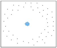
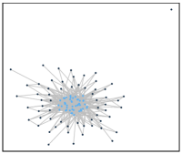
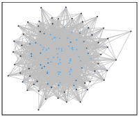
Figure 1: Graphs of Chung-Lu type generated with Algorithm 3 on $\Omega=[0,1]$ with $n=1000$, $m=\lceil\sqrt{\epsilon n}\rceil$ and $a=b=100$. Graph 1 shows a realization of the “true” graph with $\mathcal{X}=\{0,\ldots,0,1,\ldots,1\}$. Graph 2-4 are realizations of the private synthetic graph generated with Laplacian noise $\text{Lap}_{\mathbb{Z}}(1/\epsilon)$ for $\epsilon\in\{1,0.1,0.01\}$. The vertex color visualizes the attribute, where small attributes correspond to dark colors.

4 Theoretical guarantees on utility

In this section we give theoretical results for the PSGG algorithm which show conditions under which the differentially private synthetic network distribution is close to the distribution of the “true” graph. Algorithm 3. In particular, we study the differences between the “true” graph $(\mathrm{H},\mathrm{T})$ that was constructed using the true data $\mathcal{X}$, and the private synthetic graph $(\Xi,\Sigma)$ that was constructed using the private synthetic measure $\hat{\nu}$. In the first part we consider the accuracy of Algorithm 3 while the second part analyzes the difference in distribution. All proofs details are deferred to App. C.

4.1 Accuracy of Algorithm 3

In the following result we control the accuracy measure, i.e. we bound the expected distance between the true attributed random graph $(\mathrm{H},\mathrm{T})$ and the private synthetic attributed random graph $(\Xi,\Sigma)$ constructed by Algorithm 3 with respect to the FGW distance, see Section 2.2. That is, we study $\mathbb{E}(d_{FGW}(\eta^{(\mathrm{H},\mathrm{T})},\eta^{(\Xi,\Sigma)}))$, where $\eta^{(\mathrm{H},\mathrm{T})}$ and $\eta^{(\Xi,\Sigma)}$ are random measures that capture the (attributed) graph information of $(\mathrm{H},\mathrm{T})$ and $(\Xi,\Sigma)$, respectively. We recall the notion of diameter; $diam(\Omega)=\sup_{x,y\in\Omega}d(x,y).$

Theorem 4.1.

Let $(\mathrm{H},\mathrm{T})$ and $(\Xi,\Sigma)$ be the “true” and private synthetic random graphs of expected size $a>0$ and $b>0$, respectively, constructed by Algorithm 3. Then

$$\mathbb{E}\big{(}d_{FGW}(\eta^{(\mathrm{H},\mathrm{T})},\eta^{(\Xi,\Sigma)})\big{)} \leq\tilde{C}_{1}\,\max_{k\in[m]}\mathrm{diam}(\Omega_{k})\frac{1}{1+\frac{a\wedge b}{|a-b|}1\hskip-3.87495pt1_{\{|a-b|>0\}}}+4\tilde{C}_{2}\frac{m}{n}\mathbb{E}(|\Lambda|)$$

$$+\tilde{C}_{2}\bigg{(}1-\frac{1}{\big{(}1+\frac{a\wedge b}{|a-b|}\big{)}^{2}}\bigg{)}1\hskip-3.87495pt1_{\{|a-b|>0\}},$$

where $\tilde{C}_{1}=1-\alpha+\alpha(2\,C\,L_{\kappa})$ and $\tilde{C}_{2}=(1-\alpha)\mathrm{diam}(\Omega)+\alpha\min\{C,2\,C\,L_{\kappa}\mathrm{diam}(\Omega)\}$ with $\alpha\in[0,1]$ and $C>0$ parameters of the FGW metric and $L_{\kappa}$ the Lipschitz constant of edge connection function $\kappa$.

In what follows we sketch the idea of the proof and refer to App. C for details. Note that the construction of the graphs in Algorithm 3 allows us to significantly reduce the costs of the estimates.
Sketch of the proof of Theorem 4.1: For two pairs of vertices $(X_{i},Y_{j})$ we can bound the attribute cost by $\mathrm{diam}(\Omega)$ and the edge cost by $\min\{C,2\,C\,L_{\kappa}\mathrm{diam}(\Omega)\}$ using the Lipschitz property of $\kappa$ for the second term. Under the assumption that $(X_{i},Y_{j})$ are in the same cell, this bound can be improved to $\max_{k\in[m]}\mathrm{diam}(\Omega_{k})$ for the vertex part and $2\,C\,L_{\kappa}\max_{k\in[m]}\mathrm{diam}(\Omega_{k})$ for the edge part; details are found in Appendix C. We then obtain the result by conditioning on the (minimal) number $Z$ of vertices $(X_{i},Y_{i})$ that are in a common cell.

We consider a special case of Theorem 4.1 to give a more thorough discussion of the obtained bound. We restrict to discrete Laplacian noise $\Lambda\sim\text{Lap}_{\mathbb{Z}}(1/\epsilon)$ which yields $\mathbb{E}|\Lambda|=2\frac{e^{-\epsilon}}{1-e^{-2\epsilon}}$, see Inusah and Kozubowski (2006), and set $\Omega=[0,1]^{d}$ to be the $d$-dimensional unit cube. Moreover, we let $a=b$ and choose the sample size $m=\lceil f_{n}(\epsilon)n\rceil$ for a function $f_{n}:\mathbb{R}_{+}\to\mathbb{R}_{+}$. Under these assumptions the bound obtained above simplifies to the following result.

Corollary 4.2.

Let $m=\lceil f_{n}(\epsilon)n\rceil$ and consider graphs generated by Algorithm 3 using discrete Laplacian noise and a partition $(\Omega_{k})_{k=1}^{m}$ which satisfies $\mathrm{diam}(\Omega_{k})\asymp m^{-1/d}$. Assume that the graphs have the same expected size $a=b$ with attributes in $\Omega=[0,1]^{d}$. Then Theorem 4.1 simplifies to

$$\mathbb{E}\big{(}d_{FGW}(\eta^{(\mathrm{H},\mathrm{T})},\eta^{(\Xi,\Sigma)})\big{)} \leq\tilde{C}_{1}m^{-1/d}+4\tilde{C}_{2}f_{n}(\epsilon)\frac{e^{-\epsilon}}{1-e^{-2\epsilon}}.$$ (3)

A reasonable choice of the function $f_{n}$ is essential to obtain good convergence rates and we refer to Section 4.3 for an analysis.

Remark 4.3.

A special case of Theorem 4.1 can be obtained by setting the edge probability function $\kappa\equiv 0$. Then we a.s. have no edges and the random graphs constructed as in Algorithm 3 can be described by their vertex processes $\mathrm{H}$ and $\Xi$. The FGW distance then simplifies to the 1-Wasserstein distance. In particular, we can bound the accuracy of Algorithm 3 for vertex generation with the results obtained in Theorem 4.1 by setting $\alpha=0$.

4.2 Bounds on the difference between the graph distributions

In the following we analyze and measure the differences between the distribution $(P^{\mu^{a}_{\mathcal{X}}}\otimes Q^{\kappa})$ of the “true” random graph $(\mathrm{H},\mathrm{T})$ and the distribution $(P^{\mu^{b}_{\mathcal{Y}}}\otimes Q^{\kappa})$ of the private synthetic random graph $(\Xi,\Sigma)$. To measure the distance of random graph distributions, we consider the Wasserstein distance with respect to the FGW distance as an underlying metric. More precisely, we define

$$d_{\mathcal{F}}(P^{\mu^{b}_{\mathcal{Y}}}\otimes Q^{\kappa},P^{\mu^{a}_{\mathcal{X}}}\otimes Q^{\kappa})=\sup\limits_{f\in\mathcal{F}}\big{|}\mathbb{E}(f(\Xi,\Sigma))-\mathbb{E}(f(\mathrm{H},\mathrm{T}))\big{|},$$ (4)

where $\mathcal{F}$ is the set of test functions $f:\mathbb{G}\to\mathbb{R}$ that are Lipschitz with respect to the FGW distance, see Section 2.2. As a direct consequence of this Lipschitz property and Theorem 3.1, the results obtained in Section 4.1 can be in particular used to bound the above distance.

We derive upper bounds for these distances of random graph distributions by adapting general bounds from Schuhmacher and Wirth (2024). We remark that, in general, it is possible to consider different classes of test functions and thus obtain different types of so called integral probability metrics. Our approach will then work analogously, however, the obtained upper bounds and rates will strongly depend on the choice of test functions.

Theorem 4.4.

Let $(P^{\mu^{a}_{\mathcal{X}}}\otimes Q^{\kappa})$ and $(P^{\mu^{b}_{\mathcal{Y}}}\otimes Q^{\kappa})$ be distributions of the “true” and the private synthetic random graph of expected size $a>0$ and $b>0$, respectively, constructed as in Section 3.1 by using a probability measure $\hat{\nu}$ created by Algorithm 1 with random noise $\Lambda$. Then

$$d_{\mathcal{F}}(P^{\mu^{b}_{\mathcal{Y}}}\otimes Q^{\kappa},P^{\mu^{a}_{\mathcal{X}}}\otimes Q^{\kappa})$$

$$\leq\bigg{(}1+\frac{1}{1+\frac{b}{c}1\hskip-3.87495pt1_{\{c>0\}}}\bigg{)}(1-\alpha)\,\max_{k\in[m]}\mathrm{diam}(\Omega_{k})+\tilde{C}_{2}\bigg{(}1-\frac{1}{\big{(}1+\frac{b}{c}\big{)}^{2}}\bigg{)}1\hskip-3.87495pt1_{\{c>0\}}$$

$$+2c_{V}(a\wedge b)\frac{a\wedge b}{n}\mathrm{Leb}^{d}(\Omega)\mathbb{E}|\Lambda|+c_{E}(a\wedge b)\,2L_{\kappa}\max_{k\in[m]}\mathrm{diam}(\Omega_{k})^{3}(a\wedge b)^{2},$$

where

$$c_{V}(c) :=\min\biggl{\{}C_{\alpha},\frac{1}{c}\,\bigl{(}1+({1-e^{-{c}}})\log^{+}{c}\bigr{)}\,C_{\alpha}\biggr{\}},$$

$$c_{E}(c) :=\min\biggl{\{}1,\frac{2-e^{-c}}{c}-\frac{1}{c^{2}}\Bigl{(}\frac{3}{2}-e^{-c}\Bigr{)}\biggr{\}}\;\alpha C$$

for $C_{\alpha}:=(1-\alpha)\mathrm{diam}(\Omega)+\alpha C$ and $\tilde{C}_{2}=(1-\alpha)\mathrm{diam}(\Omega)+\alpha\min\{C,2CL_{\kappa}\mathrm{diam}(\Omega)\}$ with $\alpha\in[0,1]$ and $C>0$ parameters of the FGW distance and $L_{\kappa}$ the Lipschitz constant of the edge connection function $\kappa$.

In what follows, we give a short sketch of the proof for Theorem 4.4; we refer to App C for details.

Sketch of the proof of Theorem 4.4. The proof is based on results of (Schuhmacher and Wirth, 2024, Theorem 4.7), which provides upper bounds on the distance of two random (attributed) graph distributions, derived by Stein’s method. The bounds in (Schuhmacher and Wirth, 2024, Theorem 4.7) are of total variation type and thus will not vanish in a direct comparison (as the attribute measures have different support). Furthermore, the bound is sensitive to the number of vertices. More precisely, the “true” graph has mass $N$ while the private synthetic graph has mass $M$. We approach this issue by creating intermediate graphs that are supported on whole $\Omega$ and have the same size $N\wedge M$. These intermediate graphs are constructed by resampling the attributes of the first $N\wedge M$ points in each cell while keeping the edge probabilities of the original graph. The difference between the original graphs and their corresponding intermediate graphs can be analyzed using a coupling. It remains to compare the intermediate graphs. This now can be done by an application of Schuhmacher and Wirth (2024, Theorem 4.7), stated in terms of their so-called GOSPA metric. Under a suitable choice of parameters in the GOSPA metric, the FGW distance is a lower bound for the GOSPA metric, which suffices for our purposes. Finally, we assemble all results to obtain to obtain the claimed upper bound.

Corollary 4.5.

Consider graphs being distributed according to Section 3.1 w.r.t. a probability measure $\hat{\nu}$ created by Algorithm 1 using discrete Laplacian noise and a partition $(\Omega_{k})_{k=1}^{m}$ satisfying $\mathrm{diam}(\Omega_{k})\asymp m^{-1/d}$. Furthermore, set $a=b$ and $\Omega=[0,1]^{d}$. Then Theorem 4.4 simplifies to

$$d_{\mathcal{F}}(P^{\mu^{b}_{\mathcal{Y}}}\otimes Q^{\kappa},P^{\mu^{a}_{\mathcal{X}}}\otimes Q^{\kappa})\leq 2(1-\alpha)\,m^{-1/d}+\frac{2\bigl{(}1+\log^{+}{a}\bigr{)}}{\epsilon n}C_{\alpha}\epsilon\frac{e^{-\epsilon}}{1-e^{-2\epsilon}}+4\alpha CL_{\kappa}m^{-3/d}a.$$ (5)

Similar to the results in Section 4.1, a reasonable choice of the (expected) size $a=a_{n}$ of the random graph and the partition size $m=\lceil f_{n}(\epsilon)n\rceil$ are essential to obtain good convergence rates, as we discuss in the next section.

4.3 Choice of parameters

In practice, we often are given a dataset $\mathcal{X}$ of size $n$ and a privacy level $\epsilon$ and have to make suitable choices for the expected size of the graphs $a$ and the partition size $m=\lceil f_{n}(\epsilon)n\rceil$. Here we discuss a suitable choice of these parameters using the rates obtained by Theorem 4.1 and Theorem 4.4. Again, we restrict to graphs having the same expected size $a=b$ with attributes on the unit cube $\Omega=[0,1]^{d}$ and assume that the graphs are generated by Algorithm 3 using discrete Laplacian noise $\Lambda\sim\text{Lap}_{\mathbb{Z}}(1/\epsilon)$. Furthermore, we let $m=\lceil f_{n}(\epsilon)n\rceil$ for some function $f_{n}$ and remark that for any $\epsilon\geq 0$

$$\epsilon\,\frac{e^{-\epsilon}}{{1-e^{-2\epsilon}}}\leq 1/2.$$

Then Corollary 4.2 yields

$$d_{\mathcal{F}}(P^{\mu^{b}_{\mathcal{Y}}}\otimes Q^{\kappa},P^{\mu^{a}_{\mathcal{X}}}\otimes Q^{\kappa})\leq\mathbb{E}\big{(}d_{FGW}(\eta^{(\mathrm{H},\mathrm{T})},\eta^{(\Xi,\Sigma)})\big{)}\leq\tilde{C}_{1}(f_{n}(\epsilon)n)^{-1/d}+2\tilde{C}_{2}\frac{f_{n}(\epsilon)}{\epsilon},$$ (6)

where the first inequality follows from the definition of $d_{\mathcal{F}}$, see Section 4.2; while Corollary 4.5 states

$$d_{\mathcal{F}}(P^{\mu^{b}_{\mathcal{Y}}}\otimes Q^{\kappa},P^{\mu^{a}_{\mathcal{X}}}\otimes Q^{\kappa})$$ (7)

$$\leq 2(1-\alpha)\,m^{-1/d}+\frac{2\bigl{(}1+\log^{+}{a}\bigr{)}}{\epsilon n}C_{\alpha}\epsilon\frac{e^{-\epsilon}}{1-e^{-2\epsilon}}+4\alpha CL_{\kappa}m^{-3/d}a.$$

The speed of convergence depends on the choice of $f_{n}$ as well as the expected size of the graphs $a$. We start with a suitable choice of graph size. Consider the bound in (7). On the one hand, we would like to choose the expected graph size $a=a_{n}$ as large as possible to have a good sample size for our graphs. On the other hand, (5) yields better bounds the smaller $a$ is. As the first term in (5) does not depend on $a$, an optimal choice of $a$ is such that the first and third terms in (5) have the same speed of convergence. Note that we do not consider the second term here as due to the log-term the influence of $a$ is negligible compared to the third term. Then

$$m^{-1/d}\asymp am^{-3/d}\iff a=m^{2/d}.$$

In particular, using that $m=\lceil f_{n}(\epsilon)n\rceil$ Inequality (7) turns to

$$d_{\mathcal{F}}(P^{\mu^{b}_{\mathcal{Y}}}\otimes Q^{\kappa},P^{\mu^{a}_{\mathcal{X}}}\otimes Q^{\kappa})\leq\big{(}\!2(1-\alpha)+4\alpha CL_{\kappa}\!\big{)}(f_{n}(\epsilon)n)^{-\frac{1}{d}}+C_{\alpha}(1\!+2\log^{+}\!(f_{n}(\epsilon)n)\!)(\epsilon n)^{-1}.$$ (8)

It remains to find a suitable choice of $m=\lceil f_{n}(\epsilon)n\rceil$ by deriving an optimal decay of $f_{n}(\epsilon)$ as $\epsilon\to 0$. Note that in both, (6) and (8), we obtain a trade-off for the choice of $f_{n}$. More precisely, to obtain fast convergence (to zero) in the first terms, we would like $f_{n}(\epsilon)$ to go to zero slowly. On the other hand, the second terms decrease faster the faster $f_{n}(\epsilon)$ goes to zero. However, note that due to the logarithmic expression the observed trade-off in (8) is weaker than the trade-off in (6). In particular, we focus on (6) and derive an optimal decay for $f_{n}$ as follows.

Due to the trade-off between the two terms in (6), an optimal decay for $f_{n}$ can be obtained by assuming the same speed of convergence for both terms in (6). This corresponds to setting

$$\frac{f_{n}(\epsilon)}{\epsilon}\asymp\big{(}f_{n}(\epsilon)n\big{)}^{-1/d}\iff f_{n}(\epsilon)\asymp\epsilon^{\frac{d}{d+1}}\,n^{-\frac{1}{d+1}}.$$

In particular, under the above assumptions (6) and thus Corollary 4.2 simplify to

$$d_{\mathcal{F}}(P^{\mu^{b}_{\mathcal{Y}}}\otimes Q^{\kappa},P^{\mu^{a}_{\mathcal{X}}}\otimes Q^{\kappa})\leq\mathbb{E}\big{(}d_{FGW}(\eta^{(\mathrm{H},\mathrm{T})},\eta^{(\Xi,\Sigma)})\big{)} \leq(\tilde{C}_{1}+2\tilde{C}_{2})\big{(}\epsilon\,n\big{)}^{-\frac{1}{d+1}}.$$

Similarly, (8) and thus Corollary 4.5 turn to

$$d_{\mathcal{F}}(P^{\mu^{b}_{\mathcal{Y}}}\otimes Q^{\kappa},P^{\mu^{a}_{\mathcal{X}}}\otimes Q^{\kappa})\leq\big{(}2(1-\alpha)+4\alpha CL_{\kappa}\big{)}(\epsilon n)^{-\frac{1}{d+1}}+C_{\alpha}\bigg{(}1+\frac{2}{d+1}\log^{+}(\epsilon n)\bigg{)}(\epsilon n)^{-1}.$$

In particular, with the above choice of $f_{n}$ and $a$ we obtain the same speed of convergence for both approaches. Note however, that we optimized $f_{n}$ w.r.t. the results obtained in Section 4.1. Hence, for a different choice of $f_{n}$ the results stated in Section 4.2 can yield improved rates.

We end this Section by giving a table with precise upper bounds, Table 1 and refer to Appendix C for explicit upper bounds in different parameter settings. There is no uniformly better bound Corollary 4.2 gives smaller bounds than Corollary 4.5 when $\epsilon$ is large. Both bounds decrease when $n$ increases.

		$n$
		100		1000		10.000
		Cor 4.2	Cor 4.5	Cor 4.2	Cor 4.5	Cor 4.2	Cor 4.5
	1	0.751	0.681	0.349	0.304	0.162	0.14
$\epsilon$	0.1	1.599	1.602	0.751	0.681	0.349	0.304
	0.01	3.061	3.721	1.599	1.602	0.751	0.681

Table 1: Explicit bounds obtained in Corollary 4.2 and Corollary 4.5 assuming discrete Laplacian noise and $\Omega=[0,1]^{2}$, $\alpha=1/2$ as well as $C=L_{\kappa}=1$. Furthermore, $m=\lceil f_{n}(\epsilon)n\rceil$ with $f_{n}$ optimal and $a$ optimal w.r.t. Section 4.3.

5 Conclusion and Future Works

In this work, we proposed an algorithm that jointly generates a network representation and a private synthetic network from a given dataset. We provided a theoretical analysis of our algorithm studying the accuracy w.r.t. the fused Gromov Wasserstein distance and comparing the corresponding network distributions. Under additional assumptions, we derived optimal parameter choices and deduced that in this case our bounds are $\mathcal{O}(n^{-1/(d+1)})$.

An interesting further direction would be the consideration of directed networks. Furthermore, it would be worthwhile to study networks with weighted edges. Here challenges lie in a possible dependence of the weight on the existence of an edge. Moreover, it would require a new notion of accuracy for attributed networks with weighted edges.

It would be interesting to combine the node privacy studied in this paper with a suitable notion of edge privacy. This could be achieved, for example, by adapting the rule how edges are being created by including a resampling mechanism on the edges. However, a suitable notion of such a joint privacy measure to our knowledge has not yet been investigated.

Finally, we intend to extend our results to include $(\epsilon,\delta)$- differential privacy, see Dwork (2006), thus allowing for more discrete noise distributions, e.g., a discrete Gaussian distribution (Canonne et al., 2020).

Appendix A More Related Works

This section details related works about differential privacy in graphs.

Differential Privacy in Graphs: Vertex and edge differential privacy in graphs were introduced in [Kasiviswanathan et al., 2013] using the rewiring distance. Several works focus on differentially private graph publishing [Jian et al., 2021, Day et al., 2016, Hou et al., 2023]. Other works propose practical approaches for private synthetic graph generation under different notions of privacy [Qin et al., 2017, Zahirnia et al., 2024]. In contrast to these approaches, our work provides a theoretical foundation for private synthetic graph generation, with rigorous guarantees.

Appendix B Proofs and details of Section 2

Proof.

Let $\nu$ be a discrete signed probability measure on $\mathcal{Y}$. Then for any probability measure $\tau$ on $\mathcal{Y}$ the total variation distance between $\nu$ and $\tau$ is given by

$$d_{TV}(\nu,\tau)=\sum_{i=1}^{m}|\nu_{i}-\tau_{i}|,$$

where $\nu_{i}:=\nu(\{y_{i}\})$ and $\tau_{i}:=\tau(\{y_{i}\})$, see Section 2.3. Thus, finding the closest probability measure with respect to the total variation distance is equivalent to solving the program (P$1$) given by

$$\min\quad \sum_{i=1}^{m}|\nu_{i}-\tau_{i}| 1$$ (P)

s.t. $$\sum_{i=1}^{m}\tau_{i}=1,\quad\tau_{i}\geq 0,\quad\forall i\leq m.$$

Then as $|\nu_{i}-\tau_{i}|=\max\{\nu_{i}-\tau_{i},\tau_{i}-\nu_{i}\}$, minimizing the absolute value $|\nu_{i}-\tau_{i}|$ is equivalent to finding the minimal $u_{i}\geq\max\{\nu_{i}-\tau_{i},\tau_{i}-\nu_{i}\}$. In particular, (P$1$) is equivalent to solving the linear program in Algorithm 2. ∎

Appendix C Proofs and details of Section 4

Proof.

We show that the two attributed random graphs constructed in Algorithm 3 define a coupling of the graph models introduced in Section 3.1. We write $\mathbb{P}_{\lambda}$ and $\mathbb{E}_{\lambda}$ to denote the conditional probability and expectation given $\lambda=(\lambda_{i})_{i=1}^{m}$. Recall that the probability measure $\hat{\nu}$ depends on $\lambda$. We write $(\mathrm{H},\mathrm{T})$ and $(\Xi,\Sigma)$ for the graphs constructed according to the graph model in Section 3.1 and $(\hat{\mathrm{H}},\hat{\mathrm{T}})$ as well as $(\hat{\Xi},\hat{\Sigma})$ for the graphs constructed in Algorithm 3.

Step 1: Coupling of the vertex process
Consider the total number of vertices $N\sim\text{Poi}(a)$ and $M\sim\text{Poi}(b)$ and assume without loss of generality that $a\geq b$. Then $N\overset{d}{=}M+K_{N}$ for $K_{N}\sim\text{Poi}(a-b)$. In particular, this defines a coupling of $N$ and $M$ such that $N\geq M$.

For $k\in[m]$, let $N_{k}:=\mathrm{H}(\Omega_{k})$ be the number of points $(X_{i},U_{i})$ of $\mathrm{H}$ whose attributes $X_{i}$ are in $\Omega_{k}$. As the $X_{i}$ were chosen uniformly from $\mathcal{X}$ we obtain

$$\mathbb{P}(X_{i}\in\Omega_{k})=\frac{\#\{x_{j}\in\Omega_{k}:j\in[n]\}}{n}=\frac{n_{k}}{n}.$$

Given the total number of points $N$ in $\eta$, the vector $\mathbb{N}:=(N_{1},\ldots,N_{m})$ of attribute counts in the partition sets $(\Omega_{i})_{i\in[m]}$ has a multinomial distribution, $\mathbb{N}\,|\,N\sim\text{Multin}(N,(\frac{n_{1}}{n},\ldots,\frac{n_{m}}{n})).$ Analogously, for $k\in[m]$ let $M_{k}:=\Xi(\Omega_{k})$ be the number of points $(Y_{i},V_{i})$ of $\Xi$ whose attributes $Y_{i}$ are in $\Omega_{k}$. Then we have

$$\mathbb{P}_{\lambda}(Y_{i}\in\Omega_{k})=\mathbb{P}(Y_{i}=y_{k})=\hat{\nu}_{k}$$

and, given the total number of points $M$ in $\Xi$, we obtain that the conditional distribution is $\mathbb{M}\,|\,M:=(M_{1},\ldots,M_{m})\,|\,M\sim\text{Multin}(M,(\hat{\nu}_{1},\ldots,\hat{\nu}_{m}))$.

We show that the vertex counts constructed in Algorithm 3 obtain the same distribution. Let $\mathbb{Z}^{j}:=(Z^{j}_{1},\ldots,Z^{j}_{m})\in\{0,1\}^{m}$, $j\in[M]$, be independent random variables defined by

$$\mathbb{P}_{\lambda}(\mathbb{Z}^{j}=(l_{1},\ldots,l_{m})) =\prod_{k\in[m]}\bigg{(}\frac{n_{k}}{n}\wedge\hat{\nu}_{k}\bigg{)}^{l_{k}},\quad\mbox{ for }l_{1},\ldots,l_{m}\in\{0,1\}\mbox{ such that }\sum_{k\in[m]}l_{k}=1;$$

$$\mathbb{P}_{\lambda}(\mathbb{Z}^{j}=(0,\ldots,0)) =1-\sum_{\begin{subarray}{c}l_{1},\ldots,l_{m}\in\{0,1\}\\ \sum_{k\in[m]}l_{k}=1\end{subarray}}\mathbb{P}_{\lambda}(\mathbb{Z}^{j}=(l_{1},\ldots,l_{m}))=1-\sum_{k\in[m]}\frac{n_{k}}{n}\wedge\hat{\nu}_{k}.$$

Note that this construction corresponds to the choice of common vertex counts in Algorithm 3.

We describe the construction of non-common vertex counts. First, define $\mathbb{K}\,|\,(N-M):=(K_{1},\cdots,K_{m})\,|\,(N-M)\sim\text{Multin}(N-M,(\frac{n_{1}}{n},\ldots,\frac{n_{m}}{n}))$.

If $\frac{n_{k}}{n}=\hat{\nu}_{k}$ for all $k\in[m]$, then $\mathbb{N}\overset{d}{=}\mathbb{M}+\mathbb{K}$ and we obtain a coupling $\mathbb{N}$ and $\mathbb{M}$ such that $N_{k}=M_{k}+K_{k}=\sum_{j\in[M]}Z_{k}^{j}+K_{k}$ for all $k\in[m]$.

Otherwise, there exists a $k\in[m]$ such that $\frac{n_{k}}{n}\neq\hat{\nu}_{k}$ and we obtain $\mathbb{P}_{\lambda}(\mathbb{Z}^{j}=(0,\ldots,0))>0$. For $j\in[M]$ we then define $\mathbb{Z}^{N,j}:=(Z_{1}^{N,j},\ldots,Z_{m}^{N,j})$ by

$$\mathbb{P}_{\lambda}(\mathbb{Z}^{N,j}=(l_{1},\ldots,l_{m}))=\big{(}\mathbb{P}_{\lambda}(\mathbb{N}^{j}=(l_{1},\ldots,l_{m}))-\mathbb{P}_{\lambda}(\mathbb{Z}^{j}=(l_{1},\ldots,l_{m}))\big{)}\mathbb{P}_{\lambda}(\mathbb{Z}^{j}=(0,\ldots,0))^{-1},$$

where $\mathbb{N}^{j}\sim\text{Multin}(1,(\frac{n_{1}}{n},\ldots,\frac{n_{m}}{n}))$ and $l_{1},\ldots,l_{m}\in\{0,1\}$ such that $\sum_{k\in[m]}l_{k}=1$. Note that this defines a probability distribution as

$$\sum_{\begin{subarray}{c}l_{1},\ldots,l_{m}\in\{0,1\}\\ \sum_{k\in[m]}l_{k}=1\end{subarray}}\mathbb{P}_{\lambda}(\mathbb{Z}^{N,j}=(l_{1},\ldots,l_{m}))$$

$$=\bigg{(}1-\sum_{\begin{subarray}{c}l_{1},\ldots,l_{m}\in\{0,1\}\\ \sum_{k\in[m]}l_{k}=1\end{subarray}}\mathbb{P}_{\lambda}(\mathbb{Z}^{j}=(l_{1},\ldots,l_{m}))\bigg{)}\mathbb{P}_{\lambda}(\mathbb{Z}^{j}=(0,\ldots,0))^{-1}=1.$$

Furthermore, $\mathbb{Z}^{N,j}=(l_{1},\ldots,l_{m})\,|\,(\mathbb{Z}^{j}=(0,\ldots,0))\sim\text{Multin}(1,(\frac{n_{1}}{n},\ldots,\frac{n_{m}}{n}))$ and thus $(Z_{1}^{N,j}+K_{1},\ldots,Z_{m}^{N,j}+K_{m})\sim\text{Multin}(N-Z,(\frac{n_{1}}{n},\ldots,\frac{n_{m}}{n}))$ for $Z=\sum_{j\in[M]}\sum_{k\in[m]}Z_{k}^{j}$. In particular, the construction of $\mathbb{Z}^{N,j}$ and $\mathbb{K}$ corresponds to the creation of non-common vertex counts in Algorithm 3. Analogously we define $\mathbb{Z}^{M,j}$ and set $\hat{\mathbb{N}}=\sum_{j\in[M]}\hat{\mathbb{N}}^{j}+\sum_{j\in[N]\setminus[M]}{\mathbb{N}}^{j}=\sum_{j\in[M]}\mathbb{Z}^{j}+\mathbb{Z}^{N,j}1\hskip-3.87495pt1_{\{\mathbb{Z}^{j}=(0,\ldots,0)\}}+\mathbb{L}$ as well as $\hat{\mathbb{M}}=\sum_{j\in[M]}\hat{\mathbb{M}}^{j}=\sum_{j\in[M]}\mathbb{Z}^{j}+\mathbb{Z}^{M,j}1\hskip-3.87495pt1_{\{\mathbb{Z}^{j}=(0,\ldots,0)\}}$. Then $(\hat{\mathbb{N}},\hat{\mathbb{M}})$ is a coupling of $\mathbb{N}$ and ${\mathbb{M}}$ as for any $j\in[M]$

$$\mathbb{P}_{\lambda}(\hat{\mathbb{N}}^{j}=(l_{1},\ldots,l_{m}))$$

$$=\mathbb{P}_{\lambda}(\hat{\mathbb{N}}^{j}=(l_{1},\ldots,l_{m}),\mathbb{Z}^{j}=(0,\ldots,0))+\mathbb{P}_{\lambda}(\hat{\mathbb{N}}^{j}=(l_{1},\ldots,l_{m}),\mathbb{Z}^{j}\neq(0,\ldots,0))$$

$$=\mathbb{P}_{\lambda}(\mathbb{Z}^{N,j}=(l_{1},\ldots,l_{m}))\mathbb{P}_{\lambda}(\mathbb{Z}^{j}=(0,\ldots,0))+\mathbb{P}_{\lambda}({\mathbb{Z}^{j}}=(l_{1},\ldots,l_{m}))$$

$$=\mathbb{P}_{\lambda}({\mathbb{N}}^{j}=(l_{1},\ldots,l_{m}))$$

and analogously $\mathbb{P}_{\lambda}(\hat{\mathbb{M}}^{j}=(l_{1},\ldots,l_{m}))=\mathbb{P}_{\lambda}({\mathbb{M}}^{j}=(l_{1},\ldots,l_{m}))$. Furthermore, by the construction of $\mathbb{Z}$ we obtain for any $j\in[M]$ that

$$\mathbb{P}_{\lambda}(\hat{\mathbb{N}}^{j}\neq\hat{\mathbb{M}}^{j})=\mathbb{P}_{\lambda}(\mathbb{Z}^{j}=(0,\ldots,0)).$$

We now use the fact that the vertex counts in Algorithm 3 have the correct marginal distributions to follow that the vertex processes $\hat{\mathrm{H}}$ and $\hat{\Xi}$ have the correct marginal distributions. Recall that we constructed $\hat{\mathrm{H}}=\sum_{i=1}^{m}\sum_{j=1}^{\hat{N_{i}}}\delta_{(X_{ij},U_{ij})}$ for $X_{ij}\sim\mathcal{U}(\mathcal{X}\cap\Omega_{i})$, $U_{ij}\sim\mathcal{U}([0,1])$ and $\hat{\Xi}=\sum_{i=1}^{m}\sum_{j=1}^{\hat{M_{i}}}\delta_{(Y_{ij},U_{ij})}$ for $Y_{ij}=y_{i}$. Note that the distributions of the attributes, the identifiers, and the number of attributes in each partition set are unchanged compared to the graph model in Section 3.1. Hence, this defines a coupling $(\hat{\mathrm{H}},\hat{\Xi})$ of the vertex processes $\mathrm{H}$ and $\Xi$.

Step 2: Coupling of the edge process
Based on the coupling of the vertex processes we can now show that the edge processes $(\hat{\mathrm{T}},\hat{\Sigma})$ constructed in Algorithm 3 define a coupling of the edge processes $\mathrm{T}$ and $\Sigma$. Recall that the existence of an edge $(U_{ij},U_{i^{\prime}j^{\prime}})$ in $\mathrm{T}$ and $\Sigma$ is determined by Bernoulli random variables $K_{ij}^{\mathrm{T}}$ and $K_{ij}^{\Sigma}$, respectively, see Section 3.1. Furthermore, the connection probabilities in Algorithm 3 were defined by

$$\mathbb{P}_{\lambda}((\hat{K}^{\mathrm{T}}_{iji^{\prime}j^{\prime}},\hat{K}^{\Sigma}_{iji^{\prime}j^{\prime}})=(1,1)) =\kappa(X_{ij},X_{i^{\prime}j^{\prime}})\wedge\kappa(Y_{ij},Y_{i^{\prime}j^{\prime}})$$

$$\mathbb{P}_{\lambda}((\hat{K}^{\mathrm{T}}_{iji^{\prime}j^{\prime}},\hat{K}^{\Sigma}_{iji^{\prime}j^{\prime}})=(1,0)) =\kappa(X_{ij},X_{i^{\prime}j^{\prime}})-(\kappa(X_{ij},X_{i^{\prime}j^{\prime}})\wedge\kappa(Y_{ij},Y_{i^{\prime}j^{\prime}}))$$

$$\mathbb{P}_{\lambda}((\hat{K}^{\mathrm{T}}_{iji^{\prime}j^{\prime}},\hat{K}^{\Sigma}_{iji^{\prime}j^{\prime}})=(0,1)) =\kappa(Y_{ij},Y_{i^{\prime}j^{\prime}})-(\kappa(X_{ij},X_{i^{\prime}j^{\prime}})\wedge\kappa(Y_{ij},Y_{i^{\prime}j^{\prime}}))$$

$$\mathbb{P}_{\lambda}((\hat{K}^{\mathrm{T}}_{iji^{\prime}j^{\prime}},\hat{K}^{\Sigma}_{iji^{\prime}j^{\prime}})=(0,0)) =1-\kappa(X_{ij},X_{i^{\prime}j^{\prime}})\vee\kappa(Y_{ij},Y_{i^{\prime}j^{\prime}})$$

for any $i,i^{\prime}\in[m]$ and any $j\in[Z_{i}]$ and $j^{\prime}\in[Z_{i^{\prime}}]$ and by $\hat{K}^{\mathrm{T}}_{iji^{\prime}j^{\prime}}\sim\text{Ber}(\kappa(X_{ij},X_{i^{\prime}j^{\prime}}))$ and $\hat{K}^{\Sigma}_{iji^{\prime}j^{\prime}}\sim\text{Ber}(\kappa(Y_{ij},Y_{i^{\prime}j^{\prime}}))$ for any $(j,j^{\prime})$ such that $j>Z_{i}$ or $j^{\prime}>Z_{j^{\prime}}$. Clearly, this construction of $\hat{K}^{\mathrm{T}}$ and $\hat{K}^{\Sigma}$ corresponds to a maximal coupling of the two Bernoulli random variables $K_{ij}^{\mathrm{T}}$ and $K_{ij}^{\Sigma}$. In particular,

$$\mathbb{P}_{\lambda}(\hat{K}^{\mathrm{T}}_{iji^{\prime}j^{\prime}}\neq\hat{K}^{\Sigma}_{iji^{\prime}j^{\prime}})=|\kappa(X_{ij},X_{i^{\prime}j^{\prime}})-\kappa(Y_{ij},Y_{i^{\prime}j^{\prime}})|.$$

Thus, setting

$$\hat{\mathrm{T}}=\sum_{i,i^{\prime}=1}^{m}\sum_{j=1}^{\hat{N}_{i}}\sum_{j^{\prime}=1}^{\hat{N}_{i^{\prime}}}\hat{K}^{\mathrm{T}}_{iji^{\prime}j^{\prime}}\delta_{\{U_{ij},U_{i^{\prime}j^{\prime}}\}}\mbox{ and }\hat{\Sigma}=\sum_{i,i^{\prime}=1}^{m}\sum_{j=1}^{\hat{M}_{i}}\sum_{j^{\prime}=1}^{\hat{M}_{i^{\prime}}}\hat{K}^{\Sigma}_{iji^{\prime}j^{\prime}}\delta_{\{U_{ij},U_{i^{\prime}j^{\prime}}\}}$$

yields a coupling of the edge processes. Overall, this shows that $(\hat{\mathrm{H}},\hat{\mathrm{T}})$ and $(\hat{\Xi},\hat{\Sigma})$ constructed in Algorithm 3 yield a coupling of $({\mathrm{H}},{\mathrm{T}})$ and $({\Xi},{\Sigma})$ constructed in Section3.1 and thus have the claimed (marginal) distributions. ∎

Proof.

We write $\mathbb{P}_{\lambda}$ and $\mathbb{E}_{\lambda}$ to denote the conditional probability and expectation given $\lambda=(\lambda_{i})_{i=1}^{m}$ and assume w.l.o.g. that $a\geq b$. We stick to the notation introduced in the Proof of Theorem 3.1, see App. C. In particular, we denote the graphs constructed with Algorithm 3 by $(\hat{\mathrm{H}},\hat{\mathrm{T}})$ and $(\hat{\Xi},\hat{\Sigma})$ with

$$\hat{\mathrm{H}}=\sum_{i=1}^{m}\sum_{j=1}^{\hat{N_{i}}}\delta_{(X_{ij},U_{ij})}\quad\text{ and }\quad\hat{\Xi}=\sum_{i=1}^{m}\sum_{j=1}^{\hat{M_{i}}}\delta_{(Y_{ij},U_{ij})}$$

as well as

$$\hat{\mathrm{T}}=\sum_{i,i^{\prime}=1}^{m}\sum_{j=1}^{\hat{N}_{i}}\sum_{j^{\prime}=1}^{\hat{N}_{i^{\prime}}}\hat{K}^{\mathrm{T}}_{iji^{\prime}j^{\prime}}\delta_{\{U_{ij},U_{i^{\prime}j^{\prime}}\}}\quad\text{ and }\quad\hat{\Sigma}=\sum_{i,i^{\prime}=1}^{m}\sum_{j=1}^{\hat{M}_{i}}\sum_{j^{\prime}=1}^{\hat{M}_{i^{\prime}}}\hat{K}^{\Sigma}_{iji^{\prime}j^{\prime}}\delta_{\{U_{ij},U_{i^{\prime}j^{\prime}}\}}.$$

Step 1: Derivation of the upper bound
We use the joint construction of the vertex- and edge processes to calculate the expected distance of the two graphs with respect to the FGW metric, see Section 2.2. Recall that we coupled $|\hat{\mathrm{H}}|=N$ and $|\hat{\Xi}|=M$ such that $N=M+K$ for $K\sim\text{Poi}(a-b)$. By conditioning on the (minimal) number of vertices $(X_{j},Y_{j})$ that are in the same cell, we obtain

$$\mathbb{E}_{\lambda}(d_{FGW}(\eta^{(\mathrm{H},\mathrm{T})},\eta^{(\Xi,\Sigma)}))$$

$$=\mathbb{E}_{\lambda}\big{[}\mathbb{E}_{\lambda}(d_{FGW}(\eta^{(\hat{\mathrm{H}},\hat{\mathrm{T}})},\eta^{(\hat{\Xi},\hat{\Sigma})})\,|\,N,M)\big{]}$$

$$=\mathbb{E}_{\lambda}\bigg{[}\sum_{l=0}^{M}\mathbb{E}_{\lambda}(d_{FGW}(\eta^{(\hat{\mathrm{H}},\hat{\mathrm{T}})},\eta^{(\hat{\Xi},\hat{\Sigma})})\,\bigg{|}\,\sum_{j\in[M]}\lVert\mathbb{Z}^{j}\rVert=l,N,M)\,$$ (9)

$$\qquad\binom{M}{l}\mathbb{P}_{\lambda}(\mathbb{Z}^{1}\neq(0,\ldots,0))^{l}\,\mathbb{P}_{\lambda}(\mathbb{Z}^{1}=(0,\ldots,0))^{(M-l)}\bigg{]}.$$

Let $(X_{ij},U_{ij}),(X_{i^{\prime}j^{\prime}},U_{i^{\prime}j^{\prime}})\in\hat{\mathrm{H}}$ and $(Y_{kl},U_{kl}),(Y_{k^{\prime}l^{\prime}},U_{k^{\prime}l^{\prime}})\in\hat{\Xi}$. Then

$$d((X_{ij},U_{ij}),(Y_{kl},U_{kl})):=d(X_{ij},Y_{kl})\leq\mathrm{diam}(\Omega)$$

and

$$|d_{\hat{\mathrm{T}}}(U_{ij},U_{i^{\prime}j^{\prime}})-d_{\hat{\Sigma}}(U_{kl},U_{k^{\prime}l^{\prime}})|\leq C\,\mathbb{P}(\hat{K}^{\mathrm{T}}_{iji^{\prime}j^{\prime}}\neq\hat{K}^{\Sigma}_{klk^{\prime}l^{\prime}}) =\min\{C,C\,|\kappa(X_{ij},X_{i^{\prime}j^{\prime}})-\kappa(Y_{kl},Y_{k^{\prime}l^{\prime}})|\}$$

$$\leq\min\{C,2\,C\,L_{\kappa}\mathrm{diam}(\Omega)\},$$

where the last inequality follows as the Lipschitz continuity of $\kappa$ implies

$$|\kappa(x,x^{\prime})-\kappa(y,y^{\prime})| \leq|\kappa(x,x^{\prime})-\kappa(y,y^{\prime})|+|\kappa(y,x^{\prime})-\kappa(y,y^{\prime})|$$ (10)

$$\leq L_{\kappa}\,(d(x,y)+d(x^{\prime},y^{\prime})).$$

If $i=k$ and $i^{\prime}=k^{\prime}$ we have by construction $X_{ij},Y_{il}\in\Omega_{i}$ and $X^{\prime}_{i^{\prime}j^{\prime}},Y_{i^{\prime}l^{\prime}}\in\Omega_{i^{\prime}}$. Hence, we can improve the above bounds to

$$d(X_{ij},Y_{il})\leq\mathrm{diam}(\Omega_{i})\leq\max_{k\in[m]}\mathrm{diam}(\Omega_{k})$$

and

$$|d_{\hat{\mathrm{T}}}(U_{ij},U_{i^{\prime}j^{\prime}})-d_{\hat{\Sigma}}(U_{il},U_{i^{\prime}l^{\prime}})| \leq C\,\mathbb{P}(\hat{K}^{\mathrm{T}}_{iji^{\prime}j^{\prime}}\neq\hat{K}^{\Sigma}_{ili^{\prime}l^{\prime}})\leq 2\,C\,L_{\kappa}\max_{k\in[m]}\mathrm{diam}(\Omega_{k}).$$

Now consider the conditional expectation in Equation (C). As $\sum_{j\in[M]}\lVert\mathbb{Z}^{j}\rVert=l$, i.e. $\mathbb{Z}^{j}\neq(0,\ldots,0)$ for $l$ many $\mathbb{Z}^{j}$, we have that $\sum_{k\in[m]}Z_{k}=\sum_{k\in[m]}\sum_{j\in[M}Z_{k}^{j}=l$. In particular, we have at least $l$ many points of $\hat{\mathrm{H}}$ and $\hat{\Xi}$ that have attributes in the same partition set and $N-l$ and $M-l$ many points, respectively, that have attributes in different partition sets. We calculate an upper bound of the FGW distance by restricting to transport plans that move mass $1/N$ from vertex $X_{ij}$ (having mass $1/N$) to vertex $Y_{ij}$ (having mass $1/M$) for all $i\in[m]$ and $j\in[Z_{i}]$ and distribute the remaining mass $(1-l/N)$ according to some subcoupling of the remaining vertices. Then

$$\mathbb{E}_{\lambda}\bigg{(}d_{FGW}(\eta^{(\hat{\mathrm{H}},\hat{\mathrm{T}})},\eta^{(\hat{\Xi},\hat{\Sigma})})\,\bigg{|}\,\sum_{j\in[M]}\lVert\mathbb{Z}^{j}\rVert=l,N,M\bigg{)}$$

$$\leq\sum_{i,i^{\prime}=1}^{m}\sum_{j=1}^{Z_{i}}\sum_{j=1}^{Z_{i^{\prime}}}\mathbb{E}_{\lambda}\big{[}\big{(}(1-\alpha)d(X_{ij},Y_{ij})+\alpha|d_{\hat{\mathrm{T}}}(U_{ij},U_{i^{\prime}j^{\prime}})-d_{\hat{\Sigma}}(U_{ij},U_{i^{\prime}j^{\prime}})|\big{)}\big{]}\frac{1}{N^{2}}$$

$$\hskip 5.69046pt+\frac{N^{2}-l^{2}}{N^{2}}\big{(}(1-\alpha)\mathrm{diam}(\Omega)+\alpha\min\{C,2\,C\,L_{\kappa}\mathrm{diam}(\Omega)\}\big{)}$$

$$\leq\frac{l^{2}}{N^{2}}\big{(}1-\alpha+\alpha(2\,C\,L_{\kappa})\big{)}\big{(}\max_{k\in[m]}\mathrm{diam}(\Omega_{k})\big{)}$$

$$+\frac{N^{2}-l^{2}}{N^{2}}\big{(}(1-\alpha)\mathrm{diam}(\Omega)+\alpha\min\{C,2\,C\,L_{\kappa}\mathrm{diam}(\Omega)\}\big{)},$$

where we used the above bounds, applying the special case to the first term and the general case to the second term.

Recall that by the construction of $\mathbb{Z}^{1}$ we have $\mathbb{P}_{\lambda}(\mathbb{Z}^{1}\neq(0,\ldots,0))=\sum_{k\in[m]}\Big{(}\frac{n_{k}}{n}\wedge\hat{\nu}_{k}\Big{)}.$ We set $\tilde{C}_{1}:=\big{(}1-\alpha+\alpha(2\,C\,L_{\kappa})\big{)}$ and $\tilde{C}_{2}:=(1-\alpha)\mathrm{diam}(\Omega)+\alpha\min\{C,2\,C\,L_{\kappa}\mathrm{diam}(\Omega)\}.$ We let $L\,|\,{M}\sim\text{Bin}({M},\mathbb{P}_{\lambda}(\mathbb{Z}^{1}\neq(0,\ldots,0)))$. Taking the expectation of $\lambda$ and using Equation (C) yields

$$\mathbb{E}(d_{FGW}(\eta^{(\hat{\mathrm{H}},\hat{\mathrm{T}})},\eta^{(\hat{\Xi},\hat{\Sigma})}))=\mathbb{E}\bigg{[}\mathbb{E}_{\lambda}(d_{FGW}(\eta^{(\hat{\mathrm{H}},\hat{\mathrm{T}})},\eta^{(\hat{\Xi},\hat{\Sigma})}))\,\bigg{]}$$

$$=\mathbb{E}\bigg{[}\mathbb{E}_{\lambda}\bigg{[}\sum_{l=0}^{M}\mathbb{E}_{\lambda}(d_{FGW}(\eta^{(\hat{\mathrm{H}},\hat{\mathrm{T}})},\eta^{(\hat{\Xi},\hat{\Sigma})})\,|\,\sum_{j\in[M]}\lVert\mathbb{Z}^{j}\rVert=l,N,M)\,$$

$$\hskip 113.81102pt\binom{{M}}{l}\mathbb{P}_{\lambda}(\mathbb{Z}^{1}\neq(0,\ldots,0))^{l}\,\mathbb{P}_{\lambda}(\mathbb{Z}^{1}=(0,\ldots,0))^{({M}-l)}\bigg{]}\,\bigg{]}$$

$$\leq\mathbb{E}\bigg{[}\mathbb{E}_{\lambda}\bigg{[}\sum_{l=0}^{M}\binom{{M}}{l}\bigg{(}\frac{l^{2}}{{N}^{2}}\tilde{C}_{1}\big{(}\max_{k\in[m]}\mathrm{diam}(\Omega_{k})\big{)}+\frac{{N}^{2}-l^{2}}{{N}^{2}}\tilde{C}_{2}\bigg{)}\,$$

$$\hskip 113.81102pt\mathbb{P}_{\lambda}(\mathbb{Z}^{1}\neq(0,\ldots,0))^{l}\,\mathbb{P}_{\lambda}(\mathbb{Z}^{1}=(0,\ldots,0))^{({N}-l)}\bigg{]}\,\bigg{]}$$

$$=\mathbb{E}\bigg{[}\mathbb{E}_{\lambda}\bigg{[}\tilde{C}_{1}\big{(}\max_{k\in[m]}\mathrm{diam}(\Omega_{k})\big{)}\frac{\mathbb{E}_{\lambda}(L^{2}\,|\,M)}{{N}^{2}}+\tilde{C}_{2}\bigg{(}1-\frac{\mathbb{E}_{\lambda}(L^{2}\,|\,M)}{{N}^{2}}\bigg{)}\bigg{]}\,\bigg{]}$$

$$=\mathbb{E}\bigg{[}\mathbb{E}_{\lambda}\bigg{[}\tilde{C}_{1}\big{(}\max_{k\in[m]}\mathrm{diam}(\Omega_{k})\big{)}\bigg{[}\frac{M}{{N^{2}}}\mathbb{P}_{\lambda}(\mathbb{Z}^{1}\neq(0,\ldots,0))+\frac{M^{2}-M}{{N^{2}}}\mathbb{P}_{\lambda}(\mathbb{Z}^{1}\neq(0,\ldots,0))^{2}\bigg{]}$$

$$\hskip 8.5359pt+\tilde{C}_{2}\bigg{[}1-\frac{M}{{N^{2}}}\mathbb{P}_{\lambda}(\mathbb{Z}^{1}\neq(0,\ldots,0))-\frac{M^{2}-M}{{N^{2}}}\mathbb{P}_{\lambda}(\mathbb{Z}^{1}\neq(0,\ldots,0))^{2}\bigg{]}\bigg{]}\,\bigg{]}$$

$$\leq\mathbb{E}\bigg{[}\mathbb{E}_{\lambda}\bigg{[}\tilde{C}_{1}\big{(}\max_{k\in[m]}\mathrm{diam}(\Omega_{k})\big{)}\bigg{[}\frac{M}{{N^{2}}}\mathbb{P}_{\lambda}(\mathbb{Z}^{1}\neq(0,\ldots,0))+\frac{M^{2}-M}{{N^{2}}}\mathbb{P}_{\lambda}(\mathbb{Z}^{1}\neq(0,\ldots,0))\bigg{]}$$

$$\hskip 8.5359pt+\tilde{C}_{2}\bigg{[}\frac{M}{{N^{2}}}\bigg{(}1-\mathbb{P}_{\lambda}(\mathbb{Z}^{1}\neq(0,\ldots,0))\bigg{)}+\frac{N^{2}-M}{{N^{2}}}\bigg{(}1^{2}-\mathbb{P}_{\lambda}(\mathbb{Z}^{1}\neq(0,\ldots,0))^{2}\bigg{)}$$

$$\hskip 85.35826pt-\frac{M^{2}-N^{2}}{{N^{2}}}\mathbb{P}_{\lambda}(\mathbb{Z}^{1}\neq(0,\ldots,0))^{2}\bigg{]}\bigg{]}\,\bigg{]}$$

$$\leq\mathbb{E}\bigg{[}\mathbb{E}_{\lambda}\bigg{[}\tilde{C}_{1}\big{(}\max_{k\in[m]}\mathrm{diam}(\Omega_{k})\big{)}\frac{M^{2}}{{N}^{2}}\sum_{k\in[m]}\Big{(}\frac{n_{k}}{n}\wedge\hat{\nu}_{k}\Big{)}$$

$$\hskip 8.5359pt+\tilde{C}_{2}\bigg{[}\frac{M}{{N^{2}}}\bigg{(}1-\sum_{k\in[m]}\Big{(}\frac{n_{k}}{n}\wedge\hat{\nu}_{k}\Big{)}\bigg{)}+2\bigg{(}1-\frac{M}{{N^{2}}}\bigg{)}\bigg{(}1-\sum_{k\in[m]}\Big{(}\frac{n_{k}}{n}\wedge\hat{\nu}_{k}\Big{)}\bigg{)}$$

$$\hskip 85.35826pt+\bigg{(}1-\frac{M^{2}}{{N^{2}}}\bigg{)}\bigg{(}\sum_{k\in[m]}\Big{(}\frac{n_{k}}{n}\wedge\hat{\nu}_{k}\Big{)}\bigg{)}^{2}\bigg{]}\bigg{]}\,\bigg{]}$$

$$\leq\mathbb{E}\bigg{[}\tilde{C}_{1}\big{(}\max_{k\in[m]}\mathrm{diam}(\Omega_{k})\big{)}\mathbb{E}\bigg{[}\frac{M^{2}}{N^{2}}\bigg{]}+\tilde{C}_{2}\mathbb{E}\bigg{[}2-\frac{M}{N^{2}}\bigg{]}\bigg{(}1-\sum_{k\in[m]}\Big{(}\frac{n_{k}}{n}\wedge\hat{\nu}_{k}\Big{)}\bigg{)}+\tilde{C}_{2}\mathbb{E}\bigg{[}1-\frac{M^{2}}{{N^{2}}}\bigg{]}\,\bigg{]},$$

where we used that

$$\mathbb{E}_{\lambda}(L^{2}\,|\,M)={M}\mathbb{P}_{\lambda}(\mathbb{Z}^{1}\neq(0,\ldots,0))+({M}^{2}-{M})\mathbb{P}_{\lambda}(\mathbb{Z}^{1}\neq(0,\ldots,0))^{2}.$$

Furthermore, the second last inequality follows as $(a^{2}-b^{2})=(a-b)(a+b)\leq 2\max\{a,b\}(a-b)$ while the last inequality uses that $N$ and $M$ are independent of $\lambda$.

Noting that $1=\sum_{k\in[m]}\frac{n_{k}}{n}$, we obtain

$$\mathbb{E}\bigg{[}1-\sum_{k\in[m]}\frac{n_{k}}{n}\wedge\hat{\nu}_{k}\bigg{]}=\mathbb{E}\bigg{[}\sum_{k\in[m]}\frac{n_{k}}{n}-\big{(}\frac{n_{k}}{n}\wedge\hat{\nu}_{k}\big{)}\bigg{]}=\mathbb{E}\bigg{[}\sum_{k\in[m]}\big{(}\frac{n_{k}}{n}-\hat{\nu}_{k}\big{)}_{+}\bigg{]}\leq\mathbb{E}\bigg{[}\sum_{k\in[m]}|\frac{n_{k}}{n}-\hat{\nu}_{k}|\bigg{]}.$$

Now recall, that $\hat{\nu}$ was chosen as the probability measure closest to $\nu$ with respect to the total variation metric. In particular, we have

$$\mathbb{E}\bigg{[}\sum_{k\in[m]}|\frac{n_{k}}{n}-\hat{\nu}_{k}|\bigg{]} \leq\mathbb{E}\bigg{[}\sum_{k\in[m]}|\frac{n_{k}}{n}-\frac{n_{k}+\lambda_{k}}{n}|+\sum_{k\in[m]}|\frac{n_{k}+\lambda_{k}}{n}-\hat{\nu}_{k}|\bigg{]}$$

$$\leq 2\sum_{k\in[m]}\mathbb{E}\bigg{[}|\frac{n_{k}}{n}-\frac{n_{k}+\lambda_{k}}{n}|\bigg{]}$$

$$=\frac{2}{n}\sum_{k\in[m]}\mathbb{E}[|\lambda_{k}|]=2\frac{m}{n}\mathbb{E}(|\Lambda|).$$

Step 2: Calculation of Poisson Expectations
It remains to calculate the expectations in the upper bound. Recall that we coupled $N\sim\text{Poi}(a)$ and $M\sim\text{Poi}(b)$ such that $N{=}M+L$ for $L\sim\text{Poi}(c)$ with $c=a-b$. In particular, $N$ and $M$ are independent of $\lambda$.

For $c>0$ we obtain

$$\mathbb{E}\bigg{[}\frac{M}{M+L}\bigg{]} =\sum_{l=0}^{\infty}e^{-c}\frac{c^{l}}{l!}\,\sum_{m=1}^{\infty}e^{-b}\frac{b^{m}}{m!}\frac{m}{m+l}$$

$$=\sum_{l=0}^{\infty}e^{-c}\frac{c^{l}}{l!}\,\sum_{m=1}^{\infty}e^{-b}\frac{b^{m}}{(m-1)!}\frac{1}{m+l}$$

$$=b\,\sum_{l=0}^{\infty}e^{-c}\frac{c^{l}}{l!}\,\mathbb{E}\bigg{[}\frac{1}{M+1+l}\bigg{]}$$

$$=\frac{b}{c}\,\sum_{l=1}^{\infty}e^{-c}\frac{c^{l}}{l!}\,\mathbb{E}\bigg{[}\frac{l}{M+l}\bigg{]}$$

$$=\frac{b}{c}\mathbb{E}\bigg{[}\frac{L}{M+L}\bigg{]}=\frac{b}{c}\mathbb{E}\bigg{[}1-\frac{M}{M+L}\bigg{]}.$$

This implies $\mathbb{E}\bigg{[}\frac{M}{M+L}\bigg{]}=\frac{1}{1+\frac{b}{c}}1\hskip-3.87495pt1_{\{c>0\}}+1\hskip-3.87495pt1_{\{c=0\}}=\frac{1}{1+\frac{b}{c}1\hskip-2.71246pt1_{\{c>0\}}}$. By Jensen’s inequality, this yields

$$\mathbb{E}\bigg{[}1-\frac{M^{2}}{N^{2}}\bigg{]}\leq 1-\mathbb{E}\bigg{[}\frac{M}{N}\bigg{]}^{2}=1-\mathbb{E}\bigg{[}\frac{M}{M+L}\bigg{]}^{2}\leq\bigg{(}1-\frac{1}{\big{(}1+\frac{b}{c}\big{)}^{2}}\bigg{)}1\hskip-3.87495pt1_{\{c>0\}}.$$

Furthermore, as $M/(M+L)\leq 1$ we have

$$\mathbb{E}\bigg{[}\frac{M^{2}}{N^{2}}\bigg{]}=\mathbb{E}\bigg{[}\frac{M^{2}}{(M+L)^{2}}\bigg{]}\leq\mathbb{E}\bigg{[}\frac{M}{M+L}\bigg{]}\leq\frac{1}{1+\frac{b}{c}1\hskip-3.87495pt1_{\{c>0\}}}.$$

Finally, the upper bound obtained in Step 4 yields

$$\mathbb{E}(d_{FGW}(\eta^{(\hat{\mathrm{H}},\hat{\mathrm{T}})},\eta^{(\hat{\Xi},\hat{\Sigma})}))$$

$$\leq\tilde{C}_{1}\big{(}\max_{k\in[m]}\mathrm{diam}(\Omega_{k})\big{)}\mathbb{E}\bigg{[}\frac{M^{2}}{N^{2}}\bigg{]}+\tilde{C}_{2}\mathbb{E}\bigg{[}2-\frac{M}{N^{2}}\bigg{]}\mathbb{E}\bigg{[}1-\sum_{k\in[m]}\frac{n_{k}}{n}\wedge\hat{\nu}_{k}\bigg{]}$$

$$\hskip 8.5359pt+\tilde{C}_{2}\mathbb{E}\bigg{[}1-\frac{M^{2}}{{N^{2}}}\bigg{]},$$

$$\leq\tilde{C}_{1}\big{(}\max_{k\in[m]}\mathrm{diam}(\Omega_{k})\big{)}\frac{1}{1+\frac{b}{c}1\hskip-3.87495pt1_{\{c>0\}}}+4\tilde{C}_{2}\frac{m}{n}\mathbb{E}(|\Lambda|)+\tilde{C}_{2}\bigg{(}1-\frac{1}{\big{(}1+\frac{b}{c}\big{)}^{2}}\bigg{)}1\hskip-3.87495pt1_{\{c>0\}}.$$

∎

Proof.

The strategy of this proof is as follows. We start by introducing so called intermediate graphs (of the same size) that are an auxiliary tool to handle the different support of $\mathrm{H}$ (having attributes in $\mathcal{X}$) and $\Xi$ (having attributes in $\mathcal{Y}$). This is necessary as the general bounds in Schuhmacher and Wirth [2024, Theorem 4.7] are of total variation type and thus will not vanish in a direct comparison. Furthermore, we bound the distance of the intermediate graphs to their respective original graph. We then compare the two intermediate graphs using a special case of Schuhmacher and Wirth [2024, Theorem 4.7]. Finally, we assemble all results to obtain to obtain the claimed upper bound. We write $\mathbb{P}_{\lambda}$ and $\mathbb{E}_{\lambda}$ to denote the conditional probability and expectation given $\lambda=(\lambda_{i})_{i=1}^{m}$.

Step 1: Intermediate graphs
Recall from Section 3.1, that we have $N\sim\text{Poi}(a)$ vertices in $\mathrm{H}$ and $M\sim\text{Poi}(b)$ vertices in $\Xi$; assume w.l.o.g. that $a\geq b$. Then $N\overset{d}{=}M+K$ for $K\sim\text{Poi}(a-b)$. In particular, we can couple $N$ and $M$ such that $N\geq M$.

The intermediate graphs are obtained by resampling the (first) $M$ vertices uniformly in their corresponding partition set while keeping the edge probabilities of the original graph. We start with describing the first intermediate graph $(\mathrm{H}_{I},\mathrm{T}_{I})$ corresponding to the “true” graph $(\mathrm{H},\mathrm{T})$. Let the vertex process $\mathrm{H}_{I}$ be given by

$$\mathrm{H}_{I}=\sum_{i=1}^{m}\sum_{j=1}^{N^{I}_{i}}\delta_{(X^{I}_{ij},U^{I}_{ij})}$$

where $X^{I}_{ij}\sim\mathcal{U}(\Omega_{i})$, $U^{I}_{ij}\sim\mathcal{U}([0,1])$ and $N^{I}_{i}\sim\text{Poi}(\frac{n_{i}}{n}\,b)$ are independent of other random variables. Furthermore, define the edge process $\mathrm{T}_{I}$ by

$$\mathrm{T}_{I}=\sum_{i,i^{\prime}=1}^{m}\sum_{j=1}^{N^{I}_{i}}\sum_{\begin{subarray}{c}j^{\prime}=1\end{subarray}}^{N^{I}_{i^{\prime}}}\tilde{K}_{iji^{\prime}j^{\prime}}^{\mathrm{T}_{I}}\delta_{\{U^{I}_{ij},U^{I}_{i^{\prime}j^{\prime}}\}}$$

for $\tilde{K}_{iji^{\prime}j^{\prime}}^{\mathrm{T}_{I}}\overset{i.i.d.\,}{\sim}\text{Ber}(\kappa(\tilde{X}_{ij},\tilde{X}_{i^{\prime}j^{\prime}}))$, where $\tilde{X}_{kl}\sim\mathcal{U}(\mathcal{X}\cap\Omega_{k})$ for $k\in[m]$ and $l\in[N^{I}_{k}]$. We denote the distribution of the first intermediate graph $(\mathrm{H}_{I},\mathrm{T}_{I})$ by $P_{I}^{\mu^{a}_{\mathcal{X}}}\otimes Q_{I}^{\kappa_{\mathrm{T}}}$.

We construct a coupling $((\hat{\mathrm{H}},\hat{\mathrm{T}}),(\hat{\mathrm{H}}_{I},\hat{\mathrm{T}}_{I}))$ of the intermediate graph $(\mathrm{H}_{I},\mathrm{T}_{I})$ and the “true” graph $(\mathrm{H},\mathrm{T})$ by setting $\hat{\mathrm{H}}=\mathrm{H}$ with $N=M+L$ for $L\sim\text{Poi}(a-b)$ and $\hat{\mathrm{T}}=\mathrm{T}$. Furthermore, we define $\hat{\mathrm{H}}_{I}:=\sum_{i=1}^{M}\delta_{(\hat{X}_{i}^{I},U_{ij})}$ for $\hat{X}_{i}^{I}\sim\mathcal{U}(\Omega_{l})$ whenever $X_{i}\in\Omega_{l}$ and set $\hat{\mathrm{T}}_{I}=\sum_{\begin{subarray}{c}i,j=1\\ i\neq j\end{subarray}}^{M}K_{ij}^{\mathrm{T}}\delta_{\{\hat{U}_{i},\hat{U}_{j}\}}$. In particular, the intermediate graph is obtained by uniformly resampling each attribute in the corresponding partition cell while keeping the edges fixed.

It remains to show that this defines a coupling, i.e. $(\hat{\mathrm{H}}_{I},\hat{\mathrm{T}}_{I})\overset{d}{=}(\mathrm{H}_{I},\mathrm{T}_{I})$. Let $\hat{N}_{i}:=\hat{\mathrm{H}}_{I}(\Omega_{i})$ be the number of vertices in $\hat{\mathrm{H}}_{I}$ that are in $\Omega_{i}$. Recall from Section 4.1 that the numbers of vertices $\mathbb{N}\,|\,N:=(N_{1},\ldots,N_{m})$ of $\mathrm{H}$ in each partition set is multinominal distributed, i.e. $\mathbb{N}=\sum_{j=1}^{N}\mathbb{N}^{j}$ for $\mathbb{N}^{j}=(N^{j}_{1},\ldots,N^{j}_{m})\sim\text{Multin}(1,(\frac{n_{1}}{n},\ldots,\frac{n_{m}}{n}))$ independently. In particular, the construction of $\hat{\mathrm{H}}_{I}$ yields that for any $k_{1},\ldots,k_{m}\in\mathbb{Z}$ with $k:=\sum_{i=1}^{m}k_{i}$ we have

$$\mathbb{P}(\hat{N}_{1}=k_{1},\ldots\hat{N}_{m}=k_{m}) =\mathbb{P}\bigg{(}\sum_{j=1}^{M}(N^{j}_{1},\ldots,N^{j}_{m})=(k_{1},\ldots,k_{m})\bigg{)}$$

$$=\sum_{l=0}^{\infty}\mathbb{P}(M=l)\mathbb{P}\bigg{(}\sum_{j=1}^{M}(N^{j}_{1},\ldots,N^{j}_{m})=(k_{1},\ldots,k_{m})\,\bigg{|}\,M=l\bigg{)}$$

$$=\mathbb{P}(M=k)\mathbb{P}\bigg{(}\sum_{j=1}^{k}(N^{j}_{1},\ldots,N^{j}_{m})=(k_{1},\ldots,k_{m})\bigg{)}$$

$$=e^{-b}\frac{b^{k}}{k!}\,\frac{k!}{k_{1}!\cdots k_{m}!}\prod_{i=1}^{m}\bigg{(}\frac{n_{i}}{n}\bigg{)}^{k_{i}}$$

$$=\prod_{i=1}^{m}e^{-\frac{n_{i}}{n}b}\frac{\big{(}\frac{n_{i}}{n}b\big{)}^{k_{i}}}{k_{i}!}$$

$$=\mathbb{P}(N^{I}_{1}=k_{1},\ldots N^{I}_{m}=k_{m}),$$

where we used the independence of the $N_{i}^{I}$ for the last equation. This implies ${\mathrm{H}}_{I}\overset{d}{=}\hat{\mathrm{H}}_{I}$ as in both cases vertices were chosen uniformly from the partition cell. Furthermore, ${\mathrm{T}}_{I}\overset{d}{=}\hat{\mathrm{T}}_{I}$ as $\tilde{X}_{kl}\overset{d}{=}X_{i}\,|\,(X_{i}\in\Omega_{k})$.

We aim to bound the expected distance of the intermediate graph and the “true” graph with respect to the FGW distance. Consider the coupling $((\hat{\mathrm{H}},\hat{\mathrm{T}}),(\hat{\mathrm{H}}_{I},\hat{\mathrm{T}}_{I}))$ and note that $\hat{\mathrm{H}}_{I}$ is obtained from $\hat{\mathrm{H}}$ by resampling the first $M$ vertices in $\hat{\mathrm{H}}$ uniformly in its corresponding partition cell. In particular, $d(X_{i},\hat{X}_{i}^{I})\leq\max_{k\in[m]}\mathrm{diam}(\Omega_{k})$ for all $i\in[M]$. Furthermore, we constructed $\hat{\mathrm{T}}_{I}$ in such a way that the edges are the same as in $\hat{\mathrm{T}}$. In particular, we obtain $d_{\hat{\mathrm{T}}}(U_{i},U_{j})-d_{\hat{\mathrm{T}}_{I}}(U_{i},U_{j})=0$ for all $i,j\in[M]$.

We derive an upper bound of the FGW distance by restricting to transport plans that move mass $1/N$ from vertex $X_{i}$ (having mass $1/N$) to vertex $\hat{X}_{i}^{I}$ (having mass $1/M$) for all $i\in[M]$ and distribute the remaining mass $(1-M/N)$ according to some subcoupling of the remaining vertices. Note that this is analogous to the approach in Step 3 in the proof of Theorem 4.1. Then for $\eta^{(\hat{\mathrm{H}},\hat{\mathrm{T}})}$ and $\eta^{(\hat{\mathrm{H}}_{I},\hat{\mathrm{T}}_{I})}$ the random measures that capture the (attributed) graph information of $(\hat{\mathrm{H}},\hat{\mathrm{T}})$ and $(\hat{\mathrm{H}}_{I},\hat{\mathrm{T}}_{I})$ we obtain

$$\mathbb{E}[\mathbb{E}(d_{FGW}(\eta^{(\hat{\mathrm{H}},\hat{\mathrm{T}})},\eta^{(\hat{\mathrm{H}}_{I},\hat{\mathrm{T}}_{I})})\,|\,N,M)]$$

$$\leq\mathbb{E}\bigg{[}\frac{M^{2}}{N^{2}}\bigg{]}(1-\alpha)(\max_{k\in[m]}\mathrm{diam}(\Omega_{k}))+\tilde{C}_{2}\mathbb{E}\bigg{[}1-\frac{M^{2}}{N^{2}}\bigg{]}$$

$$\leq\frac{1}{1+\frac{b}{c}1\hskip-3.87495pt1_{\{c>0\}}}(1-\alpha)(\max_{k\in[m]}\mathrm{diam}(\Omega_{k}))+\tilde{C}_{2}\bigg{(}1-\frac{1}{\big{(}1+\frac{b}{c}\big{)}^{2}}\bigg{)}1\hskip-3.87495pt1_{\{c>0\}},$$

for $\tilde{C}_{2}=(1-\alpha)\mathrm{diam}(\Omega)+\alpha\min\{C,2\,C\,L_{\kappa}\mathrm{diam}(\Omega)\}$ and $c=b-a$. We refer to Step 1 and Step 2 in the proof of Theorem 4.1 for details.

We define the second intermediate graph $(\Xi_{I},\Sigma_{I})$ in an analogous way. That is, we set

$$\Xi_{I}=\sum_{i=1}^{m}\sum_{j=1}^{M_{i}}\delta_{(Y^{I}_{ij},V^{I}_{ij})},$$

where $V^{I}_{ij}\sim\mathcal{U}([0,1])$ and $Y^{I}_{ij}\sim\mathcal{U}(\Omega_{i})$ for $j\in[M_{i}]$ with $M_{i}\sim\text{Poi}(\hat{\nu}_{i}b)$. Furthermore, we define the edge process $\Sigma_{I}$ by

$$\Sigma_{I}=\sum_{i,i^{\prime}=1}^{m}\sum_{j=1}^{M_{i}}\sum_{\begin{subarray}{c}j^{\prime}=1\end{subarray}}^{M_{i^{\prime}}}\tilde{K}_{ij}^{\Sigma_{I}}\delta_{\{V^{I}_{i},V^{I}_{j}\}}$$

for $\tilde{K}_{iji^{\prime}j^{\prime}}^{\Sigma_{I}}\overset{i.i.d.\,}{\sim}\text{Ber}(\kappa(y_{i},y_{i^{\prime}}))$. We denote the distribution of the second intermediate graph $(\Xi_{I},\Sigma_{I})$ by $P_{I}^{\mu^{b}_{\mathcal{Y}}}\otimes Q_{I}^{\kappa_{\Sigma}}$. Analogously to the study of the first intermediate graph we can couple $(\Xi_{I},\Sigma_{I})$ and $(\Xi,\Sigma)$ such that $|\Xi|=M=\sum_{i=1}^{m}M_{i}=|\Xi_{I}|$. In particular, we compare two graphs of the same size and the bound derived for the first intermediate graph simplifies to

$$\mathbb{E}(d_{FGW}(\eta^{(\Xi,\Sigma)},\eta^{(\Xi_{I},\Sigma_{I})}))\leq(1-\alpha)(\max_{k\in[m]}\mathrm{diam}(\Omega_{k})).$$

Step 2: Comparison of the intermediate graphs
Consider the intermediate graphs and note that both vertex processes $\mathrm{H}_{I}$ and $\Xi_{I}$ are Poisson point processes, with intensity functions $\lambda_{\mathrm{H}_{I}}(x)=\frac{n_{i}}{n}b$ and $\lambda_{\Xi_{I}}(x)=\hat{\nu}_{i}b$ for $x\in\Omega_{i}$, respectively. Furthermore, the edges are conditionally (on the vertex attributes) independent. In particular, both intermediate graphs are so called generalized random geometric graphs, see Schuhmacher and Wirth [2024, Section 2.2]. Thus, we can apply Schuhmacher and Wirth [2024, Theorem 4.9] in the special case, where the third term vanishes, see Schuhmacher and Wirth [2024, Corollary 3.2]. This yields

$$d_{\mathcal{F}}(P_{I}^{\mu^{b}_{\mathcal{Y}}}\otimes Q_{I}^{\kappa_{\Sigma}},P_{I}^{\mu^{a}_{\mathcal{X}}}\otimes Q_{I}^{\kappa_{\mathrm{T}}})$$ (11)

$$\leq c_{V}(b)\mathbb{E}\biggl{(}\int_{[0,1]}\int_{\Omega}\bigl{|}\lambda_{\Xi_{I}}(x)-\lambda_{\mathrm{H}_{I}}(x)\bigr{|}\,\alpha(\mathop{}\!\mathrm{d}x)\mathop{}\!\mathrm{d}u\biggr{)}$$

$$\hskip 11.38109pt{}+c_{E}(b)\,\mathbb{E}\biggl{(}\int_{[0,1]}\int_{\Omega}\sum_{(y,v)\in\Xi_{I}}|\kappa_{\mathrm{T}}((x,u),(y,v))-\kappa_{\Sigma}(x,y)|\,\lambda_{\mathrm{H}_{I}}(x)\,\alpha(\mathop{}\!\mathrm{d}x)\mathop{}\!\mathrm{d}u\biggr{)},$$

where $\kappa_{\mathrm{T}}((x,u),(y,v))=\kappa_{\mathrm{T}}(x,y)$ and $\kappa_{\Sigma}((x,u),(y,v))=\kappa_{\Sigma}(x,y)$ denote the probabilities of an edge ${u,v}$ to be in $\mathrm{T}$ and $\Sigma$, respectively. Furthermore,

$$c_{V}(b) =\min\biggl{\{}C_{\alpha},\frac{1}{b}\,\bigl{(}1+({1-e^{-{b}}})\log^{+}{b}\bigr{)}\,C_{\alpha}\biggr{\}},$$

$$c_{E}(b) =\min\biggl{\{}1,\frac{2-e^{-b}}{b}-\frac{1}{b^{2}}\Bigl{(}\frac{3}{2}-e^{-b}\Bigr{)}\biggr{\}}\;\alpha C$$

for $C_{\alpha}:=(1-\alpha)\mathrm{diam}(\Omega)+\alpha C$ an upper bound of $d_{FGW}$.

Note that in contrast to Schuhmacher and Wirth [2024] we chose the FGW metric $d_{FGW}$ instead of the GOSPA metric $d_{\mathbb{G}}$ as a underlying metric for the Wasserstein metric. However, as $d_{FGW}\leq d_{\mathbb{G}}$ (assuming that in both cases the vertex part is bounded by $(1-\alpha)\mathrm{diam}(\Omega)$ while edge part is bounded by $\alpha C$; compare Vayer et al. [2020] and Schuhmacher and Wirth [2023]), we obtain the same type of bounds.

Applying the Mecke formula, see for example Kallenberg and Kallenberg [1997, Corollary 31.11], and using that $\lambda_{\mathrm{H}_{I}}(x)=\frac{n_{i}}{n}b$ and $\lambda_{\Xi_{I}}(x)=\hat{\nu}_{i}b$ for $x\in\Omega_{i}$, we obtain for $\tilde{X}_{i}\sim\mathcal{U}(\mathcal{X}\cap\Omega_{i})$

$$d_{\mathcal{F}}(P_{I}^{\mu^{b}_{\mathcal{Y}}}\otimes Q_{I}^{\kappa_{\Sigma}},P_{I}^{\mu^{a}_{\mathcal{X}}}\otimes Q_{I}^{\kappa_{\mathrm{T}}})$$

$$\leq c_{V}(b)\,\mathbb{E}\biggl{(}\int_{\Omega}\bigl{|}\lambda_{\Xi_{I}}(x)-\lambda_{\mathrm{H}_{I}}(x)\bigr{|}\,\alpha(\mathop{}\!\mathrm{d}x)\biggr{)}$$

$$\hskip 11.38109pt{}+c_{E}(b)\,\int_{\Omega}\int_{\Omega}\mathbb{E}\bigg{[}\mathbb{E}_{\lambda}\bigl{|}\kappa_{\mathrm{T}}(x,y)-\kappa_{\Sigma}(x,y)\bigr{|}\,\lambda_{\mathrm{H}_{I}}(x)\,\lambda_{\Xi_{I}}(y)\bigg{]}\,\alpha(\mathop{}\!\mathrm{d}x)\,\alpha(\mathop{}\!\mathrm{d}y)$$

$$=c_{V}(b)\,\mathbb{E}\biggl{(}\sum_{i=1}^{m}\int_{\Omega_{i}}\biggl{|}\frac{n_{i}}{n}-\hat{\nu}_{i}\biggr{|}\,b\,\alpha(\mathop{}\!\mathrm{d}x)\biggr{)}$$

$$\hskip 11.38109pt{}+c_{E}(b)\,\sum_{i,j=1}^{m}\int_{\Omega_{i}}\int_{\Omega_{j}}\mathbb{E}_{\lambda}|\kappa(\tilde{X}_{i},\tilde{X}_{j})-\kappa(y_{i},y_{j})|\,\frac{n_{i}}{n}\,\mathbb{E}[\hat{\nu}_{j}]\,b^{2}\,\alpha(\mathop{}\!\mathrm{d}x)\alpha(\mathop{}\!\mathrm{d}y)$$

$$=c_{V}(n)\sum_{i=1}^{m}\mathrm{Leb}^{d}(\Omega_{i})\mathbb{E}\biggl{|}\frac{n_{i}}{n}-\hat{\nu}_{i}\biggr{|}\,b$$

$$\hskip 11.38109pt+c_{E}(b)\,\sum_{i,j=1}^{m}\mathrm{Leb}^{d}(\Omega_{i})\mathrm{Leb}^{d}(\Omega_{j})\mathbb{E}_{\lambda}|\kappa(\tilde{X}_{i},\tilde{X}_{j})-\kappa(y_{i},y_{j})|\,\frac{n_{i}}{n}\,\mathbb{E}[\hat{\nu}_{j}]\,b^{2}$$

$$\leq c_{V}(b)\sum_{i=1}^{m}\mathrm{Leb}^{d}(\Omega_{i})\mathbb{E}\biggl{|}\frac{n_{i}}{n}-\hat{\nu}_{i}\biggr{|}\,b$$

$$\hskip 11.38109pt+c_{E}(b)\,\sum_{i,j=1}^{m}\mathrm{Leb}^{d}(\Omega_{i})\mathrm{Leb}^{d}(\Omega_{j})\,2L_{\kappa}\max_{k\in[m]}\mathrm{diam}(\Omega_{k})\,\frac{n_{i}}{n}\,\mathbb{E}[\hat{\nu}_{j}]\,b^{2},$$

where the last inequality follows by the Lipschitz property of $\kappa$, see Inequality (10).

Step 3: Derivation of the upper bound
Finally, we use the results of Step $1$ and Step $2$ to obtain the claimed upper bound. An application of the triangle inequality yields

$$d_{\mathcal{F}}(P^{\mu^{b}_{\mathcal{Y}}}\otimes Q^{\kappa},P^{\mu^{a}_{\mathcal{X}}}\otimes Q^{\kappa})$$

$$\leq d_{\mathcal{F}}(P^{\mu^{b}_{\mathcal{Y}}}\otimes Q^{\kappa},P_{I}^{\mu^{b}_{\mathcal{Y}}}\otimes Q_{I}^{\kappa_{\Sigma}})+d_{\mathcal{F}}(P_{I}^{\mu^{b}_{\mathcal{Y}}}\otimes Q_{I}^{\kappa_{\Sigma}},P_{I}^{\mu^{a}_{\mathcal{X}}}\otimes Q_{I}^{\kappa_{\mathrm{T}}})+d_{\mathcal{F}}(P_{I}^{\mu^{a}_{\mathcal{X}}}\otimes Q_{I}^{\kappa_{\mathrm{T}}},P^{\mu^{a}_{\mathcal{X}}}\otimes Q_{I}^{\kappa_{\mathrm{T}}})$$

$$\leq\mathbb{E}(d_{FGW}((\Xi,\Sigma),(\Xi_{I},\Sigma_{I})))+d_{\mathcal{F}}(P_{I}^{\mu^{b}_{\mathcal{Y}}}\otimes Q_{I}^{\kappa_{\Sigma}},P_{I}^{\mu^{a}_{\mathcal{X}}}\otimes Q_{I}^{\kappa_{\mathrm{T}}})+\mathbb{E}(d_{FGW}((\mathrm{H},\mathrm{T}),(\mathrm{H}_{I},\mathrm{T}_{I})))$$

$$\leq\bigg{(}1+\frac{1}{1+\frac{b}{c}1\hskip-3.87495pt1_{\{c>0\}}}\bigg{)}(1-\alpha)\,\max_{k\in[m]}\mathrm{diam}(\Omega_{k})+\tilde{C}_{2}\bigg{(}1-\frac{1}{\big{(}1+\frac{b}{c}\big{)}^{2}}\bigg{)}1\hskip-3.87495pt1_{\{c>0\}}$$

$$+c_{V}(b)\sum_{i=1}^{m}\mathrm{Leb}^{d}(\Omega_{i})\mathbb{E}\biggl{|}\frac{n_{i}}{n}-\hat{\nu}_{i}\biggr{|}\,b+c_{E}(b)\,\sum_{i,j=1}^{m}\mathrm{Leb}^{d}(\Omega_{i})\mathrm{Leb}^{d}(\Omega_{j})\,2L_{\kappa}\max_{k\in[m]}\mathrm{diam}(\Omega_{k})\,\frac{n_{i}}{n}\,\mathbb{E}[\hat{\nu}_{j}]\,b^{2}$$

$$\leq\bigg{(}1+\frac{1}{1+\frac{b}{c}1\hskip-3.87495pt1_{\{c>0\}}}\bigg{)}(1-\alpha)\,\max_{k\in[m]}\mathrm{diam}(\Omega_{k})+\tilde{C}_{2}\bigg{(}1-\frac{1}{\big{(}1+\frac{b}{c}\big{)}^{2}}\bigg{)}1\hskip-3.87495pt1_{\{c>0\}}$$

$$+2c_{V}(b)\frac{b}{n}\mathrm{Leb}^{d}(\Omega)\mathbb{E}|\Lambda|+c_{E}(b)\,2L_{\kappa}\max_{k\in[m]}\mathrm{diam}(\Omega_{k})^{3}\,b^{2},$$

where the last inequality follows as analogous to the proof of Theorem 4.1; we have

$$\sum_{i=1}^{m}\mathrm{Leb}^{d}(\Omega_{i})\mathbb{E}\bigl{|}\frac{n_{i}}{n}-\hat{\nu}_{i}\bigr{|}\leq\frac{2}{n}\sum_{i=1}^{m}\mathrm{Leb}^{d}(\Omega_{i})\mathbb{E}|\Lambda|=\frac{2}{n}\mathrm{Leb}^{d}(\Omega)\mathbb{E}|\Lambda|.$$

∎

C.1 Further tables

Here we give further tables on explicit bounds, see Section 4.3. The results show a similar picture as in Table 1; Corollary 4.2 and Corollary 4.5 give bounds of the same order. Furthermore, the bounds decrease with increasing $n$. A small $\alpha$ is favorable for both, Corollary 4.5 and Corollary 4.2. Overall the results illustrate that theoretic results obtained in Section 4.3.

		$n$
		100		1000		10.000
		Cor 4.2	Cor 4.5	Cor 4.2	Cor 4.5	Cor 4.2	Cor 4.5
	1	0.697	0.574	0.324	0.254	0.151	0.117
$\epsilon$	0.1	1.487	1.378	0.697	0.574	0.324	0.254
	0.01	2.884	3.367	1.487	1.378	0.697	0.574

Table 2: Explicit bounds obtained in Corollary 4.2 and Corollary 4.5 assuming discrete Laplacian noise and $\Omega=[0,1]^{2}$, $\alpha=1/4$ as well as $C=L_{\kappa}=1$. Furthermore, $m=\lceil f_{n}(\epsilon)n\rceil$ with $f_{n}$ optimal and $a$ optimal w.r.t. Section 4.3.

		$n$
		100		1000		10.000
		Cor 4.2	Cor 4.5	Cor 4.2	Cor 4.5	Cor 4.2	Cor 4.5
	1	0.804	0.787	0.374	0.354	0.174	0.163
$\epsilon$	0.1	1.711	1.825	0.804	0.787	0.374	0.354
	0.01	3.237	4.074	1.711	1.825	0.804	0.787

Table 3: Explicit bounds obtained in Corollary 4.2 and Corollary 4.5 assuming discrete Laplacian noise and $\Omega=[0,1]^{2}$, $\alpha=3/4$ as well as $C=L_{\kappa}=1$. Furthermore, $m=\lceil f_{n}(\epsilon)n\rceil$ with $f_{n}$ optimal and $a$ optimal w.r.t. Section 4.3

References

• Batagelj and Brandes [2005] Vladimir Batagelj and Ulrik Brandes. Efficient generation of large random networks. Physical Review E—Statistical, Nonlinear, and Soft Matter Physics, 71(3):036113, 2005.
• Canonne et al. [2020] Clément L Canonne, Gautam Kamath, and Thomas Steinke. The discrete gaussian for differential privacy. Advances in Neural Information Processing Systems, 33:15676–15688, 2020.
• Day et al. [2016] Wei-Yen Day, Ninghui Li, and Min Lyu. Publishing graph degree distribution with node differential privacy. In Proceedings of the 2016 International Conference on Management of Data, pages 123–138, 2016.
• Dwork [2006] Cynthia Dwork. Differential privacy. In International Colloquium on Automata, Languages, and Programming, pages 1–12. Springer, 2006.
• He et al. [2023] Yiyun He, Roman Vershynin, and Yizhe Zhu. Algorithmically effective differentially private synthetic data. In The Thirty Sixth Annual Conference on Learning Theory, pages 3941–3968. PMLR, 2023.
• Hou et al. [2023] Lihe Hou, Weiwei Ni, Sen Zhang, Nan Fu, and Dongyue Zhang. Ppdu: dynamic graph publication with local differential privacy. Knowledge and Information Systems, 65(7):2965–2989, 2023.
• [7] Florimond Houssiau, James Jordon, Samuel N Cohen, Owen Daniel, Andrew Elliott, James Geddes, Callum Mole, Camila Rangel-Smith, and Lukasz Szpruch. Tapas: a toolbox for adversarial privacy auditing of synthetic data. In NeurIPS 2022 Workshop on Synthetic Data for Empowering ML Research.
• Inusah and Kozubowski [2006] Seidu Inusah and Tomasz J Kozubowski. A discrete analogue of the Laplace distribution. Journal of statistical planning and inference, 136(3):1090–1102, 2006.
• Jian et al. [2021] Xun Jian, Yue Wang, and Lei Chen. Publishing graphs under node differential privacy. IEEE Transactions on Knowledge and Data Engineering, 35(4):4164–4177, 2021.
• Kallenberg and Kallenberg [1997] Olav Kallenberg and Olav Kallenberg. Foundations of modern probability, volume 2. Springer, 1997.
• Kasiviswanathan et al. [2013] Shiva Prasad Kasiviswanathan, Kobbi Nissim, Sofya Raskhodnikova, and Adam Smith. Analyzing graphs with node differential privacy. In Theory of Cryptography: 10th Theory of Cryptography Conference, TCC 2013, Tokyo, Japan, March 3-6, 2013. Proceedings, pages 457–476. Springer, 2013.
• Matias and Robin [2014] Catherine Matias and Stéphane Robin. Modeling heterogeneity in random graphs through latent space models: a selective review. ESAIM: Proceedings and Surveys, 47:55–74, 2014.
• Qian et al. [2023] Zhaozhi Qian, Bogdan-Constantin Cebere, and Mihaela van der Schaar. Synthcity: facilitating innovative use cases of synthetic data in different data modalities. arXiv preprint arXiv:2301.07573, 2023.
• Qin et al. [2017] Zhan Qin, Ting Yu, Yin Yang, Issa Khalil, Xiaokui Xiao, and Kui Ren. Generating synthetic decentralized social graphs with local differential privacy. In Proceedings of the 2017 ACM SIGSAC conference on computer and communications security, pages 425–438, 2017.
• Rathkopf [2018] Charles Rathkopf. Network representation and complex systems. Synthese, 195:55–78, 2018.
• Reinert and Xu [2024] Gesine Reinert and Wenkai Xu. Steingen: Generating fidelitous and diverse graph samples. arXiv preprint arXiv:2403.18578, 2024.
• Schuhmacher and Wirth [2023] Dominic Schuhmacher and Leoni Carla Wirth. Assignment based metrics for attributed graphs. arXiv preprint arXiv:2308.12165, 2023.
• Schuhmacher and Wirth [2024] Dominic Schuhmacher and Leoni Carla Wirth. Stein’s method for spatial random graphs. arXiv preprint arXiv:2411.02917, 2024.
• Vayer et al. [2020] Titouan Vayer, Laetitia Chapel, Rémi Flamary, Romain Tavenard, and Nicolas Courty. Fused Gromov-Wasserstein distance for structured objects. Algorithms, 13(9):212, 2020.
• Zahirnia et al. [2024] Kiarash Zahirnia, Yaochen Hu, Mark Coates, and Oliver Schulte. Neural graph generation from graph statistics. Advances in Neural Information Processing Systems, 36, 2024.
• Zhang et al. [2025] Sen Zhang, Haibo Hu, Qingqing Ye, and Jianliang Xu. PrivDPR: Synthetic graph publishing with deep pagerank under differential privacy. arXiv preprint arXiv:2501.02354, 2025.