Parabolic Dijkgraaf-Witten invariants of links in the 3-sphere
Abstract
We define a new invariant of links in the -sphere and call it the parabolic Dijkgraaf-Witten (DW) invariant. This invariant is a generalization of the reduced DW invariant derived by Karuo. In this paper, we compute the invariant of several links over which double branched coverings are homeomorphic to the lens spaces. Moreover, we introduce a procedure for computing partial information of the parabolic DW invariant using only link diagrams.
Keywords
Dijkgraaf–Witten invariant, link invariant
Subject Code
57K10
1 Introduction
For a finite group , the Dijkgraaf-Witten (DW) invariant [DW90] is a topological invariant of closed 3-manifolds, and is simply defined as an element in the group ring . Here, is the group homology of . Dijkgraaf and Witten established a method of computing the invariant from a triangulation of . However, when is non-abelian, it is not easy to compute the DW invariant because it is generally difficult to determine the group structure of explicitly.
There have been several studies on generalizations of the DW invariant applicable to compact oriented -manifolds with boundaries [Kim18, Wak92]. In one such study, for the case in which , Zickert [Zic09] introduced the relative group homology and defined an invariant of 3-manifolds with boundaries. Analogously, when for some prime , Karuo [Kar21a, Kar21b] defined a reduction of the DW invariant as an invariant of knots in . He suggested a method to compute the reduced DW invariants via ideal triangulations of knot complements; however, to ensure that Karuo’s approach works, many aspects of the method must be confirmed.
In this paper, we focus on the case , and define the parabolic DW invariant as an invariant of links. Here, is a power of a prime . The point is that the parabolic DW invariant is defined as an analogue of the DW invariant of , where is the -fold cyclic covering space of branched over a link . Although the definition of the parabolic DW invariant is relatively simple, it turns out to be a generalization of the above reduced DW invariant defined by Karuo (Proposition A.3). Moreover, we compute the parabolic DW invariants of several links whose double branched covering spaces are homeomorphic to some lens spaces (Theorem 2.3). As an application, we compute parabolic DW invariants of the -torus link and the -twist knot for all . Appendix B contains the computations for . (Tables 2 and 3).
Moreover, using quandle theory [Nos17] and techniques relating to branched coverings, we establish a procedure for recovering the reduced DW invariant from the parabolic DW invariant (see Theorem 3.2 and Proposition 3.3). This procedure is based on some quandle colorings of a link diagram. Therefore, compared with Karuo’s computation [Kar21a, Kar21b] via ideal triangulations, our procedure allows easier computations of the reduced DW invariant. As a corollary, when , we compute the reduced DW invariants of the prime knots with seven or fewer crossings (Table 1).
The remainder of this paper is organized as follows. Section 2 examines the parabolic DW invariant. In Section 3, we introduce a computation of the reduced DW invariant with quandle cocycle invariants and present some examples of this computation. In Appendix A, we present another definition of the parabolic DW invariant and show that it is a generalization of the reduced DW invariant [Kar21a, Kar21b]. Appendix B provides specific values of the parabolic DW invariants for the -torus link and the -twist knot with .
Conventional terminology. Throughout this paper, we fix a prime and denote the field of order as , where is a power of . We do not specify the coefficient group when it is .
2 Parabolic Dijkgraaf-Witten invariant of links
In this section, we define the parabolic DW invariant (Definition 2.1) and prove some properties; we establish a decomposition of the parabolic DW invariant (Theorem 2.3), and demonstrate an invariance property of the parabolic DW invariant (Lemma 2.4 and Corollary 2.5).
2.1 Definition of parabolic Dijkgraaf-Witten invariant
Before defining the parabolic DW invariant, we begin by reviewing the DW invariant [DW90]. Let be an oriented closed 3-manifold, and let denote the fundamental class of . For a group , let be an Eilenberg-MacLane space of type . Fix a classifying map . For a group homomorphism , we write for the composite map . Here, is a continuous map induced by . Note that is well-defined since and are unique up to homotopy. Then, the DW invariant of [DW90] is defined to be the formal sum
| (1) |
where is the group ring of over and is the unit of the group ring. It is well-known that the group homology of is isomorphic to the ordinary homology of . As stated in the introduction, it is not easy to generalize the DW invariant to -manifolds with boundaries (see, e.g., [Wak92]).
Next, we define the parabolic DW invariant. We consider the case where , and discuss link complements with toroidal boundaries. Let be a link and be a representation. The representation is called parabolic if the image of each meridian of under is conjugate to for some . Write for the set of parabolic representations. That is,
Let be the -fold cyclic covering, and let be the -fold cyclic covering of branched over . Since the induced map is injective, we regard as a subgroup of . Now, consider a parabolic representation . From the definition of the parabolic representation, it follows that the restriction sends each meridian to the identity matrix. Thus, induces such that the following diagram commutes:
Definition 2.1.
Let be a link. We define the parabolic DW invariant of to be the formal sum
| (2) |
By definition, is a link invariant; we will show that this invariant is a generalization of the reduced DW invariant of Karuo [Kar21a, Kar21b] in Proposition A.3.
Remark 2.2.
-
1.
A classical result says that ; see, e.g., [Hut13]. Furthermore, if , then the -torsion of vanishes. In this paper, we say that a prime power is generic if .
-
2.
If two parabolic representations are conjugate, then since the homomorphism induced by conjugation maps on are the identity maps on homology.
-
3.
For , let be a closed oriented 3-manifold and let be a homomorphism. Consider an oriented connected compact 4-manifold and a homomorphism such that and . Here, is the inclusion. By the long homology exact sequences from , one can show that .
2.2 Computation of partial sum with
In general, it is difficult to evaluate the parabolic DW invariant because the isomorphism in Remark 2.2 is not canonical for every generic prime power . In this subsection, we consider the case where the branched covering space is homeomorphic to a lens space. In this setting, we obtain a decomposition of the parabolic DW invariant into the sum of computable invariants (Theorem 2.3).
To state Theorem 2.3, we begin by recalling cyclic subgroups from [Hut13]. is defined as the subgroup consisting of diagonal matrices in , which is isomorphic to . By an additive isomorphism , we obtain the canonical homomorphism
| (3) |
where for . We define by , which is isomorphic to . Let , of which order is .
Let us consider the situation in which is homeomorphic to , where and are relatively prime integers and is the lens space.
Theorem 2.3.
Let , and , where is the identity matrix. Suppose that the double branched covering space is homeomorphic to a lens space for some . Then,
Proof.
We first show that
| (4) |
Note that it follows immediately from definition that . Suppose that , and let be the image of a generator of under . Let denote the characteristic polynomial of , namely . Then, is either irreducible or equal to for some . Hence, in order to derive (4), it is enough to show the following three claims:
- Claim (i): for some if and only if .
-
Proof of Claim (i). The “only if” part is obvious. Conversely, suppose that for some . Then, is conjugate to . Thus, . - Claim (ii): if and only if .
-
Proof of Claim (ii). The “only if” part is obvious. Conversely, suppose that . Because is non trivial, must have the Jordan normal form which implies that . - Claim (iii): is irreducible if and only if .
-
Proof of Claim (iii). We first show “if” part. Suppose that is irreducible. Then, either or must be non zero. Under an identification , direct computations show . Here, is the canonical map in (3). Define byHere, is the inverse map of the Frobenius endomorphism , which sends each element to its square. Then, , which leads to .
Conversely, suppose that and is reducible. Then, from , it follows that the order of is a divisor of . In addtion, since is reducible, Claim (i) and (ii) implies the order of is also a divisor of or . Because is relatively prime to , we have . This contradicts the assumption that ; hence, is irreducible if .
Hence, (4) holds. Therefore,
where the third equality is obtained by and [Hut13]. ∎
Theorem 2.3 implies that, in order to compute for with , it suffices to compute and . For the remainder of this subsection, we assume or , and discuss a computational method of .
For , it follows from Remark 2.2 that . Therefore, we may regard as an element in , and need only consider the pushforward by . We first observe . It is well-known that is an infinite lens space of which -skeleton is isomorphic to . Furthermore, we can take to be the inclusion map . Hence, we may assume that coincides with the quotient map . In addition, one can directly compute from the definition of the group homology.
2.3 Invariance of parabolic Dijkgraaf-Witten invariant
In this subsection, we first prove that the parabolic DW invariant is invariant under a certain concordant operation:
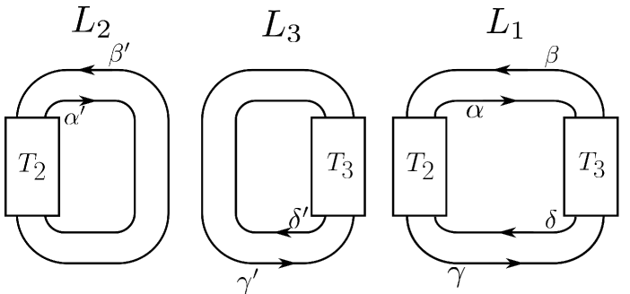
Lemma 2.4.
As shown in Fig.1, consider three link diagrams with arcs and . For any parabolic representation such that and , there are parabolic representations with such that .
Proof.
Define and by and canonically. We consider the bands that connect and (see Fig.2).
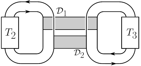
Regard the bands as two oriented disks in the 4-ball such that . Let denote the -fold cyclic covering branched over . By assumption, we have a representation , which induces such that and . Note the homeomorphism given by the construction of branched covering spaces. Hence, by Remark 2.2, we obtain the required equality as follows:
∎
For , let be the -torus link and be the -twist knot (Fig.3). As a corollary,
.

Corollary 2.5.
Let be generic and . Then, for any ,
Proof.
We focus on the proof for the torus links , because the latter claim for the twist knots follows in the same manner as the proof of the former claim for the torus links .
Considering a diagram of the torus link with arcs , as shown in Fig.4, we obtain the following Wirtinger presentation:
| (5) |
.

If we replace in (5) by , then we also get the Wirtinger presentation of .
Let be a parabolic representation. We have
since . Thus, by repeatedly applying Lemma 2.4, there are parabolic representations and such that . Because [Hut13], it follows that
Recalling the proof of Lemma 2.4, one can easily verify that the map , which sends to , is bijective. Hence, . ∎
3 Computation from the quandle cocycle invariant
In this section, we describe a procedure for computing a reduction of the parabolic DW invariant (2) in terms of quandle cocycle invariants. For this, we review the cocycle invariants to compute the reduction (see (6) below). In addition, we compute the reduced invariants of several links; see Section 3.2.
Throughout this section, we assume that the prime power is generic and odd, and fix a non-square number .
3.1 Review of quandle cocycle invariants
First, we review some quandles and colorings. For , let be the quotient of subject to the relation for any The order of is . Define the binary map by
The pair is sometimes called the parabolic quandle (see Example 3.15 in [Nos17]). For a link diagram of a link , an -coloring is a map satisfying the condition on the left diagram of Fig.5 at each crossing of . We further define a shadow coloring to be a pair of an -coloring and a map from the complementary regions of to such that, if the regions and are separated by an arc as shown on the right diagram of Fig.5, the equality holds and the unbounded region is assigned by . Let denote the set of shadow colorings of , and let be . Then, there is a bijection (see, e.g., [Nos17, Example 3.16])

Next, we briefly review the quandle (co)-homology. Let us construct a complex by setting the free -module spanned by , and let its boundary be
The composite is known to be zero. The pair is called the rack complex. Let be a submodule of generated by -tuples with for some . Because , we can define a complex as the quotient complex . The homology is called the quandle homology of . If the prime power is generic, then (see [Nos17, Theorem C.7])
Dually, for an abelian group , we can define the cohomology groups and in terms of the coefficient . For example, any cohomology 3-class in is represented by a map satisfying
for any Such a 3-cocycle is called a quandle 3-cocycle of .
We now briefly review the (shadow) quandle cocycle invariants [CKS01]. Let be a diagram of a link and be a shadow coloring. For the crossing shown in Fig.6, we define the weight of to be , where is the sign of according to Fig.6. Then, the fundamental class of is defined to be ; this is a 3-cycle. We denote the homology class in by . As a corollary of [Nos15] and [Nos17, Corollary 6.20], there is a surjective homomorphism such that
| (6) |
for any . To conclude, the formal sum without -torsion is equivalent to the parabolic DW invariant of the link because annihilates .

However, it is generally difficult to perform this evaluation in the homology . As usual, a quandle 3-cocycle and the pairing are commonly considered; this pairing is often called the quandle cocycle invariant [CKS01]. In conclusion, to compute the parabolic DW invariants (2), it is crucial to find an explicit formula for .
3.2 Quandle 3-cocycles from the Bloch group
In the previous section, using qundle -cocycles, we introduced a procedure for evaluating a reduction of the parabolic DW invariant. While it is generally difficult to find non trivial 3-cocycles, the purpose of this section is to describe a quandle 3-cocycle with ; see Proposition A.1.
First, we review another complex and a chain map defined in [IK14]. Let be a set acted on by . For example, if is either or the projective space , then has a right action on . Consider to be the free -module generated by -tuples , and define the differential map by
Let us define to be the quotient complex This quotient has been extensively studied, e.g., in [Hut13, Section 2].
Next, we introduce a chain map as follows. Let be and let be the zero map. Furthermore, define with by
Because we do not use any chain maps of higher degree, we omit the definition (see [IK14] for details). The map , which is often called the Inoue-Kabaya chain map, induces a homomorphism ; see [IK14, Theorem 3.4]. Thus, if we can find a suitable group and a 3-cocycle of , we obtain a quandle 3-cocycle as the pullback .
Let us review the Bloch group of the finite field . Let be the abelian group presented by generators with subject to the relations
Let denote the quotient of the multiplicative group by the subgroup generated by all . It is easy to check . Consider the canonical homomorphism that sends to . The kernel is called the Bloch group, and is denoted by ; this kernel is isomorphic to (see, e.g., [Hut13, Lemma 7.4]). If , an explicit expression of the isomorphism can easily be obtained with the help of a computer program; see [Kar21b, Appendix A] for . Moreover, let be the quotient group of given by the following relations:
Consider the projection and denote the image of by . When is odd, the following isomorphisms hold (see [Oht, Theorem 4.4] for details):
In particular, if , we can naturally identify with .
Next, we construct a specific homomorphism . For distinct points of , we define
and define a homomorphism by
Because according to [Kar21b, Lemma 4.2] and , the map induces a homomorphism . In summary, we have the following:
Proposition 3.1.
Let be the canonical projection. The following composite map is a quandle 3-cocycle:
In conclusion, because we can specifically describe and with generators, we obtain a detailed presentation of the quandle 3-cocycle . This leads to the following:
Theorem 3.2.
Suppose is a generic prime power. Let be the Bloch-Wigner map, and let be the composite of and the projection . Then, there is an isomorphism such that
3.3 Some computational examples with quandle cocycle invariant
Using Theorem 3.2 and a computer program, we can compute for prime knots with seven or fewer crossings. Table 1 presents the computational results. Here, we do not consider twist knots because the resulting computations have already been presented in [Kar21b], and we omit the case with because .
Proposition 3.3.
(cf. [Kar21b, Theorem 3.1]). Let and be a diagram of . Then and the reduced DW invariant of is computed as
Proof.
It is sufficient to compute the left-hand side for because of Corollary 2.5; with the help of a computer program, we can easily show the required equality. ∎
Note that, for , we can compute the reduced DW invariant of in the same manner.
Appendix A Another definition of parabolic DW invariant
Section 2 defines the parabolic DW invariant with branched coverings. Concerning 3-manifolds with boundaries, there are other approaches to defining 3-manifold invariants like the DW invariant using the relative group homology (see [Nos20, Zic09, Wak92]). However, it is not so easy to approach the (relative) fundamental class of 3-manifolds in terms of the relative group homology.
In the knot case, we can briefly define the DW invariant with the relative group homology. Let us review the relative group homology for groups and a commutative ring . Let be the free -module in which the basis is formed by the elements and define the boundary map by the formula
Furthermore, we define the relative complex by the mapping cone. More precisely, is defined by , and the boundary map is defined by
Then, the relative homology is called the relative group homology of , and is denoted by . If a space pair is an Eilenberg-MacLane space pair, the ordinary homology is known to be isomorphic to .
For example, consider the case where is a knot complement, and is the torus boundary. Then, the integral third homology is isomorphic to , and the generator corresponds with the fundamental class of . In addition, consider a meridian and a preferred longitude in , and suppose there is a homomorphism such that , where is a group and is a subgroup. Then, we can canonically define the pushforward up to sign. Here, the sign depends on the choices of .
To form a comparison with the parabolic DW invariants, we consider the special case of and take as the upper-triangular subgroup. Note that the group isomorphisms if is odd and if is even. In particular, as a result of the transfer map (see [Bro94, §3.9]), we can easily obtain . In addition, when is generic, we have the long exact sequence
Because is annihilated by and , we have the decomposition
| (7) |
Denote the projection by . Then, it is natural to consider the following definition:
| (8) |
Proposition A.1.
Let be a knot , and suppose that is generic. With an appropriate choice of the projection , the definitions of the parabolic DW invariants are equal. That is,
Proof.
Let be . Consider the inclusion , which induces the isomorphisms
according to the homology long exact sequence and the excision axiom. Denote the composite of the isomorphism by . By definition, , leading to for some choice of . Moreover, let be the cyclic covering. Then, . Thus, for any parabolic representation ,
Replacing by , we obtain the required equality from the definitions of the invariants. ∎
Remark A.2.
In (8), we omit the information on the summand in (7). However, the following discussion demonstrates that this information is largely determined by the pair . Because , and can be regarded as 1-cycles in the group homology , and the cross product generates Moreover, from the delta map of the long exact sequence, we can deduce that Thus, . Because the delta map can be regarded as the projection in (7), is almost determined by the pair as required.
A.1 Comparison with reduced DW invariant of Karuo
Next, when is generic, Proposition A.3 states that our invariants in (2) and (8) is a lift of the reduced DW invariant of Karuo [Kar21a, Kar21b].
First, we briefly review the reduced invariant. Let be an open tubular neighborhood of in . Because , every essential simple closed curve on is presented by , where and are coprime. Let us call the -curve. Let be the closed 3-manifold obtained from by the Dehn filling along . Then, for any parabolic representation , the kernel of is non-trivial, because is of infinite order and . Thus, we can choose a coprime pair such that is trivial; therefore, induces . However, the pushforward depends on the choice of .
To obtain knot invariants, Karuo considered the Bloch group and the Bloch-Wigner map ; see [Kar21a, Section 2] for the definitions. Recall the groups and and the map from Section 3.2. Karuo showed that the quotient in is independent of the choice of . Then, the reduced DW invariant of is defined as the sum of the pushforwards over all parabolic representations in . Note that while the reduced DW invariant in [Kar21a, Kar21b] is defined as a formal sum of all conjugacy classes of parabolic representations with respect to the general linear group , this paper defines the reduced DW invariant as a formal sum of all parabolic representations.
Using a similar argument as in the proof of Proposition A.1, we can show the following.
Proposition A.3.
Let be a knot . Suppose is generic. With an appropriate choice of the projection , . In particular, the reduced DW invariant is a specialization of the parabolic DW invariant in (2).
Appendix B Some computations of
For , let be either the -torus link or the -twist knot . Then, the double branched covering space is homeomorphic to a lens space. Hence, we can apply the computational method described in Section 2.2 to . This appendix presents the computational results of and for . Note that, for , the invariants can be easily calculated in a similar manner. In this appendix, we let , and take as the generators of the subgroups , respectively. In addition, we identify with and with .
Acknowledgments I am grateful to my supervisor Takefumi Nosaka for many helpful suggestions. I also thank Hiroaki Karuo for valuable comments.
References
- [BE78] R. Bieri and B. Eckmann, Relative homology and Poincaré duality for group pairs, J. Pure Appl. Algebra 13 (1978), no. 3, 277–319.
- [Bro94] K. S. Brown, Cohomology of groups, Graduate Texts in Mathematics, vol. 87, Springer-Verlag, New York, 1994.
- [CKS01] J. S. Carter, S. Kamada, and M. Saito, Geometric interpretations of quandle homology, Journal of knot theory and its ramifications 10 (2001), no. 03, 345–386.
- [DW90] R. Dijkgraaf and E. Witten, Topological gauge theories and group cohomology, Comm. Math. Phys. 129 (1990), no. 2, 393–429.
- [Hut13] K. Hutchinson, A Bloch-Wigner complex for , J. K-Theory 12 (2013), no. 1, 15–68.
- [IK14] A. Inoue and Y. Kabaya, Quandle homology and complex volume, Geometriae Dedicata 171 (2014), no. 1, 265–292.
- [Kar21a] H. Karuo, The reduced Dijkgraaf-Witten invariant of double twist knots in the Bloch group of , J. Knot Theory Ramifications 30 (2021), no. 7, Paper No. 2150055, 52.
- [Kar21b] , The reduced Dijkgraaf-Witten invariant of twist knots in the Bloch group of a finite field, J. Knot Theory Ramifications 30 (2021), no. 3, Paper No. 2150014, 70.
- [Kim18] Naoki Kimura, A generalization of the dijkgraaf-witten invariants for cusped 3-manifolds, 2018, preprint, arXiv:1805.05130.
- [Nos15] T. Nosaka, Homotopical interpretation of link invariants from finite quandles, Topology and its Applications 193 (2015), 1–30.
- [Nos17] , Quandles and topological pairs, SpringerBriefs in Mathematics, Springer, Singapore, 2017, Symmetry, knots, and cohomology.
- [Nos20] , On the fundamental 3-classes of knot group representations, Geom. Dedicata 204 (2020), 1–24.
- [Oht] T. Ohtsuki, On the bloch groups of finite fields and their quotients by the relation corresponding to a tetrahedral symmetry, preprint, https://www.kurims.kyoto-u.ac.jp/preprint/file/RIMS1938.pdf.
- [Tak59] S. Takasu, Relative homology and relative cohomology theory of groups, J. Fac. Sci. Univ. Tokyo Sect. I 8 (1959), 75–110.
- [Wak92] M. Wakui, On Dijkgraaf-Witten invariant for -manifolds, Osaka J. Math. 29 (1992), no. 4, 675–696.
- [Zic09] C. K. Zickert, The volume and Chern-Simons invariant of a representation, Duke Math. J. 150 (2009), no. 3, 489–532.