Best of Both Worlds:
Regret Minimization versus Minimax Play

Abstract

In this paper, we investigate the existence of online learning algorithms with bandit feedback that simultaneously guarantee $O(1)$ regret compared to a given comparator strategy, and $O(\sqrt{T})$ regret compared to the best strategy in hindsight, where $T$ is the number of rounds. We provide the first affirmative answer to this question. In the context of symmetric zero-sum games, both in normal- and extensive form, we show that our results allow us to guarantee to risk at most $O(1)$ loss while being able to gain $\Omega(T)$ from exploitable opponents, thereby combining the benefits of both no-regret algorithms and minimax play.

1 Introduction

Two-player zero-sum games form one of the most fundamental classes studied in game theory, capturing direct competition between two opposing agents. In a zero-sum game, Alice and Bob choose mixed strategies $\mu\in\mathcal{P}$ and $\nu\in\mathcal{P}$, respectively, for some strategy polytope $\mathcal{P}$. Their expected payoffs are specified by a function $V$. Alice aims to minimize $V(\mu,\nu)$, whereas Bob aims to maximize it. This definition subsumes the classical normal-form zero-sum games (Von Neumann and Morgenstern, 2007, e.g., Rock-Paper-Scissors) as well as the more complex extensive-form zero-sum games (Osborne and Rubinstein, 1994, e.g., Heads-up Poker). A zero-sum game is symmetric if interchanging the actions of the players interchanges payoffs, i.e. $V(\mu,\nu)=-V(\nu,\mu)$.

Now suppose Alice repeatedly plays a symmetric zero-sum game against Bob for $T$ consecutive rounds. In each round, she chooses her next strategy based on her previous observations, and Bob does likewise. There are two popular lines of thought on how Alice could minimize her overall cost over the $T$ rounds of play:

1) Min-Max Equilibrium: In every round $t$, Alice selects $\mu^{t}=\mu^{\star}\in\arg\min_{\mu\in\mathcal{P}}\max_{\nu\in\mathcal{P}}V(\mu,\nu)$ (Von Neumann and Morgenstern, 2007). She then loses at most $V^{\star}:=\min_{\mu\in\mathcal{P}}\max_{\nu\in\mathcal{P}}V(\mu,\nu)$ money. For symmetric zero-sum games, we have $V^{\star}=0$, meaning that:

Alice is guaranteed not to lose any money, but might not win money even if Bob plays poorly.

2) Regret Minimization: Alice selects $\mu^{t}\in\mathcal{P}$ according to a no-regret algorithm Cesa-Bianchi and Lugosi (2006). Then, no matter Bob’s strategies $\nu^{1},\ldots,\nu^{T}\in\mathcal{P}$, the regret compared to any fixed strategy $\mu$ satisfies

$$\sum_{t=1}^{T}V(\mu^{t},\nu^{t})-\sum_{t=1}^{T}V(\mu,\nu^{t})\leq O(\sqrt{T}).$$

In symmetric zero-sum games, plugging in the equilibrium $\mu=\mu^{\star}$, we have $V(\mu,\nu^{t})\leq V^{\star}=0$. This means that Alice might lose up to $O(\sqrt{T})$ money. However, if Bob plays sub-optimally, it may be the case that $\min_{\mu\in\mathcal{P}}\sum_{t=1}^{T}V(\mu,\nu^{t})=-\Theta(T)$, meaning that Alice wins $\Theta(T)$ money. As a result:

Alice risks losing $O(\sqrt{T})$ money, but can win up to $\Theta(T)$ money if Bob plays sub-optimally.

Whether Alice will choose to play 1) a min-max equilibrium or 2) according to a no-regret algorithm depends on how risk-averse Alice is — how willing Alice is to risk $O(\sqrt{T})$ money in the hope of winning $\Theta(T)$. This naturally raises the question of whether we can have the best of both worlds:

Question 1.

In a symmetric zero-sum game, can Alice risk losing at most $O(1)$ amount of money, but still be able to win up to $\Theta(T)$ amount of money if Bob plays sub-optimally?

In this paper, we answer this question in the affirmative by resolving the following fairly more general question from online learning with adversarial linear costs. We explain the reduction in Section˜2.

Question 2.

Is it possible to guarantee $O(1)$ regret compared to a specific strategy while maintaining $\tilde{O}(\sqrt{T})$ regret compared to the best strategy in hindsight?

Question 2 is known to admit a relatively simple positive answer in the so-called full-information case (Section˜1.1). Crucially, in this work we are interested in the bandit feedback setting, modeling the fact that Alice only observes the realized cost and not the cost for all actions she could have taken instead. We formalize this learning goal in Sections˜3.1 and 4.1.

We present our results in the context of symmetric zero-sum games. However, they hold far beyond symmetric, zero-sum, or even two-player games (˜2): for any (sufficiently explorative) comparator strategy, one can guarantee constant regret compared to it while still having rate-optimal regret compared to the best strategy in hindsight, even under bandit feedback.

Contributions. Our main contributions are the following:

• We first devise an algorithm for normal-form games (NFGs) under bandit feedback that interpolates between playing the min-max equilibrium and no-regret learning. We prove that if the min-max equilibrium is supported on the whole action space, then our algorithm indeed satisfies the desiderata of our main question (Section˜3.2). To the best of our knowledge, this is the first result of its kind under bandit feedback.

• We complement this regret guarantee with a lower bound for NFGs, showing that the regret bound cannot be improved significantly (Section˜3.3). This implies that our algorithm is close to optimally exploiting weak strategies, as desired.

• We then transfer our insights to the more challenging framework of extensive-form games (EFGs). This is specifically relevant since in stateful games, it is essential to consider bandit feedback. By proposing a corresponding algorithm for EFGs, we show that even in such interactive games with imperfect information, we can answer our main question in the affirmative (Section˜4.2). We generalize our lower bound to this setting, too (Section˜4.3).

Finally, we numerically evaluate our algorithm in simple EFG environments (Section˜5), showing that our results are not merely of theoretical interest. Indeed, our findings confirm our theoretical insights and demonstrate strong results even when the min-max equilibrium is not full-support.

1.1 Related Work

In online learning under full information feedback, it is known that one can achieve constant regret against a certain comparator strategy while maintaining the optimal worst-case regret guarantee as desired in ˜2 (Hutter et al., 2005; Even-Dar et al., 2008; Kapralov and Panigrahy, 2011; Koolen, 2013; Sani et al., 2014; Orabona and Pál, 2016; Cutkosky and Orabona, 2018; Orabona, 2019), one notable example being the Phased Aggression template of Even-Dar et al. (2008). This allows us to directly answer ˜1 affirmatively for NFGs if full information is available.

In stark contrast, under bandit feedback, Lattimore (2015) showed that constant regret compared to a deterministic comparator strategy (i.e. a single action) is not achievable if we want to maintain sublinear regret compared to all other actions. In Theorem˜3.1, we show that one can break this negative result under the minimal possible assumption on the comparator strategy.

Similar to our motivation, Ganzfried and Sandholm (2015) consider Safe Opponent Exploitation as deviating from the min-max strategy while ensuring at most the cost of the min-max value. The authors provide several such “safe exploitation" algorithms, assuming the existence of so-called “gift strategies". One key difference to our work is that they do not provide a theoretical exploitation guarantee, while our algorithm has provably vanishing regret compared to the best static response against the opponent.

Regarding the extension of our results to EFGs, we leverage relatively recent theoretical advancements regarding online mirror descent in EFGs, most notably Kozuno et al. (2021); Bai et al. (2022). We refer to Appendix˜A for an extended discussion of related work.

2 Preliminaries

In this section, we introduce the relevant notation and explain how Question 2 answers Question 1.

General Notation. As usual, $O$-notation expresses asymptotic behavior, and $\tilde{O}$-notation hides poly-logarithmic factors. The $n$-dimensional simplex is $\Delta_{n}$, and we let $[n]:=\{1,\dots,n\}$. Moreover, $e_{i}$ is the $i$-th the standard basis vector of $\mathbb{R}^{n}$, and $\left\langle\cdot,\cdot\right\rangle$ the Euclidean inner product. Finally, $\mathbbm{1}_{E}$ denotes the indicator function of an event $E$.

(Safe) Online Linear Minimization. In Protocol 1, we introduce the framework of online linear minimization (Hazan, 2019, OLM) with adversarial costs. In addition to this standard framework, Alice receives a special (“safe") comparator strategy $\mu^{c}\in\mathcal{P}$ as input, compared to which Alice would like to be essentially at least as good.

Protocol 1 (Safe) Online Linear Minimization

Special comparator $\mu^{c}\in\mathcal{P}$.

for round $t=1,\dots,T$ do

  Alice chooses her next $\mu^{t}\in\mathcal{P}$, Bob chooses the cost vector $c_{t}$.

  Alice suffers expected cost $\left\langle\mu^{t},c^{t}\right\rangle$. Goal: $\mathcal{R}(\mu^{c})\leq O(1)$ and $\max_{\mu\in\mathcal{P}}\mathcal{R}(\mu)\leq\tilde{O}(\sqrt{T}).$

We define Alice’s expected regret compared to a strategy $\mu\in\mathcal{P}$ by

$$\mathcal{R}(\mu):=\sum_{t=1}^{T}\mathbb{E}\left[\left\langle\mu^{t}-\mu,c^{t}\right\rangle\right].$$

The worst-case expected regret $\max_{\mu}\mathcal{R}(\mu)=\sum_{t=1}^{T}\mathbb{E}\left[\left\langle\mu^{t},c^{t}\right\rangle\right]-\min_{\mu}\sum_{t=1}^{T}\mathbb{E}\left[\left\langle\mu,c^{t}\right\rangle\right]$ then measures the regret compared to the best fixed strategy $\mu$ in hindsight. Under safe OLM (Question 2), we understand the problem of simultaneously guaranteeing

$$\mathcal{R}(\mu^{c})\leq O(1),\quad\text{and}\quad\max_{\mu\in\mathcal{P}}\mathcal{R}(\mu)\leq\tilde{O}(\sqrt{T}).$$ (OLM)

Question 2 Answers Question 1. Now suppose Alice was able to guarantee (OLM). As we explain in Sections˜3.1 and 4.1, both for NFGs and EFGs, we can write the expected cost in round $t$ as a linear function of the strategy, i.e.

$$V(\mu,\nu^{t})=\left\langle\mu,c^{t}\right\rangle$$

for some cost vector $c^{t}$. Alice can now set $\mu^{c}=\mu^{\star}=\arg\min_{\mu}\max_{\nu}V(\mu,\nu)$ to be a min-max equilibrium. Since $V(\mu^{c},\nu)\leq V^{\star}=0$ for symmetric zero-sum games, the first part of (OLM) implies

$$\sum_{t=1}^{T}\mathbb{E}\left[V(\mu^{t},\nu^{t})\right]\leq\sum_{t=1}^{T}\mathbb{E}\left[V(\mu^{c},\nu^{t})\right]+O(1)\leq O(1),$$

no matter Bob’s play. Alice will thus lose at most a constant amount in expectation. Furthermore, if (for example) Bob plays a fixed strategy $\nu^{t}=\nu\in\mathcal{P}$ that is suboptimal in the sense that $\min_{\mu}V(\mu,\nu)=-c<0$, then the second part in (OLM) shows

$$\sum_{t=1}^{T}\mathbb{E}\left[V(\mu^{t},\nu^{t})\right]\leq\min_{\mu}\sum_{t=1}^{T}V(\mu,\nu)+\tilde{O}(\sqrt{T})\leq-\Theta(T),$$

and Alice will linearly exploit Bob. We will thus state our results in terms of safe OLM, keeping in mind that the above reduction will automatically answer our initial ˜1.

3 Normal-Form Games

Suppose Alice and Bob repeatedly play a (symmetric zero-sum) normal-form game for $T$ rounds, which means the following. In each round $t$, they simultaneously submit actions $a^{t},\leavevmode\nobreak\ b^{t}\in[A]$ by sampling from mixed strategies $\mu^{t},\leavevmode\nobreak\ \nu^{t}\in\Delta_{A}$, respectively. Alice receives cost $U_{a^{t},b^{t}}=\left\langle e_{a^{t}},Ue_{b^{t}}\right\rangle$, for some fixed cost matrix $U\in\mathbb{R}^{A\times A}$ with entries in $[0,1]$. We consider bandit feedback, meaning that Alice only observes her cost $U_{a_{t},b_{t}}$ and not the cost of actions she could have taken instead.

3.1 From NFGs to Online Linear Minimization

By defining Alice’s cost function as

$$c^{t}:=Ue_{b^{t}}\in\mathbb{R}^{A},$$

we see that Alice’s expected cost is $V(\mu^{t},\nu^{t}):=\mathbb{E}\left[U_{a_{t},b_{t}}\right]=\mathbb{E}\left[\left\langle\mu,c^{t}\right\rangle\right]$, as $a^{t}\sim\mu^{t}$. We are thus in the setting of OLM (Protocol 1) over $\mathcal{P}=\Delta_{A}$. Notably, Alice does not observe the full cost function $c^{t}$ but only its entry $c^{t}(a^{t})=U_{a^{t},b^{t}}$ at the chosen action (bandit feedback). We formally consider Protocol 2 for any adversarially picked cost functions $c^{t}$. From Section˜2 we know that it is now sufficient to set $\mu^{c}=\mu^{\star}$ and guarantee (OLM).

Protocol 2 Bandit Feedback over the Simplex (NFGs)

Special comparator $\mu^{c}\in\Delta_{A}$.

for round $t=1,\dots,T$ do

  Alice chooses her next action $a^{t}\sim\mu^{t}\in\Delta_{A}$, Bob chooses the cost $c^{t}\in\mathbb{R}^{A}$. $\triangleright\leavevmode\nobreak\$ NFG: $c^{t}=Ue_{b^{t}}$

  Alice suffers and observes cost $c^{t}(a^{t})$. $\triangleright\leavevmode\nobreak\$ NFG: $U_{a^{t},b^{t}}$

3.2 Upper Bound

Our first main result shows that if the special comparator strategy lies in the interior of the simplex, we are able to guarantee constant regret while maintaining low worst-case regret at the optimal rate.

Theorem 3.1.

Let $\delta\in(0,1/A]$. Consider any mixed strategy $\mu^{c}\in\Delta_{A}$ such that $\mu^{c}(a)\geq\delta$ for all $a\in[A]$. Under bandit feedback (Protocol 2), for any $c^{t}\in[0,1]^{A}$, Algorithm˜1 achieves

$$\mathcal{R}(\mu^{c})\leq 1,\quad\text{and}\quad\max_{\mu\in\Delta_{A}}\mathcal{R}(\mu)\leq\tilde{O}\left(\delta^{-1}\sqrt{T}\right).$$

For the case of NFGs, this means that if the min-max strategy $\mu^{\star}$ is full-support, then in expectation: Alice will lose at most $O(1)$ money while winning $\Omega(T)$ money if Bob plays (oblivious) strategies that are linearly exploitable.

Lattimore (2015)’s result implies that the assumption on $\mu^{c}$ is also necessary. In addition, we show in Theorem˜3.2 that a multiplicative dependence on $\delta^{-1}$ is unavoidable. We remark that min-max strategies $\mu^{\star}$ of various zero-sum games are $\delta$-bounded away from zero. For example in Rock-Paper-Scissors $\mu^{\star}=(1/3,1/3,1/3)$. More importantly, even when this is not the case, we remark the following.

Remark 3.1.

Alice can apply the result even in zero-sum games with min-max strategies $\mu^{\star}\in\Delta_{A}$ that are not full-support. Indeed, she can consider the subset of actions $\mathcal{A}^{\prime}:=\{a\in[A]\colon\mu^{\star}(a)>0\}$. Then, our algorithm run on $\mathcal{A}^{\prime}$ still guarantees $\mathcal{R}(\mu^{\star})\leq O(1)$, meaning that Alice can lose at most $O(1)$ in symmetric zero-sum games. At the same time, our algorithm guarantees that $\sum_{t=1}^{T}\mathbb{E}\left[V(\mu^{t},\nu^{t})\right]\leq\min_{\mu\in\Delta^{\prime}}\sum_{t=1}^{T}\mathbb{E}\left[V(\mu,\nu^{t})\right]+\tilde{O}(\sqrt{T})$, where $\Delta^{\prime}$ is the simplex restricted to $\mathcal{A}^{\prime}$. This means that if Bob plays suboptimally, Alice can still guarantee to win $\Theta(T)$ whenever these actions allow her to do so (while $\mu^{\star}$ itself does not guarantee this).

Algorithm 1 Phased Aggression with Importance-Weighting

1:Number of rounds $T$, comparator margin $\delta$, regret upper bound $R\leftarrow\delta^{-1}\sqrt{2T\log(A)}$, OMD learning rates $\eta\leftarrow\sqrt{\delta^{2}\log(A)/(2T)}$, $\tau\leftarrow\sqrt{2\log(A)/(AT)}$.

2:Initialize $\hat{\mu}^{1}(a)\leftarrow\frac{1}{A}$ for all $a\in[A]$, initialize $\alpha\leftarrow 1/R$, $\text{start}\leftarrow 1$, $k\leftarrow 1$ (counts phase).

3:for round $t=1,\ldots,T$ do

4:  Alice chooses $\mu^{t}\in\Delta_{A}$, Bob selects cost $c^{t}$. $\triangleright\leavevmode\nobreak\$in NFGs: $c^{t}=Ue_{b^{t}}$

5:  Alice suffers and observes cost $c^{t}(a^{t})$ for $a^{t}\sim\mu^{t}$.

6:  Alice builds cost estimator $\hat{c}^{t}(a)\leftarrow\frac{c^{t}(a^{t})}{\mu^{t}(a)}\mathbbm{1}\left\{a^{t}=a\right\}$.

7:  if $\max_{\mu\in\Delta_{A}}\sum^{t}_{j=\text{start}}\left\langle\hat{c}^{j},\mu^{c}-\mu\right\rangle>2R$ and $\alpha<1$ then

8:   $k\leftarrow k+1$, $\text{start}\leftarrow t+1$. $\triangleright\leavevmode\nobreak\$If comparator performs poorly, new phase

9:   $\hat{\mu}^{t+1}(a)\leftarrow\frac{1}{A}$ for all $a\in[A]$. $\triangleright\leavevmode\nobreak\$Re-initialize OMD

10:   Update $\alpha\leftarrow\min\left\{2^{k-1}/R,\leavevmode\nobreak\ 1\right\}$. $\triangleright\leavevmode\nobreak\$Increase $\alpha$ for upcoming phase

11:  else$\triangleright\leavevmode\nobreak\$OMD update

12:   $\hat{\mu}_{x}^{t+1}\leftarrow\arg\min_{\mu\in\Delta_{A}}\left(\eta^{\prime}\left\langle\mu,\hat{c}^{t}\right\rangle+D_{\text{KL}}(\mu||\hat{\mu}^{t})\right)$, with $\eta^{\prime}=\eta$ if $\alpha<1$, and $\eta^{\prime}=\tau$ if $\alpha=1$.   

13:  $\mu^{t+1}\leftarrow\alpha\hat{\mu}^{t+1}+\left(1-\alpha\right)\mu^{c}$. $\triangleright\leavevmode\nobreak\$Play shifted OMD to $\mu^{c}$ by $1-\alpha$

Our Algorithm. In this section, we present Algorithm˜1 and explain its key steps. Our algorithm is inspired by the Phased Aggression algorithm, originally proposed by Even-Dar et al. (2008) for the full-information setting. We briefly note that a direct application of existing full-information algorithms is not possible. This is because, in the bandit setting, Alice only observes her realized cost and not the cost of the other possible actions she could have chosen. We will thus combine the phasing idea of Even-Dar et al. (2008) with appropriately importance-weighted estimators of the full cost function.

We now give an outline of Algorithm˜1. In every round $t$, the Phased Aggression algorithm plays a convex combination between the comparator strategy $\mu^{c}$ and the strategy $\hat{\mu}^{t}$ chosen by a no-regret algorithm (which runs in parallel). That is, the played strategy is $\mu^{t}=\alpha\hat{\mu}^{t}+(1-\alpha)\mu^{c}$ for some $\alpha\in(0,1]$. Whenever the algorithm estimates that the comparator $\mu^{c}$ is a poor choice, it increases $\alpha$ by a factor of two (so that it puts less weight on $\mu^{c}$ and more on the no-regret iterates) and restarts the no-regret algorithm. We group all rounds according to these restarts and call them phases $k=1,2,\dots$. During each phase, $\alpha$ is constant.

Within this phasing scheme, the specifics of our algorithm are as follows. The no-regret algorithm of our choice is standard online mirror descent (Hazan, 2019, OMD). In every round $t$, the algorithm plays its current action $a^{t}\sim\mu^{t}$ and observes its cost (Line 5). It uses this to construct an importance-weighted estimator $\hat{c}^{t}$ of the (unobserved) full cost function (Line 6). The algorithm then performs one iteration of OMD with the estimated costs (Line 12). This procedure is repeated until a new phase is started (Line 7), which happens if the comparator $\mu^{c}$ is performing poorly under the estimated $\hat{c}^{t}$’s of the current phase.

Regarding computation, the OMD update can be implemented in closed form as $\hat{\mu}^{t+1}(a)\propto\hat{\mu}^{t}(a)\exp(-\eta^{\prime}\hat{c}^{t}(a))$. We can check the if-condition in Line 7 by directly computing the maximum in $O(A)$ time.

Regret Analysis. In this section we provide a proof sketch of Theorem 1. We defer the full proof to Section˜B.1.

We first introduce some notation. We index the variables by their respective phase $k\geq 1$: Phase $k$ lasts from $\text{start}_{k}$ to $\text{start}_{k+1}-1$ and uses linear combinations with $\alpha^{k}=\min\{1,2^{k-1}/R\}$ (Lines 8, 10). By design, there are at most $1+\lceil\log_{2}(R)\rceil$ phases, where $R$ is a known regret upper bound for OMD input to the algorithm. The overall regret is at most the sum of regrets across all phases, and we will thus analyze each phase separately. To this end, let

$$\hat{\mathcal{R}}^{k}(\mu):=\sum_{t=\text{start}_{k}}^{\text{start}_{k+1}-1}\left\langle\hat{c}^{t},\mu^{t}-\mu\right\rangle$$

denote the estimated regret during phase $k$. The following lemma bounds this estimated regret for phases with $\alpha^{k}<1$.

Lemma 3.1 (During normal phases).

Let $k$ be such that $\alpha^{k}<1$. Then for all $\mu\in\Delta_{A}$,

$$\hat{\mathcal{R}}^{k}(\mu)\leq 2R+2=2\delta^{-1}\sqrt{2T\log(A)}+2,$$

and for the special comparator $\hat{\mathcal{R}}^{k}(\mu^{c})\leq 2^{k-1}$.

The first part of the theorem establishes a worst-case bound on the estimated regret. Such a bound would normally not be possible for importance-weighted cost estimators. In our case, during phases with $\alpha^{k}<1$, we put constant weight on the comparator strategy $\mu^{c}$, which in turn is lower bounded by $\delta>0$. Our estimated costs (Line 6) will thus be upper bounded, which is a key step in the proof. The second part of the theorem easily follows using the definition of $\alpha^{k}$.

Next, suppose the algorithm exits a phase $k$ as the if-condition in Line 7 holds. The following lemma establishes that exiting the phase is justified in the sense that we perform sufficiently well compared to the special comparator, according to the estimated costs.

Lemma 3.2 (Exiting a phase).

Let $k$ be such that $\alpha^{k}<1$. If Algorithm˜1 exits phase $k$, then $\hat{\mathcal{R}}^{k}(\mu^{c})\leq-2^{k-1}$.

We are now ready to prove Theorem˜3.1. First, consider the case that $\alpha=1$ is never reached. Note that our cost estimates are unbiased, i.e. $\mathbb{E}\left[\hat{c}^{t}(a)\right]=c^{t}(a)$. It is thus sufficient if we can bound $\hat{\mathcal{R}}^{k}$. As there are $O(\log R)$ phases, Lemma˜3.1 implies $\max_{\mu}\mathcal{R}(\mu)\leq O(R\log R)$. Moreover, the previous two lemmas geometrically balance the regret compared to $\mu^{c}$ to be at most $1$, and we conclude. Second, suppose now that $\alpha=1$ is reached. The final phase will then simply be OMD with standard importance-weighting (a.k.a. Exp3), as we put no weight on the special comparator $\mu^{c}$. While we cannot apply Lemma˜3.1, we can directly bound the remaining expected regret of Exp3 (Orabona, 2019). We can thus use the same argument as before, with one additional phase.

3.3 Lower Bound

We will now show that regarding the guarantee we provided in Theorem˜3.1, a multiplicative dependence on the inverse of the “exploration gap" $\delta$ is indeed unavoidable.

Theorem 3.2.

Let $\delta\in(0,1/A]$. There is a comparator $\mu^{c}\in\Delta_{A}$ with all $\mu^{c}(a)\geq\delta$ such that for any algorithm for Protocol 2 there is a sequence $c^{1},\dots,c^{T}\in[0,1]^{A}$ such that: If $\mathcal{R}(\mu^{c})\leq O(1)$, then

$$\max_{\mu\in\Delta_{A}}\mathcal{R}(\mu)\geq\Omega(\sqrt{\delta^{-1}T}-\delta^{-3/4}T^{1/4}).$$

In the context of symmetric zero-sum games, our lower bound establishes that in expectation: If Alice is willing to lose at most $O(1)$ money, the best she can hope to gain from any (fixed) exploitable strategy is $\Theta(T)-\Omega(\delta^{-1/2}\sqrt{T})$.

The key idea of our proof is that any algorithm with low regret compared to $\mu^{c}=(1-\delta,\delta)$ for $A=2$ actions will need to play action 1 most of the time if one can information-theoretically not detect that action 2 is, in fact, minimally better. We defer the proof to Section˜B.2.

4 Extensive-Form Games

In this section, we present our results for EFGs. We start by giving the definition of EFGs that appears in Kozuno et al. (2021); Bai et al. (2022); Fiegel et al. (2023a, b), see Section˜C.1 for a brief discussion. For clarity, we present the two-player, symmetric zero-sum case, although our results readily generalize to arbitrary EFGs.

Definition 4.1.

An EFG is a tuple $(H,\mathcal{S},\mathcal{X},\mathcal{A},P,x,y,u)$, where

• there are $2$ players, Alice and Bob. $\mathcal{A}=[A]$ denotes the set of possible actions for both players.

• $\mathcal{S}$ denotes the set of states of the game. $H\in\mathbb{N}$ is the horizon of the game. At stage $h\in[H]$, $\mathcal{S}_{h}\subseteq\mathcal{S}$ denotes the possible states.

• $P:=(p_{0},p)$ is the transition kernel; the game’s state is sampled according to $s_{h+1}\sim p(\cdot|s_{h},a_{h},b_{h})$ upon actions $a_{h},b_{h}\in\mathcal{A}\times\mathcal{A}$ in state $s_{h}\in\mathcal{S}$. The initial state is sampled according to $s_{1}\sim p_{0}\in\Delta_{\mathcal{S}}$.

• $u(s,a,b)\in[-1,1]$ is Alice’s random cost (Bob’s reward) for actions $(a,b)\in\mathcal{A}\times\mathcal{A}$ chosen in state $s\in\mathcal{S}$, with mean $\bar{u}(s,a,b)$.

• Alice (resp. Bob) observes information sets (infosets) from $\mathcal{X}$ ($|\mathcal{X}|=X$). Infosets are described by a surjective function $x\colon\mathcal{S}\to\mathcal{X}$ (resp. $y\colon\mathcal{S}\to\mathcal{X}$).

The idea behind infosets is that Alice (resp. Bob) has imperfect information about the state of the game: she cannot differentiate between sates $s,s^{\prime}\in\mathcal{S}$ that belong at the same infoset, i.e. when $x(s)=x(s^{\prime})$. This is reflected in the definition of her policy set.

Definition 4.2.

A policy is a mapping $\pi\colon\mathcal{X}\to\Delta_{A}$. We denote the set of all such policies by $\Pi$.

We let $\pi(a|x)$ denote the probability of playing action $a\in\mathcal{A}$ in states $s\in\mathcal{S}$ from infoset $x=x(s)\in\mathcal{X}$. As Alice cannot differentiate between states $s,s^{\prime}\in\mathcal{S}$ from the same infoset, she must act the same way if $x(s)=x(s^{\prime})$.

Definition 4.3.

Given policies $(\pi_{A},\pi_{B})\in\Pi\times\Pi$, the expected total cost for Alice equals

$$V(\pi_{A},\pi_{B}):=\mathbb{E}\left[\sum_{h=1}^{H}u(s_{h},a_{h},b_{h})\right],$$

where $(s_{h},a_{h},b_{h})$ are the state and actions at stage $h\in[H]$ via $a_{h}\sim\pi_{A}(\cdot|x(s_{h}))$, $b_{h}\sim\pi_{B}(\cdot|y(s_{h}))$, and $s_{h+1}\sim p(\cdot|s_{h},a_{h},b_{h})$.

For the remainder of the section, we make the following assumptions, which are standard in the EFG literature (Kozuno et al., 2021; Bai et al., 2022; Fiegel et al., 2023a, b).

Assumption 4.1.

• Tree structure: For any state $s_{h}\in\mathcal{S}_{h}$, there exists a unique sequence $(s_{1},a_{1},b_{1},\dots,\allowbreak s_{h-1},a_{h-1},b_{h-1})$ leading to $s_{h}$.

• Perfect recall: Let $s,s^{\prime}$ such that $x(s)=x(s^{\prime})$. Then:

  • There exists $h\in[H]$ such that $s,s^{\prime}\in\mathcal{S}_{h}$.

  • Let $(s_{1},a_{1},\dots,s_{h-1},a_{h-1})$ be the unique path leading to $s$ and $(s^{\prime}_{1},a^{\prime}_{1},\dots,s^{\prime}_{h-1},a^{\prime}_{h-1})$ the unique path leading to $s^{\prime}$. Then for all $k\in[h-1]\colon x(s_{k})=x(s^{\prime}_{k})$ and $a_{k}=a^{\prime}_{k}$.

Tree structure states that the game proceeds in rounds during which the players cannot loop back to a previous state. Perfect recall establishes that the players never forget the history of play. They can only consider two states as the same infoset if the observations so far have been the same Hoda et al. (2010). The latter implies that infosets are partitioned along the horizon, i.e. $\mathcal{X}=\mathop{\vphantom{\bigcup}\mathchoice{\ooalign{$\displaystyle\bigcup$\cr\raise-8.33339pt\hbox{\set@color\scalebox{1.5}{$\displaystyle\cdot$}}}}{\ooalign{$\textstyle\bigcup$\cr\raise-8.33339pt\hbox{\set@color\scalebox{1.5}{$\textstyle\cdot$}}}}{\ooalign{$\scriptstyle\bigcup$\cr\raise-5.83337pt\hbox{\set@color\scalebox{1.5}{$\scriptstyle\cdot$}}}}{\ooalign{$\scriptscriptstyle\bigcup$\cr\raise-4.16669pt\hbox{\set@color\scalebox{1.5}{$\scriptscriptstyle\cdot$}}}}}_{h\in[H]}\mathcal{X}_{h}$, and the same holds for the states.

Online Learning in EFGs. Now suppose Alice and Bob repeatedly play an EFG for $T$ consecutive rounds. In each round $t\in[T]$, Alice and Bob select a pair of policies $(\pi_{A}^{t},\pi_{B}^{t})\in\Pi\times\Pi$. Then a trajectory $(s_{1}^{t},a_{1}^{t},b_{1}^{t},u_{1}^{t},\dots,s_{H}^{t},a_{H}^{t},b_{H}^{t},u_{H}^{t})$ is sampled according to the policies $(\pi_{A}^{t},\pi_{B}^{t})$ and Alice suffers cost $\sum_{h=1}^{H}u_{h}^{t}$, as summarized in Protocol 3.

Protocol 3 Bandit Feedback over Policies (EFGs)

A comparator policy $\pi^{c}\in\Pi$.

for round $t=1,\dots,T$ do

  Alice selects $\pi_{A}^{t}\in\Pi$, Bob selects $\pi_{B}^{t}\in\Pi$.

  Alice obtains costs $\sum_{h=1}^{H}u_{h}^{t}$ and observes trajectory $(x_{1}^{t},a_{1}^{t},u_{1}^{t},\dots,x_{H}^{t},a_{H}^{t},u_{H}^{t})$.

We remark in EFGs, we are naturally in the bandit feedback setting as Alice only observes the trajectory $(x_{1}^{t},a_{1}^{t},u_{1}^{t},\dots,x_{H}^{t},a_{H}^{t},u_{H}^{t})$. Under full-information feedback, Alice would observe Bob’s actual policy $\pi_{B}^{t}\in\Pi$.

Remark 4.1 (Importance of bandit feedback in EFGs).

In EFGs, bandit feedback is considerably more natural than full-information feedback. This is due to the fact that when playing against Bob, the realized samples are only observed along one single trajectory in the game tree. Observing full information would thus mean knowing Bob’s counterfactual policy in states that have never been visited during play, which is not realistic.

4.1 From EFGs to Online Linear Minimization

As mentioned, we once more resort to the more general OLM problem. Yet this time, our strategy polytope will be the so-called treeplex $\mathcal{P}=\mathcal{T}$ rather than the simplex. The following definition provides an equivalent characterization of a policy. It will allow us to view the expected cost $V(\pi^{t}_{A},\pi^{t}_{B})$ as a (bi-)linear function (Hoda et al., 2010).

Definition 4.4.

A vector $\mu\in\mathbb{R}^{X\cdot A}$ belongs to the treeplex $\mathcal{T}$ iff for all $x_{h}\in\mathcal{X}_{h}$ and $a\in\mathcal{A}$,

$$\begin{cases}\mu(x_{h},a)\geq 0,\\ \sum_{a_{h}\in\mathcal{A}}\mu(x_{h},a_{h})=\mu(x_{h-1},a_{h-1}),\end{cases}$$ (1)

where $(x_{h-1},a_{h-1})$ is the unique predecessor pair reaching $x_{h}$. We consider $\mu(x_{0},a_{0})=1$ for the root by convention.

Remark 4.2.

There is the following equivalence between Definitions˜4.2 and 4.4. Given a policy $\pi\in\Pi$, we can define a unique $\mu_{\pi}\in\mathcal{T}$ by $\mu_{\pi}(x_{h},a_{h})=\prod_{h^{\prime}=1}^{h}\pi(a_{h^{\prime}}|x_{h^{\prime}})$, where the $(x_{h^{\prime}},a_{h^{\prime}})$ form the unique path to $(x_{h},a_{h})$. Vice-versa, given $\mu\in\mathcal{T}$, we can recover the corresponding policy via $\pi_{\mu}(a|x)=\mu(x,a)/\sum_{a^{\prime}}\mu(x,a^{\prime})$.

By convention, we thus identify policies $(\pi_{A}^{t},\pi_{B}^{t})$ with their corresponding treeplex strategies $(\mu^{t},\nu^{t})$ and write $V(\mu^{t},\nu^{t})$ for Alice’s expected cost. The following lemma shows that this definition indeed allows us to view Protocol 3 as a (safe) OLM problem (Protocol 1).

Lemma 4.1.

For any state $s\in\mathcal{S}_{h}$, infoset $x=x(s)\in\mathcal{X}_{h}$ and action $a\in\mathcal{A}$, let $(s_{1},a_{1},b_{1},\dots,s_{h-1},a_{h-1},b_{h-1})$ be the unique path leading to $s$. Let $p(s):=p_{0}(s_{1})\prod_{1\leq h^{\prime}\leq h-1}p(s_{h^{\prime}+1}|s_{h^{\prime}},a_{h^{\prime}},b_{h^{\prime}})$, and consider

$$c^{t}(x,a):=\sum_{\begin{subarray}{c}s\colon x(s)=x,\\ b\in\mathcal{A}\end{subarray}}p(s)\cdot\nu^{t}(y(s),b)\cdot\bar{u}(s,a,b).$$ (2)

Then $V(\mu,\nu^{t})=\left\langle\mu,c^{t}\right\rangle$ for all $\mu\in\mathcal{T}$.

Alice does not observe the full cost function $c^{t}$, as we are in the bandit feedback setting. Yet, this lemma establishes that Protocol 1 over the treeplex $\mathcal{P}=\mathcal{T}$ covers EFGs. Thus, it is sufficient to solve the safe OLM problem (OLM).

4.2 Upper Bound

As in the simplex case, our Algorithm 2 guarantees Eq.˜OLM for any policy $\mu^{c}\in\mathcal{T}$ that is $\delta$-bounded away from the boundary of the strategy polytope. Once more, we can resort to a restricted action set to relax this assumption (Remark˜3.1).

Theorem 4.1.

Let $\delta\in(0,1/A]$. For any special comparator $\mu^{c}\in\mathcal{T}$ such that $\mu^{c}(x,a)\geq\delta$ for all $x$, $a$, Algorithm˜2 achieves (for any $c^{t}$’s from Eq.˜2)

$$\mathcal{R}(\mu^{c})\leq 1,\quad\text{and}\quad\max_{\mu\in\mathcal{T}}\mathcal{R}(\mu)\leq\tilde{O}\left(\delta^{-1}\sqrt{XH^{3}T}\right).$$

Algorithm 2 Phased Aggression with Importance-Weighting for EFGs

1:Number of rounds $T$, comparator margin $\delta$, regret bound $R\leftarrow\delta^{-1}\sqrt{8XH^{3}\log(A)T}$, learning rate $\eta\leftarrow\sqrt{\delta^{2}X\log(A)/(8H^{2}T)}$, balanced learning rate $\tau\leftarrow\sqrt{XA\log(A)/(H^{3}T)}$.

2:Initialize $\hat{\mu}^{1}(x_{h},a)\leftarrow\frac{1}{A^{h}}$ ($h\in[H]$, $x_{h}\in\mathcal{X}_{h}$, $a\in\mathcal{A}$), initialize $\alpha\leftarrow 1/R$, $\text{start}\leftarrow 1$, $k\leftarrow 1$ (counts phase).

3:for round $t=1,\dots,T$ do

4:  Alice chooses $\mu^{t}\in\mathcal{T}$, Bob selects strategy $\nu^{t}\in\mathcal{T}$. $\triangleright\leavevmode\nobreak\$and thus cost $c^{t}$ via Eq.˜2

5:  Alice obtains costs $\sum_{h=1}^{H}u^{t}_{h}$, observes $(x_{1}^{t},a_{1}^{t},u_{1}^{t},\dots,x_{H}^{t},a_{H}^{t},u_{H}^{t})$. $\triangleright\leavevmode\nobreak\$$V(\mu^{t},\nu^{t})$ in exptn.

6:  Alice builds cost estimator $\hat{c}^{t}(x_{h},a)\leftarrow\frac{\mathbbm{1}\{(x_{h}^{t},a_{h}^{t})=(x_{h},a)\}u^{t}_{h}}{\mu^{t}(x_{h},a)}$.

7:  if $\max_{\mu\in\mathcal{T}}\sum^{t}_{j=\text{start}}\left\langle\hat{c}^{j},\mu^{c}-\mu\right\rangle>2R$ and $\alpha<1$ then

8:   $\text{start}\leftarrow t+1$, $k\leftarrow k+1$. $\triangleright\leavevmode\nobreak\$If comparator performs poorly, next phase

9:   $\hat{\mu}^{t+1}(x_{h},a)\leftarrow\frac{1}{A^{h}}$ ($h\in[H]$, $x_{h}\in\mathcal{X}_{h}$, $a\in\mathcal{A}$). $\triangleright\leavevmode\nobreak\$Initialize to uniform policy

10:   Update $\alpha\leftarrow\min\left\{2^{k-1}/R,\leavevmode\nobreak\ 1\right\}$. $\triangleright\leavevmode\nobreak\$Increase $\alpha$ for upcoming phase

11:  else$\triangleright\leavevmode\nobreak\$OMD update

12:   

$$\hskip-82.51282pt\hat{\mu}^{t+1}\leftarrow\begin{cases}\arg\min_{\mu\in\mathcal{T}}\left(\eta\left\langle\mu,\hat{c}^{t}\right\rangle+D(\mu||\hat{\mu}^{t})\right)\quad\quad&\text{(if $\alpha<1$)},\\ \arg\min_{\mu\in\mathcal{T}}\left(\tau\left\langle\mu,\hat{c}^{t}\right\rangle+D^{\text{bal}}(\mu||\hat{\mu}^{t})\right)\quad\quad&\text{(if $\alpha=1$)}.\end{cases}$$ (3)

  

13:  $\mu^{t+1}\leftarrow\alpha\hat{\mu}^{t+1}+\left(1-\alpha\right)\mu^{c}$. $\triangleright\leavevmode\nobreak\$Play shifted OMD to $\mu^{c}$ by $1-\alpha$

Remark 4.3.

The dependence on $X$ is as good as desired in the sense that there is a $\sqrt{XAT}$ lower bound in the unconstrained case. The dependence on $H$ is less crucial for many relevant EFGs, as we often have $X\simeq A^{H}$ and so $H$ is a logarithmic factor. See Bai et al. (2022).

Our Algorithm. Algorithm˜2 is similar to our algorithm for the simplex. It combines the Phased Aggression scheme with importance-weighted OMD. However, in the EFG case, we have to generalize these notions to the treeplex.

In particular, we use OMD with the so-called dilated KL divergence as regularizer (Line 12). As we will see in the regret analysis, to this end it is crucial that we use an unbalanced dilated KL divergence $D$ (Kozuno et al., 2021) in the phases with $\alpha<1$ and a balanced KL divergence $D^{\text{bal}}$ (Bai et al., 2022) if $\alpha=1$ is reached. In Section˜C.2, we formally define the divergences and confirm that they allow for an efficient closed-form implementation. This is crucial as we want to avoid costly projections onto the treeplex by any means. Moreover, we can efficiently check Line 7 via standard dynamic programming over the set of policies.

Regret Analysis. Our analysis follows a similar argument as in Section˜3 and we defer the proofs to Section˜C.3. The main technical challenge is to transfer the regret bounds for importance-weighted OMD from the simplex (with KL) to the treeplex $\mathcal{T}$ (with dilated KL).

In addition, we now require a careful analysis to obtain the best possible dependence on the number of infosets $X$ and actions $A$, in the following sense. First, when upper bounding the estimated regret in analogy to Lemma˜3.1 ($\alpha<1$), we analyze OMD with the unbalanced dilated KL divergence by adapting the argument of Kozuno et al. (2021) to our importance-weighting. Using the (more sophisticated) balanced KL here would introduce an additional undesired factor of $\sqrt{A}$. Second, once $\alpha=1$ in the final phase, we analyze the expected regret of balanced OMD instead, by adapting the argument of Bai et al. (2022) to our cost estimators. Using the unbalanced divergence would introduce an extra factor of $\sqrt{X}$, which can be prohibitively large.

4.3 Lower Bound

As in the case of NFGs, we show that our guarantees for Algorithm˜2 are close to being tight for EFGs of arbitrary depth. Our proof reduces an EFG of depth $H$ to the simplex case from Theorem˜3.2. See Section˜C.5 for the proof.

Theorem 4.2.

Let $A\geq 2$, $H\geq 1$, and $\delta\in(0,1)$. There exists an EFG of depth $H$ with $X=\Theta(A^{H})$ such that for any $\mu^{c}\in\mathcal{T}$ with $\min_{x,a}\mu^{c}(x,a)=\delta$, there is an adversary such that for any algorithm: If $\mathcal{R}(\mu^{c})\leq O(1)$, then

$$\max_{\mu\in\mathcal{T}}\mathcal{R}(\mu)\geq\Omega(\sqrt{\delta^{-1}T}-\delta^{-3/4}T^{1/4}).$$

5 Experimental Evaluations

We experimentally compare our Algorithm˜2 for EFGs to the standard OMD algorithm with dilated KL (Kozuno et al., 2021) as well as to minimax play. Our evaluations confirm our theoretical findings, revealing that Algorithm˜2 achieves the best of both no-regret and minimax play. We provide further details in Appendix˜D.

Kuhn Poker. We consider Kuhn poker (Kuhn, 1950), which serves as a simple yet fundamental example of two-player zero-sum imperfect information EFGs. Kuhn poker is a common $3$-card simplification of standard poker, where each player selects one card from the deck $\{$Jack, Queen, King$\}$ without replacement and initially bets one dollar.

Remark 5.1.

The min-max equilibrium of Kuhn Poker is not full-support ($\delta=0$ in Theorem˜4.1). As seen in Remark˜3.1, we can easily circumvent this issue by considering only the actions in the support of the equilibrium. For Kuhn Poker, this results in $\delta=1/3$. Algorithm˜2 is then still guaranteed not to lose any money while being able to compete with the best response within the support of the equilibrium.

We consider the following baseline algorithms Alice could play over $T$ rounds of Kuhn poker: 1) play the Min-Max equilibrium $\pi^{\star}$ in every round; or 2) run OMD with dilated KL; or 3) run Algorithm˜2 with comparator policy $\pi^{\star}$.

We consider two types of experiments: First, we run the three algorithms against each other to check which of the algorithms risks losing money. Second, we evaluate how well each algorithm allows Alice to exploit exploitable strategies. We repeat each experiment $5$ times.

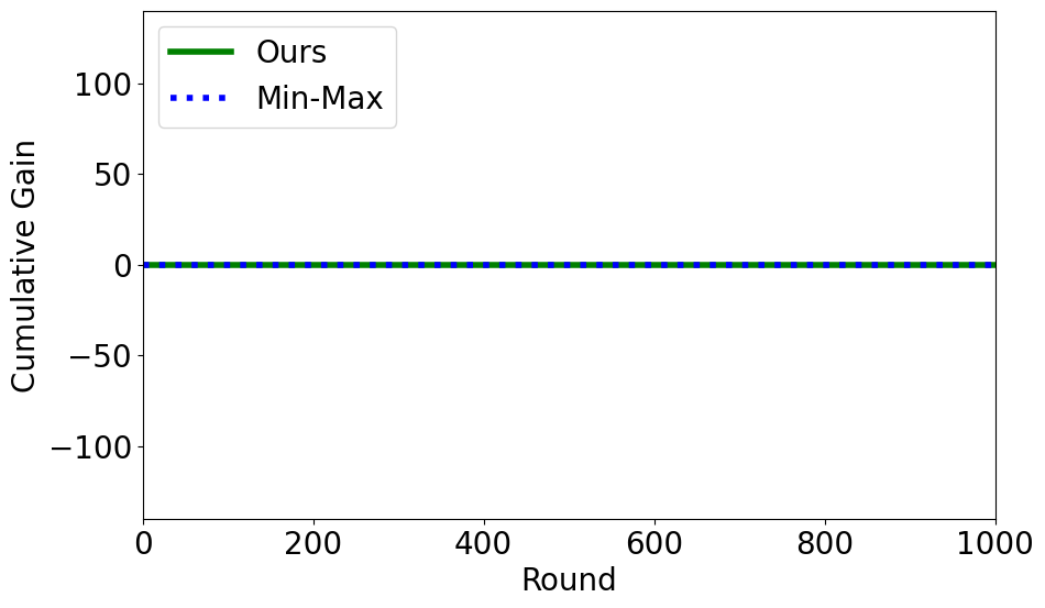
Figure 1: Alg. 2 vs Min-Max

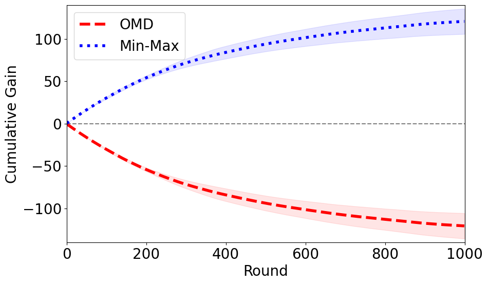
OMD vs Min-Max

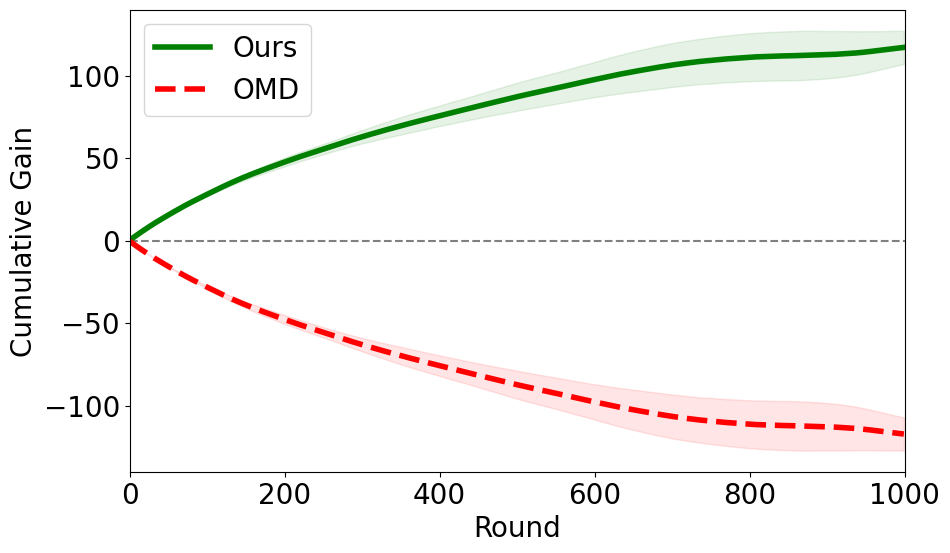
Alg. 2 vs OMD

Figure 2: All vs all comparison for $T=1000$ rounds. The x-axis displays the round $t$, and the y-axis displays how much the respective algorithm (Min-Max, OMD, Algorithm˜2) gained from the other.

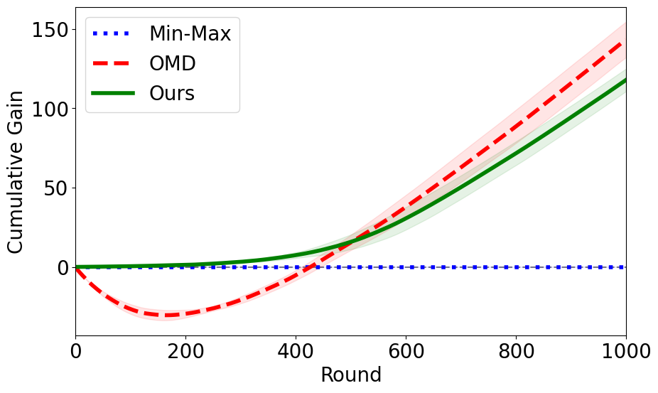
All vs BluffJ

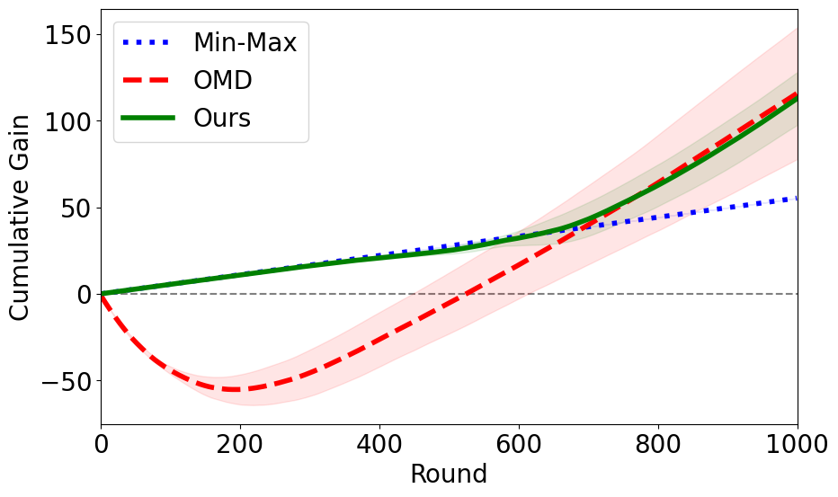
All vs RaiseKQ

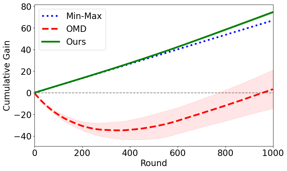
All vs RandMinMax

Figure 3: All vs Bob comparison for $T=1000$ rounds. The x-axis displays the round $t$, and the y-axis displays how much Min-Max, OMD, and Algorithm˜2 gained from the second algorithm so far. The y-axes have varying scales for readability.

All vs All. In Fig.˜2 we plot the total amount of money each algorithm wins. As Fig.˜2 shows, both Min-Max and Algorithm˜2 never incur losses while both gain a significant amount of money against OMD. Indeed, as (symmetrized) Kuhn poker is a symmetric zero-sum game, the min-max equilibrium is guaranteed not to lose. The same holds for our Algorithm˜2. In contrast, a no-regret algorithm such as OMD can lose up to $O(\sqrt{T})$ amount of money. Interestingly, it does lose a similar amount against our Algorithm˜2.

All vs Exploitable Strategies. We now compare the performance of Min-Max, OMD and Algorithm˜2 against the following reasonable but suboptimal strategies. The goal is to understand their ability to exploit weak strategies. We consider a) BluffJ: Bob plays the min-max equilibrium, except that he bets (bluffs) when he has a Jack; b) RaiseKQ: Bob raises/calls if and only if he has a King or a Queen, and checks/folds otherwise; c) RandMinMax: Each round, with probability $0.2$, he plays the uniform strategy, and else the min-max one.

In Fig.˜3 we present the amount of money each algorithm wins against these exploitable strategies. We first consider All vs BluffJ & All vs RaiseKQ. Algorithm 2 plays conservatively and gains an amount similar to Min-Max until it takes off and starts exploiting Bob near-optimally, as OMD would. OMD, in turn, first loses a certain amount of money and only matches the gain of Min-Max after exploring sufficiently, then having the same slope as Algorithm˜2. The min-max equilibrium itself does not exploit BluffJ at all and exploits RaiseKQ sub-optimally. Our algorithm suffers neither of the two drawbacks of losing money or not exploiting the weak strategy. Finally, in All vs RandMinMax, our Algorithm˜2 improves slightly over Min-Max. OMD gains at the same rate after losing an initial amount.

6 Conclusion

In this paper, we showed how to provably exploit suboptimal strategies with essentially no expected risk in repeated zero-sum games by combining regret minimization and minimax play. More generally, we believe that our novel results for adversarial bandits leading to these guarantees may be of independent interest. We hope that our work inspires future research on safe online learning, including settings like convex-concave games, learning with feedback graphs, and establishing no-swap-regret guarantees.

Appendix A Further Related Work

Safe Opponent Exploitation. While there have been some approaches to safe learning in games (Ponsen et al., 2011; Farina et al., 2019; Zhang and Sandholm, 2021; Bernasconi-de Luca et al., 2021; Bernasconi et al., 2022; Ge et al., 2024), all these works are fairly different from our learning problem. Related to Ganzfried and Sandholm (2015); Ganzfried and Sun (2018), the works of Damer and Gini (2017); Liu et al. (2022) provide algorithms that interpolate between being safe and exploitive through a specific parameter. However, these algorithms may incur up to $\Omega(T)$ regret compared to the best fixed strategy in hindsight. Recently, Maiti et al. (2023) proved the first instance-dependent poly-logarithmic regret bound for noisy $2\times 2$ NFGs, which naturally relates to our desired regret bound. However, such bounds become vacuous when the game matrix does not have pairwise distinct entries and assume to observe the opponent’s action (which corresponds to full information in our feedback model).

Exploiting Adaptive Opponents. If Bob is oblivious and plays a fixed sequence of (mixed) strategies, then any regret Alice incurs is potential utility she could gain by playing a no-regret strategy (e.g., the best-of-both-worlds strategy we present). However, if Bob is adaptive, switching to a no-regret strategy does not necessarily allow Alice to recover additional utility (Bob could, for example, react to this by playing his minimax strategy). There is a line of recent work (Deng et al., 2019; Mansour et al., 2022; Kolumbus and Nisan, 2022b, a; Brown et al., 2023; Cai et al., 2023; Chen and Lin, 2023; Haghtalab et al., 2024; Ananthakrishnan et al., 2024; Guruganesh et al., 2024; Arunachaleswaran et al., 2024) on how to play against sub-optimal adaptive strategies (e.g. other learning algorithms) in various settings, although almost all of this work only pertains to general sum games. It is an interesting open question to understand to what extent we can obtain similar best-of-both-worlds results for adaptive opponents in zero-sum games.

Comparator-Adaptive OL with Full Information. In OL under full information feedback, Hutter et al. (2005); Even-Dar et al. (2008); Kapralov and Panigrahy (2011); Koolen (2013); Sani et al. (2014) establish (with various emphases) that safe OLM over the simplex in the sense of Eq.˜OLM is possible. Using so-called parameter-free methods from the online convex optimization literature instead (Orabona and Pál, 2016; Cutkosky and Orabona, 2018; Orabona, 2019, e.g.), one can (after a simple shifting argument) achieve similar guarantees in the full information setting. For our purposes, the most notable of the above algorithms is the Phased Aggression template of Even-Dar et al. (2008), as it is the only one we were able to adapt to the bandit feedback setting while maintaining the rate-optimal regret guarantee. While the application of the above type of algorithms to symmetric zero-sum (normal-form) games is direct (Section˜2), we are not aware of any prior work making this connection, even under full-information feedback.

Comparator-Adaptive OL with Bandit Feedback. Lattimore (2015) establishes a sharp separation between full information and bandit feedback. The author shows that $O(1)$ regret compared to a single comparator action implies a worst-case regret of $\Omega(AT)$ for some other action. This rules out algorithms that resolve our question even in the simple normal-form case under bandit feedback. The key to this lower bound is that the algorithm has to play the special comparator essentially every time, thereby not exploring any other options (as the comparator strategy is deterministic) and thus not knowing whether it is safe to switch the arm. The minimal assumption we can make on the comparator strategy is thus that it plays every action with a non-zero probability. In addition to the mentioned works from the online convex optimization literature, van der Hoeven et al. (2020) remarkably analyzes bandit convex optimization algorithms that adapt to the comparator. However, unlike in the full information case, it is not possible to turn them into an algorithm for safe OLM (as the shifting argument one can use for full-information parameter-free methods like Orabona and Pál (2016); Cutkosky and Orabona (2018); Orabona (2019) does no longer work under bandit feedback).

Relation to Safe Reinforcement Learning. A closely related line of work is that of conservative bandits (Wu et al., 2016) and conservative RL (Garcelon et al., 2020). In conservative exploration, algorithms are designed to obtain at least a $(1-\alpha)$-fraction of the return of a comparator, which in our motivating example, however, means that the algorithm may suffer a linear loss $\alpha T$ in the worst case. We thus believe that independently of our motivation from a game-theoretic viewpoint, our results nicely complement existing OL literature. In constrained (or safe) reinforcement learning (Badanidiyuru et al., 2018; Efroni et al., 2020), both the regret and the cumulative violation of a constraint are considered. However, even in the stochastic case the goal of constant regret compared to some known strategy can only be realized if there exists a strategy with a strictly larger return (Liu et al., 2021) for the environment, and in the adversarial case even this reduction fails.

Online Learning in (Extensive-Form) Games. While online learning (OL) in NFGs can readily be reduced to the problem of learning from experts (Cesa-Bianchi and Lugosi, 2006) (full information) or multi-armed bandits (Lattimore and Szepesvári, 2020), it becomes more difficult in the case of EFGs (Osborne and Rubinstein, 1994) due to the presence of (imperfectly observed) states and transitions. State-of-the-art algorithms for no-regret learning in EFGs are based on online mirror descent (OMD) over the treeplex, which leads to near-optimal regret bounds in the full information setting (Farina et al., 2021; Fan et al., 2024) and the bandit setting (Farina et al., 2021; Kozuno et al., 2021; Bai et al., 2022; Fiegel et al., 2023a). Alternative approaches are based on counterfactual regret minimization (Zinkevich et al., 2007; Lanctot et al., 2009), which however do not guarantee a bound on the actual regret (see Bai et al. (2022, Theorem 7)).

Appendix B Deferred Proofs for Normal-Form Games

B.1 Upper Bound

First, note that our cost estimates are unbiased, i.e. $\mathbb{E}\left[\hat{c}^{t}(a)\right]=\mathbb{E}\left[c^{t}(a)\right]$, and $\mathbb{E}\left[\left\langle\hat{c}^{t},\mu^{t}\right\rangle\right]=\mathbb{E}\left[\mathbb{E}\left[\left\langle\hat{c}^{t},\mu^{t}\right\rangle\mid\mathcal{F}_{t-1}\right]\right]=\mathbb{E}\left[\left\langle c^{t},\mu^{t}\right\rangle\right]=\mathbb{E}\left[c^{t}(a^{t})\right]$, where $\mathcal{F}_{t-1}$ is the $\sigma$-algebra induced by all random variables prior to sampling $a^{t}$. Further, WLOG we assume that the cost functions are bounded via $c^{t}\in[0,1]^{A}$. The reduction from NFGs with matrix entries $U_{a,b}\in[-1,1]$ is then simply via $c^{t}(a):=(1+U_{a,b^{t}})/2$, where the shifting and scaling does not change the regret bound. By convention $\text{start}_{k+1}:=T+1$ if $k$ is the last phase.

See 3.1

Proof.

Case 1: $\alpha=1$ is not reached. Suppose first the algorithm ends in phase $k<1+\log_{2}(R)$ at time step $T$. By Lemma˜3.1, w.r.t. any comparator

$$\sum_{t=1}^{T}\left\langle\hat{c}^{t},\mu^{t}-\mu\right\rangle\leq(2R+2)\cdot k\leq O(R\log(R)).$$

All previous phases must have been exited, so by Lemmas˜3.1 and 3.2 we have

$$\sum_{t=1}^{T}\left\langle\hat{c}^{t},\mu^{t}-\mu^{c}\right\rangle\leq 2^{k-1}-\sum_{i=1}^{k-1}2^{i-1}=2^{k-1}-(2^{k-1}-1)=1.$$

Taking expectation yields the claim.

Case 2: $\alpha=1$ is reached. Next, suppose the phase $\alpha^{k}=1$ was reached and simply Exp3 was run in the final phase $k$. As before

$$\sum_{t=1}^{\text{start}_{k}-1}\left\langle\hat{c}^{t},\mu^{t}-\mu\right\rangle\leq(2R+2)\cdot k\leq O(R\log(R)).$$

For the final phase, note that Algorithm˜1 plays Exp3 for $\leq T$ rounds, with uniform initialization. By the standard Exp3 analysis (Orabona, 2019, Sec. 10.1), this phase has expected regret

$$\mathbb{E}\left[\sum_{t=\text{start}_{k+1}}^{T}\left\langle c^{t},\mu^{t}-\mu\right\rangle\right]\leq\frac{\log(A)}{\tau}+\frac{\tau}{2}AT\leq\sqrt{AT\log(A)/2}\leq\delta^{-1}\sqrt{2\log(A)T}=R.$$ (4)

since $\tau=\sqrt{\frac{2\log(A)}{AT}}$ and $\delta\leq 1/A$. Thus for any comparator $\mu\in\Delta_{A}$ we have

$$\mathbb{E}\left[\sum_{t=1}^{T}\left\langle c^{t},\mu^{t}-\mu\right\rangle\right]\leq O(R\log(R)).$$

Finally, for the special comparator note that all phases $k^{\prime}<k$ have been left and thus by Lemmas˜3.2 and 4

$$\mathbb{E}\left[\sum_{t=1}^{T}\left\langle c^{t},\mu^{t}-\mu^{c}\right\rangle\right]\leq R-\sum_{k^{\prime}=1}^{k-1}2^{k^{\prime}-1}=R-(2^{k-1}-1)\leq 1,$$

where the last step used that $\alpha^{k}=\min\{1,2^{k-1}/R\}=1$ and thus $R\leq 2^{k-1}$. ∎

Recall that

$$\hat{\mathcal{R}}^{k}(\mu):= \sum_{t=\text{start}_{k}}^{\text{start}_{k+1}-1}\left\langle\hat{c}^{t},\mu^{t}-\mu\right\rangle=\alpha^{k}\sum_{j=\text{start}_{k}}^{\text{start}_{k+1}-1}\left\langle\hat{c}^{t},\hat{\mu}^{t}-\mu\right\rangle+(1-\alpha^{k})\sum_{t=\text{start}_{k}}^{\text{start}_{k+1}-1}\left\langle\hat{c}^{t},\mu^{c}-\mu\right\rangle$$ (5)

measures Alice’s estimated regret.

See 3.1

Proof.

WLOG suppose that $R=2^{r}$ is a power of $2$, else we can run the algorithm for $T$ such that $R$ is the next largest power of two and pay a constant factor in the regret. For the first term in Eq.˜5, we analyze OMD to bound $\sum_{t=\text{start}_{k}}^{\text{start}_{k+1}-1}\left\langle\hat{c}^{t},\hat{\mu}^{t}-\mu\right\rangle$ almost surely, making use of the fact that $\hat{c}^{t}$ is bounded. Indeed, recall

$$\hat{c}^{t}(a)=\frac{c^{t}(a^{t})}{\mu^{t}(a)}\mathbbm{1}\left\{a^{t}=a\right\}\leq\frac{1}{\mu^{t}(a)}.$$

We have $\alpha^{k}=2^{k-1}/R\leq 2^{\log_{2}(R)-1}/R=1/2$, so

$$\hat{c}^{t}(a)\leq\frac{1}{\mu^{t}(a)}=\frac{1}{\alpha^{k}\mu^{t}(a)+(1-\alpha^{k})\mu^{c}(a)}\leq\frac{1}{\frac{1}{2}\mu^{c}(a)}\leq\frac{2}{\delta}.$$

Moreover, $\hat{c}^{t}$ is zero outside the visited $a^{t}$. Thus, by Lemma˜B.1, almost surely for the first term in Eq.˜5

$$\sum_{t=\text{start}_{k}}^{\text{start}_{k+1}-1}\left\langle\hat{c}^{t},\hat{\mu}^{t}-\mu\right\rangle\leq\frac{\log(A)}{\eta}+2\eta T\delta^{-2}\leq\delta^{-1}\sqrt{2T\log(A)}=R.$$ (6)

For the second term in Eq.˜5, note that since the if condition may only hold at $t^{\prime}:=\text{start}_{k+1}-1$,

$$\sum_{t=\text{start}_{k}}^{\text{start}_{k+1}-1}\left\langle\hat{c}^{t},\mu^{c}-\mu\right\rangle\leq 2R+\frac{c^{t^{\prime}}(a^{t^{\prime}})}{\frac{1}{2}\mu^{c}(a^{t^{\prime}})}\mu^{c}(a^{t^{\prime}})\leq 2R+2.$$ (7)

Linearly combining Eqs.˜6 and 7,

$$\hat{\mathcal{R}}^{k}(\mu):= \alpha^{k}\sum_{t=\text{start}_{k}}^{\text{start}_{k+1}-1}\left\langle\hat{c}^{t},\hat{\mu}^{t}-\mu\right\rangle+(1-\alpha^{k})\sum_{t=\text{start}_{k}}^{\text{start}_{k+1}-1}\left\langle\hat{c}^{t},\mu^{c}-\mu\right\rangle\leq 2R+2$$

for any $\mu$. For the special comparator, by Eq.˜6

$$R^{k}(\mu^{c})=\alpha^{k}\sum_{t=\text{start}_{k}}^{\text{start}_{k+1}-1}\left\langle\hat{c}^{t},\hat{\mu}^{t}-\mu^{c}\right\rangle+(1-\alpha^{k})\sum_{t=\text{start}_{k}}^{\text{start}_{k+1}-1}\left\langle\hat{c}^{t},\mu^{c}-\mu^{c}\right\rangle\leq(2^{k-1}/R)R=2^{k-1}.$$

∎

Lemma B.1 (OMD with bounded surrogate costs).

Let $\eta>0$, and $L>0$. Let $(\hat{c}^{t})_{t}$ be cost functions such that for all $t$, $0\leq\hat{c}^{t}(a)\leq L$ (for all $a$), and moreover $\hat{c}^{t}(a)=0$ if $a\neq a^{t}$ for some arbitrary $a^{t}$. Set $\hat{\mu}^{1}(a)=1/A$ and consider the scheme $\mu^{t+1}=\arg\min_{\mu\in\Delta_{A}}\left\langle\mu,\hat{c}^{t}\right\rangle+\frac{1}{\eta}D(\mu||\hat{\mu}^{t})$ for $t\leq T^{\prime}$. Then we have for all $\mu\in\Delta_{A}$

$$\sum_{t=1}^{T^{\prime}}\left\langle\hat{\mu}^{t}-\mu,\hat{c}^{t}\right\rangle\leq\frac{\log(A)}{\eta}+\frac{\eta}{2}L^{2}T^{\prime}.$$

Proof.

From Orabona (2019, Sec. 10.1), we find that a.s.

$$\sum_{t=1}^{T^{\prime}}\left\langle\hat{\mu}^{t}-\mu,\hat{c}^{t}\right\rangle\leq\frac{\log(A)}{\eta}+\frac{\eta}{2}\sum_{t=1}^{T^{\prime}}\sum_{a}\hat{\mu}^{t}(a)(\hat{c}^{t}(a))^{2}\leq\frac{\log(A)}{\eta}+\frac{\eta}{2}\sum_{t=1}^{T^{\prime}}\hat{\mu}^{t}(a^{t})L^{2}\leq\frac{\log(A)}{\eta}+\frac{\eta}{2}L^{2}T^{\prime}.$$

∎

See 3.2

Proof.

At $t=\text{start}_{k+1}-1$ the if condition implies $\max_{\mu\in\Delta_{A}}\sum_{j=\text{start}_{k}}^{\text{start}_{k+1}-1}\left\langle\hat{c}^{j},\mu^{c}-\mu\right\rangle>2R$, so when we let $\mu^{\star}$ be a maximizer, we find

$$\sum_{t=\text{start}_{k}}^{\text{start}_{k+1}-1}\left\langle\hat{c}^{t},\mu^{t}-\mu^{c}\right\rangle= \alpha^{k}\sum_{t=\text{start}_{k}}^{\text{start}_{k+1}-1}\left\langle\hat{c}^{t},\hat{\mu}^{t}-\mu^{c}\right\rangle$$

$$= \alpha^{k}\sum_{t=\text{start}_{k}}^{\text{start}_{k+1}-1}\left\langle\hat{c}^{t},\hat{\mu}^{t}-\mu^{\star}\right\rangle+\alpha^{k}\sum_{t=\text{start}_{k}}^{\text{start}_{k+1}-1}\left\langle\hat{c}^{t},\mu^{\star}-\mu^{c}\right\rangle$$

$$\leq \alpha^{k}R+\alpha^{k}(-2R)$$

$$= -2^{k-1},$$

where we used Eq.˜6 in the last inequality. ∎

B.2 Lower Bound

See 3.2

Our lower bound becomes vacuous in the regime where $\delta\leq O(T^{-1})$, which is when a direct application of Lattimore (2015) shows a trivial $\Omega(T)$ lower bound.

Proof.

It is sufficient to prove the lower bound for $A=2$ actions as we can assign the same distribution to all but one action. We prove a lower bound for stochastic cost functions, which immediately implies the same bound for adversarially chosen costs. Consider the following setup with two different environments. The first action deterministically gives cost $c_{1}=1/2$ in both environments. In the first environment $(-)$, action two samples costs according to a $\text{Ber}(\frac{1}{2}-\gamma T^{-1/2})$ distribution with expected cost $c_{-}=\frac{1}{2}-\gamma T^{-1/2}$. We will choose $\gamma>0$ later and for now, only require $\gamma<\frac{1}{2}T^{1/2}$ in order for the sampling to be well-defined. Symmetrically, in the second environment $(+)$, action two samples costs according to a $\text{Ber}(\frac{1}{2}+\gamma T^{-1/2})$ distribution with expected cost $c_{+}=\frac{1}{2}+\gamma T^{-1/2}$. We consider the case that the special comparator is $\mu^{c}=(1-\delta,\delta)\in\Delta_{2}$. In the following, $\mathcal{R}(\mu)$ denotes the regret compared to $\mu\in\Delta_{A}$ in the worst case environment. We fix an arbitrary algorithm and index regret and expectation with $+$ or $-$ to indicate which probability space (environment) we are referring to.

Now let $N_{2}$ be the number of times action two is chosen during the $T$ interactions. The requirement on the regret w.r.t. the special comparator (together with the standard regret decomposition (Lattimore and Szepesvári, 2020, Sec. 4.5)) shows

$$1\geq\mathcal{R}(\mu^{c})\geq\mathcal{R}_{+}(\mu^{c})=\mathbb{E}_{+}\left[N_{2}\right](+\gamma T^{-1/2})-\delta T(+\gamma T^{-1/2}),$$

and thus

$$\mathbb{E}_{+}\left[N_{2}\right]\leq \gamma^{-1}T^{1/2}+\delta T.$$

Plugging this into Lemma˜B.2, we have (if $\gamma<\frac{1}{2\sqrt{2}}T^{1/2}$)

$$\mathbb{E}_{-}[N_{2}]\leq \mathbb{E}_{+}[N_{2}]+T\sqrt{2}\sqrt{\mathbb{E}_{+}[N_{2}]}\gamma T^{-1/2}$$

$$\leq (\gamma^{-1}T^{1/2}+\delta T)+T\sqrt{2}\sqrt{\gamma^{-1}T^{1/2}+\delta T}\gamma T^{-1/2}$$

$$\leq \gamma^{-1}T^{1/2}+\delta T+T\sqrt{2}(\gamma^{-1/2}T^{1/4}+\delta^{1/2}T^{1/2})\gamma T^{-1/2}$$

$$\leq \gamma^{-1}T^{1/2}+\delta T+\sqrt{2}\gamma^{1/2}T^{3/4}+\sqrt{2}\delta^{1/2}\gamma T$$

Using this in the regret decomposition on $(-)$, we see for the second action $\mu=e_{2}=(0,1)\in\Delta_{A}$

$$\mathcal{R}(e_{2})\geq \mathcal{R}_{-}(e_{2})$$

$$\geq (\gamma^{-1}T^{1/2}+\delta T+\sqrt{2}\gamma^{1/2}T^{3/4}+\sqrt{2}\delta^{1/2}\gamma T)(-\gamma T^{-1/2})-T(-\gamma T^{-1/2})$$

$$\geq -1-\delta\gamma T^{1/2}-\sqrt{2}\gamma^{3/2}T^{1/4}-\sqrt{2}\delta^{1/2}\gamma^{2}T^{1/2}+\gamma T^{1/2}$$

$$= \left((1-\delta)\gamma-\sqrt{2}\delta^{1/2}\gamma^{2}\right)T^{1/2}-\sqrt{2}\gamma^{3/2}T^{1/4}-1.$$

We can now choose $\gamma=c\delta^{-1/2}$ for a sufficiently small absolute constant $c$ to show that

$$\mathcal{R}(e_{2})\geq\Theta\left(\delta^{-1/2}T^{1/2}\right)-\Theta(\delta^{-3/4}T^{1/4}).$$ (8)

This bound holds when $\gamma<\frac{1}{2\sqrt{2}}T^{1/2}$, i.e. $\delta\geq c^{\prime}T^{-1}$ for some large enough absolute constant $c^{\prime}$. ∎

Lemma B.2 (Entropy inequality Bernoulli).

In the setup of Theorem˜3.2, we have

$$\mathbb{E}_{-}\left[N_{2}\right]\leq \mathbb{E}_{+}\left[N_{2}\right]+T\sqrt{\frac{2(\gamma T^{-1/2})^{2}}{\frac{1}{4}-(\gamma T^{-1/2})^{2}}\mathbb{E}_{+}\left[N_{2}\right]}.$$

In particular for $\gamma<\frac{1}{2\sqrt{2}}T^{1/2}$, we have $\mathbb{E}_{-}\left[N_{2}\right]\leq\mathbb{E}_{+}\left[N_{2}\right]+\sqrt{2\mathbb{E}_{+}\left[N_{2}\right]}\gamma T^{-1/2}.$

Proof.

Via Pinsker’s and the chain rule for the KL divergence (c.f. Auer et al. (1995) and Lattimore (2015, Appendix))

$$\mathbb{E}_{-}\left[N_{2}\right]-\mathbb{E}_{+}\left[N_{2}\right]\leq T\sqrt{\frac{1}{2}\mathbb{E}_{+}\left[N_{2}\right]\cdot\text{KL}(X||Y)},$$

where $X\sim\text{Ber}(\frac{1}{2}+\epsilon)$ and $Y\sim\text{Ber}(\frac{1}{2}-\epsilon)$ for $\epsilon=\gamma T^{-1/2}$. We conclude by computing

$$\text{KL}(X||Y)= \left(\frac{1}{2}+\epsilon\right)\log\left(\frac{\frac{1}{2}+\epsilon}{\frac{1}{2}-\epsilon}\right)+\left(\frac{1}{2}-\epsilon\right)\log\left(\frac{\frac{1}{2}-\epsilon}{\frac{1}{2}+\epsilon}\right)$$

$$\leq \left(\frac{1}{2}+\epsilon\right)\left(\frac{\frac{1}{2}+\epsilon}{\frac{1}{2}-\epsilon}-1\right)+\left(\frac{1}{2}-\epsilon\right)\left(\frac{\frac{1}{2}-\epsilon}{\frac{1}{2}+\epsilon}-1\right)$$

$$= 2\epsilon\left(-\frac{\frac{1}{2}-\epsilon}{\frac{1}{2}+\epsilon}+\frac{\frac{1}{2}+\epsilon}{\frac{1}{2}-\epsilon}\right)$$

$$= 2\epsilon\frac{2\epsilon}{\frac{1}{4}-\epsilon^{2}}.$$

∎

B.3 The Stochastic Case

As claimed in the main part, we now sketch how the $\tilde{O}(\sqrt{\delta^{-1}T})$ lower bound from Section˜3.3 can be matched (up to logarithmic terms) if the costs are stochastic and not adversarial. This improves slightly over our result for the adversarial case.

Theorem B.1.

Let $\delta\in(0,1)$ and consider Protocol 2 but where all $c^{t}(a)\sim q_{a}$ are i.i.d. for some fixed distributions $q_{a}$ with support in $[0,1]$. Then there is an algorithm such that for any specified $\mu^{c}\in\Delta_{A}$ with all $\mu^{c}(a)\geq\delta$ and all distributions $q$, we have

$$\mathcal{R}(\mu^{c})\leq 1\quad\text{and}\quad \max_{\mu\in\Delta_{A}}\mathcal{R}(\mu)\leq O\left(\sqrt{\delta^{-1}T\log(AT)}+\delta^{-2}\log(T)\right).$$

For $a\in[A]$, let the $a$-th action’s reward distribution $q_{a}$ have mean $1-m_{a}$, and write $m$ for the corresponding vector. We thus consider maximization of the rewards $1-c^{t}$ that have means $m$. This is just for convenience to better highlight the relation of our algorithm to the classic UCB algorithm (Lattimore and Szepesvári, 2020). As for the rewards, we index the entries of a strategy $\mu\in\Delta_{A}$ as $\mu_{a}=\mu(a)$. Fix an arbitrary $a^{\star}\in\arg\max_{a}m_{a}$. The (random) pseudo-regret of the algorithm is

$$\tilde{\mathcal{R}}:=\sum_{t=1}^{T}(m_{a^{\star}}-\left\langle\mu^{t},m\right\rangle).$$

Algorithm.

Construct $\underline{m}^{t}=(\underline{m}_{1}^{t},\dots,\underline{m}_{A}^{t})$, $\overline{m}^{t}=(\overline{m}_{1}^{t},\dots,\overline{m}_{A}^{t})$ to be the vectors of lower and upper confidence bounds for the actions after playing and observing $t$ rounds. Formally,

$$\underline{m}_{a}^{t}:=\hat{m}_{a}^{t}-b_{a}^{t},\quad\quad\overline{m}_{a}^{t}:=\hat{m}_{a}^{t}+b_{a}^{t},$$

where $\hat{m}_{a}^{t}$ is the average reward among the rounds in which the $a$-th action is chosen during rounds $1,\dots,t$ (and zero if not defined), and $b^{t}_{a}$ is a confidence half-width to be specified. With this, set $M^{t}:=[\underline{m}^{t},\overline{m}^{t}]:=[\underline{m}^{t}_{1},\overline{m}^{t}_{1}]\times\cdots\times[\underline{m}^{t}_{A},\overline{m}^{t}_{A}]$. Consider the following update. Let

$$\mu^{1}=\mu^{c},$$

and in round $t+1$, update

$$\mu^{t+1}=\arg\max_{\mu\in\Delta_{A}}\min_{\tilde{m}\in[\underline{m}^{t},\overline{m}^{t}]}\left\langle\mu-\mu^{t},\tilde{m}\right\rangle.$$ (9)

Regret analysis.

First, note that conditioned on $m\in M^{t}$, we have

$$0=\min_{\tilde{m}\in M^{t}}\left\langle\mu^{t}-\mu^{t},\tilde{m}\right\rangle\leq\max_{\mu\in\Delta_{A}}\min_{\tilde{m}\in M^{t}}\left\langle\mu-\mu^{t},\tilde{m}\right\rangle=\min_{\tilde{m}\in M^{t}}\left\langle\mu^{t+1}-\mu^{t},\tilde{m}\right\rangle\leq\left\langle\mu^{t+1}-\mu^{t},m\right\rangle.$$ (10)

Hence, the algorithm monotonically improves, i.e. $\left\langle\mu^{t+1},m\right\rangle\geq\left\langle\mu^{t},m\right\rangle$, if all confidence intervals include the true mean. As for the confidence intervals, set $b_{a}^{t}:=2\sqrt{\frac{2\log(T^{2}A/\zeta)}{n^{t}_{a}}}$, where $n^{t}_{a}$ is the number of times that action $a$ is chosen in rounds $1,\dots,t$. Then by Hoeffding’s inequality, with probability at least $1-\zeta$, for all $t\in[T]$ we have $m\in\text{int}(M^{t})$. We call this event $G$.

By finding the closed form of the update rule in Eq.˜9 and the lower bound on $\mu^{1}=\mu^{c}$, it is not hard to see the following.

Lemma B.3.

Conditioned on $G$, we have $\mu_{a^{\star}}^{t}\geq\mu^{c}_{a^{\star}}\geq\delta$ for all $t\in[T]$.

Using Hoeffding’s inequality and a union bound, we thus get the following concentration.

Lemma B.4.

Condition on $G$ and let $\zeta^{\prime}\in(0,1)$. Then with probability at least $1-\zeta^{\prime}$, we have

$$n_{a^{\star}}^{t}\geq\delta t-\sqrt{2t\log(T/\zeta^{\prime})}.$$

We are now ready to prove Theorem˜B.1. Condition on $G$ and on the event in Lemma˜B.4. This occurs with probability at least $1-\zeta-\zeta^{\prime}$.

First, we consider the regret compared to $\mu^{c}$. By the monotonicity property in Eq.˜10,

$$\left\langle\mu^{t},m\right\rangle\geq\left\langle\mu^{t-1},m\right\rangle\geq\dots\geq\left\langle\mu^{1},m\right\rangle=\left\langle\mu^{c},m\right\rangle.$$

Setting $\zeta=\zeta^{\prime}=\frac{1}{2T}$ and integrating out the regret of at most $T$ under the failure event:

$$\mathbb{E}\left[\sum_{t=1}^{T}\left\langle\mu^{c}-\mu^{t},m\right\rangle\right]\leq \Pr[G]\mathbb{E}\left[\sum_{t}\left\langle\mu^{c}-\mu^{t},m\right\rangle\mid G\right]+\Pr[\bar{G}]T\leq 0+(\zeta+\zeta^{\prime})T=1.$$

We now consider the worst case (pseudo-) regret $\tilde{\mathcal{R}}$. Note that for the minimax problem in Eq.˜9, strong duality holds and we can fix a saddle point $(\mu^{t},\tilde{m}^{t})$ such that (for all $(\mu,\tilde{m})\in\Delta_{A}\times M^{t}$)

$$\left\langle\mu-\mu^{t-1},\tilde{m}^{t}\right\rangle\leq\left\langle\mu^{t}-\mu^{t-1},\tilde{m}^{t}\right\rangle\leq\left\langle\mu^{t}-\mu^{t-1},\tilde{m}\right\rangle.$$ (11)

Under the success events, we have $n_{a^{\star}}^{t}\geq\delta t-\sqrt{2t\log(T/\zeta^{\prime})}$ by Lemma˜B.4. Now when $t\geq t_{0}:=8\delta^{-2}\log(T/\zeta^{\prime})$, then $n_{a^{\star}}^{t}\geq 2\delta^{-1}\sqrt{2t\log(T/\zeta^{\prime})}$ and hence

$$b_{a^{\star}}^{t}\leq 2\sqrt{\frac{4\log(T^{2}A/\zeta)}{\delta t}}.$$ (12)

We have

$$\tilde{\mathcal{R}}=8\delta^{-2}\log(T/\zeta^{\prime})+\sum_{t=t_{0}}^{T}(m_{a^{\star}}-\left\langle\mu^{t},m\right\rangle)\leq 8\delta^{-2}\log(T/\zeta^{\prime})+\sum_{t=t_{0}}^{T}(m_{a^{\star}}-\left\langle\mu^{t},m\right\rangle),$$

where the instantaneous regret for $t\geq t_{0}$ is (with $\mu^{\star}:=e_{a^{\star}}$)

$$m_{a^{\star}}-\left\langle\mu^{t},m\right\rangle= \left\langle\mu^{\star}-\mu^{t},m\right\rangle$$

$$= \left\langle\mu^{\star}-\mu^{t},\tilde{m}^{t+1}\right\rangle+\left\langle\mu^{\star}-\mu^{t},m-\tilde{m}^{t+1}\right\rangle$$

$$\leq \left\langle\mu^{t+1}-\mu^{t},m\right\rangle+\left\langle\mu^{\star}-\mu^{t},m-\tilde{m}^{t+1}\right\rangle m\in M^{t+1}$$ (by Eq. 11 and )

$$\leq \left\langle\mu^{t+1}-\mu^{t},m\right\rangle+\left\langle\mu^{\star},b^{t+1}\right\rangle+\left\langle\mu^{t},b^{t+1}\right\rangle$$

$$\leq \left\langle\mu^{t+1}-\mu^{t},m\right\rangle+\left\langle\mu^{\star},b^{t}\right\rangle+\left\langle\mu^{t},b^{t}\right\rangle. b^{t+1}\leq b^{t}$$ (as )

Hence,

$$\tilde{\mathcal{R}}\leq 8\delta^{-2}\log(T/\zeta^{\prime})+\left\langle\mu^{T+1}-\mu^{t_{0}},m\right\rangle+\sum_{t=t_{0}}^{T}\left(\left\langle\mu^{\star},b^{t}\right\rangle+\left\langle\mu^{t},b^{t}\right\rangle\right)$$

$$\leq 8\delta^{-2}\log(T/\zeta^{\prime})+1+\sum_{t=t_{0}}^{T}b_{a^{\star}}^{t}+\sum_{t=t_{0}}^{T}\left\langle\mu^{t},b^{t}\right\rangle$$

$$\leq 8\delta^{-2}\log(T/\zeta^{\prime})+1+\sum_{t=t_{0}}^{T}2\sqrt{\frac{4\log(T^{2}A/\zeta)}{\delta t}}+\sum_{t=t_{0}}^{T}\left\langle\mu^{t},b^{t}\right\rangle$$ (by Eq. 12)

$$\leq O\left(\delta^{-2}\log(T/\zeta^{\prime})+\sqrt{\frac{T\log(AT/\zeta)}{\delta}}\right)+\sum_{t=t_{0}}^{T}\left\langle\mu^{t},b^{t}\right\rangle,$$

with probability at least $1-\zeta-\zeta^{\prime}$. Using $\sum_{t=t_{0}}^{T}\mathbb{E}[\left\langle\mu^{t},b^{t}\right\rangle]\leq O(\sqrt{AT\log(AT/\zeta)})$ (Auer et al., 2008), $\delta\leq 1/A$ and integrating out the regret under the failure event yields the result.

Appendix C Deferred Proofs for Extensive-Form Games

C.1 EFG Background

The following remark clarifies that the Markov game we defined in Section˜4 (which is more common in the machine learning literature) indeed covers the case of imperfect information EFGs (which are more common in the game theory literature).

Remark C.1.

The notion of EFG in Definition˜4.1 from Section˜4 is usually referred to as a tree-structured perfect-recall partially-observable Markov game (TP-POMG). This also covers the notion of perfect-recall imperfect information extensive-form games (P-IIEFG) (Osborne and Rubinstein, 1994) that satisfy the timeability condition Jakobsen et al. (2016). In fact, a more careful look reveals that the results directly generalize to any P-IIEFG without timeability (see Bai et al. (2022) for this brief discussion).

For further clarification, we remark that usually, both the cost function $u$, the transition probabilities $p$ and the policies $\pi$ (and treeplex strategies $\mu$) may be non-stationary in the sense that they explicitly vary across the stages $h\in[H]$ of the EFG. However, as we assume tree structure and perfect recall, the state space and infoset space are partitioned along the stages anyway, which is why WLOG we omit the explicit dependence of the above functions on the stage $h$. Finally, to be precise, our algorithm assumes to know the tree structure of the game (but not necessarily the transitions), an assumption that can be removed (Fiegel et al., 2023a).

C.2 OMD over the Treeplex

The unbalanced and balanced dilated KL divergence are defined as follows:

$$D(\mu||\mu^{\prime}):= \sum_{\begin{subarray}{c}x\in\mathcal{X},\\ a\in\mathcal{A}\end{subarray}}\mu(x,a)\log\left(\frac{\pi_{\mu}(a|x)}{\pi_{\mu^{\prime}}(a|x)}\right),$$

$$\quad D^{\text{bal}}(\mu||\mu^{\prime}):= \sum_{h=1}^{H}\sum_{\begin{subarray}{c}x_{h}\in\mathcal{X}_{h},\\ a\in\mathcal{A}\end{subarray}}\frac{\mu(x_{h},a)}{\mu^{h,\text{bal}}(x_{h},a)}\log\left(\frac{\pi_{\mu}(a|x_{h})}{\pi_{\mu^{\prime}}(a|x_{h})}\right),$$

where $\pi_{\mu}$ is the policy corresponding to the treeplex strategy $\mu$, and $\mu^{h,\text{bal}}$ is the unique strategy corresponding to the balanced exploration policy

$$\pi^{h,\text{bal}}(a|x_{h^{\prime}}):=\begin{cases}\frac{|\mathcal{C}_{h}(x_{h^{\prime}},a)|}{|\mathcal{C}_{h}(x_{h^{\prime}})|}&\quad(h^{\prime}\in\{1,\dots,h-1\}),\\ \frac{1}{A}&\quad(h^{\prime}\in\{h,\dots,H\}),\end{cases}$$

with $\mathcal{C}_{h}(x_{h^{\prime}},a)\subset\mathcal{X}_{h}$ being set of infosets at step $h$ reachable from $(x_{h^{\prime}},a)$ (i.e. the unique path to such an infoset goes through $(x_{h^{\prime}},a)$), and $|\mathcal{C}_{h}(x_{h^{\prime}})|:=\bigcup_{a\in\mathcal{A}}\mathcal{C}_{h}(x_{h^{\prime}},a)$.

Computation of Unbalanced OMD.

For completeness, we restate the closed-form implementation of case one in Eq.˜3 with the unbalanced dilated divergence $D$ from Kozuno et al. (2021, Appendix B). In the setup of Eq.˜3, let $\hat{\pi}^{t}\in\Pi$ be the policy corresponding to $\hat{\mu}^{t}$. Then we have a closed-form

$$\hat{\pi}^{t+1}(a_{h}|x_{h}^{t})= \hat{\pi}^{t}(a_{h}|x_{h}^{t})\exp\left(\mathbbm{1}\left\{a_{h}^{t}=a_{h}\right\}(-\eta\hat{c}^{t}(x_{h}^{t},a_{h})+\log(Z^{t}_{h+1}))-\log(Z^{t}_{h})\right),$$

and $\hat{\pi}^{t+1}(\cdot|x_{h})=\hat{\pi}^{t}(\cdot|x_{h})$ for all other $x_{h}\neq x_{h}^{t}$. Here, $Z_{h}^{t}$ is

$$Z_{h}^{t}:=1-\hat{\pi}^{t}(a_{h}^{t}|x_{h}^{t})+\hat{\pi}^{t}(a_{h}^{t}|x_{h}^{t})\exp\left(-\eta\hat{c}^{t}(x_{h}^{t},a_{h}^{t})+\log(Z^{t}_{h+1})\right),$$

and $Z_{H+1}^{t}:=1$.

Computation of Balanced OMD.

For completeness, we also restate the closed-form implementation of case two in Eq.˜3 with the balanced dilated divergence $D^{\text{bal}}$ from Bai et al. (2022, Algorithm 5). Once more, let $\hat{\pi}^{t}\in\Pi$ be the policy corresponding to $\hat{\mu}^{t}$. Then we have a closed form for the next iterate, namely

$$\hat{\pi}^{t+1}(a_{h}|x_{h}^{t})$$

$$=\hat{\pi}^{t}(a_{h}|x_{h}^{t})\exp\left(\mathbbm{1}\left\{a_{h}=a_{h}^{t}\right\}\left(-\tau\mu^{\text{bal},h}(x_{h}^{t},a_{h}^{t})\hat{c}^{t}(x_{h}^{t},a_{h}^{t})+\frac{\mu^{\text{bal},h}(x_{h}^{t},a_{h}^{t})\log(Z_{h+1}^{t})}{\mu^{\text{bal},h+1}(x_{h+1}^{t},a_{h+1}^{t})}\right)-\log(Z_{h}^{t})\right),$$

and in the other infosets $\hat{\pi}^{t+1}(a_{h}|x_{h})=\hat{\pi}^{t}(a_{h}|x_{h})$. Here,

$$Z_{h}^{t}:=1-\hat{\pi}(a_{h}^{t}|x_{h}^{t})+\hat{\pi}(a_{h}^{t}|x_{h}^{t})\exp\left(-\tau\mu^{\text{bal},h}(x_{h}^{t},a_{h}^{t})\hat{c}^{t}(x_{h}^{t},a_{h}^{t})+\frac{\mu^{\text{bal},h}(x_{h}^{t},a_{h}^{t})\log(Z_{h+1}^{t})}{\mu^{\text{bal},h+1}(x_{h+1}^{t},a_{h+1}^{t})}\right),$$

and $Z_{H+1}^{t}=1$.

C.3 Upper Bound

First, note that due to the importance-weighting by the rollout policies the cost estimators are unbiased (Kozuno et al., 2021): $\mathbb{E}\left[\hat{c}^{t}(x,a)\right]=\mathbb{E}\left[c^{t}(x,a)\right]$, and $\mathbb{E}\left[\left\langle\hat{c}^{t},\mu^{t}\right\rangle\right]=\mathbb{E}\left[\mathbb{E}\left[\left\langle\hat{c}^{t},\mu^{t}\right\rangle\mid\mathcal{F}_{t-1}\right]\right]=\mathbb{E}\left[\left\langle c^{t},\mu^{t}\right\rangle\right]$, where $\mathcal{F}_{t-1}$ is the $\sigma$-algebra induced by all random variables prior to sampling the trajectory $(s_{1}^{t},a_{1}^{t},b_{1}^{t},u_{1}^{t}\dots,s_{H}^{t},a_{H}^{t},b_{H}^{t},u_{H}^{t})$. Further, WLOG we assume that the costs $u(s,a,b)$ used to define the cost function $c^{t}$ in Eq.˜2 are bounded in $[0,1]$. While in EFGs we assumed $u(s,a,b)\in[-1,1]$, we can simply replace them by $(1+u(s,a,b))/2$ without changing the regret bound. With this, we can prove the desired upper bound by resorting to the estimated regret

$$\hat{\mathcal{R}}^{k}(\mu):= \sum_{t=\text{start}_{k}}^{\text{start}_{k+1}-1}\left\langle\hat{c}^{t},\mu^{t}-\mu\right\rangle=\alpha^{k}\sum_{j=\text{start}_{k}}^{\text{start}_{k+1}-1}\left\langle\hat{c}^{t},\hat{\mu}^{t}-\mu\right\rangle+(1-\alpha^{k})\sum_{t=\text{start}_{k}}^{\text{start}_{k+1}-1}\left\langle\hat{c}^{t},\mu^{c}-\mu\right\rangle.$$ (13)

By convention $\text{start}_{k+1}:=T+1$ if $k$ is the last phase.

See 4.1

Proof.

Case 1: $\alpha=1$ is not reached. Suppose first the algorithm ends in phase $k$ with $\alpha^{k}<1$ at time step $T$. By Lemma˜C.1, w.r.t. any comparator

$$\sum_{t=1}^{T}\left\langle\hat{c}^{t},\mu^{t}-\mu\right\rangle\leq(2R+2H)\cdot k\leq O(R\log(R)).$$

All previous phases must have been exited, so by Lemmas˜C.1 and C.2 we have

$$\sum_{t=1}^{T}\left\langle\hat{c}^{t},\mu^{t}-\mu^{c}\right\rangle\leq 2^{k-1}-\sum_{i=1}^{k-1}2^{i-1}=2^{k-1}-(2^{k-1}-1)=1.$$

Taking expectation yields the claim.

Case 2: $\alpha=1$ is reached. Next, suppose $\alpha^{k}=1$ was reached. Then balanced mirror descent was run in the final phase $k$. As before

$$\sum_{t=1}^{\text{start}_{k}-1}\left\langle\hat{c}^{t},\mu^{t}-\mu\right\rangle\leq(2R+2H)\cdot k\leq O(R\log(R)).$$

For the final phase, note that the algorithm runs balanced OMD with importance weights and uniform initialization for $\leq T$ rounds. Thus by Lemma˜C.5, this phase has expected regret

$$\mathbb{E}\left[\sum_{t=\text{start}_{k}}^{T}\left\langle c^{t},\mu^{t}-\mu\right\rangle\right]\leq \tau H^{3}T+\frac{1}{\tau}D^{\text{bal}}(\mu||\mu^{\text{start}_{k}})$$

$$\leq \tau H^{3}T+\frac{XA\log(A)}{\tau}$$

$$\leq \sqrt{XAH^{3}\log(A)T}$$

$$\leq R,$$ (14)

using $\delta\leq 1/A$. Thus for any comparator, we have

$$\mathbb{E}\left[\sum_{t=1}^{T}\left\langle c^{t},\mu^{t}-\mu\right\rangle\right]\leq O(R\log(R))+R=O(R\log(R)).$$

Finally, for the special comparator, we note that all phases $k^{\prime}$ with $\alpha^{k^{\prime}}<1$ have been left and thus by Lemmas˜C.2 and 14

$$\mathbb{E}\left[\sum_{t=1}^{T}\left\langle c^{t},\mu^{t}-\mu^{c}\right\rangle\right]\leq R-\sum_{k^{\prime}=1}^{k-1}2^{k^{\prime}-1}=R-(2^{k-1}-1)\leq 1,$$

where the last step used that $\alpha^{k}=\min\{1,2^{k-1}/R\}=1$ and thus $R\leq 2^{k-1}$. ∎

The following lemma establishes the statement from Lemma˜3.1, generalized to EFGs. The second part of the lemma is essentially the same. Once more, the fact that $\mu^{c}$ is lower bounded comes into play when upper bounding the estimated cost functions.

Lemma C.1 (During normal phases).

Let $k$ be such that $\alpha^{k}<1$. Then for all $\mu\in\mathcal{T}$, almost surely

$$\hat{\mathcal{R}}^{k}(\mu)\leq 2R+2H=2\delta^{-1}\sqrt{8XH^{3}\log(A)T}+2H,$$

and for the special comparator almost surely $\hat{\mathcal{R}}^{k}(\mu^{c})\leq 2^{k-1}$.

Proof.

WLOG suppose that $R=2^{r}$ is a power of $2$, else we can run the algorithm for $T$ such that $R$ is the next largest power of two and pay a constant factor in the regret. For the first term in Eq.˜13, we analyze unbalanced OMD to bound $\sum_{t=\text{start}_{k}}^{\text{start}_{k+1}-1}\left\langle\hat{c}^{t},\hat{\mu}^{t}-\mu\right\rangle$ almost surely, making use of the fact that $\hat{c}^{t}$ is bounded. Recall

$$\hat{c}^{t}(x_{h},a)=\frac{\mathbbm{1}\left\{(x_{h}^{t},a_{h}^{t})=(x_{h},a)\right\}u^{t}_{h}}{\mu^{t}(x_{h},a)}\leq\frac{1}{\mu^{t}(x_{h},a)}.$$

Now since $R=2^{r}$ is a power of $2$, we have $\alpha^{k}=2^{k-1}/R\leq 2^{\log_{2}(R)-1}/R=1/2$, so

$$\hat{c}^{t}(x_{h},a)\leq\frac{1}{\mu^{t}(x_{h},a)}=\frac{1}{\alpha\mu^{t}(x_{h},a)+(1-\alpha)\mu^{c}(x_{h},a)}\leq\frac{1}{\frac{1}{2}\mu^{c}(x_{h},a)}\leq\frac{2}{\delta}.$$

Moreover, $\hat{c}^{t}$ is zero outside the visited $((x_{h}^{t},a_{h}^{t}))_{h}$. Thus, by Lemma˜C.3, for the first term in Eq.˜13 almost surely

$$\sum_{t=\text{start}_{k}}^{\text{start}_{k+1}-1}\left\langle\hat{c}^{t},\hat{\mu}^{t}-\mu\right\rangle\leq\frac{X\log(A)}{\eta}+\frac{4\eta TH(H+1)}{\delta^{2}}\leq\delta^{-1}\sqrt{8XH^{2}\log(A)T}\leq R.$$ (15)

For the second term in Eq.˜13, note that since the if may only hold at $t^{\prime}:=\text{start}_{k+1}-1$,

$$\sum_{t=\text{start}_{k}}^{\text{start}_{k+1}-1}\left\langle\hat{c}^{t},\mu^{c}-\mu\right\rangle\leq 2R+\left\langle\hat{c}^{t^{\prime}},\mu^{c}\right\rangle\leq 2R+2H.$$ (16)

Linearly combining Eqs.˜15 and 16,

$$\hat{\mathcal{R}}^{k}(\mu)=\alpha^{k}\sum_{t=\text{start}_{k}}^{\text{start}_{k+1}-1}\left\langle\hat{c}^{t},\hat{\mu}^{t}-\mu\right\rangle+(1-\alpha^{k})\sum_{t=\text{start}_{k}}^{\text{start}_{k+1}-1}\left\langle\hat{c}^{t},\mu^{c}-\mu\right\rangle\leq 2R+2H$$

for any $\mu$, and for the special comparator $\mu^{c}$ we have by Eq.˜15

$$R^{k}(\mu^{c})=\alpha^{k}\sum_{t=\text{start}_{k}}^{\text{start}_{k+1}-1}\left\langle\hat{c}^{t},\hat{\mu}^{t}-\mu^{c}\right\rangle+(1-\alpha^{k})\sum_{t=\text{start}_{k}}^{\text{start}_{k+1}-1}\left\langle\hat{c}^{t},\mu^{c}-\mu^{c}\right\rangle\leq(2^{k-1}/R)R=2^{k-1}.$$

∎

Now suppose the algorithm exits a phase $k$. The following result mimics Lemma˜3.2 for the case of EFGs, and we resort to essentially the same proof.

Lemma C.2 (Exiting a phase).

Let $k$ be such that $\alpha^{k}<1$ and suppose Algorithm˜2 exits phase $k$ at time step $\text{start}_{k+1}-1$. Then almost surely $\hat{\mathcal{R}}^{k}(\mu^{c})\leq-2^{k-1}$.

Proof.

The if condition implies $\max_{\mu\in\mathcal{T}}\sum_{t=\text{start}_{k}}^{\text{start}_{k+1}-1}\left\langle\hat{c}^{t},\mu^{c}-\mu\right\rangle>2R$, so when we let $\mu^{\star}$ be a maximizer, we find

$$\sum_{t=\text{start}_{k}}^{\text{start}_{k+1}-1}\left\langle\hat{c}^{t},\mu^{t}-\mu^{c}\right\rangle= \alpha^{k}\sum_{t=\text{start}_{k}}^{\text{start}_{k+1}-1}\left\langle\hat{c}^{t},\hat{\mu}^{t}-\mu^{c}\right\rangle$$

$$= \alpha^{k}\sum_{t=\text{start}_{k}}^{\text{start}_{k+1}-1}\left\langle\hat{c}^{t},\hat{\mu}^{t}-\mu^{\star}\right\rangle+\alpha^{k}\sum_{t=\text{start}_{k}}^{\text{start}_{k+1}-1}\left\langle\hat{c}^{t},\mu^{\star}-\mu^{c}\right\rangle$$

$$\leq \alpha^{k}R+\alpha^{k}(-2R)$$

$$= -2^{k-1},$$

using Eq.˜15 in the last inequality. ∎

C.4 Auxiliary Lemmas: OMD on the EFG Tree

Unbalanced OMD Lemmas.

Lemma C.3 (Bandit OMD with bounded surrogate costs).

Let $\eta>0$, and $L>0$. Let $(\hat{c}^{t})_{t}$ be cost functions such that for all $t$, $0\leq\hat{c}^{t}(x_{h},a)\leq L$ (for all $x_{h}$, $a$), and moreover $\hat{c}^{t}(x_{h},a)=0$ if $(x_{h},a)\neq(x_{h}^{t},a_{h}^{t})$, where $x_{h}^{t}$, $a_{h}^{t}$ are arbitrary. Set $\hat{\mu}^{1}(x_{h},a)=1/A^{h}$ and consider the scheme

$$\hat{\mu}^{t+1}= \arg\min_{\mu\in\mathcal{T}}\left\langle\mu,\hat{c}^{t}\right\rangle+\frac{1}{\eta}D(\mu||\hat{\mu}^{t})$$

for $t\leq T^{\prime}$. Then we have for all $\hat{\mu}\in\mathcal{T}$

$$\sum_{t=1}^{T^{\prime}}\left\langle\hat{\mu}^{t}-\hat{\mu},\hat{c}^{t}\right\rangle\leq\frac{X\log(A)}{\eta}+\eta H(H+1)L^{2}T^{\prime}.$$

Proof.

By Lemma˜C.4,

$$D(\hat{\mu}||\hat{\mu}^{t})-D(\hat{\mu}||\hat{\mu}^{t+1})+D(\hat{\mu}^{t}||\hat{\mu}^{t+1})= -(D(\hat{\mu}||\hat{\mu}^{t+1})-D(\hat{\mu}||\hat{\mu}^{t}))+(D(\hat{\mu}^{t}||\hat{\mu}^{t+1})-D(\hat{\mu}^{t}||\hat{\mu}^{t}))$$

$$= \eta\left\langle\hat{\mu}^{t}-\hat{\mu},\hat{c}^{t}\right\rangle.$$

Thus (using $D\geq 0$), we have a regret bound of

$$\sum_{t=1}^{T^{\prime}}\left\langle\hat{\mu}^{t}-\hat{\mu},\hat{c}^{t}\right\rangle\leq\frac{1}{\eta}\left(D(\hat{\mu}||\hat{\mu}^{1})+\sum_{t=1}^{T}D(\hat{\mu}^{t}||\hat{\mu}^{t+1})\right).$$

For the first term we easily have $D(\hat{\mu}||\hat{\mu}^{1})\leq X\log(A)$ (Kozuno et al., 2021, Lemma 6). For the second term, by Lemma˜C.4, we have

$$D(\hat{\mu}^{t}||\hat{\mu}^{t+1})=D(\hat{\mu}^{t}||\hat{\mu}^{t+1})-D(\hat{\mu}^{t}||\hat{\mu}^{t})\leq\eta\left\langle\hat{\mu}^{t},\hat{c}^{t}\right\rangle+\log(Z_{1}^{t})=\eta\sum_{h=1}^{H}\hat{\mu}^{t}(x_{h}^{t},a_{h}^{t})\hat{c}^{t}(x_{h}^{t},a_{h}^{t})+\log(Z_{1}^{t}),$$

using that $\hat{c}^{t}$ is zero outside $((x_{h}^{t},a_{h}^{t}))_{h}$. By Eq.˜17 and $\log(1+x)\leq x$,

$$\log(Z_{1}^{t})\leq \sum_{h=1}^{H}\hat{\mu}^{t}(x_{h}^{t},a_{h}^{t})\exp\left(-\eta\sum_{h^{\prime}=1}^{h-1}\hat{c}^{t}(x_{h^{\prime}}^{t},a_{h^{\prime}}^{t})\right)\left(\exp\left(-\eta\hat{c}^{t}(x_{h}^{t},a_{h}^{t})\right)-1\right)$$

$$\leq \sum_{h=1}^{H}\hat{\mu}^{t}(x_{h}^{t},a_{h}^{t})\exp\left(-\eta\sum_{h^{\prime}=1}^{h-1}\hat{c}^{t}(x_{h^{\prime}}^{t},a_{h^{\prime}}^{t})\right)\left(-\eta\hat{c}^{t}(x_{h}^{t},a_{h}^{t})+\eta^{2}\hat{c}^{t}(x_{h}^{t},a_{h}^{t})^{2}\right),$$

where we used $\exp(-y)\leq 1-y+y^{2}$ for $y\geq 0$. We thus find, using $\hat{c}^{t}\geq 0$ throughout,

$$D(\hat{\mu}^{t}||\hat{\mu}^{t+1})\leq \eta\sum_{h=1}^{H}\hat{\mu}^{t}(x_{h}^{t},a_{h}^{t})\hat{c}^{t}(x_{h}^{t},a_{h}^{t})+\log(Z_{1}^{t})$$

$$\leq \eta\sum_{h=1}^{H}\hat{\mu}^{t}(x_{h}^{t},a_{h}^{t})\hat{c}^{t}(x_{h}^{t},a_{h}^{t})$$

$$+\sum_{h=1}^{H}\hat{\mu}^{t}(x_{h}^{t},a_{h}^{t})\exp\left(-\eta\sum_{h^{\prime}=1}^{h-1}\hat{c}^{t}(x_{h^{\prime}}^{t},a_{h^{\prime}}^{t})\right)\left(-\eta\hat{c}^{t}(x_{h}^{t},a_{h}^{t})+\eta^{2}\hat{c}^{t}(x_{h}^{t},a_{h}^{t})^{2}\right)$$

$$= \eta\sum_{h=1}^{H}\hat{\mu}^{t}(x_{h}^{t},a_{h}^{t})\hat{c}^{t}_{h}(x_{h}^{t},a_{h}^{t})\left(1-\exp\left(-\eta\sum_{h^{\prime}=1}^{h-1}\hat{c}^{t}(x_{h^{\prime}}^{t},a_{h^{\prime}}^{t})\right)\right)$$

$$+\eta^{2}\sum_{h=1}^{H}\hat{\mu}^{t}(x_{h}^{t},a_{h}^{t})\exp\left(-\eta\sum_{h^{\prime}=1}^{h-1}\hat{c}^{t}(x_{h^{\prime}}^{t},a_{h^{\prime}}^{t})\right)\hat{c}^{t}(x_{h}^{t},a_{h}^{t})^{2}$$

$$\leq \eta\sum_{h=1}^{H}\hat{\mu}^{t}(x_{h}^{t},a_{h}^{t})\hat{c}^{t}(x_{h}^{t},a_{h}^{t})\left(1-\exp\left(-\eta\sum_{h^{\prime}=1}^{h-1}\hat{c}^{t}(x_{h^{\prime}}^{t},a_{h^{\prime}}^{t})\right)\right)$$

$$+\eta^{2}\sum_{h=1}^{H}\hat{\mu}^{t}(x_{h}^{t},a_{h}^{t})\hat{c}^{t}(x_{h}^{t},a_{h}^{t})^{2}$$

$$\leq \eta\sum_{h=1}^{H}\hat{\mu}^{t}(x_{h}^{t},a_{h}^{t})\hat{c}^{t}(x_{h}^{t},a_{h}^{t})\left(\eta\sum_{h^{\prime}=1}^{h-1}\hat{c}^{t}(x_{h^{\prime}}^{t},a_{h^{\prime}}^{t})\right)+\eta^{2}\sum_{h=1}^{H}\hat{\mu}^{t}(x_{h}^{t},a_{h}^{t})\hat{c}^{t}(x_{h}^{t},a_{h}^{t})^{2},$$

where we used $1-\exp(-x)\leq x$ in the last step. Finally, using the bound on the cost functions and the fact that all $\hat{\mu}^{t}(x_{h}^{t},a_{h}^{t})\leq 1$, we find

$$D(\hat{\mu}^{t}||\hat{\mu}^{t+1})\leq \eta^{2}H^{2}L^{2}+\eta^{2}HL^{2}\leq\eta^{2}H(H+1)L^{2}.$$

Summing over $t$ concludes the proof. ∎

In the setup of Lemma˜C.3, let $\hat{\pi}^{t}\in\Pi$ be the policy corresponding to $\hat{\mu}^{t}$ and recall (Section˜C.1)

$$Z_{H+1}^{t}= 1,$$

$$Z_{h}^{t}= \sum_{a_{h}}\hat{\pi}^{t}(a_{h}|x_{h}^{t})\exp\left(\mathbbm{1}\left\{a_{h}^{t}=a_{h}\right\}(-\eta\hat{c}^{t}(x_{h}^{t},a_{h})+\log(Z_{h+1}^{t}))\right)$$

$$= 1-\hat{\pi}^{t}(a_{h}^{t}|x_{h}^{t})+\hat{\pi}^{t}(a_{h}^{t}|x_{h}^{t})\exp\left(-\eta\hat{c}^{t}(x_{h}^{t},a_{h}^{t})+\log(Z^{t}_{h+1})\right),$$

The following lemma is a slight generalization of Kozuno et al. (2021). Indeed, the proof only uses that $\hat{c}^{t}$ is zero outside of the visited $((x_{h}^{t},a_{h}^{t}))_{h}$, not whether we normalize by $\hat{\mu}^{t}$ or $\mu^{t}$ or from which policy the trajectory $(x_{h}^{t},a_{h}^{t})_{h}$ is sampled from. The same holds for the following closed form of $Z_{1}^{t}$ (Kozuno et al., 2021, c.f. Lemma 6):

$$Z_{1}^{t}=1+\sum_{h^{\prime}=1}^{H}\hat{\mu}^{t}(x_{h^{\prime}}^{t},a_{h^{\prime}}^{t})\exp\left(-\eta\sum_{h^{\prime\prime}=1}^{h^{\prime}-1}\hat{c}^{t}(x_{h^{\prime\prime}}^{t},a_{h^{\prime\prime}}^{t})\right)\left(\exp\left(-\eta\hat{c}^{t}(x_{h^{\prime}}^{t},a_{h^{\prime}}^{t})\right)-1\right).$$ (17)

Lemma C.4 (Kozuno et al. (2021), Lemma 7).

In the setup of Lemma˜C.3, we have

$$D(\mu||\hat{\mu}^{t+1})-D(\mu||\hat{\mu}^{t})=\eta\left\langle\mu,\hat{c}^{t}\right\rangle+\log(Z_{1}^{t})$$

a.s. for all $t\leq T^{\prime}$, $\mu\in\mathcal{T}$.

Balanced OMD Lemmas.

Recall the definition of $c^{t}$ from Eq.˜2, for which $\hat{c}^{t}$ is an unbiased estimator. Again, recall that we WLOG replaced assume $u(s,a,b)\in[0,1]$ (by rescaling via $(1+u(s,a,b))/2$) for simplicity, without changing the regret bound.

Lemma C.5.

Let $\tau>0$. Set $\hat{\mu}^{1}(x_{h},a)=1/A^{h}$ and with costs from Eq.˜2 for Protocol 3 consider the scheme

$$\hat{c}^{t}(x_{h},a)= \frac{\mathbbm{1}\left\{(x_{h},a)=(x_{h}^{t},a_{h}^{t})\right\}u_{h}^{t}}{\hat{\mu}^{t}(x_{h},a)},$$

$$\hat{\mu}^{t+1}= \arg\min_{\mu\in\mathcal{T}}\left(\left\langle\mu,\hat{c}^{t}\right\rangle+\frac{1}{\tau}D^{\text{bal}}(\mu||\hat{\mu}^{t})\right)$$

for $t\leq T^{\prime}$. Then for all $\hat{\mu}\in\mathcal{T}$

$$\mathbb{E}\left[\sum_{t=1}^{T^{\prime}}\left\langle\hat{\mu}^{t}-\hat{\mu},c^{t}\right\rangle\right]\leq\frac{\tau}{2}H^{3}T^{\prime}+\frac{1}{\tau}D^{\text{bal}}(\mu||\mu^{1}).$$

Proof.

By Lemma˜C.6, we have

$$\frac{1}{\tau}\left(D^{\text{bal}}(\hat{\mu}||\hat{\mu}^{t+1})-D^{\text{bal}}(\hat{\mu}||\hat{\mu}^{t})\right)=\left\langle\hat{\mu},\hat{c}^{t}\right\rangle+\Xi_{1}^{t}.$$

Thus,

$$\frac{1}{\tau}\mathbb{E}\left[D^{\text{bal}}(\hat{\mu}||\hat{\mu}^{T^{\prime}})-D^{\text{bal}}(\hat{\mu}||\hat{\mu}^{1})\right]= \mathbb{E}\left[\sum_{t=1}^{T^{\prime}}\left\langle\hat{\mu},\hat{c}^{t}\right\rangle+\sum_{t=1}^{T^{\prime}}\Xi_{1}^{t}\right]$$

$$\leq \mathbb{E}\left[\sum_{t=1}^{T^{\prime}}\left\langle\hat{\mu}-\hat{\mu}^{t},\hat{c}^{t}\right\rangle\right]+\frac{\tau H^{3}}{2}T^{\prime}$$ (by Lemma C.7)

$$= \mathbb{E}\left[\sum_{t=1}^{T^{\prime}}\left\langle\hat{\mu}-\hat{\mu}^{t},c^{t}\right\rangle\right]+\frac{\tau H^{3}}{2}T^{\prime},$$

as $\mathbb{E}\left[\hat{c}^{t}(x,a)\mid\mathcal{F}_{t-1}\right]=c^{t}(x,a)$. Using $D^{\text{bal}}\geq 0$, we conclude

$$\mathbb{E}\left[\sum_{t=1}^{T^{\prime}}\left\langle\hat{\mu}^{t}-\hat{\mu},c^{t}\right\rangle\right]\leq \frac{1}{\tau}D^{\text{bal}}(\hat{\mu}||\hat{\mu}^{1})+\frac{\tau H^{3}}{2}T^{\prime}.$$

∎

As before, the following lemma from Bai et al. (2022, Lemma D.7) does not use the specific form of the cost estimates but only the update rules.

Lemma C.6.

In the setup of Lemma˜C.5, for all $\mu\in\mathcal{T}$, we have

$$D^{\text{bal}}(\mu||\hat{\mu}^{t+1})-D^{\text{bal}}(\mu||\hat{\mu}^{t})=\tau\left\langle\mu,\hat{c}^{t}\right\rangle+\frac{\log(Z^{t}_{1})}{\mu^{\text{bal},1}(x_{1}^{t},a_{1}^{t})}=\tau\left\langle\mu,\hat{c}^{t}\right\rangle+\tau\Xi_{1}^{t}.$$

We introduce some extra notation for convenience: Let $\hat{\pi}^{t}\in\Pi$ be the policy corresponding to $\hat{\mu}^{t}$ and set

$$\beta_{h}^{t}:=\tau\mu^{\text{bal},h}(x_{h}^{t},a_{h}^{t}),\quad\hat{\pi}^{t}_{h}:=\hat{\pi}^{t}(a_{h}^{t}|x_{h}^{t}),\quad\hat{c}^{t}_{h}:=\hat{c}^{t}(x_{h}^{t},a_{h}^{t}),$$

and consider the functions

$$\Xi_{H}^{t}(\hat{c}):= \Xi_{H}^{t}(\hat{c}_{H}):=\log\left(1-\hat{\pi}_{H}^{t}+\hat{\pi}_{H}^{t}\exp(-\beta_{H}^{t}\hat{c}_{H})\right)/\beta_{H}^{t},$$

$$\Xi_{h}^{t}(\hat{c}):= \Xi_{h}^{t}(\hat{c}_{h:H}):=\log\left(1-\hat{\pi}_{h}^{t}+\hat{\pi}_{h}^{t}\exp(\beta_{h}^{t}(\Xi_{h+1}^{t}(\hat{c}_{h+1:H})-\hat{c}_{h}))\right)/\beta_{H}^{t}\quad(h<H),$$

and the values

$$\Xi_{h}^{t}:= \Xi_{h}^{t}(\hat{c}^{t})=\frac{1}{\beta_{h}^{t}}\log(Z^{t}_{h})=\frac{1}{\beta_{h}^{t}}\log\left(1-\hat{\pi}_{h}^{t}+\hat{\pi}_{h}^{t}\exp(\beta_{h}^{t}(\Xi_{h+1}^{t}-\hat{c}^{t}_{h})))\right)\quad(h\in[H])$$

for the input $\hat{c}^{t}$. The following lemma now lets us bound the remaining term in the proof of Lemma˜C.5.

Lemma C.7.

In the setup of Lemma˜C.5, we have

$$\sum_{t=1}^{T}\mathbb{E}\left[\Xi_{1}^{t}\right]\leq-\sum_{t=1}^{T^{\prime}}\mathbb{E}\left[\left\langle\hat{\mu}^{t},\hat{c}^{t}\right\rangle\right]+\frac{\tau}{2}H^{3}{T^{\prime}}.$$

Proof.

By Lemma˜C.8 and as $\hat{c}^{t}$ is unbiased,

$$\sum_{t=1}^{T^{\prime}}\mathbb{E}\left[\Xi_{1}^{t}\right]\leq -\sum_{t=1}^{T^{\prime}}\mathbb{E}\left[\left\langle\hat{\mu}^{t},\hat{c}^{t}\right\rangle\right]+\frac{\tau H}{2}\sum_{t=1}^{T^{\prime}}\sum_{h=1}^{H}\sum_{h^{\prime}=h}^{H}\sum_{x_{h^{\prime}},a_{h^{\prime}}}\mathbb{E}\left[\mu^{\text{bal},h}_{1:h}(x_{h},a_{h})\hat{\mu}^{t}_{h+1:h^{\prime}}(x_{h^{\prime}},a_{h^{\prime}})\hat{c}^{t}(x_{h^{\prime}},a_{h^{\prime}})\right]$$

$$= -\sum_{t=1}^{T^{\prime}}\mathbb{E}\left[\left\langle\hat{\mu}^{t},c^{t}\right\rangle\right]+\frac{\tau H}{2}\sum_{t=1}^{T^{\prime}}\sum_{h=1}^{H}\sum_{h^{\prime}=h}^{H}\underbrace{\sum_{x_{h^{\prime}},a_{h^{\prime}}}\mathbb{E}\left[\mu^{\text{bal},h}(x_{h},a_{h})\hat{\mu}^{t}_{h+1:h^{\prime}}(x_{h^{\prime}},a_{h^{\prime}})c^{t}(x_{h^{\prime}},a_{h^{\prime}})\right]}_{\leq 1}$$

$$\leq -\sum_{t=1}^{T^{\prime}}\mathbb{E}\left[\left\langle\hat{\mu}^{t},c^{t}\right\rangle\right]+\frac{\tau H^{3}}{2}T^{\prime}.$$

∎

Lemma C.8 (Bai et al. (2022), Lemma D.11).

We have

$$\Xi^{t}_{1}\leq-\left\langle\hat{\mu}^{t},\hat{c}^{t}\right\rangle+\frac{\tau H}{2}\sum_{h=1}^{H}\sum_{h^{\prime}=h}^{H}\sum_{x_{h^{\prime}},a_{h^{\prime}}}\mu^{\text{bal},h}(x_{h^{\prime}},a_{h^{\prime}})\hat{\mu}^{t}_{h+1:h^{\prime}}(x_{h^{\prime}},a_{h^{\prime}})\hat{c}^{t}(x_{h^{\prime}},a_{h^{\prime}}),$$

where $\hat{\mu}^{t}_{h+1:h^{\prime}}(x_{h^{\prime}}^{t},a_{h^{\prime}}^{t}):=\prod_{h^{\prime\prime}=h+1}^{h^{\prime}}\hat{\pi}^{t}(a_{h^{\prime\prime}}|x_{h^{\prime\prime}})$ along the unique path $(x_{h^{\prime\prime}},a_{h^{\prime\prime}})_{h^{\prime\prime}}$ leading from step $h+1$ to $(x_{h^{\prime}}^{t},a_{h^{\prime}}^{t})$.

The proof is the same as in Bai et al. (2022).

C.5 Lower Bound

See 4.2

Proof.

Consider an $A$-nary tree with $X=\Theta(A^{H})$ leaves and where each infoset corresponds to a unique state. As for the transitions, the learner is deterministically sent to a leaf $s=(a_{1},\dots,a_{A})$ upon playing $a_{h}$ in each step $h$. Since $\delta=\min_{x,a}\mu^{c}(x,a)$, there also exists a leaf information set $x=x(s)$ and and an action $a$ such that $\mu^{c}(x,a)=\delta$. Now consider two environments in which all state-action triples have cost one, except for the cost in leaf $s$, which is either sampling according to the $(+)$ or $(-)$ environment from Theorem˜3.2. We are thus effectively simulating a two-armed bandit with comparator $(1-\delta,\delta)$ with the same construction as in the simplex case. The derivation in Theorem˜3.2 thus concludes the proof. ∎

Appendix D Further Experimental Evaluations

In this section, we provide further details regarding our experimental evaluations in Section˜5.

All vs Exploitable Strategies. In addition to Section˜5, we compare the performance of Min-Max, OMD and Algorithm˜2 against a couple of other exploitable strategies strategies. We consider the following constant strategies:

• RaiseK: Bob raises/calls if and only he has a King, and checks/folds otherwise.

• RandMinMax($\alpha$): Bob plays a perturbed version of the Min-Max strategy: In every round, with a small probability $\alpha$, he will play the uniform strategy, and otherwise the Min-Max strategy.

In Fig.˜4, we present the amount of money that each of Min-Max, OMD, and Algorithm 2 extract with respect to the aforementioned exploitable strategies. Specifically, Fig.˜4 reveals the following.

All vs RandMinMax($0.05$)

All vs RandMinMax($0.1$)

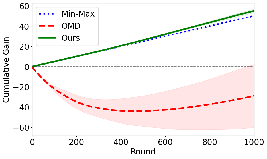
All vs RandMinMax($0.15$)

 

All vs RandMinMax($0.3$)

All vs RandMinMax($0.5$)

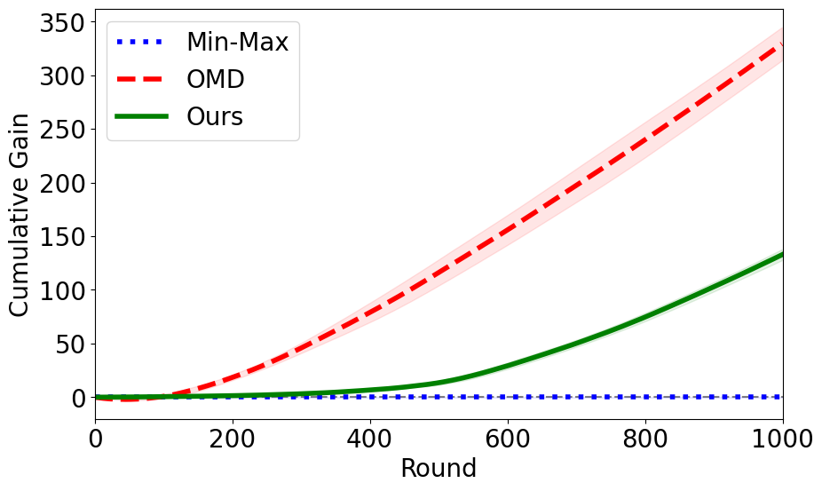
All vs RaiseK

Figure 4: All vs Bob comparison for $T=1000$ rounds. The x-axis displays the round $t$, and the y-axis displays how much Min-Max, OMD, and Algorithm˜2 gained from the second algorithm so far. The y-axes have varying scales for readability.

All vs RandMinMax($\alpha$): In all plots, our Algorithm˜2 achieves at least the gain of the min-max equilibrium and in fact always improves slightly over it. For small values of $\alpha$ (e.g. $\alpha=0.05$), meaning that Bob plays a (reasonable) strategy very close to the min-max equilibrium, OMD always loses money while Algorithm˜2 wins linearly. For larger values of $\alpha$ (e.g. $\alpha=0.1,0.15,0.3$), OMD loses an initial amount but slowly starts catching up towards a total positive gain for very large $T$. Finally, when $\alpha$ is large (e,g, $\alpha=0.5$), meaning that Bob plays a highly suboptimal (and not exploitative) strategy, OMD is able to obtain a positive gain much quicker and eventually surpasses our Algorithm˜2 (as it is not restricted to the support of the min-max equilibrium, which in this case is of advantage).

All vs RaiseK: Notice that min-max equilibrium does not exploit RaiseK at all. At the same time, OMD exploits it linearly right away, extracting a near-optimal gain from the opponent. Our Algorithm˜2 also exploits RaiseK linearly at a comparable slope, however starting exploitation somewhat delayed due to the risk-averse nature of the algorithm. However, our algorithm consistently exploits weak opponents significantly better than the min-max strategy in all cases, and unlike OMD does so while not risking to lose essentially any money.

In summary, our experimental evaluations reveal the following insights that are in accordance with our theoretical findings: If Alice plays Algorithm˜2, she secures at least the gain of the min-max strategy, thus not losing against any opponent. Yet, she is able to better exploit strategies that deviate from the min-max strategy, at a level often comparable to standard no-regret algorithms.

Implementation Details. In all experiments, we average $n=5$ runs of repeated play (plotting Alice’s average cumulative expected gain), and plot one standard deviation. In all algorithms, we used the same learning fixed rates ($\eta\sim 1/\sqrt{T}$) and the (unbalanced) dilated KL divergence for fairness and simplicity. All simulations were performed on a MacBook Pro 2.8 GHz Quad-Core Intel Core i7. We provide the code in the supplementary material.

References

- Ananthakrishnan et al. (2024) Nivasini Ananthakrishnan, Nika Haghtalab, Chara Podimata, and Kunhe Yang. Is knowledge power? on the (im) possibility of learning from strategic interaction. arXiv preprint arXiv:2408.08272, 2024.
- Arunachaleswaran et al. (2024) Eshwar Ram Arunachaleswaran, Natalie Collina, and Jon Schneider. Pareto-optimal algorithms for learning in games. In Proceedings of the 25th ACM Conference on Economics and Computation, pages 490–510, 2024.
- Auer et al. (1995) Peter Auer, Nicolo Cesa-Bianchi, Yoav Freund, and Robert E Schapire. Gambling in a rigged casino: The adversarial multi-armed bandit problem. In Proceedings of IEEE 36th annual foundations of computer science, pages 322–331. IEEE, 1995.
- Auer et al. (2008) Peter Auer, Thomas Jaksch, and Ronald Ortner. Near-optimal regret bounds for reinforcement learning. Advances in neural information processing systems, 21, 2008.
- Badanidiyuru et al. (2018) Ashwinkumar Badanidiyuru, Robert Kleinberg, and Aleksandrs Slivkins. Bandits with knapsacks. Journal of the ACM (JACM), 65(3):1–55, 2018.
- Bai et al. (2022) Yu Bai, Chi Jin, Song Mei, and Tiancheng Yu. Near-optimal learning of extensive-form games with imperfect information. In International Conference on Machine Learning, pages 1337–1382. PMLR, 2022.
- Bernasconi et al. (2022) Martino Bernasconi, Federico Cacciamani, Matteo Castiglioni, Alberto Marchesi, Nicola Gatti, and Francesco Trovò. Safe learning in tree-form sequential decision making: Handling hard and soft constraints. In International Conference on Machine Learning, pages 1854–1873. PMLR, 2022.
- Bernasconi-de Luca et al. (2021) Martino Bernasconi-de Luca, Federico Cacciamani, Simone Fioravanti, Nicola Gatti, Alberto Marchesi, and Francesco Trovò. Exploiting opponents under utility constraints in sequential games. Advances in Neural Information Processing Systems, 34:13177–13188, 2021.
- Braggion et al. (2020) Eleonora Braggion, Nicola Gatti, Roberto Lucchetti, Tuomas Sandholm, and Bernhard Von Stengel. Strong nash equilibria and mixed strategies. International Journal of Game Theory, 49:699–710, 2020.
- Brown et al. (2023) William Brown, Jon Schneider, and Kiran Vodrahalli. Is learning in games good for the learners? In Thirty-seventh Conference on Neural Information Processing Systems, 2023. URL https://openreview.net/forum?id=jR2FkqW6GB.
- Cai et al. (2023) Linda Cai, S Matthew Weinberg, Evan Wildenhain, and Shirley Zhang. Selling to multiple no-regret buyers. In International Conference on Web and Internet Economics, pages 113–129. Springer, 2023.
- Cesa-Bianchi and Lugosi (2006) Nicolo Cesa-Bianchi and Gábor Lugosi. Prediction, learning, and games. Cambridge university press, 2006.
- Chen and Lin (2023) Yiling Chen and Tao Lin. Persuading a behavioral agent: Approximately best responding and learning. arXiv preprint arXiv:2302.03719, 2023.
- Cutkosky and Orabona (2018) Ashok Cutkosky and Francesco Orabona. Black-box reductions for parameter-free online learning in banach spaces. In Conference On Learning Theory, pages 1493–1529. PMLR, 2018.
- Damer and Gini (2017) Steven Damer and Maria Gini. Safely using predictions in general-sum normal form games. In Proceedings of the 16th conference on autonomous agents and multiagent systems, pages 924–932, 2017.
- Deng et al. (2019) Yuan Deng, Jon Schneider, and Balasubramanian Sivan. Strategizing against no-regret learners. Advances in Neural Information Processing Systems, 32, 2019.
- Efroni et al. (2020) Yonathan Efroni, Shie Mannor, and Matteo Pirotta. Exploration-exploitation in constrained mdps. arXiv preprint arXiv:2003.02189, 2020.
- Even-Dar et al. (2008) Eyal Even-Dar, Michael Kearns, Yishay Mansour, and Jennifer Wortman. Regret to the best vs. regret to the average. Machine Learning, 72(1):21–37, 2008.
- Fan et al. (2024) Zhiyuan Fan, Christian Kroer, and Gabriele Farina. On the optimality of dilated entropy and lower bounds for online learning in extensive-form games. arXiv preprint arXiv:2410.23398, 2024.
- Farina et al. (2019) Gabriele Farina, Christian Kroer, and Tuomas Sandholm. Online convex optimization for sequential decision processes and extensive-form games. In AAAI Conference on Artificial Intelligence, 2019.
- Farina et al. (2021) Gabriele Farina, Robin Schmucker, and Tuomas Sandholm. Bandit linear optimization for sequential decision making and extensive-form games. In AAAI Conference on Artificial Intelligence, 2021.
- Fiegel et al. (2023a) Côme Fiegel, Pierre Ménard, Tadashi Kozuno, Rémi Munos, Vianney Perchet, and Michal Valko. Adapting to game trees in zero-sum imperfect information games. In International Conference on Machine Learning, pages 10093–10135. PMLR, 2023a.
- Fiegel et al. (2023b) Côme Fiegel, Pierre Ménard, Tadashi Kozuno, Rémi Munos, Vianney Perchet, and Michal Valko. Local and adaptive mirror descents in extensive-form games. arXiv preprint arXiv:2309.00656, 2023b.
- Ganzfried and Sandholm (2015) Sam Ganzfried and Tuomas Sandholm. Safe opponent exploitation. ACM Transactions on Economics and Computation (TEAC), 3(2):1–28, 2015.
- Ganzfried and Sun (2018) Sam Ganzfried and Qingyun Sun. Bayesian opponent exploitation in imperfect-information games. In 2018 IEEE Conference on Computational Intelligence and Games (CIG), pages 1–8. IEEE, 2018.
- Garcelon et al. (2020) Evrard Garcelon, Mohammad Ghavamzadeh, Alessandro Lazaric, and Matteo Pirotta. Conservative exploration in reinforcement learning. In International conference on artificial intelligence and statistics, pages 1431–1441. PMLR, 2020.
- Ge et al. (2024) Zhenxing Ge, Zheng Xu, Tianyu Ding, Linjian Meng, Bo An, Wenbin Li, and Yang Gao. Safe and robust subgame exploitation in imperfect information games. In Forty-first International Conference on Machine Learning, 2024.
- Guruganesh et al. (2024) Guru Guruganesh, Yoav Kolumbus, Jon Schneider, Inbal Talgam-Cohen, Emmanouil-Vasileios Vlatakis-Gkaragkounis, Joshua R Wang, and S Matthew Weinberg. Contracting with a learning agent. arXiv preprint arXiv:2401.16198, 2024.
- Haghtalab et al. (2024) Nika Haghtalab, Chara Podimata, and Kunhe Yang. Calibrated stackelberg games: Learning optimal commitments against calibrated agents. Advances in Neural Information Processing Systems, 36, 2024.
- Hazan (2019) Elad Hazan. Introduction to online convex optimization. CoRR, abs/1909.05207, 2019. URL http://arxiv.org/abs/1909.05207.
- Hoda et al. (2010) Samid Hoda, Andrew Gilpin, Javier Peña, and Tuomas Sandholm. Smoothing techniques for computing nash equilibria of sequential games. Math. Oper. Res., 35(2):494–512, 2010.
- Hutter et al. (2005) Marcus Hutter, Jan Poland, and Manfred Warmuth. Adaptive online prediction by following the perturbed leader. Journal of Machine Learning Research, 6(4), 2005.
- Jakobsen et al. (2016) Sune K Jakobsen, Troels B Sørensen, and Vincent Conitzer. Timeability of extensive-form games. In Proceedings of the 2016 ACM Conference on Innovations in Theoretical Computer Science, pages 191–199, 2016.
- Kapralov and Panigrahy (2011) Michael Kapralov and Rina Panigrahy. Prediction strategies without loss. Advances in Neural Information Processing Systems, 24, 2011.
- Kolumbus and Nisan (2022a) Yoav Kolumbus and Noam Nisan. How and why to manipulate your own agent: On the incentives of users of learning agents. Advances in Neural Information Processing Systems, 35:28080–28094, 2022a.
- Kolumbus and Nisan (2022b) Yoav Kolumbus and Noam Nisan. Auctions between regret-minimizing agents. In Proceedings of the ACM Web Conference 2022, pages 100–111, 2022b.
- Koolen (2013) Wouter M Koolen. The pareto regret frontier. Advances in Neural Information Processing Systems, 26, 2013.
- Kozuno et al. (2021) Tadashi Kozuno, Pierre Ménard, Rémi Munos, and Michal Valko. Model-free learning for two-player zero-sum partially observable markov games with perfect recall. arXiv preprint arXiv:2106.06279, 2021.
- Kuhn (1950) Harold W Kuhn. A simplified two-person poker. Contributions to the Theory of Games, 1(97-103):2, 1950.
- Lanctot et al. (2009) Marc Lanctot, Kevin Waugh, Martin Zinkevich, and Michael Bowling. Monte carlo sampling for regret minimization in extensive games. Advances in neural information processing systems, 22, 2009.
- Lattimore (2015) Tor Lattimore. The pareto regret frontier for bandits. Advances in Neural Information Processing Systems, 28, 2015.
- Lattimore and Szepesvári (2020) Tor Lattimore and Csaba Szepesvári. Bandit algorithms. Cambridge University Press, 2020.
- Liu et al. (2022) Mingyang Liu, Chengjie Wu, Qihan Liu, Yansen Jing, Jun Yang, Pingzhong Tang, and Chongjie Zhang. Safe opponent-exploitation subgame refinement. Advances in Neural Information Processing Systems, 35:27610–27622, 2022.
- Liu et al. (2021) Tao Liu, Ruida Zhou, Dileep Kalathil, Panganamala Kumar, and Chao Tian. Learning policies with zero or bounded constraint violation for constrained mdps. Advances in Neural Information Processing Systems, 34:17183–17193, 2021.
- Maiti et al. (2023) Arnab Maiti, Kevin Jamieson, and Lillian J Ratliff. Logarithmic regret for matrix games against an adversary with noisy bandit feedback. arXiv preprint arXiv:2306.13233, 2023.
- Mansour et al. (2022) Yishay Mansour, Mehryar Mohri, Jon Schneider, and Balasubramanian Sivan. Strategizing against learners in bayesian games. In Conference on Learning Theory, pages 5221–5252. PMLR, 2022.
- Orabona (2019) Francesco Orabona. A modern introduction to online learning. arXiv preprint arXiv:1912.13213, 2019.
- Orabona and Pál (2016) Francesco Orabona and Dávid Pál. Coin betting and parameter-free online learning. Advances in Neural Information Processing Systems, 29, 2016.
- Osborne and Rubinstein (1994) Martin J Osborne and Ariel Rubinstein. A course in game theory. MIT Press, 1994.
- Ponsen et al. (2011) Marc J. V. Ponsen, Steven de Jong, and Marc Lanctot. Computing approximate nash equilibria and robust best-responses using sampling. J. Artif. Intell. Res., 42:575–605, 2011. URL https://api.semanticscholar.org/CorpusID:6347533.
- Sani et al. (2014) Amir Sani, Gergely Neu, and Alessandro Lazaric. Exploiting easy data in online optimization. Advances in Neural Information Processing Systems, 27, 2014.
- van der Hoeven et al. (2020) Dirk van der Hoeven, Ashok Cutkosky, and Haipeng Luo. Comparator-adaptive convex bandits. Advances in Neural Information Processing Systems, 33:19795–19804, 2020.
- Von Neumann and Morgenstern (2007) John Von Neumann and Oskar Morgenstern. Theory of games and economic behavior: 60th anniversary commemorative edition. In Theory of games and economic behavior. Princeton university press, 2007.
- Wu et al. (2016) Yifan Wu, Roshan Shariff, Tor Lattimore, and Csaba Szepesvári. Conservative bandits. In International Conference on Machine Learning, pages 1254–1262. PMLR, 2016.
- Zhang and Sandholm (2021) Brian Zhang and Tuomas Sandholm. Subgame solving without common knowledge. Advances in Neural Information Processing Systems, 34:23993–24004, 2021.
- Zinkevich et al. (2007) Martin Zinkevich, Michael Johanson, Michael Bowling, and Carmelo Piccione. Regret minimization in games with incomplete information. Advances in neural information processing systems, 20, 2007.