Exact Upper and Lower Bounds for the Output Distribution
of Neural Networks with Random Inputs

Abstract

We derive exact upper and lower bounds for the cumulative distribution function (cdf) of the output of a neural network over its entire support subject to noisy (stochastic) inputs. The upper and lower bounds converge to the true cdf over its domain as the resolution increases. Our method applies to any feedforward NN using continuous monotonic piecewise differentiable activation functions (e.g., ReLU, tanh and softmax) and convolutional NNs, which were beyond the scope of competing approaches. The novelty and an instrumental tool of our approach is to bound general NNs with ReLU NNs. The ReLU NN based bounds are then used to derive upper and lower bounds of the cdf of the NN output. Experiments demonstrate that our method delivers guaranteed bounds of the predictive output distribution over its support, thus providing exact error guarantees, in contrast to competing approaches.

1 Introduction

Increased computational power, availability of large datasets, and the rapid development of new NN architectures contribute to the ongoing success of neural network (NN) based learning in image recognition, natural language processing, speech recognition, robotics, strategic games, etc. A limitation of NN machine learning (ML) approaches is that it is difficult to infer the uncertainty of the predictions from their results: there is no internal mechanism in NN learning to assess how trustworthy the network outputs are with not seen data. A NN is a model of the form:

$$Y =f(X,{\bm{\Theta}}),$$ (1)

where $Y$ is the output and $X$ the input (typically multivariate), and $f$ is a known function modeling the relationship between $X$ and $Y$ parametrized by $\Theta$. Model (1) incorporates uncertainty neither in $Y$ nor in $X$ and NN fitting is a numerical algorithm for minimizing a loss function. Lack of uncertainty quantification, such as assessment mechanisms for prediction accuracy beyond the training data, prevents neural networks, despite their potential, from being deployed in safety-critical applications ranging from medical diagnostic systems (e.g., (Hafiz & Bhat, 2020)) to cyber-physical systems such as autonomous vehicles, robots or drones (e.g., (Yurtsever et al., 2020)). Also, the deterministic nature of NNs renders them highly vulnerable to not only adversarial noise but also to even small perturbations in inputs ((Bibi et al., 2018; Fawzi et al., 2018; Goodfellow et al., 2014a, b; Hosseini et al., 2017)).

Uncertainty in modeling is typically classified as epistemic or systematic, which derives from lack of knowledge of the model, and aleatoric or statistical, which reflects the inherent randomness in the underlying process being modeled (see, e.g., (Hüllermeier & Waegeman, 2021)). The universal approximation theorem (UAT) (Cybenko, 1989; Hornik et al., 1989) states that a neural network with one hidden layer can approximate any continuous function for inputs within a specific range by increasing the number of neurons. In the context of NNs, epistemic uncertainty is of secondary importance to aleatoric uncertainty. Herein, we focus on studying the effect of random inputs on the output distribution of NNs and derive uniform upper and lower bounds for the cumulative distribution function (cdf) of the outputs of a NN subject to noisy (stochastic) input data.

We evaluate our proposed framework on three benchmark datasets (Iris (Fisher, 1936), Wine (Aeberhard & Forina, 1992) and Diabetes (Efron et al., 2004)) and demonstrate the efficacy of our approach to bound the cdf of the NN output subject to Gaussian and Gaussian mixture inputs. We demonstrate that our bounds cover the true underlying cdf over its entire support. In contrast, the directly competing approach of Krapf et al. (2024), as well as high-sample Monte-Carlo simulations, produce estimates outside the bounds over several areas of the output range.

2 Statement of the Problem

A neural network is a mathematical model that produces outputs from inputs. The input is typically a vector of predictor variables, ${\mathbf{X}}\in^{n_{0}}$, and the output $Y$, is univariate or multivariate, continuous or categorical.

A feedforward NN with $L$ layers from ${}^{n_{0}}\to^{n_{L}}$ is a composition of $L$ functions,

$$f_{L}({\mathbf{x}};{\bm{\Theta}}) =f^{(L)}\circ f^{(L-1)}\circ...\circ f^{(1)}({\mathbf{x}}),$$ (2)

where the $l$-th layer is given by

$$f^{(l)}({\mathbf{x}};{\mathbf{W}}^{(l)},{\mathbf{b}}^{(l)})=\sigma^{(l)}({\mathbf{W}}^{(l)}{\mathbf{x}}+{\mathbf{b}}^{(l)}),$$

with weights ${\mathbf{W}}^{(l)}\in\mathbb{R}^{n_{l}\times n_{l-1}}$, bias terms ${\mathbf{b}}^{(l)}\in\mathbb{R}^{n_{l}}$, and a non-constant, continuous activation function $\sigma^{(l)}:\to$ that is applied component-wise. The NN parameters are collected in ${\bm{\Theta}}=(\text{vec}({\mathbf{W}}_{1})$, ${\mathbf{b}}_{1},\ldots$, $\text{vec}({\mathbf{W}}_{L})$, ${\mathbf{b}}_{L})\in^{\sum_{l=1}^{L}(n_{l-1}\cdot n_{l}+n_{l})}$. The first layer that receives the input ${\mathbf{x}}$ is called the input layer, and the last layer is the output layer. All other layers are called hidden. For categorical outputs, the class label is assigned by a final application of a decision function, such as $\mathrm{arg\,max}$.

Despite not being typically acknowledged, the training data in NNs are drawn from larger populations, and hence they contain only limited information about the corresponding population. We incorporate the uncertainty associated with the observed data assuming that they are random draws from an unknown distribution of bounded support. That is, the data are comprised of $m$ draws from the joint distribution of $({\mathbf{X}},Y)$, and the network is trained on observed $({\mathbf{x}}_{i},y_{i})$, ${\mathbf{x}}_{i}=(x_{i1},x_{i2},\ldots,x_{in_{0}})$, and $y_{i}$, $i=1,\ldots,$$m$. A NN with $L$ layers and $n_{l}$ neurons at each layer, $l=1,\ldots,L$, is trained on the observed $({\mathbf{x}}_{i},y_{i})$, $i=1,\ldots,m$, to produce $m$ outputs $\tilde{y}_{i}$, and the vector of the NN parameters, ${\bm{\Theta}}=\left(\operatorname{vec}({\mathbf{W}}_{1}),{\mathbf{b}}_{1},\ldots,\operatorname{vec}({\mathbf{W}}_{L}),{\mathbf{b}}_{L}\right)$, is obtained. ${\bm{\Theta}}$ uniquely identifies the trained NN. Given ${\bm{\Theta}}$, we aim to quantify the robustness of the corresponding NN, to perturbations in the input variables. For this, we let

$${\mathbf{X}}\sim F_{{\mathbf{X}}},$$ (3)

where ${\mathbf{X}}\in^{n_{0}}$ stands for the randomly perturbed input variables with cdf $F_{{\mathbf{X}}}$ and probability density function (pdf) $\phi({\mathbf{x}})$ that is piecewise continuous and bounded on a compact support. We study the propagation of uncertainty (effect of the random perturbation) in the NN by deriving upper and lower bounds of the cdf $F_{{\widetilde{\mathbf{Y}}}}(y)=\mathbb{P}({\widetilde{\mathbf{Y}}}\leq y)$ of the random output, ${\widetilde{\mathbf{Y}}}=f_{L}({\mathbf{X}}\mid{\bm{\Theta}})$.

Our contributions:

1. We develop a method to compute the exact cdf of the output of ReLU NNs with random input pdf, which is a piecewise polynomial over a compact hyperrectangle. This result, which can be viewed as a stochastic analog to the Stone-Weierstrass theorem, significantly contributes to the characterization of the distribution of the output of NNs with piecewise-linear activation functions under any input continuous pdf.

2. We derive guaranteed upper and lower bounds of the NN output distribution resulting from random input perturbations on a fixed support. This provides exact upper and lower bounds for the output cdf provided the input values fall within the specified support. No prior knowledge about the true cdf is required to guarantee the validity of our bounds.

3. We show the convergence of our bounds to the true cdf; that is, our bounds can be refined to arbitrary accuracy.

4. We provide a constructive proof that any feedforward NN with continuous monotonic piecewise differentiable activation functions can be both upper and lower approximated by a fully connected ReLU network, achieving any desired level of accuracy. Moreover, we enable the incorporation of multivariate operations such as $\max$, $\mathrm{product}$ and $\mathrm{softmax}$, as well as some non-monotonic functions such as $|x|$ and $x^{n},n\in{\mathbb{N}}$.

5. We prove a new universal distribution approximation theorem (UDAT), which states that we can estimate the cdf of the output of any continuous function of a random variable (or vector) that has a continuous distribution supported on a compact hyperrectangle, achieving any desired level of accuracy.

3 Our Approximation Approach

We aim to estimate the cdf $F_{{\widetilde{\mathbf{Y}}}}(y)$ of the output ${\widetilde{\mathbf{Y}}}=f_{L}({\mathbf{X}}\mid{\bm{\Theta}})$ of the NN in (2) under (3); i.e., subject to random perturbations of the input ${\mathbf{X}}$. We do so by computing upper and lower bounds of $F_{{\widetilde{\mathbf{Y}}}}$; that is, we compute $\overline{F}_{{\widetilde{\mathbf{Y}}}}$, $\underline{F}_{{\widetilde{\mathbf{Y}}}}$ such that

$$\underline{F}_{{\widetilde{\mathbf{Y}}}}(y)\leq F_{{\widetilde{\mathbf{Y}}}}(y)\leq\overline{F}_{{\widetilde{\mathbf{Y}}}}(y),\,\forall y$$ (4)

We refer to the NN in (2) as prediction NN when needed for clarity. We estimate the functions $\overline{F}_{{\widetilde{\mathbf{Y}}}}$, $\underline{F}_{{\widetilde{\mathbf{Y}}}}$ on a “superset” of the output domain of the prediction NN (2) via an integration procedure. The cdf of ${\widetilde{\mathbf{Y}}}$ is given by

$$F_{{\widetilde{\mathbf{Y}}}}(y) =\mathbb{P}({\widetilde{\mathbf{Y}}}\leq y)=\int_{\{{\widetilde{\mathbf{Y}}}\leq y\}}\phi({\mathbf{x}})d{\mathbf{x}},$$ (5)

where $\phi({\mathbf{x}})$ is the pdf of ${\mathbf{X}}$. To bound $F_{{\widetilde{\mathbf{Y}}}}$, we bound $\phi$ by its upper ($\overline{\phi}$) and lower ($\underline{\phi}$) estimates on the bounded support of $\phi$ as described in Section 3.3. If $\phi$ is a piecewise polynomial, then 5 can be computed exactly for a ReLU prediction network, as we show in Section 3.1. Once $\overline{\phi}$, $\underline{\phi}$ are estimated, then

$$\underline{F}_{\widetilde{Y}}(y)= \int_{\{{\widetilde{\mathbf{Y}}}\leq y\}}\underline{\phi}({\mathbf{x}})dx\leq F_{{\widetilde{\mathbf{Y}}}}(y)\leq$$ (6)

$$\int_{\{{\widetilde{\mathbf{Y}}}\leq y\}}\overline{\phi}({\mathbf{x}})dx=\overline{F}_{{\widetilde{\mathbf{Y}}}}(y)$$

Remark 3.1.

$\underline{F}_{{\widetilde{\mathbf{Y}}}}(y)$ and $\overline{F}_{{\widetilde{\mathbf{Y}}}}(y)$ are not always true cdfs since we allow the lower estimator not to achieve 1, while the upper bound is allowed to take the smallest value greater than 0.

3.1 Exact cdf evaluation for a fully connected NN with ReLU activation function

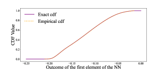
Figure 1: Exact CDF of the ReLU neural network outcome for the class Setosa in the Iris problem, assuming Beta-distributed inputs.

Definition 3.2 (Almost disjoint sets).

We say that sets $\mathcal{A}$ and $\mathcal{B}$ are almost disjoint with respect to measure $\alpha$, if $\alpha(\mathcal{A}\cap\mathcal{B})=0$.

Definition 3.3 (Closed halfspace).

A $n_{0}$-dimensional closed halfspace is a set $H=\{x\in^{n_{0}}|{\mathbf{v}}^{T}x\leq c\}$ for $c\in$ and some ${\mathbf{v}}\in^{n_{0}}$, which is called the normal of the halfspace.

It is known that a convex polytope can be represented as an intersection of halfspaces, called $\mathcal{H}$-representation (Ziegler (1995)).

Definition 3.4 ($\mathcal{H}$-polytope).

A $n_{0}$-dimensional $\mathcal{H}$-polytope $\mathcal{C}=\bigcap\limits_{j=1}^{h}H_{i}$ is the intersection of finitely many closed halfspaces.

Definition 3.5 (Simplex).

A $n_{0}$-dimensional simplex is a $n_{0}$-dimensional polytope with $n_{0}+1$ vertices.

Definition 3.6 (Piecewise polynomial).

A function $p:K\rightarrow^{n_{L}}$ is a piecewise polynomial, if there exists a finite set of $n_{0}$-simplices such that $K=\bigcup\limits_{i=1}^{q}k_{i}$ and the function $p$ constrained to the interior ${\kern 0.0ptk}^{\mathrm{o}}_{i}$ of $k_{i}$ is a polynomial; that is, $p\big{|}_{{\kern 0.0ptk}^{\mathrm{o}}_{i}}:{\kern 0.0ptk}^{\mathrm{o}}_{i}\rightarrow^{n_{L}}$ is a polynomial for all $i=1,\ldots,q$.

Remark 3.7.

We do not require piecewise polynomials to be continuous everywhere on the hyperrectangle. Specifically, we allow discontinuities at the borders of simplices. However, the existence of left and right limits of the function at every point on the bounded support is guaranteed by the properties of standard polynomials.

Raghu et al. (2017) showed that ReLU deep networks divide the input domain into activation patterns (see Sudjianto et al. (2020)) that are disjoint convex polytopes $\{\mathcal{C}_{j}\}$ over which the output function is locally represented as the affine transformation $f_{L}({\mathbf{x}})=NN^{j}({\mathbf{x}})=\mathbf{c}^{j}+{\mathbf{V}}^{j}{\mathbf{x}}$ for ${\mathbf{x}}\in\{\mathcal{C}_{j}\}$, the number of which grows at the order $\mathcal{O}((\max\{n_{l}\}_{l=1,\ldots,L})^{n_{0}L})$. Sudjianto et al. (2020) outline an algorithm for extracting the full set of polytopes and determining local affine transformations, including the coefficients $\mathbf{c}^{j},{\mathbf{V}}^{j}$ for all $\{\mathcal{C}_{j}\}$, by propagating through the layers. For our computations, we utilize a recent GPU-accelerated algorithm from Berzins (2023).

We aim to derive a superset of the range of the network output. For this, we exploit the technique of Interval Bound Propagation (IBP), based on ideas from (Gowal et al., 2018; Wang et al., 2022; Gehr et al., 2018). Propagating the $n_{0}$-dimensional box through the network leads to the superset of the range of the network output. We compute the cdf of the network’s output at each point of a grid of the superset of the output range.

Theorem 3.8 (Exact cdf of ReLU NN w.r.t. piecewise polynomial pdf).

Let ${\widetilde{\mathbf{Y}}}:^{n_{0}}\rightarrow^{n_{L}}$ be a feed-forward ReLU neural network, which splits the input space into a set of almost disjoint polytopes $\{\mathcal{C}_{j}\}_{j=1}^{q_{Y}}$ with local affine transformations ${\widetilde{\mathbf{Y}}}({\mathbf{x}})=NN^{j}({\mathbf{x}})$ for ${\mathbf{x}}\in\mathcal{C}_{j}$. Let $\phi({\mathbf{x}})$ denote the pdf of the random vector ${\mathbf{X}}$ that is a piecewise polynomial with local polynomials, $\phi({\mathbf{x}})=\phi_{i}({\mathbf{x}})$ for all ${\mathbf{x}}\in{\kern 0.0ptk}^{\mathrm{o}}_{i}$ over an almost disjoint set of simplices $\{k_{i}\}_{i=1}^{q_{\phi}}$, and a compact hyperrectangle support $K\subset^{n_{0}}$. Then, the cdf of ${\widetilde{\mathbf{Y}}}$ is

$$F_{{\widetilde{\mathbf{Y}}}}({\mathbf{y}})=\mathbb{P}\left[{\widetilde{\mathbf{Y}}}\leq{\mathbf{y}}\right] =\sum\limits_{i=1}^{q_{\phi}}\sum\limits_{j=1}^{q_{Y}}\mathcal{I}\left[\phi_{i}({\mathbf{x}});\mathcal{C}^{r}_{j,i}\right]$$

$$=\sum\limits_{i=1}^{q_{\phi}}\sum\limits_{j=1}^{q_{Y}}\sum\limits_{s=1}^{S_{i,j}}\mathcal{I}\left[\phi_{i}({\mathbf{x}});\mathcal{T}_{i,j,s}\right],$$

where $\mathcal{I}\left[\phi_{i}({\mathbf{x}});\mathcal{T}_{i,j,s}\right]$ is the integral of the local polynomial $\phi_{i}({\mathbf{x}})$ over the simplex $\mathcal{T}_{i,j,s}$ such that the reduced polytope

$$\mathcal{C}^{r}_{j,i}=\mathcal{C}_{j}\cap k_{i}\cap\{{\mathbf{x}}:NN^{j}({\mathbf{x}})\leq{\mathbf{y}}\}=\bigcup\limits_{s=1}^{S_{i,j}}\mathcal{T}_{i,j,s}$$ (7)

is defined by the intersection of polytopes $\mathcal{C}_{j}$ and $k_{i}$, and an intersection of halfspaces

$$\{{\mathbf{x}}:NN^{j}({\mathbf{x}})\leq{\mathbf{y}}\}=\bigcap\limits_{t=1}^{n_{L}}\left\{{\mathbf{x}}:NN^{j}_{t}({\mathbf{x}})\leq y_{t}\right\}.$$

Theorem 3.8 is shown in Appendix A.1. The proof relies on the algorithm for evaluating the integral of a polynomial over a simplex as described in Lasserre (2021). The right-hand side of (7) results from the Delaunay triangulation, dividing the reduced polytope $\mathcal{C}^{r}_{j,i}$ into $S_{i,j}$ almost disjoint simplices.

Remark 3.9.

Theorem 3.8 is a tool for approximating the output cdf of any feedforward neural network with piecewise linear activation functions on a compact domain, given random inputs with arbitrary continuous distribution at any desired degree of accuracy (see 4).

Example 3.10.

We compute the output cdf of a 3-layer, 12-neuron fully connected ReLU neural network with the last (before $\mathrm{softmax}$) linear 3-neuron layer trained on the Iris dataset (Fisher, 1936). The Iris dataset consists of 150 samples of iris flowers from three different species: Setosa, Versicolor, and Virginica. Each sample includes four features: Sepal Length, Sepal Width, Petal length, and Petal width. We focused on two features, Sepal Length and Sepal Width (scaled to $[0,1]$), classifying objects into three classes. Specifically, we recovered the distribution of the first component (class Setosa) before applying the $\mathrm{softmax}$ function, assuming Beta-distributed inputs with parameters $(2,2)$ and $(3,2)$. The exact cdf is plotted in purple in Figure 1, with additional details provided in Appendix C. The agreement with the empirical cdf is almost perfect.

3.2 Algorithm for Upper and Lower Approximation of the Neural Network using ReLU activation functions.

Theorem 3.11.

Let $\widetilde{Y}$ be a feedforward neural network with $L$ layers of arbitrary width with continuous non-decreasing piecewise differentiable activation functions at each node. There exist sequences of fully connected ReLU neural networks $\{\overline{Y}_{n}\}$, $\{\underline{Y}_{n}\}$ with $L$ layers, which are monotonically decreasing and increasing, respectively, such that for any $\epsilon>0$ and any compact hyperrectangle $K\subset^{n_{0}}$, one can find $N\in{\mathbb{N}}$ such that for all $n\geq N$

$$0\leq\widetilde{Y}({\mathbf{x}})-\underline{Y}_{n}({\mathbf{x}})<\epsilon,\quad 0\leq\overline{Y}_{n}({\mathbf{x}})-\widetilde{Y}({\mathbf{x}})<\epsilon$$

for all ${\mathbf{x}}\in K$.

We develop an approach to approximate a neural network’s activation functions and, consequently, the output of the neural network, using the ReLU activation function to create piecewise linear upper and lower bounds. These bounds approximate the true activation function, allowing a more analyzable neural network. This method is a constructive proof of Theorem 3.11 and applies to any fully connected or convolution (CNN) feedforward neural network with non-decreasing continuous piecewise differentiable activation functions that is analyzed on a hyperrectangle. The key features of our approach are:

• Local adaptability: The algorithm adapts to the curvature of the activation function, providing an adaptive approximation scheme depending on whether the function is locally convex or concave.

• Streamlining: By approximating the network with piecewise linear functions, the complexity of analyzing the network output is significantly reduced.

How it works:

Input/Output range evaluation:

Using IBP (Gowal et al., 2018), we compute supersets of the input and output ranges of the activation function for every neuron and every layer.

Segment Splitting:

First, input intervals are divided into macro-areas based on inflection points (different curvature areas) and non-differentiable points (e.g., $0$ for ReLU). Next, these macro-areas are subdivided into intervals based on user-specified points or their predefined number within each range. The algorithm utilizes knowledge about the behavior of the activation function and differentiates between concave and convex regions of the activation function, which impacts how the approximations are constructed and how to choose the points of segment splitting. A user defines the number of splitting segments and the algorithm ensures the resulting disjoint sub-intervals are properly ordered and on each sub-interval the function is either concave or convex. If the function is linear in a given area, it remains unchanged, with the upper and lower approximations equal to the function itself.

Upper and Lower Approximations:

The method constructs tighter upper and lower bounds through the specific choice of points and subsequent linear interpolation. It calculates new points within each interval (one per interval) and uses them to refine the approximation, ensuring the linear segments closely follow the curvature of the activation function.

The method guarantees that the piecewise linear approximation of the activation function for each neuron (a) is a non-decreasing function, and (b) the output domain remains the same.

To see this, consider a neuron of a layer. For upper (lower) approximation on a convex (concave) segment, we choose a midpoint $a_{k^{\prime}}=(a_{k}+a_{k+1})/2$ for each subinterval $\left[a_{k},a_{k+1}\right]$ and compute a linear interpolation, as follows:

$$\kappa_{1}=\frac{f(a_{k^{\prime}})-f(a_{k})}{a_{k^{\prime}}-a_{k}},\hskip 14.22636pt\kappa_{2}=\frac{f(a_{k+1})-f(a_{k^{\prime}})}{a_{k+1}-a_{k^{\prime}}},$$

$$\widetilde{f}(\tau)=f(a_{k})+(\tau-a_{k})\kappa_{1},\hskip 12.80365pt\tau\in\left[a_{k},a_{k^{\prime}}\right]$$

$$\widetilde{f}(\tau)=f(a_{k^{\prime}})+(\tau-a_{k^{\prime}})\kappa_{2},\hskip 8.5359pt\tau\in\left[a_{k^{\prime}},a_{k+1}\right]$$

For upper (lower) approximation on a concave (convex) segment, we compute derivatives and look for tangent lines at border points of the sub-interval $\left[a_{k},a_{k+1}\right]$. We choose a point $a_{k^{\prime}}:a_{k}\leq a_{k^{\prime}}\leq a_{k+1}$ to be the intersection of the tangent lines. The original function is approximated by the following two tangent line segments:

$$a_{k^{\prime}}=\frac{f(a_{k})-f(a_{k+1})-(f_{+}^{\prime}(a_{k})a_{k}-f_{-}^{\prime}(a_{k+1})a_{k+1})}{f_{-}^{\prime}(a_{k+1})-f_{+}^{\prime}(a_{k})}$$

$$\widetilde{f}(\tau)=f(a_{k})+f_{+}^{\prime}(a_{k})(\tau-a_{k}),\hskip 32.72049pt\tau\in\left[a_{k},a_{k^{\prime}}\right]$$

$$\widetilde{f}(\tau)=f(a_{k+1})+f_{-}^{\prime}(a_{k+1})(\tau-a_{k+1}),\hskip 2.84544pt\tau\in\left[a_{k^{\prime}},a_{k+1}\right],$$

where $f_{-}^{\prime}(\cdot),f_{+}^{\prime}(\cdot)$ are left and right derivatives, respectively.

For monotonically increasing functions, this procedure guarantees that the constructed approximators are exact upper and lower approximations. Moreover, decreasing the step size (increasing the number of segments) reduces the error at each point, meaning that the sequences of approximators for the activation functions at each node are monotonic, that is $\overline{f}_{n+1}(x)\leq\overline{f}_{n}(x),\underline{f}_{n+1}(x)\geq\underline{f}_{n}(x)$ for all $x$ in the IBP domain. This procedure of piecewise linear approximation of each activation function in each neuron is equivalent to the construction of a one-layer ReLU network for a given neuron which will approximate it. By the UAT, for any continuous activation function $\sigma_{l,i}$ at each neuron and any positive $\epsilon_{l,i}$ we can always find a ReLU network-approximator $NN_{l,i}$, such that $|NN_{l,i}(x)-\sigma_{l,i}(x)|<\epsilon_{l,i}$ for all $x$ in the input domain, defined by the IBP. To find such an approximating network we need to choose the corresponding number of splitting segments of the IBP input region. Additionally, uniform convergence is preserved by Dini’s theorem, which states that a monotonic sequence of continuous functions that converges pointwise on a compact domain to a continuous function also converges uniformly. Moreover, the approximator always stays within the range of the limit function, ensuring that the domain in the next layer remains unchanged and preserves its uniform convergence.

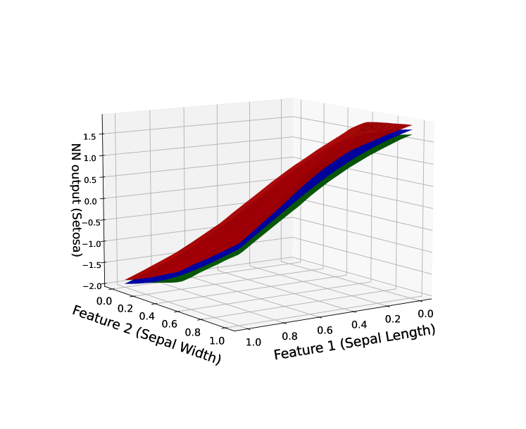
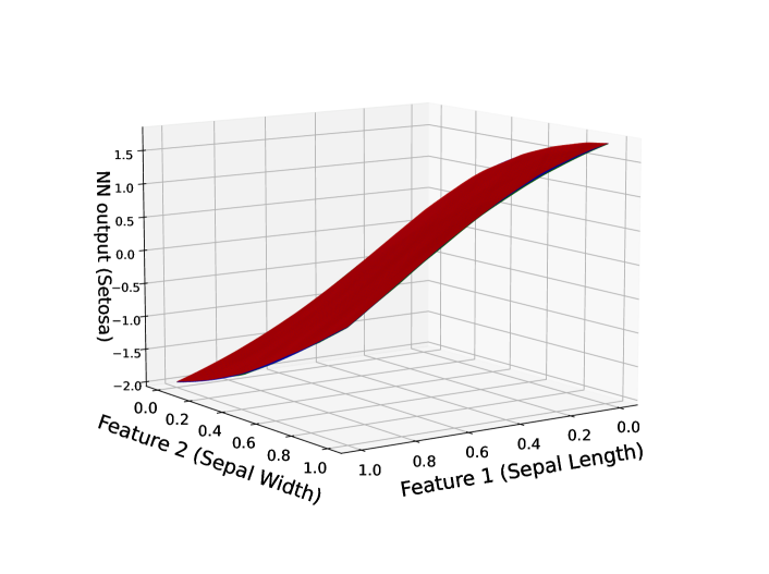
Figure 2: Tanh NN output for the Setosa class (blue) in the Iris dataset, and its ReLU NN upper (red) and lower (green) approximations with 5 (upper panel) and 10 (lower panel) segments of bounding per convex section.

Transformation into ReLU-Equivalent Form:

The approximating piecewise linear upper-lower functions are converted into a form that mimics the ReLU function’s behavior; i.e., $\tilde{f}(x)=W^{(2)}\mathrm{ReLU}(W^{(1)}x+b^{(1)})+b^{(2)}$. This involves creating new weighting coefficients and intercepts that replicate the ReLU’s activation pattern across the approximation intervals.

Specifically, we receive a set of intervals $\{\left[x_{i-1},x_{i}\right]\}_{i=1}^{n}$ with the corresponding set of parameters of affine transformations $\{\left(a_{i},b_{i}\right)\}_{i=1}^{n}$:

$$\widetilde{f}(\tau)=b_{i}+a_{i}\tau,\hskip 14.22636pt\tau\in\left[x_{i-1},x_{i}\right],$$

and additionally set $a_{0}=0$. Then, the corresponding ReLU-equivalent definition of approximation $\widetilde{f}$ on $\left[x_{0},x_{n}\right]$ is

$$\widetilde{f}(\tau)=x_{0}a_{1}+b_{1}+\sum\limits_{i=1}^{n}\xi_{i}\mathrm{ReLU}(|a_{i}-a_{i-1}|(\tau-x_{i-1})),$$

$$\xi_{i}=\operatorname{sign}(a_{i}-a_{i-1}).$$

Overall Neural Network Approximation:

The entire NN is approximated by applying the above techniques to each neuron, layer by layer, and then merging all intermediate weights and biases. For each neuron, both upper and lower approximations are generated, capturing the range of possible outputs under different inputs. To ensure the correct propagation of approximators, to create an upper approximation, we connect the upper approximation of the external layer with the upper approximation of the internal subnetwork if the internal subnetwork has a positive coefficient, or with the lower approximation if it has a negative coefficient. The reverse applies to the lower approximation. This leads to a composition of uniformly convergent sequences, guaranteeing the overall uniform convergence of the final estimator to the original neural network. The final output is a set of piecewise linear approximations that bound the output of the original neural network, which can then be used for further analysis or verification. The proof sketch is in Appendix A.2.

Example 3.12.

Using the same setup as in Example 3.10, we train a fully connected neural network with 3 layers of 12 neurons each with $\mathrm{tanh}$ activation followed by 1 layer of 3 output neurons with linear activation on the Iris dataset, focusing on the re-scaled features Sepal Length and Sepal Width. We construct upper and lower approximations of the network’s output by ReLU neural networks with linear output layer. Two approximations are performed: with 5 and 10 segments of bounding per convex section at each node (upper and lower panels of Figure 2, respectively). Notably, with 10 segments, the original network and its approximations are nearly indistinguishable.

This procedure applies to various non-monotonic functions, such as monomials $x^{n},n\in\mathbb{N}$. These functions can be attained by a sequence of transformations that ensure monotonicity at all intermediate steps. These transformations can be represented as a subnetwork. Furthermore, multivariate functions like $\mathrm{softmax}$ and the product operation also have equivalent subnetworks with continuous monotonic transformations, as shown in Appendix B.

3.3 Application to an arbitrary function on a compact domain

We present the universal distribution approximation theorem, which may serve as a starting point for further research in the field of stochastic behavior of functions and the neural networks that describe them.

Theorem 3.13 (Universal distribution approximation theorem).

Let ${\mathbf{X}}$ be a random vector with continuous pdf $\phi({\mathbf{x}})$ supported over a compact hyperrectangle $K\subset^{n_{0}}$. Let $Y=\mathcal{W}({\mathbf{x}})$ be a continuous function of ${\mathbf{X}}$ with domain $K$, and let $F(y)$ denote its cdf. Then, there exist sequences of cdf bounds $\{\underline{F}_{n}\}$, $\{\overline{F}_{n}\}$, $n=1,2,\ldots$, such that

$$\underline{F}_{n}(y)\leq F(y)\leq\overline{F}_{n}(y)$$

for all $y\in\{\mathcal{W}({\mathbf{x}}):{\mathbf{x}}\in K\}$ and

$$\underline{F}_{n}(y)\rightarrow F(y),\quad\overline{F}_{n}(y)\rightarrow F(y)$$

for all $y$ where $F(y)$ is continuous. Moreover, if $\mathcal{W}({\mathbf{X}})$ is nowhere locally constant almost surely, that is

$$\int\limits_{\{\mathcal{W}({\mathbf{x}})=y\}}\phi({\mathbf{x}})d{\mathbf{x}}=0$$ (8)

for all $y\in\{\mathcal{W}({\mathbf{x}}):{\mathbf{x}}\in K\}$, then both bounds $\underline{F}_{n},\overline{F}_{n}$ converge uniformly to the true cdf $F$. The sequence $\{\underline{F}_{n}\}$, $\{\overline{F}_{n}\}$ can be constructed by bounding the distributions of sequences of ReLU NNs.

The proof is presented in Appendix A.3. It leverages the UAT (Cybenko, 1989) to approximate the function $\mathcal{W}({\mathbf{x}})$ and input pdf $\phi({\mathbf{x}})$ with ReLU NNs to arbitrary accuracy. Cdf bounds are then computed over polytope intersections, with greater NN complexity yielding more simplices for finer local affine approximations of the pdf.

To bound the cdf of a given NN with respect to a specified input pdf, we construct upper and lower bounding ReLU NNs to approximate the target NN. Next, we subdivide the resulting polytopes of the bounding ReLU NNs into simplices as much as needed to achieve the desired accuracy and locally approximate the input pdf with constant values (the simplest polynomial form) on these simplices, transforming the problem into the one described in Section 3.1.

4 Experiments

In numerical experiments we cosider three datasets, Diabetes (Efron et al., 2004), Iris (Fisher, 1936) and, Wine (Aeberhard & Forina, 1992).

For all of the experiments, we compare our guaranteed bounds for the output cdf with cdf estimates obtained via a Monte Carlo (MC) simulation ($100$ million samples), as well as with the “Piecewise Linear Transformation” (PLT) method of Krapf et al. (2024). Given that the true cdf is contained within these limits, the experiments assess the tightness of our bounds compared to both MC and PLT by tallying the number of “out of bounds” instances. Essentially, achieving very tight bounds makes it challenging to stay within those limits, whereas even imprecise estimates can fall within broader bounds.

Our experimental setup is based on small pre-trained (fixed) neural networks. For the Diabetes dataset we trained a ReLU network with $3$ fully connected layers with $32$, $16$, and $8$ neurons, respectively. The univariate output has no activation. Training was performed on $70\%$ of the data, randomly selected. The remaining $30\%$, consisting of $73$ observations, comprise the test set. As there is no randomness in the observations, we added univariate normal noise to one randomly selected feature of every observation (different features in different observations). The standard deviation of the Gaussian noise is set to the sample standard deviation of the selected feature within the test set.

For both, Iris and Wine, we replicated the exact experimental setup from (Krapf et al., 2024) using the same test sets, Gaussian Mixtures as randomness as well as the same pre-trained networks. The $1$ to $3$ dimensional Gaussian mixtures were computed by first deleting $25\%$ or $50\%$ of the test dataset. Subsequently, $50$ new observations are imputed using MICE (van Buuren & Groothuis-Oudshoorn, 2011).The only difference in the experimental setup is the MC estimate, which we recomputed with a higher sample count. Here, the MC estimate does not play the role of the “ground truth” as in their experiments, but as another estimate.

We summarize our results in Table 1. We observe a high ratio of “out of bounds” samples for both MC and PLT compared to the number of grid points the cdf was evaluated at. This has two components: (a) In regions where the cdf is very flat, we obtain very tight bounds leading to small errors in a bucketed estimation approach easily falling outside of these tight bounds; (b) due to either pure random effect in the case of MC or numerical estimation inaccuracies in case of PLT, it produces estimates outside the bounds. We note, however, that in these examples, especially as regards PLT, a “coarse grid” can cause inaccuracies in areas where the pdf is volatile despite that their estimator targets the pdf directly and it should be more accurate than ours (as we target bounding the cdf instead).

Table 1: Comparison of our approach (guaranteed upper and lower bounds) with pointwise estimators from Monte-Carlo simulations and PLT (Krapf et al., 2024). Under column headed by $n_{0}$ are numbers of input variables, # tests gives the number of observations deleted, under U/L-dist (std) are the mean distance (standard deviation) upper and lower bounds, under $\mathrm{OOB}_{\mathrm{MC}}$ (median) and $\mathrm{OOB}_{\mathrm{PLT}}$ (median) are the average (standard deviation) of the median of number of points outside our bounds for Monte-Carlo simulations and PLT, respectively.

dataset	%unc	$n_{0}$	# tests	U/L-dist (std)	$\mathrm{OOB}_{\mathrm{MC}}$ (median)	$\mathrm{OOB}_{\mathrm{PLT}}$ (median)	Grid size
diabetes	-	1	73	0.01337 (0.005)	7 (7)	18 (19)	20
		1	25	0.00988 (0.016)	1093 (1080)	1604 (2148)	8000
iris	25	2	10	0.01236 (0.021)	793 (697)	1528 (2162)	8000
		3	–	—	—	—	8000
		1	20	0.05534 (0.077)	305 (30)	500 (4)	8000
iris	50	2	23	0.04709 (0.090)	980 (1016)	1312 (2031)	8000
		3	8	0.06864 (0.108)	779 (599)	1150 (1000)	8000
		1	32	0.02014 (0.055)	1066 (1242)	1708 (2172)	8000
wine	25	2	8	0.00909 (0.017)	1188 (1347)	1839 (2275)	8000
		3	2	0.00008 (0.000)	1324 (1324)	2516 (2516)	8000
		1	27	0.07590 (0.109)	757 (273)	1027 (45)	8000
wine	50	2	21	0.04214 (0.079)	1031 (1193)	1304 (2057)	8000
		3	13	0.06612 (0.102)	550 (128)	797 (40)	8000

5 Related Work

The literature on NN verification is not directly related to ours as it has been devoted to standard non-stochastic input NNs, where the focus is on establishing guarantees of local robustness. This line of work develops testing algorithms for whether the output of a NN stays the same within a specified neighborhood of the deterministic input (see, e.g., Gowal et al. (2018); Xu et al. (2020); Zhang et al. (2018, 2020); Shi et al. (2024); Bunel et al. (2019); Ferrari et al. (2022); Katz et al. (2017, 2019); Wu et al. (2024a)).

To handle noisy data or aleatoric uncertainty (random input) in NNs, two main approaches have been proposed: sampling-based and probability density function (pdf) approximation-based. Sampling-based methods use Monte Carlo simulations to propagate random samples through the NN (see, e.g., Abdelaziz et al. (2015); Ji et al. (2020)), but the required replications to achieve similar accuracy to theoretical approaches such as ours, as can be seen in Table 1, can be massive. Pdf approximation-based methods assume specific distributions for inputs or hidden layers, such as Gaussian (Abdelaziz et al., 2015) or Gaussian Mixture Models (Zhang & Shin, 2021), but these methods often suffer from significant approximation errors and fail to accurately quantify predictive uncertainty. Comprehensive summaries and reviews of these approaches can be found in sources like Sicking et al. (2022) and Gawlikowski et al. (2023).

In the context of verifying neural network properties within a probabilistic framework, (Weng et al., 2019) proposed PROVEN, a general probabilistic framework that ensures robustness certificates for neural networks under Gaussian and Sub-Gaussian input perturbations with bounded support with a given probability. It employs CROWN (Zhang et al., 2018, 2020) to compute deterministic affine bounds and subsequently leverages straightforward probabilistic techniques based on Hoeffding’s inequality (Hoeffding, 1963). PROVEN provides a probabilistically sound solution to ensuring the output of a NN is the same for small input perturbations with a given probability, its effectiveness hinges on the activation functions used. It cannot refine bounds or handle various input distributions, which may limit its ability to capture all adversarial attacks or perturbations in practical scenarios.

The most relevant published work to ours we could find in the literature is Krapf et al. (2024). They propagate input densities through NNs with piecewise linear activations like ReLU, without needing sampling or specific assumptions beyond bounded support. Their method calculates the propagated pdf in the output space using the ReLU structure. They estimate the output pdf, which is shown to be very close to a pdf estimate obtained by Monte Carlo simulations. Despite its originality, the approach has drawbacks, as they compare histograms rather than the actual pdfs in their experiments. Theorem 5 (App. C) in (Krapf et al., 2024) suggests approximating the distribution with fine bin grids and input subdivisions, but this is practically difficult. Without knowledge of the actual distribution, it is challenging to define a sufficiently “fine” grid. In contrast, we compute exact bounds of the true output cdf over its entire support (at any point, no grid required), representing the maximum error over its support, and show convergence to the true cdf. Krapf et al. (2024) use a piecewise constant approximation for input pdfs, which they motivate by their Lemma 3 (App. C) to deduce that exact propagation of piecewise polynomials through a neural network cannot be done. We demonstrate that it is feasible and provide a method for exact integration over polytopes. Additionally, their approach is limited to networks with piecewise linear activations, excluding locally nonlinear functions. In contrast, our method adapts to CNNs and any NN with continuous, monotonic piecewise differentiable activations.

6 Conclusion

We develop a novel method to analyze the probabilistic behavior of the output of a neural network subject to noisy (stochastic) inputs. We formulate an algorithm to compute bounds (upper and lower) for the cdf of a neural network’s output and prove that the bounds are guaranteed and that they converge uniformly to the true cdf.

Our approach enhances deterministic local robustness verification using non-random function approximation. By bounding intermediate neurons with piecewise affine transformations and known ranges of activation functions evaluated with IBP (Gowal et al., 2018), we achieve more precise functional bounds. These bounds converge to the true functions of input variables as local linear units increase.

Our method addresses neural networks with continuous monotonic piecewise differentiable activation functions using tools like Marabou (Wu et al., 2024b), originally designed for piecewise linear functions. While the current approach analyzes the behavior of NNs on a compact hyperrectangle, we can easily extend our theory to unions of bounded polytopes. In future research, we plan to bound the cdf of a neural network where the input admits arbitrary distributions with bounded piecewise continuous pdf supported on arbitrary compact sets. Moreover, we intend to improve the algorithmic performance so that our method applies to larger networks.

Appendix A Proof of Theorems

A.1 Theorem 3.8

Suppose the activation function in the prediction NN (2) is ReLU and $n_{0}$ and $n_{L}$ are the number of input and output neurons, respectively. To compute the cdf of ${\widetilde{\mathbf{Y}}}=f_{L}({\mathbf{x}})$ at $y$, $F_{{\widetilde{\mathbf{Y}}}}(y)=\Pr[f_{L}({\mathbf{x}})\leq y]$, we compute the sum of local probabilities $\mathbb{P}[NN^{j}({\mathbf{x}})\leq y\mid{\mathbf{x}}\in\mathcal{C}_{j}]$, each of which is the integral of the pdf of the input over the given polytopes subject to $NN^{j}({\mathbf{x}})\leq y$.

$\mathcal{C}_{j}$ is a convex polytope and can be represented as the intersection of halfspaces. The set $\{{\mathbf{x}}:NN^{j}({\mathbf{x}})={\mathbf{c}}^{j}+{\mathbf{V}}^{j}{\mathbf{x}}\leq y\}$ is defined as the intersection of halfspaces $\bigcap\limits_{t=1}^{n_{L}}\left\{{\mathbf{x}}:NN^{j}_{t}({\mathbf{x}})=c^{j}_{t}+\sum_{z=1}^{n_{0}}x_{z}v^{j}_{t,z}\leq y_{t}\right\}$, which when intersected with $\mathcal{C}_{j}$ defines the reduced complex polytope $\mathcal{C}^{r}_{j,i}$. The desired local probability, $\mathbb{P}[NN^{j}({\mathbf{x}})\leq y\mid{\mathbf{x}}\in\mathcal{C}_{j}]$, can be found as the integral of the pdf of ${\mathbf{X}}$ over the reduced polytope.

Using Delaunay triangulation one can decompose any convex polytope $\mathcal{C}^{r}_{j,i}$ into the disjoint set of simplices $\mathcal{T}_{i,j,s}$. This triangulation allowes us to compute the integral over the polytope as a sum of integrals over each simplex. Assuming that the pdf of the input is a piecewise polynomial, allows us to use the algorithm from (Lasserre, 2021) to compute exact integrals over all of simplices. The sum of all these local integrals (probabilities) is the exact cdf value at point $y$.

A.2 Theorem 3.11

We provide a sketch of the proof of Theorem 3.11.

One can verify that both bounds of every neuron in every layer are continuous functions on a bounded domain. The domain, of these bounds is the same as the domain of the activation function itself, and converge pointwise to the activation function.

The sequence of upper/lower bounds is monotonic decreasing/increasing and bounded by the activation function, and thus they converge. Since their domains are compact, application of Dini’s theorem obtains uniform convergence.

Hence, all estimators of all neurons converge uniformly and preserve the domain of the target activation functions.Also the composition of uniformly convergent functions on bounded intervals, preserved the convergence, resulting in the convergence of the sequence of the networks, as a composition of those estimates.

A.3 Theorem 3.13

According to the UAT, for any $\epsilon>0$ there exist one-layer networks $\widetilde{Y}$, $\widetilde{\phi}$ with ReLU activation function, such that

$$\sup\limits_{{\mathbf{x}}\in K}\parallel\mathcal{W}({\mathbf{x}})-\widetilde{Y}({\mathbf{x}})\parallel<\epsilon,\qquad\sup\limits_{{\mathbf{x}}\in K}\parallel\phi({\mathbf{x}})-\widetilde{\phi}({\mathbf{x}})\parallel<\epsilon.$$

Define $\underline{Y}_{n}({\mathbf{x}})=\widetilde{Y}({\mathbf{x}})-\epsilon$, which is also a neural network. Similarly, for $\overline{Y}_{n}$, $\underline{\phi}_{n}$, $\overline{\phi}_{n}$. Then,

$$\mathcal{W}({\mathbf{x}})-2\epsilon\leq\underline{Y}_{n}({\mathbf{x}})=\widetilde{Y}({\mathbf{x}})-\epsilon\leq\mathcal{W}({\mathbf{x}})\leq\widetilde{Y}({\mathbf{x}})+\epsilon=\overline{Y}_{n}({\mathbf{x}})<\mathcal{W}({\mathbf{x}})+\epsilon$$

$$\phi({\mathbf{x}})-2\epsilon<\underline{\phi}_{n}({\mathbf{x}})=\widetilde{\phi}({\mathbf{x}})-\epsilon\leq\phi({\mathbf{x}})\leq\widetilde{\phi}({\mathbf{x}})+\epsilon=\overline{\phi}_{n}({\mathbf{x}})<\phi({\mathbf{x}})+2\epsilon,$$

which proves that, as $\epsilon\to 0$, $\underline{Y}_{n},\overline{Y}_{n}\to\mathcal{W}$ and $\underline{\phi}_{n},\overline{\phi}_{n}\to\phi$, uniformly on a compact domain while guaranteeing to be upper/lower bounds.

Let

$$\overline{F}_{n}(y)=\min\left[1,\int\limits_{\{{\mathbf{x}}:{\mathbf{x}}\in K\cap\underline{Y}_{n}({\mathbf{x}})\leq y\}}\overline{\phi}_{n}({\mathbf{x}})d{\mathbf{x}}\right],\quad\underline{F}_{n}(y)=\max\left[0,\int\limits_{\{{\mathbf{x}}:{\mathbf{x}}\in K\cap\overline{Y}_{n}({\mathbf{x}})\leq y\}}\underline{\phi}_{n}({\mathbf{x}})d{\mathbf{x}}\right]$$

The limit cdf is

$$F(y) =\int\limits_{\{{\mathbf{x}}:{\mathbf{x}}\in K\cap Y({\mathbf{x}})\leq y\}}\phi({\mathbf{x}})d{\mathbf{x}}$$

Since $\underline{\phi}_{n}({\mathbf{x}})\leq\phi({\mathbf{x}})\leq\overline{\phi}_{n}({\mathbf{x}})$ and $\underline{Y}_{n}({\mathbf{x}})\leq\mathcal{W}({\mathbf{x}})\leq\overline{Y}_{n}({\mathbf{x}})$ for any ${\mathbf{x}}\in K$, $\{{\mathbf{x}}:{\mathbf{x}}\in K\cap\underline{Y}_{n}({\mathbf{x}})\leq y\}\supseteq\{{\mathbf{x}}:{\mathbf{x}}\in K\cap\mathcal{W}({\mathbf{x}})\leq y\}$ and $\{{\mathbf{x}}:{\mathbf{x}}\in K\cap\overline{Y}_{n}({\mathbf{x}})\leq y\}\subseteq\{{\mathbf{x}}:{\mathbf{x}}\in K\cap\mathcal{W}({\mathbf{x}})\leq y\}$. Since $0\leq F(y)\leq 1$ for all $y$,

$$\underline{F}_{n}(y)\leq F(y)\leq\overline{F}_{n}(y)$$

for all $y\in\{\mathcal{W}({\mathbf{x}}):{\mathbf{x}}\in K\}$.

Now let us fix an arbitrary $y=\mathcal{W}({\mathbf{x}})$ for ${\mathbf{x}}\in K$, such that $y$ is a continuity point of $F$.

$$\overline{F}_{n}(y)-F(y) \leq\int\limits_{\{{\mathbf{x}}:{\mathbf{x}}\in K\cap\underline{Y}_{n}({\mathbf{x}})\leq y\}}\overline{\phi}_{n}({\mathbf{x}})dx-\int\limits_{\{{\mathbf{x}}:{\mathbf{x}}\in K\cap\mathcal{W}({\mathbf{x}})\leq y\}}\phi({\mathbf{x}})d{\mathbf{x}}$$

$$=\underbrace{\int\limits_{\{{\mathbf{x}}:{\mathbf{x}}\in K\cap\underline{Y}_{n}({\mathbf{x}})\leq y\}}(\overline{\phi}_{n}({\mathbf{x}})-\phi({\mathbf{x}}))dx}_{A}+\underbrace{\int\limits_{\{{\mathbf{x}}:{\mathbf{x}}\in K\cap\underline{Y}_{n}({\mathbf{x}})\leq y\}}\phi({\mathbf{x}})dx-\int\limits_{\{{\mathbf{x}}:{\mathbf{x}}\in K\cap\mathcal{W}({\mathbf{x}})\leq y\}}\phi({\mathbf{x}})dx}_{B}$$

$$F(y)-\underline{F}_{n}(y) \leq\int\limits_{\{{\mathbf{x}}:{\mathbf{x}}\in K\cap Y\leq y\}}\phi({\mathbf{x}})dx-\int\limits_{\{{\mathbf{x}}:{\mathbf{x}}\in K\cap\overline{Y}_{n}(x)\leq y\}}\underline{\phi}_{n}({\mathbf{x}})d{\mathbf{x}}$$

$$=\underbrace{\int\limits_{\{{\mathbf{x}}:{\mathbf{x}}\in K\cap\overline{Y}_{n}({\mathbf{x}})\leq y\}}(\phi({\mathbf{x}})-\underline{\phi}_{n}({\mathbf{x}}))dx}_{C}+\underbrace{\int\limits_{\{{\mathbf{x}}:{\mathbf{x}}\in K\cap Y\leq y\}}\phi({\mathbf{x}})d{\mathbf{x}}-\int\limits_{\{{\mathbf{x}}:{\mathbf{x}}\in K\cap\overline{Y}_{n}({\mathbf{x}})\leq y\}}\phi({\mathbf{x}})d{\mathbf{x}}}_{D}$$

The left integrals in both equations (A and C) converge to zero due to the uniform convergence to zero of the integrands over the whole set $K$. The second differences (B and D) converge to zero, since the superset $\{{\mathbf{x}}:{\mathbf{x}}\in K\cap\underline{Y}_{n}({\mathbf{x}})\leq y\}$ and subset $\{{\mathbf{x}}:{\mathbf{x}}\in K\cap\overline{Y}_{n}({\mathbf{x}})\leq y\}$ of the limits of integrals, respectively, converge to the true limit set $\{{\mathbf{x}}:{\mathbf{x}}\in K\cap\mathcal{W}({\mathbf{x}})\leq y\}$ due to continuity.

We have proven pointwise convergence for every point of continuity of the limiting cdf; that is, convergence in distribution.

Requiring 8 means that the limiting distribution has no point mass; i.e., it is continuous. We can then apply Polya’s theorem ((Rao, 1962)) that the convergence of both bounds is uniform since the sequences converge in distribution to random variables with continuous cdf.

Appendix B Subnetwork equivalent for specific functions for upper/lower approximation

B.1 Square

The quadratic function $x^{2}$ is not monotone on an arbitrary interval. But $x^{2}$ is monotonic on _≥0. We can modify the form of the function by representing it as a subnetwork to be a valid set of sequential monotonic operations. Since $x^{2}=|x|^{2}$, $x\in$, and the output range of $|x|$ is exactly _≥0, we represent $|x|$ as a combination of monotonic $\mathrm{ReLU}$ functions, $|x|=\mathrm{ReLU}(x)+\mathrm{ReLU}(-x)$. The resulting subnetwork is drawn in Figure 4.

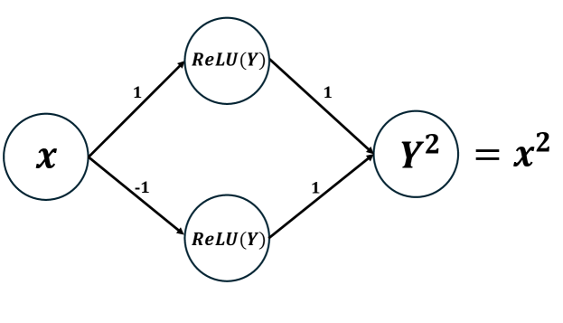
Figure 3: Subnetwork equivalent to operation of taking a square.

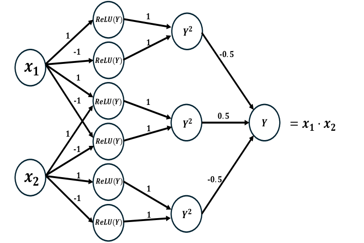
Figure 4: Subnetwork equivalent to the product operation.

B.2 Product of two values

To find a product of two values $x_{1}$ and $x_{2}$ one can use the formula $x_{1}\cdot x_{2}=0.5\cdot((x_{1}+x_{2})^{2}-x_{1}^{2}-x_{2}^{2})$. This leads us to the feedforward network structure in Figure 4.

B.3 Maximum of two values

The maximum operation can be expressed via a subnetwork with ReLU activation functions only, as follows. Observing that $\max\{x_{1},x_{2}\}=0.5\cdot(x_{1}+x_{2}+|x_{1}-x_{2}|)$ results in the corresponding network structure in Figure 5.

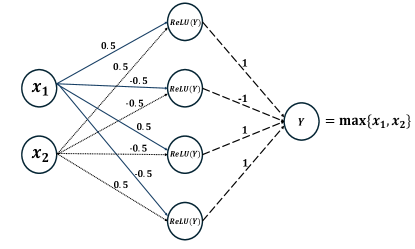
Figure 5: Subnetwork equivalent to a maximum of two values.

B.4 Softmax

The function $\mathrm{softmax}$ transforms a vector of real numbers to a probability distribution. That is, if ${\mathbf{x}}=(x_{1},\ldots,x_{n})\in^{n}$, then there is a multivariate function $SfMax:^{n}\xrightarrow[]{}^{n}$, so that

$$SfMax_{i}=\mathrm{softmax}(x_{i})=\frac{e^{x_{i}}}{\sum\limits_{j=i}^{n}e^{x_{j}}}$$

Then, $log(SfMax_{i})=x_{i}-\log\sum\limits_{j=i}^{n}e^{x_{j}}$, which is a composition of monotonic functions. This leads to the feedforward network structure in Figure 6.

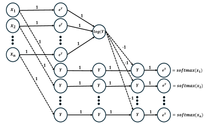
Figure 6: Subnetwork equivalent to one softmax node.

Appendix C Description of Iris Experiments

We trained a fully connected $\left[3\times 12\right]$ ReLU NN with a final $\left[1\times 3\right]$ linear layer, as well as a fully connected $\left[3\times 12\right]$ $\tanh$ NN with the same final $\left[1\times 3\right]$ linear layer, on the Iris dataset. The networks classify objects into three classes: Setosa, Versicolor, and Virginica, using two input features: Sepal Length and Sepal Width. The allocation of the data for these two variables in the three classes is shown in Figure 10. The input data were rescaled to be within the interval $\left[0,1\right]$.

Experiment 1: ReLU-Based Network with Random Inputs.

The ReLU network was pre-trained. We next introduced randomness to the input variables by modeling them as Beta-distributed with parameters $(2,2)$ and $(3,2)$, respectively. The pdfs of these input distributions are shown in Figure 10. The first is symmetric about 0.5 and the second is left-skewed.

In our first experiment, Example 3.10, we computed the exact cdf of the first output neuron (out of three) in the ReLU network before applying the softmax function. Due to the presence of a final linear layer, the output may contain negative values. To validate our computation, we compared it against a conditional ground truth obtained via extensive Monte Carlo simulations, where the empirical cdf was estimated using $10^{5}$ samples. As shown in Figure 1, both cdf plots coincide. The cdf values were computed at 100 grid points across the estimated support of the output, determined via the IBP procedure.

For further comparison, Figure 10 presents an approximation of the output pdf based on the previously computed cdf values. This is compared to a histogram constructed from Monte Carlo samples. Additionally, we include a Gaussian kernel density estimation (KDE) plot obtained from the sampled data using a smoothing parameter of $h=0.005$. The results indicate that our pdf approximation better represents the underlying distribution compared to KDE and tracks the histogram more closely.

Experiment 2: Bounding a Tanh-Based Network with ReLU Approximations.

In our second experiment, we used a pre-trained NN with a similar structure but replaced the ReLU activation functions in the first three layers with tanh. To approximate this network, we constructed two bounding fully connected NNs—one upper and one lower—using only ReLU activations.

We conducted computations in two regimes: one using 5 segments and another using 10 segments, into which both convex and concave regions of the tanh activation function at each neuron in the first three layers were divided. Over each segment, we performed piecewise linear approximations according to the procedure described in Section 3.2 and combined these approximations into three-layer ReLU networks with an additional final linear layer for both upper and lower bounds. The results of these approximations are shown in Figure 2. In the 10-segment regime, both the upper and lower approximations closely align with the original NN’s output.

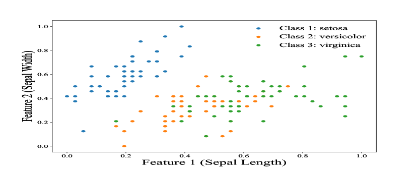
Figure 7: Plot of Sepal Width vs Sepal Length with class indication.

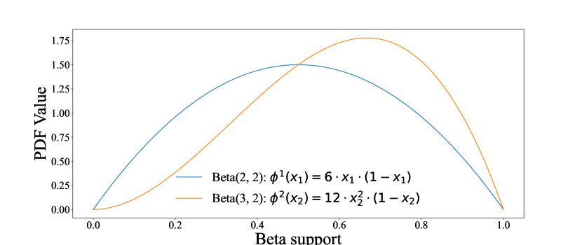
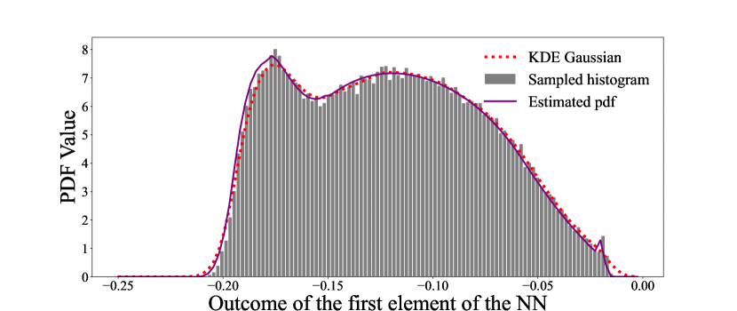
Figure 8: Plots of the $Beta(2,2)$ and $Beta(3,2)$ pdfs, resp.

Figure 9: Estimated output pdf compared with KDE with smoothing parameter $h=0.005$ and histogram of MC simulations.

Figure 10: Iris Dataset

References

- Abdelaziz et al. (2015) Abdelaziz, A., Watanabe, S., Hershey, J., Vincent, E., and Kolossa, D. Uncertainty propagation through deep neural networks. Proceedings of the Annual Conference of the International Speech Communication Association, INTERSPEECH, 2015-January:3561–3565, 2015. ISSN 2308-457X. Publisher Copyright: Copyright © 2015 ISCA.; 16th Annual Conference of the International Speech Communication Association, INTERSPEECH 2015 ; Conference date: 06-09-2015 Through 10-09-2015.
- Aeberhard & Forina (1992) Aeberhard, S. and Forina, M. Wine. UCI Machine Learning Repository, 1992. DOI: https://doi.org/10.24432/C5PC7J.
- Berzins (2023) Berzins, A. Polyhedral complex extraction from ReLU networks using edge subdivision. In Krause, A., Brunskill, E., Cho, K., Engelhardt, B., Sabato, S., and Scarlett, J. (eds.), Proceedings of the 40th International Conference on Machine Learning, volume 202 of Proceedings of Machine Learning Research, pp. 2234–2244. PMLR, 23–29 Jul 2023. URL https://proceedings.mlr.press/v202/berzins23a.html.
- Bibi et al. (2018) Bibi, A., Alfadly, M., and Ghanem, B. Analytic expressions for probabilistic moments of pl-dnn with gaussian input. In 2018 IEEE/CVF Conference on Computer Vision and Pattern Recognition, pp. 9099–9107, 2018. doi: 10.1109/CVPR.2018.00948.
- Bunel et al. (2019) Bunel, R., Lu, J., Turkaslan, I., Torr, P. H. S., Kohli, P., and Kumar, M. P. Branch and bound for piecewise linear neural network verification. ArXiv, abs/1909.06588, 2019. URL https://api.semanticscholar.org/CorpusID:202577669.
- Cybenko (1989) Cybenko, G. Approximation by superpositions of a sigmoidal function. Mathematics of Control, Signals and Systems, 2(4):303–314, 1989. doi: 10.1007/BF02551274. URL https://doi.org/10.1007/BF02551274.
- Efron et al. (2004) Efron, B., Hastie, T., Johnstone, I., and Tibshirani, R. Least angle regression. The Annals of Statistics, pp. 407–451, 2004. URL https://www.jstor.org/stable/3448465.
- Fawzi et al. (2018) Fawzi, A., Fawzi, H., and Fawzi, O. Adversarial vulnerability for any classifier. In Proceedings of the 32nd International Conference on Neural Information Processing Systems, NIPS’18, pp. 1186–1195, Red Hook, NY, USA, 2018. Curran Associates Inc.
- Ferrari et al. (2022) Ferrari, C., Mueller, M. N., Jovanović, N., and Vechev, M. Complete verification via multi-neuron relaxation guided branch-and-bound. In International Conference on Learning Representations, 2022. URL https://openreview.net/forum?id=l_amHf1oaK.
- Fisher (1936) Fisher, R. A. The use of multiple measurements in taxonomic problems. Annals of Human Genetics, 7:179–188, 1936. URL https://onlinelibrary.wiley.com/doi/10.1111/j.1469-1809.1936.tb02137.x.
- Gawlikowski et al. (2023) Gawlikowski, J., Tassi, C. R. N., Ali, M., Lee, J., Humt, M., Feng, J., Kruspe, A., Triebel, R., Jung, P., Roscher, R., Shahzad, M., Yang, W., Bamler, R., and Zhu, X. X. A survey of uncertainty in deep neural networks. Artificial Intelligence Review, 56:1513–1589, 2023. URL https://doi.org/10.1007/s10462-023-10562-9.
- Gehr et al. (2018) Gehr, T., Mirman, M., Drachsler-Cohen, D., Tsankov, P., Chaudhuri, S., and Vechev, M. Ai2: Safety and robustness certification of neural networks with abstract interpretation. In 2018 IEEE Symposium on Security and Privacy (SP), pp. 3–18, 2018. doi: 10.1109/SP.2018.00058.
- Goodfellow et al. (2014a) Goodfellow, I., Pouget-Abadie, J., Mirza, M., Xu, B., Warde-Farley, D., Ozair, S., Courville, A., and Bengio, Y. Generative adversarial nets. Advances in neural information processing systems, 27, 2014a.
- Goodfellow et al. (2014b) Goodfellow, I. J., Shlens, J., and Szegedy, C. Explaining and harnessing adversarial examples. CoRR, abs/1412.6572, 2014b. URL https://api.semanticscholar.org/CorpusID:6706414.
- Gowal et al. (2018) Gowal, S., Dvijotham, K., Stanforth, R., Bunel, R., Qin, C., Uesato, J., Arandjelović, R., Mann, T. A., and Kohli, P. On the effectiveness of interval bound propagation for training verifiably robust models. ArXiv, abs/1810.12715, 2018. URL https://api.semanticscholar.org/CorpusID:53112003.
- Hafiz & Bhat (2020) Hafiz, A. M. and Bhat, G. M. A survey of deep learning techniques for medical diagnosis. In Tuba, M., Akashe, S., and Joshi, A. (eds.), Information and Communication Technology for Sustainable Development, pp. 161–170, Singapore, 2020. Springer Singapore. ISBN 978-981-13-7166-0.
- Hoeffding (1963) Hoeffding, W. Probability inequalities for sums of bounded random variables. Journal of the American Statistical Association, 58(301):13–30, 1963. ISSN 01621459, 1537274X. URL http://www.jstor.org/stable/2282952.
- Hornik et al. (1989) Hornik, K., Stinchcombe, M., and White, H. Multilayer feedforward networks are universal approximators. Neural Networks, 2(5):359–366, 1989. ISSN 0893-6080. doi: https://doi.org/10.1016/0893-6080(89)90020-8. URL https://www.sciencedirect.com/science/article/pii/0893608089900208.
- Hosseini et al. (2017) Hosseini, H., Xiao, B., and Poovendran, R. Google’s cloud vision api is not robust to noise. In 2017 16th IEEE International Conference on Machine Learning and Applications (ICMLA), pp. 101–105, 2017. doi: 10.1109/ICMLA.2017.0-172.
- Hüllermeier & Waegeman (2021) Hüllermeier, E. and Waegeman, W. Aleatoric and epistemic uncertainty in machine learning: an introduction to concepts and methods. Machine Learning, 110(3):457–506, 2021. doi: 10.1007/s10994-021-05946-3. URL https://doi.org/10.1007/s10994-021-05946-3.
- Ji et al. (2020) Ji, W., Ren, Z., and Law, C. K. Uncertainty propagation in deep neural network using active subspace, 2020. URL https://arxiv.org/abs/1903.03989.
- Katz et al. (2017) Katz, G., Barrett, C., Dill, D. L., Julian, K., and Kochenderfer, M. J. Reluplex: An efficient smt solver for verifying deep neural networks. In Majumdar, R. and Kunčak, V. (eds.), Computer Aided Verification, pp. 97–117, Cham, 2017. Springer International Publishing. ISBN 978-3-319-63387-9.
- Katz et al. (2019) Katz, G., Huang, D. A., Ibeling, D., Julian, K., Lazarus, C., Lim, R., Shah, P., Thakoor, S., Wu, H., Zeljić, A., Dill, D. L., Kochenderfer, M. J., and Barrett, C. The marabou framework for verification and analysis of deep neural networks. In Dillig, I. and Tasiran, S. (eds.), Computer Aided Verification, pp. 443–452, Cham, 2019. Springer International Publishing. ISBN 978-3-030-25540-4.
- Krapf et al. (2024) Krapf, T., Hagn, M., Miethaner, P., Schiller, A., Luttner, L., and Heinrich, B. Piecewise linear transformation – propagating aleatoric uncertainty in neural networks. Proceedings of the AAAI Conference on Artificial Intelligence, 38(18):20456–20464, Mar. 2024. doi: 10.1609/aaai.v38i18.30029. URL https://ojs.aaai.org/index.php/AAAI/article/view/30029.
- Lasserre (2021) Lasserre, J. B. Simple formula for integration of polynomials on a simplex. BIT, 61(2):523–533, jun 2021. ISSN 0006-3835. doi: 10.1007/s10543-020-00828-x. URL https://doi.org/10.1007/s10543-020-00828-x.
- Raghu et al. (2017) Raghu, M., Poole, B., Kleinberg, J., Ganguli, S., and Sohl-Dickstein, J. On the expressive power of deep neural networks. In Precup, D. and Teh, Y. W. (eds.), Proceedings of the 34th International Conference on Machine Learning, volume 70 of Proceedings of Machine Learning Research, pp. 2847–2854. PMLR, 06–11 Aug 2017. URL https://proceedings.mlr.press/v70/raghu17a.html.
- Rao (1962) Rao, R. R. Relations between Weak and Uniform Convergence of Measures with Applications. The Annals of Mathematical Statistics, 33(2):659 – 680, 1962. doi: 10.1214/aoms/1177704588. URL https://doi.org/10.1214/aoms/1177704588.
- Shi et al. (2024) Shi, Z., Jin, Q., Kolter, Z., Jana, S., Hsieh, C.-J., and Zhang, H. Neural network verification with branch-and-bound for general nonlinearities. ArXiv, abs/2405.21063, 2024. URL https://arxiv.org/pdf/2405.21063.
- Sicking et al. (2022) Sicking, J., Akila, M., Schneider, J. D., Huger, F., Schlicht, P., Wirtz, T., and Wrobel, S. Tailored uncertainty estimation for deep learning systems. ArXiv, abs/2204.13963, 2022. URL https://api.semanticscholar.org/CorpusID:248475977.
- Sudjianto et al. (2020) Sudjianto, A., Knauth, W., Singh, R., Yang, Z., and Zhang, A. Unwrapping the black box of deep relu networks: Interpretability, diagnostics, and simplification. ArXiv, abs/2011.04041, 2020. URL https://api.semanticscholar.org/CorpusID:226281525.
- van Buuren & Groothuis-Oudshoorn (2011) van Buuren, S. and Groothuis-Oudshoorn, K. mice: Multivariate imputation by chained equations in r. Journal of Statistical Software, 45(3):1–67, 2011. doi: 10.18637/jss.v045.i03. URL https://www.jstatsoft.org/index.php/jss/article/view/v045i03.
- Wang et al. (2022) Wang, Z., Albarghouthi, A., Prakriya, G., and Jha, S. Interval universal approximation for neural networks. Proc. ACM Program. Lang., 6(POPL), jan 2022. doi: 10.1145/3498675. URL https://doi.org/10.1145/3498675.
- Weng et al. (2019) Weng, L., Chen, P.-Y., Nguyen, L., Squillante, M., Boopathy, A., Oseledets, I., and Daniel, L. PROVEN: Verifying robustness of neural networks with a probabilistic approach. In Chaudhuri, K. and Salakhutdinov, R. (eds.), Proceedings of the 36th International Conference on Machine Learning, volume 97 of Proceedings of Machine Learning Research, pp. 6727–6736. PMLR, 09–15 Jun 2019. URL https://proceedings.mlr.press/v97/weng19a.html.
- Wu et al. (2024a) Wu, H., Isac, O., Zeljić, A., Tagomori, T., Daggitt, M., Kokke, W., Refaeli, I., Amir, G., Julian, K., Bassan, S., Huang, P., Lahav, O., Wu, M., Zhang, M., Komendantskaya, E., Katz, G., and Barrett, C. Marabou 2.0: A versatile formal analyzer of neural networks. In Gurfinkel, A. and Ganesh, V. (eds.), Computer Aided Verification, pp. 249–264, Cham, 2024a. Springer Nature Switzerland. ISBN 978-3-031-65630-9.
- Wu et al. (2024b) Wu, H., Isac, O., Zeljic, A., Tagomori, T., Daggitt, M. L., Kokke, W., Refaeli, I., Amir, G., Julian, K., Bassan, S., Huang, P., Lahav, O., Wu, M., Zhang, M., Komendantskaya, E., Katz, G., and Barrett, C. W. Marabou 2.0: A versatile formal analyzer of neural networks. In Gurfinkel, A. and Ganesh, V. (eds.), Computer Aided Verification - 36th International Conference, CAV 2024, Montreal, QC, Canada, July 24-27, 2024, Proceedings, Part II, volume 14682 of Lecture Notes in Computer Science, pp. 249–264. Springer, 2024b. doi: 10.1007/978-3-031-65630-9“˙13. URL https://doi.org/10.1007/978-3-031-65630-9_13.
- Xu et al. (2020) Xu, K., Shi, Z., Zhang, H., Huang, M., Chang, K.-W., Kailkhura, B., Lin, X., and Hsieh, C.-J. Automatic perturbation analysis on general computational graphs. ArXiv, abs/2002.12920, 2020. URL https://api.semanticscholar.org/CorpusID:211572699.
- Yurtsever et al. (2020) Yurtsever, E., Lambert, J., Carballo, A., and Takeda, K. A survey of autonomous driving: Common practices and emerging technologies. IEEE Access, 8:58443–58469, 2020. doi: 10.1109/ACCESS.2020.2983149.
- Zhang & Shin (2021) Zhang, B. and Shin, Y. C. An adaptive gaussian mixture method for nonlinear uncertainty propagation in neural networks. Neurocomputing, 458:170–183, 2021. ISSN 0925-2312. doi: https://doi.org/10.1016/j.neucom.2021.06.007. URL https://www.sciencedirect.com/science/article/pii/S0925231221009024.
- Zhang et al. (2018) Zhang, H., Weng, T.-W., Chen, P.-Y., Hsieh, C.-J., and Daniel, L. Efficient neural network robustness certification with general activation functions. In Proceedings of the 32nd International Conference on Neural Information Processing Systems, NIPS’18, pp. 4944–4953, Red Hook, NY, USA, 2018. Curran Associates Inc. URL https://dl.acm.org/doi/abs/10.5555/3327345.3327402.
- Zhang et al. (2020) Zhang, H., Chen, H., Xiao, C., Gowal, S., Stanforth, R., Li, B., Boning, D., and Hsieh, C.-J. Towards stable and efficient training of verifiably robust neural networks. In International Conference on Learning Representations, 2020. URL https://openreview.net/forum?id=Skxuk1rFwB.
- Ziegler (1995) Ziegler, G. M. Lectures on polytopes. Springer-Verlag, New York, 1995.