Box Confidence Depth: simulation-based inference with hyper-rectangles

Abstract

This work presents a novel simulation-based approach for constructing confidence regions in parametric models, which is particularly suited for generative models and situations where limited data and conventional asymptotic approximations fail to provide accurate results. The method leverages the concept of data depth and depends on creating random hyper-rectangles, i.e. boxes, in the sample space generated through simulations from the model, varying the input parameters. A probabilistic acceptance rule allows to retrieve a Depth-Confidence Distribution for the model parameters from which point estimators as well as calibrated confidence sets can be read-off. The method is designed to address cases where both the parameters and test statistics are multivariate.

,

1 Introduction

In many scientific domains, researchers face the challenge of evaluating complex statistical models in which the likelihood function is either computationally intractable or prohibitively expensive to calculate. This has led to the development and increasing popularity of likelihood-free inference methods, which offer powerful alternatives for parameter estimation and model comparison. These methodologies leverage simulations, enabling inference through the comparison of observed data with simulated outcomes generated from the model under various parameter settings. In Bayesian inference, these include Approximate Bayesian Computation (Rubin, 1984; Pritchard et al., 1999; Sisson et al., 2018), Bayesian Synthetic Likelihood (Wood, 2010; Price et al., 2018), Neural Likelihood and Posterior Estimation (Rezende and Mohamed, 2015; Papamakarios, Sterratt and Murray, 2019). In the frequentist setting, after the foundational work of Gourieroux, Monfort and Renault (1993), only recent years have seen advancements in likelihood-free inference (Masserano et al., 2022; Xie and Wang, 2022; Dalmasso et al., 2024).

This study focuses on frequentist inference, targeting the construction of calibrated confidence intervals and regions across simulation-based models and non-standard regularity conditions. The proposed approach provides a unified strategy for inference that seamlessly accommodates both univariate and multivariate parameters. This is achieved by means of a depth function (Liu, 1990), that allows defining nested confidence sets across all confidence levels, offering researchers a comprehensive visualization of parametric uncertainty. A significant aspect of the proposed methodology is its ability to operate without requiring data to be necessarily reduced to a scalar summary statistic. Raw data can be utilized directly, enhancing the flexibility and automation of the inference process, and inference from diverse test statistics, linked to model-specific information, can be combined in a natural manner. As a byproduct of the procedure, the method also yields consistent point estimators for model parameters.

The rest of the paper is organized as follows. Section 2 reviews recent developments in simulation-based inference. Section 3 outlines the sampling methodology used to build the Confidence Depth, discusses its theoretical underpinnings, and addresses some computational aspects. Section 4 discusses various examples from either classical models such as Generalized Linear Models (GLMs), as well as models from the field of Likelihood Free Inference (LFI) and reports simulation studies. A discussion is provided in Section 5.

2 Simulation based inference

Consider a parametric model $p(y|\theta)$, with $\theta$ a finite-dimensional parameter. We denote with $y^{\text{obs}}$ the observed data, of size $n$, with ${t}:\mathbb{R}^{n}\rightarrow\mathbb{R}^{d}$ a collection of summary statistics of $d\leq n$ components, with ${t^{\text{obs}}}=t(y^{\text{obs}})$ the observed summary statistics.

The key idea of Simulation Based Inference (SBI) is that inference can rely on simulations from the same process responsible for producing observed data. Once pseudo-observations are generated from the model across various parameters values, the plausibility of the parameter used in the simulation can be assessed, based on comparison with the original data $y^{\text{obs}}$.

The most popular method for SBI in Bayesian inference is Approximate Bayesian Computation (ABC), introduced by Rubin (1984) and further developed by Pritchard et al. (1999). ABC aims to generate datasets that mimic the observed sample using as proposals for $\theta$ draws from the prior distribution. Parameter values that generate synthetic observations closely matching the real observation, up to a certain tolerance $\varepsilon$, i.e. $d(y,y^{\text{obs}})<\varepsilon$, are retained. The distance $d(\cdot,\cdot)$ between pseudo and actual data is generally assessed on a set of summary statistics that are informative for the model. Intuitively, if the synthetic data match the observed data, the model parameters used in the simulations are plausible for the model under consideration and in turns, they are associated to higher likelihood function. Several enhancements to the basic ABC algorithm have been proposed over time, see Marjoram et al. (2003); Marin et al. (2012); Del Moral and Murray (2015); Frazier et al. (2018); Bernton et al. (2019); Rotiroti and Walker (2024) and references therein. The approximation in ABC is considered non parametric, as the shape of the likelihood and the posterior is not specified but obtained by rejection Monte Carlo. Parametric approximations of likelihood functions (and posteriors) in simulation-based settings have seen significant advancements in recent years, largely due to the growing influence of Machine Learning and Deep Learning techniques. Two prominent approaches are Bayesian Synthetic likelihood (Wood, 2010; Price et al., 2018; Frazier et al., 2023), which employs conditional density estimators based on a multivariate Gaussian model and the family of Neural Posterior Estimation methods (Rezende and Mohamed, 2015; Papamakarios, Sterratt and Murray, 2019) employing more flexible conditional density estimators, as normalizing flows which better suited for high-dimensional data and complex models. Machine Learning methods have been heavily employed in Neural Ratio Estimation (NRE) (Hermans, Begy and Louppe, 2020; Thomas et al., 2022) that estimates the ratio between the likelihood $p(y|\theta)$ and data marginal $p(y)$, that is $r(y,\theta)=p(y|\theta)/p(y)$, by training a classifier to distinguish datasets generated from the conditional and the marginal model.

In the frequentist paradigm, ratio estimation was adopted by Dalmasso et al. (2024) to approximate the likelihood ratio statistic. In particular, once the quantity $r(y,\theta)$ is approximated by means of the classifier trained on the conditional model and on models simulated using a reference distribution for the parameter of interest, the empirical quantiles of level $\alpha$ are used to build confidence sets. Recently, Kuchibhotla, Balakrishnan and Wasserman (2024) developed a methodology for constructing confidence intervals and sets with bounded coverage errors by utilizing data subsampling. Nevertheless, the strategy is not purely likelihood-free, as it relies on Maximum Likelihood estimation, similarly to the Bootstrap approach (Efron, 1979, 2003).

3 Box-Confidence Depth

Assume that it is possible to generate data from the parametric model $p(y|\theta)$, with $\theta\in\Theta\subseteq\mathbb{R}^{p}$. Let ${\theta_{0}}$ be the true value of $\theta$. We assume that the model is correctly specified, so that ${p(y|\theta_{0})}$ corresponds to the true data generating process. Let $\pi(\theta)$ be a proposal distribution for the unknown parameter. Here, the proposal distribution is assumed to be uniform in a subset of the parameter space $\Theta^{b}\subset\Theta$. This boundedness of $\Theta^{b}$ is technically necessary to ensure computational feasibility, and guidelines to choose $\Theta^{b}$ are discussed below.

The proposed method consists in drawing $\theta^{*}$ from $\pi(\theta)$ and, for each $\theta^{*}$, generate two pseudo-samples from the model ${p(y|\theta^{*})}$, denoted as $y^{*1}$ and $y^{*2}$. Summary statistics $t^{*1}$ and $t^{*2}$ are then computed from $y^{*1}$ and $y^{*2}$, respectively, each of dimension $d$. The proposal $\theta^{*}$ is accepted if the observed summary statistic $t^{\text{obs}}$, computed from the actual observed data $y^{\text{obs}}$, falls within a region defined by $t^{*1}$ and $t^{*2}$. This region can be conceptualized as a $d-$dimensional hyper-rectangle, called Box and denoted as $\mathcal{B}_{t}^{*}$, in the space of summary statistics, with $t^{*1}=(t_{1}^{*1},\ldots,t_{d}^{*1})$ and $t^{*2}=(t_{1}^{*2},\ldots,t_{d}^{*2})$ defining its edges, i.e.

$$\mathcal{B}_{t}^{*}=\times_{j=1}^{d}[t_{j}^{*(1)},t_{j}^{*(2)}],$$

where $t_{j}^{*(1)}$ and $t_{j}^{*(2)}$ are the order statistics along the $j$-th coordinate ($j=1,\ldots,d)$. Equivalently, the parameter $\theta^{*}$ is accepted if $t_{1}^{*(1)}<t_{1}^{\text{obs}}<t_{1}^{*(2)},\>t_{2}^{*(1)}<t_{2}^{\text{obs}}<t_{2}^{*(2)},\>\ldots,\>t_{d}^{*(1)}<t_{d}^{\text{obs}}<t_{d}^{*(2)}.$ Figure 1 illustrates this concept in dimension $d=2$ and the algorithm is outlined in Algorithm 1.

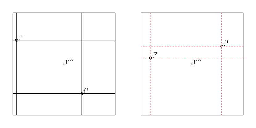
Figure 1: Two examples of summary statistics, $t^{*1}=(t^{*1}_{1},t^{*1}_{2})$ and $t^{*2}=(t^{*2}_{1},t^{*2}_{2})$ computed on simulated pseudo-samples. Left: the proposal parameter would be accepted as the observed $t^{\text{obs}}$ lies within the Box. Right: the proposal is rejected as $t^{\text{obs}}$ falls outside this Box.

The procedure described seeks to learn a data-dependent distribution over the parameter space non-parametrically, utilizing a rejection algorithm, as in ABC, instead of assuming a closed-form model for summary statistics. It differs from ABC because it focuses on establishing an ordering in the sample space to determine confidence level measure over the parameter space, which is consistent with the frequentist view on confidence and uncertainty. In particular, the acceptance rule does not make use of a distance function and a threshold parameter, but it is based on a series of inequalities. Note that, since establishing a meaningful ordering in the sample space becomes challenging in presence of multivariate data and summary statistics, the procedure in practice utilizes a measure of centrality of observed data with respect to simulated data, which corresponds to an ordering from the center outwards.

Proposals $\theta^{*}$ associated with a high centrality of the observed sample lead to frequent acceptance. This results in an empirical Monte Carlo-based measure of confidence and an ordering within the parameter space. The accepted $\theta^{*}$ are distributed as

$$\mathcal{CD}^{\text{box}}(\theta):\Theta\mapsto R^{+},$$

called Box-Confidence Depth, which assigns a measure of centrality or ”depth” to each parameter, with higher values indicating that the parameter is more central or representative of the observed data.

3.1 Scalar-scalar case

To formalize the properties of the function $\mathcal{CD}^{\text{box}}(\theta)$ in relation to confidence intervals and frequentist tests, it is useful to initially consider the scenario where $\theta\in\mathrm{R}$ and $d=1$. In this case, the Box reduces to an interval with endpoints $t(y^{*}_{1})$ and $t(y^{*}_{2})$ and the proposed $\theta^{*}$ is accepted if and only if $t(y^{\text{obs}})\in[t^{*(1)},t^{*(2)}]$.

Assumption 1.

The statistic $t:\mathcal{Y}\mapsto\mathcal{T}\in\mathrm{R}$ is one-dimensional and $0<Var(t(y)|\theta)<\infty$ for $\pi$-almost all $\theta$.

The assumption that $Var(t(y)|\theta)>0$ for $\pi$-almost all $\theta$ ensures that the intervals of the form $[t^{(1)},t^{(2)}]$ have positive probability of being non-empty.

Assumption 2.

The support $\Theta^{b}$ is chosen such that

$$\sup_{\theta\in\Theta^{b}}F_{t}(t^{\text{obs}}|\theta)>1-k\text{ and }\inf_{\theta\in\Theta^{b}}F_{t}(t^{\text{obs}}|\theta)<k,$$

where the function $F_{t}(t^{\text{obs}}|\theta)$ is the cumulative density function of $t(y)$, computed on the value of the observed summary statistic $t^{\text{obs}}$ and with $k$ of the same order of the machine tolerance.

Lemma 3.1.

For a scalar parameter $\theta$, under Assumption 1 the Box-Confidence Depth is

$$\mathcal{CD}^{\text{box}}(\theta)\propto F_{t}(t^{\text{obs}}|\theta)[1-F_{t}(t^{\text{obs}}|\theta)].$$

Proof.

Let $\theta\in\Theta$, and consider a pair of statistics following the pushed-forward distribution induced by the summary statistic $t$ applied to $y\sim p(y|\theta)$, i.e. $(t^{*1},\;t^{*2})\overset{iid}{\sim}t_{\#}p(y|\theta)$. One can compute the probability of acceptance of $\theta$ as follows:

$$\Pr(t^{(1)}\leq t^{\text{obs}}<t^{(2)}|\theta)=\Pr(t^{*1}\leq t^{\text{obs}}<t^{*2}|\theta)+\Pr(t^{*1}>t^{\text{obs}}\geq t^{*2}|\theta)$$

$$=\Pr(t^{*1}\leq t^{\text{obs}},t^{\text{obs}}<t^{*2}|\theta)+\Pr(t^{*1}>t^{\text{obs}},t^{\text{obs}}\geq t^{*2}|\theta)$$

$$=F_{t}(t^{\text{obs}}|\theta)[1-F_{t}(t^{\text{obs}}|\theta)]+F_{t}(t^{\text{obs}}|\theta)[1-F_{t}(t^{\text{obs}}|\theta)]$$

$$=2F_{t}(t^{\text{obs}}|\theta)[1-F_{t}(t^{\text{obs}}|\theta)]$$

$$\propto F_{t}(t^{\text{obs}}|\theta)[1-F_{t}(t^{\text{obs}}|\theta)].$$

Under Assumption 2 we obtain the target distribution by a usual rejection sampling argument. ∎

Lemma 3.2.

Under Assumption 1:
i) $F_{t}(t^{\text{obs}}|\theta)$ as a function of $\theta$ is a one-sided $p$-value function,
ii)  $F_{t}(t^{\text{obs}}|\theta)$ is a Confidence Distribution (CD) when $F_{t}(t^{\text{obs}}|\theta)$ is stochastically increasing in $\theta$.

Proof.

Statement $i)$ follows immediately from the definition of $F_{t}$ in Lemma 3.1. For $ii)$, in general, a function $H(y,\theta)$ on $\mathcal{Y}\times\Theta\rightarrow[0,1]$ is a CD for $\theta$ if (see e.g. Xie and Singh, 2013): a) for each given $y\in\mathcal{Y},H(\cdot)$ is a cumulative distribution function on $\Theta$; b) at $\theta=\theta_{0}$, $H(y^{\text{obs}},\theta_{0})$, as a function of the sample $y^{\text{obs}}$, follows a $\text{Uniform}[0,1]$ distribution. By construction $F_{t}(t^{\text{obs}}|\theta_{0})\in[0,1]$, furthermore, if $t$ is stochastically increasing in $\theta$, then $F_{t}(t^{\text{obs}}|\theta^{\prime})<F_{t}(t^{\text{obs}}|\theta^{\prime\prime})$ for $\theta^{\prime\prime}>\theta^{\prime}.$ By properties of the $p$-value function and for $u\in[0,1]$ $Pr(F_{t}(t^{\text{obs}}|\theta)<u)=Pr(t^{\text{obs}}<F_{t}^{-1}(u|\theta))$ is constant when $t^{\text{obs}}$ is drawn from $F_{t}(\cdot|\theta)$. ∎

Lemma 3.3.

Let $\hat{\theta}$ be the maximizer of $\mathcal{CD}^{\text{box}}(\theta)$. Then, under Assumption 1 $\hat{\theta}$ is median unbiased, i.e.

$$Pr_{\theta_{0}}(\hat{\theta}\leq\theta_{0})=1/2.$$ (1)

Proof.

By definition $\hat{\theta}=\underset{\theta}{\arg\max}\>F_{t}(t^{\text{obs}}|\theta)[1-F_{t}(t^{\text{obs}}|\theta)].$ Since $F_{t}(t^{\text{obs}}|\theta)\in[0,1]$, the expression is maximum when the function $x(1-x)$ is maximum with $x$ in $[0,1]$, which is $F_{t}(t^{\text{obs}}|\hat{\theta})=0.5$. Then, applying $F_{t}$ to both sides of the inequality of Equation (1) it follows that $Pr_{\theta_{0}}(F_{t}(t^{\text{obs}}|\hat{\theta})<F_{t}(t^{\text{obs}}|\theta_{0}))=$ $Pr_{\theta_{0}}(0.5<F_{t}(t^{\text{obs}}|\theta_{0}))=1/2.$ ∎

Median unbiasedness is a desired property as it guarantees consistency of the estimator (Schweder and Hjort, 2016). Additionally, this property is preserved also for any one-to-one reparametrizations (Kenne Pagui, Salvan and Sartori, 2017; Kuchibhotla, Balakrishnan and Wasserman, 2024).

Remark 1.

Note that differently from a Confidence Distribution, the shape of $\mathcal{CD}^{\text{box}}(\theta)$ does not assume that $t$ is stochastically ordered in $\theta$. In particular, if $F_{t}(t^{\text{obs}}|\theta)$ is not monotone in $\theta$, the function $\mathcal{CD}^{\text{box}}(\theta)$ can be multimodal. Figure 2 illustrates this possibility.

Remark 2.

Note that if the proposal $\pi(\theta)$ is centered on the confidence median, and the function $\mathcal{CD}^{\text{box}}(\theta)$ is symmetric, then the expected acceptance probability is 1/4. Note that if the proposal $\pi(\theta)$ is centered on the confidence median, and the function $\mathcal{CD}^{\text{box}}(\theta)$ is symmetric, then the expected acceptance probability is 1/4. This can be regarded as a practical guideline to tune the proposal.

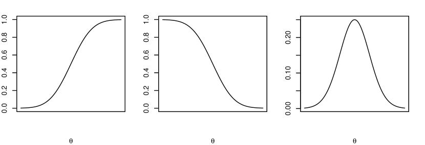
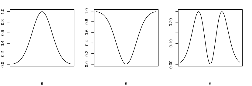
Figure 2: Top panels: an instance of a monotone $p$-value function $F_{t}(t^{\text{obs}}|\theta)$ (left), $1-F_{t}(t^{\text{obs}}|\theta)$ (center), and their product (right). Bottom panels: a non a monotone $p$-value function where the resulting Confidence-Depth is multimodal.

Input: Proposal distribution $\pi(\theta)$, number of iterations $R$, summary statistic function $t(\cdot)$, observed statistic $t^{\text{obs}}=t(y^{\text{obs}})$

Output: Accepted samples $\theta^{*}$

for $j\leftarrow 1$ to $R$ do

    Sample $\theta^{*}_{j}\sim\pi(\theta)$;

    Sample $y_{j}^{*1},y_{j}^{*2}\sim f(y;\theta_{j}^{*})$;

    Compute $t_{j}^{*1}=t(y_{j}^{*1})$,  $t_{j}^{*2}=t(y_{j}^{*2})$;

    if $t^{\text{obs}}\in\mathcal{B}(t_{j}^{*1},t_{j}^{*2})$ then

       Accept $\theta_{j}^{*}$;

      

    end if

   

end for

return Accepted samples $\theta^{*}$

Algorithm 1 Accept-Reject Box-CD

3.2 Relation to confidence intervals

Let us write $F_{t}(\theta)$ shortly for $F_{t}(t^{\text{obs}}|\theta)$. Define an equi-tailed confidence interval of size $1-\alpha$ as $C_{1-\alpha}=\{\theta|F_{t}(\theta)>\alpha/2\text{\;and\>}F_{t}(\theta)<(1-\alpha/2)\}$. Denote by $Q_{Z}(\cdot)$ the function s.t. for $p\in(0,1)$ and $Z,\zeta\in(0,1)$, $Q_{Z}(p)=\zeta$ if $\int 1_{Z<\zeta}dZ=p$.

Theorem 3.4.

For a scalar parameter $\theta$ and $\alpha\in(0,1)$ the following relation holds:

$$\mathcal{CD}^{\text{box}}(\theta)\geq Q_{\mathcal{CD}^{\text{box}}(\theta)}(\alpha)\Leftrightarrow\theta\in C_{1-\alpha}.$$

Proof.

Consider the piecewise linear function $g(F_{t})=-|F_{t}-0.5|\in[-0.5,0]$. From its definition, the set $C_{1-\alpha}$ can be written as $\{\theta|$ $g(F_{t})\geq-0.5+\alpha/2\}$. Since the image of $g$ is $[-0.5,0]$ and the function is linear in $F_{t}$, if ${g(F_{t})}\geq-0.5+\alpha/2$ then ${g(F_{t})}\geq Q_{g}(\alpha)$. Applying the monotone transformation $h(F_{t})=2g(F_{t})\text{sign}(F_{t}-0.5)+F_{t}=2(0.5-F_{t})+F_{t}=F_{t}(1-F_{t})$ which is order preserving, it directly follows that $Q_{\mathcal{CD}^{\text{box}}(\theta)}(\alpha)={g(F_{t})}$. This concludes the proof as $C_{1-\alpha}$ can be written as $\{\theta|$ $\mathcal{CD}^{\text{box}}(\theta)\geq Q_{\mathcal{CD}^{\text{box}}(\theta)}(\alpha)\}$. ∎

Theorem 3.4 outlines how to define confidence intervals via the Box-CD method. Indeed, the accepted values from Algorithm 1 are draws from $\theta^{*}\sim\text{Bernoulli}(\mathcal{CD}^{\text{box}}(\theta))$. Thus, it is sufficient to obtain a continuous approximation of the function $\mathcal{CD}^{\text{box}}(\theta)$. Specifically, any Machine Learning classification algorithm that outputs classification probabilities can be trained using proposals drawn from $\pi(\theta)$ as inputs, while the acceptance rule’s outcomes (0 or 1) as labels. Alternatively, the same task can be obtained by density estimation starting from the values $\theta^{*}$ accepted from Algorithm 1. From the parametric approximation (or density estimation) of the function $\mathcal{CD}^{\text{box}}(\theta)$, the quantiles can be obtained.

3.3 Mutivariate case: center-outward ordering

In classical statistics, when multiple statistics are collected ($d>1$), assessing the $p$-value of a precise null hypothesis involves computing the tail area probability of an event in dimension $d$. This process is complex and involves several considerations, particularly due to the dependence of the statistics used. In practice, the joint distribution is often only well-defined for Gaussian distributed test statistics, limiting the applicability to other distributions. It is generally preferred to reduce the information in a one dimensional statistic, even when the inference is on a parameter vector $(p>1)$, such as the Likelihood Ratio test (LR), since in contrast to univariate data, multivariate data lacks a natural method for ordering.

On the other side, to address the problem of ordering in multidimensional settings, researchers have developed various techniques leveraging Data Depth concepts. Data Depth (DD) functions provide a measure of centrality within multivariate sample spaces quantifying how deep a point is relative to a multivariate probability distribution or data cloud. This centrality measure allows for a center-outward ordering of points in any dimension to ultimately delineate nested central regions. For example, the Simplicial Depth (SD) method introduced by Liu (1990) determines the depth of a point by evaluating its presence within all combinations of simplex formed by the data points. When examining the univariate counterpart of the SD, i.e. two independent observations drawn from a univariate cumulative distribution function, the SD is reduced to the form $\text{SD}_{1}(x)=2F(x)[1-F(x)]$, and the point that maximises $\text{SD}_{1}(x)$ corresponds to the median of the population. Note that the definition resembles that of the Box-CD function $\mathcal{CD}^{\text{box}}(\theta)$ in the scalar case. Another well known DD function is the Tukey’s Depth (or Half-space Depth. HD). In one dimension it is used as the $p$-value for bilateral tests:

$$\text{HD}_{1}=2\min\{Pr(Y\leq y^{\text{obs}}\mid\theta),Pr(Y\geq y^{\text{obs}}\mid\theta)\}.$$

The HD function in the multivariate case requires the definition of a convex hull, which is the intersection of all halfspaces containing all sample points. The level sets of the HD are defined as the intersections of halfspaces containing $k<n$ sample points.

Liu, Liu and Xie (2022) consider the concept of DD to define Confidence Distributions for multivariate parameters, called depth CDs, by ranking parameter values instead of data points. They propose to use the distribution of non-parametric bootstrap estimates to recover an approximate depth CD, motivated by the fact that algorithms for reconstructing half-space and simplicial depths either rely on approximations in dimensions larger than 3 or computationally demanding procedures (Laketa and Nagy, 2023).

The Box-CD approach, which is based on ordering the sample space having a fixed reference $y^{\text{obs}}$, induces an ordering on the parameter space, similarly to the idea of the depth-CD of Liu, Liu and Xie (2022). The following lemma establishes a connection with the depth concept.

Lemma 3.5.

For two parameter points $\theta^{*}$ and $\theta^{**}$ within $\Theta$ and with their corresponding random Boxes $\mathcal{B}_{t}^{*}$, $\mathcal{B}_{t}^{**}$ , it holds that

$$Pr(t^{\text{obs}}\in\mathcal{B}_{t}^{*})<Pr(t^{\text{obs}}\in\mathcal{B}_{t}^{**})\Leftrightarrow\mathcal{CD}^{\text{box}}(\theta^{*})<\mathcal{CD}^{\text{box}}(\theta^{**}).$$

Note that Lemma 3.5 is not restricted to the case $p=1$. Indeed, $\theta$ can be a vector without compromising the definition. This means that the function $\mathcal{CD}^{\text{box}}(\theta)$ is higher when the random Box $\mathcal{B}_{t}^{*}$ contains the observed sample often, or equivalently, that the proposal $(\theta^{*},y^{*1},y^{*2})$ is well centered with respect to the generating process that provided $y^{\text{obs}}$. Beyond the application of the idea to simulation-based inference, as a Depth function $\mathcal{CD}^{\text{box}}(\theta)$ relies on hyper-rectangles to determine a centrality measure. This approach reduces the complexity associated with relying on simplexes as in the SD method.

3.4 Relation to Confidence sets and properties of the Box-CD function

Remark 1 plays a crucial role in generalizing the characteristics of the Box-CD function to the multivariate statistical context $(d>1)$. Since the test statistic $t$ does not need to be stochastically ordered either in one dimension, whether the components of $t$ are positively or negatively dependent does not influence the definition of the depth function.

We can generalize Lemma 3.4 to the general case of confidence sets assuming $\theta\in\mathrm{R}^{p}$. Define $M=\max_{\theta}\mathcal{CD}^{\text{box}}(\theta)$.

Theorem 3.6.

The region $C_{1-\alpha}=\{\theta|\mathcal{CD}^{\text{box}}(\theta)\geq\alpha M\}$ defines a confidence set with confidence level $1-\alpha$.

Proof.

The exact calibration property in the multivariate parameter case follows immediately by the definition. In fact,

$$Pr_{\theta_{0}}(\mathcal{CD}^{\text{box}}(\theta)>{Q_{\mathcal{CD}}}(\alpha))=\alpha,$$

indicating that when considering $\mathcal{CD}^{\text{box}}(\theta)$ as a global test statistic, akin to the log-likelihood ratio, $C_{1-\alpha}$ has the nominal coverage property. ∎

Remark 3.

Note that, even if the Algorithm 1 for deriving the Confidence depth function relies on the definition of hyper-rectangles (in the space of summary statistics), the confidence regions are curved regions (see Figure 5).

Lemma 3.7.

The Box-CD function is invariant under any transformation which is order preserving (up to the sign) applied individually to the components of $t$.

Proof.

Define the transformation $w(t):t\in\mathrm{R^{d}}\mapsto w\in\mathrm{R^{d}}$ as a bijective, component-wise function, where $w_{j}(t):t_{j}\mapsto w_{j}$ represents the monotonic transformation applied specifically to the $j$-th component of the statistic $t$. Then $w_{j}^{\prime}>w_{j}\Leftrightarrow\{t_{j}^{\prime}>t_{j}\text{ or }t_{j}^{\prime}<t_{j}\}$ for any $t_{j}\in\mathrm{R}.$ In particualr, given $t_{j}$ such that $t_{j}^{\prime}<t_{j}<t_{j}^{\prime\prime}$, it follows that $w_{j}^{\prime}<w_{j}<w_{j}^{\prime\prime}$ or $w_{j}^{\prime}>w_{j}>w_{j}^{\prime\prime}$ and $Pr(t_{j}\in\mathcal{B}_{t}^{*})=Pr(w_{j}\in\mathcal{B}_{w}^{*})$. ∎

3.5 High dimensional hyper rectangles

Denote as ${B}_{t}^{*(d)}$ a random Box based on dimension $j\in\{1,\ldots,d\}$. Then

$$Pr(t^{\text{obs}}\in\mathcal{B}_{t}^{*(d-1)})\leq Pr(t^{\text{obs}}\in\mathcal{B}_{t}^{*(d)}).$$

The previous statement means that the acceptance probability reduces when the dimension of the statistic grows. This leads to challenges in accurately estimating the tails of the Box-CD function, as the corresponding parameter regions are associated with rare events, leading to high variance of the procedure.

To alleviate the problem, without compromising the validity of the procedure, we introduce a generalization of the Box-CD approach based on generating a series of $S$ pseudo-samples instead of a pair. We only require that $S$ is a even number. Define

$$\mathcal{B}_{t,S}^{*}=\times_{j=1}^{d}[t_{j}^{*(1)},t_{j}^{*(S)}],$$

where $t_{j}^{*(1)}$ and $t_{j}^{*(S)}$ are the order statistics along the $j$-th coordinate. Equivalently, the parameter $\theta^{*}$ is accepted if $t_{1}^{*(1)}<t_{1}^{\text{obs}}<t_{1}^{*(S)},\>t_{2}^{*(1)}<t_{2}^{\text{obs}}<t_{2}^{*(S)},\>\ldots t_{d}^{*(1)}<t_{d}^{\text{obs}}<t_{d}^{*(S)}.$ The idea is still that of providing a centrality measure but changing the boundaries of the boxes as the minimum and the maximum test statistics. The induced ordering relies on the fact that, similarly to Lemma 3.5,

$$Pr(y^{\text{obs}}\in\mathcal{B}_{t,S}^{*})<Pr(y^{\text{obs}}\in\mathcal{B}_{t,S}^{**})\Leftrightarrow\mathcal{CD}^{\text{box}}_{S}(\theta^{*})<\mathcal{CD}^{\text{box}}_{S}(\theta^{**}).$$

The computational cost increases by $S/2$ while accepted values might grow faster than this rate, enabling better estimation of the function, especially in the tails. In Section 4, through empirical analysis, we demonstrate that adopting this second strategy is preferable when the dimension of the summary statistic increases to generating a larger number of candidate values solely.

4 Examples

We present and discuss a series of examples across both classical problems as GLMs, and more challenging cases from the domain of LFI. For each example considered, we perform a simulation study with 2000 replicated datasets for each model to assess the validity of the coverage of confidence sets provided by the proposed method and to compare the results with those provided by the Likelihood Ratio test, when available. The results of these simulation experiments are reported in Table 1; Monte Carlo standard errors for the empirical coverage are between 0.008 and 0.01. The code for reproducing all the simulations is available at https://github.com/elenabortolato/box. In all the given scenarios, after executing Algorithm 1, we perform density estimation using independent Gaussian kernels, as implemented in the R library pdfCluster (Azzalini and Menardi, 2014). Specifically, the density estimate for a point $\mathbf{x}\in\mathbb{R}^{d}$ is given by

$$\hat{f}(\mathbf{x})=\frac{1}{nh^{d}}\sum_{i=1}^{n}K\left(\frac{\mathbf{x}-\mathbf{x}_{i}}{h}\right),$$

where $h>0$ serves as the bandwidth parameter, internally chosen via cross-validation, and $K(\mathbf{u})=\prod_{j=1}^{d}k(u_{j})$, with $k(u_{j})$ representing the univariate Gaussian kernel function independently applied across each dimension $j$. We employed a 1-Nearest neighbor method to assess whether $\theta_{0}$ was included in the confidence regions, by predicting the value of $\mathcal{CD}^{\text{box}}(\theta_{0})$.

4.1 Logistic regression

Consider a logistic regression model for a sample of size $n=20$ with $p=3$ predictors and corresponding coefficients equal to $\beta_{0}=(-0.25,0,0.25)$. The summary statistics employed comprise the model’s sufficient statistics $t=X^{\top}y$, of dimension $d=p$. As a proposal, we use $\pi(\beta)=\text{Uniform}[-6,6]^{p}$. The empirical coverage level of confidence sets are closer to their nominal value than those obtained via the Likelihood Ratio test (Table 1).

					CD-Box $(1-\alpha)$				LR $(1-\alpha)$
$p$	$d$	$S$	$n$	Model	0.95	0.90	0.85	0.8	0.95	0.90	0.85	0.8
3	3	2	20	Logistic	0.948	0.899	0.850	0.787	0.929	0.868	0.811	0.758
3	3	2	10	M$t$	0.956	0.900	0.851	0.780	0.942	0.884	0.828	0.771
1	10	6	10	Mixture	0.959	0.897	0.823	0.778	0.949	0.893	0.840	0.789
1	3	4	50	Ricker’s	0.936	0.890	0.848	0.758
2	19	10	20	Ricker’s	0.938	0.886	0.842	0.794

Table 1: Results from the simulation studies based on 2000 replicated datasets for each model. Left: coverages from the proposed method (CD-Box). Right: coverages with the Likelihood Ratio (LR) test (when available).

4.2 Multivariate $t$ distribution

Consider a three-variate Student’s $t$ model with $10$ degrees of freedom for $n=10$ observations, unknown vector of non-centrality parameter $\mu$ and known covariance matrix given by

$$\Sigma=\begin{pmatrix}2&-1&0.4\\ -1&1.6&0.7\\ 0.4&0.7&1\end{pmatrix}.$$

The true data generating parameter was set to $\mu_{0}=(0,-0.5,0.5)$. As a proposal we use $\text{Uniform}[-5,5]^{3}$ and as summary statistics the empirical medians of the components. The number of pseudo-samples generated for each parameter proposal was $S=2$. The results in Table 1 show that the method guarantees nominal coverage for confidence regions.

4.3 Mixture

Consider the normal mixture model $y\sim 0.5\mathcal{N}(-\theta,1)+0.5\mathcal{N}(\theta,1).$ The summary statistic used is the ordered sample $t=(y^{\text{obs}}_{(1)},\ldots,y^{\text{obs}}_{(n)})$, of size $d=n$. The proposal for $\theta$ is a $\text{Uniform}[0,3]$ and we fix $n=10,15,20,25$. We use this model to study the acceptance ratio as a function of the dimension of the summary statistics ($d$) and the number of pseudo-samples, governed by the hyper-parameter $S$. Figure 3 reports the absolute number of accepted proposals from draws of size $R=100000$ (left) and ratio compared to accepted proposals with $S=2$. For a fixed $S$, the number of accepted draws decreases as $d$ increases, causing loss in efficiency. When $S$ varies, the number of accepted parameters is not proportional to $R$, but grows faster (see the right panel of Figure 3).

Figure 3: Left: number of accepted parameters from 100000 proposals from the Mixture example, for varying sample size $n$ and number of pseudo-samples $S$. Right: ratio of accepted parameters to accepted with $S=2$.

Figure 4: Five replications of the same Box-CD function for the position parameter in the mixture model, with number of pseudo-samples $S$ varying. The vertical line indicates the true generating parameter $\theta_{0}=0.8$.

Figure 4 presents the Box-CD functions derived from a sample of size $n=25$ drawn using as a true generating parameter $\theta_{0}=0.8$. This study considers four different scenarios with pseudo-sample sizes of $S=4,6,8,10$. For every value of $S$, five replications of the Box-CD are generated using the same observed sample. When $S$ grows, the procedure’s variability diminishes. Note that the tails of the function become heavier as $S$ grows. This phenomenon poses no problem as demonstrated by the simulation study (Table 1) because the confidence sets are reliant on the value of the function $CD(\theta)$ instead of tail areas. In conducting the simulation study, we set $n=d=10$ and $S=6$.

4.4 Ricker’s Model

Consider the Ricker’s model (Ricker, 1954), which describes the evolution of the number of animals of a certain species by

$$\log(N(t))=\log(r)+\log(N(t-1))-N(t-1)+\sigma e(t),$$

where $N(t)$ is the unknown population at time $t$, $\log(r)$ is the logarithmic growth rate, $\sigma$ is the standard deviation of innovation and $e(t)$ is an independent Gaussian error. Given $N(t)$, the observed population at time $t$ is a Poisson random variable, $y_{t}\sim\text{Poisson}(\phi N(t))$, where $\phi$ is a scale parameter. The likelihood for this model is intractable.

We conduct two experiments: first, we assume that only the log-growth rate is unknown and consider as summary statistics the median of counts and the quantiles of level 0.25 0.75. For the second experiment, both the parameters $log(r)$ and $\sigma^{2}$ were considered unknown, and we used as the set of summary statistics the whole time series minus the first observation, thus of length $d=19$. The number of pseudo-samples for each proposals were $S=2$ and $S=10$ in the two experiments, respectively. The empirical coverages of the confidence sets are conformal with the nominal (Table 1). Two examples of confidence regions obtained for two independent draws from the model with parameters $log(r)=2$ and $\sigma^{2}=2$ are reported in Figure 5.

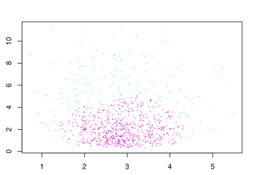
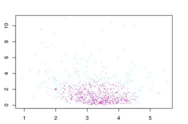
Figure 5: Two Monte-Carlo confidence regions for the parameters $\log(r)$ and $\sigma^{2}$ in the Ricker’s model, the firts (left) containing the true generating parameter, the second (right) failing in including the paramer.

5 Discussion

The Box Confidence Depth algorithm introduced in this paper provides a simple yet effective method to construct calibrated confidence intervals and regions in both likelihood-based and likelihood-free scenarios, making it versatile across various statistical contexts. The method is designed to work with multivariate parameters and potentially multivariate test statistics; in fact, it effectively uses a measure of centrality of observed data with respect to simulated data, providing intuitive ordering in multivariate spaces.

There are several areas for potential improvement. As with many Monte Carlo methods, the procedure may be demanding in terms of computational resources, especially for high-dimensional problems. To boost the computational efficiency of the method, techniques such as adaptive proposals, resampling strategies, and methods for simulating rare events may be utilized (Tokdar and Kass, 2010; Caron et al., 2014; Bugallo et al., 2017). Automated methods for selecting optimal summary statistics, even multivariate, in the absence of domain knowledge could enhance the method’s applicability. In particular, Machine Learning methods, and contrastive learning approaches can be used to learn summary statistics (see Fearnhead and Prangle, 2012; Cranmer, Pavez and Louppe, 2015; Jiang et al., 2017; Wang, Kaji and Rockova, 2022). Similarly, advanced methods for the essential density estimation step, such as Normalizing Flows (Kobyzev, Prince and Brubaker, 2020) could be adapted. A detailed exploration of these methods in this context presents an interesting direction for future research.

The first author acknowledges funding from the European Union under the ERC grant project number 864863.

References

- Azzalini and Menardi (2014) {barticle}[author] \bauthor\bsnmAzzalini, \bfnmAdelchi\binitsA. and \bauthor\bsnmMenardi, \bfnmGiovanna\binitsG. (\byear2014). \btitleClustering via nonparametric density estimation: The R package pdfCluster. \bjournalJournal of Statistical Software \bvolume57 \bpages1–26. \endbibitem
- Bernton et al. (2019) {barticle}[author] \bauthor\bsnmBernton, \bfnmEspen\binitsE., \bauthor\bsnmJacob, \bfnmPierre E\binitsP. E., \bauthor\bsnmGerber, \bfnmMathieu\binitsM. and \bauthor\bsnmRobert, \bfnmChristian P\binitsC. P. (\byear2019). \btitleApproximate Bayesian computation with the Wasserstein distance. \bjournalJournal of the Royal Statistical Society: Series B (Statistical Methodology) \bvolume81 \bpages235–269. \endbibitem
- Bugallo et al. (2017) {barticle}[author] \bauthor\bsnmBugallo, \bfnmMonica F\binitsM. F., \bauthor\bsnmElvira, \bfnmVictor\binitsV., \bauthor\bsnmMartino, \bfnmLuca\binitsL., \bauthor\bsnmLuengo, \bfnmDavid\binitsD., \bauthor\bsnmMiguez, \bfnmJoaquin\binitsJ. and \bauthor\bsnmDjuric, \bfnmPetar M\binitsP. M. (\byear2017). \btitleAdaptive importance sampling: The past, the present, and the future. \bjournalIEEE Signal Processing Magazine \bvolume34 \bpages60–79. \endbibitem
- Caron et al. (2014) {binproceedings}[author] \bauthor\bsnmCaron, \bfnmVirgile\binitsV., \bauthor\bsnmGuyader, \bfnmArnaud\binitsA., \bauthor\bsnmZuniga, \bfnmMiguel Munoz\binitsM. M. and \bauthor\bsnmTuffin, \bfnmBruno\binitsB. (\byear2014). \btitleSome recent results in rare event estimation. In \bbooktitleESAIM: Proceedings \bvolume44 \bpages239–259. \bpublisherEDP Sciences. \endbibitem
- Cranmer, Pavez and Louppe (2015) {barticle}[author] \bauthor\bsnmCranmer, \bfnmKyle\binitsK., \bauthor\bsnmPavez, \bfnmJuan\binitsJ. and \bauthor\bsnmLouppe, \bfnmGilles\binitsG. (\byear2015). \btitleApproximating likelihood ratios with calibrated discriminative classifiers. \bjournalarXiv preprint arXiv:1506.02169. \endbibitem
- Dalmasso et al. (2024) {barticle}[author] \bauthor\bsnmDalmasso, \bfnmNiccolò\binitsN., \bauthor\bsnmMasserano, \bfnmLuca\binitsL., \bauthor\bsnmZhao, \bfnmDavid\binitsD., \bauthor\bsnmIzbicki, \bfnmRafael\binitsR. and \bauthor\bsnmLee, \bfnmAnn B\binitsA. B. (\byear2024). \btitleLikelihood-free frequentist inference: Bridging classical statistics and machine learning for reliable simulator-based inference. \bjournalElectronic Journal of Statistics \bvolume18 \bpages5045–5090. \endbibitem
- Del Moral and Murray (2015) {barticle}[author] \bauthor\bsnmDel Moral, \bfnmPierre\binitsP. and \bauthor\bsnmMurray, \bfnmLawrence M\binitsL. M. (\byear2015). \btitleSequential Monte Carlo with highly informative observations. \bjournalSIAM/ASA Journal on Uncertainty Quantification \bvolume3 \bpages969–997. \endbibitem
- Efron (1979) {barticle}[author] \bauthor\bsnmEfron, \bfnmBradley\binitsB. (\byear1979). \btitleComputers and the theory of statistics: thinking the unthinkable. \bjournalSIAM review \bvolume21 \bpages460–480. \endbibitem
- Efron (2003) {barticle}[author] \bauthor\bsnmEfron, \bfnmBradley\binitsB. (\byear2003). \btitleSecond thoughts on the Bootstrap. \bjournalStatistical Science \bpages135–140. \endbibitem
- Fearnhead and Prangle (2012) {barticle}[author] \bauthor\bsnmFearnhead, \bfnmP.\binitsP. and \bauthor\bsnmPrangle, \bfnmD.\binitsD. (\byear2012). \btitleConstructing summary statistics for Approximate Bayesian computation: semi-automatic ABC (with discussion). \bjournalJournal of the Royal Statistical Society: Series B (Statistical Methodology). \endbibitem
- Frazier et al. (2018) {barticle}[author] \bauthor\bsnmFrazier, \bfnmDavid T\binitsD. T., \bauthor\bsnmMartin, \bfnmGael M\binitsG. M., \bauthor\bsnmRobert, \bfnmChristian P\binitsC. P. and \bauthor\bsnmRousseau, \bfnmJudith\binitsJ. (\byear2018). \btitleAsymptotic properties of approximate Bayesian computation. \bjournalBiometrika \bvolume105 \bpages593–607. \endbibitem
- Frazier et al. (2023) {barticle}[author] \bauthor\bsnmFrazier, \bfnmDavid T\binitsD. T., \bauthor\bsnmNott, \bfnmDavid J\binitsD. J., \bauthor\bsnmDrovandi, \bfnmChristopher\binitsC. and \bauthor\bsnmKohn, \bfnmRobert\binitsR. (\byear2023). \btitleBayesian inference using synthetic likelihood: asymptotics and adjustments. \bjournalJournal of the American Statistical Association \bvolume118 \bpages2821–2832. \endbibitem
- Gourieroux, Monfort and Renault (1993) {barticle}[author] \bauthor\bsnmGourieroux, \bfnmChristian\binitsC., \bauthor\bsnmMonfort, \bfnmAlain\binitsA. and \bauthor\bsnmRenault, \bfnmEric\binitsE. (\byear1993). \btitleIndirect inference. \bjournalJournal of Applied Econometrics \bvolume8 \bpagesS85–S118. \endbibitem
- Hermans, Begy and Louppe (2020) {binproceedings}[author] \bauthor\bsnmHermans, \bfnmJoeri\binitsJ., \bauthor\bsnmBegy, \bfnmVolodimir\binitsV. and \bauthor\bsnmLouppe, \bfnmGilles\binitsG. (\byear2020). \btitleLikelihood-free MCMC with amortized approximate ratio estimators. In \bbooktitleInternational conference on machine learning \bpages4239–4248. \bpublisherPMLR. \endbibitem
- Jiang et al. (2017) {barticle}[author] \bauthor\bsnmJiang, \bfnmBai\binitsB., \bauthor\bsnmWu, \bfnmTung-yu\binitsT.-y., \bauthor\bsnmZheng, \bfnmCharles\binitsC. and \bauthor\bsnmWong, \bfnmWing H\binitsW. H. (\byear2017). \btitleLearning summary statistic for approximate Bayesian computation via deep neural network. \bjournalStatistica Sinica \bpages1595–1618. \endbibitem
- Kenne Pagui, Salvan and Sartori (2017) {barticle}[author] \bauthor\bsnmKenne Pagui, \bfnmEuloge Clovis\binitsE. C., \bauthor\bsnmSalvan, \bfnmAlessandra\binitsA. and \bauthor\bsnmSartori, \bfnmNicola\binitsN. (\byear2017). \btitleMedian bias reduction of maximum likelihood estimates. \bjournalBiometrika \bvolume104 \bpages923–938. \endbibitem
- Kobyzev, Prince and Brubaker (2020) {barticle}[author] \bauthor\bsnmKobyzev, \bfnmIvan\binitsI., \bauthor\bsnmPrince, \bfnmSimon JD\binitsS. J. and \bauthor\bsnmBrubaker, \bfnmMarcus A\binitsM. A. (\byear2020). \btitleNormalizing flows: An introduction and review of current methods. \bjournalIEEE transactions on pattern analysis and machine intelligence \bvolume43 \bpages3964–3979. \endbibitem
- Kuchibhotla, Balakrishnan and Wasserman (2024) {barticle}[author] \bauthor\bsnmKuchibhotla, \bfnmArun Kumar\binitsA. K., \bauthor\bsnmBalakrishnan, \bfnmSivaraman\binitsS. and \bauthor\bsnmWasserman, \bfnmLarry\binitsL. (\byear2024). \btitleThe HulC: confidence regions from convex hulls. \bjournalJournal of the Royal Statistical Society Series B: Statistical Methodology \bvolume86 \bpages586–622. \endbibitem
- Laketa and Nagy (2023) {barticle}[author] \bauthor\bsnmLaketa, \bfnmPetra\binitsP. and \bauthor\bsnmNagy, \bfnmStanislav\binitsS. (\byear2023). \btitleSimplicial depth: Characterization and reconstruction. \bjournalStatistical Analysis and Data Mining: The ASA Data Science Journal \bvolume16 \bpages358–373. \endbibitem
- Liu (1990) {barticle}[author] \bauthor\bsnmLiu, \bfnmRegina Y\binitsR. Y. (\byear1990). \btitleOn a notion of Data Depth based on random simplices. \bjournalThe Annals of Statistics \bpages405–414. \endbibitem
- Liu, Liu and Xie (2022) {barticle}[author] \bauthor\bsnmLiu, \bfnmDungang\binitsD., \bauthor\bsnmLiu, \bfnmRegina Y.\binitsR. Y. and \bauthor\bsnmXie, \bfnmMin-Ge\binitsM.-G. (\byear2022). \btitleNonparametric Fusion Learning for Multiparameters: Synthesize Inferences From Diverse Sources Using Data Depth and Confidence Distribution. \bjournalJournal of the American Statistical Association \bvolume117 \bpages2086-2104. \endbibitem
- Marin et al. (2012) {barticle}[author] \bauthor\bsnmMarin, \bfnmJean-Michel\binitsJ.-M., \bauthor\bsnmPudlo, \bfnmPierre\binitsP., \bauthor\bsnmRobert, \bfnmChristian P\binitsC. P. and \bauthor\bsnmRyder, \bfnmRobin J\binitsR. J. (\byear2012). \btitleApproximate Bayesian computational methods. \bjournalStatistics and Computing \bvolume22 \bpages1167–1180. \endbibitem
- Marjoram et al. (2003) {barticle}[author] \bauthor\bsnmMarjoram, \bfnmPaul\binitsP., \bauthor\bsnmMolitor, \bfnmJohn\binitsJ., \bauthor\bsnmPlagnol, \bfnmVincent\binitsV. and \bauthor\bsnmTavaré, \bfnmSimon\binitsS. (\byear2003). \btitleMarkov chain Monte Carlo without likelihoods. \bjournalProceedings of the National Academy of Sciences \bvolume100 \bpages15324–15328. \endbibitem
- Masserano et al. (2022) {barticle}[author] \bauthor\bsnmMasserano, \bfnmLuca\binitsL., \bauthor\bsnmDorigo, \bfnmTommaso\binitsT., \bauthor\bsnmIzbicki, \bfnmRafael\binitsR., \bauthor\bsnmKuusela, \bfnmMikael\binitsM. and \bauthor\bsnmLee, \bfnmAnn B\binitsA. B. (\byear2022). \btitleSimulation-based inference with Waldo: Perfectly calibrated confidence regions using any prediction or posterior estimation algorithm. \bjournalarXiv preprint arXiv:2205.15680. \endbibitem
- Papamakarios, Sterratt and Murray (2019) {binproceedings}[author] \bauthor\bsnmPapamakarios, \bfnmGeorge\binitsG., \bauthor\bsnmSterratt, \bfnmDavid\binitsD. and \bauthor\bsnmMurray, \bfnmIain\binitsI. (\byear2019). \btitleSequential neural likelihood: Fast likelihood-free inference with autoregressive flows. In \bbooktitleThe 22nd International Conference on Artificial Intelligence and Statistics \bpages837–848. \bpublisherPMLR. \endbibitem
- Price et al. (2018) {barticle}[author] \bauthor\bsnmPrice, \bfnmLeah F\binitsL. F., \bauthor\bsnmDrovandi, \bfnmChristopher C\binitsC. C., \bauthor\bsnmLee, \bfnmAnthony\binitsA. and \bauthor\bsnmNott, \bfnmDavid J\binitsD. J. (\byear2018). \btitleBayesian Synthetic Likelihood. \bjournalJournal of Computational and Graphical Statistics \bvolume27 \bpages1–11. \endbibitem
- Pritchard et al. (1999) {barticle}[author] \bauthor\bsnmPritchard, \bfnmJ. K.\binitsJ. K., \bauthor\bsnmSeielstad, \bfnmM. T.\binitsM. T., \bauthor\bsnmPerez-Lezaun, \bfnmA.\binitsA. and \bauthor\bsnmFeldman, \bfnmM. W.\binitsM. W. (\byear1999). \btitlePopulation growth of human Y chromosomes: a study of Y chromosome microsatellites. \bjournalMolecular Biology and Evolution \bvolume16 \bpages1791. \endbibitem
- Rezende and Mohamed (2015) {binproceedings}[author] \bauthor\bsnmRezende, \bfnmDanilo\binitsD. and \bauthor\bsnmMohamed, \bfnmShakir\binitsS. (\byear2015). \btitleVariational inference with normalizing flows. In \bbooktitleInternational conference on machine learning \bpages1530–1538. \bpublisherPMLR. \endbibitem
- Ricker (1954) {barticle}[author] \bauthor\bsnmRicker, \bfnmWilliam Edwin\binitsW. E. (\byear1954). \btitleStock and recruitment. \bjournalJournal of the Fisheries Board of Canada \bvolume11 \bpages559–623. \endbibitem
- Rotiroti and Walker (2024) {barticle}[author] \bauthor\bsnmRotiroti, \bfnmFrank\binitsF. and \bauthor\bsnmWalker, \bfnmStephen G\binitsS. G. (\byear2024). \btitleApproximate Bayesian computation using the Fourier integral theorem. \bjournalElectronic Journal of Statistics \bvolume18 \bpages5156–5197. \endbibitem
- Rubin (1984) {barticle}[author] \bauthor\bsnmRubin, \bfnmDonald B\binitsD. B. (\byear1984). \btitleBayesianly justifiable and relevant frequency calculations for the applied statistician. \bjournalThe Annals of Statistics \bpages1151–1172. \endbibitem
- Schweder and Hjort (2016) {bbook}[author] \bauthor\bsnmSchweder, \bfnmTore\binitsT. and \bauthor\bsnmHjort, \bfnmNils Lid\binitsN. L. (\byear2016). \btitleConfidence, likelihood, probability \bvolume41. \bpublisherCambridge University Press. \endbibitem
- Sisson et al. (2018) {bbook}[author] \bauthor\bsnmSisson, \bfnmScott A\binitsS. A., \bauthor\bsnmFan, \bfnmYanan\binitsY., \bauthor\bsnmBeaumont, \bfnmMark\binitsM. and \bauthor\bsnmAltri (\byear2018). \btitleHandbook of Approximate Bayesian Computation. \bpublisherCRC Press. \endbibitem
- Thomas et al. (2022) {barticle}[author] \bauthor\bsnmThomas, \bfnmOwen\binitsO., \bauthor\bsnmDutta, \bfnmRitabrata\binitsR., \bauthor\bsnmCorander, \bfnmJukka\binitsJ., \bauthor\bsnmKaski, \bfnmSamuel\binitsS. and \bauthor\bsnmGutmann, \bfnmMichael U\binitsM. U. (\byear2022). \btitleLikelihood-free inference by ratio estimation. \bjournalBayesian Analysis \bvolume17 \bpages1–31. \endbibitem
- Tokdar and Kass (2010) {barticle}[author] \bauthor\bsnmTokdar, \bfnmSurya T\binitsS. T. and \bauthor\bsnmKass, \bfnmRobert E\binitsR. E. (\byear2010). \btitleImportance sampling: a review. \bjournalWiley Interdisciplinary Reviews: Computational Statistics \bvolume2 \bpages54–60. \endbibitem
- Wang, Kaji and Rockova (2022) {barticle}[author] \bauthor\bsnmWang, \bfnmYuexi\binitsY., \bauthor\bsnmKaji, \bfnmTetsuya\binitsT. and \bauthor\bsnmRockova, \bfnmVeronika\binitsV. (\byear2022). \btitleApproximate Bayesian computation via classification. \bjournalJournal of Machine Learning Research \bvolume23 \bpages1–49. \endbibitem
- Wood (2010) {barticle}[author] \bauthor\bsnmWood, \bfnmSimon N\binitsS. N. (\byear2010). \btitleStatistical inference for noisy nonlinear ecological dynamic systems. \bjournalNature \bvolume466 \bpages1102–1104. \endbibitem
- Xie and Singh (2013) {barticle}[author] \bauthor\bsnmXie, \bfnmMin-Ge\binitsM.-G. and \bauthor\bsnmSingh, \bfnmKesar\binitsK. (\byear2013). \btitleConfidence Distribution, the frequentist distribution estimator of a parameter: A review. \bjournalInternational Statistical Review \bvolume81 \bpages3–39. \endbibitem
- Xie and Wang (2022) {barticle}[author] \bauthor\bsnmXie, \bfnmMin-Ge\binitsM.-G. and \bauthor\bsnmWang, \bfnmPeng\binitsP. (\byear2022). \btitleRepro Samples Method for Finite and Large Sample Inferences. \bjournalarXiv preprint arXiv:2206.06421. \endbibitem