Generalization of the Gibbs algorithm with high probability at low temperatures

Abstract

The paper gives a bound on the generalization error of the Gibbs algorithm, which recovers known data-independent bounds for the high temperature range and extends to the low-temperature range, where generalization depends critically on the data-dependent loss-landscape. It is shown, that with high probability the generalization error of a single hypothesis drawn from the Gibbs posterior decreases with the total prior volume of all hypotheses with similar or smaller empirical error. This gives theoretical support to the belief in the benefit of flat minima. The zero temperature limit is discussed and the bound is extended to a class of similar stochastic algorithms.

1 Introduction

Controlling the difference between the empirical error and the expected future error of a hypothesis is a fundamental problem of learning theory. This paper gives high probability bounds on this generalization gap for individual hypotheses drawn from the Gibbs posterior. The Gibbs posterior assigns probabilities, which decrease exponentially with the hypothesis’ empirical error, relative to some prior reference measure. Such distributions are the minimizers of the PAC-Bayesian bound (McAllester (1999)) and limiting distributions of stochastic gradient Langevin dynamics (SGLD, Raginsky et al. (2017)). It has been argued by Zhang et al. (2018), that the popular method of stochastic gradient descent (SGD) may also be reinterpreted as a form SGLD, and is thus also related to the Gibbs-posterior. The Gibbs-algorithm, which generates the posterior from data, is therefore an important theoretical construction in the study of the generalization properties of several stochastic algorithms applied to non-convex learning tasks.

There are various known bounds, both on averages and on single hypotheses drawn from the posterior (Lever et al. (2013), Raginsky et al. (2017), Kuzborskij et al. (2019), Rivasplata et al. (2020), Aminian et al. (2021), Maurer (2024)), but most of these results become vacuous, when the inverse temperature parameter $\beta$, which governs the exponential decay of probabilities, exceeds the number $n$ of training examples. For very difficult data, or randomly permuted labels, this correctly predicts the failure of generalization. For easier data, however, generalization persists in the low temperature regime $\beta>n$. This has been experimentally observed for example by Dziugaite and Roy (2018), and nicely documented in Figure 1, Section 6 of the respective article. Any bound which retains explanatory power in the low temperature regime, must therefore be data- or distribution-dependent.

The bound given here applies with high probability to a single hypothesis drawn from the Gibbs-posterior. This is an important feature, because after the laborious processes of SGLD or SGD the final result is the draw of an individual hypothesis. The bound also predicts better generalization for the chosen hypothesis, whenever the total prior reference volume of hypotheses with similar or smaller empirical error is large, providing a partial explanation of the frequent observation, that hypotheses in wide minima generalize well (Hochreiter and Schmidhuber (1997), Keskar et al. (2016), Wu et al. (2017), Zhang et al. (2021)).

While recovering and potentially improving on existing results for the high temperature regime, our result can also guarantee generalization in the zero temperature limit $\beta\rightarrow\infty$, whenever the set of hypotheses with minimal empirical risk has positive prior measure.

Recent studies of the loss landscapes of overparametrized non-convex systems suggest, that global minimizers are generically high-dimensional manifolds (Cooper (2018), Cooper (2021), Liu et al. (2022)). We will argue heuristically, that the prior volume of the set of hypotheses close to these manifolds is necessarily small for random data, while it may be quite large for easy data, thus opening the door to successful generalization.

Following a section introducing the necessary notation and definitions the main result is stated and proved. Section 4 discusses the implications of this bound in the regimes of high and low temperature, the zero-temperature limit and the dependence on the underlying data-distribution. Section 5 gives some more concrete bounds, Section 6 extends the main result to more general stochastic algorithms, and Section 7 summarizes some related literature.

2 Preliminaries

Throughout the following $\left(\mathcal{X},\Sigma\right)$ is a measurable space of data with probability measure $\mu$. The iid random vector $\mathbf{x}\sim\mu^{n}$ is the training sample.

$\left(\mathcal{H},\Omega\right)$ is a measurable space of hypotheses, and there is a measurable loss function $\ell:\mathcal{H\times X}\rightarrow\left[0,\infty\right)$. Members of $\mathcal{H}$ are denoted $h$ or $g$. We write $L\left(h\right):=\mathbb{E}_{X\sim\mu}\left[\ell\left(h,x\right)\right]$ and $\hat{L}\left(h,\mathbf{x}\right):=\left(1/n\right)\sum_{i}\ell\left(h,x_{i}\right)$ respectively for the true (expected) and empirical loss of hypothesis $h\in\mathcal{H}$.

The set of probability measures on $\left(\mathcal{H},\Omega\right)$ is denoted $\mathcal{P}\left(\mathcal{H}\right)$. There is an a-priori reference measure $\pi\in\mathcal{P}\left(\mathcal{H}\right)$, called the prior. We write $L_{\min}=~$ess $\inf_{h\in\mathcal{H}}L\left(h\right)$ and $\hat{L}_{\min}\left(\mathbf{x}\right)=~$ess $\inf_{h\in\mathcal{H}}\hat{L}\left(h,\mathbf{x}\right)$, where the essential infimum refers to the measure $\pi$. We also write $\mathcal{H}_{\min}=\left\{h:L\left(h\right)=L_{\min}\right\}$ and $\widehat{\mathcal{H}}_{\min}\left(\mathbf{x}\right)=\left\{h:\hat{L}\left(h,\mathbf{x}\right)=\hat{L}_{\min}\left(\mathbf{x}\right)\right\}$ for the respective sets of global minimizers.

For $r\in\mathbb{R}$ we also denote with $\varphi\left(r\right)=\pi\left\{g:L\left(g\right)\leq r\right\}$ and $\hat{\varphi}\left(r,\mathbf{x}\right)=\pi\left\{g:\hat{L}\left(g,\mathbf{x}\right)\leq r\right\}$ the cumulative distribution functions of the true and empirical loss respectively.

The Gibbs algorithm at inverse temperature $\beta>0$ is the map $\hat{G}_{\beta}:\mathbf{x}\in\mathcal{X}^{n}\mapsto\hat{G}_{\beta}\left(\mathbf{x}\right)\in\mathcal{P}\left(\mathcal{H}\right)$ defined by

$$\hat{G}_{\beta}\left(\mathbf{x}\right)\left(A\right)=\frac{1}{Z_{\beta}\left(\mathbf{x}\right)}\int_{A}e^{-\beta\hat{L}\left(h,\mathbf{x}\right)}d\pi\left(h\right)\text{ for }A\in\Omega\text{.}$$

$\hat{G}_{\beta}\left(\mathbf{x}\right)$ is called the Gibbs-posterior, the normalizing factor

$$Z_{\beta}\left(\mathbf{x}\right):=\int_{\mathcal{H}}e^{-\beta\hat{L}\left(h,\mathbf{x}\right)}d\pi\left(h\right)$$

is called the partition function.

We define a probability measure $\rho$ on $\mathcal{H}\times\mathcal{X}^{n}$ by

$$\rho\left(A\right)=\mathbb{E}_{\mathbf{x}\sim\mu^{n}}\mathbb{E}_{h\sim\hat{G}_{\beta}\left(\mathbf{x}\right)}\left[1_{A}\left(h,\mathbf{x}\right)\right]\text{ for }A\in\Omega\otimes\Sigma^{\otimes n}.$$ (1)

Then $\mathbb{E}_{\left(h,\mathbf{x}\right)\sim\rho}\left[\phi\left(h,\mathbf{x}\right)\right]=\mathbb{E}_{\mathbf{x}}\mathbb{E}_{h\sim\hat{G}_{\beta}\left(\mathbf{x}\right)}\left[\phi\left(h,\mathbf{x}\right)\right]$ for measurable $\phi:\mathcal{H}\times\mathcal{X}^{n}\rightarrow\mathbb{R}$.

The relative entropy of two Bernoulli variables with expectations $p$ and $q$ is denoted

$$\kappa\left(p,q\right)=p\ln\frac{p}{q}+\left(1-p\right)\ln\frac{1-p}{1-q}.$$ (2)

Tolstikhin and Seldin (2013) give the inversion rule $\kappa\left(p,q\right)\leq B$ $\implies$ $q-p\leq\sqrt{2pB}+2B$.

3 A generic generalization bound

In applications the otherwise arbitrary function $F$ in the following theorem is a place-holder for a scalar multiple of the generalization gap.

Theorem 3.1.

Let $F:\mathcal{H}\times\mathcal{X}^{n}\rightarrow\mathbb{R}$ be some measurable function and $\delta>0$. Then with probability at least $1-\delta$ in $\mathbf{x}\sim\mu^{n}$ and $h\sim\hat{G}_{\beta}\left(\mathbf{x}\right)$

$$F\left(h,\mathbf{x}\right)\leq\inf_{r\in\mathbb{R}}\beta r+\ln\frac{1}{\hat{\varphi}\left(\hat{L}\left(h,\mathbf{x}\right)+r,\mathbf{x}\right)}+\ln\mathbb{E}_{\mathbf{x}}\mathbb{E}_{g\sim\pi}\left[e^{F\left(g,\mathbf{x}\right)}\right]+\ln\left(1/\delta\right).$$

Proof.

By Markov’s inequality (Appendix B, Lemma B.2 (i)) for any real random variable $Y$

$$\Pr\left\{Y>\ln\mathbb{E}\left[e^{Y}\right]+\ln\left(1/\delta\right)\right\}\leq\delta.$$

We apply this to the random variable $Y=F\left(h,\mathbf{x}\right)+\beta\hat{L}\left(h,\mathbf{x}\right)+\ln Z_{\beta}\left(\mathbf{x}\right)$ on the probability space $\left(\mathcal{H\times X}^{n},\Omega\otimes\Sigma^{\otimes n},\rho\right)$ as defined in (1). Together with the definition of the Gibbs-posterior this gives, with probability at least $1-\delta$ in $\left(h,\mathbf{x}\right)\sim\rho$ (equivalent to saying $\mathbf{x}\sim\mu^{n}$ and $h\sim\hat{G}_{\beta}\left(\mathbf{x}\right)$),

$$F\left(h,\mathbf{x}\right)+\beta\hat{L}\left(h,\mathbf{x}\right)+\ln Z_{\beta}\left(\mathbf{x}\right)$$

$$\leq\ln\mathbb{E}_{\mathbf{x}}\mathbb{E}_{g\sim\hat{G}_{\beta}\left(\mathbf{x}\right)}\left[e^{F\left(g,\mathbf{x}\right)+\beta\hat{L}\left(g,\mathbf{x}\right)+\ln Z_{\beta}\left(\mathbf{x}\right)}\right]+\ln\left(1/\delta\right)$$

$$=\ln\mathbb{E}_{\mathbf{x}}\mathbb{E}_{g\sim\pi}\left[e^{F\left(g,\mathbf{x}\right)+\beta\hat{L}\left(g,\mathbf{x}\right)+\ln Z_{\beta}\left(\mathbf{x}\right)-\beta\hat{L}\left(g,\mathbf{x}\right)-\ln Z_{\beta}\left(\mathbf{x}\right)}\right]+\ln\left(1/\delta\right)$$

$$=\ln\mathbb{E}_{\mathbf{x}}\mathbb{E}_{g\sim\pi}\left[e^{F\left(g,\mathbf{x}\right)}\right]+\ln\left(1/\delta\right).$$

Subtract $\beta\hat{L}\left(h,\mathbf{x}\right)+\ln Z_{\beta}\left(\mathbf{x}\right)$ to get

$$F\left(h,\mathbf{x}\right)\leq-\beta\hat{L}\left(h,\mathbf{x}\right)-\ln Z_{\beta}\left(\mathbf{x}\right)+\ln\mathbb{E}_{\mathbf{x}}\mathbb{E}_{g\sim\pi}\left[e^{F\left(g,\mathbf{x}\right)}\right]+\ln\left(1/\delta\right).$$ (3)

For any $r\in\mathbb{R}$ and $h\in\mathcal{H}$ we can lower bound the partition function by

$$Z_{\beta}\left(\mathbf{x}\right) \geq \int_{\left\{g:\hat{L}\left(g,\mathbf{x}\right)\leq\hat{L}\left(h,\mathbf{x}\right)+r\right\}}e^{-\beta\hat{L}\left(g,\mathbf{x}\right)}d\pi\left(g\right)$$

$$\geq e^{-\beta\left(\hat{L}\left(h,\mathbf{x}\right)+r\right)}\hat{\varphi}\left(\hat{L}\left(h,\mathbf{x}\right)+r,\mathbf{x}\right).$$

It follows that

$$-\beta\hat{L}\left(h,\mathbf{x}\right)-\ln Z_{\beta}\left(\mathbf{x}\right)\leq\inf_{r\in\mathbb{R}}\beta r+\ln\frac{1}{\hat{\varphi}\left(\hat{L}\left(h,\mathbf{x}\right)+r,\mathbf{x}\right)}.$$

Substitution in (3) completes the proof.

∎

The first step in the proof, the application of Markov’s inequality, produces at once a disintegrated PAC-Bayesian bound (like Theorem 1 (i) of Rivasplata et al. (2020)) as applied to the Gibbs posterior.

The second step in the proof, the lower bound on the partition function with the cumulative distribution function of the empirical loss, weakens this result, but serves the purpose of interpretability. In Section 6 this simple method is extended to other data-dependent distributions.

A similar result to Theorem 3.1 is given by Viallard et al. (2024a), with the principal difference that the parameter $r$ becomes the difference $\hat{L}\left(h^{\prime},\mathbf{x}\right)-\hat{L}\left(h,\mathbf{x}\right)$, where $h^{\prime}$ is some test hypothesis, and $\hat{\varphi}\left(\hat{L}\left(h,\mathbf{x}\right)+r,\mathbf{x}\right)$ is equated as part of the confidence parameter $\delta$ and combined with (3) in a union bound.

To simplify the statement of some corollaries we introduce the hypothesis- and data-dependent complexity measure $\Lambda_{\beta}:\mathcal{H\times X}^{n}\rightarrow\left[0,\infty\right)$

$$\Lambda_{\beta}\left(h,\mathbf{x}\right):=\inf_{r\in\mathbb{R}}\beta r+\ln\frac{1}{\hat{\varphi}\left(\hat{L}\left(h,\mathbf{x}\right)+r,\mathbf{x}\right)},$$ (4)

so the inequality in Theorem 3.1 can be written

$$F\left(h,\mathbf{x}\right)\leq\Lambda_{\beta}\left(h,\mathbf{x}\right)+\ln\mathbb{E}_{\mathbf{x}}\mathbb{E}_{g\sim\pi}\left[e^{F\left(g,\mathbf{x}\right)}\right]+\ln\left(1/\delta\right).$$ (5)

For a first application let the loss $\ell$ have values in $\left[0,1\right]$ and set $F\left(h,\mathbf{x}\right)=n~\kappa\left(\hat{L}\left(h,\mathbf{x}\right),L\left(h\right)\right)$, with $\kappa$ the relative entropy as in (2). The two expectations above can be interchanged, and from Theorem 1 of Maurer (2004) we get $\mathbb{E}_{\mathbf{x}}\left[e^{n~\kappa\left(\hat{L}\left(h,\mathbf{x}\right),L\left(h\right)\right)}\right]\leq 2\sqrt{n}$. Substitution in Theorem 3.1 and division by $n$ then give the following.

Corollary 3.2.

Assume that $\ell$ has values in $\left[0,1\right]$ and let $\delta>0$ and $n\geq 8$. Then with probability at least $1-\delta$ in $\mathbf{x}\sim\mu^{n}$ and $h\sim\hat{G}_{\beta}\left(\mathbf{x}\right)$

$$\kappa\left(\hat{L}\left(h,\mathbf{x}\right),L\left(h\right)\right)\leq\frac{1}{n}\left(\Lambda_{\beta}\left(h,\mathbf{x}\right)+\ln\left(\frac{2\sqrt{n}}{\delta}\right)\right).$$

Using the inversion rule for $\kappa$ this inequality implies

$$L\left(h\right)-\hat{L}\left(h,\mathbf{x}\right)\leq\sqrt{\frac{2\hat{L}\left(h,\mathbf{x}\right)}{n}\left(\Lambda_{\beta}\left(h,\mathbf{x}\right)+\ln\left(\frac{2\sqrt{n}}{\delta}\right)\right)}+\frac{2}{n}\left(\Lambda_{\beta}\left(h,\mathbf{x}\right)+\ln\left(\frac{2\sqrt{n}}{\delta}\right)\right).$$

Ignoring the logarithmic term this gives an approximate rate of $\Lambda_{\beta}\left(h,\mathbf{x}\right)/n$ for small $\hat{L}\left(h,\mathbf{x}\right)$.

This is not the only bound which can be derived from Theorem 3.1. Results for unbounded losses (sub-Gaussian or sub-exponential) are given in Section 5. We conclude this section with some superficial remarks on the quantity $\Lambda_{\beta}\left(h,\mathbf{x}\right)$ and Theorem 3.1.

1. Without infimum the right hand side of (4) is infinite for $r<-\hat{L}\left(h,\mathbf{x}\right)$. As $r$ ranges from $-\hat{L}\left(h,\mathbf{x}\right)$ to $+\infty$, the first term increases from $r=-\beta\hat{L}\left(h,\mathbf{x}\right)$ to $+\infty$, while the second tern is non-increasing and descends from $+\infty$ to zero. The infimum is finite and approximated (or attained) in the interval $\left(-\hat{L}\left(h,\mathbf{x}\right),+\infty\right)$.

2. $\Lambda_{\beta}\left(h,\mathbf{x}\right)$ is a random variable in its dependence on $\mathbf{x}\sim\mu^{n}$ and $h\sim\hat{G}_{\beta}\left(\mathbf{x}\right)$. It is non-increasing in $\hat{L}\left(h,\mathbf{x}\right)$, which makes some intuitive sense, since for finite $\beta$ we can sample arbitrarily large values of $\hat{L}\left(h,\mathbf{x}\right)$ within the range of the loss function. If $\hat{L}\left(h,\mathbf{x}\right)$ is larger, we expect the gap to the true loss $L\left(h\right)$ to be smaller.

3. The distributions generated by commonly used stochastic algorithms only approximate the Gibbs-posterior. Suppose we draw from an approximating sequence $\zeta_{m}\left(\mathbf{x}\right)\in\mathcal{P}\left(\mathcal{H}\right)$ instead of $\hat{G}_{\beta}\left(\mathbf{x}\right)$, and $\Delta_{\mathcal{F}}\left(\zeta_{m},\hat{G}_{\beta}\left(\mathbf{x}\right)\right)\rightarrow 0$ for some integral probability metric $\Delta_{\mathcal{F}}$ defined by some function class $\mathcal{F}$ (Definition B.1 in Appendix B). If there exists $\gamma<\infty$ such $\gamma^{-1}\exp\left(F\left(.,\mathbf{x}\right)+\beta\hat{L}\left(.,\mathbf{x}\right)\right)\in\mathcal{F}$, then we retain from Lemma B.2 (ii) (in Appendix B) that in the limit $m\rightarrow\infty$ we get the same bound on $F\left(.,\mathbf{x}\right)$ as in Theorem 3.1.

4 Interpretation of Theorem 3.1

The most important consequence of Theorem 3.1 is an at first puzzling cooperative phenomenon: generalization of a randomly chosen individual hypothesis benefits from the total prior volume of hypotheses with similar, or smaller empirical loss. The situation is depicted in Figure 1.

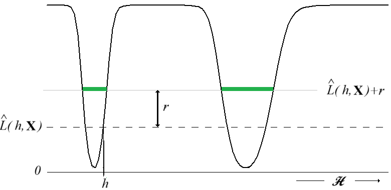
Figure 1: Schematic representation of the loss landscape, with the prior being the length of horizontal intervals. $h$ is drawn from the Gibbs-posterior and the total length of the thick green lines contributes to the prior volume and thus to generalization. Notice that for large $\beta$ and large ${\hat{L}}(h,\bf X)$ the optimal $r$ can also be negative.

4.1 Wide minima

If $\mathcal{H}$ is parametrized by $\mathbb{R}^{d}$, and the prior is given by a smooth density with respect to Lebesgue measure, then Theorem 3.1 predicts better generalization, if the near minimal hypotheses, when averaged over the prior, have larger volume. A similar observation was made by Neyshabur et al. (2017) in consequence of the PAC-Bayesian theorem. While this does not make a statement about individual minima, it still corroborates to some extent the empirically supported belief that "wide" or "flat" minima in non-convex loss landscapes are good for generalization (Hochreiter and Schmidhuber (1997), Keskar et al. (2016), Zhang et al. (2018), Dziugaite et al. (2020), Iyer et al. (2023)). The Gibbs algorithm is unlikely to sample close to narrow minima. Theorem 3.1 therefore does not make much of a statement about narrow minima, but it does make a statement about the positive cumulative effect of wide minima.

It has been argued by several authors (Dinh et al. (2017), Granziol (2020)) that reparametrizations of wide minima may become very narrow, but still compute the same function, so good generalization cannot truly be a property of wide minima. If the hypotheses are viewed in isolation, this seems a valid argument, and several authors thought of reparametrization-invariant definitions of "wideness" (see Andriushchenko et al. (2023) and references therein). From the holistic perspective of the Gibbs algorithm, however, any global reparametrization $T:\mathbb{R}^{d}\rightarrow\mathbb{R}^{d}$ must be accompanied by a corresponding push-forward of the prior $\pi\mapsto T_{\#}\left(\pi\right)$ where $T_{\#}\left(\mu\right)\left(A\right)=\pi\left(T^{-1}\left(A\right)\right)$, and in terms of the new (possibly very singular looking) prior the neighborhoods of all minima are just as wide or narrow as before the reparametrization.

4.2 High temperatures

If the loss is bounded, say $\ell\leq 1$, then setting $r=1$ instead of the infimum in (4) causes the second term to vanish, so $\Lambda\left(h,\mathbf{x}\right)\leq\beta$. Thus Corollary 3.2 guarantees the following often considerably weaker bound.

Corollary 4.1.

Assume $\ell\leq 1$ and let $n\geq 8$ and $\delta>0$. Then with probability at least $1-\delta$ in $\mathbf{x}\sim\mu^{n}$ and $h\sim\hat{G}_{\beta}\left(\mathbf{x}\right)$

$$\kappa\left(\hat{L}\left(h,\mathbf{x}\right),L\left(h\right)\right)\leq\frac{1}{n}\left(\beta+\ln\frac{2\sqrt{n}}{\delta}\right).$$

This is a data-independent worst-case bound. In the high temperature regime $\beta\ll n$ this bound is non-vacuous and comparable to the existing bounds in Lever et al. (2013), Raginsky et al. (2017), Dziugaite and Roy (2018), Kuzborskij et al. (2019), Rivasplata et al. (2020) or Maurer (2024).

4.3 Low temperatures

In the low temperature regime, when we cannot fall back on the high temperature bound of Corollary 4.1, generalization may succeed or fail in a data-dependent way, depending crucially on the cumulative distribution function of the empirical loss $\hat{\varphi}\left(r,\mathbf{x}\right)=\pi\left\{g:\hat{L}\left(g,\mathbf{x}\right)<r\right\}$.

To get an idea of the orders of magnitude involved, consider a data-set like MNIST, where we can obtain a test error as small as $10^{-2}$ from $10^{4}$ training examples. Let $\beta\approx 10^{5}$, so we are in the low-temperature regime. According to Theorem 3.1 the optimal $r^{\ast}$ must then be about $r^{\ast}\approx 10^{-3}$, but for any $\pi$ this means also that $\ln\left(1/\hat{\varphi}\left(10^{-3},\mathbf{x}\right)\right)/10^{4}\approx 10^{-2}$, equivalent to $\pi\left\{g:\hat{L}\left(g,\mathbf{x}\right)<10^{-3}\right\}\approx e^{-100}\approx 4\times 10^{-44}$. On the one hand this shows that good generalization does not make excessive demands on the prior mass of good hypotheses, which is comforting because it makes the bound seem realistic. On the other hand it also shows, that it is practically impossible to estimate $\pi\left\{g:\hat{L}\left(g,\mathbf{x}\right)<r\right\}$ by simple trials of $\pi$. This is a drawback of the proposed bound: despite the fact that it is completely data-dependent, it seems incomputable.

Corrollary 4.1 would require $\beta\approx 10^{2}$ for a generalization gap of $10^{-2}$, implying a very large training error as documented in Figure 1, Section 6 of Dziugaite and Roy (2018). The high temperature bound cannot explain this figure, while Theorem 3.1 seems to be consistent with it.

If the prior volume of the set of global empirical minimizers is positive, then, since almost surely $\hat{\varphi}\left(L\left(h,\mathbf{x}\right),\mathbf{x}\right)=\pi\left\{g:\hat{L}\left(g,\mathbf{x}\right)\leq L\left(h,\mathbf{x}\right)\right\}\geq\pi\left(\widehat{\mathcal{H}}_{\min}\left(\mathbf{x}\right)\right)$, we may set $r=0$ in (4), which yields the following.

Corollary 4.2.

If $\pi\left(\widehat{\mathcal{H}}_{\min}\left(\mathbf{x}\right)\right)>0$, then for any $\beta>0$ we have

$$\Lambda_{\beta}\left(h,\mathbf{x}\right)\leq\ln\left(1/\pi\left(\widehat{\mathcal{H}}_{\min}\left(\mathbf{x}\right)\right)\right),$$

and for $n>8$ and $\delta>0$ with probability at least $1-\delta$ in $\mathbf{x}\sim\mu^{n}$ and $h\sim\hat{G}_{\beta}\left(\mathbf{x}\right)$

$$\kappa\left(\hat{L}\left(h,\mathbf{x}\right),L\left(h\right)\right)\leq\frac{1}{n}\left(\ln\frac{1}{\pi\left(\widehat{\mathcal{H}}_{\min}\left(\mathbf{x}\right)\right)}+\ln\frac{2\sqrt{n}}{\delta}\right).$$

If $\pi\left(\widehat{\mathcal{H}}_{\min}\left(\mathbf{x}\right)\right)=0$ then beyond Theorem 3.1 and without knowledge of $\hat{\varphi}\left(r,\mathbf{x}\right)$ there is little we can say about the low temperature regime. In preparation of a heuristic discussion, we assume a polynomial growth condition.

Lemma 4.3.

Assume that there are $C,p,\alpha>0$, such that for all $r\geq 0$ we have

$$\ln\pi\left\{g:\hat{L}\left(g,\mathbf{x}\right)\leq\hat{L}_{\min}\left(\mathbf{x}\right)+r\right\}\geq\min\left\{p\ln\left(\alpha r\right)-C,0\right\}.$$ (6)

Then for $\beta>\alpha p$ and $h\in\mathcal{H}$

$$\Lambda_{\beta}\left(h,\mathbf{x}\right)\leq p\left(1+\ln\frac{\beta}{\alpha p}\right)-\beta\left(\hat{L}\left(h,\mathbf{x}\right)-\hat{L}_{\min}\left(\mathbf{x}\right)\right)+C.$$

Here $p$ is an exponent of growth and $\alpha$ a width parameter. The minimum ensures that the total prior mass is bounded by $1$.

Proof.

Write

$$\Lambda_{\beta}\left(h,\mathbf{x}\right)=\inf_{r}\beta r-\ln\pi\left\{g:\hat{L}\left(g,\mathbf{x}\right)\leq\hat{L}_{\min}\left(\mathbf{x}\right)+\left(\hat{L}\left(h,\mathbf{x}\right)-\hat{L}_{\min}\left(\mathbf{x}\right)+r\right)\right\},$$

and substitute $r=p/\beta-\left(\hat{L}\left(h,\mathbf{x}\right)-\hat{L}_{\min}\left(\mathbf{x}\right)\right)$ in the growth condition (6).

∎

Importantly $\beta$ makes an at most logarithmic positive contribution to $\Lambda$. It also makes a negative contribution, which scales linearly with the optimization error $\hat{L}\left(h,\mathbf{x}\right)-\hat{L}_{\min}\left(\mathbf{x}\right)$. If the set of minimizers has $\pi$-measure zero, the optimization error is almost surely positive for finite $\beta$. In the following discussion, however, we ignore the optimization error, and concentrate on the exponent $p$ and the parameter $C$.

Now let $\mathcal{H}$ be parametrized by $\mathbb{R}^{d}$ with Gaussian prior $\pi$ and suppose $h^{\ast}\in\mathcal{H}_{\min}\left(\mathbf{x}\right)$. If we chose $C=0$ in Lemma 4.3, the exponent of growth $p$ will be the rank of the Hessian $H$ at $h^{\ast}$. As demonstrated by Cooper (2018) (see also Cooper (2021) and Liu et al. (2022)), for a smooth and sufficiently over-parametrized loss landscape the set $\mathcal{H}_{\min}\left(\mathbf{x}\right)$ will be a (possibly disconnected) smooth manifold of codimension $n$, so the rank will be at most $n$.

If the width of the prior is not too large, larger choices of $C$ in Lemma 4.3 will allow us to use the effective rank of $H$ for $p$. For difficult data, like random labels, the effective rank will remain $n$, because the random eigenvectors will be approximately orthogonal in high dimensions. For easy data with large margins, as for example MNIST, the minimizing manifolds corresponding to examples from equal classes will be well aligned. We therefore expect the effective rank $p$ to be in the order of the number of classes, and Lemma 4.3 together with Theorem 3.1 give a good bound on the generalization gap. Giving these last two paragraphs more rigorous substance is planned for future work.

4.4 The zero-temperature limit

The next Proposition shows, that the upper bound on $\Lambda_{\beta}\left(h,\mathbf{x}\right)$ in Corollary 4.2, which does not depend on $\beta$, is in fact the limit as $\beta\rightarrow\infty$.

Proposition 4.4.

Fix $\mathbf{x}\in\mathcal{X}^{n}$. If $\pi\left(\widehat{\mathcal{H}}_{\min}\left(\mathbf{x}\right)\right)>0$ then $\Lambda_{\beta}\left(h,\mathbf{x}\right)\rightarrow\ln\left(1/\pi\left(\widehat{\mathcal{H}}_{\min}\left(\mathbf{x}\right)\right)\right)$ in probability as $\beta\rightarrow\infty$.

Proof.

We already have $\Lambda_{\beta}\left(h,\mathbf{x}\right)\leq\ln\left(1/\pi\left(\widehat{\mathcal{H}}_{\min}\left(\mathbf{x}\right)\right)\right)$. For the other direction fix $\eta,\delta>0$ and note, that by the right continuity of the distribution function there is $\epsilon$ such that for all $0<\epsilon^{\prime}\leq\epsilon$

$$\beta\epsilon^{\prime}+\ln\frac{1}{\hat{\varphi}\left(\hat{L}_{\min}\left(\mathbf{x}\right)+2\epsilon^{\prime},\mathbf{x}\right)}>\ln\left(1/\pi\left(\widehat{\mathcal{H}}_{\min}\left(\mathbf{x}\right)\right)\right)-\eta.$$ (7)

By Proposition 3.1 in Athreya and Hwang (2010) there exists $\beta_{0}$ such that $\beta>\beta_{0}$ implies that $\Pr_{h\sim\hat{G}_{\beta}\left(\mathbf{x}\right)}\left\{\hat{L}\left(h,\mathbf{x}\right)\leq\hat{L}_{\min}\left(\mathbf{x}\right)+\epsilon\right\}\geq 1-\delta$. In this event

$$\Lambda_{\beta}\left(h,\mathbf{x}\right) = \beta r^{\ast}-\ln\hat{\varphi}\left(\hat{L}\left(h,\mathbf{x}\right)+r^{\ast},\mathbf{x}\right)$$

$$\geq \beta r^{\ast}-\ln\hat{\varphi}\left(\hat{L}_{\min}\left(\mathbf{x}\right)+\epsilon+r^{\ast},\mathbf{x}\right)$$

$$\geq \beta r\left(\beta,\epsilon\right)-\ln\hat{\varphi}\left(\hat{L}_{\min}\left(\mathbf{x}\right)+\epsilon+r\left(\beta,\epsilon\right),\mathbf{x}\right),$$

where $r^{\ast}$ is the minimizer in the definition of $\Lambda$ and $r\left(\beta,\epsilon\right)$ is the minimizer of the new right hand side, which doesn’t depend on $h$ but on $\beta$ and $\epsilon$. By Corollary 4.2

$$\ln\left(1/\pi\left(\widehat{\mathcal{H}}_{\min}\left(\mathbf{x}\right)\right)\right)\geq\beta r\left(\beta,\epsilon\right)-\ln\hat{\varphi}\left(\hat{L}_{\min}\left(\mathbf{x}\right)+\epsilon+r\left(\beta,\epsilon\right),\mathbf{x}\right).$$

This implies $r\left(\beta,\epsilon\right)\leq\ln\left(1/\pi\left(\widehat{\mathcal{H}}_{\min}\left(\mathbf{x}\right)\right)\right)/\beta$, so by making $\beta$ large enough we can ensure that $r\left(\beta,\epsilon\right)<\epsilon$, so (7) implies $\Lambda\left(h,\mathbf{x}\right)\geq\ln\left(1/\pi\left(\widehat{\mathcal{H}}_{\min}\left(\mathbf{x}\right)\right)\right)-\eta$. ∎

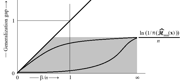
Figure 2: Schematic and compactified phase diagram of the bounds when $\pi(\widehat{\mathcal{H}}_{\min}\left(\mathbf{x}\right))>0$ with $n$ fixed. The diagonal represents the data-independent bounds of Corollary 4.1. The data-dependent bounds have to lie in the shaded region by Corollary 4.2 and converge to $\ln\left(1/\pi\left(\widehat{\mathcal{H}}_{\min}\left(\mathbf{x}\right)\right)\right)/n$ by Proposition 4.4, ignoring smaller logarithmic terms.

As an example let $\mathcal{H}$ be finite, with $\pi$ being the uniform counting measure and consider the Gibbs-algorithm in the low temperature limit $\beta\rightarrow\infty$, where the posterior becomes uniform on the set of minimizers (see Athreya and Hwang (2010)). If there is only a single minimizer then $\pi\left(\widehat{\mathcal{H}}_{\min}\left(\mathbf{x}\right)\right)=1/\left|\mathcal{H}\right|$ and the bound becomes one of roughly order $\ln\left(\left|\mathcal{H}\right|\right)/n$, which is just the usual bound, serving as a sanity check. But if there are $K$ minimizers we get an additional term of $-\ln K/n$, decreasing the generalization gap, another instance of cooperative behavior. A similar phenomenon is predicted by the Pac-Bayesian bound, but here we are not considering a posterior average, but the draw of single hypothesis.

The consequences of Corollaries 4.1, 4.2 and Proposition 4.4 are summarized in Figure 2.

4.5 Distribution-dependence and reproducibility

With $\mathcal{H}$ and $\pi$ fixed generalization of the Gibbs algorithm should be a property of the underlying data distribution $\mu$. We expect that for new data drawn from $\mu^{n}$ similar results should be obtained. Since the bound in Theorem 3.1 depends essentially on the cumulative distribution function of the empirical loss $\hat{\varphi}\left(r,\mathbf{x}\right)=\pi\left\{h:\hat{L}\left(h,\mathbf{x}\right)>r\right\}$, this function should in some sense concentrate on its distribution dependent counterpart $\varphi\left(r\right)=\pi\left\{h:L\left(h\right)>r\right\}$. Such is the content of the following proposition, which may be of independent interest.

Proposition 4.5.

Let $\delta>0$ and $p\in\mathbb{N}$. Set

$$s\left(n,\delta,p\right):=\sqrt{\frac{\ln\left(\left(1+n^{2p+1}\right)/\delta\right)}{2n}}.$$

(i) With probability at least $1-\delta$ in $\mathbf{x}\sim\mu^{n}$ we have for all $r\in\mathbb{R}$ that

$$\hat{\varphi}\left(r+s\left(n,\delta,p\right),\mathbf{x}\right)\geq\varphi\left(r\right)-n^{-p}s\left(n,\delta,p\right).$$

(ii) With probability at least $1-\delta$ in $\mathbf{x}\sim\mu^{n}$ we have for all $r\in\mathbb{R}$ that

$$\varphi\left(r+s\left(n,\delta,p\right)\right)\geq\hat{\varphi}\left(r,\mathbf{x}\right)-n^{-p}s\left(n,\delta,p\right).$$

We allow a shift within the cumulative distribution functions of $O\left(\left(p\ln n\right)/n\right)$ but a shift of the measures smaller by a factor of $n^{-p}$, where we can choose $p$. This is because of the magnitudes of numbers we expect. In the numerical example in Section 4.3 we had $r\approx 10^{-3}$, but $\hat{\varphi}\left(r,\mathbf{x}\right)=\pi\left\{g:\hat{L}\left(g,\mathbf{x}\right)\leq r\right\}\approx 10^{-44}$.

The proof (detailed in Appendix C) first reduces the inequality in (i) to a bound on the probability $\mu^{n}\left\{\mathbf{x}:\pi\left\{h:\hat{L}\left(h,\mathbf{x}\right)-L\left(h\right)>s\right\}>t\right\}$. This is then bounded by approximating $\pi$ with $\left(1+n^{2p+1}\right)$ trials, for each trial $h_{k}\sim\pi$ estimating $\mu^{n}\left\{\hat{L}\left(h_{k},\mathbf{x}\right)-L\left(h_{k}\right)>s\right\}$ with Hoeffding’s inequality and concluding with a union bound over the trials.

For difficult or impossible tasks, such as randomly permuted labels, $L_{\min}=~$ess$~\inf_{h\in\mathcal{H}}L\left(h\right)$ is large, and $\varphi\left(r\right)=0$ for $r<L_{\min}$. But for overparametrized $\mathcal{H}$ and large $\beta$ it may yet happen that $\hat{L}_{\min}\left(\mathbf{x}\right)$ is small or even zero. Proposition 4.5 (ii) then still guarantees with high probability

$$\hat{\varphi}\left(L_{\min}-t\left(n,\delta\right),\mathbf{x}\right)\leq n^{-p}s\left(n,\delta,p\right),$$

so for randomly permuted labels the total prior volume of hypotheses with small empirical error is necessarily small and decreases with the sample size, regardless of the fact that we can find small minima of the empirical error. In this sense Theorem 3.1 and Proposition 4.5 predict narrow minima for random labels. Figures 7 and 8 in Zhang et al. (2018) illustrate this point.

With Proposition 4.5 (i) at hand a union bound gives the following corollary of Theorem 3.1.

Corollary 4.6.

Let $F$ be a measurable function on $\mathcal{H}\times\mathcal{X}^{n}$. For $\delta>0$ and $p\in\mathbb{N}$ and $\left(h,\mathbf{x}\right)\in\mathcal{H}\times\mathcal{X}^{n}$ let

$$S\left(h,\mathbf{x}\right)=\left\{r:{\varphi}\left(\hat{L}\left(h,\mathbf{x}\right)+r-s\left(n,\delta,p\right)\right)-n^{-p}s\left(n,\delta,p\right)>0\right\}.$$

Then with probability at least $1-\delta$ as $\mathbf{x}\sim\mu^{n}$

$$F\left(h,\mathbf{x}\right) \leq \inf_{r\in S\left(h,\mathbf{x}\right)}\beta r+\ln\frac{1}{{\varphi}\left(\hat{L}\left(h,\mathbf{x}\right)+r-s\left(n,\delta,p\right)\right)-n^{-p}s\left(n,\delta,p\right)}$$

$$+\ln E_{\mathbf{x}}E_{h\sim\pi}\left[e^{F\left(h,\mathbf{x}\right)}\right]+\ln\left(2/\delta\right).$$

The fact that Proposition 4.5 allows a shift of $O\left(\sqrt{\left(p\ln n\right)/n}\right)$ makes the distribution-dependent bound above somewhat loose for the important small values of $r$.

5 Other corollaries of Theorem 3.1

The freedom in the choice of $F$ allows a number of bounds to be derived from Theorem 3.1. A real random variable $Y$ is $\sigma$-sub-Gaussian if $\ln\mathbb{E}e^{\lambda Y-\mathbb{E}Y}\leq\lambda^{2}\sigma^{2}/2$ for all $\lambda\in\mathbb{R}$. Now suppose all the $x\in\mathcal{X\mapsto\ell}\left(h,x\right)$ are $\sigma$-sub-Gaussian as $x\sim\mu$. Then $\mathbf{x}\in\mathcal{X}^{n}\mapsto\hat{L}\left(h,\mathbf{x}\right)$ as $\mathbf{x}\sim\mu^{n}$ is $\sigma/\sqrt{n}$-sub-Gaussian. It is tempting to set $F=\lambda\left(L\left(h\right)-\hat{L}\left(h,\mathbf{x}\right)\right)$ in Theorem 3.1, divide by $\lambda$ and then optimize over $\lambda$. Unfortunately the last step is impossible, since the optimal $\lambda$ is data-dependent in its dependence on $\Lambda$ and ruins the exponential moment bound on $F$. A more careful argument given in Appendix D stratifies the values of $\Lambda$ and establishes the following.

Corollary 5.1.

Suppose that for all $h\in\mathcal{H}$ the random variables $x\in\mathcal{X\mapsto\ell}\left(h,x\right)$ as $x\sim\mu$ are $\sigma$-sub-Gaussian. Then for $\delta>0$ with probability at least $1-\delta$ as $\left(h,\mathbf{x}\right)\sim\rho$

$$\left|L\left(h\right)-\hat{L}\left(h,\mathbf{x}\right)\right|\leq 2\sigma\sqrt{\frac{\max\left\{\Lambda_{\beta}\left(h,\mathbf{x}\right),1\right\}+\ln\left(2\Lambda_{\beta}\left(h,\mathbf{x}\right)/\delta\right)/2}{n}}.$$

Similar techniques lead to bounds for sub-exponential losses. Here we only give a weak bound with the following direct and crude argument. Set $F\left(h,\mathbf{x}\right)=\sqrt{n}\left(L\left(h\right)-\hat{L}\left(h,\mathbf{x}\right)\right)$ and use Proposition 2.7.1 and (2.24) in Vershynin (2018) with $\lambda=\sqrt{n}$ to obtain the following.

Corollary 5.2.

If $\delta>0$ then there exist absolute constants $c_{1}$ and $c_{2}$ such that for $\sqrt{n}\geq c_{2}\sup_{g\in\mathcal{H}}\left\|Y_{g}\right\|_{\psi_{1}}$ and $\delta>0$ with probability at least $1-\delta$ as $X\sim\mu^{n}$ and $h\sim\hat{G}_{\beta}\left(\mathbf{x}\right)$

$$L\left(h\right)-\hat{L}\left(h,\mathbf{x}\right)\leq\frac{\Lambda_{\beta}\left(h,\mathbf{x}\right)+c_{1}\sup_{g\in\mathcal{H}}\left\|Y_{g}\right\|_{\psi_{1}}+\ln\left(1/\delta\right)}{\sqrt{n}},$$

where $Y_{g}$ is the random variable $x\in\mathcal{X\mapsto\ell}\left(g,x\right)$ as $x\sim\mu$.

The quantity $\Lambda_{\beta}\left(h,\mathbf{x}\right)$ is oblivious to the nature of the random variable $\mathbf{x}$, so any method to bound $\ln\mathbb{E}_{\mathbf{x}}e^{\lambda\left(L\left(h\right)-\hat{L}\left(h,\mathbf{x}\right)\right)}$ can be used to derive bounds from Theorem 3.1, as long as either $\lambda$ is fixed beforehand ($\sqrt{n}$ seems always a good choice), or special care is taken as in the proof of Corollary 5.1, which leads to an additional logarithmic term in $\Lambda_{\beta}\left(h,\mathbf{x}\right)$. In this way we obtain bounds also for martingales or complicated nonlinear functions of the data, whose exponential moments can be controlled.

Theorem 3.1 highlights the benefit of a well aligned prior reference distribution $\pi$. Since the bound is data-dependent this suggests the use of a data-dependent prior $\pi\left(\mathbf{x}\right)$. Then the expectations in $\ln\mathbb{E}_{\mathbf{x}}\mathbb{E}_{h\sim\pi\left(\mathbf{x}\right)}\left[e^{F\left(h,\mathbf{X}\right)}\right]$ cannot be exchanged, and the situation becomes more complicated. But several solutions are given in Dziugaite and Roy (2018), Rivasplata et al. (2020) and Maurer (2024). Bounds on $\ln\mathbb{E}_{\mathbf{X}}\mathbb{E}_{h\sim\pi\left(\mathbf{x}\right)}\left[e^{F\left(h,\mathbf{X}\right)}\right]$ exist and can be substituted in Theorem 3.1, for example when the prior is given by Gaussian randomization of a stable algorithm as described in Section 4 of the last reference above.

6 Beyond the Gibbs algorithm

Theorem3.1 can be extended to other stochastic algorithms, if they produce densities, which are non-increasing functions of the empirical loss, satisfying a logarithmic Lipschitz condition.

Theorem 6.1.

Suppose that there is a measurable function $q:\left[0,\infty\right)\times\mathcal{X}^{n}\rightarrow\left[0,\infty\right)$ such that for every $\mathbf{x}\in\mathcal{X}^{n}$

(i) $\int_{\mathcal{H}}q\left(\hat{L}\left(h,\mathbf{x}\right),\mathbf{x}\right)d\pi\left(h\right)=1$.

(ii) $q\left(t,\mathbf{x}\right)$ is non-increasing in $t\in\left[0,\infty\right)$.

(iii) $\ln q\left(t,\mathbf{x}\right)-\ln q\left(s,\mathbf{x}\right)\leq\gamma\left(\mathbf{x}\right)\left|t-s\right|$ for $s,t\in\left[0,\infty\right)$.

Let $Q\left(\mathbf{x}\right)$ be the measure on $\Omega$ defined by $Q\left(\mathbf{x}\right)\left(A\right)=\int_{A}q\left(\hat{L}\left(h,\mathbf{x}\right),\mathbf{x}\right)d\pi\left(h\right)$. Then $Q\left(\mathbf{x}\right)\in\mathcal{P}\left(\mathcal{H}\right)$ and for $F$ as in Theorem 3.1 and $\delta>0$ with probability at least $1-\delta$ as $x\sim\mu^{n}$ and $h\sim Q\left(\mathbf{x}\right)$

$$F\left(h,\mathbf{x}\right)\leq\Lambda_{\gamma\left(\mathbf{x}\right)}\left(h,\mathbf{x}\right)+\ln\mathbb{E}_{\mathbf{x}}\mathbb{E}_{g\sim\pi}\left[e^{F\left(g,\mathbf{x}\right)}\right]+\ln\left(1/\delta\right).$$

The Gibbs algorithm satisfies the conditions of the theorem with $\gamma\left(\mathbf{x}\right)=\beta$. One conclusion is that Theorem 3.1 also holds with data-dependent temperature, but Theorem 6.1 gives much greater freedom in the choice of posteriors. The proof, detailed in Appendix E, is similar to the proof of Theorem 3.1.

7 Related work

The Gibbs algorithm traces its origin to the work of Boltzmann (1877) and Gibbs (1902) on statistical mechanics, and its relevance to machine learning was recognized by Levin et al. (1990) and Opper and Haussler (1991). McAllester (1999) realized that the minimizers of the PAC-Bayesian bound are Gibbs distributions. The fact that they are limiting distributions of stochastic gradient Langevin dynamics (Raginsky et al. (2017)), raises the question about the generalization properties of individual hypotheses as addressed in this paper. Average generalization of the Gibbs posterior was further studied notably by Aminian et al. (2021) and Aminian et al. (2023), where there are also investigations into the limiting behavior as $\beta\rightarrow\infty$.

Theorem 3.1 is part of the circle of information theoretic ideas in machine learning, ranging from the PAC-Bayesian theorem (Shawe-Taylor and Williamson (1997), McAllester (1999), McAllester (2003), Catoni (2003)) to generalization bounds in terms of mutual information (Russo and Zou (2016) and Xu and Raginsky (2017)). It is inspired by and indebted to the disintegrated PAC-Bayesian bounds as in Blanchard and Fleuret (2007), Rivasplata et al. (2020) and Viallard et al. (2024b).

The benefit of wide minima was noted by Hochreiter and Schmidhuber (1997), where also a variant of the Gibbs algorithm was discussed. The idea was promoted by Keskar et al. (2016) and others Zhang et al. (2018), Iyer et al. (2023). It was soon objected by Dinh et al. (2017) that there are narrow reparametrizations of wide minima which compute the same function. Several authors then searched for reparametrization-invariant measures of "width" (Andriushchenko et al. (2023), Kristiadi et al. (2024)). Nevertheless it was early conjectured (Neyshabur et al. (2017)), that the relevant property is average width, which is also the position of the paper at hand.

8 Conclusion

This paper does not claim to solve the mystery of generalization for deep neural networks. Even if the hand-waving discussion at the end of Section 4.3 was made rigorous, even if it produced quantitatively correct predictions, it would still not give a clue, how a deterministic algorithm, such as simple gradient descent, can produce hypotheses, which generalize well in overparametrized systems.

Theorem 3.1 is hinged on the stochastic nature of the Gibbs algorithm, and there it seems to give a plausible qualitative idea of the conditions under which generalization is possible.

A second disclaimer regards novelty. Most conclusions in this paper have counterparts, which could have been derived from the PAC-Bayesian theorem, with the principal difference that then they would be concerned with posterior averages instead of individual hypotheses. But even the disintegrated bounds are not new, but given in Rivasplata et al. (2020) or Viallard et al. (2024a).

The principal contributions of this paper are the application to the Gibbs algorithm and the lower bound on the partition function, which exposes the connection between generalization and the cumulative distribution function of the empirical loss.

Apart from tying up the various loose ends, the most important future work is to find a way to obtain quantitative confirmation of the qualitative predictions made by the paper.

Appendix A Table of notation

, $\mathcal{X}$ space of data $\mu$ probability of data $n$ sample size $\mathbf{x}$ generic member $\left(x_{1},...,x_{n}\right)\in\mathcal{X}^{n}$ $\mathbf{x}$ training set $\mathbf{x}=\left(X_{1},...,X_{n}\right)\sim\mu^{n}$ $\mathcal{H}$ hypothesis space$:\mathcal{X\rightarrow}\left[0,\infty\right)$) $h,g$ members of $\mathcal{H}$ $\ell$ loss function $\ell:\mathcal{H\times X}\rightarrow\left[0,\infty\right)$ $h\left(x\right),g\left(x\right)$ shorthand for $\ell\left(h,x\right),\ell\left(g,x\right)$ $\mathcal{P}\left(\mathcal{H}\right)$ probability measures on $\mathcal{H}$ $\pi$ prior reference measure on $\mathcal{H}$ $L\left(h\right)$ $L\left(h\right)=\mathbb{E}_{x\sim\mu}\left[h\left(x\right)\right]=\mathbb{E}_{x\sim\mu}\left[\ell\left(h,x\right)\right]$, expected (true) risk of $h\in\mathcal{H}$ $\hat{L}\left(h,\mathbf{x}\right)$ $\hat{L}\left(h,\mathbf{x}\right)=\left(1/n\right)\sum_{i=1}^{n}h\left(X_{i}\right)=\left(1/n\right)\sum_{i=1}^{n}\ell\left(h,X_{i}\right)$, empirical risk of $h\in\mathcal{H}$ $L_{\min}$ $L_{\min}=$ ess$~\inf_{h\in\mathcal{H}}L\left(h\right)$, global risk minimum $\hat{L}_{\min}\left(\mathbf{x}\right)$ $\hat{L}_{\min}\left(\mathbf{x}\right)=$ ess$~\inf_{h\in\mathcal{H}}L\left(h,\mathbf{x}\right)$, global empirical risk minimum $\mathcal{H}_{\min}$ $\mathcal{H}_{\min}=\left\{h:L\left(h\right)=L_{\min}\right\}$, set of risk minimizers $\widehat{\mathcal{H}}_{\min}\left(\mathbf{x}\right)$ $\widehat{\mathcal{H}}_{\min}\left(\mathbf{x}\right)=\left\{h:L\left(h,\mathbf{x}\right)=\hat{L}_{\min}\left(\mathbf{x}\right)\right\}$, set of empirical risk minimizers $\varphi\left(r\right)$ $\varphi\left(r\right)=\pi\left\{g:L\left(g\right)\leq r\right\}$, cumulative distribution function of true loss $\hat{\varphi}\left(r,\mathbf{x}\right)$ $\hat{\varphi}\left(r,\mathbf{x}\right)=\pi\left\{g:\hat{L}\left(g,\mathbf{x}\right)\leq r\right\}$, cumulative distribution function of empirical loss $\beta$ inverse temperature $Z_{\beta}\left(\mathbf{x}\right)$ $Z_{\beta}\left(\mathbf{x}\right)=\int_{\mathcal{H}}e^{-\beta\hat{L}\left(h,\mathbf{x}\right)}d\pi\left(h\right)$, partition function $\hat{G}_{\beta}\left(\mathbf{x}\right)$ $\hat{G}_{\beta}\left(\mathbf{x}\right)=Z_{\beta}\left(\mathbf{x}\right)^{-1}e^{-\beta\hat{L}\left(h,\mathbf{x}\right)}d\pi\left(h\right)$, Gibbs posterior $\rho$ $\rho\left(A\right)=\mathbb{E}_{\mathbf{x}}\mathbb{E}_{h\sim\hat{G}_{\beta}\left(\mathbf{x}\right)}\left[1_{A}\left(h,\mathbf{x}\right)\right]$, joint distribution of $\mathbf{x}$ and $\hat{G}_{\beta}\left(\mathbf{x}\right)$ on $\mathcal{H\times X}^{n}$ $\Lambda_{\beta}\left(h,\mathbf{x}\right)$ $\Lambda_{\beta}\left(h,\mathbf{x}\right)=\inf_{r\in\mathbb{R}}\beta r+\ln\frac{1}{\pi\left\{g:\hat{L}\left(g,\mathbf{x}\right)\leq\hat{L}\left(h,\mathbf{x}\right)+r\right\}}$, complexity measure $\kappa$ $\kappa\left(p,q\right)=p\ln\frac{p}{q}+\left(1-p\right)\ln\frac{1-p}{1-q}$, relative entropy of $p$- and $q$-Bernoulli variables $\left|A\right|$ cardinality of set $1_{A}$ indicator function of set $\left\|.\right\|_{\psi_{2}}$ sub-Gaussian norm (see Sec. 2.5.2 in Vershynin [2018]) $\left\|.\right\|_{\psi_{1}}$ sub-exponential norm (see Sec. 2.7 in Vershynin [2018])

Appendix B Markov’s inequality and integral probability metrics

Definition B.1.

Let $\left(\mathcal{Y},\Xi\right)$ be a measurable space. If $\mathcal{F}$ is a set of measurable real valued functions on $\left(\mathcal{Y},\Xi\right)$ the integral probability metric is the metric $\Delta_{\mathcal{F}}$ on $\mathcal{P}\left(\mathcal{Y}\right)$ defined by

$$\Delta_{\mathcal{F}}\left(\zeta,\xi\right)=\sup_{f\in\mathcal{F}}\left|\mathbb{E}_{y\sim\zeta}f\left(y\right)-\mathbb{E}_{y\sim\xi}f\left(y\right)\right|.$$

Lemma B.2.

(i) Let $Y$ be real random variable and $\delta>0$. Then

$$\Pr\left\{Y>\ln\mathbb{E}\left[e^{Y}\right]+\ln\left(1/\delta\right)\right\}<\delta.$$

(ii) Let $f$ be a measurable real function on $\left(\mathcal{Y},\Xi\right)$, $\mathcal{F}$ ia set of measurable real valued functions on $\left(\mathcal{Y},\Xi\right)$ and $\zeta$,$\xi\in\mathcal{P}\left(\mathcal{Y}\right)$. Then

$$\Pr_{y\sim\zeta}\left\{f\left(y\right)>\ln\mathbb{E}_{y\sim\xi}\left[e^{f\left(y\right)}\right]+\sup\left\{\gamma:\frac{e^{f\left(y\right)}}{\gamma}\in\mathcal{F}\right\}\Delta_{\mathcal{F}}\left(\zeta,\xi\right)+\ln\left(1/\delta\right)\right\}.$$

Proof.

(i) $\Pr\left\{Y>\ln\mathbb{E}\left[e^{Y}\right]+\ln\left(1/\delta\right)\right\}=\Pr\left\{e^{Y}>\frac{\mathbb{E}\left[e^{Y}\right]}{\delta}\right\}<\frac{\mathbb{E}\left[e^{Y}\right]}{\mathbb{E}\left[e^{Y}\right]/\delta}=\delta$, where the inequality is just Markov’s inequality in its usual form. ∎

(ii) We have

$$\mathbb{E}_{y\sim\zeta}\left[e^{f\left(y\right)}\right]\leq\mathbb{E}_{y\sim\xi}\left[e^{f\left(y\right)}\right]+\sup\left\{\gamma:\frac{e^{f\left(y\right)}}{\gamma}\in\mathcal{F}\right\}\Delta_{\mathcal{F}}\left(\zeta,\xi\right).$$

Using $\ln\left(a+b\right)\leq\ln a+\frac{b}{a}$ for $a,b>0$ we get

$$\ln\mathbb{E}_{y\sim\zeta}\left[e^{f\left(y\right)}\right]\leq\ln\mathbb{E}_{y\sim\xi}\left[e^{f\left(y\right)}\right]+\frac{\sup\left\{\gamma:\frac{e^{f\left(y\right)}}{\gamma}\in\mathcal{F}\right\}}{\mathbb{E}_{y\sim\xi}\left[e^{f\left(y\right)}\right]}\Delta_{\mathcal{F}}\left(\zeta,\xi\right).$$

Then use (i).

Appendix C Proof of Proposition 4.5

Proposition C.1 (Restatement of Proposition 4.5).

Let $\delta>0$ and $p\in\mathbb{N}$. Set

$$s\left(n,\delta,p\right):=\sqrt{\frac{\ln\left(\left(1+n^{2p+1}\right)/\delta\right)}{2n}}.$$

(i) With probability at least $1-\delta$ in $\mathbf{x}\sim\mu^{n}$ we have for all $r\in\mathbb{R}$ that

$$\hat{\varphi}\left(r+s\left(n,\delta,p\right),\mathbf{x}\right)\geq\varphi\left(r\right)-n^{-p}s\left(n,\delta,p\right).$$

(ii) With probability at least $1-\delta$ in $\mathbf{x}\sim\mu^{n}$ we have for all $r\in\mathbb{R}$ that

$$\varphi\left(r+s\left(n,\delta,p\right)\right)\geq\hat{\varphi}\left(r,\mathbf{x}\right)-n^{-p}s\left(n,\delta,p\right).$$

Proof.

Let $s,t>0$. Then, writing out the probability measure on $\mathcal{X}^{n}$ as $\mu^{n}$, we have for all $r\in\mathbb{R}$

$$\Pr_{\mathbf{x}\sim\mu^{n}}\left\{\hat{\varphi}\left(r+s,\mathbf{x}\right)<\varphi\left(r\right)-t\right\}$$

$$=\mu^{n}\left\{\mathbf{x}:\pi\left\{h:\hat{L}\left(h,\mathbf{x}\right)\leq r+s\right\}<\pi\left\{L\left(h\right)\leq r\right\}-t\right\}$$

$$\leq\mu^{n}\left\{\mathbf{x}:\pi\left\{h:\hat{L}\left(h,\mathbf{x}\right)\leq r+s\wedge L\left(h\right)\leq r\right\}<\pi\left\{L\left(h\right)<r\right\}-t\right\}$$

$$=\mu^{n}\left\{\mathbf{x}:\pi\left\{L\left(h\right)\leq r\right\}-\pi\left\{h:\hat{L}\left(h,\mathbf{x}\right)>r+s\wedge L\left(h\right)\leq r\right\}<\pi\left\{L\left(h\right)\leq r\right\}-t\right\}$$

$$=\mu^{n}\left\{\mathbf{x}:\pi\left\{h:\hat{L}\left(h,\mathbf{x}\right)>r+s\wedge L\left(h\right)\leq r\right\}>t\right\}$$

$$\leq\mu^{n}\left\{\mathbf{x}:\pi\left\{h:\hat{L}\left(h,\mathbf{x}\right)-L\left(h\right)>s\right\}>t\right\}.$$

Note that $r$ has disappeared from the last expression. Now let $K\in\mathbb{N}$ and use the fact that $\pi$ is a probability measure and introduce an iid $K$-sample of hypotheses $\mathbf{h}\sim\pi^{K}$ to approximate $\pi$.

$$\mu^{n}\left\{\mathbf{x}:\pi\left\{h:\hat{L}\left(h,\mathbf{x}\right)-L\left(h\right)>s\right\}>t\right\}$$

$$=\pi^{K}\times\mu^{n}\left\{\left(\mathbf{h},\mathbf{x}\right):\pi\left\{h:\hat{L}\left(h,\mathbf{x}\right)-L\left(h\right)>s\right\}>t\right\}$$

$$\leq\pi^{K}\times\mu^{n}\left\{\left(\mathbf{h},\mathbf{x}\right):\pi\left\{h:\hat{L}\left(h,\mathbf{x}\right)-L\left(h\right)>s\right\}-\frac{1}{K}\left|\left\{k:\hat{L}\left(h_{k},\mathbf{x}\right)-L\left(h_{k}\right)>s\right\}\right|>t\right\}$$

$$+\pi^{K}\times\mu^{n}\left\{\left(\mathbf{h},\mathbf{x}\right):\frac{1}{K}\left|\left\{k:\hat{L}\left(h_{k},\mathbf{x}\right)-L\left(h_{k}\right)>s\right\}\right|>0\right\}$$

$$\leq e^{-2Kt^{2}}+Ke^{-2ns^{2}}.$$

The first inequality is a union bound. Then the first probability is bounded with Hoeffding’s inequality applied to $\mathbf{h}$, which gives $e^{-Kt^{2}}$. The event in the second probability is contained in the union of $K$ events $\left\{\hat{L}\left(h_{k},\mathbf{x}\right)-L\left(h_{k}\right)>s\right\}$ and is bounded by $Ke^{-2ns^{2}}$ using Hoeffding’s inequality applied to $\mathbf{x}$ in combination with a union bound. The argument depends crucially on the independence of $\mu$ and $\pi$. Combining the previous two displays gives

$$\Pr_{\mathbf{x}}\left\{\pi\left\{h:\hat{L}\left(h,\mathbf{x}\right)\leq r+s\right\}<\pi\left\{L\left(h\right)\leq r\right\}-t\right\}\leq e^{-2Kt^{2}}+Ke^{-2ns^{2}}.$$

Now we set $K=n^{2p+1}$, and set $t=n^{-p}s$. Then the probability above becomes $\left(1+n^{2p+1}\right)e^{-2ns^{2}}$ and equating it to $\delta$ and solving for $s$ gives $s=s\left(n,\delta,p\right)$ and $t=n^{-p}s\left(n,\delta,p\right)$. This completes the proof of (i). Exchanging the roles of $L\left(h\right)$ and $\hat{L}\left(h,\mathbf{x}\right)$ in this argument gives (ii). ∎

Appendix D Proof of Corollary 5.1

We reproduce Lemma 15.6 in Anthony and Bartlett [1999].

Lemma D.1.

(Lemma 15.6 in Anthony and Bartlett [1999]) Suppose $\Pr$ is a probability distribution and

$$\left\{E\left(\alpha_{1},\alpha_{2},\delta\right):0<\alpha_{1},\alpha_{2},\delta\leq 1\right\}$$

is a set of events, such that

(i) For all $0<\alpha\leq 1$ and $0<\delta\leq 1$,

$$\Pr\left\{E\left(\alpha,\alpha,\delta\right)\right\}\leq\delta.$$

(ii) For all $0<\alpha_{1}\leq\alpha\leq\alpha_{2}\leq 1$ and $0<\delta_{1}\leq\delta\leq 1$

$$E\left(\alpha_{1},\alpha_{2},\delta_{1}\right)\subseteq E\left(\alpha,\alpha,\delta\right).$$

Then for $0<a,\delta<1$,

$$\Pr\bigcup_{\alpha\in\left(0,1\right]}E\left(\alpha a,\alpha,\delta\alpha\left(1-a\right)\right)\leq\delta.$$

Proof of Corollary 5.1.

By a standard subgaussian bound for iid random variables we have

$$\ln\mathbb{E}_{\mathbf{x}}\mathbb{E}_{h\sim\pi}\left[e^{\lambda\left(L\left(h\right)-\hat{L}\left(h,\mathbf{x}\right)\right)}\right]=\ln\mathbb{E}_{h\sim\pi}\mathbb{E}_{\mathbf{x}}\left[e^{\lambda\left(L\left(h\right)-\hat{L}\left(h,\mathbf{x}\right)\right)}\right]\leq\frac{\lambda^{2}\sigma^{2}}{2n}.$$

For any $\alpha\in\left(0,1\right]$ set $\lambda\left(\alpha\right)=\sqrt{2n\left(\alpha^{-1}+\ln\left(1/\delta\right)\right)}/\sigma$ and define the event

$$E\left(\alpha_{1},\alpha_{2},\delta\right) = \left\{\Lambda\left(h,\mathbf{x}\right)\leq\alpha_{2}^{-1}\wedge\lambda\left(\alpha_{1}\right)\left(L\left(h\right)-\hat{L}\left(h,\mathbf{x}\right)\right)>\alpha_{1}^{-1}+\frac{\lambda\left(\alpha_{1}\right)^{2}\sigma^{2}}{2n}+\ln\left(1/\delta\right)\right\}$$

$$= \left\{\Lambda\left(h,\mathbf{x}\right)\leq\alpha_{2}^{-1}\wedge L\left(h\right)-\hat{L}\left(h,\mathbf{x}\right)>\sigma\sqrt{2\left(\frac{\alpha_{1}^{-1}+\ln\left(1/\delta\right)}{n}\right)}\right\},$$

where the second identity is obtained by division by $\lambda\left(\alpha_{1}\right)$ and substitution of its value. By the first line and Theorem 3.1 this set of events satisfies (i) of Lemma D.1, and it is easy to verify that it also satisfies (ii). Then we use $a=1/2$ and the conclusion of Lemma D.1 gives after some simplifications

$$\Pr_{\left(h,\mathbf{x}\right)\sim\rho}\left\{L\left(h\right)-\hat{L}\left(h,\mathbf{x}\right)>2\sigma\sqrt{\frac{\max\left\{\Lambda\left(h,\mathbf{x}\right),1\right\}+\ln\left(2\Lambda\left(h,\mathbf{x}\right)/\delta\right)/2}{n}}\right\}\leq\delta.$$

A union bound with the same inequality for $\hat{L}\left(h,\mathbf{x}\right)-L\left(h\right)$ concludes the proof. ∎

Appendix E Proof of Theorem 6.1

Theorem E.1 (Restatement of Theorem 6.1).

Suppose that there is a measurable function $q:\left[0,\infty\right)\times\mathcal{X}^{n}\rightarrow\left[0,\infty\right)$ such that for every $\mathbf{x}\in\mathcal{X}^{n}$

(i) $\int_{\mathcal{H}}q\left(\hat{L}\left(h,\mathbf{x}\right),\mathbf{x}\right)d\pi\left(h\right)=1$.

(ii) $q\left(t,\mathbf{x}\right)$ is nonincreasing in $t\in\left[0,\infty\right)$.

(iii) $\ln q\left(t,\mathbf{x}\right)-\ln q\left(s,\mathbf{x}\right)\leq\gamma\left(\mathbf{x}\right)\left|t-s\right|$ for $s,t\in\left[0,\infty\right)$.

Let $Q\left(\mathbf{x}\right)$ be the measure on $\Omega$ defined by $Q\left(\mathbf{x}\right)\left(A\right)=\int_{A}q\left(\hat{L}\left(h,\mathbf{x}\right),\mathbf{x}\right)d\pi\left(h\right)$. Then $Q\left(\mathbf{x}\right)\in\mathcal{P}\left(\mathcal{H}\right)$ and for $F$ as in Theorem 3.1 and $\delta>0$ with probability at least $1-\delta$ as $x\sim\mu^{n}$ and $h\sim Q\left(\mathbf{x}\right)$

$$F\left(h,\mathbf{x}\right)\leq\Lambda_{\gamma\left(\mathbf{x}\right)}\left(h,\mathbf{x}\right)+\ln\mathbb{E}_{\mathbf{x}}\mathbb{E}_{g\sim\pi}\left[e^{F\left(g,\mathbf{x}\right)}\right]+\ln\left(1/\delta\right).$$

Proof.

By (i) $Q\left(\mathbf{x}\right)$ is a probability measure. Markov’s inequality applied to $F\left(h,\mathbf{x}\right)-\ln q\left(\hat{L}\left(h,\mathbf{x}\right),\mathbf{x}\right)$ gives with probability at least $1-\delta$ in $\mathbf{x}\sim\mu^{n}$ and $h\sim Q\left(\mathbf{x}\right)$

$$F\left(h,\mathbf{x}\right)\leq\ln q\left(\hat{L}\left(h,\mathbf{x}\right),\mathbf{x}\right)+\ln\mathbb{E}_{\mathbf{x}}\mathbb{E}_{g\sim\pi}\left[e^{F\left(g,\mathbf{x}\right)}\right]+\ln\left(1/\delta\right).$$ (8)

By (i) and (ii) we have for any $r$

$$1 = \int_{\mathcal{H}}q\left(\hat{L}\left(g,\mathbf{x}\right),\mathbf{x}\right)d\pi\left(g\right)\geq\int_{\left\{g:\hat{L}\left(g,\mathbf{x}\right)\leq\hat{L}\left(h,\mathbf{x}\right)+r\right\}}q\left(\hat{L}\left(g,\mathbf{x}\right),\mathbf{x}\right)d\pi\left(g\right)$$

$$\geq q\left(\hat{L}\left(h,\mathbf{x}\right)+r,\mathbf{x}\right)\hat{\varphi}\left(\hat{L}\left(h,\mathbf{x}\right)+r,\mathbf{x}\right),$$

so $\ln q\left(\hat{L}\left(h,\mathbf{x}\right)+r,\mathbf{x}\right)\leq-\ln\hat{\varphi}\left(\hat{L}\left(h,\mathbf{x}\right)+r,\mathbf{x}\right)$. Thus

$$\ln q\left(\hat{L}\left(h,\mathbf{x}\right),\mathbf{x}\right) = \ln q\left(\hat{L}\left(h,\mathbf{x}\right),\mathbf{x}\right)-\ln q\left(\hat{L}\left(h,\mathbf{x}\right)+r,\mathbf{x}\right)+\ln q\left(\hat{L}\left(h,\mathbf{x}\right)+r,\mathbf{x}\right)$$

$$\leq \gamma\left(\mathbf{x}\right)r+\ln q\left(\hat{L}\left(h,\mathbf{x}\right)+r,\mathbf{x}\right)$$

$$\leq \gamma\left(\mathbf{x}\right)r+\ln\frac{1}{\hat{\varphi}\left(\hat{L}\left(h,\mathbf{x}\right)+r,\mathbf{x}\right)}.$$

Taking the infimum in $r$ and substitution in (8) complete the proof. ∎

References

- Aminian et al. [2021] G. Aminian, Y. Bu, L. Toni, M. Rodrigues, and G. Wornell. An exact characterization of the generalization error for the gibbs algorithm. Advances in Neural Information Processing Systems, 34:8106–8118, 2021.
- Aminian et al. [2023] G. Aminian, Y. Bu, L. Toni, M. R. Rodrigues, and G. W. Wornell. Information-theoretic characterizations of generalization error for the gibbs algorithm. IEEE Transactions on Information Theory, 2023.
- Andriushchenko et al. [2023] M. Andriushchenko, F. Croce, M. Müller, M. Hein, and N. Flammarion. A modern look at the relationship between sharpness and generalization. arXiv preprint arXiv:2302.07011, 2023.
- Anthony and Bartlett [1999] M. Anthony and P. Bartlett. Learning in Neural Networks: Theoretical Foundations. Cambridge University Press, 1999.
- Athreya and Hwang [2010] K. B. Athreya and C.-R. Hwang. Gibbs measures asymptotics. Sankhya A, 72:191–207, 2010.
- Blanchard and Fleuret [2007] G. Blanchard and F. Fleuret. Occam’s hammer. In International Conference on Computational Learning Theory, pages 112–126. Springer, 2007.
- Boltzmann [1877] L. Boltzmann. Über die Beziehung zwischen dem zweiten Hauptsatze des mechanischen Wärmetheorie und der Wahrscheinlichkeitsrechnung, respective den Sätzen über das Wärmegleichgewicht. Kk Hof-und Staatsdruckerei, 1877.
- Catoni [2003] O. Catoni. A pac-bayesian approach to adaptive classification. preprint, 840:2, 2003.
- Cooper [2018] Y. Cooper. The loss landscape of overparameterized neural networks. arXiv preprint arXiv:1804.10200, 2018.
- Cooper [2021] Y. Cooper. Global minima of overparameterized neural networks. SIAM Journal on Mathematics of Data Science, 3(2):676–691, 2021.
- Dinh et al. [2017] L. Dinh, R. Pascanu, S. Bengio, and Y. Bengio. Sharp minima can generalize for deep nets. In International Conference on Machine Learning, pages 1019–1028. PMLR, 2017.
- Dziugaite and Roy [2018] G. K. Dziugaite and D. M. Roy. Data-dependent pac-bayes priors via differential privacy. Advances in neural information processing systems, 31, 2018.
- Dziugaite et al. [2020] G. K. Dziugaite, A. Drouin, B. Neal, N. Rajkumar, E. Caballero, L. Wang, I. Mitliagkas, and D. M. Roy. In search of robust measures of generalization. Advances in Neural Information Processing Systems, 33:11723–11733, 2020.
- Gibbs [1902] J. W. Gibbs. Elementary principles in statistical mechanics: developed with especial reference to the rational foundations of thermodynamics. C. Scribner’s sons, 1902.
- Granziol [2020] D. Granziol. Flatness is a false friend. arXiv preprint arXiv:2006.09091, 2020.
- Hochreiter and Schmidhuber [1997] S. Hochreiter and J. Schmidhuber. Flat minima. Neural computation, 9(1):1–42, 1997.
- Iyer et al. [2023] N. Iyer, V. Thejas, N. Kwatra, R. Ramjee, and M. Sivathanu. Wide-minima density hypothesis and the explore-exploit learning rate schedule. Journal of Machine Learning Research, 24(65):1–37, 2023.
- Keskar et al. [2016] N. S. Keskar, D. Mudigere, J. Nocedal, M. Smelyanskiy, and P. T. P. Tang. On large-batch training for deep learning: Generalization gap and sharp minima. arXiv preprint arXiv:1609.04836, 2016.
- Kristiadi et al. [2024] A. Kristiadi, F. Dangel, and P. Hennig. The geometry of neural nets’ parameter spaces under reparametrization. Advances in Neural Information Processing Systems, 36, 2024.
- Kuzborskij et al. [2019] I. Kuzborskij, N. Cesa-Bianchi, and C. Szepesvári. Distribution-dependent analysis of gibbs-erm principle. In Conference on Learning Theory, pages 2028–2054. PMLR, 2019.
- Lever et al. [2013] G. Lever, F. Laviolette, and J. Shawe-Taylor. Tighter pac-bayes bounds through distribution-dependent priors. Theoretical Computer Science, 473:4–28, 2013.
- Levin et al. [1990] E. Levin, N. Tishby, and S. A. Solla. A statistical approach to learning and generalization in layered neural networks. Proceedings of the IEEE, 78(10):1568–1574, 1990.
- Liu et al. [2022] C. Liu, L. Zhu, and M. Belkin. Loss landscapes and optimization in over-parameterized non-linear systems and neural networks. Applied and Computational Harmonic Analysis, 59:85–116, 2022.
- Maurer [2004] A. Maurer. A note on the pac bayesian theorem. arXiv preprint cs/0411099, 2004.
- Maurer [2024] A. Maurer. Generalization of hamiltonian algorithms. In A. Globerson, L. Mackey, D. Belgrave, A. Fan, U. Paquet, J. Tomczak, and C. Zhang, editors, Advances in Neural Information Processing Systems, volume 37, pages 26482–26509. Curran Associates, Inc., 2024. URL https://proceedings.neurips.cc/paper_files/paper/2024/file/2e9d5bcfa9c32d360bae3d4e3d9cc032-Paper-Conference.pdf.
- McAllester [1999] D. A. McAllester. Pac-bayesian model averaging. In Proceedings of the twelfth annual conference on Computational learning theory, pages 164–170, 1999.
- McAllester [2003] D. A. McAllester. Pac-bayesian stochastic model selection. Machine Learning, 51(1):5–21, 2003.
- Neyshabur et al. [2017] B. Neyshabur, S. Bhojanapalli, D. McAllester, and N. Srebro. Exploring generalization in deep learning. Advances in neural information processing systems, 30, 2017.
- Opper and Haussler [1991] M. Opper and D. Haussler. Calculation of the learning curve of bayes optimal classification algorithm for learning a perceptron with noise. In COLT, volume 91, pages 75–87, 1991.
- Raginsky et al. [2017] M. Raginsky, A. Rakhlin, and M. Telgarsky. Non-convex learning via stochastic gradient langevin dynamics: a nonasymptotic analysis. In Conference on Learning Theory, pages 1674–1703. PMLR, 2017.
- Rivasplata et al. [2020] O. Rivasplata, I. Kuzborskij, C. Szepesvári, and J. Shawe-Taylor. Pac-bayes analysis beyond the usual bounds. Advances in Neural Information Processing Systems, 33:16833–16845, 2020.
- Russo and Zou [2016] D. Russo and J. Zou. Controlling bias in adaptive data analysis using information theory. In Artificial Intelligence and Statistics, pages 1232–1240. PMLR, 2016.
- Shawe-Taylor and Williamson [1997] J. Shawe-Taylor and R. C. Williamson. A pac analysis of a bayesian estimator. In Proceedings of the tenth annual conference on Computational learning theory, pages 2–9, 1997.