Scalable Binary CUR Low-Rank Approximation Algorithm

I Introduction

Large-scale matrices from applications such as social networks [35] and genomics [3] present significant challenges in modern data analysis. These matrices often exhibit low-rank structures, which can be exploited through matrix factorization techniques to derive compact and informative representations. Classical methods for low-rank matrix approximation, including Singular Value Decomposition (SVD) [24], rank-revealing QR [29], and rank-revealing LU decomposition [39], are well-established and provide reliable solutions. However, their computational costs scale rapidly with matrix size. Specifically, SVD has a complexity of $\mathcal{O}(n^{2}m)$ for a matrix $A\in\mathbb{R}^{n\times m}$ with $n\geq m$, while rank-revealing QR and LU decomposition require $\mathcal{O}(nm^{2})$. Such high computational demands render these methods impractical for applications involving extremely large datasets, creating significant challenges in terms of scalability and efficiency for large-scale data analysis. To address these limitations, CUR Low-Rank Approximaation [18, 9] has emerged as a potential alternative, offering efficient approximation of matrices with inherent low-rank structures.

I-A CUR Low-Rank Approximaation

Let $A\in\mathbb{R}^{m\times n}$ be a given matrix, and consider two sets of indices $I\subset[m]$ and $J\subset[n]$, corresponding to selected rows and columns, respectively. Define $A_{I,:}$ as the subset of rows in $A$ indexed by $I$, and $A_{:,J}$ as the subset of columns indexed by $J$. Suppose the submatrix $A_{I,J}$, formed by the intersection of rows $I$ and columns $J$, is nonsingular. In this case, the approximation

$$A\approx CUR,$$

where $C=A(:,J),U=A^{\dagger}(I,J),R=A(I,:),$ is referred to as a CUR approximiation of $A$. For a visual representation, see Figure 1.

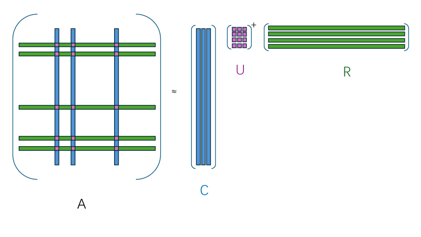
Figure 1: CUR Approximation

There has been extensive research on CUR Low-Rank Approximations for matrices. For readers interested in further details and additional references, please see the following works [1, 2, 4, 5, 9, 10, 11, 12, 13, 14, 15, 17, 19, 20, 21, 22, 23, 25, 26, 27, 28, 29, 30, 31, 32, 33, 34, 36, 40, 41, 46, 47, 48, 49, 50, 51, 52, 53] and the references cited therein. There are different strategies to obtain such CUR approximations or decomposition. This paper explore maximal volume optimization strategy within the framework of parallel computing.

I-B Maximal Volume Optimization

Definition 1

Given a square matrix $A\in\mathbb{R}^{r\times r},$ the volume of it is defined as absolute value of its determinant, i.e.,

$$\operatorname{vol}(A)=|det(A)|.$$

The CUR approximation with $r$ selected columns and rows is usually formulated as the following optimization problem [2, 15, 25, 26, 27, 37, 44, 53]

$$\operatorname*{argmax}_{\begin{subarray}{c}|\hat{I}|=|\hat{J}|=r\end{subarray}}\operatorname{vol}(A(\hat{I},\hat{J})).$$

The aforementioned optimization problem has numerous practical applications such as identifying the optimal nodes for polynomial interpolation over a given domain on appropriately discretized meshes [45] and preconditioning the iterative solution of linear least-squares problems [6].

Theorem 1 (cf. [26])

Let $A$ be a matrix of size $m\times n$ and $r$ be an integer satisfying $1\leq r<\min\{m,n\})$. Suppose that $I\subset\{1,\cdots,m\}$ with $\#(I)=r$ and $J\subset\{1,\cdots,n\}$ with $\#(J)=r$ such that $A_{I,J}$ has the maximal volume among all $r\times r$ submatrices of $A$. Then, the Chebyshev norm of the residual matrix satisfies the following estimate:

$$\|A-A_{r}\|_{C}\leq(r+1)\sigma_{r+1}(A),$$ (1)

where $A_{r}=A_{:,J}A_{I,J}^{\dagger}A_{I,:}$ is the $r$-cross approximation of $A$, $\sigma_{r+1}(A)$ is the $(r+1)^{th}$ singular value of $A$.

Recently, under the assumption in Theorem 1, Allen et.al [2] improve the error estimate bounds to the following the results.

Theorem 2 (cf. [2])

Under the assumption in Theorem 1, there is following estimate:

$$\|A-A_{r}\|_{C}\leq\frac{(r+1)\sigma_{r+1}(A)}{\sqrt{1+\sum\limits_{k=1}^{r}\frac{\sigma_{r+1}^{2}(A)}{\sigma_{k}^{2}(A)}}}$$

Theorem 1 and Theorem 2 tells us that the volume maximization can lead to a quasi-best low-rank approximation. However, identifying maximum-volume submatrices presents considerable computational challenges, as the problem is proven to be NP-hard [7]. This complexity has driven the development and adoption of greedy method-adaptive cross approximation-to provide practical solutions [8]. At its core, this method is highly connected to incomplete LU decomposition of the matrix [16]. We firstly introduce CUR Low-Rank Approximaation via Adaptive Cross Approximation Algorithm (ACA) [8] as follows.

Algorithm 1 Scalable Binary CUR Low-Rank Approximation Algorithm

1:Input: Matrix $A\in\mathbb{R}^{m\times n}$, target rank $r$.

2:Initialize $R_{0}:=A$, $I:=\{\},J:=\{\}.$

3:for $k=0,\ldots,m-1$ do

4:  $(i_{k+1},j_{k+1}):=\operatorname*{argmax}_{i,j}|R_{k}(i,j)|.$

5:  $I\leftarrow I\cup\{i_{k+1}\},J\leftarrow J\cup\{j_{k+1}\}.$

6:  $R_{k+1}:=R_{k}-\frac{1}{R_{k}(i_{k+1},j_{k+1})}R_{k}(:,j_{k+1})R_{k}(i_{k+1},:).$

7:end for

8:Output: $C=A(:,J),U=A(I,J),R=A(I,:).$

Each iteration in Algorithm 1 identifies a single pivot by searching for the largest absolute value in the residual matrix. Although local maxima searches can be conducted in parallel, a global reduction is necessary to determine the unique pivot element, thus creating an unavoidable sequential bottleneck. Once the pivot is found, the algorithm performs a rank-1 update on the residual, and this updated matrix in turn dictates the location and value of the next pivot. Consequently, there is a strict iteration-by-iteration data dependency, preventing the selection of multiple pivots simultaneously. In this paper, we propose the Scalable Binary CUR Low-Rank Approximation Algorithm. This framework is specifically designed to explore scalable CUR approximations for large-scale matrices by selecting rows and columns in parallel.

II Scalable Binary CUR Low-Rank Approximaation Algorithm

II-A Overview

The proposed Scalable Binary CUR Low-Rank Approximation Algorithm efficiently approximates a large-scale matrix $A\in\mathbb{R}^{n\times m}$ by decomposing it into three smaller matrices, $C$, $R$, and $U$. First, a binary parallel selection process, as detailed in Algorithm 3, identifies representative subsets of rows and columns from $A$. The matrix $C$ is constructed by extracting the columns of $A$ corresponding to the selected indices, while $R$ is formed by extracting the rows based on these indices. Finally, $U$ is computed as the pseudoinverse of the intersection submatrix $A(\text{rows},\text{cols})$. Together, these three matrices yield an efficient low-rank approximation of $A$.

Algorithm 2 Scalable Binary CUR Low-Rank Approximaation Algorithm

1:Input: Matrix $A\in\mathbb{R}^{n\times m}$, selected row count $r$, selected column count $c$

2:// Perform the following steps in parallel

3:Use Algorithm 3 to determine the set of row indices $I$.

4:Use Algorithm 3 to determine the set of column indices $J$.

5:Output: $C=A(:,J),U=A(I,J),R=A(I,:).$

Algorithm 3 Blockwise Adaptive Cross Approximation

1:Input: Matrix $A\in\mathbb{R}^{n\times m}$, number of selected indices $r$, number of blocks $b$, axis (0 for rows, 1 for columns)

2:Output: Selected indices $I$

3:$I=\{\}$ $\triangleright$ Initialize selected indices

4:if axis = 0 then

5:  Divide $A$ into $b$ blocks along rows: $A_{\text{block}}^{k}\in\mathbb{R}^{n_{k}\times m}$

6:  dimBlockSize $\leftarrow n_{k}$, dimSize $\leftarrow n$

7:else

8:  Divide $A$ into $b$ blocks along columns: $A_{\text{block}}^{k}\in\mathbb{R}^{n\times m_{k}}$

9:  dimBlockSize $\leftarrow m_{k}$, dimSize $\leftarrow m$

10:end if

11:for $i=0$ to $r-1$ do $\triangleright$ Select $r$ indices

12:  localMaxNorm, localMaxIdx $\leftarrow-1,-1$

13:  // Blockwise parallel selection of rows/columns with maximal norm

14:  for $i=0$ to $b\cdot\texttt{dimBlockSize}-1$ (parallel) do

15:   $k\leftarrow\lfloor i/\texttt{dimBlockSize}\rfloor$

16:   $j\leftarrow i\bmod\texttt{dimBlockSize}$

17:   $\texttt{globalIdx}\leftarrow i$

18:   if axis = 0 then

19:     $\texttt{localNorm}\leftarrow\operatorname{norm}(A_{\text{block}}^{k}(j,:))$

20:   else

21:     $\texttt{localNorm}\leftarrow\operatorname{norm}(A_{\text{block}}^{k}(:,j))$

22:   end if

23:   if localNorm $>$ localMaxNorm then

24:     localMaxNorm $\leftarrow$ localNorm

25:     localMaxIdx $\leftarrow$ globalIdx

26:   end if

27:  end for

28:  for $k=0$ to $b-1$ (parallel) do

29:   if localMaxNorm $>$ maxNorm then

30:     maxNorm $\leftarrow$ localMaxNorm

31:     maxIdx $\leftarrow$ localMaxIdx

32:   end if

33:  end for

34:  $k_{\text{block}}\leftarrow\texttt{maxIdx}\div\texttt{dimBlockSize}$

35:  $j_{\text{local}}\leftarrow\texttt{maxIdx}\bmod\texttt{dimBlockSize}$

36:  if axis = 0 then

37:   sharedMaxVec $\leftarrow A_{\text{block}}^{k}(j_{\text{local}},:)$

38:  else

39:   sharedMaxVec $\leftarrow A_{\text{block}}^{k}(:,j_{\text{local}})$

40:  end if

41:  // Parallel Blockwise update using shared max vector

42:  for $k=0$ to $b-1$ (parallel) do

43:   if axis = 0 then

44:     

$A_{\text{block}}^{k}\leftarrow A_{\text{block}}^{k}-\frac{A_{\text{block}}^{k}\cdot\texttt{sharedMaxVec}^{\top}}{\texttt{maxNorm}}\cdot\texttt{sharedMaxVec}$

45:   else

46:     

$A_{\text{block}}^{k}\leftarrow A_{\text{block}}^{k}-\texttt{sharedMaxVec}\cdot\left(\frac{\texttt{sharedMaxVec}^{\top}\cdot A_{\text{block}}^{k}}{\texttt{maxNorm}}\right)$

47:   end if

48:  end for

49:  $I(i)\leftarrow\texttt{maxIdx}$

50:end for

51:return $I$

II-B Blockwise Adaptive Cross Algorithm

The Blockwise Adaptive Cross Approximation algorithm is designed to efficiently select a subset of $r$ representative indices from a large matrix $A\in\mathbb{R}^{n\times m}$ by iteratively extracting the most significant row or column vectors. The algorithm begins by partitioning the matrix into $b$ blocks along a specified axis, determined by the parameter axis (where 0 indicates a row-wise partition and 1 indicates a column-wise partition). When axis is set to 0, $A$ is divided into blocks $A_{\text{block}}^{k}\in\mathbb{R}^{n_{k}\times m}$ along the rows; if axis is set to 1, the matrix is partitioned into blocks $A_{\text{block}}^{k}\in\mathbb{R}^{n\times m_{k}}$ along the columns. In this context, the variable dimBlockSize refers to the number of rows or columns in each block, while dimSize represents the total number of rows $n$ or columns $m$ in the matrix.

An empty global index set $I$ is then initialized to store the indices of the selected rows or columns. The algorithm proceeds over $r$ iterations, each intended to identify one key index. In each iteration, a parallel search is conducted within each block to compute the Euclidean norm of every candidate vector (row or column, depending on the specified axis). Each block determines its local maximum norm and the corresponding local index. These local maxima are subsequently combined through a reduction step that identifies the global maximum norm and its associated index, denoted as maxIdx.

Once the vector corresponding to maxIdx is identified, it is extracted from its block and referred to as sharedMaxVec. This vector is then employed to perform a rank-1 update on every block of the matrix. Specifically, if the operation is row-wise (i.e., axis = 0), the update involves subtracting from each block the product of the block and the transpose of sharedMaxVec divided by the squared norm of sharedMaxVec, multiplied by sharedMaxVec itself. Conversely, if the operation is column-wise (i.e., axis = 1), the subtraction is carried out by multiplying sharedMaxVec with the appropriate normalized factor computed from the block. This subtraction effectively removes the dominant component captured by the selected vector, ensuring that subsequent iterations focus on extracting new, non-redundant information.

The complete pseudo code is provided in Algorithm 3 for detailed reference.

The complexity of the Block Adaptive Cross Algorithm is determined by the operations performed in each iteration. Computing row norms for $n_{k}$ rows within a block requires $\mathcal{O}(n_{k}m)$ operations, and with $b$ blocks, this totals $\mathcal{O}\left(\frac{nm}{b}\right)$ per iteration. Updating the matrix, which includes projection, also requires $\mathcal{O}\left(\frac{nm}{b}\right)$ operations per iteration.

For $r$ iterations, the total complexity of the algorithm is: $\mathcal{O}\left(r\cdot\frac{nm}{b}\right).$ This represents a significant improvement over the sequential Adaptive Cross Approximation algorithm’s complexity of $O(r\cdot nm)$, particularly for large matrices and high levels of parallelism.

III Numerical Experiments

All experiments are conducted in a computing environment powered by an AMD EPYC 7H12 64-Core Processor running at 2.6 GHz. For matrix operations, we utilized Armiddol[42, 43], a high-performance matrix library designed to efficiently handle large-scale linear algebra computations.

III-A Approximation Error Study of Algorithm 2

In this section, we evaluate the performance of Algorithm 2 by testing its approximation capabilities on two types of data: Hilbert matrices and synthetic low-rank matrices. The key metric used for evaluation is the Frobenius norm relative error, defined as:

$$\text{Relative Error}=\frac{\|A-CUR\|_{F}}{\|A\|_{F}},$$

where $C$, $U$, and $R$ are the matrices resulting from the CUR Low-Rank Approximaation of $A$. This metric provides a quantitative assessment of the quality of the approximation and is consistently applied across all experiments.

Experiments on Hilbert Matrices

Hilbert matrices are well-known for their ill-conditioned nature and high sensitivity to numerical approximations [38]. The experiments assess the approximation error of Algorithm 2 applied to Hilbert matrices of varying dimensions ($256\times 256$, $512\times 512$, and $1024\times 1024$). For each matrix size, the number of selected rows and columns varied from $1$ to $20$. Figure 2 shows the relationship between the number of selected rows and columns and the approximation error.

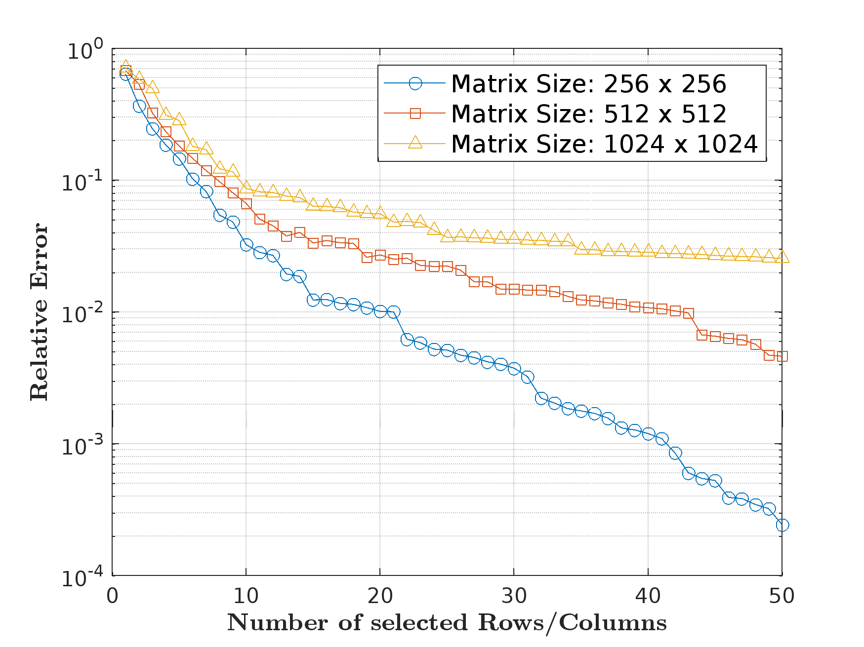
Figure 2: Approximation error of Algorithm 2 for Hilbert matrices. The x-axis represents the number of selected rows/columns, and the y-axis shows the Frobenius norm relative error.

The experimental results, illustrated in Figure 2, demonstrate the efficacy of Algorithm 2 in approximating matrices of varying sizes ($256\times 256$, $512\times 512$, and $1024\times 1024$) by examining the relationship between the number of selected rows/columns and the Frobenius norm relative error. Figure 2 reflects the algorithm’s ability to effectively capture the dominant features of the matrix.

Experiments on Synthetic Low-Rank Matrices

To further validate the algorithm, we conducted tests on synthetic low-rank matrices with controlled rank structures. These matrices were constructed by generating two matrices, $A$ and $B$, of sizes $n\times r$ and $r\times n$, respectively, with entries defined as:

$$A(i,j)=\frac{1}{i+j},\quad B(i,j)=\frac{1}{i+j},$$

where $i$ and $j$ denote the row and column indices. The synthetic low-rank matrix $H$ is generated by $H=A\cdot B.$ The experiments are performed on the generated matrix with sizes $n=256,512,1024$ and rank value $r=5,10,15,20$.

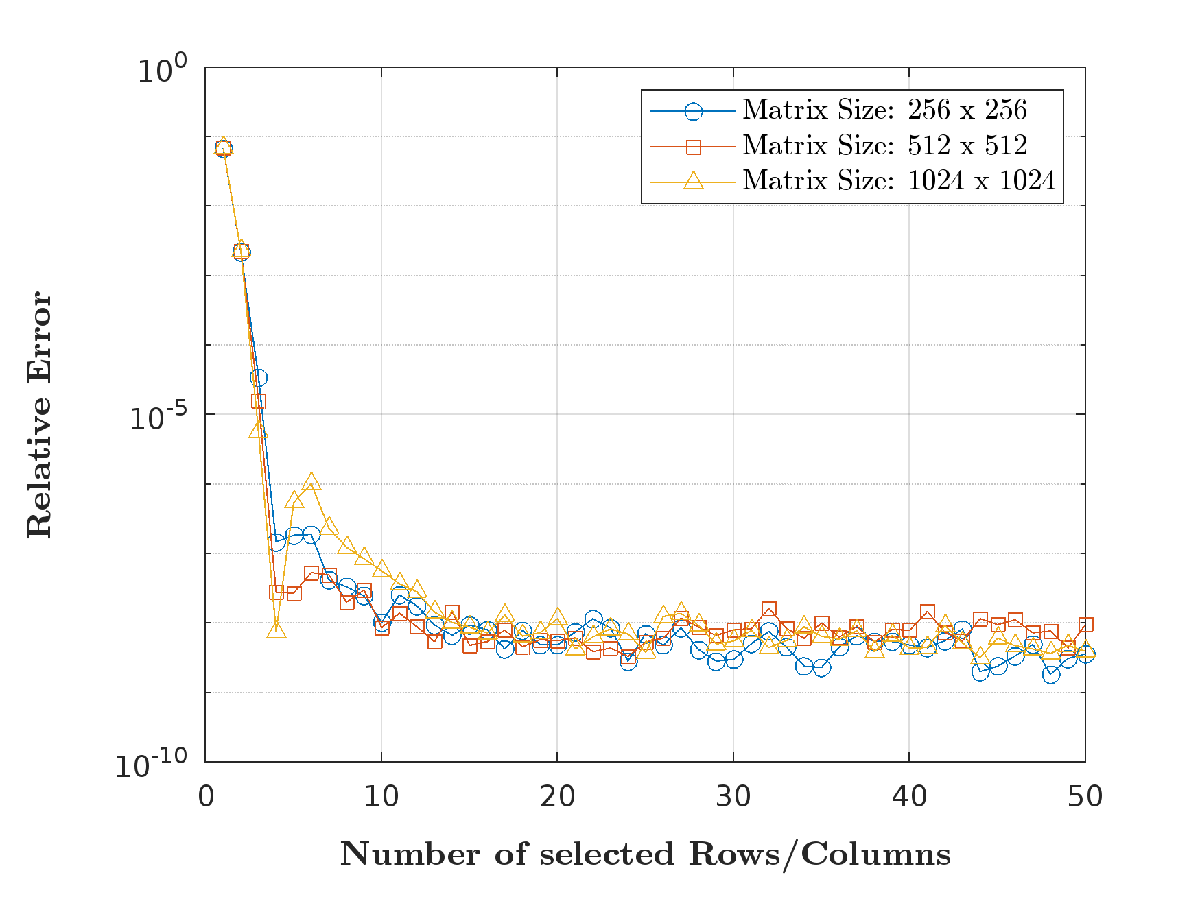
(a) Rank = 5

(b) Rank = 10

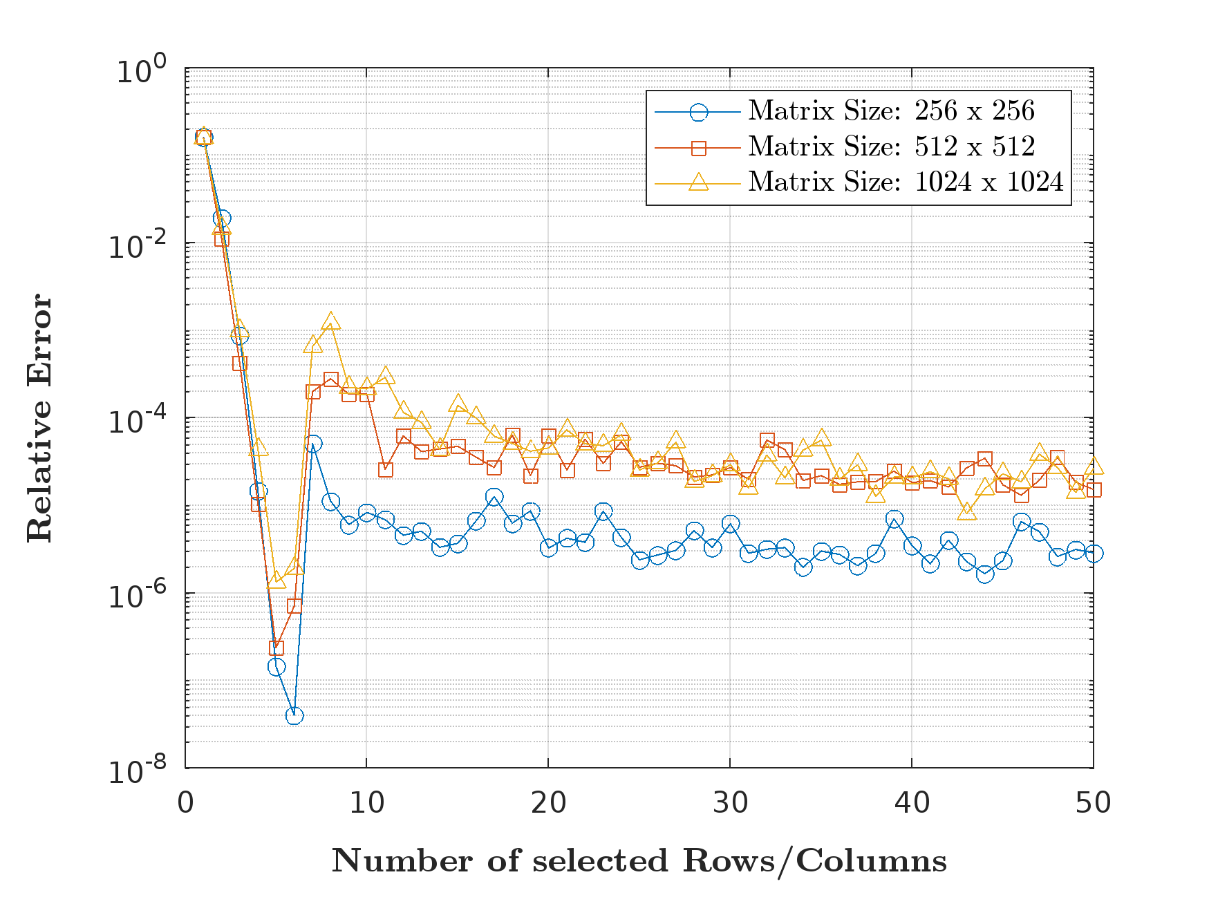
(c) Rank = 15

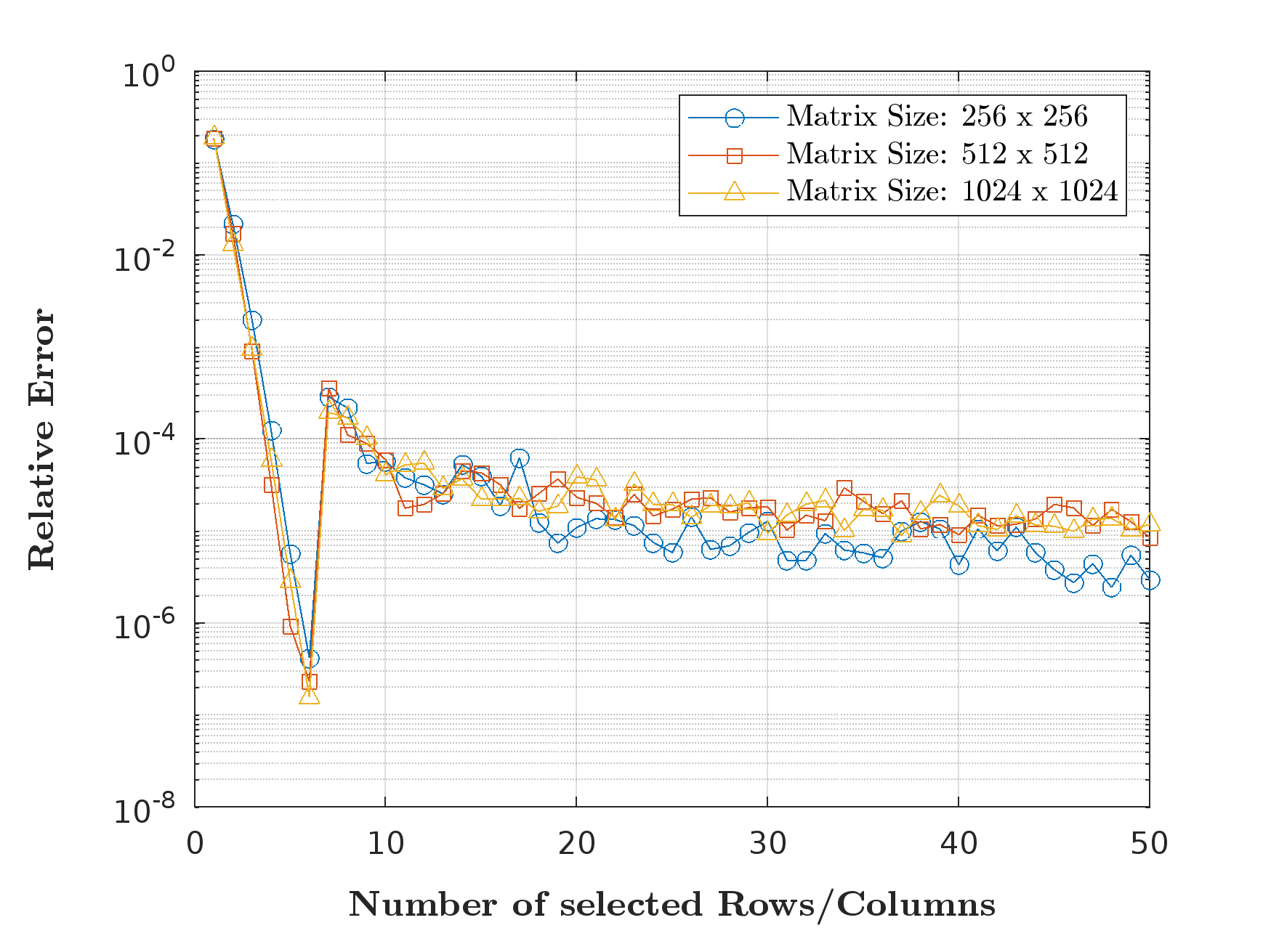
(d) Rank = 20

Figure 3: Relative Errors for Different Ranks

The results reveal that the Algorithm 2 achieves near-perfect approximation for low-rank matrices even with a small number of selected rows and columns. The relative error decreases sharply as $r$ increases and stabilizes at near-zero levels, reflecting the algorithm’s effectiveness in reconstructing matrices with well-defined rank structures.

III-B Scalability Analysis of Algorithm 2

In this section, we conduct a scalability analysis of Algorithm 2. The experiments focus on matrices of size $16384\times 16384$. We choose Algorithm 1 as sequential benchmark algorithm

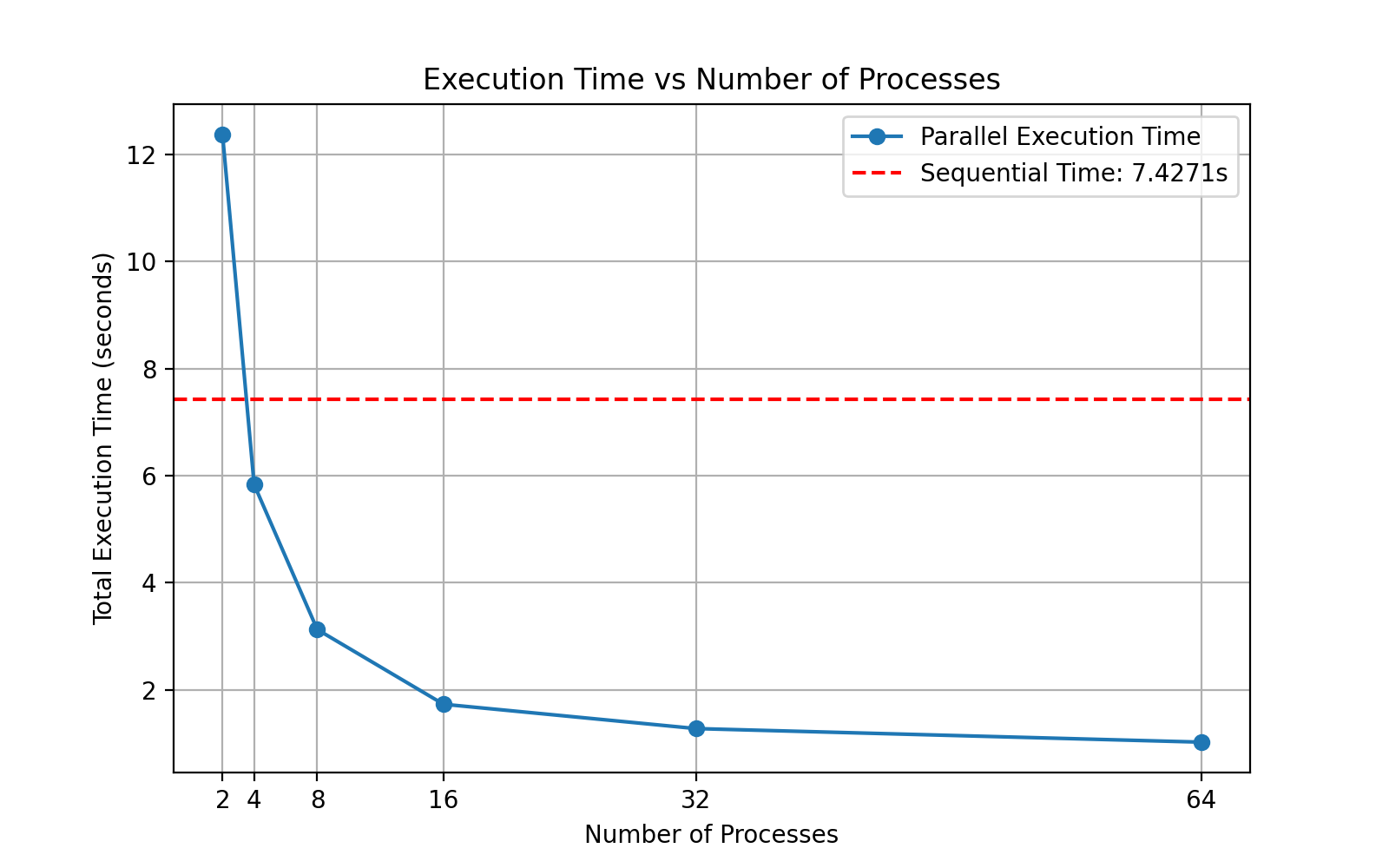
Figure 4: Caption

Figure 4 displays the relationship between the number of processes and the total execution time for the Algorithm 2. As the number of processes increases from 2 to 64, the execution time exhibits a decreasing trend, demonstrating the expected performance improvement with parallelization. Notably, the execution time reduces from 12.3733 seconds for two process to 1.02225 seconds when employing 64 processes. However, the performance gain is not strictly linear; the curve gradually flattens as the number of processes increases beyond 16, suggesting diminishing returns due to parallel overhead and potential communication costs. A red dashed line is plotted to indicate the sequential baseline time of 7.4271 seconds, which serves as a reference point. The data highlights that parallel execution with more than 4 processes consistently outperforms the sequential baseline. These results suggest that parallelization is effective in accelerating MaxVol computations, but the efficiency gain saturates at higher process counts, likely due to inter-process communication and synchronization overhead.

IV Conclusion

In conclusion, we have presented a Scalable Binary CUR Low-Rank Approximation Algorithm. This approach is designed to achieve CUR decomposition of large-scale matrices by deterministiclly selecting rows and columns in parallel. By leveraging the parallel processing capabilities of modern multi-core architectures, our approach has shown modest improvements in computational efficiency.

References

- [1] A. Aldroubi, K. Hamm, A. B. Koku, and A. Sekmen. CUR decompositions, similarity matrices, and subspace clustering. Frontiers in Applied Mathematics and Statistics, 4:65, 2019.
- [2] K. Allen, M.-J. Lai, and Z. Shen. Maximal volume matrix cross approximation for image compression and least squares solution. Advances in Computational Mathematics, 50(5):102, 2024.
- [3] O. Alter, P. O. Brown, and D. Botstein. Singular value decomposition for genome-wide expression data processing and modeling. Proceedings of the National Academy of Sciences, 97(18):10101–10106, 2000.
- [4] D. Anderson, S. Du, M. Mahoney, C. Melgaard, K. Wu, and M. Gu. Spectral gap error bounds for improving cur matrix decomposition and the nyström method. In Artificial intelligence and statistics, pages 19–27. PMLR, 2015.
- [5] D. Anderson and M. Gu. An efficient, sparsity-preserving, online algorithm for low-rank approximation. In International Conference on Machine Learning, pages 156–165. PMLR, 2017.
- [6] M. Arioli and I. S. Duff. Preconditioning linear least-squares problems by identifying a basis matrix. SIAM Journal on Scientific Computing, 37(5):S544–S561, 2015.
- [7] J. J. Bartholdi III. A good submatrix is hard to find. Operations Research Letters, 1(5):190–193, 1982.
- [8] M. Bebendorf. Approximation of boundary element matrices. Numerische Mathematik, 86:565–589, 2000.
- [9] C. Boutsidis and D. P. Woodruff. Optimal CUR matrix decompositions. In Proceedings of the forty-sixth annual ACM symposium on Theory of computing, pages 353–362, 2014.
- [10] H. Cai, K. Hamm, L. Huang, J. Li, and T. Wang. Rapid robust principal component analysis: Cur accelerated inexact low rank estimation. IEEE Signal Processing Letters, 28:116–120, 2021.
- [11] H. Cai, K. Hamm, L. Huang, and D. Needell. Robust cur decomposition: Theory and imaging applications. SIAM Journal on Imaging Sciences, 14(4):1472–1503, 2021.
- [12] Z. Cao, Y. Wei, and P. Xie. Randomized gcur decompositions. Advances in Computational Mathematics, 50(4):77, 2024.
- [13] S. Chaturantabut and D. C. Sorensen. Nonlinear model reduction via discrete empirical interpolation. SIAM Journal on Scientific Computing, 32(5):2737–2764, 2010.
- [14] C. Chen, M. Gu, Z. Zhang, W. Zhang, and Y. Yu. Efficient spectrum-revealing cur matrix decomposition. In International Conference on Artificial Intelligence and Statistics, pages 766–775. PMLR, 2020.
- [15] A. Civril and M. Magdon-Ismail. On selecting a maximum volume sub-matrix of a matrix and related problems. Theoretical Computer Science, 410(47-49):4801–4811, 2009.
- [16] A. Cortinovis, D. Kressner, and S. Massei. On maximum volume submatrices and cross approximation for symmetric semidefinite and diagonally dominant matrices. Lin. Alg. Appl., 593:251–268, 2020.
- [17] Y. Dong and P.-G. Martinsson. Simpler is better: A comparative study of randomized algorithms for computing the cur decomposition. arXiv preprint arXiv:2104.05877, 2021.
- [18] P. Drineas and M. W. Mahoney. CUR matrix decompositions for improved data analysis. Proceedings of the National Academy of Sciences, 106(3):697–702, 2008.
- [19] P. Drineas, M. W. Mahoney, and S. Muthukrishnan. Relative-error CUR matrix decompositions. SIAM Journal on Matrix Analysis and Applications, 30(2):844–881, 2008.
- [20] Z. Drmac and S. Gugercin. A new selection operator for the discrete empirical interpolation method—improved a priori error bound and extensions. SIAM Journal on Scientific Computing, 38(2):A631–A648, 2016.
- [21] M. Fornace and M. Lindsey. Column and row subset selection using nuclear scores: algorithms and theory for nystr”o m approximation, cur decomposition, and graph laplacian reduction. arXiv preprint arXiv:2407.01698, 2024.
- [22] I. Georgieva and C. Hofreither. On best uniform approximation by low-rank matrices. Linear Algebra and its Applications, 518:159–176, 2017.
- [23] P. Y. Gidisu and M. E. Hochstenbach. A restricted svd type cur decomposition for matrix triplets. SIAM Journal on Scientific Computing, 46(2):S401–S423, 2024.
- [24] G. Golub and W. Kahan. Calculating the singular values and pseudo-inverse of a matrix. Journal of the Society for Industrial and Applied Mathematics, Series B: Numerical Analysis, 2(2):205–224, 1965.
- [25] S. A. Goreinov, I. V. Oseledets, D. V. Savostyanov, E. E. Tyrtyshnikov, and N. L. Zamarashkin. How to find a good submatrix. In Matrix Methods: Theory, Algorithms And Applications: Dedicated to the Memory of Gene Golub, pages 247–256. World Scientific, 2010.
- [26] S. A. Goreinov and E. E. Tyrtyshnikov. The maximal-volume concept in approximation by low-rank matrices. Contemporary Mathematics, 280:47–52, 2001.
- [27] S. A. Goreinov and E. E. Tyrtyshnikov. Quasioptimality of skeleton approximation of a matrix in the chebyshev norm. In Doklady Mathematics, volume 83, pages 374–375. Springer, 2011.
- [28] S. A. Goreinov, E. E. Tyrtyshnikov, and N. L. Zamarashkin. A theory of pseudoskeleton approximations. Linear algebra and its applications, 261(1-3):1–21, 1997.
- [29] M. Gu and S. C. Eisenstat. Efficient algorithms for computing a strong rank-revealing QR factorization. SIAM Journal on Scientific Computing, 17(4):848–869, 1996.
- [30] K. Hamm and L. Huang. Cur decompositions, approximations, and perturbations. arXiv preprint arXiv:1903.09698, 2019.
- [31] K. Hamm and L. Huang. Perspectives on cur decompositions. Applied and Computational Harmonic Analysis, 48(3):1088–1099, 2020.
- [32] K. Hamm and L. Huang. Stability of sampling for cur decompositions. Foundations of Data Science, 2(2):83–99, 2020.
- [33] K. Hamm and L. Huang. Perturbations of cur decompositions. SIAM Journal on Matrix Analysis and Applications, 42(1):351–375, 2021.
- [34] Y. Ida, S. Kanai, Y. Fujiwara, T. Iwata, K. Takeuchi, and H. Kashima. Fast deterministic cur matrix decomposition with accuracy assurance. In International Conference on Machine Learning, pages 4594–4603. PMLR, 2020.
- [35] D. Liben-Nowell and J. Kleinberg. The link prediction problem for social networks. In Proceedings of the twelfth international conference on Information and knowledge management, pages 556–559, 2003.
- [36] M. W. Mahoney and P. Drineas. CUR matrix decompositions for improved data analysis. Proceedings of the National Academy of Sciences, 106(3):697–702, 2009.
- [37] A. Mikhalev and I. V. Oseledets. Rectangular maximum-volume submatrices and their applications. Linear Algebra and its Applications, 538:187–211, 2018.
- [38] M. Morháč. An algorithm to solve hilbert systems of linear equations precisely. Applied mathematics and computation, 73(2-3):209–229, 1995.
- [39] C.-T. Pan. On the existence and computation of rank-revealing LU factorizations. Linear Algebra and its Applications, 316(1-3):199–222, 2000.
- [40] T. Park and Y. Nakatsukasa. Accuracy and stability of cur decompositions with oversampling. arXiv preprint arXiv:2405.06375, 2024.
- [41] T. Park and Y. Nakatsukasa. Low-rank approximation of parameter-dependent matrices via cur decomposition. arXiv preprint arXiv:2408.05595, 2024.
- [42] C. Sanderson and R. Curtin. Armadillo: a template-based C++ library for linear algebra. Journal of Open Source Software, 1(2):26, 2016.
- [43] C. Sanderson and R. Curtin. Practical sparse matrices in C++ with hybrid storage and template-based expression optimisation. Mathematical and Computational Applications, 24(3):70, 2019.
- [44] J. Schneider. Error estimates for two-dimensional cross approximation. Journal of approximation theory, 162(9):1685–1700, 2010.
- [45] A. Sommariva and M. Vianello. Computing approximate fekete points by QR factorizations of vandermonde matrices. Computers & Mathematics with Applications, 57(8):1324–1336, 2009.
- [46] D. C. Sorensen and M. Embree. A DEIM induced CUR factorization. SIAM Journal on Scientific Computing, 38(3):A1454–A1482, 2016.
- [47] C. Thurau, K. Kersting, and C. Bauckhage. Deterministic cur for improved large-scale data analysis: An empirical study. In Proceedings of the 2012 SIAM International Conference on Data Mining, pages 684–695. SIAM, 2012.
- [48] S. Voronin and P.-G. Martinsson. Efficient algorithms for cur and interpolative matrix decompositions. Advances in Computational Mathematics, 43:495–516, 2017.
- [49] S. Wang and Z. Zhang. A scalable CUR matrix decomposition algorithm: Lower time complexity and tighter bound. Advances in Neural Information Processing Systems, 25, 2012.
- [50] S. Wang and Z. Zhang. Improving CUR matrix decomposition and the Nyström approximation via adaptive sampling. The Journal of Machine Learning Research, 14(1):2729–2769, 2013.
- [51] S. Wang, Z. Zhang, and T. Zhang. Towards more efficient spsd matrix approximation and CUR matrix decomposition. Journal of Machine Learning Research, 17(209):1–49, 2016.
- [52] J. Xia. Making the nyström method highly accurate for low-rank approximations. SIAM Journal on Scientific Computing, 46(2):A1076–A1101, 2024.
- [53] N. Zamarashkin and A. Osinsky. New accuracy estimates for pseudoskeleton approximations of matrices. In Doklady Mathematics, volume 94, pages 643–645. Springer, 2016.