Global attractivity criteria for a discrete-time Hopfield neural network model with unbounded delays via singular matrices
José J. Oliveira∗, Ana Sofia Teixeira‡
() Centro de Matemática (CMAT), Departamento de Matemática,
Universidade do Minho, Campus de Gualtar, 4710-057 Braga, Portugal
e-mail: jjoliveira@math.uminho.pt
() Departamento de Matemática, Universidade do Minho, Campus de Gualtar, 4710-057 Braga, Portugal
e-mail: pg49167@alunos.uminho.pt
Abstract
In this work, we establish two global attractivity criteria for a multidimensional discrete-time non-autonomous Hopfield neural network model with infinite delays and delays in the leakage terms. The first criterion, which applies when the activation functions are bounded, is based on matrices that are not necessarily invertible. The second criterion, relevant for unbounded activation functions, requires that a related singular matrix be irreducible. We contrast our findings with existing results in the literature and present numerical simulations to illustrate the efficacy of the proposed criteria.
Keywords: Hopfield neural network model, global attractivity, difference equation, infinite time delay, matrix, irreducible matrix
Mathematics Subject Classification System 2020: 39A10, 39A30, 39A60, 92B20.
1 Introduction
Neural network models have emerged as indispensable tools across diverse scientific and engineering domains, offering innovative solutions to complex challenges. Their applications span optimization [7], signal processing [7], image processing [1], and pattern classification [24], where they effectively learn intricate patterns and relationships within data, resulting in highly accurate solutions. Essential attributes such as associative memory, parallel computation, pattern categorization, and fault tolerance [14] underscore their wide-ranging utility.
In his pioneering work, the recent Nobel Prize winner in Physics, John Hopfield proposed a system of ordinary differential equations to describe an artificial neural network [15]. To better represent the inherent delays in neural signal transmission, such as finite signal propagation speeds and neuron response times, delays were incorporated into Hopfield’s model. Marcus and Westervelt [18] demonstrated how such delays can destabilize the system. Since then, numerous studies on the stability of neural network models with delays have been published (see, for example, [2, 4, 8, 11, 21] and references therein).
Although the stability analysis of continuous-time neural networks has received substantial attention, the discrete-time counterparts are equally important due to their relevance in computational implementations. As noted in [19], discrete-time systems may not fully replicate the dynamics of their continuous-time analogs, thus it is worthwhile to study the stability of discrete-time neural network models with delays. This paper focuses on providing sufficient conditions for the global attractivity of a general discrete-time non-autonomous Hopfield neural network model incorporating infinite distributed delays and time-varying delays in the leakage terms. Unlike many existing stability criteria based on -matrices that require these matrices to be non-singular, our results allow for singular -matrices, thereby broadening their applicability. As far as we are aware, the exceptions are the work of Hong and Ma [13] for an autonomous discrete-time Hopfield type model with finite delays and the work of Ma, Saito, and Takeuchi [17] for an autonomous continuous-time Hopfield type model also with finite delays.
In [20], the author established sufficient conditions, involving non-singular matrices, for the existence and global asymptotic stability of an equilibrium in an autonomous continuous-time Hopfield neural network model with infinite distributed delays. Recently, in [10], the main result from [20] was generalized to a continuous-time Cohen-Grossberg neural network model, also involving non-singular matrices. For continuous-time Bidirectional Associative Memory(BAM) neural network models with delays in the leakage terms, [4] established sufficient conditions for global asymptotic stability, again involving non-singular matrices. Subsequently, in [22], the main result from [4] was improved, still assuming that a certain matrix is a non-singular matrix.
The stability of discrete-time neural network models has been less studied compared to continuous-time models, and stability results for discrete-time neural network models with infinite delays remain relatively scarce [6, 21]. The use of models with infinite delays allows the modeling of phenomena where the present evolution depends on the entire past history. It is worth noting that difference equations with finite delays can be transformed into delay-free difference equations by increasing the dimension of the realization space [9], which could potentially make their study easier.
In [3, 8, 21, 16], sufficient conditions for the global exponential stability of various discrete-time Hopfield neural network models involving non-singular matrices were established. Specifically, [3] provided sufficient conditions for the existence and global exponential stability of a periodic solution to a general difference equation with finite delays. This stability criterion was applied to both low-order and high-order periodic Hopfield neural network models, as well as to a BAM neural network model, with a finite delay in the leakage terms, yielding stability criteria involving non-singular matrices. In [8], respectively in [16], a criterion for the exponential stability of a discrete-time high-order, respectively low-order, Hopfield-type neural network model with finite delays and impulses was established, again involving non-singular matrices. In [21] a global exponential stability criterion was established for a general difference equation with infinite delays and applied to discrete-time Hopfield models with both infinite delays and finite delays in the leakage terms.
There are several studies on the stability of neural network models with delays on time-scales, but those that establish stability criteria involving matrices do so under the assumption that they are non-singular (see, for example, [12]).
The main contributions of this paper are:
- i.
-
The new technique developed to establish the global stability criteria of the model employing the properties of M-matrices and irreducible singular M-matrices, without requiring their invertibility or the construction of Lyapunov functionals, as is often observed in the literature;
- ii.
-
The global attractivity criterion, involving matrices non-necessarily invertible, established for the discrete-time non-autonomous Hopfield neural network model with infinite distributed and time-varying delays, system (2), assuming bounded activation functions that are not required to be differentiable or monotonic, item i. of Theorem 3.4. It is worth noting that in [13], the global attractivity criterion was obtained for the autonomous model with finite delays, system (25), assuming bounded, monotonic, and differentiable activation functions;
- iii.
-
The stability criterion, involving singular irreducible matrices, for the same model (2) without the assumption that the activation functions are bounded, item ii. of Theorem 3.4. We stress the importance of studying neural network models with unbounded activation functions [23], such as Gaussian Error Linear Unit (GELU) functions. To the best of our knowledge, existing stability criteria for neural network models with unbounded activation functions, when involving -matrices, typically assume that these matrices are non-singular (see [8, 21] and references therein).
After this introduction, Section 2 outlines the key notations, provides fundamental results from the theory of matrices, and introduces the discrete-time non-autonomous Hopfield neural network model considered in this work, which includes infinite distributed delays and time-varying delays in the leakage terms. Section 3 constitutes the main contribution of the paper, where we establish the global attractiveness results. A comparison of our results with those available in the literature is also provided. In Section 4, we include two numerical examples to illustrate the obtained results and highlight their originality in comparison with previous findings. The paper concludes with a brief discussion and summary of the main contributions.
2 Preliminaries and Model Description
For , we denote by the set of integers numbers . In this paper, for , we always consider the Banach space with the norm
Given , we write if for all , and if for all . We write , for any . For a real number , we denote its integer part by .
For , we denote the set of real matrices by and, as usual, we define
Given , we write if for all . We denote by the transpose of matrix .
Definition 2.1.
Let and .
We say that is an matrix if all principal minors are non-negative.
We say that is a non-singular matrix if all principal minors are positive.
A large number of equivalent properties exist for identifying matrices and non-singular matrices. For a detailed discussion of some of these properties, we refer the reader to Chapter 6 of [5]. In this paper, we need the following result:
Theorem 2.1.
[5, Theorem 4.4.6] Let .
The matrix is an matrix if and only if, for any and taking , there is such that and .
Definition 2.2.
[5, Definition 2.1.2] A square matrix is reducible if there is a permutation matrix such that
where are square matrices, or if and . Otherwise is called irreducible.
We also need the following result:
Theorem 2.2.
[5, Theorem 6.4.16] If is a singular irreducible matrix of order , then there is such that .
For a continuous function such that , we denote by the function defined by
| (1) |
where the functions and are defined by
respectively. It is straightforward to verify that is a non-decreasing continuous function such that for all .
For , we denote by the space of bounded functions , with the norm
For and a vector function such that , we define by
In this paper, we investigate the following generalized discrete-time non-autonomous Hopfield neural network model that incorporates both infinite distributed delays and time-varying delays, with the latter also present in the leakage terms:
| (2) | |||||
where , , , , , and are functions. This discrete-time model generalizes several existing models in the literature, including those investigated in [13, 19, 21].
3 Global attractiveness
In this section, we give two global attractivity criteria for model (2). For this purpose, we consider the following set of hypotheses: For each and ,
- (H1)
-
we have
- (H2)
-
we have
- (H3)
-
the functions and are bounded;
- (H4)
-
we have
- (H5)
-
we have
Depending on whether the activation functions and are bounded, one of the following hypothesis is also assumed.
- (H6)
-
the functions are continuous and there exist constants such that
or
- (H6*)
-
the functions are continuous and there exist constants such that
Remark 3.1.
Note that, from (H6) or (H6*) we have for all and .
From (H3), we denote
| (4) |
and
| (5) |
Now, consider the matrices defined by
| (6) |
where , and
| (7) |
where , respectively. Note that we have .
In order to obtain the stability criteria, we first need to prove that all solutions of (2) are bounded.
Lemma 3.2.
Proof.
Proof of item i.
For and , consider the solution of (2)-(3). From (2), (4), and hypothesis (H6) we obtain
and by the hypotheses (H4) and (H5), we have
that is
| (8) |
where and .
We claim that
| (9) |
and, since , we conclude that the solution is bounded.
In fact, for , inequality (8) implies
and
Assuming that (9) holds for some , from (8) we have
and by the induction hypothesis we obtain
and the proof of item i is done.
Proof of item ii.
Since is a singular irreducible matrix, Theorem 2.2 implies the existence of such that , that is
| (10) |
With the change , for all , model (2) assumes the form
| (11) | |||||
For and , consider the solution of (2)-(3). Suppose, by contradiction, that the solution is unbounded. Consequently is also an unbounded solution of (11) and there exist and such that
| (12) |
where . If not, then we have
thus
where and . Consequently
and, from (H5), we conclude that is bounded which is a contradiction. Thus (12) holds.
Lemma 3.3.
Proof.
Proof of item i.
For and , consider the solution of (2)-(3). Item i. of Lemma 3.2 assures that is bounded, thus for all .
From (2) and hypotheses (H4) and (H6) we have
and from (H5) and (5) we obtain
The solution is bounded, by hypothesis (H2), and , then
| (16) |
Consequently, given there is such that
| (17) |
Form (H2), for each and , there is such that for . Defining we have
| (18) |
From (H4), there is such that
| (19) |
Defining , for and we have thus, from (17) we obtain
| (20) |
Recalling the definition of for a given function in (1), we know that, for each and , and are non-decreasing continuous functions such that
More, from (H6) it is easy to conclude that and satisfy (H6) with the same constants and , respectively.
From model (2) and the properties of and described above, for all and we have
The functions and are non-decreasing satisfying (H6) thus, from (H4), (18), (19), and (20), for we have
| (21) | |||||
Consequently, from (H5) and (5),
As and are continuous and is arbitrary, we conclude that
As , , and (16), then for all . Iterating the previous process, for each , we obtain a non-increasing sequence such that , , and
| (22) |
Defining , we have
Finally, from (22) and the continuity of and we conclude that
Proof of item ii.
For and , consider the solution of (2)-(3). Item ii. of Lemma 3.2 assures that is bounded, thus we may define
For each also define .
Given there is such that
Arguing as in the previous item, we conclude an estimation analogous to (21), i.e. there is such that, for all and ,
Consequently,
and applying again the in both sides and taking , we obtain
As and satisfy (H6*), then and also satisfy (H6*), and consequently for all .
Finally, by repeating the arguments presented in the proof of the previous item i., we conclude the existence of such that , for all , and (15) holds. ∎
Now we are in position to prove the main result of this paper.
Theorem 3.4.
Proof.
Here we present only the proof of item i.. The proof of item ii. follows similarly putting the matrix instead of . Recall the definitions of the matrices and in (6) and (7), respectively.
To conclude the proof it is enough to prove that for all .
First, we assume that . As and also satisfy (H6), then and for all and . Consequently, from (14), we obtain
for all , thus with . Considering and , we have
which is not possible because of being an matrix (see Theorem 2.1).
Now, suppose that there is such that and for all . We do not lose generality if we assume that . Thus we have and for . Consequently, from (14) we obtain
and by the same argument as before we get another contradiction thus there is such that .
After steps we conclude that . From (14) we have
If , then
thus
which is not possible because of Theorem 2.1 again. Consequently and the proof is concluded. ∎
Let us now take the following autonomous discrete-time Hopfield model with infinite delays
| (23) | |||||
where and, for each and , , , , and are functions.
As an immediate consequence of Theorem 3.4, we derive the following global stability criteria for the autonomous discrete-time Hopfield neural network model (23).
Corollary 3.5.
Assume that for all and that hypothesis (H4) holds.
Defining , consider the matrix
| (24) |
- 1.
- 2.
By taking , , , , and in (23) for all , we obtain the next discrete-time Hopfield model with finite delays:
| (25) |
and the matrix defined in (24) takes the form
where . We note that model (25) has finite delays. Consequently, it is possible to transform it into a non-delay discrete-time model, making it easier to handle than (23).
Remark 3.6.
In [13, Theorem 3.1], the global attractivity of (25) is established under the assumption that is an matrix and the activation functions, , are differentiable, satisfying the conditions
and
| (26) |
These conditions are more restrictive than hypothesis (H6). Additionally model (23) includes both infinite delays and delays in the leakage terms. Together, theses factors demonstrate that item i. in Corollary 3.5 provides a significant improvement over the global criterion presented in [13]. We note that the authors in [13] wrote the hypothesis instead of (26). However, this is inaccurate because (26) is need to obtain in [13, page 4940, line 5].
Now, taking , , , and in (23) for all , we obtain the following model
| (27) | |||||
and the matrix defined in (24) has the form
where .
Assume that for all , and that hypotheses (H4) and (H6*) hold. From Corollary 3.5, we conclude that if is a singular irreducible matrix, then the zero solution of (27) is globally attractive within the set of solutions with bounded initial conditions.
Remark 3.7.
Now, we present a global attractivity criterion for the case where the activation functions in (23) are Lipschitz functions.
Corollary 3.8.
Assume that (23) has an equilibrium point , and that hypotheses (H4) and
- (H6†)
-
For each and , there exist constants such that
for with ,
hold.
4 Numerical Examples
Here, we provide two numerical examples to highlight the effectiveness of the new results given in this work.
Example 4.1. In model (2) we take , , the following coefficients in the leakage terms
the delays in the leakage terms
the coefficients in the terms with discrete time-varying delays
the coefficients in the terms with distributed delays
and the discrete time-varying delays
recalling that denotes the integer part of the real number . We also take the activation functions
the Kernel factors in the terms with infinite distributed delays
for , and the external inputs
In this example we have , for and , and the matrix in (7) has the form
which is a singular M-matrix. As the hypothesis (H1)-(H6) hold, item i. of Theorem 3.4 ensures that all solutions, with and , of this example converge to as tends to infinity. Figure 1 shows the plot of the solution of this illustrative numerical example with initial condition .
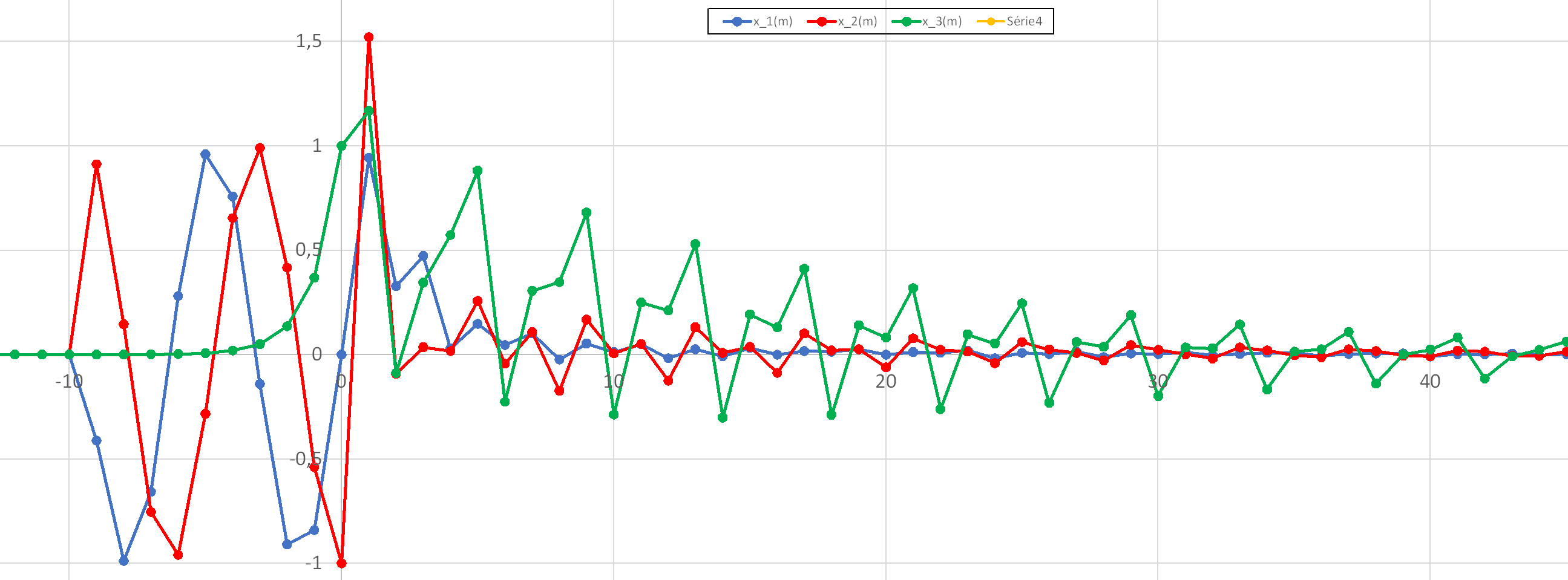
We note that this numerical example is non-autonomous and has unbounded delays. Therefore, the stability criterion established in [13] cannot be applied in this case.
Example 4.2. In this second numerical example consider, in model (2), , , the coefficients in the leakage terms
the delays in the leakage terms
the coefficients in the terms with discrete time-varying delays
the coefficients in the terms with distributed delays
the discrete time-varying delays
the activation functions
the Kernel factors in the terms with infinite distributed delays
for , and the external inputs
We have for and , and the matrix in (6) has the form
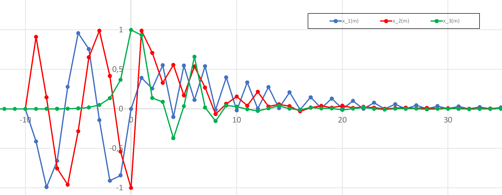
which is a singular irreducible matrix. As the hypotheses (H1)-(H5) and (H6*) hold, item ii. of Theorem 3.4 ensures that all solutions, with and , of this example converge to as tends to infinity. Figure 2 shows the plot of the solution of this illustrative numerical example with initial condition .
We note that in this numerical example, there are unbounded delays and some activation functions are also unbounded. Therefore, the stability criterion established in [13] also cannot be applied in this case.
5 Conclusions
In this work, we have established two global attractivity criteria for a discrete-time non-autonomous Hopfield neural network model with infinite distributed and time-varying delays (Theorem 3.4). Notably, unlike the common assumptions in the literature, the stability criteria presented here involve -matrices that are not necessarily invertible.
The first main stability criterion, outlined in item i. of Theorem 3.4, assumes that the activation functions of the model are bounded and sublinear. The second main stability criterion, presented in item ii. of Theorem 3.4, requires only that the activation functions be sublinear, with the additional assumption that the -matrix is singular and irreducible.
The two numerical simulations provided illustrate the practical implications and insights offered by this work.
Acknowledgments.
The research was partially financed by Portuguese Funds through FCT (Fundação para a Ciência e a Tecnologia) within the Projects UIDB/00013/2020 and UIDP/00013/2020 of CMAT-UM.
References
- [1] Aizenberg, I., Aizenberg, N., Hiltner, J., Moraga, C. and Zu Bexten, E. M., Cellular neural networks and computational intelligence in medical image processing, Image Vis. Comput., 19(4) (2001), 177–183.
- [2] Aktas, E., Faydasicok, O. and Arik, S., Robust stability of dynamical neural networks with multiple time delays: a review and new results, Artif. Intell. Rev., 56 (Suppl 2) (2023), 1647–1684.
- [3] Bento, A. J., Oliveira, J. J. and Silva, C. M., Existence and stability of a periodic solution of a general difference equation with applications to neural networks with a delay in the leakage terms, Commun Nonlinear Sci Numer Simul, 126 (2023), 107429.
- [4] Berezansky, L., Braverman, E. and Idels, L., New global exponential stability criteria for nonlinear delay differential systems with applications to BAM neural networks, Appl. Math. Comput., 243 (2014), 899–910.
- [5] Berman, A. and Plemmons, R. J., Nonnegative matrices in the mathematical sciences, Society for Industrial and Applied Mathematics, 1994.
- [6] Chen, X., Song, Q., Zhao, Z. and Liu, Y. Global stability analysis of discrete-time complex-valued neural networks with leakage delay and mixed delays, Neurocomputing, 175 (2016), 723–735.
- [7] Cochocki, A. and Unbehauen, R., Neural networks for optimization and signal processing, John Wiley & Sons, Inc., 1993.
- [8] Dong, Z., Zhang, X. and Wang, X., Global exponential stability of discrete-time higher-order Cohen-Grossberg neural networks with time-varying delays, connection weights and impulses, J. Franklin Inst., 358(11) (2021), 5931–5950.
- [9] Elaydi, S., An Introduction to Difference Equations, Springer Science + Business Media, Inc., 2005.
- [10] Elmwafy, A., Oliveira, J. J. and silva, C. M., Existence and exponential stability of a periodic solution of an infinite delay differential system with applications to Cohen-Grossberg neural networks, Commun Nonlinear Sci Numer Simul, 135 (2024), 108053.
- [11] Faria, T. and Oliveira, J. J., General criteria for asymptotic and exponential stabilities of neural network models with unbounded delays, Appl. Math. Comput., 217(23) (2011), 9646–9658.
- [12] Gao, J., Wang, Q. R. and Lin, Y., Existence and exponential stability of almost-periodic solutions for MAM neural network with distributed delays on time scales, Appl. Math., 36(1) (2021), 70–82.
- [13] Hong, Y. and Ma, W. Sufficient and necessary conditions for global attractivity and stability of a class of discrete Hopfield-type neural networks with time delays, Math. Biosci. Eng., 16(5) (2019), 4936–4946.
- [14] Hopfield, J. J., Neural networks and physical systems with emergent collective computational abilities Proc. Natl. Acad. Sci. U.S.A., 79(8) (1982), 2554–2558.
- [15] Hopfield, J. J., Neurons with graded response have collective computational properties like those of two-state neurons, Proc. Natl. Acad. Sci. U.S.A., 81(10) (1984), 3088–3092.
- [16] Li, W., Zhang, X., Liu, C. and Yang, X. Global Exponential Stability Conditions for Discrete-Time BAM Neural Networks Affected by Impulses and Time-Varying Delays, Circuits, Syst. Signal Process. (2024), 1-19.
- [17] Ma, W., Saito, Y. and Takeuchi, Y., matrix structure and harmless delays in a Hopfield-type neural network, Appl. Math. Lett., 22(7) (2009), 1066–1070.
- [18] Marcus, C. M. and Westervelt, R. M., Stability of analog neural networks with delay, Phys. Rev. A, 39(1) (1989), 347.
- [19] Mohamad, S. and Gopalsamy, K., Exponential stability of continuous-time and discrete-time cellular neural networks with delays, Appl. Math. Comput., 135(1) (2003), 17–38.
- [20] Ncube, I., Existence, uniqueness, and global asymptotic stability of an equilibrium in a multiple unbounded distributed delay network, Electron. J. Qual. Theory Differ. Equ., (59) (2020), 1–11.
- [21] Oliveira, J. J., Global exponential stability of discrete-time Hopfield neural network models with unbounded delays, J. Differ. Equ. Appl., 28(5) (2022), 725–751.
- [22] Oliveira, J. J., Global stability criteria for nonlinear differential systems with infinite delay and applications to BAM neural networks, Chaos Solitons Fractals, 164 (2022), 112676.
- [23] Sonoda, S. and Murata, N., Neural network with unbounded activation functions is universal approximator Appl. Comput. Harmon. Anal., 43 (2017), 233–268.
- [24] Zhang, D. and Lou, S., The application research of neural network and BP algorithm in stock price pattern classification and prediction, Future Gener. Comput. Syst., 115 (2021), 872–879.