Using Subspace Algorithms for the Estimation of Linear State Space Models for Over-Differenced Processes

Abstract

Subspace methods like canonical variate analysis (CVA) are regression based methods for the estimation of linear dynamic state space models. They have been shown to deliver accurate (consistent and asymptotically equivalent to quasi maximum likelihood estimation using the Gaussian likelihood) estimators for invertible stationary autoregressive moving average (ARMA) processes.
These results use the assumption that the spectral density of the stationary process does not have zeros on the unit circle. This assumption is violated, for example, for over-differenced series that may arise in the setting of co-integrated processes made stationary by differencing. A second source of spectral zeros is inappropriate seasonal differencing to obtain seasonally adjusted data. This occurs, for example, by investigating yearly differences of processes that do not contain unit roots at all seasonal frequencies.
In this paper we show consistency for the CVA estimators for vector processes containing spectral zeros. The derived rates of convergence demonstrate that over-differencing can severely harm the asymptotic properties of the estimators making a case for working with unadjusted data.

organization=Bielefeld University,addressline=Universitätsstrasse 25, city=Bielefeld, postcode=33615, state=NRW, country=Germany

1 Introduction

Subspace algorithms such as the Canonical Variate Analysis (CVA) (Larimore, 1983) are used for the estimation of linear dynamical state space systems for time series. CVA is popular since it is numerically cheap (consisting of a series of regressions), asymptotically equivalent to quasi maximum likelihood estimation (using the Gaussian likelihood) for stationary processes and robust to the existence of simple unit roots (see Bauer, 2005, for a survey). This robustness also carries over to the case of seasonal unit roots, see Bauer and Buschmeier (2021).

The algorithm fits a state space system in innovation form

$$y_{t}=Cx_{t}+\varepsilon_{t},\quad x_{t+1}=Ax_{t}+B\varepsilon_{t},\quad t\in{\mathbb{Z}},$$ (1)

to an observed multivariate time series $y_{t}\in{\mathbb{R}}^{s},t=1,...,T$. Here $A\in{\mathbb{R}}^{n\times n},B\in{\mathbb{R}}^{n\times s},C\in{\mathbb{R}}^{s\times n}$ define the state space system with system order $n$, which must be supplied to the algorithm. In this paper we will always assume that the system is minimal (implying that the state dimension cannot be reduced, see Hannan and Deistler, 1988, Chapter 1, for details) and stable (such that all eigenvalues of $A$ are smaller than one in modulus).

The innovation form representation given above corresponds to the Wold representation of the stationary process $(y_{t})_{t\in{\mathbb{Z}}}$, if and only if the eigenvalues of the matrix $\underline{A}=A-BC$ are inside or on the unit circle: In this case $\lambda_{|max|}(\underline{A})\leq 1$ where $\lambda_{|max|}(M)$ denotes a maximum modulus eigenvalue of the matrix $M$.

The asymptotic properties for CVA, when the data are generated from a stable state-space system, are documented in the literature; see, for example, Bauer (2005). However, results are restricted to the case of processes, where the strict inequality $\lambda_{|max|}(\underline{A})<1$ holds.

This restriction may be violated, in particular, for economic data, if the data are transformed to stationarity by temporal differencing of all components. If co-integrating relations between the component variables exist and the whole time series is differenced, this leads to over-differencing in some directions introducing spectral zeros at frequency $\omega=0$. Similar effects occur due to yearly differencing of time series, if not all unit roots to all seasonal frequencies are present. This happens, for example, if for an $I(1)$ process observed at quarterly frequency, yearly differences are examined. The corresponding seasonally differenced process then has spectral zeros for $\omega=\pi/2,\pi$ and $3\pi/2$.

In such a situation, the asymptotic properties of the subspace estimators currently are undocumented. This is matched by estimators obtained by maximizing the Gaussian likelihood. The results in Hannan and Deistler (1988), for example, include systems with spectral zeros in the parameter set, but do not provide consistency for the transfer function estimators when the data are generated using such a system. Consequently, also no consistency rate is provided. In their Remark 1 on p. 126 consistency for $s=1$ is stated, but the general multivariate case is not dealt with. No result with regard to the asymptotic distribution is provided. Pötscher (1991) investigated the asymptotic behaviour of maximum likelihood estimators in autoregressive moving average (ARMA) models for processes with spectral zeros and found severe problems with the likelihood maximizers in such situations. In some situations local maximizers in the vicnity of the data generating systems do not coincide with global optimizers. Moreover, since systems with spectral zeros lie at the boundary of the parameter region for typical ARMA parameterisations, standard asymptotic theory does not apply in this setting. Recently, Funovits (2024) investigated estimators for non-invertible systems but again needed to exclude systems with zeros of the spectrum on the unit circle. Hence, currently, there is a gap in the literature with respect to the asymptotic properties of estimators in such situations.

This paper closes this gap to a certain extent for subspace procedures using results of Poskitt (2006) related to the autoregressive approximation of non-invertible processes. We show that CVA provides consistent estimators for the impulse response sequence also in the case of some spectral zeros. Consistency is obtained for the integer parameter $p$ of CVA (corresponding to the lag length of an autoregressive approximation) tending to infinity at a certain rate. We investigate the asymptotic bias arising for finite lag lengths and show that for typical choices it is not asymptotically negligible as it tends to zero slower than $1/\sqrt{T}$, the typical convergence rate involved in asymptotic normality.

2 Canonical variate analysis

The CVA method of estimation proposed by Larimore (1983) is performed in three steps and uses two integers $f,p$ (’future’ and ’past’) and information of the system order $n$ (compare Bauer, 2005):

1. Obtain an estimate $\hat{x}_{t}\in{\mathbb{R}}^{n}$ of the state $x_{t}$ for $t=p+1,...,T$.

2. Estimate $C$ by regressing $y_{t}$ onto $\hat{x}_{t}$. This step provides residuals $\hat{}\varepsilon_{t}=y_{t}-\hat{C}\hat{x}_{t},t=p+1,...,T$.

3. Estimate $A$ and $B$ by regressing $\hat{x}_{t+1}$ onto $\hat{x}_{t}$ and $\hat{}\varepsilon_{t},t=p+1,...,T-1$.

The essential idea of CVA lies in the estimation of $x_{t}$ which uses the representation of the joint vector $Y_{t}^{+}=(y_{t}^{\prime},y_{t+1}^{\prime},...,y_{t+f-1}^{\prime})^{\prime}$ for some integer $f\geq n$ as the state space system implies (using $E_{t}^{+}=(\varepsilon_{t}^{\prime},\varepsilon_{t+1}^{\prime},...,\varepsilon_{t+f-1}^{\prime})^{\prime}$)

$$Y_{t}^{+}=\mathcal{O}_{f}x_{t}+\mathcal{E}_{f}E_{t}^{+},\quad x_{t}=\mathcal{K}_{p}Y_{t}^{-}+\delta x_{t}(p),$$ (2)

where $\mathcal{E}_{f}\in{\mathbb{R}}^{fs\times fs}$ contains the impulse response coefficients and $\mathcal{O}_{f}=(C^{\prime},A^{\prime}C^{\prime},...,(A^{f-1})^{\prime}C^{\prime})^{\prime}\in{\mathbb{R}}^{fs\times n}$ denotes the observability matrix, which has full column rank due to minimality. Further,

$$\mathcal{K}_{p}={\mathbb{E}}x_{t}(Y_{t}^{-})^{\prime}({\mathbb{E}}Y_{t}^{-}(Y_{t}^{-})^{\prime})^{-1}\in{\mathbb{R}}^{n\times ps}$$

denotes the regression coefficient for explaining $x_{t}$ by $Y_{t}^{-}=(y_{t-1}^{\prime},...,y_{t-p}^{\prime})^{\prime}\in{\mathbb{R}}^{ps}$ for integer $p\geq n$ leading to the approximation $x_{t}(p)=\mathcal{K}_{p}Y_{t}^{-}$. Then $\delta x_{t}(p)=x_{t}-x_{t}(p)$ denotes the approximation error.

As $x_{t}$ is not fully observed, $\mathcal{K}_{p}$ cannot be estimated directly. However, combining the two equations we obtain

$$Y_{t}^{+}=\mathcal{O}_{f}\mathcal{K}_{p}Y_{t}^{-}+N_{t}^{+}=\beta_{f,p}Y_{t}^{-}+N_{t}^{+}.$$ (3)

Here $N_{t}^{+}=\mathcal{E}_{f}E_{t}^{+}+\mathcal{O}_{f}\delta x_{t}(p)$ is uncorrelated with $Y_{t}^{-}$ such that the OLS estimate $\hat{\beta}_{f,p}=\langle Y_{t}^{+},Y_{t}^{-}\rangle\langle Y_{t}^{-},Y_{t}^{-}\rangle^{-1}$ typically is consistent for fixed $f,p$. Here and below we use the notation $\langle a_{t},b_{t}\rangle=T^{-1}\sum_{t=p+1}^{T}a_{t}b_{t}^{\prime}$ for two processes $(a_{t})_{t\in{\mathbb{Z}}}$ and $(b_{t})_{t\in{\mathbb{Z}}}$.

The matrix $\beta_{f,p}=\mathcal{O}_{f}\mathcal{K}_{p}$ is of low rank $n\leq\min(fs,ps)$ for $f,p$ chosen large enough. It follows that estimates $\hat{\mathcal{O}_{f}},\hat{\mathcal{K}_{p}}$ can be obtained using reduced rank regression techniques. Note, that such techniques also determine the split of the product $\hat{\mathcal{O}_{f}}\hat{\mathcal{K}_{p}}$ into factors $\hat{\mathcal{O}_{f}}$ and $\hat{\mathcal{K}_{p}}$ illustrating the identification issues in fixing the state basis. In order to identify the factors $\hat{\mathcal{O}_{f}}$ and $\hat{\mathcal{K}_{p}}$ from the product we use a selector matrix $S_{f}\in{\mathbb{R}}^{n\times fs}$ such that $S_{f}\mathcal{O}_{f}=I_{n}$. Such a matrix always exists (cf., for example, the overlapping echelon forms, section 2.6 of Hannan and Deistler, 1988). Then we impose the restriction $S_{f}\hat{\mathcal{O}_{f}}=I_{n}$ to identify the system. For the results below corresponding to estimates of the impulse response coefficients (which are invariant in this respect) this choice of the state basis can be assumed without restriction of generality.

The second and third step of CVA then amount to least squares using the estimate $\hat{x}_{t}=\hat{\mathcal{K}_{p}}Y_{t}^{-}$ of the state:

$$\hat{C}=\langle y_{t},\hat{x}_{t}\rangle\langle\hat{x}_{t},\hat{x}_{t}\rangle^{-1} \hat{}\varepsilon_{t}=y_{t}-\hat{C}\hat{x}_{t},$$ ,

$$\hat{A}=\langle\hat{x}_{t+1},\hat{x}_{t}\rangle\langle\hat{x}_{t},\hat{x}_{t}\rangle^{-1} \hat{B}=\langle\hat{x}_{t+1},\hat{}\varepsilon_{t}\rangle\langle\hat{}\varepsilon_{t},\hat{}\varepsilon_{t}\rangle^{-1}.$$ ,

Note that these estimates contain two different sources of estimation error: (I) The deviation of sample moments from their population counter parts such as $\langle y_{t},y_{t-j}\rangle-{\mathbb{E}}y_{t}y_{t-j}^{\prime}$ and (II) the approximation error of the state $\delta x_{t}(p)$. Here the first source contributes terms of order $O(\sqrt{(\log T)/T})$ typically (see below). With respect to (II) under the strict minimum-phase assumption implying $\underline{A}^{p}\to 0$ for $p\to\infty$ we may use $\tilde{}\mathcal{K}_{p}=[B,\underline{A}B,\underline{A}^{2}B,...,\underline{A}^{p-1}B]$ leading to $x_{t}=\tilde{}\mathcal{K}_{p}Y_{t}^{-}+\underline{A}^{p}x_{t-p}$ to infer that the variance of the approximation error $\delta x_{t}(p)$ can be bounded by $\underline{A}^{p}({\mathbb{E}}x_{t-p}x_{t-p}^{\prime})(\underline{A}^{p})^{\prime}$ such that it is of order $O(\rho_{\circ}^{2p})$ where $1>\rho_{\circ}>\lambda_{|max|}(\underline{A})$: If in that case $p=p(T)=-\frac{(1+\epsilon)(\log T)}{2\log\rho_{\circ}}$ (or rather its integer part) is used, we obtain

$$\rho_{\circ}^{p}=exp(-\frac{(1+\epsilon)(\log T)}{2\log\rho_{\circ}}\log\rho_{\circ})=exp(-\frac{(1+\epsilon)}{2}\log T)=T^{-(1+\epsilon)/2}$$

such that the variance of the approximation error is of order $T^{-(1+\epsilon)}$. If $\epsilon>0$ this implies that the approximation error is negligible in the usual $\sqrt{T}$ asymptotics.

For $\rho_{\circ}=1$ this argument does not work any more. Poskitt (2006) shows that also in this ’non-invertible’ case the approximation error decreases to zero albeit not at the same speed.

Example 1.

Consider $y_{t}=\varepsilon_{t}-\varepsilon_{t-1}\in{\mathbb{R}}^{s}$ for independent identically distributed white noise $(\varepsilon_{t})_{t\in{\mathbb{Z}}}$ with expectation zero and variance $\Omega>0$. This can be represented in state space form as

$$y_{t}=I_{s}x_{t}+\varepsilon_{t},\quad x_{t+1}=0_{s\times s}x_{t}-I_{s}\varepsilon_{t}$$

and hence $x_{t}=-\varepsilon_{t-1}$ and $(A,B,C)=(0_{s\times s},-I_{s},I_{s})$. Following Poskitt (2006) we see that $\mathcal{K}_{p}=-[\frac{p}{p+1}I_{s},\frac{p-1}{p+1}I_{s},...,\frac{1}{p+1}I_{s}]$ implying that

$$x_{t}(p) = \mathcal{K}_{p}Y_{t}^{-}=\frac{-1}{p+1}\sum_{j=1}^{p}(p+1-j)(\varepsilon_{t-j}-\varepsilon_{t-j-1})$$

$$= \frac{-1}{p+1}\sum_{j=1}^{p}(p+1-j)\varepsilon_{t-j}-\frac{-1}{p+1}\sum_{j=2}^{p+1}(p+2-j)\varepsilon_{t-j}$$

$$= \frac{-1}{p+1}\left(p\varepsilon_{t-1}-\sum_{j=2}^{p}\varepsilon_{t-j}-\varepsilon_{t-p-1}\right)=-\varepsilon_{t-1}+\frac{1}{p+1}\sum_{j=1}^{p+1}\varepsilon_{t-j}.$$

Denoting $\overline{\varepsilon}_{t-1}(p)=\sum_{j=1}^{p+1}\varepsilon_{t-j}/(p+1)$ we obtain $x_{t}=x_{t}(p)-\overline{\varepsilon}_{t-1}(p),\varepsilon_{t}(p)=y_{t}-x_{t}(p)=\varepsilon_{t}-\overline{\varepsilon}_{t-1}(p)$ such that the approximation error $\delta x_{t}(p)=-\overline{\varepsilon}_{t-1}(p)$. It follows that ${\mathbb{E}}\delta x_{t}(p)\delta x_{t}(p)^{\prime}=\frac{1}{p+1}\Omega$. Thus the approximation error tends to zero in mean square, but the variance is of order $1/p$ and not $\rho_{\circ}^{2p}$ decreasing much slower as a function of the sample size for $p=p(T)$. ∎

This example is typical. The same arguments show that the variance of the approximation error for $y_{t}=\Delta u_{t}=u_{t}-u_{t-1}$ for stationary process $(u_{t})_{t\in{\mathbb{Z}}}$ with non-singular spectral density at $\omega=0$ (not necessarily white noise) is at most of order $p^{-1}$.

3 Consistency of the Estimates

Poskitt (2006) derives results for the estimation accuracy for the autoregressive approximation coefficients: In his Theorem 5 he states that uniformly in $0<p\leq H_{T}$ for some upper bound $H_{T}=O(\sqrt{T/\log T})$ and using $Q_{T}^{2}=(\log T)/T$ we have ($\lambda_{min}(M)$ denoting the smallest eigenvalue of the symmetric matrix $M$)

$$\sum_{j=1}^{p}|\hat{\alpha}_{p}(j)-\alpha_{p}(j)|^{2}=O\left(\frac{p}{\lambda_{min}(\Gamma_{p})^{2}}Q_{T}^{2}\right)$$ (4)

where $O(.)$ denotes almost sure convergence at the given rate. Here $\alpha_{p}(j),j=1,...,p,$ denote the autoregressive coefficients in a lag $p$ approximation for $(y_{t})_{t\in{\mathbb{Z}}}$ obtained from

$$[\alpha_{p}(1),...,\alpha_{p}(p)]=\left({\mathbb{E}}y_{t}(Y_{t}^{-})^{\prime}\right)\Gamma_{p}^{-1},\quad\Gamma_{p}={\mathbb{E}}Y_{t}^{-}(Y_{t}^{-})^{\prime}$$

and $\hat{\alpha}_{p}(j)$ are the corresponding least squares estimates. Poskitt (2006) uses a univariate setting, however, the extension to multivariate time series in our framework is straightforward taking the lower bound on the eigenvalues of $\Gamma_{p}$ as given in Lemma 1 below into account.

In this paper we do not investigate autoregressive processes but state space processes with spectral zeros. We focus on the case of simple spectral zeros obtained by one time over-differencing:

Assumption 1.

The stationary process $(y_{t})_{t\in{\mathbb{Z}}},y_{t}\in{\mathbb{R}}^{s},$ is generated using a rational, stable and invertible transfer function $\tilde{k}(z)=I_{s}+\sum_{j=1}^{\infty}\tilde{K}_{j}z^{j},\tilde{K}_{j}=\tilde{C}_{\circ}\tilde{A}_{\circ}^{j-1}\tilde{B}_{\circ}$ (which hence has all its zeros and poles outside the unit circle) where $\tilde{A}_{\circ}\in{\mathbb{R}}^{\tilde{n}\times\tilde{n}}$ and an orthonormal matrix $M=[M_{c},M_{s-c}]\in{\mathbb{R}}^{s\times s},M^{\prime}M=I_{s},M_{c}\in{\mathbb{R}}^{s\times c}$, where $0<c\leq s$ is an integer, as ($L$ denoting the backward-shift operator and $\Delta=(1-L)$)

$$(y_{t})_{t\in{\mathbb{Z}}}=M\left[\begin{array}[]{cc}\Delta I_{c}&0\\ 0&I_{s-c}\end{array}\right]M^{\prime}\tilde{k}(L)(\varepsilon_{t})_{t\in{\mathbb{Z}}}=k(L)(\varepsilon_{t})_{t\in{\mathbb{Z}}}.$$

The transfer function

$$k(z)=M\left[\begin{array}[]{cc}\Delta I_{c}&0\\ 0&I_{s-c}\end{array}\right]M^{\prime}\tilde{k}(z)=I_{s}+\sum_{j=1}^{\infty}C_{\circ}A_{\circ}^{j-1}B_{\circ}z^{j}$$

is represented as $(A_{\circ},B_{\circ},C_{\circ}),A_{\circ}\in{\mathbb{R}}^{n\times n},n=\tilde{n}+c$, where the corresponding observability matrix

$$\mathcal{O}_{f}:=\begin{pmatrix}C_{\circ}\\ C_{\circ}A_{\circ}\\ \vdots\\ C_{\circ}A_{\circ}^{f-1}\end{pmatrix}$$

fulfills the restriction $S_{f}\mathcal{O}_{f}=I_{n}$ for selector matrix $S_{f}\in{\mathbb{R}}^{n\times fs}$.
Here $(\varepsilon_{t})_{t\in{\mathbb{Z}}}$ denotes a zero mean ergodic, stationary, martingale difference sequence with respect to the sequence $\mathcal{F}_{t}$ of sigma-fields spanned by the past of $\varepsilon_{t}$ fulfilling

$${\mathbb{E}}(\varepsilon_{t}|\mathcal{F}_{t-1})=0 {\mathbb{E}}(\varepsilon_{t}\varepsilon_{t}^{\prime}|\mathcal{F}_{t-1})={\mathbb{E}}(\varepsilon_{t}\varepsilon_{t}^{\prime})=\Omega.$$ ,

Furthermore ${\mathbb{E}}\varepsilon_{t,j}^{4}<\infty,j=1,...,s$.

We use the same noise assumptions as Poskitt (2006) and Hannan and Deistler (1988). Clearly such processes have a spectral density of rank $s-c$ (which is hence singular) for $\omega=0$ due to the differencing. At all other frequencies, the rank equals $s$ since $\tilde{k}(L)$ is assumed to be invertible.

Note that under these assumptions, we have

$$k(z) =I_{s}+z\begin{pmatrix}\tilde{C}_{\circ},&-M_{c}\end{pmatrix}\left(I_{n}-z\begin{pmatrix}\tilde{A}_{\circ}&0\\ M_{c}^{\prime}\tilde{C}_{\circ}&0\end{pmatrix}\right)^{-1}\begin{pmatrix}\tilde{B}_{\circ}\\ M_{c}^{\prime}\end{pmatrix}.$$

This representation not necessarily is minimal, and does not necessarily fulfill $S_{f}\mathcal{O}_{f}=I_{n}$. This implies that the process $(y_{t})_{t\in{\mathbb{Z}}}$ is generated by a state space system which is stable, but not strictly minimum-phase.

Such a representation is obtained, for example, when examining first differences of an I(1) autoregressive moving average process generated from a state space system. Using the vector of seasons representation we obtain a similar representation for yearly differences of processes that are integrated at other seasonal frequencies: Bauer (2019) demonstrates that the vector of seasons representation of such processes is an $I(1)$ process.

The bound in (4) contains $\lambda_{min}(\Gamma_{p})$ which depends on the data generating process. A multivariate extension to Theorem 2 of Palma and Bondon (2003) provides a characterization of $\lambda_{min}(\Gamma_{p})$ (the proof of the lemma is given in the Appendix):

Lemma 1.

Let the process $(y_{t})_{t\in{\mathbb{Z}}}$ be generated according to Assumptions 1. Define $\Gamma_{p}={\mathbb{E}}Y_{t}^{-}(Y_{t}^{-})^{\prime}$ for $Y_{t}^{-}=(y_{t-1}^{\prime},...,y_{t-p}^{\prime})\in{\mathbb{R}}^{ps}$.
Then $\lambda_{min}(\Gamma_{p})^{-1}=O(p^{2})$ as a function of $p\to\infty$.

This implies that the bound in (4) amounts to $p(T)^{5}\log T/T$ which tends to zero, if $p(T)=c\lfloor T^{\delta}\rfloor$ for $0<\delta<0.2$. Note, however, that for this rate of increase the approximation error $\delta x_{t}(p)$ (with variance of order $p(T)^{-1}$, see above) is larger than $O(1/\sqrt{T})$ and hence dominates the asymptotic distribution of terms like $\sqrt{T}(\hat{A}-A_{\circ})$.

Due to the structure of the CVA algorithm, the results from the autoregressive setting can be used almost immediately for the CVA setting, if $f\geq n$ fixed and $p=f\tilde{p}$ where $\tilde{p}=\tilde{p}(T)=o(T^{\delta})$ depends on the sample size. This implies that for the approximation of $x_{t}$ the unrestricted estimate $\hat{\beta}_{f,p}=\langle Y_{t}^{+},Y_{t}^{-}\rangle\langle Y_{t}^{-},Y_{t}^{-}\rangle^{-1}$ equals an autoregressive model for $Y_{t}^{+}$. This matrix – which in the limit has rank $n$ – then is low rank approximated leading to the estimate $\hat{\mathcal{O}_{f}}\hat{\mathcal{K}_{p}}$ of $\mathcal{O}_{f}\mathcal{K}_{p}$. Low rank approximations typically retain the error bound (see the proof of Theorem 1 below), such that $\|\hat{\mathcal{O}_{f}}\hat{\mathcal{K}_{p}}-\mathcal{O}_{f}\mathcal{K}_{p}\|=O(\|\hat{\beta}_{f,p}-\mathcal{O}_{f}\mathcal{K}_{p}\|)$ for fixed $f,p$.

The second and third step of CVA then amount to least squares using the estimate $\hat{x}_{t}=\hat{\mathcal{K}_{p}}Y_{t}^{-}$ of the state. If instead we had access to the state approximation $x_{t}(p)=\mathcal{K}_{p}Y_{t}^{-}$ as well as population instead of sample moments we would obtain the following quantities:

$$C_{p}={\mathbb{E}}y_{t}x_{t}(p)^{\prime}({\mathbb{E}}x_{t}(p)x_{t}(p)^{\prime})^{-1} \varepsilon_{t}(p)=y_{t}-C_{p}x_{t}(p),$$ ,

$$A_{p}={\mathbb{E}}x_{t+1}(p)x_{t}(p)^{\prime}({\mathbb{E}}x_{t}(p)x_{t}(p)^{\prime})^{-1} B_{p}={\mathbb{E}}x_{t+1}(p)\varepsilon_{t}(p)^{\prime}({\mathbb{E}}\varepsilon_{t}(p)\varepsilon_{t}(p)^{\prime})^{-1}.$$ ,

Here we emphasize in the notation the dependence on the approximation lag length $p$. If the approximation errors tend to zero and the convergence of sample covariances to population quantities is uniform in $p$ then consistency for $p\to\infty$ follows (for the proof see the Appendix):

Theorem 1.

Let the process $(y_{t})_{t\in{\mathbb{Z}}}$ be generated according to Assumptions 1 where $c>0$. Let the CVA procedure be applied with $f\geq n$ not depending on $T$ and $p=p(T)\to\infty$ for $T\to\infty$ such that $p(T)=o(T^{\delta}),0<\delta<0.2$.

Then:

$$\max\{\|\hat{A}-A_{p}\|,\|\hat{B}-B_{p}\|,\|\hat{C}-C_{p}\|\} = O(\sqrt{p^{5}(\log T)/T}),$$

$$\max\{\|A_{\circ}-A_{p}\|,\|B_{\circ}-B_{p}\|,\|C_{\circ}-C_{p}\|\} \to 0$$

for $p=p(T)\to\infty$ as $T\to\infty$. Consequently $\hat{C}\hat{A}^{j}\hat{B}\to C_{\circ}A_{\circ}^{j}B_{\circ},j=0,1,2,...$ almost surely.

Here the convergence of the system matrix estimators uses the normalization $S_{f}\mathcal{O}_{f}=I_{n}$ and similarly for the estimated system. This is only possible, if $S_{f}\mathcal{O}_{f}$ is non-singular. Using the overlapping echelon forms (see Hannan and Deistler, 1988, chapter 2) this holds generically in the set of all transfer functions of order $n$. For every transfer function such a choice exists. Thus, the particular choice is not seen as critical. For the convergence of the impulse response sequence, knowledge of $S_{f}$ is not necessary.

Note that these two error bounds are differently influenced by the integer $p$: large $p$ reduces the approximation errors such as $A_{p}-A_{\circ}$ but increases the sampling error $\hat{A}-A_{p}$. Both tend to zero slower for spectral zeros than under the strict minimum-phase assumption.

Example 1 (continuation).

Consider again $y_{t}=\Delta\varepsilon_{t}$ for white noise $(\varepsilon_{t})_{t\in{\mathbb{Z}}}$. Then $x_{t}(p)=-\varepsilon_{t-1}+\overline{\varepsilon}_{t-1}(p)$ and $\varepsilon_{t}(p)=\varepsilon_{t}-\overline{\varepsilon}_{t-1}(p)$. It follows that ${\mathbb{E}}x_{t}(p)\varepsilon_{t}(p)^{\prime}=0,$

$${\mathbb{E}}\varepsilon_{t}(p)\varepsilon_{t}(p)^{\prime}=\frac{p+2}{p+1}\Omega {\mathbb{E}}x_{t}(p)x_{t}(p)^{\prime}=\frac{p}{p+1}\Omega,$$ ,

$${\mathbb{E}}x_{t+1}(p)\varepsilon_{t}(p)^{\prime}=-(1-\frac{1}{(p+1)^{2}})\Omega {\mathbb{E}}x_{t+1}(p)x_{t}(p)^{\prime}=-\frac{1}{(p+1)^{2}}\Omega.$$ ,

Thus $A_{p}=A_{\circ}-I_{s}\frac{1}{p(p+1)},B_{p}=B_{\circ}+\frac{1}{p+1}I_{s},C_{p}=C_{\circ}$.

This shows for the special case that the system $(A_{p},B_{p},C_{p})$ for fixed $p$ is a biased estimate of the true system $(0,-I_{s},I_{s})$. The bias is of order $p^{-1}$. In order for this bias to be asymptotically negligible $p$ has to grow faster than $T^{1/2}$. This is faster than the upper bound $T^{\delta}$ or even the bound $H_{T}=\sqrt{T/\log T}$ used above, such that with our methods we cannot derive results for the asymptotic distribution of the system estimates. Note, that in this situation the smallest eigenvalue of $\Gamma_{p}$ tends to zero as $p^{-2}$ which then is of order $O(1/T)$. This implies that the inverse $\Gamma_{p}^{-1}$ amplifies the sampling error in some directions as $O(T)$, which is larger than the estimation precision for sample second moments.

Additionally note that typically the upper bound for selecting the lag length is $H_{T}=c\lfloor T^{1/4}\rfloor$ such that the bias derived above is the dominant term in the asymptotics.

Similar biases are expected in the general case different from $k(z)=\Delta I_{s}$ as used in Example 1, as it is the approximation of the inverse of $\Delta$ that introduces the issues.

Note that this contrasts the case $c=0$ without over-differencing, where we obtain for the choice $p(T)\geq-(1+\epsilon)\log T/(2\log\rho_{\circ}),p=O((\log T)^{a})$ for some $\epsilon>0$ (see, for example, the survey Bauer, 2005)

$$\max\{\|A_{\circ}-A_{p}\|,\|B_{\circ}-B_{p}\|,\|C_{\circ}-C_{p}\|\} =o(1/\sqrt{T}),$$

$$\max\{\|A_{\circ}-\hat{A}\|,\|B_{\circ}-\hat{B}\|,\|C_{\circ}-\hat{C}\|\} =O(\sqrt{(\log\log T)/T}).$$

After examining the bias term we also provide a result on the asymptotic distribution of the estimators. The result is only indicative, as it uses the assumption of a fixed lag length $p$ not depending on $T$. We do not attempt to derive a result uniform in $p$ although this is likely to hold. The technical complication is considerable and the potential gain is small given that the bias dominates the variability of the estimator.

Theorem 2.

Let the process $(y_{t})_{t\in{\mathbb{Z}}}$ be generated according to Assumptions 1 where $c>0$. Let the CVA procedure be applied with $f\geq n$ not depending on $T$ and $p\geq n$ not depending on $T\to\infty$.
Then for each $j=1,2,...$ we have

$$\sqrt{T}\mbox{vec}\left(\hat{C}\hat{A}^{j-1}\hat{B}-C_{p}A_{p}^{j-1}B_{p}\right)\stackrel{{\scriptstyle d}}{{\to}}{\mathcal{N}}(0,V_{p}).$$

The theorem shows that the estimators of the impulse response sequence are asymptotically normally distributed with the usual $\sqrt{T}$ rate around the impulse response $C_{p}A_{p}^{j-1}B_{p}$ corresponding to the system $(A_{p},B_{p},C_{p})$. The proof is found in the Appendix.

Finally, the results can easily be generalized to the case of yearly differencing seasonally integrated processes:

Corollary 1.

Let $(y_{t})_{t\in{\mathbb{Z}}}$ be a multi-frequency I(1) process in the sense of Bauer and Wagner (2021) observed with a frequency of $S$ observations per year, such that the yearly differences $(w_{t})_{t\in{\mathbb{Z}}}=(1-L^{S})(y_{t})_{t\in{\mathbb{Z}}}$ constitute a stationary process with the representation

$$(w_{t})_{t\in{\mathbb{Z}}}=k(L)(\varepsilon_{t})_{t\in{\mathbb{Z}}}$$

where $(\varepsilon_{t})_{t\in{\mathbb{Z}}}$ is as in Assumption 1 and $k(z)=I_{s}+zC_{\circ}(I_{n}-zA_{\circ})^{-1}B_{\circ}$ where $A_{\circ}$ is stable and $\det k(z)\neq 0,|z|\leq 1$ with the possible exception of $z_{k}=\exp(i2\pi k/S),k=0,...,S-1$.
Then the impulse response estimates $\hat{C}\hat{A}^{j-1}\hat{B}$ obtained from CVA with $f\geq n,p=p(T)\to\infty$ such that $p(T)=o(T^{\delta}),0<\delta<0.2$ are consistent.

The proof follows from noting that the vector of seasons representation for an MFI(1) process with unit root frequencies being equal to the seasonal frequencies $\omega_{k}=2\pi k/S$ converts the process to an I(1) process. Then the theorem above can be applied, noting that we can always resort to subvectors.

4 Simulation

In this section we simulate a test example to indicate the relative performance of three different estimators for an over-differenced time series:

• CVA: the subspace procedure described above

• qMLE: maximum likelihood estimation based on the Gaussian likelihood. Here both stability and minimum-phase assumption are imposed using a barrier function approach.

• PEM: prediction error methods use the assumption of $x_{0}=0$. With this intialisation the Kalman filter collapses to the inverse system. Again stability is enforced using a barrier approach. The minimum-phase assumption, however, is not imposed. For systems that are not minimum-phase the Kalman filter is unstable which introduces a penalisation for such systems.

qMLE and PEM are initialised using the CVA estimate. As the data generating process we use a bivariate system:

$$y_{t} = \begin{pmatrix}0.7&0\\ 0&0.2\end{pmatrix}x_{t}+e_{t},$$

$$x_{t+1} = \begin{pmatrix}0.7&0\\ 0&0.2\end{pmatrix}x_{t}+\begin{pmatrix}1&0\\ 0&1\end{pmatrix}e_{t}.$$

Here $(e_{t})_{t\in{\mathbb{Z}}}$ denotes a bivariate standard normal error process. Consequently, the process is a bivariate AR(1) process with independent innovations, where the state equals $y_{t-1}$. We apply the estimation procedures to $\Delta(y_{t})_{t\in{\mathbb{Z}}}$, which has the state space representation

$$\Delta y_{t} = \begin{pmatrix}-0.3&0\\ 0&-0.8\end{pmatrix}x_{t}+e_{t},$$

$$x_{t+1} = \begin{pmatrix}0.7&0\\ 0&0.2\end{pmatrix}x_{t}+\begin{pmatrix}1&0\\ 0&1\end{pmatrix}e_{t}.$$

We generate $M=1000$ data sets of sample size $T\in\{100,200,400,800,1600\}$ and estimate a state space system with $n=2$ for each data set. Hereby $\hat{f}=\hat{p}=2\hat{k}_{AIC}$ is chosen, where $\hat{k}_{AIC}$ denotes the lag length of an autoregressive approximation chosen using AIC.

The results can be seen in Figure 1. Plot (a) of that figure provides a plot of the mean squared error of the impulse response estimates times the sample size $T$. A convergence rate of order $O_{P}(T^{-1/2})$ would imply that the curves level off for large sample sizes. While this seems to be the case for qMLE and PEM, the curve for CVA shows an increase for the larger sample size. The decrease at the start is due to the decrease in variance, while for the largest sample size $T=1600$ the pronounced bias in the CVA estimate leads to an increase in the variance of the normalized impusle response estimate.

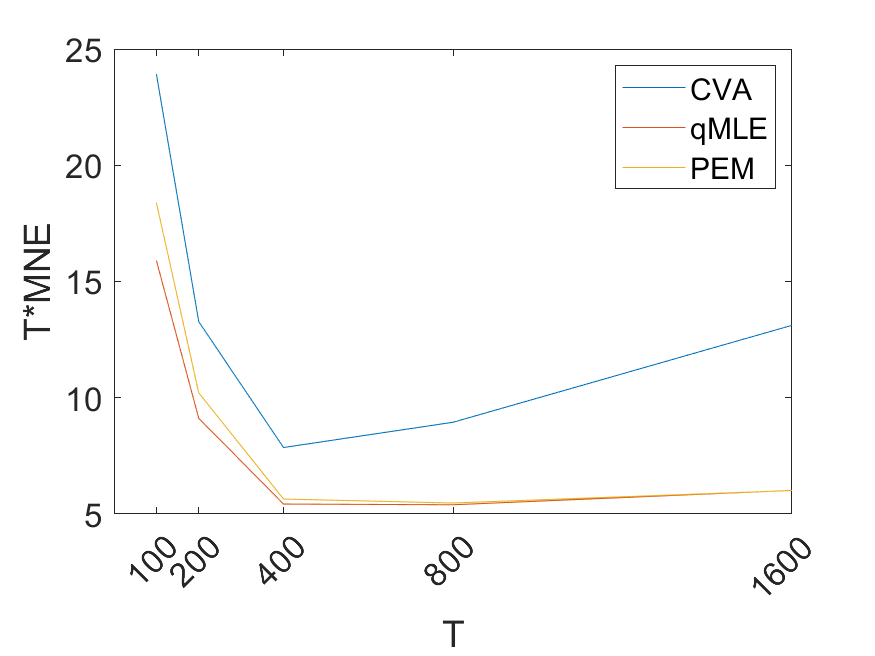
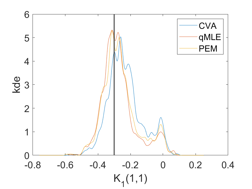
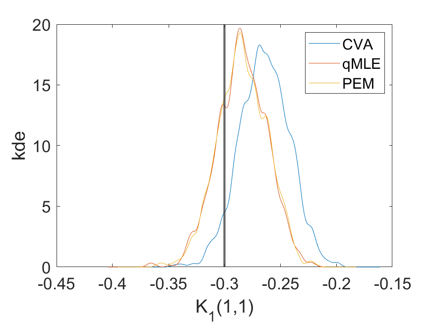
(a)	(b)	(c)

Figure 1: (a) Mean squared norm of impulse response estimation error times sample size. (b) Density estimate of estimates of $K_{1}(1,1)$ for $T=200$. (c) Density estimate of estimates of $K_{1}(1,1)$ for $T=1600$.

While the impulse response estimates for the large sample size appear to be Gaussian distributed, this is not the case for all system dependent quantities. Figure 2 (a) and (b) provides density estimates for the estimate of the trace of $\underline{A}=A-BC$. For $\underline{A}_{\circ}=A_{\circ}-B_{\circ}C_{\circ}=I_{2}\in{\mathbb{R}}^{2}$ the trace equals $2$. The minimum-phase assumption implies that all eigenvalues need to be smaller than 1 in modulus. Hence $\mbox{tr}(\underline{A})\leq 2$ must hold for all estimates from qMLE and is likely to hold for PEM estimates. This is visible for both sample sizes. The trace for qMLE and PEM clearly is not Gaussian distributed with a strong discrete component at $2$. For CVA the situation is different: The bias results in smaller values at both sample sizes and the estimates appear to be well represented as a normal distribution around the biased value.

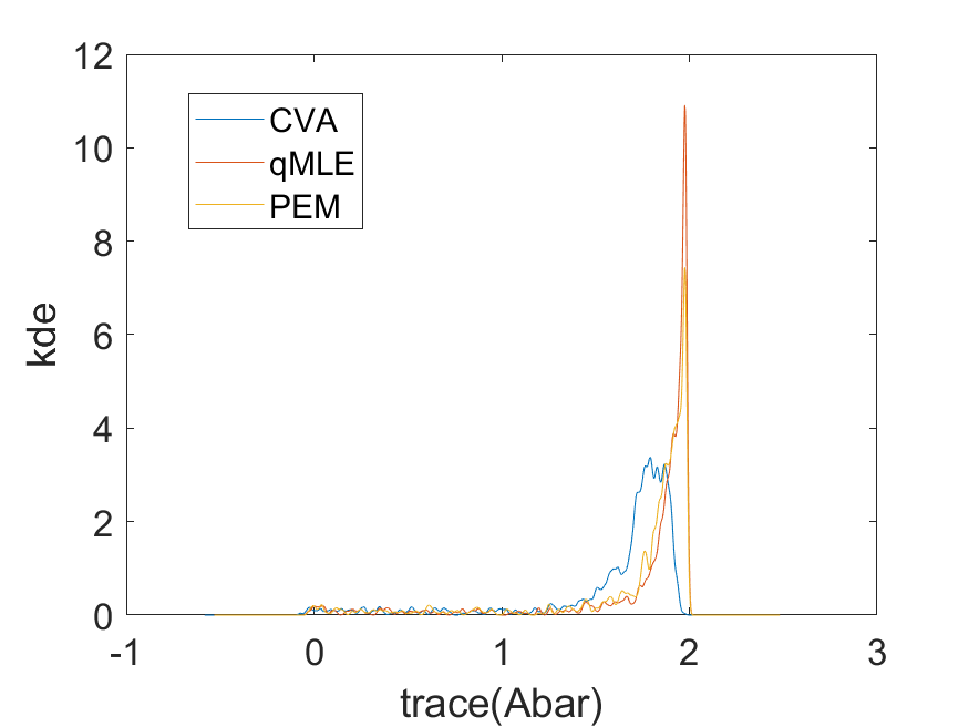
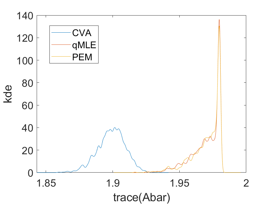
(a)	(b)
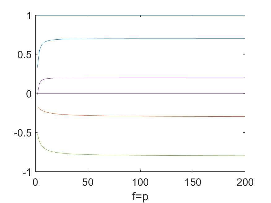
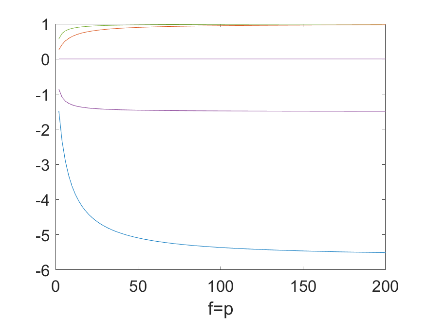
(c)	(d)

Figure 2: Density estimate of the estimated trace of $\underline{A}$ for $T=200$ (a) and $T=1600$ (b). For numerical reasons the barrier is located for eigenvalue equal to 0.99. (c): Dependence of $(A_{p},B_{p},C_{p})$ on $p$. (d): Scaled deviations of $(A_{p},B_{p},C_{p})$ from $(A_{\circ},B_{\circ},C_{\circ})$ as a function of $p$.

The lower row of plots in Figure 2 demonstrates the size of the bias in the CVA quantities $(A_{p},B_{p},C_{p})$ calculated using the CVA algorithm using the true covariances in place of their estimates. The evaluations in the example suggest that the bias in $A_{p}$ is of order $O(p^{-2})$, while the bias in the entries of $B_{p}$ is of order $O(p^{-1})$. Figure 2 (c) provides a plot of the entries in the system as a function of $f=p$, while (d) scales by multiplying the deviations $A_{p}-A_{\circ}$ by $p^{2}$ and the deviations in the remaining system matrices by $p$. We observe the decrease in the bias, which according to the scaled plot (d) is of the order given in the example.

5 Conclusions

In this paper we show that working with first differences does not invalidate consistency for CVA. This is a relief in situations where one is not sure about the existence of cointegrating relations or the presence of all seasonal unit roots, when working with (seasonal) differences rather than the original measurements.

Inference, on the other hand, gets more complicated as the asymptotic distribution in a situation, where some of the variables are over-differenced, is not known, contrary to the case of no over-differencing. Our results show that in this situation the estimates suffer from a relatively large bias term preventing the usual $\sqrt{T}$ asymptotic normality and hence inference for subspace estimates is non-standard in these cases.

The results imply that also higher order of differencing can be dealt with using exactly the same methods, but making things even worse. In such situations consistency of CVA estimators of the impulse response sequence again follows for $p$ increasing sufficiently slow.

However, in all these cases the rate of consistency is slower than $1/\sqrt{T}$. Hence the main message of this paper is to prefer the original, un-differenced time series for inference.

Declarations

• Funding: This research was funded by the Deutsche Forschungsgemeinschaft (DFG, German Research Foundation - Projektnummer 469278259) which is gratefully acknowledged.

• Conflict of interest/Competing interests: The author declares that there are no competing interests.

Proof of Lemma 1

Theorem 2 of Palma and Bondon (2003) deals with the univariate case and provides the lower bound for the eigenvalues of $\Gamma_{p}$. The spectral zeros in that theorem can be at arbitrary locations with different multiplicity. The order of the smallest eigenvalue then depends on the largest multiplicity. In the current case we only have simple eigenvalues such that $d_{1}=-1$ there.
In our situation we have

$$f(\omega) =\frac{1}{2\pi}k(e^{i\omega})\Sigma k(e^{i\omega})^{*}$$

$$\geq M\begin{pmatrix}(1-e^{i\omega})I_{c}&0\\ 0&I_{s-c}\end{pmatrix}\begin{pmatrix}(1-e^{-i\omega})I_{c}&0\\ 0&I_{s-c}\end{pmatrix}M^{\prime}\underline{c}$$

$$\geq|1-e^{i\omega}|^{2}\frac{\underline{c}}{2}I_{s}$$

for some real $\underline{c}$, since $|1-e^{i\omega}|^{2}\leq 2$ and $\frac{1}{2\pi}M^{\prime}\tilde{k}(e^{i\omega})\Sigma\tilde{k}(e^{i\omega})^{*}M\geq\underline{c}I_{s}$ due to the invertibility of $\tilde{k}(z)$ assumed in Assumption 1.
The rest of the proof then follows exactly as in Palma and Bondon (2003). ∎

Proof of Theorem 1

Note that $\hat{\alpha}(p)=\langle Y_{t}^{+},Y_{t}^{-}\rangle\langle Y_{t}^{-},Y_{t}^{-}\rangle^{-1}$ is an autoregressive approximation of $Y_{t}^{+}$ by $Y_{t}^{-}$ if $p=f\tilde{p}$ for some integer $\tilde{p}$:

$$Y_{t}^{+}=\alpha(p)Y_{t}^{-}+U_{t}^{+}(p).$$

Poskitt (2006) Theorem 5 then implies that $\|\hat{\alpha}(p)-\alpha(p)\|_{2}^{2}=O(p^{5}Q_{T}^{2})$ using $(\lambda_{min}(\Gamma_{p}))^{-1}=O(p^{2})$ from Lemma 1. The proof of this result in Poskitt (2006) can be easily extended to the case of general $p$ in our setting: the argument uses $\langle y_{t+j},y_{t-k}\rangle-{\mathbb{E}}y_{t-j}y_{t-k}^{\prime}=O(Q_{T})$ and uniform (in $p$) bounds on the norm of $\Gamma_{p}$. Here $Q_{T}=\sqrt{(\log T)/T}$ is used. Both obviously hold also for sub-matrices.

Clearly $\alpha(p)=\mathcal{O}_{f}\mathcal{K}_{p}$ is of rank $n$ as $\mathcal{E}_{f}E_{t}^{+}$ is orthogonal to $Y_{t}^{-}$. CVA then uses a SVD of $\hat{\Xi_{f}}\hat{\alpha}(p)\langle Y_{t}^{-},Y_{t}^{-}\rangle^{1/2}$ or equivalently the SVD of

$$\hat{\Xi_{f}}\hat{\alpha}(p)\langle Y_{t}^{-},Y_{t}^{-}\rangle\hat{\alpha}(p)^{\prime}(\hat{\Xi_{f}})^{\prime}$$

to obtain a rank $n$ approximation where $\hat{\Xi_{f}}=\langle Y_{t}^{+},Y_{t}^{+}\rangle^{-1/2}$ (the square root denotes the Cholesky decomposition). Due to the uniform convergence of the sample covariances we obtain $\hat{\Xi_{f}}-\Xi_{f}=O(Q_{T})$ for fixed $f$ since the Cholesky factorization is differentiable for positive definite matrices.

Now $\|\alpha(p)\|_{\infty}=O(p)$ ($\|.\|_{\infty}$ denoting the row-sum norm) as can be seen, for example, from the Levinson-Whittle algorithm (see Hannan and Deistler (1988), p. 218). It follows that $\|\alpha(p)\|_{1}=O(1)$ (column-sum norm, here equivalent to maximum entry due to finite $f$), $\alpha(p){\mathbb{E}}Y_{t}^{-}(Y_{t}^{-})^{\prime}={\mathbb{E}}Y_{t}^{+}(Y_{t}^{-})^{\prime}$ and $\|\alpha(p)\|_{2}=O(\sqrt{p})$. Consequently

$$\hat{\alpha}(p)\langle Y_{t}^{-},Y_{t}^{-}\rangle\hat{\alpha}(p)^{\prime}-\alpha(p){\mathbb{E}}Y_{t}^{-}(Y_{t}^{-})^{\prime}\alpha(p)^{\prime}=O(p^{5/2}Q_{T}).$$

The properties of the SVD then imply $\|\hat{\mathcal{O}_{f}}-\mathcal{O}_{f}\|_{2}=O(p^{5/2}Q_{T})$ which in turn leads to $\|\hat{\mathcal{K}_{p}}-\mathcal{K}_{p}\|_{2}=O(p^{5/2}Q_{T})$: Key here is the differentiable dependence of the eigenspace to an eigenvalue on the matrix, see Chatelin (1993). This applies here as $\mathcal{O}_{f}$ spans the orthocomplement of the eigenspace to eigenvalue zero. The convergence for $\hat{\mathcal{O}_{f}}$ then requires fixing a basis of this space which is achieved by $S_{f}\mathcal{O}_{f}=I_{n}$. We then use the same normalisation for $\hat{\mathcal{O}_{f}}$ such that $S_{f}\hat{\mathcal{O}_{f}}=I_{n}$ to obtain $\|\hat{\mathcal{O}_{f}}-\mathcal{O}_{f}\|_{2}=O(p^{5/2}Q_{T})$. As $\mathcal{O}_{f}^{\prime}\mathcal{O}_{f}\geq I_{s}$ we have with $\mathcal{K}_{p}=(\mathcal{O}_{f}^{\prime}\mathcal{O}_{f})^{-1}\mathcal{O}_{f}^{\prime}\alpha(p)$ and $\hat{\mathcal{K}_{p}}=(\hat{\mathcal{O}_{f}}^{\prime}\hat{\mathcal{O}_{f}})^{-1}\hat{\mathcal{O}_{f}}^{\prime}\hat{\alpha}(p)$ that $\|\hat{\mathcal{K}_{p}}-\mathcal{K}_{p}\|_{2}=O(p^{5/2}Q_{T})$.

The remainder of the proof then follows from providing error bounds for terms involving

$$\hat{x}_{t}(p)-x_{t}(p)=(\hat{\mathcal{K}_{p}}-\mathcal{K}_{p})Y_{t}^{-}.$$

For example,

$$\langle\hat{x}_{t},\hat{x}_{t}\rangle = \langle\hat{x}_{t}-x_{t}(p),\hat{x}_{t}\rangle+\langle x_{t}(p),\hat{x}_{t}-x_{t}(p)\rangle+\langle x_{t}(p),x_{t}(p)\rangle$$

$$= (\hat{\mathcal{K}_{p}}-\mathcal{K}_{p})\langle Y_{t}^{-},Y_{t}^{-}\rangle\hat{\mathcal{K}_{p}}^{\prime}+\mathcal{K}_{p}\langle Y_{t}^{-},Y_{t}^{-}\rangle(\hat{\mathcal{K}_{p}}-\mathcal{K}_{p})^{\prime}+\langle x_{t}(p),x_{t}(p)\rangle$$

$$= (\hat{\mathcal{K}_{p}}-\mathcal{K}_{p}){\mathbb{E}}Y_{t}^{-}x_{t}(p)^{\prime}+{\mathbb{E}}x_{t}(p)(Y_{t}^{-})^{\prime}(\hat{\mathcal{K}_{p}}-\mathcal{K}_{p})^{\prime}+\langle x_{t}(p),x_{t}(p)\rangle+o(p^{5/2}Q_{T})$$

$$= \langle x_{t}(p),x_{t}(p)\rangle+O(p^{5/2}Q_{T})$$

where the next to last error bound follows from replacing estimates with limits. $\|{\mathbb{E}}Y_{t}^{-}x_{t}(p)^{\prime}\|_{2}=O(1)$ due to the assumed stability. All evaluations are simple and hence omitted.

These arguments show that uniformly for $0<p\leq H_{T}$ the difference between the estimates using $\hat{x}_{t}$ and using $x_{t}(p)$ is of order $O(p^{5/2}Q_{T})$.

Considering $\langle x_{t}(p),x_{t}(p)\rangle-{\mathbb{E}}x_{t}(p)x_{t}(p)^{\prime}$ we see that

$$\alpha(p)(\langle Y_{t}^{-},Y_{t}^{-}\rangle-\Gamma_{p})\alpha(p)^{\prime}=O(p^{2}Q_{T})$$

since $\|\alpha(p)\|_{1}=O(1)$. This holds uniformly in $p<H_{T}$. Similar results show that $\langle\hat{x}_{t+1},\hat{x}_{t}\rangle-{\mathbb{E}}x_{t+1}(p)x_{t}(p)^{\prime}=O(p^{5/2}Q_{T}),\langle y_{t},\hat{x}_{t}\rangle-{\mathbb{E}}y_{t}x_{t}(p)^{\prime}=O(p^{5/2}Q_{T})$, $\langle y_{t},\hat{x}_{t+1}\rangle-{\mathbb{E}}y_{t}x_{t+1}(p)^{\prime}=O(p^{5/2}Q_{T})$. Consequently we get

$$\max\{\|\hat{A}-A_{p}\|_{2},\|\hat{B}-B_{p}\|_{2},\|\hat{C}-C_{p}\|_{2}\}=O(p^{5/2}Q_{T})=o(1)$$

for $p\leq H_{T}$.

To investigate $A_{p}-A_{\circ}$, for example, the difference of the second moments such as ${\mathbb{E}}x_{t}(p)x_{t}(p)^{\prime}-{\mathbb{E}}x_{t}x_{t}^{\prime}$ is essential: For these convergence to zero follows since ${\mathbb{E}}\delta x_{t}(p)(\delta x_{t}(p))^{\prime}\to 0$, as the approximation error converges to zero, compare Lemma 1 of (Poskitt, 2006). This finishes the proof.

Proof of Theorem 2

The proof follows the structure of the proof of asymptotic normality in Bauer, Deistler and Scherrer (1999). It uses two facts:

1. The covariance sequence estimators $\hat{\gamma}_{j}=\langle y_{t},y_{t-j}\rangle,j=0,1,...,f+p$ are asymptotically normally jointly for fixed $f,p$ according to the arguments around Lemma 4.3.4 of Hannan and Deistler (1988).

2. The estimators of the system matrices in an appropriate overlapping form can be written as a nonlinear continuously differentiable mapping of the covariance sequence estimators.

The result then follows from the Delta rule.
Since 1. follows from Hannan and Deistler (1988), we only need to investigate 2.: In this respect note that this point is used also in Bauer, Deistler and Scherrer (1999).
Examine the CVA approach to construct the non-linear mapping:

• Regression of $Y_{t}^{+}$ onto $Y_{t}^{-}$ is a nonlinear mapping of the covariance sequence. The estimate can be written as $\hat{\beta}_{f,p}=\langle Y_{t}^{+},Y_{t}^{-}\rangle\langle Y_{t}^{-},Y_{t}^{-}\rangle^{-1}$. This is continuously differentiable, if $\langle Y_{t}^{-},Y_{t}^{-}\rangle$ is non-singular. Since $\lambda_{min}(\Gamma_{p})>0$ for fixed $p$ according to Lemma 1, continuous differentiability holds.

• The second step is the calculation of the SVD involving weighting matrices. The weighting matrices are Cholesky factors of estimated second moments like $\langle Y_{t}^{-},Y_{t}^{-}\rangle$. Again the weights are continuously differentiable functions of the covariance sequence. The SVD is equivalent to an eigenvalue decomposition of the squared matrix. For eigenvalue decompositions it is known that the column space is an analytic function of the matrix that is decomposed (see Chatelin, 1993).

• Then $\hat{}\mathcal{K}_{p}=\hat{\mathcal{O}_{f}}^{\dagger}\hat{\beta}_{f,p}$ is calculated. Since $\hat{\mathcal{O}_{f}}$ depends continuously differentiable on the covariance sequence the same holds for $\hat{}\mathcal{K}_{p}$.

• The remaining steps of the algorithm are regressions, that depend continuously differentiable on the second moment matrices.

This shows the theorem. Note that the expressions in Chatelin (1993) even would allow for the derivation of expressions for the asymptotic variance. Again, given the strong bias it is questionable, if such expressions are of much value.

References

- Bauer (2005) \bibinfoauthorBauer, D., \bibinfoyear2005. \bibinfotitleEstimating linear dynamical systems using subspace methods. \bibinfojournalEconometric Theory \bibinfovolume21. pp. \bibinfopages181–211.
- Bauer (2019) \bibinfoauthorBauer, D., \bibinfoyear2019. \bibinfotitlePeriodic and seasonal (co-) integration in the state space framework. \bibinfojournalEconomics Letters \bibinfovolume174. pp. \bibinfopages165–168.
- Bauer and Buschmeier (2021) \bibinfoauthorBauer, D., \bibinfoauthorBuschmeier, R., \bibinfoyear2021. \bibinfotitleAsymptotic properties of estimators for seasonally cointegrated state space models obtained using the CVA subspace method. \bibinfojournalEntropy \bibinfovolume23. \bibinfopages436.
- Bauer, Deistler and Scherrer (1999) \bibinfoauthorBauer, D., \bibinfoauthorDeistler, M., \bibinfoauthorScherrer, W., \bibinfoyear1999. \bibinfotitleConsistency and asymptotic normality of some subspace algorithms for systems without observed inputs. \bibinfojournalAutomatica \bibinfovolume7. \bibinfopages1243–1254.
- Bauer and Wagner (2021) \bibinfoauthorBauer, D., \bibinfoauthorWagner, M., \bibinfoyear2012. \bibinfotitleA state space canonical form for unit root processes. \bibinfojournalEconometric Theory \bibinfovolume28. pp. \bibinfopages1313–1349.
- Chatelin (1993) \bibinfoauthorChatelin, F., \bibinfoyear1993. \bibinfotitleEigenvalues of Matrices. \bibinfopublisherJohn Wiley & Sons.
- Funovits (2024) \bibinfoauthorFunovits, B., \bibinfoyear2024. \bibinfotitleIdentifiability and estimation of possibly non-invertible SVARMA Models: The normalised canonical WHF parametrisation. \bibinfojournalJournal of Econometrics \bibinfovolume241, \bibinfopages105766.
- Hannan and Deistler (1988) \bibinfoauthorHannan, E.J., \bibinfoauthorDeistler, M., \bibinfoyear1988. \bibinfotitleThe Statistical Theory of Linear Systems. \bibinfopublisherJohn Wiley, \bibinfoaddressNew York.
- Larimore (1983) \bibinfoauthorLarimore, W.E., \bibinfoyear1983. \bibinfotitleSystem Identification, reduced order filters and modeling via canonical variate analysis, \bibinfoaddressPiscataway, NJ. pp. \bibinfopages445–451.
- Palma and Bondon (2003) \bibinfoauthorPalma, W., \bibinfoauthorBondon, P., \bibinfoyear2003. \bibinfotitleOn the Eigenstructure of Generalized Fractional Processes. \bibinfojournalStatistics and Probability Letters \bibinfovolume65, \bibinfopages93–101.
- Pötscher (1991) \bibinfoauthorPötscher, B., \bibinfoyear1991. \bibinfotitleNoninvertibility and pseudo-maximum likelihood estimation of misspecified ARMA models. \bibinfojournalEconometric Theory \bibinfovolume7, \bibinfopages435–449.
- Poskitt (2006) \bibinfoauthorPoskitt, D.S., \bibinfoyear2006. \bibinfotitleAutoregressive approximation in nonstandard situations: the fractionally integrated and non-nivertible case. \bibinfojournalAnnals of Institute of Statistical Mathematics \bibinfovolume59, \bibinfopages697–725.