Statistical modeling of categorical trajectories with multivariate functional principal components
Abstract
There are many examples in which the statistical units of interest are samples of a continuous time categorical random process, that is to say a continuous time stochastic process taking values in a finite state space. Without loosing any information, we associate to each state a binary random function, taking values in , and turn the problem of statistical modeling of a categorical process into a multivariate functional data analysis issue. The (multivariate) covariance operator has nice interpretations in terms of departure from independence of the joint probabilities and the multivariate functional principal components are simple to interpret. Under the weak hypothesis assuming only continuity in probability of the trajectories, it is simple to build consistent estimators of the covariance kernel and perform multivariate functional principal components analysis. The sample paths being piecewise constant, with a finite number of jumps, this a rare case in functional data analysis in which the trajectories can be observed exhaustively. The approach is illustrated on a data set of sensory perceptions, considering different gustometer-controlled stimuli experiments. We show how it can be easily extended to analyze experiments, such as temporal check-all-that-apply, in which two states or more can be observed at the same time.
Keywords : categorical functional data, continuous time categorical processes, dimension reduction, discontinuous trajectories, sensometrics, temporal dominance of sensations, temporal check all that apply
1 Introduction
A lot of attention has been paid in the statistical literature over the last decades to develop tools dedicated to the analysis and modeling of functional data, considering random trajectories defined on an interval of time and taking values in , at each (see for example [11] and [16] for recent reviews of the literature). Much less attention has been given to the case in which the trajectories take values in a finite set of elements that are not necessarily numbers, that is to say when is replaced by the finite set , with cardinality .
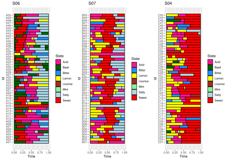
There are many examples in which the statistical units of interest are samples of a continuous time random categorical process : in a pioneer work on demographic studies, Deville [8] extended the notion of multiple correspondence analysis to continuous time correspondence analysis in order to analyze the time evolution of the ”marital status” of a sample of women over the period . The trajectories related to the marital status take values in a state space with states (divorced, married, single, widowed). Recent examples of statistical analysis of individual categorical trajectories are found in food science, a domain in which it is of great interest to get information about the temporal perception of aliments to understand the perception mechanisms. Of particular interest is the Temporal Dominance of Sensations (TDS) approach which consists in choosing sequentially attributes, among a list composed of predefined items, describing a food product over tasting. The chosen states correspond to the most striking perception at a given time and the results of TDS experiments, after time normalization, can be represented via barplots as in Figure 1. The technique developed by [8], also called qualitative harmonic analysis (see [9]) or categorical functional data analysis (CFDA) is now available in R, package cfda (see [22]) and can be used to analyze such kind of data. Even if the CFDA approach can be very powerful by encoding categorical trajectories into a sequence of real components (see [20] for an illustration in sensory analysis), the interpretation of the results in terms of individual trajectories is often delicate.
Statistical approaches based on Markov processes and their extensions (see [19] for an overview and [18] for an introduction to semi-Markov processes) can be useful to fit the law of the trajectories at the population level and to provide a simple representation of the dynamics via the graph of transitions between states. Considering parametric distributions for the sojourn time in the different states also allows to deal with maximum likelihood estimation techniques, permitting to build two-sample tests to compare two populations (e.g two food products or two categories of consumers (see [6]) as well as model-based clustering, considering mixtures of semi-Markov processes (see [5]). A major drawback of this approach is that it is not well suited for analyzing data at the individual level, and the Markovian assumption is often too simplistic to properly fit real data. Additionally, it is difficult to apply when more than one state can be present simultaneously (see the TCATA experiment in Section 4.2), as this requires drastically increasing the number of system states to to account for all possible combinations.
In this work, we introduce another point of view and associate to each state , for , a random trajectory , taking value 1 when state is observed at time and zero else. The information given by a categorical trajectory is equivalent to the information given by the binary 0-1 trajectories .
One could consider such trajectories as compositional data evolving over time (see [1] for a seminal paper and [12] for a recent review on compositional data analysis). A major difficulty to deal with compositional data approaches in our framework is due to the fact that we deal with individual trajectories so that, at each instant , individual observations, among , have value 0. In other words, at each instant , all the observed units are on the vertices of the simplex, so that usual logarithmic transforms cannot apply directly.
Our approach is based on the optimal approximation, according to the distance, to such 0-1 trajectories in a small dimension functional space. This leads us to consider the multivariate functional principal component analysis (MFPCA) of the multivariate functional vector . We show that it leads both to principal components that can be simply interpreted in terms of variations around the mean probability curve related to each state, and powerful tools able to reduce effectively the dimension of categorical functional data in a finite dimension vector space.
2 Notations and mathematical framework
To describe continuous time categorical trajectories, we consider the random element , with for all . We denote by , the probability of being in state at time and, for and , the joint probability
We associate to the random element , trajectories , , related to the occurrence of state , and defined as follows, if and otherwise. In other words, , for all , where is the indicator function. We clearly have
and
We suppose in the following that hypothesis is satisfied
ensuring that the trajectories are continuous in probability. Hypothesis prevents them to have too many jumps. Define the covariance functions and, for , . We remark that and , so that the terms out of the diagonal, when , can be related to a departure from independence.
Proposition 2.1.
Under hypothesis , we have for all ,
-
•
(resp. ) is continuous on (resp. on )
-
•
is continuous on , for all .
The proof of Proposition 2.1 is given in the Appendix. Note that the binary trajectories take values in the Hilbert space equipped with the usual inner product, denoted by , and norm . Denote by the cross-covariance operator between and . It is the integral operator with kernel function ,
| (1) |
Considering now simultaneously , we denote by the random vector of functions, that takes values in , the Hilbert space of dimensional vectors of functions in , equipped with the inner product
| (2) |
The weights that can be chosen by the statistician (see Remark 2 below and Section 4) are strictly positive. We denote by the expectation of , , and by the covariance operator. It satisfies, ,
| (3) | ||||
| (4) |
We denote by the corresponding (weighted) multivariate covariance function, with elements . We deduce from Proposition 2.1 and the multivariate version of Mercer’s theorem (see [7] or [14]) that there exists a set of orthonormal basis functions in , and corresponding eigenvalues such that
This leads to the following expansion of the covariance functions ,
| (5) |
It is not difficult to show that operator , defined in (3), is the integral operator with kernel function and . Furthermore,
The optimal linear expansion of in a dimensional vector space of , in terms of quadratic mean, is given by the truncated Karhunen-Loève expansion of ,
| (6) |
Our aim is to estimate and , for , in order to be able to capture the main variations of a categorical random function in a small dimensional vector space.
Remark 1.
The continuous time extension of correspondence analysis, named qualitative harmonic analysis and developed by [8] and [9] is based on the eigen decomposition of another integral operator, with a purpose that is not to expand the trajectories themselves in an ”optimal” way but to relate the states to numerical values at each instant . More precisely, the aim is to find an optimal encoding function minimizing the following criterion
subject to identifiability constraints for all and unit variance . A solution satisfies, for all , the integral operator equation (see equation (42) in [8]),
| (7) |
Departure from independence is evaluated via the ratio which is equal to one in case of independence. Denoting by the sequence eigenvalues of operator equation (7) and by the eigenfunction related to , we get a Mercer type expansion of the joint probabilities (see equation (43) in [8]),
| (8) |
This means that the optimal encoding approach considers implicitly a multiplicative point of view to expand the departure from independence of the joint probabilities whereas the optimal trajectory expansion studied in this article considers an additive point of view, as seen in (5).
Remark 2.
If the statistician wants to give the same importance to all the states, one reasonable option consists in choosing weights
| (9) |
setting to one the trace of the covariance operator of the binary (normalized) trajectory .
Remark 3.
Previous framework can be extended easily to experiments in which more than two states can be present simultaneously without increasing the cardinality of . If we replace by the hypothesis that the trajectories are continuous in probability, Proposition 2.1 remains true.
3 Sampling and estimators
Suppose now we have a sample of categorical trajectories observed over and taking values in . We define the vector of the corresponding binary trajectories, with . These trajectories are piecewise constant, with a finite number of jumps. It is a rare case in functional data analysis in which the trajectories can be observed exhaustively, that is to say for all time point .
We consider, for all and in , the empirical probabilities of occurrence and . We also consider the joint empirical probabilities , and define the estimators of the covariance functions
and
We deduce from (1), estimators of the cross-covariance operators and from (4), an estimator of . Note that in a more formal way, we can express
where the tensor product is defined as follows, for all belonging to . We can state the following consistency and asymptotic normality results which follows immediately from assumption . We denote by the spectral norm of linear operator induced by the norm in .
Proposition 3.1.
Suppose that hypothesis is fulfilled, as tends to infinity,
-
•
and almost surely,
-
•
and are asymptotically Gaussian.
4 Two illustrations in sensory analysis
The dataset used for both illustrations concerns sensory experiences. It is well documented in [3] and can be obtained from a public source. In each illustration fifty panelists took part in a tasting experiment and were asked to click on the sensation they perceived in real time from a list of descriptors. Computations were performed with the library MFPCA (see [13]) in the R language [23]. All codes are available on Github, https://github.com/Chemosens/ExternalCode/MFPCAWithCategoricalTrajectories.
When participants are instructed to click only on the dominant sensation, i.e. when only one perception can be observed at any given time, the protocol is called Temporal Dominance of Sensation” (TDS, see [21] for a reference article). When participants are asked to click on all the sensations they perceive in real time from the same list of descriptors, the protocol is called Temporal Check-All-That-Apply (TCATA, see [4] for a seminal article). Unlike the TDS protocol, several descriptors (or none at all) can be selected at any given time for TCATA experiments. The resulting data consists of binary trajectories linked to each state, with the value 0 when a descriptor is unclicked at time and 1 when it is clicked. The main difference between TCATA and TDS is that at each instant t, the sum of all binary trajectories can be different from 1 and take values in the set .
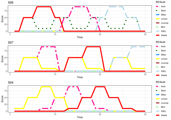
Ill all the experiments, the tasted temporal solution is controlled and delivered by a gustometer. Three controlled sensory signals (see Figure 2) were tasted by the panelists: S04 (Lemon, followed by Acid, and finally Sweet), S06 (Sweet, Acid, and finally Salty, with a continuous hint of Basil), and S07 (Acid, followed by Sweet, and finally Salty, with a continuous hint of Lemon). The descriptor list included Acid, Sweet, Lemon, Basil, and Salty, alongside distractors such as Mint, Licorice and Bitter, so that the categorical process has states.
The overall number of experiments is and time has been normalized to be for each experiment, resulting, for TDS, in the observed categorical trajectories drawn in Figure 1.
4.1 Temporal dominance of sensation (TDS) trajectories
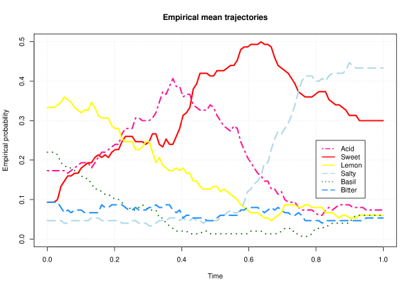
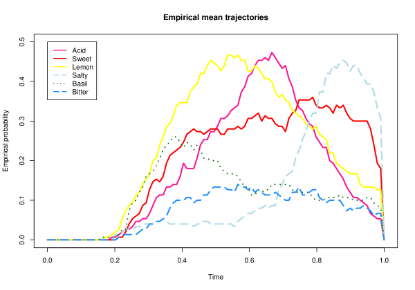
The estimated mean probability of perception are drawn in Figure 3, where we only present the states (Acid, Basil, Bitter, Lemon, Salty, Sweet) whose probability of occurrence is sufficiently large, that is to say such that . The most frequently observed states are Lemon at the beginning of the period, then Acid, Sweet and Salty at the end of the period.
| Acid | Basil | Bitter | Lemon | Licorice | Mint | Salty | Sweet | |
|---|---|---|---|---|---|---|---|---|
| 0.12 | 0.12 | 0.12 | 0.12 | 0.12 | 0.12 | 0.12 | 0.12 | |
| 0.02 | 0.06 | 0.05 | 0.02 | 0.21 | 0.60 | 0.03 | 0.01 | |
| 0.02 | 0.05 | 0.05 | 0.02 | 0.21 | 0.62 | 0.02 | 0.01 |
The influence of weighting schemes on the multivariate functional principal components
We consider different weighting schemes , modifying the geometry in via its inner product (2) and giving rise to different Karhunen-Loève expansions (6). These weights, normalized to sum up to one, are given in Table 1.
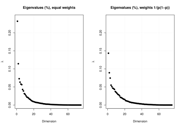
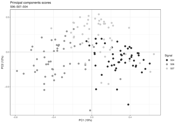
First, a multivariate FPCA of the trajectories , , considering equal weights has been performed, giving the same weight to all states . The first eigenvalue represents 23% of the total variance, whereas the second one represents 11% of the total variance, the third one 7% and the fourth one 6%. The decrease of the eigenvalues to zero is rather slow (see Figure 4), which is not so surprising since the trajectories are not continuous.
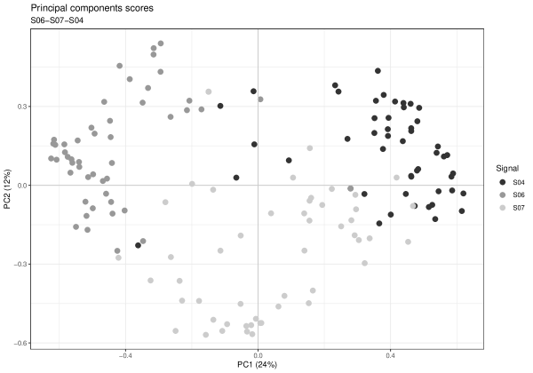
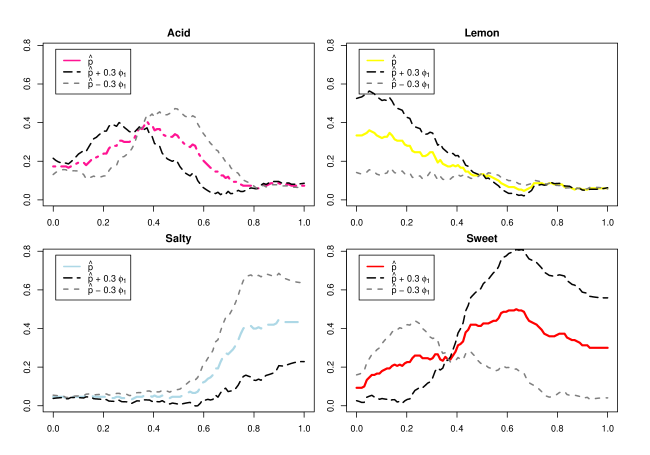
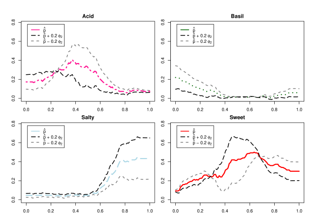
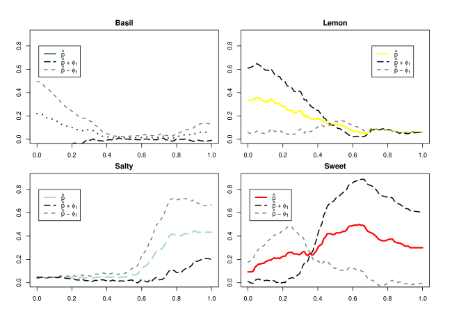
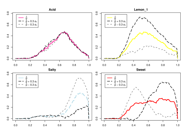
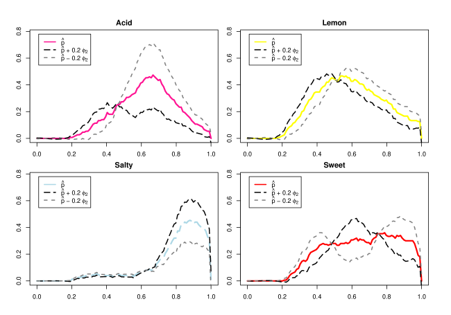
The estimated principal component scores , for are drawn in Figure 5, whereas the main variations around the mean functions, for the first two dimensions, are drawn in Figure 6 and Figure 7. For better interpretation and graphical representation, we only consider the components with the largest variations, that is to say with the largest values of , . Since, for each value of , , we can build the following indicator of importance of each category in dimension ,
| (10) |
with , and consider only the most important variables (see Table 2). This leads us to select for graphical representation of the eigenfunctions the states Acid, Lemon, Salty and Sweet for the first dimension and Acid, Basil, Salty and Sweet for the second dimension.
| dim 1 | dim 2 | dim 3 | dim 4 | dim 5 | |
|---|---|---|---|---|---|
| Acid | 0.08 | 0.26 | 0.42 | 0.29 | 0.31 |
| Basil | 0.04 | 0.07 | 0.00 | 0.04 | 0.03 |
| Bitter | 0.00 | 0.02 | 0.01 | 0.02 | 0.02 |
| Lemon | 0.10 | 0.02 | 0.48 | 0.13 | 0.25 |
| Licorice | 0.00 | 0.00 | 0.00 | 0.01 | 0.00 |
| Mint | 0.00 | 0.00 | 0.00 | 0.00 | 0.00 |
| Salty | 0.22 | 0.30 | 0.02 | 0.17 | 0.09 |
| Sweet | 0.56 | 0.34 | 0.06 | 0.35 | 0.30 |
The results are simple to interpret. For example, the black dots in Figure 5, corresponding to the S04 experiment, are characterized by a first principal component taking positive values, related, as seen in Figure 6, to a high probability of occurrence of Lemon and small probability of occurrence of Acid at the beginning of the period, and a high probability of occurrence of Sweet and a small probability of occurrence of Salty at the end of the period. This is the opposite situation for the S06 experiment whose observations (in grey dots) are related to a negative value of the first principal component. The light grey dots, that correspond to the S07 experiment are characterized by negative values of the second principal components. A look at Figure 7 indicates that the probability of perception of Sweet at the middle of the period and Salty at the end of the period is higher than the mean probability and the perception of Acid is higher at the beginning (between time 0 and 0.2) and then smaller. Negative values of the second component also correspond to a higher probability of occurrence of Basil at the beginning of the period, which is in agreement with experimental conditions S06 (see Figure 2).
We also consider weights, defined in (9) and equal to , that give more importance to the states whose average variance is small, that is to say that are often or very rarely observed (see in Table 1 for the numerical values). As noted in Remark 2, considering these weights lead to impose the covariance operators to have the same trace. As seen in Figure 4 on the right, the decrease to zero of the sequence of eigenvalues is slower compared to previous analysis with equal weights. We draw in Figure 8 the first two principal components.
| dim 1 | dim 2 | dim 3 | dim 4 | dim 5 | |
|---|---|---|---|---|---|
| Acid | 0.08 | 0.05 | 0.04 | 0.20 | 0.14 |
| Basil | 0.21 | 0.20 | 0.09 | 0.03 | 0.02 |
| Bitter | 0.00 | 0.02 | 0.14 | 0.07 | 0.19 |
| Lemon | 0.15 | 0.04 | 0.06 | 0.10 | 0.38 |
| Licorice | 0.01 | 0.02 | 0.01 | 0.56 | 0.14 |
| Mint | 0.00 | 0.22 | 0.56 | 0.00 | 0.03 |
| Salty | 0.19 | 0.36 | 0.05 | 0.00 | 0.04 |
| Sweet | 0.36 | 0.08 | 0.05 | 0.03 | 0.05 |
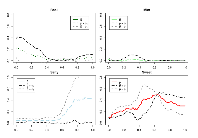
The examination of the most important states (see Table 3) in the first and second dimension does exhibit some little difference with the case of equal weights. First Basil appears to be influential in the first and in the second dimension, amplifying the probability of occurrence for negative value of the first component and positive value of the second component (see Figure 9 and Figure 10) even if the weight associated to this state is smaller in that unequal weights configuration compared to equal weights MFPCA. This makes it possible to identify, among the S06 tasting experiments, those in which the taste of basil was perceived. Another difference is the presence of Mint in the important variable, particularly on the second and third dimension whereas it was not present at all in the equal weights analysis.
4.2 Temporal Check All That Apply experiments (TCATA)
In the same dataset [3], the same gustometer signals (S04, S06, and S07) were also evaluated using the Temporal Check-All-That-Apply protocol but with another panel of fifty panelists.
The mean trajectories for each state are presented in Figure 11. We can remark that their value is equal to 0 in the time interval . This corresponds to a latency time between the start of the tasting and the first click. This latency time is removed in TDS to always have one descriptor selected, but it can be kept here. At the end of the tasting, all the descriptors are automatically unselected, which results in a zero mean value at time . The most frequently observed states are Lemon at the beginning of the period, followed by Acid, Sweet, and Salty at the end of the period, as in the TDS evaluations of the signals.
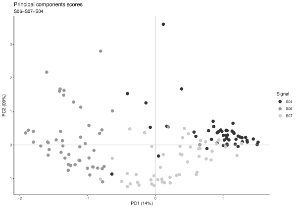
As the result of the TCATA experiment can be considered as a set of binary trajectories, MFPCA can be conducted on them. Here is an example with equal weights. The first eigenvalue represents 19% of the total variance, whereas the second one represents 12 % of the total variance (see Figure 12).

The estimated principal component scores are drawn in Figure 13, whereas the main variations around the mean functions, for the first two dimensions, are drawn in Figure 14 and Figure 15 for the descriptors selected in TDS. The points corresponding to the S04 experiment are characterized by a first principal component taking positive values, related, as seen in Figure 14 to a high probability of occurrence of Lemon in the middle of the tasting, a small probability of occurrence of Acid at the end of the period, and a high probability of occurrence of Sweet and a small probability of occurrence of Salty at the end of the period. Nothing appears on the first component for Acid perception. On the second component, the same points have negative scores, showing a high probability of Acid occurring after 0.5. The conclusions on the first two axes allow us to reconstruct the original signal (see Figure 2). The same reasoning can be applied to S06 and S07, which are well discriminated by the first two dimensions of the 1-2 map.
5 Concluding remark
The way, presented in this work, of reducing the dimension in a vector space of a panel of categorical trajectories allows for simple interpretation and comparison of individual trajectories. It is also direct to apply that methodology to other experimental protocols such as Temporal Check-All-That-Apply, in which and , , can be both equal to one at the same time , whereas this would require to increase considerably the number of states with the CFDA or Markov processes approaches. It can be easily extended to multivariate categorical trajectories, considering simultaneously, in our example, the three experiments made on the same panelists, that is to say . Finally, this methodology can be useful to build predictive models, such as scalar-on-categorical functional data regression models, permitting to use categorical trajectories as explanatory variables in statistical models. In our case it is easy to find which is the underlying tasting experiment, among S04, S06 and S07, with a simple linear or quadratic discriminant analysis based on the values of the principal components. This can also be useful to detect outlying trajectories in an automatic ways.
Acknowledgement
The Institut de Mathématiques de Bourgogne (UMR UB-CNRS 5584) receives support from the EIPHI Graduate School (contract ANR-17-EURE-0002).
Appendix A Proofs
Proof.
of Proposition 2.1
Remarking that almost surely, we deduce, by Theorem 1.3.6 in [24], that the trajectories are also continuous in the sense (or mean square continuous) when is true, that is to say
| (11) |
The continuity and is a consequence of Theorem 7.3.2 in [15] which states that the mean and covariance functions are continuous if and only if is mean-square continuous. To prove the continuity of , we note that for and in , we get thanks to the Cauchy-Schwarz inequality,
and we conclude using (11). ∎
Proof.
of Proposition 3.1
First note that equipped with the inner product is a separable Hilbert space.
We clearly have
so that all the moments of are finite. The proposition is then a direct consequence of Theorems 8.1.1 and 8.1.2 in [15] that are stated in general separable Hilbert spaces, considering the empirical mean and the empirical covariance operator ∎
References
- [1] Aitchison, J.: Principal component analysis of compositional data. Biometrika, 70, 57-65 (1983)
- [2] Ash, R.B., Gardner, M.F.: Topics in stochastic processes. Probability and Mathematical Statistics. New York - San Francisco - London: Academic Press (1975)
- [3] Béno, N., Nicolle, L., Visalli, M.: A dataset of consumer perceptions of gustometer-controlled stimuli measured with three temporal sensory evaluation methods. Data in Brief, 48, 109271. doi 10.1016/j.dib.2023.109271 (2023)
- [4] Castura, J. Antunez, L., Gimenez, A., Ares. G.: Temporal Check-All-That-Apply (TCATA): A novel dynamic method for characterizing products, Food Quality and Preference, 47A, 79–90 doi https://doi.org/10.1016/j.foodqual.2015.06.017 (2016)
- [5] Cardot, H., Frascolla, C., Schlich, P., Visalli, M.: Estimating finite mixtures of semi-Markov chains: an application to the segmentation of temporal sensory data. J. R. Stat. Soc., Ser. C, Appl. Stat. 68, 1281–1303 (2019)
- [6] Cardot, H., Frascolla, C.: Hypothesis testing for Panels of Semi-Markov Processes with parametric sojourn time distributions. J. Stat. Plann. Inference, 228, 59–79 (2024)
- [7] Chiou, J.M., Chen, Y.T., Yang, Y.F.: Multivariate functional principal component analysis: a normalization approach. Statistica Sinica, 24, 1571–1596 (2014)
- [8] Deville, J.C.: Analyse des données chronologiques qualitatives, Annales de l’INSEE, 45, 45-104 (1982)
- [9] Deville, J.C., Saporta, G.: Analyse harmonique qualitative, Data analysis and informatics, Proc. int. Symp., Versailles, 375-389 (1980)
- [10] Dauxois, J., Pousse, A., Romain, Y.: Asymptotic theory for the principal component analysis of a vector random function: Some applications to statistical inference. Journal of Multivariate Analysis, 12, 136–154 (1982)
- [11] Gertheiss, J., Rügamer, D., Liew, B. X. W., Greven, S.,: Functional Data Analysis: An Introduction and Recent Developments. Biometrical Journal, 66, e202300363 (2024)
- [12] Greenacre, M.: Compositional Data Analysis. Annu. Rev. Stat. Appl., 8, 271–299 (2021)
- [13] Happ, C.: MFPCA Multivariate Functional Principal Component Analysis. R package version 1.3-10 (2022)
- [14] Happ, C., Greven, S.: Multivariate functional principal component analysis for data observed on different (dimensional) domains. J. Am. Stat. Assoc., 113, 649–659 (2018)
- [15] Hsing, T., Eubank, R. : Theoretical foundations of functional data analysis, with an introduction to linear operators. Wiley Ser. Probab. Stat. Hoboken, NJ: John Wiley & Sons (2015)
- [16] Koner, S., Staicu, A.M : Second-Generation Functional Data. Annu. Rev. Stat. Appl., 10, 547-572 (2023)
- [17] Lecuelle, G., Visalli, M., Cardot, H., Schlich, P.: Modeling temporal dominance of sensations with semi-Markov chains. Food Quality and Preferences, 67, 59-66 (2018).
- [18] Limnios, N., Oprişan, G.: Semi-Markov processes and reliability. Stat. Ind. Technol., Basel: Birkhäuser (2001)
- [19] Lindsey, J.K (2012) Statistical analysis of stochastic processes in time. Camb. Ser. Stat. Probab. Math., Vol. 14, Cambridge: Cambridge University Press
- [20] Peltier, C., Visalli, M., Schlich, P. and Cardot, H.: Analyzing Temporal Dominance of Sensations data with Categorical Functional Data Analysis, Food Quality and Preference, 109. doi: 10.1016/j.foodqual.2023.104893 (2023)
- [21] Pineau, N., Schlich, P., Cordelle, S., Mathonnière, C., Issanchou, S., Imbert, A. Temporal Dominance of Sensations: Construction of the TDS curves and comparison with time-intensity. Food Quality and Preference, 20, 450-455, (2009).
- [22] Preda C, Grimonprez Q, Vandewalle V.: Categorical Functional Data Analysis. The cfda R Package. Mathematics 9(23):3074. doi :10.3390/math9233074 (2021)
- [23] R Core Team: R: A Language and Environment for Statistical Computing, R Foundation for Statistical Computing, Vienna, Austria, (2024)
- [24] Serfling, R.J.: Approximation theorems of mathematical statistics, Wiley Ser. Probab. Math. Stat., John Wiley & Sons, Hoboken, NJ (1980)