Towards Principled Multi-Agent Task Agnostic Exploration

Abstract

In reinforcement learning, we typically refer to task-agnostic exploration when we aim to explore the environment without access to the task specification a priori. In a single-agent setting the problem has been extensively studied and mostly understood. A popular approach cast the task-agnostic objective as maximizing the entropy of the state distribution induced by the agent’s policy, from which principles and methods follows. In contrast, little is known about task-agnostic exploration in multi-agent settings, which are ubiquitous in the real world. How should different agents explore in the presence of others? In this paper, we address this question through a generalization to multiple agents of the problem of maximizing the state distribution entropy. First, we investigate alternative formulations, highlighting respective positives and negatives. Then, we present a scalable, decentralized, trust-region policy search algorithm to address the problem in practical settings. Finally, we provide proof of concept experiments to both corroborate the theoretical findings and pave the way for task-agnostic exploration in challenging multi-agent settings.

1 Introduction

Multi-Agent Reinforcement Learning (MARL, Albrecht et al., 2024) recently showed promising results in learning complex behaviors, such as coordination and teamwork (Samvelyan et al., 2019), strategic planning in the presence of imperfect knowledge (Perolat et al., 2022), and trading (Johanson et al., 2022). Just like in single agent RL, however, most of the efforts are focused on tabula rasa learning, that is, without exploiting any prior knowledge gathered from offline data and/or policy pre-training. Despite its generality, learning tabula rasa hinders MARL from addressing real-world situations, where training from scratch every time is slow, often expensive, and most of all unnecessary (Agarwal et al., 2022). In this regard, some progress has been made on techniques specific to the multi-agent setting, ranging from ad hoc teamwork (Mirsky et al., 2022) to zero-shot coordination (Hu et al., 2020).

In single-agent RL, task-agnostic exploration, such as maximizing an entropy measure over the state space, was shown to be a useful tool for policy pre-training (Hazan et al., 2019; Mutti et al., 2021) and data collection for offline learning (Yarats et al., 2022). Recently, the potential of entropy objectives in MARL was empirically corroborated by a plethora of works (Liu et al., 2021a; Zhang et al., 2021; Xu et al., 2024) investigating entropic reward-shaping techniques to boost exploration. Yet, to the best of our knowledge, task-agnostic exploration has never been investigated for multi-agent scenarios explicitly, and, thus, the problem is far from being solved. Let us think of an illustrative example that highlights the central question of this work: multiple autonomous robots deployed in a collapsed building for a rescue operation mission. The robots’ main goal is to explore a large area to find and rescue injured humans, where exploration may involve coordinating with others to access otherwise inaccessible areas. Arguably, trying to enforce all robots to explore the entire area is inefficient and unnecessary. On the other hand, if everyone is focused on their own exploration, any incentive to collaborate with each other may disappear, especially when coordinating comes at a cost. Clearly, a third option is needed. Thus, many questions naturally arise: (i) How can task-agnostic exploration be defined in MARL? (ii) Are different formulations related in some way and when crucial differences emerge? (iii) How can we explicitly address multi-agent task-agnostic exploration in practical scenarios?

In this paper, we first provide a principled characterization of task-agnostic exploration in multi-agent settings by showing that the problem can take different, yet related, formulations. Specifically, the demarcation line is drawn by whether the agents are trying to jointly explore the space, or they neglect the presence of others and explore in a disjoint fashion, or, finally, whether they care of being able to explore the space together but as independent components of a mixture. We link these cases to three distinct objectives, each of them with specific pros and cons, and possibly leading to different behaviors. First, we formally show that these objectives are strictly related and enjoy similar behaviors in the ideal case of evaluating the agent’s performance over infinite realizations (or trials). Then, we shift the attention to the more practical scenario of reaching good performance over a handful, or even just one, trial. This is motivated by the fact that, even if we have access to a simulator to train our policies on many realizations, we often get to deploy them in a fair but limited amount of realizations. Interestingly, we show that different objectives enjoy rather different theoretical behaviors when optimized in such settings. Furthermore, we address the problem of how to optimize them, by introducing a decentralized multi-agent policy optimization algorithm, called Trust Region Pure Exploration (TRPE), explicitly addressing task-agnostic exploration over finite trials. Additionally, we test the algorithm on an illustrative proof of concept, showing its ability to optimize the objectives of interest, and, more importantly, showing how the diverse landscape of objectives turns out to be crucial for allowing effective coordinated exploration over short time-horizons. In particular, we show how optimizing for diverse exploration is not only crucial in practical scenarios, but is perhaps the only way to get relevant outcomes. We strengthen this claim by showing that this superiority is reflected in a higher effectiveness of policy pre-training for sparse-reward multi-agent tasks as well.

Contributions.

Throughout the paper, we make the following contributions:

• We introduce a novel class of decision making problems, called Convex Markov Games, and use them to extend the task-agnostic exploration problem to multi-agent settings (Section 3);

• We provide a theoretical characterization of the task-agnostic exploration problem, showing how the possible objectives are linked, and in what they are different (Section 4);

• We design a decentralized trust-region policy search algorithm able to address the exploration task in its most practical formulation (Section 5);

• We report empirical results that confirm the effectiveness of the algorithm in optimizing for their own objectives while highlighting the crucial differences of the different objectives. We showcase the limitations of more common objectives and the potentials of newly established mixture ones (Section 6).

2 Preliminaries

In this section, we introduce the most relevant background and the basic notation.

Notation.  In the following, we denote $[N]:=\{1,2,\ldots,N\}$ for a constant $N<\infty$. We denote a set with a calligraphic letter $\mathcal{A}$ and its size as $|\mathcal{A}|$. For a (finite) set $\mathcal{A}=\{1,2,\dots,i,\dots\}$, we denote with $-i=\mathcal{A}/\{i\}$ the set of all its elements out of the $i$-th one. We denote $\mathcal{A}^{T}:=\times_{t=1}^{T}\mathcal{A}$ the $T$-fold Cartesian product of $\mathcal{A}$. The simplex on $\mathcal{A}$ is denoted as $\Delta_{\mathcal{A}}:=\{p\in[0,1]^{|\mathcal{A}|}|\sum_{a\in\mathcal{A}}p(a)=1\}$ and $\Delta_{\mathcal{A}}^{\mathcal{B}}$ denotes the set of conditional distributions $p:\mathcal{A}\to\Delta_{\mathcal{B}}$. Let $X$ a random variable on the set of outcomes $\mathcal{X}$ and corresponding probability measure $p_{X}$, we denote the Shannon entropy of $X$ as $H(X)=-\sum_{x\in\mathcal{X}}p_{X}(x)\log(p_{X}(x))$. We denote $\mathbf{x}=(X_{1},\ldots,X_{T})$ a random vector of size $T$ and $\mathbf{x}[t]$ its entry at position $t\in[T]$.

Interaction Protocol.  As a base model for interaction, we consider finite-horizon Markov Games (MGs, Littman, 1994) without rewards. A MG $\mathcal{M}:=(\mathcal{N},\mathcal{S},\mathcal{A},\mathbb{P},\mu,T)$ is composed of a set of agents $\mathcal{N}$, a set $\mathcal{S}=\times_{i\in[\mathcal{N}]}\mathcal{S}_{i}$ of states, and a set of (joint) actions $\mathcal{A}=\times_{i\in[\mathcal{N}]}\mathcal{A}_{i}$, which we let discrete and finite with size $|\mathcal{S}|,|\mathcal{A}|$ respectively. At the start of an episode, the initial state $s_{1}$ of $\mathcal{M}$ is drawn from an initial state distribution $\mu\in\Delta_{\mathcal{S}}$. Upon observing $s_{1}$, each agent takes action $a_{1}^{i}\in\mathcal{A}_{i}$, the system transitions to $s_{2}\sim\mathbb{P}(\cdot|s_{1},a_{1})$ according to the transition model $\mathbb{P}\in\Delta^{\mathcal{S}}_{\mathcal{S}\times\mathcal{A}}$. The process is repeated until $s_{T}$ is reached and $s_{T}$ is generated, being $T<\infty$ the horizon of an episode. Each agent acts according to a policy, that can be either Markovian, i.e. $\pi^{i}\in\Delta_{\mathcal{S}}^{\mathcal{A}^{i}}$, or Non-Markovian over, i.e. $\pi^{i}\in\Delta_{\mathcal{S}^{t}\times\mathcal{A}^{t}}^{\mathcal{A}^{i}}$. Also, we will denote as decentralized policies the ones conditioned on either $\mathcal{S}_{i}$ or $\mathcal{S}^{t}_{i}\times\mathcal{A}^{t}_{i}$ for agent $i$, and centralized ones the one conditioned over the full state or state-actions sequences. It follows that the joint action is taken according to the joint policy $\Delta_{\mathcal{S}}^{\mathcal{A}}\ni\pi=(\pi^{i})_{i\in[\mathcal{N}]}$.

Induced Distributions.  Now, let us denote as $S$ and $S_{i}$ the random variables corresponding to the joint state and $i$-th agent state respectively. Then the former is distributed as $d^{\pi}\in\Delta_{\mathcal{S}}$, where $d^{\pi}(s)=\frac{1}{T}\sum_{t\in[T]}Pr(s_{t}=s|\pi,\mu)$, the latter is distributed as $d^{\pi}_{i}\in\Delta_{\mathcal{S}_{i}}$, where $d^{\pi}_{i}(s_{i})=\frac{1}{T}\sum_{t\in[T]}Pr(s_{t,i}=s_{i}|\pi,\mu)$. Furthermore, let us denote with $\mathbf{s},\mathbf{a}$ the random vectors corresponding to sequences of (joint) states, and actions of length $T$, which are supported in $\mathcal{S}^{T},\mathcal{A}^{T}$ respectively. We define $p^{\pi}\in\Delta_{\mathcal{S}^{T}\times\mathcal{A}^{T}}$, where $p^{\pi}(\mathbf{s},\mathbf{a})=\prod_{t\in[T]}Pr(s_{t}=\mathbf{s}[t],a_{t}=\mathbf{a}[t])$. Finally, we denote the empirical state distribution induced by $K\in\mathbb{N}^{+}$ trajectories $\{\mathbf{s}_{k}\}_{k\in[K]}$ as $d_{K}(s)=\frac{1}{KT}\sum_{k\in[K]}\sum_{t\in[T]}\mathds{1}(\mathbf{s}_{k}[t]=s)$.

Convex MDPs and Task-Agnostic Exploration.  Now, in the MDP setting ($N={1}$), the problem of task-agnostic exploration has been cast as a special case of convex RL (Hazan et al., 2019; Zhang et al., 2020; Zahavy et al., 2023). In such framework, the general task is defined via an F-bounded concave utility function $\mathcal{F}:\Delta_{\mathcal{S}}\rightarrow(-\infty,F]$, with $F<\infty$, that is a function of the state distribution $d^{\pi}$. This allows for a generalization of the standard RL learning objective, which is linear with respect to the state distribution. Usually, some regularity assumptions are enforced on the function $\mathcal{F}$, the most common being:

Assumption 2.1 (Lipschitz).

A function $\mathcal{F}:\mathcal{A}\rightarrow\mathbb{R}$ is Lipschitz-continuous for some constant $L<\infty$, or L-Lipschitz for short, if it holds

$$|\mathcal{F}(x)-\mathcal{F}(y)|\leq L\|x-y\|_{1},\;\forall(x,y)\in\mathcal{A}^{2}$$

More recently, Mutti et al. (2023b) noticed that in many practical scenarios only a finite number of $K\in\mathbb{N}^{+}$ episodes/trials can be drawn while interacting with the environment, and in such cases one should focus on $d_{K}$ rather than $d^{\pi}$. As a result, they contrast the infinite-trials objective defined as $\zeta_{\infty}(\pi):=\mathcal{F}(d^{\pi})$ with a finite-trials one, namely $\zeta_{K}(\pi):=\operatorname*{\mathbb{E}}_{d_{K}\sim p^{\pi}_{K}}\mathcal{F}(d_{k})$, noticing that Convex MDPs are characterized by the fact that $\zeta_{K}(\pi)\leq\zeta_{\infty}(\pi)$, differently from standard (linear) MDPs for which equality holds. In general, task-agnostic exploration can be easily defined as solving a Convex MDP equipped with an entropy functional (Hazan et al., 2019), namely $\mathcal{F}(d^{\pi}):=H(d^{\pi})$.

3 Problem Formulation

This section addresses the first of the research questions:

(i) How can task-agnostic exploration be defined in MARL?

In fact, when a reward function is not available, the core of the problem resides in finding a well-behaved problem formulation coherent with the task. We start by introducing a general framework that is a convex generalization of MGs, namely a tuple $\mathcal{M}_{\mathcal{F}}:=(\mathcal{N},\mathcal{S},\mathcal{A},\mathbb{P},\mathcal{F},\mu,T)$, that consists in a MG equipped with a (non-linear) function $\mathcal{F}(\cdot)$. We refer to these objects as a Convex Markov Games (CMGs). How much should the agents coordinate? How much information should they have access to? Different answers depict different objectives.

Joint Objectives.  The first and most straightforward way to formulate the problem is to define it as in the MDP setting, with the joint state distribution simply taking the place of the single-agent state distribution. In this case, we define a Joint objective, consisting of

$$\vskip-5.0pt\max_{\pi=(\pi^{i}\in\Pi^{i})_{i\in[\mathcal{N}]}}\ \Big{\{}\zeta_{\infty}(\pi) :=\mathcal{F}(d^{\pi})\Big{\}}$$ (1)

$$\max_{\pi=(\pi^{i}\in\Pi^{i})_{i\in[\mathcal{N}]}}\ \Big{\{}\zeta_{K}(\pi) :=\operatorname*{\mathbb{E}}_{d_{K}\sim p^{\pi}_{K}}\mathcal{F}(d_{K})\Big{\}}$$ (2)

In task-agnostic exploration tasks, i.e. by setting $\mathcal{F}(\cdot):=H(\cdot)$, an optimal (joint) policy will try to cover the joint state space as uniformly as possible, either in expectation or over a finite number of trials respectively. In this, the joint formulation is rather intuitive as it describes the most general case of multi-agent exploration. Moreover, as each agent sees a difference in performance explicitly linked to others, this objective should be able to foster coordinated exploration. As we will see, this comes at a price.

Disjoint Objectives.  One might look for formulations more coherent with a multi-agent setting. The most trivial option is to design a disjoint counterpart of the objectives, that means to define a set of functions supported on per-agent state distributions rather than joint distributions. This intuition leads to Disjoint objectives:

$$\Big{\{}\max_{\pi^{i}\in\Pi^{i}}\zeta^{i}_{\infty}(\pi^{i},\pi^{-i}) :=\mathcal{F}(d_{i}^{\pi^{i},\pi^{-i}})\Big{\}}_{i\in[\mathcal{N}]}$$ (3)

$$\Big{\{}\max_{\pi^{i}\in\Pi^{i}}\zeta^{i}_{K}(\pi^{i},\pi^{-i}) :=\operatorname*{\mathbb{E}}_{d_{K}\sim p^{\pi^{i},\pi^{-i}}_{K}}\mathcal{F}(d_{K,i})\Big{\}}_{i\in[\mathcal{N}]}$$ (4)

According to these objectives, each agent will try to maximize her own marginal state entropy separately, neglecting the effect of her actions over others performances. In other words, we expect this objective to hinder the potential coordinated exploration, where one has to take as step down as so allow a better performance overall.

Mixture Objectives.

At last, we introduce a problem formulation that will be later prove capable of uniquely taking advantage of the structure of the problem. In order to do so, we first introduce the following:

Assumption 3.1 (Uniformity).

The agents have the same state spaces, namely $\mathcal{S}_{i}=\mathcal{S}_{j}=\tilde{\mathcal{S}},\;\forall(i,j)\in\mathcal{N}\times\mathcal{N}$.

Under this assumption, now on we will drop the agent subscript when referring to the per-agent states, and use $\tilde{\mathcal{S}}$ instead. Interestingly, this assumptions allows us to define a particular distribution, namely:

$$\tilde{d}^{\pi}(\tilde{s}):=\frac{1}{|\mathcal{N}|}\sum_{i\in[\mathcal{N}]}d^{\pi}_{i}(\tilde{s})\in\Delta_{\tilde{\mathcal{S}}}.$$

We refer to this distribution as mixture distribution, given that it is defined as a uniform mixture of the per-agent marginal distributions. Intuitively, it describes the average probability over all the agents to be in a common state $\tilde{s}\in\tilde{\mathcal{S}}$, in contrast with the joint distribution that describes the probability for them to be in a joint state $s$, or the marginals that describes the probability of each one of them separately. In Figure 1 we provide a visual representation of these concepts.

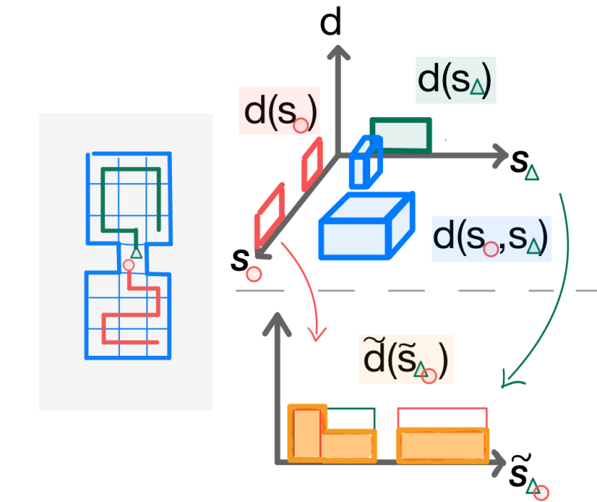
Figure 1: The interaction on the left induces different (empirical) distributions: marginal distributions for agent 1 and agent 2 over their respective states; a joint distribution over the product space; a mixture distribution over a common space, defined as the average. The mixture distribution is usually less sparse.

Similarly to what happens for the joint distribution, one can define the empirical distribution induced by $K$ episodes as $\tilde{d}_{K}(\tilde{s})=\frac{1}{|\mathcal{N}|}\sum_{i\in[\mathcal{N}]}d_{K,i}(\tilde{s})$ and $\tilde{d}^{\pi}=\operatorname*{\mathbb{E}}_{\tilde{d}_{K}\sim p^{\pi}_{K}}[\tilde{d}_{K}]$. The mixture distribution allows for the definition of the Mixture objectives, in their infinite and finite trials formulations respectively:

$$\max_{\pi=(\pi^{i}\in\Pi^{i})_{i\in[\mathcal{N}]}}\ \Big{\{}\tilde{\zeta}_{\infty}(\pi) :=\mathcal{F}(\tilde{d}^{\pi})\Big{\}}$$ (5)

$$\max_{\pi=(\pi^{i}\in\Pi^{i})_{i\in[\mathcal{N}]}}\ \Big{\{}\tilde{\zeta}_{K}(\pi) :=\operatorname*{\mathbb{E}}_{\tilde{d}_{K}\sim p^{\pi}_{K}}\mathcal{F}(\tilde{d}_{K})\Big{\}}$$ (6)

By employing this kind of objectives in the task-agnostic exploration, i.e. by setting $\mathcal{F}(\cdot):=H(\cdot)$, two are the possible scenarios of optimal behaviors. In the first scenario, each agent tries to cover her state space as uniformly as possible, without taking into account the presence of others. In this sense, the mixture objectives enforce a behavior similar to the disjoint ones. The second scenario is more interesting and it has been referred to in Kolchinsky & Tracey (2017) for general distributions as the clustered scenario: agents will form a grouping such that marginal distributions in the same group are approximately the same, while distributions assigned to different groups will be very different from one another, potentially with a disjoint support. In other words, agents will try to cover different sub-portions of the state space in groups, so that, on average, all the state space will be covered uniformly. This second scenario is of particular interest for task-agnostic exploration, as it is the only one among the one presented that explicitly enforces policies inducing diverse state distributions among the agents.

Remarks.

Mixture objectives in task-agnostic exploration require estimating the entropy of mixture state-distributions, which might remain challenging in high-dimensional scenarios. Fortunately, the problem of efficiently estimating the entropy for general mixture distributions has been previously investigated in Kolchinsky & Tracey (2017) and extended to RL with mixture policies by Baram et al. (2021). The same ideas might be applied to the case of interest.

4 A Formal Characterization of Multi-Agent Task-Agnostic Exploration

In the previous section, we described how different objectives enforce different behaviors for task-agnostic explorative policies. In this section, we address the second research question:

(ii) Are different formulations related in some way and when crucial differences emerge?

First of all, we show that if we look at task-agnostic exploration tasks, i.e. the ones defined by setting the functional $\mathcal{F}(\cdot):=H(\cdot)$, all the objectives in infinite-trials formulation can be elegantly linked one to the other though the following result:

Lemma 4.1 (Entropy Mismatch).

For every Convex Markov Game $\mathcal{M}_{H}$ equipped with an entropy functional, for a fixed (joint) policy $\pi=(\pi^{i})_{i\in\mathcal{N}}$ the infinite-trials objectives are ordered according to:

$$\frac{H(d^{\pi})}{|\mathcal{N}|} \leq\frac{1}{|\mathcal{N}|}\sum_{i\in[\mathcal{N}]}H(d_{i}^{\pi})\leq H(\tilde{d}^{\pi})$$

$$H(\tilde{d}^{\pi})\leq\sup_{i\in[\mathcal{N}]} H(d_{i}^{\pi})+\log(|\mathcal{N}|)\leq H(d^{\pi})+\log(|\mathcal{N}|)$$

The full derivation of these bounds is reported in Appendix A. This set of bounds prescribe that the difference in performances over infinite-trials objective for the same policy can be generally bounded as a function of the number of agents. In particular, disjoint objectives generally provides poor approximations of the joint objective from the point of view of the single-agent, while the mixture objective is guaranteed to be a rather good lower bound to the joint entropy as well, since its over-estimation scales logarithmically with the number of agents.

It is still an open question how hard it is to actually optimize for these objectives. Now, while CMGs are a novel interaction framework, whose general properties are far from being well-understood, they surely enjoy some nice properties. In particular, as commonly done in Potential Markov Games (Leonardos et al., 2021), it is possible to exploit the fact that performing Policy Gradient (PG, Sutton et al., 1999; Peters & Schaal, 2008) independently among the agents is equivalent to running PG jointly, when this is done over the same common objective (Appendix A.1, Lemma A.5). This allows us to provide a rather positive answer, here stated informally and extensively discussed in Appendix A.1 :

Fact 4.1 ((Informal) Sufficiency of Independent Policy Gradient).

Under proper assumptions, for every CMG $\mathcal{M}_{\mathcal{F}}$, independent Policy Gradient over infinite trials non-disjoint objectives via centralized policies of the form $\pi=(\pi^{i}\in\Delta_{\mathcal{S}}^{\mathcal{A}^{i}})_{i\in[\mathcal{N}]}$ converges fast.

This result suggests that PG should be generally enough for the infinite-trials optimization, and thus, from a certain point of view, these problems might not be of so much interest. However, convex MDP theory has outlined that optimizing for infinite-trials objectives might actually lead to extremely poor performances as soon as the policies are deployed over just a handful of trials, i.e. in almost any practical scenario (Mutti et al., 2023a). We show that this property transfers almost seamlessly to CMGs as well, with interesting additional take-outs:

Theorem 4.2 (Objectives Mismatch in CMGs).

For every CMG $\mathcal{M}_{\mathcal{F}}$ equipped with a $L$-Lipschitz function $\mathcal{F}$, let $K\in\mathbb{N}^{+}$ be a number of evaluation episodes/trials, and let $\delta\in(0,1]$ be a confidence level, then for any (joint) policy $\pi=(\pi^{i}\in\Pi^{i})_{i\in[\mathcal{N}]}$, it holds that

$$|\zeta_{K}(\pi)-\zeta_{\infty}(\pi)|\leq LT\sqrt{\frac{2|\mathcal{S}|\log(2T/\delta)}{K}},$$

$$|\zeta^{i}_{K}(\pi)-\zeta^{i}_{\infty}(\pi)|\leq LT\sqrt{\frac{2|\tilde{\mathcal{S}}|\log(2T/\delta)}{K}},$$

$$|\tilde{\zeta}_{K}(\pi)-\tilde{\zeta}_{\infty}(\pi)|\leq LT\sqrt{\frac{2|\tilde{\mathcal{S}}|\log(2T/\delta)}{|\mathcal{N}|K}}.$$

In general, this set of bounds confirms that infinite and finite trials objectives might be extremely different, and thus optimizing the infinite-trials objective might lead to unpredictable performance at deployment, whenever this is done over a handful of trials. This property is inherently linked to the convex nature of convex MDPs, and Mutti et al. (2023a) introduces it to highlight that the concentration properties of empirical state-distributions (Weissman et al., 2003) allow for a nice dependency on the number of trials in controlling the mismatch. In multi-agent settings, the result portraits a more nuanced scene:
(i) The mismatch still scales with the cardinality of the support of the state distribution, yet, for joint objectives, this quantity scales very poorly in the number of agents. Thus, even though optimizing infinite-trials joint objectives might be rather easy in theory as Fact 4.1 suggests, it might result in poor performances in practice. On the other hand, the quantity is independent of the number of agents for disjoint and mixture objectives.
(ii) Looking at mixture objectives, the mismatch scales sub-linearly with the number of agents $\mathcal{N}$. Thus, in some sense, the number of agents has the same role as the number of trials: the more the agents the less the deployment mismatch, and at the limit, with $\mathcal{N}\rightarrow\infty$, the mismatch vanishes completely. In other words, this result portraits a striking difference with respect to joint objectives: when facing task-agnostic exploration over mixtures, a reasonably high number of agents compared to the size of the state-space actually helps, and simple policy gradient over mixture objectives might be enough.

Remarks.

One should notice that the results of Fact 4.1 are valid only for specific classes of policies, namely centralized policies of the form $\pi=(\pi^{i}\in\Delta_{\mathcal{S}}^{\mathcal{A}^{i}})_{i\in[\mathcal{N}]}$. Up to our knowledge, no guarantees are known for decentralized policies even in linear MGs. Interestingly though, the finite-trials formulation do offer additional insights on the behavior of optimal decentralized policies, a striking difference with respect to both the infinite-trial objectives and the linear MG interaction model in general. The interested reader can learn more about this in Appendix A.2.

5 Trust Region for Exploration in Practice

As stated before, a core drive of this work is addressing multi-agent task-agnostic exploration in practical scenarios. Yet, these cases are also the ones in which performing PG of infinite-trials objectives provide poor performance guarantees at deployment. In other words, here we address the third research question, that is:

(iii) How can we explicitly address multi-agent task-agnostic exploration in practical scenarios?

To do so, our attention will focus on the finite trials objectives explicitly, more specifically on the single-trial case with $K=1$. Remarkably, it is possible to directly optimize the single-trial objective in multi-agent cases with decentralized algorithms: we introduce Trust Region Pure Exploration (TRPE), the first decentralized algorithm that explicitly addresses single-trial objectives in CMGs, with task-agnostic exploration as a special case. TRPE takes inspiration from trust-region based methods as TRPO (Schulman et al., 2017), as they recently enjoyed an ubiquitous success and interest for their surprising effectiveness in multi-agent problems (Yu et al., 2022).

In fact, trust-region analysis nicely align with the properties of finite-trials formulations and allow for an elegant extension to CMGs through the following.

Definition 5.1 (Surrogate Function over a Single Trial).

For every CMG $\mathcal{M}_{\mathcal{F}}$ equipped with a $L$-Lipschitz function $\mathcal{F}$, let $d_{1}$ be a general single-trial distribution $d_{1}=\{d_{1},d_{1,i},\tilde{d}_{1}\}$, then for any per-agent deviation over policies $\pi=(\pi^{i},\pi^{-i})$, $\tilde{\pi}=(\tilde{\pi}^{i},\pi^{-i})$, it is possible to define a per-agent Surrogate Function $\mathcal{L}^{i}(\tilde{\pi}/\pi)$ of the form

$$\mathcal{L}^{i}(\tilde{\pi}/\pi)=\operatorname*{\mathbb{E}}_{d_{1}\sim p^{\pi}_{1}}\rho^{i}_{\tilde{\pi}/\pi}\mathcal{F}(d_{1}),\vskip-5.69046pt$$

where $\rho^{i}$ is the per-agent importance-weight coefficient $\rho^{i}_{\tilde{\pi}/\pi}=p^{\tilde{\pi}}_{1}/p^{\pi}_{1}=\prod_{t\in[T]}\frac{\tilde{\pi}^{i}(\mathbf{a}^{i}[t]|\mathbf{s}^{i}[t])}{\pi^{i}(\mathbf{a}^{i}[t]|\mathbf{s}^{i}[t])}$, such that for $\zeta_{1}\in\{\zeta_{1}^{\infty},\zeta_{1}^{i},\tilde{\zeta}_{1}\}$.

Algorithm 1 Trust Region Pure Exploration (TRPE)

 Input: exploration horizon $T$, number of trajectories $N$, trust-region threshold $\delta$, learning rate $\eta$.

 initialize $\bm{\theta}=(\theta^{i})_{i\in[\mathcal{N}]}$

 for epoch = $1,2,\ldots,$ until convergence do

  Collect $N$ trajectories with $\pi_{\bm{\theta}}=(\pi^{i}_{\theta^{i}})_{i\in[\mathcal{N}]}$.

  for agent $i=1,2,\ldots,$ concurrently do

   Construct datasets $\mathcal{D}^{i}=\{(\mathbf{s}^{i}_{n},\mathbf{a}^{i}_{n}),\zeta_{1}^{n}\}_{n\in[N]}$

   $\theta^{i}\leftarrow\emph{IS-Optimizer}(\mathcal{D}^{i},\theta^{i})$

  end for

 end for

 Output: task-agnostic exploration (joint) policy $\pi_{\bm{\theta}}=(\pi^{i}_{\theta^{i}})_{i\in[\mathcal{N}]}$

 

IS-Optimizer

 

 Input: Dataset $\mathcal{D}^{i}$, sampling parameter $\theta^{i}$.

 Initialize $h=0$ and $\theta^{i}_{h}=\theta^{i}$

 while  $D_{\mathrm{KL}}(\pi^{i}_{\theta^{i}_{h}}\|\pi^{i}_{\theta^{i}_{0}})\leq\delta$ do

  Compute $\hat{\mathcal{L}}^{i}(\theta^{i}_{h}/\theta^{i}_{0})$ via IS

  Perform Gradient step $\theta^{i}_{h+1}=\theta^{i}_{h}+\eta\nabla_{\theta^{i}_{h}}\hat{\mathcal{L}}^{i}(\theta^{i}_{h}/\theta^{i}_{0})$

  $h\leftarrow h+1$

 end while

 Output: parameters $\bm{\theta}_{h}$

From this definition, it follows that the trust-region algorithmic blueprint of Schulman et al. (2017) can be directly applied to single-trial formulations, with per-agent policies within a parametric space of stochastic differentiable policies $\Theta=\{\pi^{i}_{\theta^{i}}:\theta^{i}\in\Theta^{i}\subseteq\mathbb{R}^{q}\}$. In practice, kl-divergence is employed for greater scalability provided a trust-region threshold $\delta$, we address the following optimization problem for each agent:

$$\max_{\tilde{\theta}^{i}\in\Theta^{i}}\mathcal{L}^{i}(\tilde{\theta}^{i}/\theta^{i}),$$

$$\text{s.t. }D_{\mathrm{KL}}(\pi^{i}_{\tilde{\theta}^{i}}\|\pi^{i}_{\theta^{i}})\leq\delta\vskip-8.5359pt$$

where we simplified the notation by letting $\mathcal{L}^{i}(\tilde{\theta}^{i}/\theta^{i}):=\mathcal{L}^{i}(\pi^{i}_{\tilde{\theta}^{i}},\pi^{-i}_{\theta^{-i}}/\pi_{\theta})$.

(a) Joint Entropy.

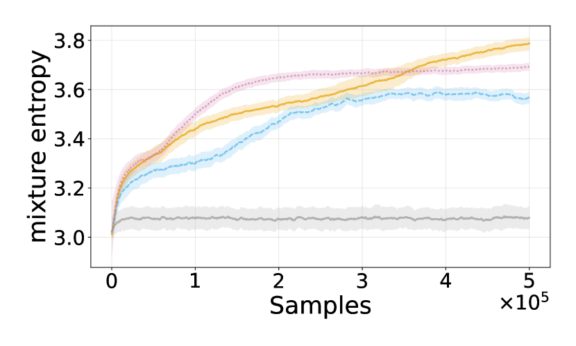
(b) Mixture Entropy.

Figure 2: Single-trial Joint and Mixture Entropy induced by mixture, joint or disjoint objective optimization along a $T=50$ horizon. (Right) State Distributions of two agents induced by different learned policies. We report the average and 95% c.i. over 4 runs.

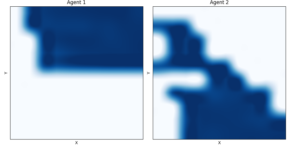
(c) Mixture

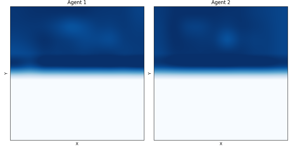
(d) Joint

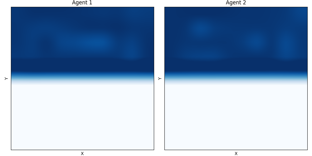
(e) Disjoint

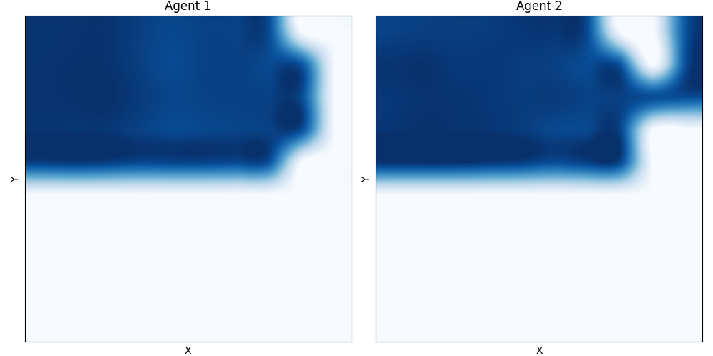
(f) Uniform

The main idea then follows from noticing that the surrogate function in Eq. (5.1) consists of an Importance Sampling (IS) estimator (Owen, 2013), and it is then possible to optimize it in a fully decentralized and off-policy manner, similarly to what was done in Metelli et al. (2020) for MDPs and in Mutti & Restelli (2020) for convex MDPs. More specifically, given a pre-specified objective of interest $\zeta_{1}\in\{\zeta_{1}^{\infty},\zeta_{1}^{i},\tilde{\zeta}_{1}\}$, agents sample $N$ trajectories $\{(\mathbf{s}_{n},\mathbf{a}_{n})\}_{n\in[N]}$ from the environment by following a (joint) policy with parameters $\bm{\theta}_{0}=(\theta^{i}_{0},\theta^{-i}_{0})$. They then compute the values of the objective for each trajectory, building separate datasets $\mathcal{D}^{i}=\{(\mathbf{s}^{i}_{n},\mathbf{a}^{i}_{n}),\zeta_{1}^{n}\}_{n\in[N]}$. Each agent uses her dataset to compute the Monte-Carlo approximation of the Surrogate Function, namely:

$$\vskip-5.69046pt\hat{\mathcal{L}}^{i}(\theta^{i}_{h}/\theta^{i}_{0})=\frac{1}{N}\sum_{n\in[N]}\rho^{i,n}_{\theta^{i}_{h}/\theta^{i}_{0}}\zeta^{n}_{1},\vskip-0.28436pt$$

where $\rho^{i,n}_{\theta^{i}_{h}/\theta^{i}_{0}}=\prod_{t\in[T]}\pi^{i}_{\theta^{i}_{h}}(\mathbf{a}^{i}_{n}[t]|\mathbf{s}^{i}_{n}[t])/\pi^{i}_{\theta^{i}_{0}}(\mathbf{a}^{i}_{n}[t]|\mathbf{s}^{i}_{n}[t])$ and $\zeta^{n}_{1}$ is the plug-in estimator of the entropy based on the empirical measure $d_{1}$ (Paninski, 2003). Finally, at each off-policy iteration $h$, each agent updates its parameter via gradient ascent $\theta^{i}_{h+1}\leftarrow\theta^{i}_{h}+\eta\nabla_{\theta^{i}_{h}}\hat{\mathcal{L}}^{i}(\theta^{i}_{h}/\theta^{i}_{0})$ until the trust-region boundary is reached, i.e., when it holds $D_{\mathrm{KL}}(\pi^{i}_{\tilde{\theta}^{i}}\|\pi^{i}_{\theta^{i}})>\delta.$ The psudo-code of TRPE is reported in Algorithm 1.

Remark.

One should note that TRPE is a multi-agent decentralized algorithm and it explicitly addresses task-agnostic exploration objectives, however the algorithmic blueprint is of independent interest since it is both able to address any convex functional $\mathcal{F}(\cdot)$, and it is valid in the single agent case as well.

6 Proof of Concept Experiments

In this section, we provide some empirical validations of the findings discussed so far. Especially, we aim to answer the following questions: (a) Is Algorithm 1 actually capable of optimizing finite-trials objectives? (b) Do different objectives enforce different behaviors, as expected from Section 3? (c) Does the clustering behavior of mixture objectives play a crucial role? If yes, when and why?
Throughout the experiments, we will compare the result of optimizing finite-trial objectives, either joint, disjoint, mixture ones, through Algorithm 1 via fully decentralized policies. The experiments will be performed with different values of the exploration horizon $T$, so as to test their capabilities in different exploration efficiency regimes. The full implementation details are reported in Appendix B.

Experimental Domains.

The experiments were performed on two domains. The first is a notoriously difficult multi-agent exploration task called secret room (MPE, Liu et al., 2021b), referred to as Env. (i). In such task, two agents are required to reach a target while navigating over two rooms divided by a door. In order to keep the door open, at least one agent have to remain on a switch. Two switches are located at the corners of the two rooms. The hardness of the task then comes from the need of coordinated exploration, where one agent allows for the exploration of the other. The second is a simpler exploration task yet over a high dimensional state-space, namely a 2-agent instantiation of Reacher (MaMuJoCo, Peng et al., 2021), referred to as Env. (ii). Each agent corresponds to one joint and equipped with decentralized policies conditioned on her own states. In order to allow for the use of plug-in estimator of the entropy (Paninski, 2003), each state dimension was discretized over 10 bins.

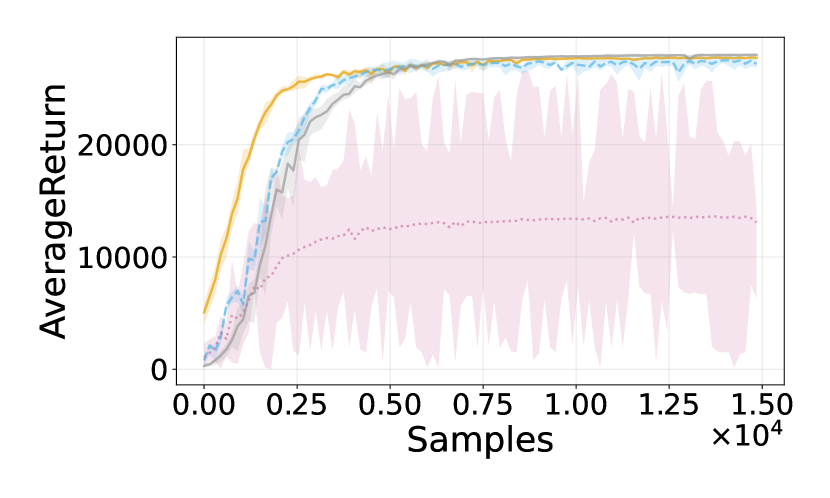
(a) MA-TRPO with TRPE Pre-Training (Env. (i), $T=150$).

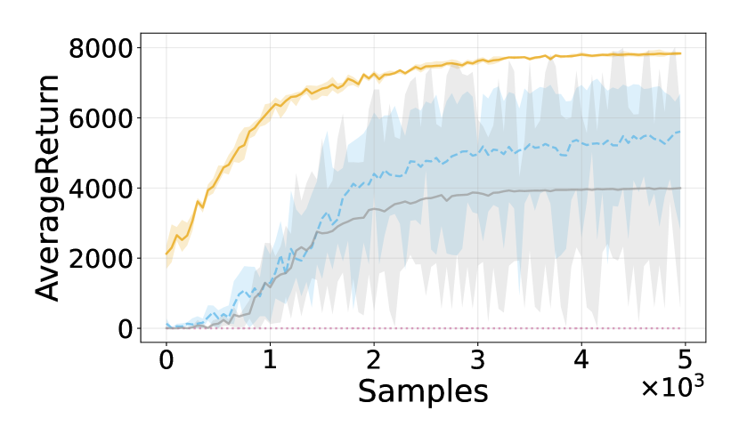
(b) MA-TRPO with TRPE Pre-Training (Env. (i), $T=50$).

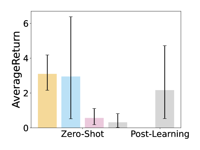
(c) MA-TRPO with TRPE Pre-Training (Env. (ii), $T=100$).

Figure 3: Effect of pre-training in sparse-reward settings.(left) Policies initialized with either Uniform or TRPE pre-trained policies over 4 runs over a worst-case goal. (rigth) Policies initialized with either Zero-Mean or TRPE pre-trained policies over 4 runs over 3 possible goal state. We report the average and 95% c.i.

Task-Agnostic Exploration.

Algorithm 1 was first tested in her ability to address task-agnostic exploration per se. This was done by considering the well-know hard-exploration task of Env. (i). The results are reported in Figure 2(b) for a short exploration horizon $(T=50)$. Interestingly, at this efficiency regime, when looking at the joint entropy in Figure 2(a), joint and disjoint objectives perform rather well compared to mixture ones in terms of induced joint entropy, while they fail to address mixture entropy explicitly, as seen in Figure 2(b). On the other hand mixture-based objectives result in optimizing both mixture and joint entropy effectively, as one would expect by the bounds in Th. 4.1. By looking at the actual state visitation induced by the trained policies, the difference between the objectives is apparent. While optimizing joint objectives, agents exploit the high-dimensionality of the joint space to induce highly entropic distributions even without exploring the space uniformly via coordination (Fig. 2(d)); the same outcome happens in disjoint objectives, with which agents focus on over-optimizing over a restricted space loosing any incentive for coordinated exploration (Fig.2(e)). On the other hand, mixture objectives enforce a clustering behavior (Fig.2(e)) and result in a better efficient exploration.

Policy Pre-Training via Task-Agnostic Exploration.

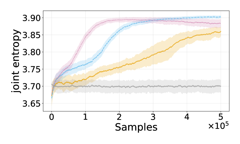
(a) TRPE Joint Entropy (Env. (i), $T=50$).

(b) TRPE Mixture Entropy (Env. (i), $T=50$).

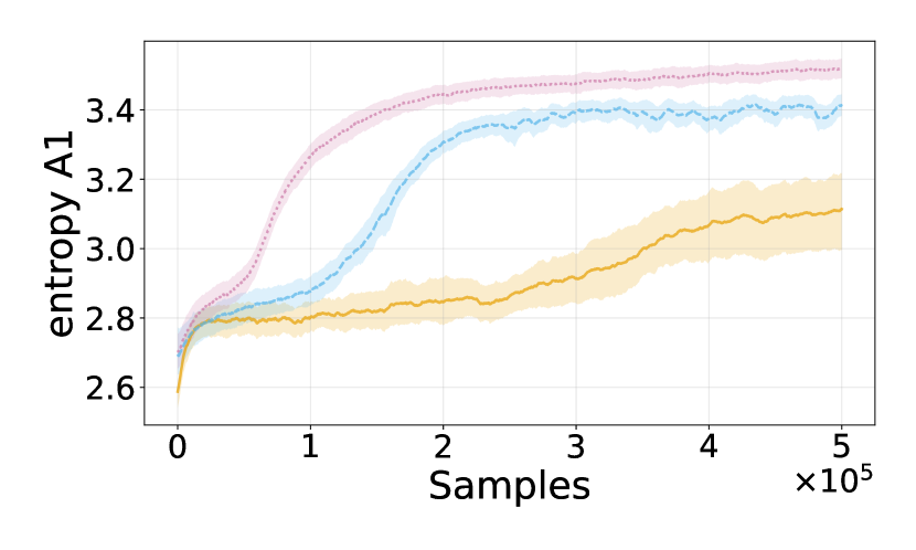
(c) TRPE Entropy Agent 1 (Env. (i), $T=50$).

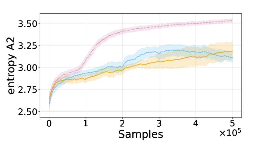
(d) TRPE Entropy Agent 2 (Env. (i), $T=50$).

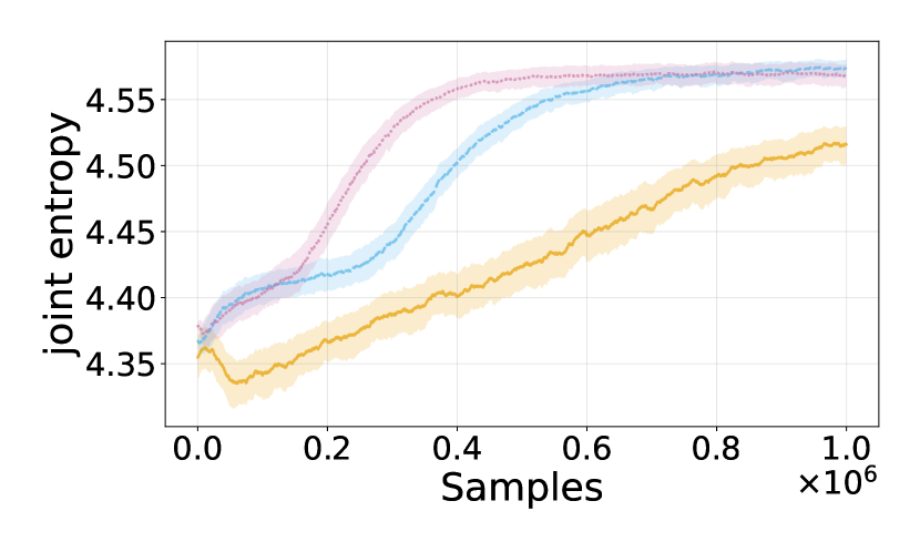
(e) TRPE Joint Entropy (Env. (i), $T=100$).

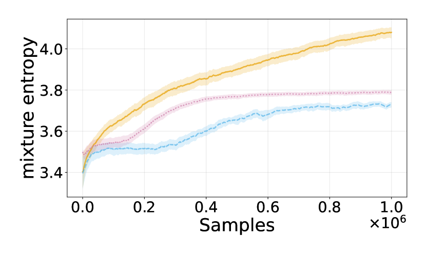
(f) TRPE Mixture Entropy (Env. (i), $T=100$).

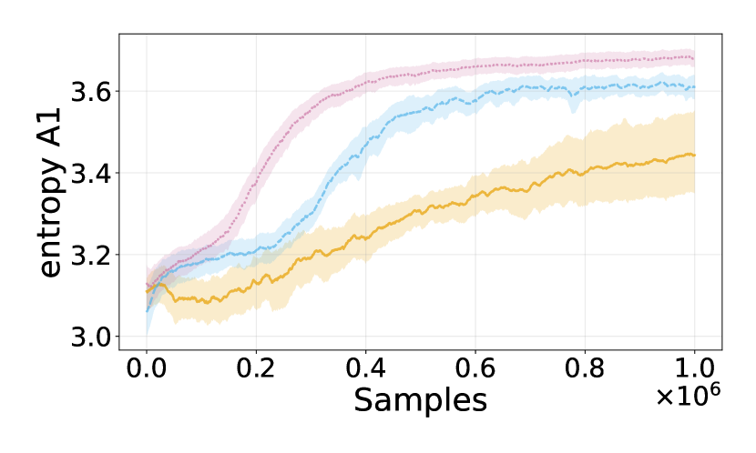
(g) TRPE Entropy Agent 1 (Env. (i), $T=100$).

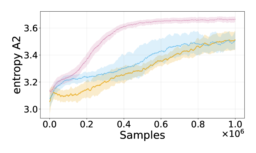
(h) TRPE Entropy Agent 2 (Env. (i), $T=100$).

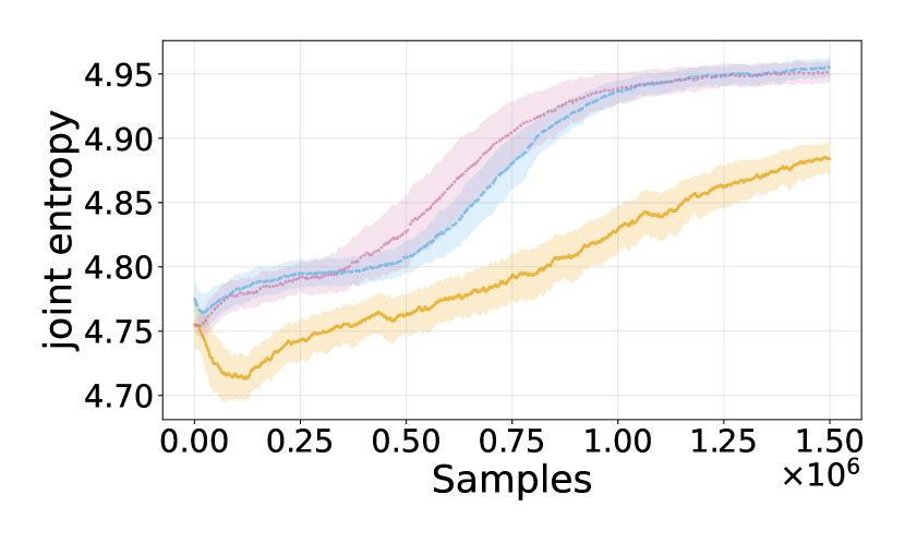
(i) TRPE Joint Entropy (Env. (i), $T=150$).

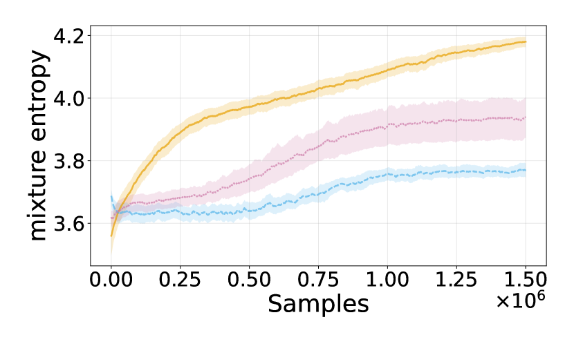
(j) TRPE Mixture Entropy (Env. (i), $T=150$).

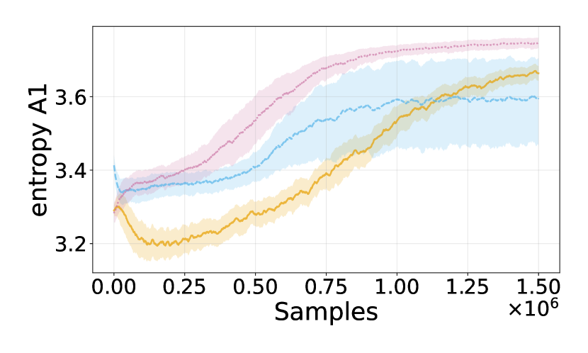
(k) TRPE Entropy Agent 1 (Env. (i), $T=150$).

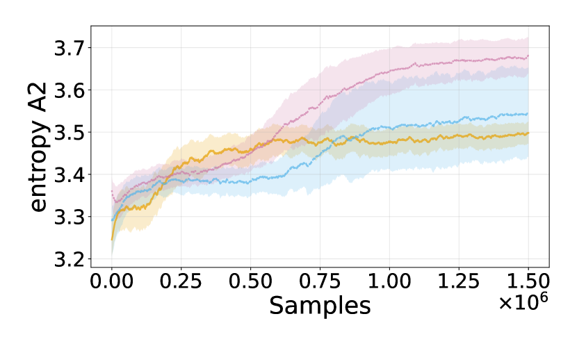
(l) TRPE Entropy Agent 2 (Env. (i), $T=150$).

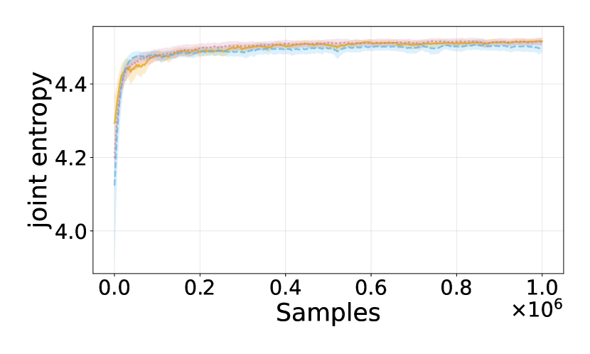
(m) TRPE Joint Entropy (Env. (ii), $T=100$).

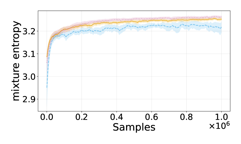
(n) TRPE Mixture Entropy (Env. (ii), $T=100$).

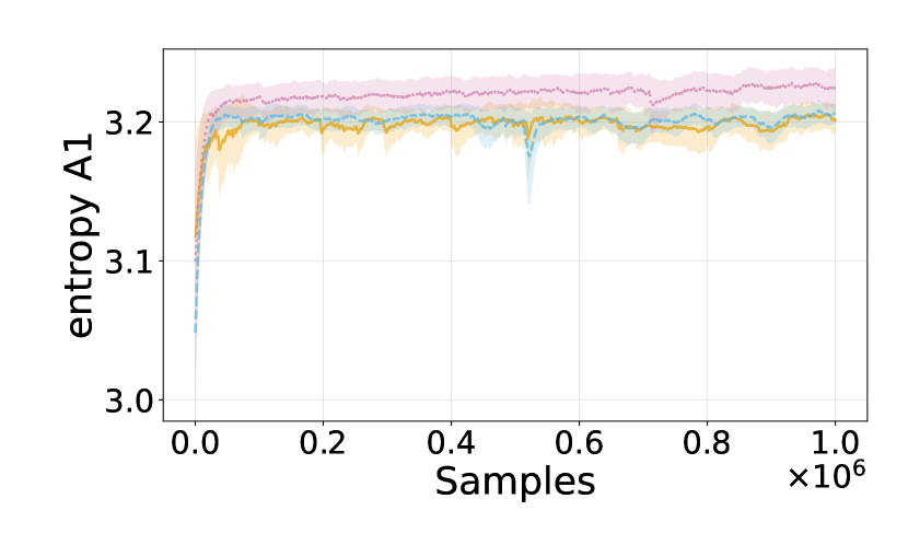
(o) TRPE Entropy Agent 1 (Env. (ii), $T=100$).

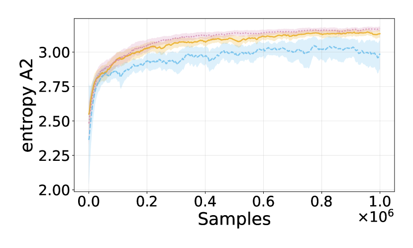
(p) TRPE Entropy Agent 2 (Env. (ii), $T=100$).

Figure 4: Full Visualization of Reported Experiments.

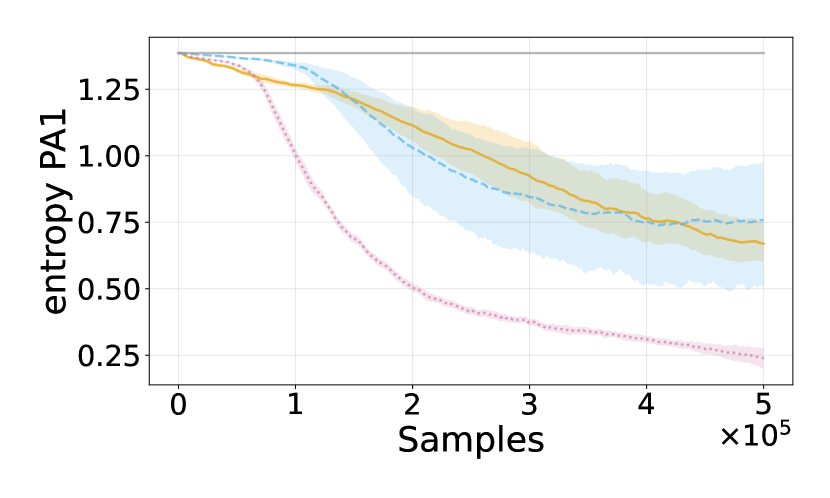
(a) Entropy of Agent 1 Policy in TRPE Training (i), $T=50$).

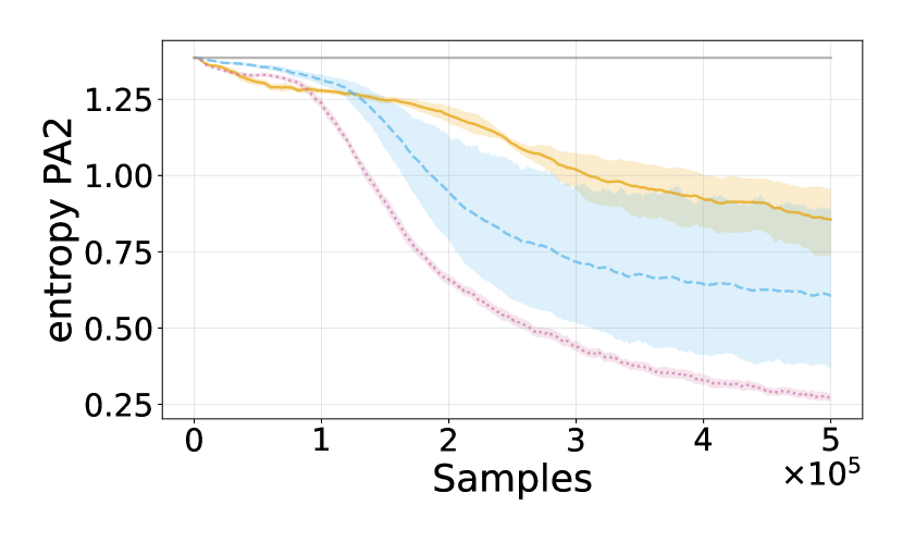
(b) Entropy of Agent 2 Policy in TRPE Training (i), $T=50$).

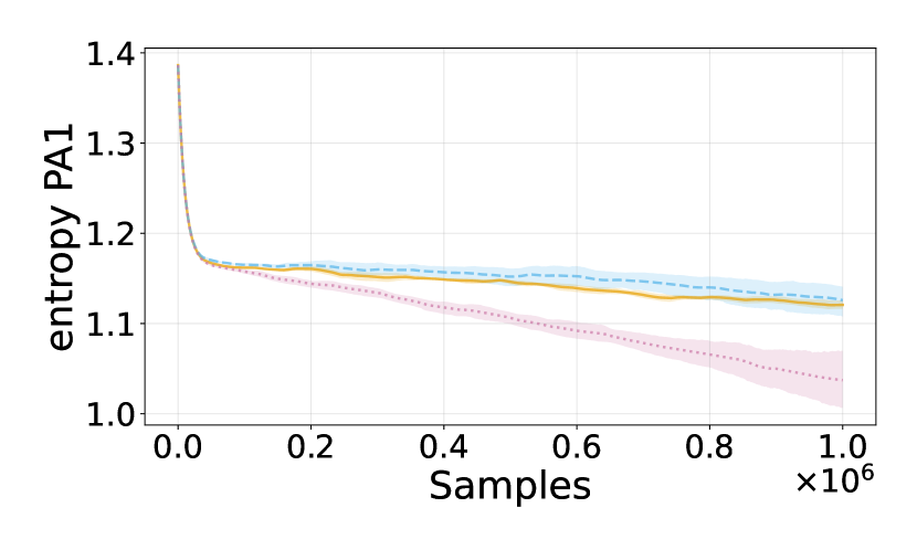
(c) Entropy of Agent 1 Policy in TRPE Training (ii), $T=100$).

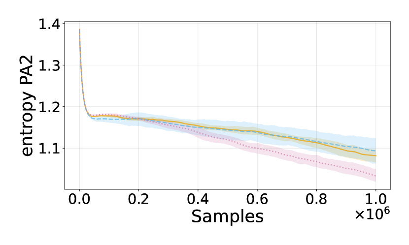
(d) Entropy of Agent 2 Policy in TRPE Training (ii), $T=100$).

Figure 5: Policiy Entropy Insights for TRPO Pretraining in Env (i) and Env (ii). Lower Entropic Policies with Disjoint Objectives might justify the difference in pre-training performance even if the performances in training are similar.

More interestingly, we tested the effect of pre-training policies via different objectives as a way to alleviate the well-known hardness of sparse-reward settings, either throught faster learning or zero-short generalization. In order to do so, we employed a multi-agent counterpart of the TRPO algorithm (Schulman et al., 2017) with different pre-trained policies. First, we investigated the effect on the learning curve in the hard-exploration task of Env. (i) under long horizons ($T=150$), with a worst-case goal set on the the opposite corner of the closed room. Pre-training via mixture objectives still lead to a faster learning compared to initializing the policy with a uniform distribution. On the other hand, joint objective pre-training did not lead to substantial improvements over standard initializations. More interestingly, when extremely short horizons were taken into account ($T=50$) the difference became appalling, as shown in Fig. 3(a): pre-training via mixture-based objectives leaded to faster learning and higher performances, while pre-training via disjoint objectives turned out to be even harmful (Fig. 3(b)). This was motivated by the fact that the disjoint objective overfitted the task over the states reachable without coordinated exploration, resulting in almost deterministic policies, as shown in Fig 5 in Appendix B. Finally, we tested the zero-shot capabilities of policy pre-training on the simpler but high dimensional exploration task of Env. (ii), where the goal was sampled randomly between worst-case positions at the boundaries of the region reachable by the arm. As shown in Fig. 4(p), both joint and mixture were able to guarantee zero-shot performances via pre-training compatible with MA-TRPO after learning over $2$e$4$ samples, while disjoint objectives were not. On the other hand, pre-training with joint objectives showed an extremely high-variance, leading to worst-case performances not better than the ones of random initialization. Mixture objectives on the other hand showed higher stability in guaranteeing compelling zero-shot performance.

Take-Aways.

Overall, the proposed proof of concepts experiments managed to answer to all of the experimental questions: (a) Algorithm 1 is indeed able to explicitly optimize for finite-trial entropic objectives. Additionally, (b) mixture distributions enforce diverse yet coordinated exploration, that helps when high efficiency is required. Joint or disjoint objectives on the other hand may fail to lead to relevant solutions because of under or over optimization. Finally, (c) efficient exploration enforced by mixture distributions was shown to be a crucial factor not only for the sake of task-agnostic exploration per se, but also for the ability of pre-training via task-agnostic exploration to lead to faster and better training and even zero-shot generalization.

7 Related Works

Below, we summarize the most relevant work investigating multi-agent exploration and task-agnostic exploration in single-agent scenarios.

Multi-Agent Exploration.

Recently, fostering exploration in order to boost performances in (deep) MARL has gained much attention recently. A large set of works proposed to address it via reward-shaping based on many heuristics: Wang et al. (2019) adds a term maximizing the mutual-information between per-agent interactions; Zhang et al. (2021) proposes to optimize the deviation from (jointly) explored regions while Zhang et al. (2023) proposes to optimize directly the entropy over per-agent observations; more recently, Xu et al. (2024) proposed an heuristic reward-shaping enforcing diversity between different agents, and notices that Wang et al. (2019) fails to address the task it introduced. Up to our knowledge, this work is the first in covering both the theoretical properties of multi-agent (task-agnostic) exploration and the optimization of single-trial objectives. Finally, we notice that a that a similar notion of Convex Markov Games was introduced in a concurrent and preliminary work (Gemp et al., 2025), together with some results on existence of equilibria.

Task-Agnostic Exploration and Policy Optimization.

Entropy maximization in MDPs was first introduced in Hazan et al. (2019) and then investigated extensively in a blossoming of different works, addressing the entropy over (trajectories of) states or even observations (to name a few Jin et al., 2020; Golowich et al., 2022; Tiapkin et al., 2023; Zamboni et al., 2024; Savas et al., 2022). Finally, the use of trust-region schemes (Schulman et al., 2017) is ubiquitous in RL. We considered an importance-sampling policy gradient estimator inspired by the work of Metelli et al. (2020). It is yet possible to use other forms of IS estimators, as non-parametric k-NN estimators proposed in Mutti & Restelli (2020).

8 Conclusions and Perspectives

In this paper, we extend the state entropy maximization problem to Markov Games via a novel framework called Convex Markov Games. First of all, we show that the task can be defined in several different ways: one can look at the joint distribution among all the agents, the marginals which are agent-specific, or the mixture which is a tradeoff of the two. Thus, we link these three options via performance bounds and we show that while the first might enjoy nice theoretical guarantees, the others are more promising at working in practice, the latter in particular. Then, we design a practical trust-region algorithm addressing more practical scenarios and we use it to confirm in a set of experiments the expected superiority of mixture objectives, due to its ability to enforce efficient but coordinated exploration over short horizons. Future works can build over our results in many directions, which include pushing forward the known theoretical properties of Convex Markov Games, developing scalable algorithms for continuous domains and investigating more policy classes with succinct representations of the history beyond the one we considered in the experiments. We believe that our work can be a crucial step in the direction of extending state entropy maximization in a principled way to yet more practical settings, in which many agents interact over the same environment.

Impact Statement

This paper presents work whose goal is to advance the field of Machine Learning. There are many potential societal consequences of our work, none which we feel must be specifically highlighted here.

Appendix A Proofs of the Main Theoretical Results

In this Section, we report the full proofing steps of the Theorems and Lemmas in the main paper.

See 4.1

Proof.

The bounds follow directly from simple yet fundamental relationships between entropies of joint, marginal and mixture distributions which can be found in Paninski (2003); Kolchinsky & Tracey (2017), in particular:

$$\frac{1}{|\mathcal{N}|}H(d^{\pi})\leq\frac{1}{|\mathcal{N}|}\sum_{i\in[\mathcal{N}]}H(d_{i}^{\pi})\overset{\text{(a)}}{\leq}H(\tilde{d}^{\pi})\overset{\text{(b)}}{\leq}\frac{1}{|\mathcal{N}|}\sum_{i\in[\mathcal{N}]}H(d_{i}^{\pi})+\log(|\mathcal{N}|)\overset{\text{(c)}}{\leq}\sup_{i\in[\mathcal{N}]}H(d_{i}^{\pi})+\log(|\mathcal{N}|)\leq H(d^{\pi})+\log(|\mathcal{N}|)$$

where step (a) and (b) use the fact that $\tilde{d}^{\pi}(s):=\frac{1}{|\mathcal{N}|}\sum_{i\in[\mathcal{N}]}d^{\pi}_{i}(s)$ is a uniform mixture over the agents, whose distribution over the weights has entropy $\log(|\mathcal{N}|)$, so as we can apply the bounds from Kolchinsky & Tracey (2017). Step (c) uses the fact that $H(d^{\pi})=\sum_{i\in[\mathcal{N}]}H(d^{\pi}_{i}|d^{\pi}_{<i})$, then taking the supremum as first $i$ it follows that $\sup_{i\in[\mathcal{N}]}H(d_{i}^{\pi})=H(d^{\pi})-\sum_{j\in[\mathcal{N}]>i}H(d^{\pi}_{j}|d^{\pi}_{<j},d^{\pi}_{i})\leq H(d^{\pi})$ due to non-negativity of entropy. ∎

See 4.2

Proof.

For the general proof structure, we adapt the steps of Mutti et al. (2023b) for Convex MDPs to the different objectives possible in CMGs. Let us start by considering joint objectives, then:

$$\big{|}\zeta_{K}(\pi)-\zeta_{\infty}(\pi)\big{|} =\Big{|}\operatorname*{\mathbb{E}}_{d_{K}\sim p^{\pi}_{K}}\left[\mathcal{F}(d_{K})\right]-\mathcal{F}(d^{\pi})\Big{|}\leq\operatorname*{\mathbb{E}}_{d_{K}\sim p^{\pi}_{K}}\left[\left|\mathcal{F}(d_{K})-\mathcal{F}(d^{\pi})\right|\right]$$

$$\overset{\text{(a)}}{\leq}\operatorname*{\mathbb{E}}_{d_{K}\sim p^{\pi}_{K}}\left[L\left\|d_{K}-d^{\pi}\right\|_{1}\right]\leq L\operatorname*{\mathbb{E}}_{d_{K}\sim p^{\pi}_{K}}\left[\left\|d_{K}-d^{\pi}\right\|_{1}\right]$$

$$\overset{\text{(b)}}{\leq}L\operatorname*{\mathbb{E}}_{d_{K}\sim p^{\pi}_{K}}\left[\max_{t\in[T]}\left\|d_{K,t}-d^{\pi}_{t}\right\|_{1}\right],$$

where in step (a) we apply the Lipschitz assumption on $\mathcal{F}$ to write and in step (b) we apply a maximization over the episode’s step by noting that $d_{K}=\frac{1}{T}\sum_{t\in[T]}d_{K,t}$ and $d^{\pi}=\frac{1}{T}\sum_{t\in[T]}d^{\pi}_{t}$. We then apply bounds in high probability

$$Pr\Big{(}\max_{t\in[T]}\left\|d_{K,t}-d^{\pi}_{t}\right\|_{1}\geq\epsilon\Big{)} \leq Pr\Big{(}\bigcup_{t}\left\|d_{K,t}-d^{\pi}_{t}\right\|_{1}\geq\epsilon\Big{)}$$

$$\overset{\text{(c)}}{\leq}\sum_{t}Pr\Big{(}\left\|d_{K,t}-d^{\pi}_{t}\right\|_{1}\geq\epsilon\Big{)}$$

$$\leq T\ Pr\Big{(}\left\|d_{K,t}-d^{\pi}_{t}\right\|_{1}\geq\epsilon\Big{)},$$

with $\epsilon>0$ and in step (c) we applied a union bound. We then consider standard concentration inequalities for empirical distributions (Weissman et al., 2003) so to obtain the final bound

$$Pr\Bigg{(}\left\|d_{K,t}-d^{\pi}_{t}\right\|_{1}\geq\sqrt{\frac{2|\mathcal{S}|\log(2/\delta^{\prime})}{K}}\ \Bigg{)}\leq\delta^{\prime}.$$ (7)

By setting $\delta^{\prime}=\delta/T$, and then plugging the empirical concentration inequality, we have that with probability at least $1-\delta$

$$\big{|}\zeta_{K}(\pi)-\zeta_{\infty}(\pi)\big{|}\leq LT\sqrt{\frac{2|\mathcal{S}|\log(2T/\delta)}{K}},$$

which concludes the proof for joint objectives.

The proof for disjoint objectives follows the same rational by bounding each per-agent term separately and after noticing that due to Assumption 3.1, the resulting bounds get simplified in the overall averaging. As for mixture objectives, the only core difference is after step (b), where $\tilde{d}_{K}$ takes the place of $d_{K}$ and $\tilde{d^{\pi}}$ of $d^{\pi}$. The remaining steps follow the same logic, out of noticing that the empirical distribution with respect to $\tilde{d^{\pi}}$ is taken with respect $|\mathcal{N}|K$ samples in total. Both the two bounds then take into account that the support of the empirical distributions have size $|\tilde{\mathcal{S}}|$ and not $|\mathcal{S}|$. ∎

A.1 Policy Gradient in CMGs with Infinite-Trials.

In this Section, we analyze policy search for the infinite-trials joint problem $\zeta_{\infty}$ of Eq. (1), via projected gradient ascent over parametrized policies, providing in Th. A.6 the formal counterpart of Fact 4.1 in the Main paper. As a side note, all of the following results hold for the (infinite-trials) mixture objective $\tilde{\zeta}_{\infty}$ of Eq. (5). We will consider the class of parametrized policies with parameters $\theta_{i}\in\Theta_{i}\subset\mathbb{R}^{d}$, with the joint policy then defined as $\pi_{\theta},\theta\in\Theta=\times_{i\in[\mathcal{N}]}\Theta_{i}$. Additionally, we will focus on the computational complexity only, by assuming access to the exact gradient. The study of statistical complexity surpasses the scope of the current work. We define the (independent) Policy Gradient Ascent (PGA) update as:

$$\theta^{k+1}_{i}=\operatorname*{arg\,max}_{\theta_{i}\in\Theta_{i}}\zeta_{\infty}(\pi_{\theta^{k}})\!+\!\left\langle\nabla_{\theta_{i}}\zeta_{\infty}(\pi_{\theta^{k}}),\theta_{i}\!-\!\theta^{k}_{i}\right\rangle\!-\!\frac{1}{2\eta}\|\theta_{i}\!-\!\theta_{i}^{k}\|^{2}=\Pi_{\Theta_{i}}\big{\{}\theta^{k}_{i}+\eta\nabla_{\theta_{i}}\zeta_{\infty}(\pi_{\theta^{k}})\big{\}}$$ (8)

where $\Pi_{\Theta_{i}}\{\cdot\}$ denotes Euclidean projection onto $\Theta_{i}$, and equivalence holds by the convexity of $\Theta_{i}$. The classes of policies that allow for this condition to be true will be discussed shortly.

In general the overall proof is built of three main steps, shared with the theory of Potential Markov Games (Leonardos et al., 2021): (i) prove the existence of well behaved stationary points; (ii) prove that performing independent policy gradient is equivalent to perform joint policy gradient; (iii) prove that the (joint) PGA update converges to the stationary points via single-agent like analysis. In order to derive the subsequent convergence proof, we will make the following assumptions:

Assumption A.1.

Define the quantity $\lambda(\theta):=d^{\pi_{\theta}}$, then:
(i). $\lambda(\cdot)$ forms a bijection between $\Theta$ and $\lambda(\Theta)$, where $\Theta$ and $\lambda(\Theta)$ are closed and convex.
(ii). The Jacobian matrix $\nabla_{\theta}\lambda(\theta)$ is Lipschitz continuous in $\Theta$.
(iii). Denote $g(\cdot):=\lambda^{-1}(\cdot)$ as the inverse mapping of $\lambda(\cdot)$. Then there exists $\ell_{\theta}>0$ s.t. $\|g(\lambda)-g(\lambda^{\prime})|\leq\ell_{\theta}\|\lambda-\lambda^{\prime}\|$ for some norm $\|\cdot\|$ and for all $\lambda,\lambda^{\prime}\in\lambda(\Theta)$.

Assumption A.2.

There exists $L>0$ such that the gradient $\nabla_{\theta}\zeta_{\infty}(\pi_{\theta})$ is $L$-Lipschitz.

Assumption A.3.

The agents have access to a gradient oracle $\mathcal{O}(\cdot)$ that returns $\nabla_{\theta_{i}}\zeta_{\infty}(\pi_{\theta})$ for any deployed joint policy $\pi_{\theta}$.

On the Validity of Assumption A.1.

This set of assumptions enforces the objective $\zeta_{\infty}(\pi_{\theta})$ to be well-behaved with respect to $\theta$ even if non-convex in general, and will allow for a rather strong result. Yet, the assumptions are known to be true for directly parametrized policies over the whole support of the distribution $d^{\pi}$ (Zhang et al., 2020), and as a result they implicitly require agents to employ policies conditioned over the full state-space $\mathcal{S}$. Fortunately enough, they also guarantee $\Theta$ to be convex.

Lemma A.4 ((i) Global optimality of stationary policies (Zhang et al., 2020)).

Suppose Assumption A.1 holds, and $\mathcal{F}$ is a concave, and continuous function defined in an open neighborhood containing $\lambda(\Theta)$. Let $\theta^{*}$ be a first-order stationary point of problem (1), i.e.,

$$\exists u^{*}\in\hat{\partial}(\mathcal{F}\circ\lambda)(\theta^{*}),\quad\text{s.t.}\quad\langle u^{*},\theta-\theta^{*}\rangle\leq 0\qquad\mbox{for}\qquad\forall\theta\in\Theta.$$ (9)

Then $\theta^{*}$ is a globally optimal solution of problem (1).

This result characterizes the optimality of stationary points for Eq. (1). Furthermore, we know from Leonardos et al. (2021) that stationary points of the objective are Nash Equilibria.

Lemma A.5 ((ii) Projection Operator (Leonardos et al., 2021)).

Let $\theta:=(\theta_{1},...,\theta_{\mathcal{N}})$ be the parameter profile for all agents and use the update of Eq. (8) over a non-disjoint infinite-trials objective. Then, it holds that

$$\Pi_{\Theta}\big{\{}\theta^{k}+\eta\nabla_{\theta}\zeta_{\infty}(\pi_{\theta^{k}})\big{\}}=\Big{(}\Pi_{\Theta_{i}}\big{\{}\theta^{k}_{i}+\eta\nabla_{\theta_{i}}\zeta_{\infty}(\pi_{\theta^{k}})\big{\}}\Big{)}_{i\in[\mathcal{N}]}$$

This result will only be used for the sake of the convergence analysis, since it allows to analyze independent updates as joint updates over a single objective. The following Theorem is the formal counterpart of Fact 4.1 and it is a direct adaptation to the multi-agent case of the single-agent proof by Zhang et al. (2020), by exploiting the previous result.

Theorem A.6 ((iii) Convergence rate of independent PGA to stationary points (Formal Fact 4.1)).

Let Assumptions A.1 and A.2 hold. Denote $D_{\lambda}\!:=\!\max_{\lambda,\lambda^{\prime}\in\lambda(\Theta)}\|\lambda-\lambda^{\prime}\|$ as defined in Assumption A.1(iii). Then the independent policy gradient update (8) with $\eta=1/L$ satisfies for all $k$ with respect to a stationary (joint) policy $\pi_{\theta^{*}}$ the following

$$\zeta_{\infty}(\pi_{\theta^{*}})\!-\!\zeta_{\infty}(\pi_{\theta^{k}})\leq\frac{4L\ell_{\theta}^{2}D_{\lambda}^{2}}{k+1}.$$

Proof.

First, the Lipschitz continuity in Assumption A.2 indicates that

$$\left|\zeta_{\infty}(\lambda(\theta))-\zeta_{\infty}(\lambda(\theta^{k}))-\langle\nabla_{\theta}\zeta_{\infty}(\lambda(\theta^{k})),\theta-\theta^{k}\rangle\right|\leq\frac{L}{2}\|\theta-\theta^{k}\|^{2}.$$

Consequently, for any $\theta\in\Theta$ we have the ascent property:

$$\zeta_{\infty}(\lambda(\theta))\geq\zeta_{\infty}(\lambda(\theta^{k}))+\langle\nabla_{\theta}\zeta_{\infty}(\lambda(\theta^{k})),\theta-\theta^{k}\rangle-\frac{L}{2}\|\theta-\theta^{k}\|^{2}\geq\zeta_{\infty}(\lambda(\theta))-L\|\theta-\theta^{k}\|^{2}.$$ (10)

The optimality condition in the policy update rule (8) coupled with the result of Lemma A.5 allows us to follow the same rational as Zhang et al. (2020). We will report their proof structure after this step for completeness.

$$\zeta_{\infty}(\lambda(\theta^{k+1}))\geq\zeta_{\infty}(\lambda(\theta^{k}))+\langle\nabla_{\theta}\zeta_{\infty}(\lambda(\theta^{k})),\theta^{k+1}-\theta^{k}\rangle-\frac{L}{2}\|\theta^{k+1}-\theta^{k}\|^{2}$$

$$=\max_{\theta\in\Theta}\zeta_{\infty}(\lambda(\theta^{k}))+\langle\nabla_{\theta}\zeta_{\infty}(\lambda(\theta^{k})),\theta-\theta^{k}\rangle-\frac{L}{2}\|\theta-\theta^{k}\|^{2}$$

$$\overset{\text{(a)}}{\geq}\max_{\theta\in\Theta}\zeta_{\infty}(\lambda(\theta))-L\|\theta-\theta^{k}\|^{2}$$

$$\overset{\text{(b)}}{\geq}\max_{\alpha\in[0,1]}\left\{\zeta_{\infty}(\lambda(\theta_{\alpha}))-L\|\theta_{\alpha}-\theta^{k}\|^{2}:\theta_{\alpha}=g(\alpha\lambda(\theta^{*})+(1-\alpha)\lambda(\theta^{k}))\right\}.$$ (11)

where step (a) follows from (10) and step (b) uses the convexity of $\lambda(\Theta)$. Then, by the concavity of $\zeta_{\infty}$ and the fact that the composition $\lambda\circ g=id$ due to Assumption A.1(i), we have that:

$$\zeta_{\infty}(\lambda(\theta_{\alpha}))=\zeta_{\infty}(\alpha\lambda(\theta^{*})+(1-\alpha)\lambda(\theta^{k}))\geq\alpha\zeta_{\infty}(\lambda(\theta^{*}))+(1-\alpha)\zeta_{\infty}(\lambda(\theta^{k})).$$

Moreover, due to Assumption A.1(iii) we have that:

$$\|\theta_{\alpha}-\theta^{k}\|^{2} = \|g(\alpha\lambda(\theta^{*})+(1-\alpha)\lambda(\theta^{k}))-g(\lambda(\theta^{k}))\|^{2}$$

$$\leq \alpha^{2}\ell_{\theta}^{2}\|\lambda(\theta^{*})-\lambda(\theta^{k})\|^{2}$$

$$\leq \alpha^{2}\ell_{\theta}^{2}D_{\lambda}^{2}.$$

From which we get

$$\zeta_{\infty}(\lambda(\theta^{*}))-\zeta_{\infty}(\lambda(\theta^{k+1}))$$

$$\leq\min_{\alpha\in[0,1]}\left\{\zeta_{\infty}(\lambda(\theta^{*}))-\zeta_{\infty}(\lambda(\theta_{\alpha}))+L\|\theta_{\alpha}-\theta^{k}\|^{2}:\theta_{\alpha}=g(\alpha\lambda(\theta^{*})+(1-\alpha)\lambda(\theta^{k}))\right\}$$

$$\leq\min_{\alpha\in[0,1]}(1-\alpha)\big{(}\zeta_{\infty}(\lambda(\theta^{*}))-\zeta_{\infty}(\lambda(\theta^{k}))\big{)}+\alpha^{2}L\ell_{\theta}^{2}D_{\lambda}^{2}\,.$$ (13)

We define $\Lambda(\pi_{\theta}):=\lambda(\theta)$, then $\alpha_{k}=\frac{\zeta_{\infty}(\Lambda(\pi^{*}))-\zeta_{\infty}(\Lambda(\pi^{k}))}{2L\ell_{\theta}^{2}D_{\lambda}^{2}}\geq 0$, which is the minimizer of the RHS of (13) as long as it satisfies $\alpha_{k}\leq 1$. Now, we claim the following: If $\alpha_{k}\geq 1$ then $\alpha_{k+1}<1$. Further, if $\alpha_{k}<1$ then $\alpha_{k+1}\leq\alpha_{k}$. The two claims together mean that $(\alpha_{k})_{k}$ is decreasing and all $\alpha_{k}$ are in $[0,1)$ except perhaps $\alpha_{0}$.

To prove the first of the two claims, assume $\alpha_{k}\geq 1$. This implies that $\zeta_{\infty}(\Lambda(\pi^{*}))-\zeta_{\infty}(\Lambda(\pi^{k}))\geq 2L\ell_{\theta}^{2}D_{\lambda}^{2}$. Hence, choosing $\alpha=1$ in (13), we get

$$\zeta_{\infty}(\lambda(\theta^{*}))-\zeta_{\infty}(\lambda(\theta^{k}))\leq L\ell_{\theta}^{2}D_{\lambda}^{2}$$

which implies that $\alpha_{k+1}\leq 1/2<1$. To prove the second claim, we plug $\alpha_{k}$ into (13) to get

$$\zeta_{\infty}(\lambda(\theta^{*}))-\zeta_{\infty}(\lambda(\theta^{k+1}))\leq\left(1-\frac{\zeta_{\infty}(\lambda(\theta^{*}))-\zeta_{\infty}(\lambda(\theta^{k}))}{4L\ell_{\theta}^{2}D_{\lambda}^{2}}\right)(\zeta_{\infty}(\lambda(\theta^{*}))-\zeta_{\infty}(\lambda(\theta^{k}))),$$

which shows that $\alpha_{k+1}\leq\alpha_{k}$ as required.

Now, by our preceding discussion, for $k=1,2,\dots$ the previous recursion holds. Using the definition of $\alpha_{k}$, we rewrite this in the equivalent form

$$\frac{\alpha_{k+1}}{2}\leq\left(1-\frac{\alpha_{k}}{2}\right)\cdot\frac{\alpha_{k}}{2}.$$

By rearranging the preceding expressions and algebraic manipulations, we obtain

$$\frac{2}{\alpha_{k+1}}\geq\frac{1}{\left(1-\frac{\alpha_{k}}{2}\right)\cdot\frac{\alpha_{k}}{2}}=\frac{2}{\alpha_{k}}+\frac{1}{1-\frac{\alpha_{k}}{2}}\geq\frac{2}{\alpha_{k}}+1.$$

For simplicity assume that $\alpha_{0}<1$ also holds. Then, $\frac{2}{\alpha_{k}}\geq\frac{2}{\alpha_{0}}+k$, and consequenlty

$$\zeta_{\infty}(\lambda(\theta^{*}))-\zeta_{\infty}(\lambda(\theta^{k}))\leq\frac{\zeta_{\infty}(\lambda(\theta^{*}))-\zeta_{\infty}(\lambda(\theta^{0}))}{1+\frac{\zeta_{\infty}(\lambda(\theta^{*}))-\zeta_{\infty}(\lambda(\theta^{0}))}{4L\ell_{\theta}^{2}D_{\lambda}^{2}}\cdot k}\leq\frac{4L\ell_{\theta}^{2}D_{\lambda}^{2}}{k}.$$

A similar analysis holds when $\alpha_{0}>1$. Combining these two gives that $\zeta_{\infty}(\lambda(\pi^{*}))-\zeta_{\infty}(\lambda(\pi^{k}))\leq\frac{4L\ell_{\theta}^{2}D_{\lambda}^{2}}{k+1}$ no matter the value of $\alpha_{0}$, which proves the result. ∎

A.2 The Use of Markovian and Non-Markovian Policies in CMGs with Finite-Trials.

The following result describes how in CMGs, as for convex MDPs, Non-Markovian policies are the right policy class to employ to guarantee well-behaved results.

Lemma A.1 (Sufficiency of Disjoint Non-Markvoian Policies).

For every Convex Markov Game $\mathcal{M}$ there exist a joint policy $\pi^{\star}=(\pi^{\star,i})_{i\in\mathcal{N}}$, with $\pi^{\star,i}\in\Delta_{\mathcal{S}^{T}}^{\mathcal{A}^{i}}$ being a deterministic Non-Markovian policy, that is a Nash Equilibrium for non-Disjoint single-trial objectives, for $K=1$.

Proof.

The proof builds over a straight reduction. We build from the original MG $\mathcal{M}$ a temporally extended Markov Game $\tilde{\mathcal{M}}=(\mathcal{N},\tilde{\mathcal{S}},\mathcal{A},\mathbb{P},r,\mu,T)$. A state $\tilde{s}$ is defined for each history that can be induced, i.e., $\tilde{s}\in\tilde{\mathcal{S}}\iff\mathbf{s}\in\mathcal{S}^{T}$. We keep the other objects equivalent, where for the extended transition model we solely consider the last state in the history to define the conditional probability to the next history. We introduce a common reward function across all the agents $r:\tilde{\mathcal{S}}\rightarrow\mathbb{R}$ such that $r(\tilde{s})=H(d(\tilde{s}))$ for joint objectives and $r(\tilde{s})=(1/N)\sum_{i\in[\mathcal{N}]}H(d_{i}(\tilde{s}_{i}))$ for mixture objectives, for all the histories of length T and $0$ otherwise. We now know that according to Leonardos et al. (Theorem 3.1, 2021) there exists a deterministic Markovian policy $\tilde{\pi}^{\star}=(\tilde{\pi}^{i})_{i\in\mathcal{N}},\tilde{\pi}^{i}\in\Delta^{\mathcal{A}_{i}}_{\tilde{\mathcal{S}}}$ that is a Nash Equilibrium for $\tilde{\mathcal{M}}$. Since $\tilde{s}$ corresponds to the set of histories of the original game, $\tilde{\pi}^{\star}$ maps to a non-Markovian policy in it. Finally, it is straightforward to notice that the NE of $\tilde{\pi}^{\star}$ for $\tilde{\mathcal{M}}$ implies the NE of $\tilde{\pi}^{\star}$ for the original CMG $\mathcal{M}$. ∎

The previous result implicitly asks for policies conditioned over the joint state space, as happened for infinite-trials objectives as well. Interestingly, finite-trials objectives allow for a further characterization of how an optimal Markovian policy would behave when conditioned on the per-agent states only:

Lemma A.7 (Behavior of Optimal Markovian Decentralized Policies).

Let $\pi_{\text{NM}}=(\pi^{i}_{\text{NM}}\in\Delta_{\mathcal{S}^{T}}^{\mathcal{A}^{i}})_{i\in[\mathcal{N}]}$ an optimal deterministic non-Markovian centralized policy and $\bar{\pi}_{\text{M}}=(\bar{\pi}^{i}_{\text{M}}\in\Delta_{\mathcal{S}}^{\mathcal{A}^{i}})_{i\in[\mathcal{N}]}$ the optimal Markovian centralized policy, namely $\bar{\pi}_{\text{M}}=\operatorname*{arg\,max}_{\pi=(\pi^{i}\in\Delta_{\mathcal{S}}^{\mathcal{A}^{i}})_{i\in[\mathcal{N}]}}\zeta_{1}(\pi)$. For a fixed sequence $\mathbf{s}_{t}\in\mathcal{S}^{t}$ ending in state $s=(s_{i},s_{-i})$, the variance of the event of the optimal Markovian decentralized policy $\pi_{\text{M}}=(\pi^{i}_{\text{M}}\in\Delta_{\mathcal{S}_{i}}^{\mathcal{A}^{i}})_{i\in[\mathcal{N}]}$ taking $a^{*}=\pi_{\text{NM}}(\cdot|\mathbf{s}_{t})=\bar{\pi}_{\text{M}}(\cdot|s,t)$ in $s_{i}$ at step $t$ is given by

$$\operatorname*{\mathbb{V}\mathrm{ar}}\big{[} \mathcal{B}(\pi_{\text{M}}(a^{*}|s_{i},t))\big{]}=\operatorname*{\mathbb{V}\mathrm{ar}}_{\mathbf{s}\oplus s\sim p^{\pi_{\text{NM}}}_{t}}\big{[}\operatorname*{\mathbb{E}}\big{[}\mathcal{B}(\pi_{\text{NM}}(a^{*}|\mathbf{s}\oplus s))\big{]}\big{]}$$

$$+\operatorname*{\mathbb{V}\mathrm{ar}}_{\mathbf{s}\oplus(\cdot,s_{-i})\sim p^{\bar{\pi}_{\text{M}}}_{t}}\big{[}\operatorname*{\mathbb{E}}\big{[}\mathcal{B}(\bar{\pi}_{\text{M}}(a^{*}|s_{i},s_{-i},t))\big{]}\big{]}.$$

where $\mathbf{s}\oplus s\in\mathcal{S}^{t}$ is any sequence of length $t$ such that the final state is $s$, i.e., $\mathbf{s}\oplus s:=(\mathbf{s}_{t-1}\in\mathcal{S}^{t-1})\oplus s$, and $\mathcal{B}(x)$ is a Bernoulli with parameter $x$.

Unsurprisingly, this Lemma shows that whenever the optimal Non-Markovian strategy for requires to adapt its decision in a joint state $s$ according to the history that led to it, an optimal Markovian policy for the same objective must necessarily be a stochastic policy, additionally, whenever the optimal Markovian policy conditioned over per-agent states only will need to be stochastic whenever the optimal Markovian strategy conditioned on the full states randomizes its decision based on the joint state $s$.

Proof.

Let us consider the random variable $A_{i}\sim\mathcal{P}_{i}$ denoting the event “the agent $i$ takes action $a^{*}_{i}\in\mathcal{A}_{i}$”. Through the law of total variance (Bertsekas & Tsitsiklis, 2002), we can write the variance of $A$ given $s\in\mathcal{S}$ and $t\geq 0$ as

$$\operatorname*{\mathbb{V}\mathrm{ar}}\big{[}A|s,t\big{]} =\operatorname*{\mathbb{E}}\big{[}A^{2}|s,t\big{]}-\operatorname*{\mathbb{E}}\big{[}A|s,t\big{]}^{2}$$

$$=\operatorname*{\mathbb{E}}_{\mathbf{s}}\Big{[}\operatorname*{\mathbb{E}}\big{[}A^{2}|s,t,\mathbf{s}\big{]}\Big{]}-\operatorname*{\mathbb{E}}_{\mathbf{s}}\Big{[}\operatorname*{\mathbb{E}}\big{[}A|s,t,\mathbf{s}\big{]}\Big{]}^{2}$$

$$=\operatorname*{\mathbb{E}}_{\mathbf{s}}\Big{[}\operatorname*{\mathbb{V}\mathrm{ar}}\big{[}A|s,t,\mathbf{s}\big{]}+\operatorname*{\mathbb{E}}\big{[}A|s,t,\mathbf{s}\big{]}^{2}\Big{]}-\operatorname*{\mathbb{E}}_{\mathbf{s}}\Big{[}\operatorname*{\mathbb{E}}_{\pi}\big{[}A|s,t,\mathbf{s}\big{]}\Big{]}^{2}$$

$$=\operatorname*{\mathbb{E}}_{\mathbf{s}}\Big{[}\operatorname*{\mathbb{V}\mathrm{ar}}\big{[}A|s,t,\mathbf{s}\big{]}\Big{]}+\operatorname*{\mathbb{E}}_{\mathbf{s}}\Big{[}\operatorname*{\mathbb{E}}\big{[}A|s,t,\mathbf{s}\big{]}^{2}\Big{]}-\operatorname*{\mathbb{E}}_{\mathbf{s}}\Big{[}\operatorname*{\mathbb{E}}\big{[}A|s,t,\mathbf{s}\big{]}\Big{]}^{2}$$

$$=\operatorname*{\mathbb{E}}_{\mathbf{s}}\Big{[}\operatorname*{\mathbb{V}\mathrm{ar}}\big{[}A|s,t,\mathbf{s}\big{]}\Big{]}+\operatorname*{\mathbb{V}\mathrm{ar}}_{\mathbf{s}}\Big{[}\operatorname*{\mathbb{E}}\big{[}A|s,t,\mathbf{s}\big{]}\Big{]}.$$ (14)

Now let the conditioning event $\mathbf{s}$ be distributed as $\mathbf{s}\sim p^{\pi_{\text{NM}}}_{t-1}$, so that the condition $s,t,\mathbf{s}$ becomes $\mathbf{s}\oplus s$ where $\mathbf{s}\oplus s=(s_{0},a_{0},s_{1},\ldots,s_{t}=s)\in\mathcal{S}^{t}$, and let the variable $A$ be distributed according to $\mathcal{P}$ that maximizes the objective given the conditioning. Hence, we have that the variable $A$ on the left hand side of (14) is distributed as a Bernoulli $\mathcal{B}(\bar{\pi}_{\text{M}}(a^{*}|s,t))$, and the variable $A$ on the right hand side of (15) is distributed as a Bernoulli $\mathcal{B}(\pi_{\text{NM}}(a^{*}|\mathbf{s}\oplus s))$. Thus, we obtain

$$\operatorname*{\mathbb{V}\mathrm{ar}}\big{[}\mathcal{B}(\bar{\pi}_{\text{M}}(a^{*}|s,t))\big{]}=\operatorname*{\mathbb{E}}_{\mathbf{s}\oplus s\sim p^{\pi_{\text{NM}}}_{t}}\big{[}\operatorname*{\mathbb{V}\mathrm{ar}}\big{[}\mathcal{B}(\pi_{\text{NM}}(a^{*}|\mathbf{s}\oplus s))\big{]}\big{]}+\operatorname*{\mathbb{V}\mathrm{ar}}_{\mathbf{s}\oplus s\sim p^{\pi_{\text{NM}}}_{t}}\big{[}\operatorname*{\mathbb{E}}\big{[}\mathcal{B}(\pi_{\text{NM}}(a^{*}|\mathbf{s}\oplus s))\big{]}\big{]}.$$ (15)

We know from Lemma A.1 that the policy $\pi_{\text{NM}}$ is deterministic, so that $\operatorname*{\mathbb{V}\mathrm{ar}}\big{[}\mathcal{B}(\pi_{\text{NM}}(a^{*}|\mathbf{s}\oplus s))\big{]}=0$ for every $\mathbf{s}\oplus s$. We then repeat the same steps in order to compare the two different Markovian policies:

$$\operatorname*{\mathbb{V}\mathrm{ar}}\big{[}A|s_{i},t\big{]} =\operatorname*{\mathbb{E}}_{s_{-i}}\Big{[}\operatorname*{\mathbb{V}\mathrm{ar}}\big{[}A|s_{i},s_{-i},t\big{]}\Big{]}+\operatorname*{\mathbb{V}\mathrm{ar}}_{s_{-i}}\Big{[}\operatorname*{\mathbb{E}}\big{[}A|s_{i},s_{-i},t\big{]}\Big{]}.$$

Repeating the same considerations as before we get that we can use (15) to get:

$$\operatorname*{\mathbb{V}\mathrm{ar}}\big{[}\mathcal{B}(\pi_{\text{M}}(a^{*}|s_{i},t))\big{]} =\operatorname*{\mathbb{E}}_{\mathbf{s}\oplus(\cdot,s_{-i})\sim p^{\bar{\pi}_{\text{M}}}_{t}}\big{[}\operatorname*{\mathbb{V}\mathrm{ar}}\big{[}\mathcal{B}(\bar{\pi}_{\text{M}}(a^{*}|s_{i},s_{-i},t))\big{]}\big{]}+\operatorname*{\mathbb{V}\mathrm{ar}}_{\mathbf{s}\oplus(\cdot,s_{-i})\sim p^{\bar{\pi}_{\text{M}}}_{t}}\big{[}\operatorname*{\mathbb{E}}\big{[}\mathcal{B}(\bar{\pi}_{\text{M}}(a^{*}|s_{i},s_{-i},t))\big{]}\big{]}$$

$$=\operatorname*{\mathbb{V}\mathrm{ar}}_{\mathbf{s}\oplus s\sim p^{\pi_{\text{NM}}}_{t}}\big{[}\operatorname*{\mathbb{E}}\big{[}\mathcal{B}(\pi_{\text{NM}}(a^{*}|\mathbf{s}\oplus s))\big{]}\big{]}+\operatorname*{\mathbb{V}\mathrm{ar}}_{\mathbf{s}\oplus(\cdot,s_{-i})\sim p^{\bar{\pi}_{\text{M}}}_{t}}\big{[}\operatorname*{\mathbb{E}}\big{[}\mathcal{B}(\bar{\pi}_{\text{M}}(a^{*}|s_{i},s_{-i},t))\big{]}\big{]}.$$

∎

Appendix B Details on the Experimental Proofs Of Concept.

Environments.

The main empirical proof of concept was based on two environments. First, Env. (i), the so called secret room environment by Liu et al. (2021a). In this environment, two agents operate within two rooms of a $10\times 10$ discrete grid. There is one switch in each room, one in position $(1,9)$ (corner of first room), another in position $(9,1)$ (corner of second room). The rooms are separated by a door and agents start in the same room deterministically at positions $(1,1)$ and $(2,2)$ respectively. The door will open only when one of the switches is occupied, which means that the (Manhattan) distance between one of the agents and the switch is less than $1.5$. The full state vector contains $x,y$ locations of the two agents and binary variables to indicate if doors are open but per-agent policies are conditioned on their respective states only and the state of the door. For Sparse-Rewards Tasks, the goal was set to be deterministically at the worst case, namely $(9,9)$ and to provide a positive reward to both the agents of $100$ when reached, which means again that the (Manhattan) distance between one of the agents and the switch is less than $1.5$, a reward of $0$ otherwise. The second environment, Env. (ii), was the MaMuJoCo reacher environment (Peng et al., 2021). In this environment, two agents operate the two linked joints and each space dimension is discretized over $10$ bins. Per-agent policies were conditioned on their respective joint angles only. For Sparse-Rewards Tasks, the goal was set to be randomly at the worst case, namely on position $(\pm 0.21,\pm 0.21)$ on the boundary of the reachable area. Reaching the goal mean to have a tip position (not observable by the agents and not discretized) at a distance less that $0.05$ and provides a positive reward to both the agents of $1$ when reached, a reward of $0$ otherwise.

Class of Policies.

In Env. (i), the policy was parametrized by a dense $(64,64)$ Neural Network that takes as input the per-agent state features and outputs an action vector probabilities through a last soft-max layer. In Env. (ii), the policy was represented by a Gaussian distribution with diagonal covariance matrix. It takes as input the environment state features and outputs an action vector. The mean is state-dependent and is the downstream output of a a dense $(64,64)$ Neural Network. The standard deviation is state-independent, represented by a separated trainable vector and initialized to $-0.5$. The weights are initialized via Xavier Initialization.

TRPE

As outlined in the pseudocode of Algorithm 1, in each epoch a dataset of $N$ trajectories is gathered for a given exploration horizon $T$, leading to the reported number of samples. Throughout the experiment the number of epochs $e$ were set equal to $e=10k$, the number of trajectories $N=10$, the KL threshold $\delta=6$, the maximum number of off-policy iterations set to $n_{\text{off,iter}}=20$, the learning rate was set to $\eta=10^{-5}$ and the number of seeds set equal to $4$ due to the inherent low stochasticity of the environment.

Multi-Agent TRPO

We follow the same notation in Duan et al. (2016). Agents have independent critics $(64,64)$ Dense networks and in each epoch a dataset of $N$ trajectories is gathered for a given exploration horizon $T$ for each agent, leading to the reported number of samples. Throughout the experiment the number of epochs $e$ were set equal to $e=100$, the number of trajectories building the batch size $N=20$, the KL threshold $\delta=10^{-4}$, the maximum number of off-policy iterations set to $n_{\text{off,iter}}=20$, the discount was set to $\gamma=0.99$.

The Repository is made available at the following Repository.

References

- Agarwal et al. (2022) Agarwal, R., Schwarzer, M., Castro, P. S., Courville, A. C., and Bellemare, M. Reincarnating reinforcement learning: Reusing prior computation to accelerate progress. Advances in neural information processing systems, 35:28955–28971, 2022.
- Albrecht et al. (2024) Albrecht, S. V., Christianos, F., and Schäfer, L. Multi-Agent Reinforcement Learning: Foundations and Modern Approaches. MIT Press, 2024. URL https://www.marl-book.com.
- Baram et al. (2021) Baram, N., Tennenholtz, G., and Mannor, S. Maximum entropy reinforcement learning with mixture policies, 2021. URL https://arxiv.org/abs/2103.10176.
- Bertsekas & Tsitsiklis (2002) Bertsekas, D. P. and Tsitsiklis, J. N. Introduction to probability (athena scientific, belmont, ma). EKLER Ek A: Sıralı Istatistik Ek B: Integrallerin Sayısal Hesabı Ek B, 1, 2002.
- Duan et al. (2016) Duan, Y., Chen, X., Houthooft, R., Schulman, J., and Abbeel, P. Benchmarking deep reinforcement learning for continuous control. In International conference on machine learning, pp. 1329–1338. PMLR, 2016.
- Gemp et al. (2025) Gemp, I., Haupt, A., Marris, L., Liu, S., and Piliouras, G. Convex markov games: A framework for creativity, imitation, fairness, and safety in multiagent learning, 2025. URL https://arxiv.org/abs/2410.16600.
- Golowich et al. (2022) Golowich, N., Moitra, A., and Rohatgi, D. Planning in observable pomdps in quasipolynomial time. arXiv preprint arXiv:2201.04735, 2022.
- Hazan et al. (2019) Hazan, E., Kakade, S., Singh, K., and Van Soest, A. Provably efficient maximum entropy exploration. In International Conference on Machine Learning, pp. 2681–2691, 2019.
- Hu et al. (2020) Hu, H., Lerer, A., Peysakhovich, A., and Foerster, J. “other-play” for zero-shot coordination. In International Conference on Machine Learning, pp. 4399–4410. PMLR, 2020.
- Jin et al. (2020) Jin, C., Kakade, S., Krishnamurthy, A., and Liu, Q. Sample-efficient reinforcement learning of undercomplete pomdps. In Advances in Neural Information Processing Systems, 2020.
- Johanson et al. (2022) Johanson, M. B., Hughes, E., Timbers, F., and Leibo, J. Z. Emergent bartering behaviour in multi-agent reinforcement learning, 2022. URL https://arxiv.org/abs/2205.06760.
- Kolchinsky & Tracey (2017) Kolchinsky, A. and Tracey, B. Estimating mixture entropy with pairwise distances. Entropy, 19(7):361, July 2017. ISSN 1099-4300. doi: 10.3390/e19070361. URL http://dx.doi.org/10.3390/e19070361.
- Leonardos et al. (2021) Leonardos, S., Overman, W., Panageas, I., and Piliouras, G. Global convergence of multi-agent policy gradient in markov potential games, 2021. URL https://arxiv.org/abs/2106.01969.
- Littman (1994) Littman, M. L. Markov games as a framework for multi-agent reinforcement learning. In Cohen, W. W. and Hirsh, H. (eds.), Machine Learning Proceedings 1994, pp. 157–163. Morgan Kaufmann, San Francisco (CA), 1994. ISBN 978-1-55860-335-6. doi: https://doi.org/10.1016/B978-1-55860-335-6.50027-1. URL https://www.sciencedirect.com/science/article/pii/B9781558603356500271.
- Liu et al. (2021a) Liu, I.-J., Jain, U., Yeh, R. A., and Schwing, A. Cooperative exploration for multi-agent deep reinforcement learning. In International conference on machine learning, pp. 6826–6836. PMLR, 2021a.
- Liu et al. (2021b) Liu, I.-J., Jain, U., Yeh, R. A., and Schwing, A. Cooperative exploration for multi-agent deep reinforcement learning. In Meila, M. and Zhang, T. (eds.), Proceedings of the 38th International Conference on Machine Learning, volume 139 of Proceedings of Machine Learning Research, pp. 6826–6836. PMLR, 18–24 Jul 2021b. URL https://proceedings.mlr.press/v139/liu21j.html.
- Metelli et al. (2020) Metelli, A. M., Papini, M., Montali, N., and Restelli, M. Importance sampling techniques for policy optimization. Journal of Machine Learning Research, 21(141):1–75, 2020. URL http://jmlr.org/papers/v21/20-124.html.
- Mirsky et al. (2022) Mirsky, R., Carlucho, I., Rahman, A., Fosong, E., Macke, W., Sridharan, M., Stone, P., and Albrecht, S. V. A survey of ad hoc teamwork research. In European conference on multi-agent systems, pp. 275–293. Springer, 2022.
- Mutti & Restelli (2020) Mutti, M. and Restelli, M. An intrinsically-motivated approach for learning highly exploring and fast mixing policies. Proceedings of the AAAI Conference on Artificial Intelligence, 34(04):5232–5239, Apr. 2020. doi: 10.1609/aaai.v34i04.5968. URL https://ojs.aaai.org/index.php/AAAI/article/view/5968.
- Mutti et al. (2021) Mutti, M., Pratissoli, L., and Restelli, M. Task-agnostic exploration via policy gradient of a non-parametric state entropy estimate, 2021. URL https://arxiv.org/abs/2007.04640.
- Mutti et al. (2023a) Mutti, M., Santi, R. D., Bartolomeis, P. D., and Restelli, M. Convex reinforcement learning in finite trials. Journal of Machine Learning Research, 24(250):1–42, 2023a. URL http://jmlr.org/papers/v24/22-1514.html.
- Mutti et al. (2023b) Mutti, M., Santi, R. D., Bartolomeis, P. D., and Restelli, M. Challenging common assumptions in convex reinforcement learning, 2023b. URL https://arxiv.org/abs/2202.01511.
- Owen (2013) Owen, A. B. Monte Carlo theory, methods and examples. https://artowen.su.domains/mc/, 2013.
- Paninski (2003) Paninski, L. Estimation of entropy and mutual information. Neural Comput., 15(6):1191–1253, June 2003. ISSN 0899-7667. doi: 10.1162/089976603321780272. URL https://doi.org/10.1162/089976603321780272.
- Peng et al. (2021) Peng, B., Rashid, T., Schroeder de Witt, C., Kamienny, P.-A., Torr, P., Böhmer, W., and Whiteson, S. Facmac: Factored multi-agent centralised policy gradients. Advances in Neural Information Processing Systems, 34:12208–12221, 2021.
- Perolat et al. (2022) Perolat, J., De Vylder, B., Hennes, D., Tarassov, E., Strub, F., de Boer, V., Muller, P., Connor, J. T., Burch, N., Anthony, T., et al. Mastering the game of stratego with model-free multiagent reinforcement learning. Science, 378(6623):990–996, 2022.
- Peters & Schaal (2008) Peters, J. and Schaal, S. Reinforcement learning of motor skills with policy gradients. Neural Networks, 2008.
- Samvelyan et al. (2019) Samvelyan, M., Rashid, T., De Witt, C. S., Farquhar, G., Nardelli, N., Rudner, T. G., Hung, C.-M., Torr, P. H., Foerster, J., and Whiteson, S. The starcraft multi-agent challenge. arXiv preprint arXiv:1902.04043, 2019.
- Savas et al. (2022) Savas, Y., Hibbard, M., Wu, B., Tanaka, T., and Topcu, U. Entropy maximization for partially observable markov decision processes. IEEE Transactions on Automatic Control, 67(12):6948–6955, 2022. doi: 10.1109/TAC.2022.3183564.
- Schulman et al. (2017) Schulman, J., Levine, S., Moritz, P., Jordan, M. I., and Abbeel, P. Trust region policy optimization, 2017. URL https://arxiv.org/abs/1502.05477.
- Sutton et al. (1999) Sutton, R. S., McAllester, D., Singh, S., and Mansour, Y. Policy gradient methods for reinforcement learning with function approximation. In Advances in Neural Information Processing Systems, 1999.
- Tiapkin et al. (2023) Tiapkin, D., Belomestny, D., Calandriello, D., Moulines, E., Munos, R., Naumov, A., Perrault, P., Tang, Y., Valko, M., and Menard, P. Fast rates for maximum entropy exploration. In Krause, A., Brunskill, E., Cho, K., Engelhardt, B., Sabato, S., and Scarlett, J. (eds.), Proceedings of the 40th International Conference on Machine Learning, volume 202 of Proceedings of Machine Learning Research, pp. 34161–34221. PMLR, 23–29 Jul 2023.
- Wang et al. (2019) Wang, T., Wang, J., Wu, Y., and Zhang, C. Influence-based multi-agent exploration. arXiv preprint arXiv:1910.05512, 2019.
- Weissman et al. (2003) Weissman, T., Ordentlich, E., Seroussi, G., Verdú, S., and Weinberger, M. J. Inequalities for the l1 deviation of the empirical distribution. 2003. URL https://api.semanticscholar.org/CorpusID:12164823.
- Xu et al. (2024) Xu, P., Zhang, J., and Huang, K. Population-based diverse exploration for sparse-reward multi-agent tasks. In Proceedings of the Thirty-Third International Joint Conference on Artificial Intelligence, pp. 283–291, 2024.
- Yarats et al. (2022) Yarats, D., Brandfonbrener, D., Liu, H., Laskin, M., Abbeel, P., Lazaric, A., and Pinto, L. Don’t change the algorithm, change the data: Exploratory data for offline reinforcement learning. arXiv preprint arXiv:2201.13425, 2022.
- Yu et al. (2022) Yu, C., Velu, A., Vinitsky, E., Gao, J., Wang, Y., Bayen, A., and Wu, Y. The surprising effectiveness of ppo in cooperative, multi-agent games, 2022. URL https://arxiv.org/abs/2103.01955.
- Zahavy et al. (2023) Zahavy, T., O’Donoghue, B., Desjardins, G., and Singh, S. Reward is enough for convex mdps, 2023. URL https://arxiv.org/abs/2106.00661.
- Zamboni et al. (2024) Zamboni, R., Cirino, D., Restelli, M., and Mutti, M. The limits of pure exploration in pomdps: When the observation entropy is enough. RLJ, 2:676–692, 2024.
- Zhang et al. (2020) Zhang, J., Koppel, A., Bedi, A. S., Szepesvari, C., and Wang, M. Variational policy gradient method for reinforcement learning with general utilities, 2020. URL https://arxiv.org/abs/2007.02151.
- Zhang et al. (2023) Zhang, S., Cao, J., Yuan, L., Yu, Y., and Zhan, D.-C. Self-motivated multi-agent exploration. arXiv preprint arXiv:2301.02083, 2023.
- Zhang et al. (2021) Zhang, T., Rashidinejad, P., Jiao, J., Tian, Y., Gonzalez, J. E., and Russell, S. Made: Exploration via maximizing deviation from explored regions. Advances in Neural Information Processing Systems, 34:9663–9680, 2021.