A Survey on Pre-Trained Diffusion Model Distillations

Abstract

Diffusion Models (DMs) have emerged as the dominant approach in Generative Artificial Intelligence (GenAI), owing to their remarkable performance in tasks such as text-to-image synthesis. However, practical DMs, such as stable diffusion, are typically trained on massive datasets and thus usually require large storage. At the same time, many steps may be required, i.e., recursively evaluating the trained neural network, to generate a high-quality image, which results in significant computational costs during sample generation. As a result, distillation methods on pre-trained DM have become widely adopted practices to develop smaller, more efficient models capable of rapid, few-step generation in low-resource environment. When these distillation methods are developed from different perspectives, there is an urgent need for a systematic survey, particularly from a methodological perspective. In this survey, we review distillation methods through three aspects: output loss distillation, trajectory distillation and adversarial distillation. We also discuss current challenges and outline future research directions in the conclusion.

1 Introduction

Generative Artificial Intelligence (GenAI) has witnessed remarkable achievements in recent years Ho et al. (2020a); Song et al. (2021a), with DMs emerging as dominant models. These models, such as stable diffusion Rombach et al. (2022); Esser et al. (2024), have demonstrated exceptional performance across a wide range of generative tasks, including text-to-image synthesis Rombach et al. (2022); Esser et al. (2024), text-to-audio generation Liu et al. (2023a); Wu et al. (2023); Evans et al. (2024), and beyond Watson et al. (2023); Yim et al. (2023); Wu et al. (2024).

However, the multi-step sample generation mechanism of DMs make them unappealing in practice, especially in low-resource environments. Unlike single-step generative models such as Generative Adversarial Networks (GANs) Goodfellow et al. (2014), DMs generate samples through an iterative process that recursively evaluates a large trained neural network. This mechanism, while effective in producing high-quality outputs, incurs substantial computational costs for these high Number of Function Evaluations (NFE). Furthermore, training practical DMs typically requires massive data, which challenges the training process. As a result, the deployment of DMs in real-world applications, where efficiency and speed are critical, remains a significant challenge.

To address these limitations, pre-trained diffusion distillation methods have gained attention as promising solutions. Distillation techniques aim to create smaller-size, more efficient models which is capable of generating high-quality samples in fewer steps, thereby reducing computational overhead. These methods vary widely in their approaches, ranging from loss function design to trajectory optimization during the noise-to-sample generation process. Despite the growing interest in distillation, the field lacks a comprehensive and systematic survey of these methods, particularly from a methodological perspective.

In this paper, we aim to fill this gap by providing a thorough review of DM distillation methods. We begin with a brief overview of DMs, highlighting their strengths and limitations. Next, we systematically examine distillation methods through the aspects of:

1. Output reconstruction, in which we will review methods through angles of output values, output distributions, one-step denoising image space, and Fisher divergence.

2. Trajectory distillation, in which consistency distillation, rectified flow distillation and their integration will be discussed.

3. Adversarial distillation.

Finally, we discuss the challenges currently facing the field and propose potential future directions for research.

By synthesizing existing knowledge and offering new perspectives, this survey aims to serve as a valuable resource for researchers and practitioners in GenAI. Our goal is to not only summarize the state of the art but also inspire innovative solutions in further improving the distilling performance.

Difference to existing surveys While there have been several works Yang et al. (2022); Huang et al. (2024); Shuai et al. (2024) discussing and reviewing DMs, their scope and focuses are different from those of this survey. For example, Yang et al. (2022) gives a general overview of DMs. Only one paragraph is used to discuss one basic method progressive distillation Salimans and Ho (2022). Huang et al. (2024); Shuai et al. (2024) focus on using DMs for image editing and multi-modal generation. Comparing to these existing surveys, our survey focuses on pre-trained DM distillation.

The existing survey Luo (2023) might be the closest to our survey, as it also discusses DM distillation methods. However, this survey is written around two years ago, while important developments, especially consistency models, rectified flow distillation methods and adversarial distillation, are developed within the last two years. More importantly, our survey provides two new perspectives of output distillation, trajectory distillation, and adversarial distillation, to summarize these methods. The blog Dieleman (2024) also discusses diffusion distillation methods. While it focuses on the intuition of each method, a systematic and more solid discussion is needed. In our survey, we use one notation system to discuss each distillation methods’ motivations and their objective functions such that they can be conveniently compared and precisely evaluated.

Structure of the survey The remainder of this survey is organized as follows. Section 2 provides an overview of the foundational concepts underlying DMs. Section 3 presents an overview of DM distillation methods, including the motivations for categorizing these methods. Section 4 discusses methods driven by output-difference objectives, offering a detailed analysis of their principles and implementations. Section 5 reviews distillation methods that focus on the transition trajectory between random noise and clean data. Section 6 summarizes the adversarial objective for distillation. Finally, Section 7 explores the current challenges and potential future directions in the field of DM distillation methods.

2 Preliminary

Notation Setup. We consider DMs’ diffusion and denoising processes to be within the time interval $[0,1]$, with the time steps specified as $1=t_{n}<t_{n-1}<\ldots<t_{1}=0$. Since the majority of DMs have been applied in image synthesis tasks, we denote ${\boldsymbol{\mathbf{x}}}_{0}$ as the clean image, ${\boldsymbol{\mathbf{x}}}_{t}$ as the noisy image at time step $t$, and ${\boldsymbol{\mathbf{x}}}_{1}$ as random noise from standard Gaussian distributions.

Further, we use ${\boldsymbol{\mathbf{\theta}}}$ to represent the parameters of the pre-trained model. With abuse of notations, the score function of the pre-trained DM is written as ${\boldsymbol{\mathbf{\epsilon}}}_{{\boldsymbol{\mathbf{\theta}}}}({\boldsymbol{\mathbf{x}}}_{t},t)$, while the velocity of the pre-trained rectified flow is denoted as ${\boldsymbol{\mathbf{v}}}_{{\boldsymbol{\mathbf{\theta}}}}({\boldsymbol{\mathbf{x}}}_{t},t)$. We use ${\boldsymbol{\mathbf{\phi}}}$ to represent the parameters of the student distillation model. We let ${\boldsymbol{\mathbf{x}}}_{t_{i+1}}=g_{{\boldsymbol{\mathbf{\theta}}}}({\boldsymbol{\mathbf{x}}}_{t_{i}},{t_{i}})$ and ${\boldsymbol{\mathbf{x}}}_{t_{i+1}}=f_{{\boldsymbol{\mathbf{\phi}}}}({\boldsymbol{\mathbf{x}}}_{t_{i}},{t_{i}})$ denote pre-trained model and distillation model’s projected locations at time step $t_{i+1}$.

Diffusion models Diffusion Model (DM) Ho et al. (2020b); Song et al. (2021b) is a class of generative models that learn to generate data by modeling the process of gradually denoising noise-corrupted observations. DM is trained to learn the score function of the data distribution at multiple levels of noises. DM is constructed through a two-phase process: a forward diffusion process and a reverse denoising process.

In the forward diffusion process, a clean image ${\boldsymbol{\mathbf{x}}}_{0}$ is transformed into a noisy image ${\boldsymbol{\mathbf{x}}}_{t}$ at each time step $t$ as:

$${\boldsymbol{\mathbf{x}}}_{t}:=\alpha_{t}{\boldsymbol{\mathbf{x}}}_{0}+\sigma_{t}{\boldsymbol{\mathbf{\epsilon}}},$$ (1)

where ${\boldsymbol{\mathbf{\epsilon}}}\sim\mathcal{N}({\boldsymbol{\mathbf{\epsilon}}};{\boldsymbol{\mathbf{0}}},{\boldsymbol{\mathbf{I}}})$ is random noise from Gaussian distribution, $\alpha_{t}$ is a diffusion coefficient that controls the scaling of the data, and $\sigma_{t}^{2}$ is the variance of the noise added at timestep $t$. The forward diffusion process is designed to gradually corrupt the data, transforming it into a distribution that is approximately Gaussian as $t$ approaches its maximum value. The goal of the DM is to learn a neural network ${\boldsymbol{\mathbf{\epsilon}}}_{{\boldsymbol{\mathbf{\theta}}}}({\boldsymbol{\mathbf{x}}}_{t},t)$ that approximates the score function of the noise-corrupted data,

$${\boldsymbol{\mathbf{s}}}_{\text{real}}({\boldsymbol{\mathbf{x}}}_{t})=\nabla_{{\boldsymbol{\mathbf{x}}}_{t}}\log p_{\text{real}}({\boldsymbol{\mathbf{x}}}_{t}),$$ (2)

where $p_{\text{real}}({\boldsymbol{\mathbf{x}}}_{t})$ is the probability density of the noisy data at timestep $t$. The score function can be expressed as ${\boldsymbol{\mathbf{s}}}_{\text{real}}({\boldsymbol{\mathbf{x}}}_{t})=-\sigma_{t}^{-1}({\boldsymbol{\mathbf{x}}}_{t}-\alpha_{t}{\boldsymbol{\mathbf{x}}}_{0})$, which provides a target for the neural network to match. Training is performed by minimizing a weighted Root Mean Square Error (RMSE):

$$\mathbb{E}_{t,{\boldsymbol{\mathbf{x}}}_{t}}\left[\omega(t)\|{\boldsymbol{\mathbf{\epsilon}}}_{{\boldsymbol{\mathbf{\theta}}}}({\boldsymbol{\mathbf{x}}}_{t},t)-{\boldsymbol{\mathbf{s}}}_{\text{real}}({\boldsymbol{\mathbf{x}}}_{t})\|^{2}\right],$$ (3)

where $\omega(t)$ is a weighting function that balances the contribution of different timesteps to the overall loss.

Once the model is trained, data generation is achieved through an iterative denoising process. Starting from ${\boldsymbol{\mathbf{x}}}_{1}\sim\mathcal{N}({\boldsymbol{\mathbf{x}}}_{1};{\boldsymbol{\mathbf{0}}},{\boldsymbol{\mathbf{I}}})$, DM uses ${\boldsymbol{\mathbf{\epsilon}}}_{{\boldsymbol{\mathbf{\theta}}}}({\boldsymbol{\mathbf{x}}}_{t},t)$ predicts the noise component and then update the noisy image. This process continues until $t$ reaches $0$, at which point the sample is expected to resemble a clean data point from the clean image distribution. The iterative nature of this process, while effective in producing high-quality images, is computationally expensive, as it requires multiple evaluations of the neural network.

Denoising Diffusion Implicit Model (DDIM) DDIM Song et al. (2021a) provides deterministic sampling procedures accelerating Denoised Diffusion Probabilistic Model’s sampling by defining the sampling as:

$${\boldsymbol{\mathbf{x}}}_{t-1}=\sqrt{\bar{\alpha}_{t-1}}{\boldsymbol{\mathbf{x}}}_{t}-\frac{\sqrt{1-\bar{\alpha}_{t}}\,\epsilon_{\theta}({\boldsymbol{\mathbf{x}}}_{t},t)}{\sqrt{\bar{\alpha}_{t}}}+\sqrt{1-\bar{\alpha}_{t-1}}\,\epsilon_{\theta}({\boldsymbol{\mathbf{x}}}_{t},t).$$ (5)

The DDIM inversion process, which transform the clean image ${\boldsymbol{\mathbf{x}}}_{0}$ into its random noise correspondence ${\boldsymbol{\mathbf{x}}}_{t}$, can be derived by rearranging Equation (5) as:

$${\boldsymbol{\mathbf{x}}}_{t}=\sqrt{\bar{\alpha}_{t}}{\boldsymbol{\mathbf{x}}}_{t-1}-\frac{\sqrt{1-\bar{\alpha}_{t-1}}\,\epsilon_{\theta}({\boldsymbol{\mathbf{x}}}_{t},t)}{\sqrt{\bar{\alpha}_{t-1}}}+\sqrt{1-\bar{\alpha}_{t}}\,\epsilon_{\theta}({\boldsymbol{\mathbf{x}}}_{t},t).$$ (6)

Table 1: Summary of DM Distillation Methods

Distillation Category	Technique	Examples
Output-based	Output values	Progressive distillation Salimans and Ho (2022)
		TRACT Berthelot et al. (2023)
	Output distribution	SDS Poole et al. (2023), VSD Wang et al. (2024)
		DMD Yin et al. (2024b, a)
	Denoising image	SDI Lukoianov et al. (2024), LucidDreamer Karras et al. (2022)
	Fisher divergence	SiD Zhou et al. (2024), SiDA Zhou et al. (2025b)
Trajectory-based	Consistency distillation	Consistency distillation Song et al. (2023)
		CTM Kim et al. (2024), sCM Lu and Song (2025)
	Rectified flow distillation	InstaFlow Liu et al. (2023c), SlimFlow Zhu et al. (2025)
	Integrating CM and rectified flow	ShortCut model Frans et al. (2025), TraFlow Wu et al. (2025)
Adversarial	Adversarial loss	ADD Sauer et al. (2024, 2025)

3 Overview of Pre-trained DM Distillation

Given a pre-trained DM as the teacher, distillation aims to obtain a student model that is typically more compact in size and capable of generating high-quality samples with fewer iterations. We may categorize existing DM distillation methods based on their motivations: output-based distillation, trajectory-based distillation, and adversarial distillation.

Regarding output-based distillation, existing works try to minimize the outputs differences between the teacher pre-trained model and the student distillation model. These output differences can be measured by the RMSEs between the output values from these two models, or by the Kullback-Leibler divergence (KL-diverence) between these two models’ output distributions, or by the RMSEs in the one-step denoising image space, or even by the gradient of log-likelihood for the output (i.e., Fisher divergence).

The trajectory distillation might be the focus of current research. Instead of measuring differences within the clean images, trajectory distillation monitors the whole trajectory from random noises ${\boldsymbol{\mathbf{x}}}_{1}$ to clean images ${\boldsymbol{\mathbf{x}}}_{0}$. Specifically, it can be categorized into consistency distillation, rectified flow distillation, and their integration. The former uses the self-consistency property to regularize trajectory, while the later enforces the trajectory to be straight for fast sampling.

DM is firstly used as a generator in the adversarial loss, in which an alternative optmization strategy is used by interleaves optimizing the classifier’s parameter and the DM’s parameter. It is then used as an independent distillation method. Adversarial loss can be used as a plug-and-play tool in other distillation methods to further improve their performance.

Table 1 summarizes the general categories of these distillation methods.

4 Output-based Distillation

Output-based distillation aims to to minimize the discrepancy between the outputs of the teacher pre-trained model and the student distillation model.

4.1 Output Reconstruction Loss

Luhman and Luhman (2021) may be the first to distill pre-trained DMs. It proposes a one-step generator and then use the RMSE of outputs’ difference to optimize the generator. However, such simple method would produce low-quality images and require extensive NFE. Progressive Distillation Salimans and Ho (2022); Meng et al. (2023) halves the number of sampling steps. This is achieved by optimizing the student model one-step projection being close to the teacher model’s two-step projection. As such, the loss can be defined as:

$$\mathcal{L}_{\text{PD}}=\|f_{{\boldsymbol{\mathbf{\phi}}}}({\boldsymbol{\mathbf{x}}}_{t_{i}},t_{i})-g_{{\boldsymbol{\mathbf{\theta}}}}(\widehat{{\boldsymbol{\mathbf{x}}}}_{t_{i+1}},t_{i+1})\|^{2},$$ (4)

where $\widehat{{\boldsymbol{\mathbf{x}}}}_{t_{i+1}}=g_{{\boldsymbol{\mathbf{\theta}}}}({\boldsymbol{\mathbf{x}}}_{t_{i}},{t_{i}})$. Based on progressive distillation, TRACT Berthelot et al. (2023) first divides the time interval $[0,1]$ into several segments and then trains a student model to distill the output of a teacher model’s inference output from step $t_{i}$ to $t_{j}(t_{j}<t_{i})$ within each segment. By repeating this procedure, both progressive distillation and TRACT can learn a one-step generator.

4.2 Output Distribution Loss

In output distribution loss, a one-step generator $f({\boldsymbol{\mathbf{\phi}}})$ is first construct to represent the clean image, i.e., ${\boldsymbol{\mathbf{x}}}_{0}=f({\boldsymbol{\mathbf{\phi}}})$. The task here is to use DM’s objective function to optimize ${\boldsymbol{\mathbf{\phi}}}$.

Score Distillation Sampling (SDS) SDS Poole et al. (2023) is initially introduced to work on the text-to-$3$D image synthesis task. By replacing the clean image ${\boldsymbol{\mathbf{x}}}_{0}$ with the one-step generator $f({\boldsymbol{\mathbf{\phi}}})$, the loss function can be written as:

$$\mathcal{L}_{\text{SDS}}=\mathbb{E}_{t,{{\boldsymbol{\mathbf{\epsilon}}}}}\left[\omega(t)\|{\boldsymbol{\mathbf{\epsilon}}}_{{\boldsymbol{\mathbf{\theta}}}}(\alpha_{t}f({\boldsymbol{\mathbf{\phi}}})+\sigma_{t}{\boldsymbol{\mathbf{\epsilon}}},t)-{\boldsymbol{\mathbf{\epsilon}}}\|^{2}\right],$$ (5)

By taking the gradient w.r.t. ${\boldsymbol{\mathbf{\phi}}}$ and omitting the Jacobian of ${\boldsymbol{\mathbf{\epsilon}}}_{{\boldsymbol{\mathbf{\theta}}}}({\boldsymbol{\mathbf{x}}}_{t},t)$, i.e., $\partial{\boldsymbol{\mathbf{\epsilon}}}_{{\boldsymbol{\mathbf{\theta}}}}({\boldsymbol{\mathbf{x}}}_{t},t)/\partial{\boldsymbol{\mathbf{x}}}_{t}$, we can get:

$$\nabla_{{\boldsymbol{\mathbf{\phi}}}}{\mathcal{L}_{\text{SDS}}}:=\mathbb{E}_{t,{{\boldsymbol{\mathbf{\epsilon}}}}}\left[\omega(t)\left({\boldsymbol{\mathbf{\epsilon}}}_{{\boldsymbol{\mathbf{\theta}}}}(\alpha_{t}{\boldsymbol{\mathbf{x}}}_{0}+\sigma_{t}{\boldsymbol{\mathbf{\epsilon}}},t)-{\boldsymbol{\mathbf{\epsilon}}}\right)\frac{\partial{\boldsymbol{\mathbf{x}}}_{0}}{\partial{\boldsymbol{\mathbf{\phi}}}}\right].$$ (6)

Alternatively, the gradient $\nabla_{{\boldsymbol{\mathbf{\phi}}}}{\mathcal{L}_{\text{SDS}}}$ may be viewed as a KL-divergence between the proposal distributions and ground-truth distributions:

$$\nabla_{{\boldsymbol{\mathbf{\phi}}}}{\mathcal{L}_{\text{SDS}}}\propto\mathbb{E}_{t}\left[\textsc{kl}\left[q({\boldsymbol{\mathbf{x}}}_{t}|f({\boldsymbol{\mathbf{\phi}}}),t)\;\|\;p_{{\boldsymbol{\mathbf{\theta}}}}({\boldsymbol{\mathbf{x}}}_{t}|t)\right]\right].$$ (7)

Variational Score Distillation (VSD) Instead of optimizing one single point ${\boldsymbol{\mathbf{\phi}}}$, VSD Wang et al. (2024) targets at optimizing ${\boldsymbol{\mathbf{\phi}}}$’s distribution with the following loss function:

$$\nabla_{{\boldsymbol{\mathbf{\phi}}}}{\mathcal{L}_{\text{VSD}}}\propto\mathbb{E}_{t,{\boldsymbol{\mathbf{x}}}_{t}}\left[\sigma_{t}\left(\nabla_{{\boldsymbol{\mathbf{x}}}_{t}}\log p({\boldsymbol{\mathbf{x}}}_{t})-\nabla_{{\boldsymbol{\mathbf{x}}}_{t}}\log q({\boldsymbol{\mathbf{x}}}_{t}|t)\right)\frac{\partial{\boldsymbol{\mathbf{x}}}_{0}}{\partial{\boldsymbol{\mathbf{\phi}}}}\right],$$ (8)

where $-\sigma_{t}\nabla_{{\boldsymbol{\mathbf{x}}}_{t}}\log q({\boldsymbol{\mathbf{x}}}_{t}|t)$ denotes the scores of noisy rendered image and can be estimated by another noise prediction network ${\boldsymbol{\mathbf{\epsilon}}}_{{\boldsymbol{\mathbf{\psi}}}}({\boldsymbol{\mathbf{x}}}_{t},t)$, i.e.,

$$\nabla_{{\boldsymbol{\mathbf{\phi}}}}{\mathcal{L}_{\text{VSD}}}\approx\mathbb{E}_{t,{\boldsymbol{\mathbf{x}}}_{t}}\left[\omega(t)({\boldsymbol{\mathbf{\epsilon}}}_{{\boldsymbol{\mathbf{\theta}}}}(\alpha_{t}{\boldsymbol{\mathbf{x}}}_{0}+\sigma_{t}{\boldsymbol{\mathbf{\epsilon}}},t)-{\boldsymbol{\mathbf{\epsilon}}}_{{\boldsymbol{\mathbf{\psi}}}}({\boldsymbol{\mathbf{x}}}_{t},t))\frac{\partial{\boldsymbol{\mathbf{x}}}_{0}}{\partial{\boldsymbol{\mathbf{\phi}}}}\right].$$ (9)

Training VSD involves an alternative optimization strategy which interleaves optimizing the generator’s parameter ${\boldsymbol{\mathbf{\phi}}}$ and the noisy score’s parameter ${\boldsymbol{\mathbf{\psi}}}$. It is noted that SDS is a special case of VSD when we specify ${\boldsymbol{\mathbf{\phi}}}$’s distribution as a Dirac distribution $\delta({\boldsymbol{\mathbf{\phi}}}-{\boldsymbol{\mathbf{\phi}}}^{*})$. Comparing to SDS, VSD introduces an extra term ${\boldsymbol{\mathbf{\epsilon}}}_{{\boldsymbol{\mathbf{\psi}}}}({\boldsymbol{\mathbf{x}}}_{t},t)$, ${\boldsymbol{\mathbf{\epsilon}}}_{{\boldsymbol{\mathbf{\psi}}}}({\boldsymbol{\mathbf{x}}}_{t},t)$ is able to provide more modelling capability, such as text embedding input, than one single Gaussian noise ${\boldsymbol{\mathbf{\epsilon}}}$.

Diff-Instruct (DI) DI Luo et al. (2024a) is concurrently developed with VSD, with an integrated KL-divergence as the objective function:

$$\mathcal{L}_{\text{DI}}=\int_{t=0}^{1}\omega(t)\mathbb{E}_{{\boldsymbol{\mathbf{x}}}_{t}\sim q^{t}({\boldsymbol{\mathbf{x}}}_{t})}\left[\log\frac{q^{t}({\boldsymbol{\mathbf{x}}}_{t})}{p^{t}({\boldsymbol{\mathbf{x}}}_{t})}\right]dt$$ (10)

where where $q^{t}({\boldsymbol{\mathbf{x}}}_{t})$ and $p^{t}({\boldsymbol{\mathbf{x}}}_{t})$ denote the marginal densities of the diffusion process at time step $t$, initialized with standard Gaussian distributions and data distributions respectively. Training DI works similar to VSD, which also interleaves optimizing the generator’s parameter ${\boldsymbol{\mathbf{\phi}}}$ and an additional noisy score’s parameter ${\boldsymbol{\mathbf{\psi}}}$.

Distribution Matching Distillation (DMD) Equation (7) coincides with DMD Yin et al. (2024b, a), which also considers the KL-divergence between the synthetic data generator $p_{\text{fake}}({\boldsymbol{\mathbf{x}}}_{t})$ and real data distribution $p_{\text{real}}({\boldsymbol{\mathbf{x}}}_{t})$:

$$\textsc{kl}\left[p_{\text{fake}}(\cdot)\;\|\;p_{\text{real}}(\cdot)\right]=\mathbb{E}_{{\boldsymbol{\mathbf{z}}},{\boldsymbol{\mathbf{x}}},t,{\boldsymbol{\mathbf{x}}}_{t}}\left[\log\frac{p_{\text{fake}}({\boldsymbol{\mathbf{x}}}_{t})}{p_{\text{real}}({\boldsymbol{\mathbf{x}}}_{t})}\right],$$ (11)

where ${\boldsymbol{\mathbf{z}}}\sim\mathcal{N}({\boldsymbol{\mathbf{0}}},{\boldsymbol{\mathbf{I}}}),{\boldsymbol{\mathbf{x}}}_{0}=g_{{\boldsymbol{\mathbf{\phi}}}}({\boldsymbol{\mathbf{z}}}),t\sim\text{Unif}(0,1),{\boldsymbol{\mathbf{x}}}_{t}=\alpha_{t}{\boldsymbol{\mathbf{x}}}_{0}+\sigma_{t}{\boldsymbol{\mathbf{\epsilon}}}$. Its gradient can be conveniently calcualted as:

$$\nabla_{{\boldsymbol{\mathbf{\phi}}}}\textsc{kl}\left[p_{\text{fake}}(\cdot)\;\|\;p_{\text{real}}(\cdot)\right]=\mathbb{E}_{{\boldsymbol{\mathbf{x}}}_{t}}\left[({\boldsymbol{\mathbf{s}}}_{\text{fake}}({\boldsymbol{\mathbf{x}}}_{t})-{\boldsymbol{\mathbf{s}}}_{\text{real}}({\boldsymbol{\mathbf{x}}}_{t}))\frac{\partial{\boldsymbol{\mathbf{x}}}_{0}}{\partial{\boldsymbol{\mathbf{\phi}}}}\right].$$ (12)

Building on this work, Nguyen and Tran (2024) further demonstrates its effectiveness in distilling pre-trained stable DMs and extends its application beyond 3D synthesis. Meanwhile, Xie et al. (2024) introduces a maximum likelihood-based approach for distilling pre-trained DMs, where the generator parameters are updated using samples drawn from the joint distribution of the diffusion teacher prior and the inferred generator latents.

4.3 One-step Denoising Image Space

Score Distillation Inversion (SDI) Due to the high-variance random noise term ${\boldsymbol{\mathbf{\epsilon}}}$ and also the large reconstruction error, using SDS may result in the so-called over-smoothing phenomenon Liang et al. (2024). SDI Lukoianov et al. (2024); Liang et al. (2024) proposes to work in the one-step denoising image space:

$${\boldsymbol{\mathbf{x}}}_{0}(t)={\boldsymbol{\mathbf{x}}}_{t}-\sigma_{t}\epsilon_{{\boldsymbol{\mathbf{\theta}}}}({\boldsymbol{\mathbf{x}}}_{t},t).$$ (13)

where ${\boldsymbol{\mathbf{x}}}_{0}(t)$ is the noisy data at time step $t$ denoised with one single step of noise prediction.

By applying Equation (13) into the guidance term $({\boldsymbol{\mathbf{\epsilon}}}_{{\boldsymbol{\mathbf{\theta}}}}(\alpha_{t}{\boldsymbol{\mathbf{x}}}+\sigma_{t}{\boldsymbol{\mathbf{\epsilon}}},t)-{\boldsymbol{\mathbf{\epsilon}}})$ of Equation (6), we can get the updated guidance term as:

$${\boldsymbol{\mathbf{x}}}_{0}(t-\tau)={\boldsymbol{\mathbf{x}}}_{0}(t)-\sigma_{t}\left[{\boldsymbol{\mathbf{\epsilon}}}_{{\boldsymbol{\mathbf{\theta}}}}({\boldsymbol{\mathbf{x}}}_{t-\tau},t-\tau)-{\boldsymbol{\mathbf{\epsilon}}}_{{\boldsymbol{\mathbf{\theta}}}}({\boldsymbol{\mathbf{x}}}_{t},t)\right],$$ (14)

After a series of transformation, the updating rule can be written as:

$$\nabla_{{\boldsymbol{\mathbf{\phi}}}}{\mathcal{L}_{\text{SDI}}}:=\mathbb{E}_{t,{\boldsymbol{\mathbf{x}}}_{t}}\left[\omega(t)\left({\boldsymbol{\mathbf{\epsilon}}}_{{\boldsymbol{\mathbf{\theta}}}}(\alpha_{t}{\boldsymbol{\mathbf{x}}}_{0}+\sigma_{t}{\boldsymbol{\mathbf{\epsilon}}},t)-{\boldsymbol{\mathbf{\kappa}}}_{t}\right)\frac{\partial{\boldsymbol{\mathbf{x}}}_{0}}{\partial{\boldsymbol{\mathbf{\phi}}}}\right],$$ (15)

where ${\boldsymbol{\mathbf{\kappa}}}_{t}:=\text{DDIM-Inversion}({\boldsymbol{\mathbf{x}}}_{t},t)$ can be obtained through DDIM inversion.

Diffusion Distillation based on Bootstrapping (Boot) Boot Gu et al. (2023) also works on the one-step denoising image space. While initially inspired from the consistency model Song et al. (2023) which seeks a deterministic mapping from any noisy image ${\boldsymbol{\mathbf{x}}}_{t}$ to clean image ${\boldsymbol{\mathbf{x}}}_{0}$, Boot does the opposite by mapping any noisy image ${\boldsymbol{\mathbf{x}}}_{t}$ from the a random noise ${\boldsymbol{\mathbf{x}}}_{1}$. Training Boot on ${\boldsymbol{\mathbf{x}}}_{0}(t)$ helps to focus on the low-frequency “signal” of the noisy image ${\boldsymbol{\mathbf{x}}}_{t}$ and stablise the training process. Of course, Boot may also be regarded as an extension from consistency model (See panel (c) in Figure 1).

4.4 Fisher Divergence Loss

Score identity Distillation (SiD) SiD Zhou et al. (2024) uses a model-based score-matching loss as the objection function, which moves away from the traditional usage of KL-divergence between real and fake distributions over noisy images. This model-based loss (Fisher divergence) can be written in an $L2$-loss as:

$$\mathcal{L}_{\theta}(\phi^{*},\psi^{*}(\theta),t)$$

$$= \mathbb{E}_{{\boldsymbol{\mathbf{x}}}_{t}\sim\rho_{p_{\theta}}({\boldsymbol{\mathbf{x}}}_{t})}\left[\|\nabla_{{\boldsymbol{\mathbf{x}}}_{t}}\ln p_{\text{data}}({\boldsymbol{\mathbf{x}}}_{t})-\nabla_{{\boldsymbol{\mathbf{x}}}_{t}}\ln p_{\theta}({\boldsymbol{\mathbf{x}}}_{t})\|_{2}^{2}\right]$$

$$= \mathbb{E}_{{\boldsymbol{\mathbf{x}}}_{t}\sim\rho_{p_{\theta}}({\boldsymbol{\mathbf{x}}}_{t})}\left[\frac{\alpha_{t}^{2}}{\sigma_{t}^{2}}\|f_{\phi^{*}}({\boldsymbol{\mathbf{x}}}_{t},t)-f_{\psi^{*}(\theta)}({\boldsymbol{\mathbf{x}}}_{t},t)\|_{2}^{2}\right],$$ (16)

where $f_{\phi^{*}}({\boldsymbol{\mathbf{x}}}_{t},t)$ and $f_{\phi^{*}}({\boldsymbol{\mathbf{x}}}_{t},t)$ represent the optimal denoising score networks for the true and fake data distributions, respectively. The SiD approache is claimed to be data-free, and has shown impressive empirical performance, as it has demonstrated the potential to match or even surpass the performance of teacher models in a single generation step.

Subsequent work based on SiD including Zhou et al. (2025a) which develops a long and short classifier-free guidance strategy to distill pre-trained models using only synthetic images generated by the one-step generator; Zhou et al. (2025b) which further incorporates adversarial training strategy to improve the model performance; Luo et al. (2024b) extends the $L2$-loss into more general format, by developing a score-gradient theorem to calculate the gradient of those more general divergences.

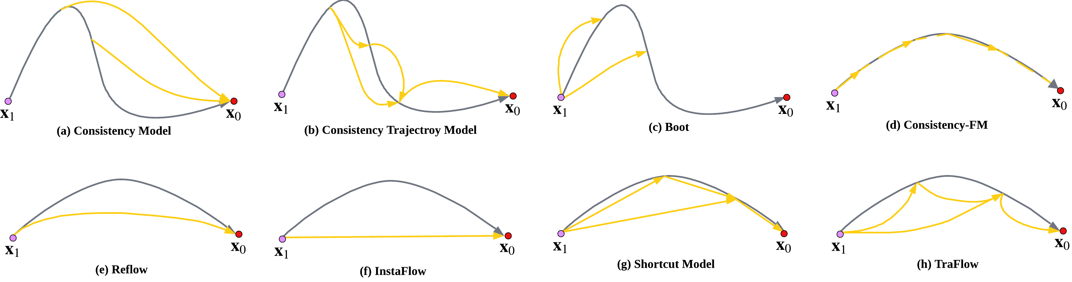
Figure 1: Visualisations on trajectory distillation methods. Grey arrows represent the trajectories of pre-trained models, whereas yellow arrows correspond to the trajectories of the distillation models. Panels (a-c) illustrate consistency distillation methods, while panels (d-h) depict rectified flow distillation methods. The trajectories in (a-c) exhibit greater curvature compared to those in (d-h), reflecting the fact that the pre-trained models in (a-c) are DMs, while those in (d-h) are rectified flows. In panels (b), (g), and (h), a single large step corresponds to the position of two smaller steps due to the self-consistency property of the trajectory.

5 Trajectory-based Distillation

Trajectory distillation considers the trajectory of a mapping between the noise distribution and the clean image distribution. In this section, we discuss two trajectory distillation types with different trajectory requirements: consistency distillation for the self-consistency property, and rectified flow distillation for straight trajectory. Figure 1 gives a simple visualization of these consistency distillation and rectified flow distillation models.

5.1 Consistency Distillation

Consistency model (CM) CM Song et al. (2023) is built based on the probability flow-ODE Song et al. (2021b). CM learns a consistency function $f_{{\boldsymbol{\mathbf{\phi}}}}({\boldsymbol{\mathbf{x}}}_{t},t)$ mapping an noisy image ${\boldsymbol{\mathbf{x}}}_{t}$ back to the clean image ${\boldsymbol{\mathbf{x}}}_{0}$ as:

$$f_{{\boldsymbol{\mathbf{\phi}}}}({\boldsymbol{\mathbf{x}}}_{t},t)={\boldsymbol{\mathbf{x}}}_{0}.$$ (17)

While the consistency model is required to satisfy the boundary condition at $t=0$, $f_{{\boldsymbol{\mathbf{\phi}}}}({\boldsymbol{\mathbf{x}}}_{t},t)$ is usually parameterized as:

$$f_{{\boldsymbol{\mathbf{\phi}}}}({\boldsymbol{\mathbf{x}}}_{t},t)=c_{\text{skip}}(t){\boldsymbol{\mathbf{x}}}_{t}+c_{\text{out}}(t)F_{{\boldsymbol{\mathbf{\phi}}}}({\boldsymbol{\mathbf{x}}}_{t},t),$$ (18)

where $F_{{\boldsymbol{\mathbf{\phi}}}}$ is the actual neural network to train, and $c_{\text{skip}}(t)$ and $c_{\text{out}}(t)$ are time-dependent factors such that $c_{\text{skip}}(0)=1,c_{\text{out}}(0)=0$.

While CM can be trained from scratch, a more popular choice for CM is to do distillation on pre-trained sampling trajectory, such as pre-trained DMs. In particular, the distillation objective function can be written as a distance metric between adjacent points as:

$$\mathcal{L}_{\text{CM}}=\mathbb{E}_{i}\left[\omega(t_{i})d({\boldsymbol{\mathbf{f}}}_{{\boldsymbol{\mathbf{\phi}}}}({\boldsymbol{\mathbf{x}}}_{t_{i}+\Delta t},t_{i}+\Delta t),{\boldsymbol{\mathbf{f}}}_{{\boldsymbol{\mathbf{\phi}}}^{-}}(\widehat{{\boldsymbol{\mathbf{x}}}}^{{\boldsymbol{\mathbf{\theta}}}}_{t_{i}},t_{i}))\right],$$ (19)

where $d(\cdot,\cdot)$ is a metric function, ${\boldsymbol{\mathbf{\phi}}}^{-}$ is the exponential moving average (EMA) of the past values ${\boldsymbol{\mathbf{\phi}}}$, and $\widehat{{\boldsymbol{\mathbf{x}}}}^{{\boldsymbol{\mathbf{\theta}}}}_{t_{i}}$ is obtained from pre-trained model as $\widehat{{\boldsymbol{\mathbf{x}}}}^{{\boldsymbol{\mathbf{\theta}}}}_{t_{i}}={\boldsymbol{\mathbf{x}}}_{t_{i}}-(t_{i}-t_{i+1})t_{i+1}\nabla_{{\boldsymbol{\mathbf{x}}}_{t_{i+1}}}\log p_{t_{i+1}}({\boldsymbol{\mathbf{x}}}_{t_{i+1}})$

Consistency Trajectory Model (CTM) CTM Kim et al. (2024) is introduced to minimize the accumulated estimation errors and discretization inaccuracies in multi-step consistency model sampling. While CM projects a noisy image ${\boldsymbol{\mathbf{x}}}_{t}$ to its clean image ${\boldsymbol{\mathbf{x}}}_{0}$, CTM extends it by designing a projection function which starts from time step $t$ to its later step $s(s<t)$ as:

$$f_{{\boldsymbol{\mathbf{\phi}}}}({\boldsymbol{\mathbf{x}}}_{t},t,s)=s/t\cdot{\boldsymbol{\mathbf{x}}}_{t}+(1-s)/t\cdot F_{{\boldsymbol{\mathbf{\phi}}}}({\boldsymbol{\mathbf{x}}}_{t},t,s).$$ (20)

where $F_{{\boldsymbol{\mathbf{\phi}}}}()$ is the actual neural networks to be optimized. Equation (21) ensures $f_{{\boldsymbol{\mathbf{\phi}}}}({\boldsymbol{\mathbf{x}}}_{t},t,s)$ satisfies the boundary condition when $f_{{\boldsymbol{\mathbf{\phi}}}}({\boldsymbol{\mathbf{x}}}_{t},t,1)={\boldsymbol{\mathbf{x}}}_{1}$.

Regarding loss function, CTM minimizes a soft consistency matching loss, which is defined as:

$$\mathcal{L}_{\text{CTM}}=\|f_{{\boldsymbol{\mathbf{\phi}}}}({\boldsymbol{\mathbf{x}}}_{t},t,s)-f_{\text{sg}({\boldsymbol{\mathbf{\phi}}})}(f_{{\boldsymbol{\mathbf{\theta}}}}({\boldsymbol{\mathbf{x}}}_{t},t,u),u,s)\|^{2},$$ (21)

where $0<s<u<t<1$, and $\text{sg}({\boldsymbol{\mathbf{\phi}}})$ is the EMA stop gradient operator. Equation (21) means that the one projected from the teacher model and the one from the student model should projected to the same value at the same time step.

Continuous-time Consistency Model Although most consistency models (CM) use discretized time steps for training, this approach often suffers from issues of tuning additional hyperparameters and inherently introduces discretization errors. Song and Dhariwal (2024); Geng et al. (2025); Lu and Song (2025) has been working on continuous-time CM and strategies to stablize its training. For example, Geng et al. (2025) analyses CM from a differential perspective and then progressively tightens the consistency condition, by letting the time different $\Delta t\to dt$ as training progresses. Lu and Song (2025) proposes a TrigFlow framework, which tries to unify the flow matching Lipman et al. (2023) and DMs, by defining the noisy image as ${\boldsymbol{\mathbf{x}}}_{t}=\cos(t){\boldsymbol{\mathbf{x}}}_{0}+\sin(t){\boldsymbol{\mathbf{\epsilon}}}$ for $t\in[0,\pi/2]$ and setting the training obejctive as:

$$\mathcal{L}_{\text{TrigFlow}}=\mathbb{E}_{{\boldsymbol{\mathbf{x}}}_{0},{\boldsymbol{\mathbf{z}}},t}\left[\|\sigma_{t}F_{{\boldsymbol{\mathbf{\phi}}}}({\boldsymbol{\mathbf{x}}}_{t}/\sigma_{t},t)-{\boldsymbol{\mathbf{x}}}_{t}\|^{2}\right].$$ (22)

where $F_{{\boldsymbol{\mathbf{\phi}}}}(\cdot)$ is the actual neural networks to be optimized.

5.2 Rectified Flow

Rectified Flow Rectified Flow Lipman et al. (2023); Liu et al. (2023b); Albergo et al. (2023), also named as flow matching or stochastic interpolation, leverage Ordinary Differential Equations (ODEs) to model the transition between two distributions, i.e., $p_{0}(\cdot),p_{1}(\cdot)$. Given a clean image ${\boldsymbol{\mathbf{x}}}_{0}\sim p_{0}({\boldsymbol{\mathbf{x}}}_{0})$ and a random noise ${\boldsymbol{\mathbf{x}}}_{1}\sim p_{1}({\boldsymbol{\mathbf{x}}}_{1})$, rectified flows construct a linear interpolation path defined as:

$${\boldsymbol{\mathbf{x}}}_{t}=t{\boldsymbol{\mathbf{x}}}_{1}+(1-t){\boldsymbol{\mathbf{x}}}_{0},\quad 0\leq t\leq 1.$$ (23)

The training objective for the model is formulated as:

$$\mathcal{L}_{\text{rf}}({\boldsymbol{\mathbf{\theta}}})=\int\mathbb{E}_{{\boldsymbol{\mathbf{x}}}_{1},{\boldsymbol{\mathbf{x}}}_{0}}\left[\|({\boldsymbol{\mathbf{x}}}_{1}-{\boldsymbol{\mathbf{x}}}_{0})-{\boldsymbol{\mathbf{v}}}_{{\boldsymbol{\mathbf{\theta}}}}({\boldsymbol{\mathbf{x}}}_{r},r)\|^{2}\right]dr,$$ (24)

where ${\boldsymbol{\mathbf{v}}}_{{\boldsymbol{\mathbf{\theta}}}}({\boldsymbol{\mathbf{x}}}_{t},t)$ represents the learned and pre-trained velocity field.

Given a random noise ${\boldsymbol{\mathbf{x}}}_{1}$, rectified flow’s new image generation process follows the ODE $d{\boldsymbol{\mathbf{x}}}_{t}={\boldsymbol{\mathbf{v}}}_{{\boldsymbol{\mathbf{\theta}}}}({\boldsymbol{\mathbf{x}}}_{t},t)\,dt,\quad t\in[0,1]$, where we can write the recovered clean image $\widehat{{\boldsymbol{\mathbf{x}}}}_{0}$ as $\widehat{{\boldsymbol{\mathbf{x}}}}_{0}={\boldsymbol{\mathbf{x}}}_{1}+\int_{1}^{0}{\boldsymbol{\mathbf{v}}}_{{\boldsymbol{\mathbf{\theta}}}}({\boldsymbol{\mathbf{x}}}_{r},r)dr$. Through minimizing $\mathcal{L}_{\text{rf}}$, the trained velocity field ${\boldsymbol{\mathbf{v}}}_{{\boldsymbol{\mathbf{\theta}}}}({\boldsymbol{\mathbf{x}}}_{t},t)$ is expected to approximate the direct path from ${\boldsymbol{\mathbf{x}}}_{1}$ to ${\boldsymbol{\mathbf{x}}}_{0}$. That is, rectified flows may be able to achieve high-quality data generation with fewer steps compared to traditional DMs, where the trajectory is usually curved and need more time steps to generate images.

Reflow vs InstaFlow In fact, while ${\boldsymbol{\mathbf{x}}}_{1}$ and ${\boldsymbol{\mathbf{x}}}_{0}$ are independently sampled from $p_{0}({\boldsymbol{\mathbf{x}}}_{0})$ and $p_{1}({\boldsymbol{\mathbf{x}}}_{1})$, simply training Equation (24) may not be able to obtain a straight trajectory. This is because the random pair $({\boldsymbol{\mathbf{x}}}_{1},{\boldsymbol{\mathbf{x}}}_{0})$ may provide highly noisy or even contradictory information regarding the direction between ${\boldsymbol{\mathbf{x}}}_{1}$ and ${\boldsymbol{\mathbf{x}}}_{0}$. Thus, Liu et al. (2023b) proposes a reflow mechanism, which first construct a data pair $({\boldsymbol{\mathbf{x}}}_{1},\widehat{{\boldsymbol{\mathbf{x}}}}_{0})$ from the pre-trained model ${\boldsymbol{\mathbf{v}}}_{{\boldsymbol{\mathbf{\theta}}}}({\boldsymbol{\mathbf{x}}}_{t},t)$, where $\widehat{{\boldsymbol{\mathbf{x}}}}_{0}$ is defined above as $\widehat{{\boldsymbol{\mathbf{x}}}}_{0}={\boldsymbol{\mathbf{x}}}_{1}+\int_{1}^{0}{\boldsymbol{\mathbf{v}}}_{{\boldsymbol{\mathbf{\theta}}}}({\boldsymbol{\mathbf{x}}}_{r},r)dr$, and then trains a new velocity ${\boldsymbol{\mathbf{v}}}_{{\boldsymbol{\mathbf{\phi}}}}({\boldsymbol{\mathbf{x}}}_{t},t)$ as:

$$\mathcal{L}_{\text{reflow}}= \int\mathbb{E}_{{\boldsymbol{\mathbf{x}}}_{1}}\left[\|({\boldsymbol{\mathbf{x}}}_{1}-\widehat{{\boldsymbol{\mathbf{x}}}}_{0})-{\boldsymbol{\mathbf{v}}}^{1}_{{\boldsymbol{\mathbf{\phi}}}}({\boldsymbol{\mathbf{x}}}_{t},t)\|^{2}\right]dt$$

$$= \int\mathbb{E}_{{\boldsymbol{\mathbf{x}}}_{1}}\left[\|\int_{1}^{0}{\boldsymbol{\mathbf{v}}}_{{\boldsymbol{\mathbf{\theta}}}}({\boldsymbol{\mathbf{x}}}_{r},r)dr-{\boldsymbol{\mathbf{v}}}^{1}_{{\boldsymbol{\mathbf{\phi}}}}({\boldsymbol{\mathbf{x}}}_{t},t)\|^{2}\right]dt,$$ (25)

where ${\boldsymbol{\mathbf{x}}}_{t}=(1-t)\widehat{{\boldsymbol{\mathbf{x}}}}_{0}+t{\boldsymbol{\mathbf{x}}}_{1}$.

On the other hand, InstaFlow Liu et al. (2023c); Zhu et al. (2025) aims to construct a one-step generator as ${\boldsymbol{\mathbf{x}}}_{1}+{\boldsymbol{\mathbf{v}}}_{{\boldsymbol{\mathbf{\phi}}}}({\boldsymbol{\mathbf{x}}}_{1},1)$, where ${\boldsymbol{\mathbf{v}}}_{{\boldsymbol{\mathbf{\phi}}}}({\boldsymbol{\mathbf{x}}}_{1},1)$ can be trained as

$$\mathcal{L}_{\text{rf-dis}}= \mathbb{E}_{{\boldsymbol{\mathbf{x}}}_{1}}\left[\|({\boldsymbol{\mathbf{x}}}_{1}-\widehat{{\boldsymbol{\mathbf{x}}}}_{0})-{\boldsymbol{\mathbf{v}}}^{1}_{{\boldsymbol{\mathbf{\phi}}}}({\boldsymbol{\mathbf{x}}}_{1},1)\|^{2}\right]$$

$$= \mathbb{E}_{{\boldsymbol{\mathbf{x}}}_{1}}\left[\|\int_{1}^{0}{\boldsymbol{\mathbf{v}}}_{{\boldsymbol{\mathbf{\theta}}}}({\boldsymbol{\mathbf{x}}}_{r},r)dr-{\boldsymbol{\mathbf{v}}}^{2}_{{\boldsymbol{\mathbf{\phi}}}}({\boldsymbol{\mathbf{x}}}_{1},1)\|^{2}\right].$$ (26)

In fact, we can see that ${\boldsymbol{\mathbf{v}}}_{{\boldsymbol{\mathbf{\phi}}}}({\boldsymbol{\mathbf{x}}}_{1},1)$ is learned to approximate the amount of velocity ${\boldsymbol{\mathbf{v}}}_{{\boldsymbol{\mathbf{\theta}}}}({\boldsymbol{\mathbf{x}}}_{r},r)$ changes from $t=1$ to $t=0$. Comparing these two distillation methods, reflow tries to obtain a new trajectory, where each time step’s velocity is close to constant, whereas instaflow tries to approximate the amount of changes given the random noise ${\boldsymbol{\mathbf{x}}}_{1}$.

5.3 Integrating Consistency Models and Rectified Flows

Consistency models and rectified flows each have distinct advantages and limitations. The former excels in regulating trajectory behavior, while the latter prioritizes achieving a straight trajectory.

Shortcut model Shortcut model Frans et al. (2025) is recently proposed as a promising improvement over the rectified flow. Shortcut model made two critical modifications to the existing rectified flow: (1) in addition to considering the current noisy image ${\boldsymbol{\mathbf{x}}}_{t}$ and its corresponding time step $t$, SM also takes the future projected time step $t+d$ as an input for the neural network ${\boldsymbol{\mathbf{v}}}({\boldsymbol{\mathbf{x}}}_{t},t,d)$. As a result, this future projected time step can help guide the generation of future noisy images; (2) Shortcut model also regulates the trajectory to be self-consistent. In particular, its loss function is:

$$\mathcal{L}_{\text{SM}}=\mathbb{E}_{{\boldsymbol{\mathbf{x}}}_{1},t,d}\left[\|({\boldsymbol{\mathbf{x}}}_{1}-\widehat{{\boldsymbol{\mathbf{x}}}}_{0})-{\boldsymbol{\mathbf{v}}}_{{\boldsymbol{\mathbf{\phi}}}}({\boldsymbol{\mathbf{x}}}_{t},t,0)\|^{2}\right.\\ \left.+\|{\boldsymbol{\mathbf{v}}}_{{\boldsymbol{\mathbf{\phi}}}}({\boldsymbol{\mathbf{x}}}_{t},t,2d)-\frac{{\boldsymbol{\mathbf{v}}}_{{\boldsymbol{\mathbf{\phi}}}}({\boldsymbol{\mathbf{x}}}_{t},t,d)+{\boldsymbol{\mathbf{v}}}_{{\boldsymbol{\mathbf{\phi}}}}({\boldsymbol{\mathbf{x}}}^{\prime}_{t+d},t,d)}{2}\|^{2}\right],$$ (27)

where ${\boldsymbol{\mathbf{x}}}^{\prime}_{t+d}={\boldsymbol{\mathbf{x}}}_{t}+{\boldsymbol{\mathbf{v}}}_{{\boldsymbol{\mathbf{\phi}}}}({\boldsymbol{\mathbf{x}}}_{t},t,d)$. The first term in Equation (27) enforces constant velocities, while the second term ensures the self-consistency of the generated trajectory.

Trajectory Distillation Flow (TraFlow) TraFlow Wu et al. (2025) also works to distill pre-trained rectified flows. Instead of approximating velocities, TraFlow uses neural networks to approximate the integration of velocities, which is $f_{{\boldsymbol{\mathbf{\phi}}}}({\boldsymbol{\mathbf{x}}}_{t},t,s)={\boldsymbol{\mathbf{x}}}_{t}+\int_{t}^{s}{\boldsymbol{\mathbf{v}}}_{{\boldsymbol{\mathbf{\theta}}}}({\boldsymbol{\mathbf{x}}}_{r},r)dr$. The loss function of TraFlow considers the factors of soft consistency matching and trajectory straightness:

$$\mathcal{L}_{\text{TraFlow}}=\int\mathbb{E}_{{\boldsymbol{\mathbf{x}}}_{1}}\left[\|({\boldsymbol{\mathbf{x}}}_{1}-\widehat{{\boldsymbol{\mathbf{x}}}}_{0})-\frac{\partial f_{{\boldsymbol{\mathbf{\phi}}}}({\boldsymbol{\mathbf{x}}}_{t},t,t+\Delta t)}{\partial\Delta t}\|^{2}\right]\\ +\|f_{{\boldsymbol{\mathbf{\phi}}}}({\boldsymbol{\mathbf{x}}}_{t},t,s)-f_{\text{sg}({\boldsymbol{\mathbf{\phi}}})}(f_{{\boldsymbol{\mathbf{\theta}}}}({\boldsymbol{\mathbf{x}}}_{t},t,u),u,s)\|^{2}ds.$$ (28)

Since TraFlow directly projects the noisy image at a future time step $s$, it removes the need for an ODE solver to approximate the trajectory, thereby avoiding approximation errors.

In fact, both Shortcut model and TraFlow share the same motivation and even model structure with CTM Kim et al. (2024), which take the noisy image ${\boldsymbol{\mathbf{x}}}_{t}$, the current time step $t$, and the future time step $s$ or the step lag $s-t$ as inputs. Integrating the consistency model with trajectory straightness is a natural choice, as a straight trajectory is inherently self-consistent.

Consistency-FM Instead of requiring the trajectory to be self-consistent, Consistency-FM Yang et al. (2024) works on the velocity side by setting consistent velocities. In particular, consistency-FM derives the equivalence between two conditions at any two time steps $\forall t,s\in[0,1]$:

condition 1: $${\boldsymbol{\mathbf{v}}}({\boldsymbol{\mathbf{x}}}_{t},t)={\boldsymbol{\mathbf{v}}}({\boldsymbol{\mathbf{x}}}_{s},s);$$

condition 2: $${\boldsymbol{\mathbf{x}}}_{t}+(1-t){\boldsymbol{\mathbf{v}}}({\boldsymbol{\mathbf{x}}}_{t},t)={\boldsymbol{\mathbf{x}}}_{s}+(1-s){\boldsymbol{\mathbf{v}}}({\boldsymbol{\mathbf{x}}}_{s},s),$$ (29)

in which condition 1 means the velocities at any time steps are the same and condition 2 refers to that the linearly projected points from different time steps would be the same. Consistency-FM set the training objective as to let the velocity satisfies these two conditions. Consistency-FM also develops multi-segment mechanism to further improve the model performance.

6 Adversarial Loss

Diffusion-GAN Wang et al. (2023); Xu et al. (2024) may be the first introducing the adversarial loss Goodfellow et al. (2014) in training DMs. Diffusion-GAN optimizes a min-max objective function to obtain an optmized DM:

$$\mathcal{L}_{\text{Diffusion-GAN}}=\mathbb{E}_{t,{\boldsymbol{\mathbf{x}}}_{t}\sim q({\boldsymbol{\mathbf{x}}}|{\boldsymbol{\mathbf{x}}}_{0},t)}\left[\log\mathcal{D}_{{\boldsymbol{\mathbf{\psi}}}}({\boldsymbol{\mathbf{x}}}_{t})\right]\\ +\mathbb{E}_{t,{\boldsymbol{\mathbf{z}}}\sim p({\boldsymbol{\mathbf{z}}}),{\boldsymbol{\mathbf{x}}}^{\prime}_{t}\sim q({\boldsymbol{\mathbf{x}}}^{\prime}_{t}|f_{{\boldsymbol{\mathbf{\phi}}}}({\boldsymbol{\mathbf{z}}}),t)}\left[\log(1-\mathcal{D}_{{\boldsymbol{\mathbf{\psi}}}}({\boldsymbol{\mathbf{x}}}^{\prime}_{t}))\right],$$ (30)

where $\mathcal{D}_{{\boldsymbol{\mathbf{\psi}}}}(\cdot)$ is the classifier for the adversarial loss. Consequently, the training process involves alternating optimization of the generator’s parameters, ${\boldsymbol{\mathbf{\phi}}}$, and the classifier’s parameters, ${\boldsymbol{\mathbf{\psi}}}$.

In addition to direct training, adversarial loss itself can be independently used as adversarial distribution distillation (ADD) Sauer et al. (2025), in which the loss function is in the GAN format:

$$\mathcal{L}_{\text{ADD}}=\mathbb{E}_{t,{\boldsymbol{\mathbf{z}}}\sim p({\boldsymbol{\mathbf{z}}}),{\boldsymbol{\mathbf{x}}}^{\prime}_{t}\sim q({\boldsymbol{\mathbf{x}}}^{\prime}_{t}|f_{{\boldsymbol{\mathbf{\phi}}}}({\boldsymbol{\mathbf{z}}}),t)}\left[\log\mathcal{D}_{{\boldsymbol{\mathbf{\psi}}}}({\boldsymbol{\mathbf{x}}}_{t})\right.\\ \left.+\log(1-\mathcal{D}_{{\boldsymbol{\mathbf{\psi}}}}({\boldsymbol{\mathbf{x}}}^{\prime}_{t}))\right].$$ (31)

ADD is successfully used for SDXL Turbo Sauer et al. (2024), a text-to-image model that enables realtime generation.

Since this adversarial loss is orthogonal to existing methods, common distillation methods can include it as an additional technique to improve the distillation performance Zhou et al. (2025b). When real data is available, the performance of the student model might surpass that of the teacher model.

7 Challenges and Future Direction

Although pre-trained DM distillation methods have made significant progress, this field still faces substantial challenges, along with promising future directions for addressing them.

7.1 Challenges

1, Training on large pre-trained models Most experiments evaluating the effectiveness of distillation methods are conducted on small datasets, such as CIFAR-10 and ImageNet. However, distilling large-scale pre-trained DMs, such as Stable Diffusion Rombach et al. (2022); Esser et al. (2024), remains computationally demanding and is infeasible for research groups with limited GPU access. Therefore, developing computationally efficient approaches for distilling such large-scale models is a critical and promising research direction.

2, Trade-off between quality and speed Distillation methods accelerate sampling by reducing the number of required function evaluations or sampling steps. As a result, their aggressive reduction might lead to degraded sample quality due to the accummulated errors. Obtaining an optimal balance is necessary for carefully designed approximations, improved training objectives, and architectural modifications to mitigate artifacts introduced by accelerated sampling. Understanding this trade-off is crucial for advancing efficient diffusion-based generative models that retain high fidelity while being computationally feasible for real-world applications.

3, Training guidelines The lack of uniform training guidelines for DM distillation creates inconsistencies in methodology and evaluation. While it is common to adopt the settings of EDM Karras et al. (2022, 2024) to train DMs, key distillation aspects, such as weight functions, network structures, and distillation stages, vary across studies without a standardized framework. Different weight functions alter training dynamics, while architectural choices and stage configurations affect efficiency and fidelity. Without clear guidelines, comparing methods fairly and reproducing results remains challenging.

7.2 Future directions

1, Training smaller-size student model Most existing approaches primarily focus on reducing the number of time steps to achieve high-quality image generation. However, they often overlook effective strategies for reducing model size, specifically the neural network’s capacity. Employing a smaller student model is particularly beneficial for practical applications, such as fast sampling and adaptability to low-resource environments. SlimFlow Zhu et al. (2025) explores this direction by leveraging annealing to reduce model size, but further investigation is required.

2, Trajectory optimization Optimizing the trajectory between random noise and clean images remains a crucial area of research, particularly with the advancement of consistency models and rectified flows. Current approaches primarily focus on enforcing self-consistency and trajectory straightness. However, further exploration of alternative trajectory properties could provide valuable insights for enhancing both the efficiency and quality of sampling.

3, Student model initialization The parameters of the student distillation model are typically initialized using those of the teacher model. However, the two models are designed with different objectives and sampling mechanisms. For instance, a student model with only a few sampling steps can be viewed as an integration of a teacher model with $1\,000$ sampling steps. While effective initialization can accelerate student model training, the development of a universal initialization strategy remains an open research question.

4, Theoretical understanding of using distillation There is a question of whether distillation is necessary to achieve such models or if they could be trained directly. While the existence of a distilled model demonstrates feasibility, it does not ensure optimal efficiency in achieving it. Some models obtained through diffusion distillation can, in principle, be trained from scratch, though this approach generally underperforms compared to distillation, reflecting the well-established advantage of distilling large neural networks into smaller ones. This analogy holds for DMs, where distillation compresses a deep sampling process into a shallower one. Consistency models might offer an example where both distillation and direct training are possible, but the latter requires careful hyperparameter tuning and training strategies. In additional to these empirical evidence, a theoretical understanding for the advantages of distillation methods would be interesting to explore in the future.

5, Broader applications of distillation methods This survey primarily focuses on the methodological aspects of distillation techniques and does not address practical applications such as text-to-image synthesis. Given the demonstrated effectiveness of DMs in fields like image, audio, and video generation, it would be exciting to explore further applications in these domains and beyond. Particularly, the unique advantages of distillation methods in adapting to low computational resource environments present significant potential for broader application.

References

- Albergo et al. [2023] Michael S Albergo, Nicholas M Boffi, and Eric Vanden-Eijnden. Stochastic Interpolants: A Unifying Framework for Flows and Diffusions. arXiv preprint arXiv:2303.08797, 2023.
- Berthelot et al. [2023] David Berthelot, Arnaud Autef, Jierui Lin, Dian Ang Yap, Shuangfei Zhai, Siyuan Hu, Daniel Zheng, Walter Talbott, and Eric Gu. Tract: Denoising Diffusion Models with Transitive Closure Time-Distillation. arXiv preprint arXiv:2303.04248, 2023.
- Dieleman [2024] Sander Dieleman. The paradox of diffusion distillation, 2024.
- Esser et al. [2024] Patrick Esser, Sumith Kulal, Andreas Blattmann, Rahim Entezari, Jonas Müller, Harry Saini, Yam Levi, Dominik Lorenz, Axel Sauer, Frederic Boesel, et al. Scaling Rectified Rlow Transformers for High-Resolution Image Synthesis. ICML, 2024.
- Evans et al. [2024] Zach Evans, CJ Carr, Josiah Taylor, Scott H Hawley, and Jordi Pons. Fast Timing-Conditioned Latent Audio Diffusion. ICML, 2024.
- Frans et al. [2025] Kevin Frans, Danijar Hafner, Sergey Levine, and Pieter Abbeel. One Step Diffusion via Shortcut Models. ICLR, 2025.
- Geng et al. [2025] Zhengyang Geng, Ashwini Pokle, William Luo, Justin Lin, and J Zico Kolter. Consistency Models Made Easy. ICLR, 2025.
- Goodfellow et al. [2014] Ian Goodfellow, Jean Pouget-Abadie, Mehdi Mirza, Bing Xu, David Warde-Farley, Sherjil Ozair, Aaron Courville, and Yoshua Bengio. Generative Adversarial Networks. NeurIPS, 2014.
- Gu et al. [2023] Jiatao Gu, Shuangfei Zhai, Yizhe Zhang, Lingjie Liu, and Joshua M Susskind. Boot: Data-free distillation of denoising diffusion models with bootstrapping. ICML 2023, 2023.
- Ho et al. [2020a] Jonathan Ho, Ajay Jain, and Pieter Abbeel. Denoising Diffusion Probabilistic Models. NeurIPS, 2020.
- Ho et al. [2020b] Jonathan Ho, Ajay Jain, and Pieter Abbeel. Denoising Diffusion Probabilistic Models. NeurIPS, 2020.
- Huang et al. [2024] Yi Huang, Jiancheng Huang, Yifan Liu, Mingfu Yan, Jiaxi Lv, Jianzhuang Liu, Wei Xiong, He Zhang, Shifeng Chen, and Liangliang Cao. Diffusion Model-based Image Editing: A Survey. arXiv preprint arXiv:2402.17525, 2024.
- Karras et al. [2022] Tero Karras, Miika Aittala, Timo Aila, and Samuli Laine. Elucidating the Design Space of Diffusion-based Generative Models. NeurIPS, 2022.
- Karras et al. [2024] Tero Karras, Miika Aittala, Jaakko Lehtinen, Janne Hellsten, Timo Aila, and Samuli Laine. Analyzing and Improving the Training Dynamics of Diffusion Models. CVPR, 2024.
- Kim et al. [2024] Dongjun Kim, Chieh-Hsin Lai, Wei-Hsiang Liao, Naoki Murata, Yuhta Takida, Toshimitsu Uesaka, Yutong He, Yuki Mitsufuji, and Stefano Ermon. Consistency Trajectory Models: Learning Probability Flow ODE Trajectory of Diffusion. ICLR, 2024.
- Liang et al. [2024] Yixun Liang, Xin Yang, Jiantao Lin, Haodong Li, Xiaogang Xu, and Yingcong Chen. LucidDreamer: Towards High-Fidelity Text-to-3D Generation via Interval Score Matching. CVPR, 2024.
- Lipman et al. [2023] Yaron Lipman, Ricky TQ Chen, Heli Ben-Hamu, Maximilian Nickel, and Matt Le. Flow Matching for Generative Modeling. ICLR, 2023.
- Liu et al. [2023a] Haohe Liu, Zehua Chen, Yi Yuan, Xinhao Mei, Xubo Liu, Danilo Mandic, Wenwu Wang, and Mark D Plumbley. Audioldm: Text-to-Audio Generation with Latent Diffusion Models. ICML, 2023.
- Liu et al. [2023b] Xingchao Liu, Chengyue Gong, and qiang liu. Flow Straight and Fast: Learning to Generate and Transfer Data with Rectified Flow. 2023.
- Liu et al. [2023c] Xingchao Liu, Xiwen Zhang, Jianzhu Ma, Jian Peng, et al. Instaflow: One Step is Enough for High-quality Diffusion-based Text-to-image Generation. ICLR, 2023.
- Lu and Song [2025] Cheng Lu and Yang Song. Simplifying, Stabilizing and Scaling Continuous-time Consistency Models. ICLR, 2025.
- Luhman and Luhman [2021] Eric Luhman and Troy Luhman. Knowledge Distillation in Iterative Generative Models for Improved Sampling Speed. arXiv preprint arXiv:2101.02388, 2021.
- Lukoianov et al. [2024] Artem Lukoianov, Haitz Sáez de Ocáriz Borde, Kristjan Greenewald, Vitor Campagnolo Guizilini, Timur Bagautdinov, Vincent Sitzmann, and Justin Solomon. Score Distillation via Reparametrized DDIM. arXiv preprint arXiv:2405.15891, 2024.
- Luo et al. [2024a] Weijian Luo, Tianyang Hu, Shifeng Zhang, Jiacheng Sun, Zhenguo Li, and Zhihua Zhang. Diff-Instruct: A Universal Approach for Transferring Knowledge From Pre-trained Diffusion Models. NeurIPS, 2024.
- Luo et al. [2024b] Weijian Luo, Zemin Huang, Zhengyang Geng, J Zico Kolter, and Guo-jun Qi. One-Step Diffusion Distillation through Score Implicit Matching. arXiv preprint arXiv:2410.16794, 2024.
- Luo [2023] Weijian Luo. A Comprehensive Survey on Knowledge Kistillation of Diffusion Models. arXiv preprint arXiv:2304.04262, 2023.
- Meng et al. [2023] Chenlin Meng, Robin Rombach, Ruiqi Gao, Diederik Kingma, Stefano Ermon, Jonathan Ho, and Tim Salimans. On Distillation of Guided Diffusion Models. CVPR, 2023.
- Nguyen and Tran [2024] Thuan Hoang Nguyen and Anh Tran. Swiftbrush: One-Step Text-to-Image Diffusion Model with Variational Score Distillation. CVPR, 2024.
- Poole et al. [2023] Ben Poole, Ajay Jain, Jonathan T Barron, and Ben Mildenhall. Dreamfusion: Text-to-3D using 2D Diffusion. ICLR, 2023.
- Rombach et al. [2022] Robin Rombach, Andreas Blattmann, Dominik Lorenz, Patrick Esser, and Björn Ommer. High-resolution Image Synthesis with Latent Diffusion Models. CVPR, 2022.
- Salimans and Ho [2022] Tim Salimans and Jonathan Ho. Progressive Distillation for Fast Sampling of Diffusion Models. ICLR, 2022.
- Sauer et al. [2024] Axel Sauer, Frederic Boesel, Tim Dockhorn, Andreas Blattmann, Patrick Esser, and Robin Rombach. Fast High-Resolution Image Synthesis with Latent Adversarial Diffusion Distillation. SIGGRAPH, 2024.
- Sauer et al. [2025] Axel Sauer, Dominik Lorenz, Andreas Blattmann, and Robin Rombach. Adversarial Diffusion Distillation. ECCV, 2025.
- Shuai et al. [2024] Xincheng Shuai, Henghui Ding, Xingjun Ma, Rongcheng Tu, Yu-Gang Jiang, and Dacheng Tao. A Survey of Multimodal-Guided Image Editing with Text-to-Image Diffusion Models. arXiv preprint arXiv:2406.14555, 2024.
- Song and Dhariwal [2024] Yang Song and Prafulla Dhariwal. Improved Techniques for Training Consistency Models. ICLR, 2024.
- Song et al. [2021a] Jiaming Song, Chenlin Meng, and Stefano Ermon. Denoising Diffusion Implicit Models. ICLR, 2021.
- Song et al. [2021b] Yang Song, Jascha Sohl-Dickstein, Diederik P Kingma, Abhishek Kumar, Stefano Ermon, and Ben Poole. Score-based Generative Modeling through Stochastic Differential Equations. ICLR, 2021.
- Song et al. [2023] Yang Song, Prafulla Dhariwal, Mark Chen, and Ilya Sutskever. Consistency Models. ICML, 2023.
- Wang et al. [2023] Zhendong Wang, Huangjie Zheng, Pengcheng He, Weizhu Chen, and Mingyuan Zhou. Diffusion-GAN: Training GANs with Diffusion. ICLR, 2023.
- Wang et al. [2024] Zhengyi Wang, Cheng Lu, Yikai Wang, Fan Bao, Chongxuan Li, Hang Su, and Jun Zhu. Prolificdreamer: High-Fidelity and Diverse Text-to-3D Generation with Variational Score Distillation. NeurIPS, 2024.
- Watson et al. [2023] Joseph L Watson, David Juergens, Nathaniel R Bennett, Brian L Trippe, Jason Yim, Helen E Eisenach, Woody Ahern, Andrew J Borst, Robert J Ragotte, Lukas F Milles, et al. De novo design of protein structure and function with RFdiffusion. Nature, 2023.
- Wu et al. [2023] Yusong Wu, Ke Chen, Tianyu Zhang, Yuchen Hui, Taylor Berg-Kirkpatrick, and Shlomo Dubnov. Large-scale Contrastive Language-Audio Pretraining with Feature Fusion and Keyword-to-Caption Augmentation. ICASSP, 2023.
- Wu et al. [2024] Kevin E Wu, Kevin K Yang, Rianne van den Berg, Sarah Alamdari, James Y Zou, Alex X Lu, and Ava P Amini. Protein Structure Generation via Folding Diffusion. Nature Communications, 2024.
- Wu et al. [2025] Zhangkai Wu, Xuhui Fan, Hongyu Wu, and Longbing Cao. Traflow: Trajectory Distillation on Pre-Trained Rectified Flow. arXiv preprint, 2025.
- Xie et al. [2024] Sirui Xie, Zhisheng Xiao, Diederik P Kingma, Tingbo Hou, Ying Nian Wu, Kevin Patrick Murphy, Tim Salimans, Ben Poole, and Ruiqi Gao. Em Distillation for One-Step Diffusion Models. NeurIPS, 2024.
- Xu et al. [2024] Yanwu Xu, Yang Zhao, Zhisheng Xiao, and Tingbo Hou. UFOGen: You Forward Once Large Scale Text-to-Image Generation via Diffusion GANs. CVPR, 2024.
- Yang et al. [2022] Ling Yang, Zhilong Zhang, Yang Song, Shenda Hong, Runsheng Xu, Yue Zhao, Yingxia Shao, Wentao Zhang, Bin Cui, and Ming-Hsuan Yang. Diffusion Models: A Comprehensive Survey of Methods and Applications. arXiv preprint arXiv:2209.00796, 2022.
- Yang et al. [2024] Ling Yang, Zixiang Zhang, Zhilong Zhang, Xingchao Liu, Minkai Xu, Wentao Zhang, Chenlin Meng, Stefano Ermon, and Bin Cui. Consistency Flow Matching: Defining Straight Flows with Velocity Consistency. arXiv preprint arXiv:2407.02398, 2024.
- Yim et al. [2023] Jason Yim, Brian L Trippe, Valentin De Bortoli, Emile Mathieu, Arnaud Doucet, Regina Barzilay, and Tommi Jaakkola. SE(3) Diffusion Model with Application to Protein Backbone Generation. arXiv preprint arXiv:2302.02277, 2023.
- Yin et al. [2024a] Tianwei Yin, Michaël Gharbi, Taesung Park, Richard Zhang, Eli Shechtman, Fredo Durand, and William T Freeman. Improved Distribution Matching Distillation for Fast Image Synthesis. NeurIPS, 2024.
- Yin et al. [2024b] Tianwei Yin, Michaël Gharbi, Richard Zhang, Eli Shechtman, Fredo Durand, William T Freeman, and Taesung Park. One-Step Diffusion with Distribution Matching Distillation. CVPR, 2024.
- Zhou et al. [2024] Mingyuan Zhou, Huangjie Zheng, Zhendong Wang, Mingzhang Yin, and Hai Huang. Score identity distillation: Exponentially fast distillation of pretrained diffusion models for one-step generation. In ICML, 2024.
- Zhou et al. [2025a] Mingyuan Zhou, Zhendong Wang, Huangjie Zheng, and Hai Huang. Long and Short Guidance in Score identity Distillation for One-Step Text-to-Image Generation. ICLR, 2025.
- Zhou et al. [2025b] Mingyuan Zhou, Huangjie Zheng, Yi Gu, Zhendong Wang, and Hai Huang. Adversarial Score identity Distillation: Rapidly Surpassing the Teacher in One Step. ICLR, 2025.
- Zhu et al. [2025] Yuanzhi Zhu, Xingchao Liu, and Qiang Liu. Slimflow: Training Smaller One-Step Diffusion Models with Rectified Flow. ECCV, 2025.