Privacy amplification by random allocation

Abstract

We consider the privacy guarantees of an algorithm in which a user’s data is used in $k$ steps randomly and uniformly chosen from a sequence (or set) of $t$ differentially private steps. We demonstrate that the privacy guarantees of this sampling scheme can be upper bound by the privacy guarantees of the well-studied independent (or Poisson) subsampling in which each step uses the user’s data with probability $(1+o(1))k/t$. Further, we provide two additional analysis techniques that lead to numerical improvements in some parameter regimes. The case of $k=1$ has been previously studied in the context of DP-SGD in Balle et al. (2020) and very recently in Chua et al. (2024a). Privacy analysis of Balle et al. (2020) relies on privacy amplification by shuffling which leads to overly conservative bounds. Privacy analysis of Chua et al. (2024a) relies on Monte Carlo simulations that are computationally prohibitive in many practical scenarios and have additional inherent limitations.

1 Introduction

One of the central tools in the analysis of differentially private algorithms are so-called privacy amplification results where amplification results from sampling of the inputs. In these results one starts with a differentially private algorithms (or a sequence of such algorithms) and a randomized algorithm for selecting (or sampling) which of the $n$ elements in a dataset to run each of the $t$ algorithms on. Importantly, the random bits of the sampling scheme and the selected data elements are not revealed. For a variety of sampling schemes this additional uncertainty is known to lead to improved privacy guarantees of the resulting algorithm, that it, privacy amplification.

In the simpler, single step, case a DP algorithm is run on a randomly chosen subset of the dataset. As first shown by Kasiviswanathan et al. (2011), if each element of the dataset is included in the subset with probability $\lambda$ (independently of other elements) then the privacy of the resulting algorithm is better (roughly) by a factor $\lambda$. This basic result has found numerous applications, most notably in the analysis of the differentially private stochastic gradient descent (DP-SGD) algorithm (Bassily et al., 2014). In DP-SGD gradients are computed on randomly chosen batches of data points and then privatized through Gaussian noise addition. Privacy analysis of this algorithm is based on the so called Poisson sampling: elements in each batch and across batches are chosen randomly and independently of each other. The absence of dependence implies that the algorithm can be analyzed relatively easily as a direct composition of single step amplification results. The downside of this simplicity is that such sampling is less efficient and harder to implement within the standard ML pipelines. As a result, in practice some form of shuffling is used to define the batches in DP-SGD leading to a well-recognized discrepancy between the implementations of DP-SGD and their analysis (Chua et al., 2024b, c; Annamalai et al., 2024).

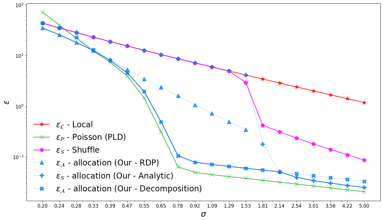
Figure 1: Upper bounds on privacy parameter $\epsilon$ as a function of the noise parameter $\sigma$ for various schemes and the local mechanism (no amplification), all using the Gaussian mechanism with fixed parameters $\delta=10^{-10}$, $t=10^{6}$. In the Poisson scheme $\lambda=1/t$. The missing part of the RDP based calculation is due to computational limitations.

Motivated by the shuffle model of federated data analysis (Bittau et al., 2017), Cheu et al. (2019); Erlingsson et al. (2019) have studied the privacy amplification of the shuffling scheme. In this scheme the $n$ elements are randomly and uniformly permuted and $i$-th element in the permuted order is used in the $i$-th step of the algorithm. This sampling scheme can be used to analyze the implementations of DP-SGD used in practice (Erlingsson et al., 2019; Feldman et al., 2021). However, the analysis of this sampling scheme is more involved and nearly tight results are known only for relatively simple pure DP ($\delta=0$) algorithms (Feldman et al., 2021, 2023; Girgis et al., 2021). In particular, applying these results to Gaussian noise addition requires using $(\epsilon,\delta)$-guarantees of the Gaussian noise. This leads to an additional $\sqrt{\ln(1/\delta)}$ factor in the asymptotic analysis and significantly worse numerical results (see Fig. 1 for comparison).

Note that shuffling differs from Poisson subsampling in that participation of elements is dependent both in each step (or batch) and across the steps. If the participation of elements in each step is dependent (by fixing the total number of participating elements) but the steps are independent then the sampling scheme can be tightly analyzed as direct composition of fixed subset size sampling steps (e.g., using bound in Balle et al. (2018); Zhu et al. (2022)). However a more problematic aspect of Poisson sampling is the stochasticity in the number of times each element is used in all steps. For example, using Poisson sampling with sampling rate $1/t$ over $t$ batches will result in roughly $1/e$ probability of not using the sample which implies dropping approximately $37\%$ of the data. In the distributed setting it is also often necessary to limit the maximum number of times a user participates in the analysis due to time or communication constraints (Chen et al., 2024). Poisson sampling does not allow to fully exploit the available limit potentially hurting the utility.

Therefore here we analyze sample schemes in which participation of elements in each step is independent but each element participates in $k$ randomly chosen steps (out of the total $t$). We refer to this sampling as $k$ out of $t$ random allocation. For $k=1$ this scheme is a special case of the random check-in model of defining batches for DP-SGD in (Balle et al., 2020). Their analysis of this variant relies on the amplification properties of shuffling and thus does not lead to better privacy guarantees than those that are known for shuffling. Very recently, Chua et al. (2024a) have studied such sampling (referring to it as balls-and-bins sampling) in the context of training neural networks via DP-SGD. Their main results show that from the point of view of utility (namely, accuracy of the final model) random allocation is essentially identical to shuffling and is noticeably better than Poisson sampling. Their privacy analysis reduces the problem to analyzing the divergence of a specific pair of distributions on $\mathbb{R}^{t}$. They then use Monte Carlo simulations to estimate the privacy parameters of this pair. Their numerical results suggest that privacy guarantees of $k=1$ random allocation are similar to those of the Poisson sampling with rate of $1/t$. While very encouraging, such simulations have several limitations, most notably, achieving high confidence estimates for small $\delta$ and supporting composition appear to be computationally impractical. This approach also does not lead to provable privacy guarantees and does not lend itself to asymptotic analysis (such as the scaling of the privacy guarantees with $t$).

1.1 Our contribution

We provide three new analyses for of the random allocation setting that result in provable guarantees that nearly match or exceed those of the Poisson subsampling at rate $k/t$. The analyses rely on different techniques and lead to incomparable numerical results. We describe the specific results below and illustrate the resulting bounds in Fig. 1.

In our main result we show that the privacy of random allocation is upper bounded by that of the Poisson scheme with sampling probability $\approx k/t$ up to lower order terms which are asymptotically vanishing in $t/k$. Specifically, we upper bound it by the $k$-wise composition of Poisson subsampling with rate $(1+\gamma)k/t$ applied to a dominating pair of distributions for the original algorithm (Def. 2.11) with an additional $t\delta_{0}+\delta^{\prime}$ added to the $\delta$ parameter. Here, $\gamma=O\left(e^{\epsilon_{0}}\sqrt{\frac{k\ln(k/\delta^{\prime})}{t}}\right)$ and $\epsilon_{0},\delta_{0}$ are the privacy parameters of the original algorithm. The formal statement of this result that includes all the constants can be found in Thm. 3.2.

We note that our result relies on $\epsilon_{0},\delta_{0}$ parameters of the original algorithm. This may appear to lead to the same overheads as the results based on full shuffling analysis. However in our case these parameters only affect the lower order term, whereas for shuffling they are used as the basis for privacy amplification.

Our analysis relies on several simplification steps. Given a dominating pair of distributions for the original algorithm, we first derive an explicit dominating pair of distributions for random allocation (extending a similar result for Gaussian noise in (Chua et al., 2024a)). Equivalently we reduce the allocation for general multi-step adaptive algorithms to the analysis of random allocation for a single (non-adaptive) randomizer on two inputs. We also analyze only the case of $k=1$ and then use a reduction from general $k$ to $k=1$. This reduction relies on the recent concurrent composition results (Lyu, 2022; Vadhan & Zhang, 2023). Finally, our analysis of the non-adaptive randomizer for $k=1$ relies on a decomposition of the allocation scheme into a sequence of posterior sampling steps for which we then prove an upper bound on subsampling probability.

We note that, in general, the privacy of the composition of subsampling of the dominating pair of distributions can be worse than the privacy of the Poisson subsampling. However, all existing analyses of the Poisson sampling are effectively based on composition of subsampling for a dominating pair of distributions. Moreover, if the algorithm has a worst case input for which deletion leads to a dominating pair of distributions then our upper bound can be stated directly in terms of the entire Poisson subsampling scheme. Such dominating input exists for many standard algorithms including those based on Gaussian and Laplace noise addition.

While our result shows asymptotic equivalence of allocation and Poisson subsampling, it may lead to suboptimal bounds for small values of $t/k$ and large $\epsilon_{0}$. We address this using two additional techniques.

We first show that $\epsilon$ of random allocation with $k=1$ is at most a constant ($\approx 1.6$) factor times larger than $\epsilon$ of the Poisson sampling with rate $1/t$ for the same $\delta$ (see Theorem 4.1). This upper bound does not asymptotically approach Poisson subsampling but applies in all parameter regimes. To prove this upper bound we observe that Poisson subsampling is essentially a mixture of random allocation schemes with various values of $k$. We then prove a monotonicity property of random allocations showing that increasing $k$ leads to worse privacy. Combining these results with with the advanced joint convexity Balle et al. (2018) gives the upper bound.

Finally, we derive a closed form expression for the Renyi DP (Mironov, 2017) of the dominating pair of distributions for allocation in terms of the RDP parameters of the original algorithm (Theorem 4.6). This method has two important advantages. First it gives a precise bound on the RDP parameters of integer order (as opposed to just an upper bound). Secondly, it is particularly easy to use in the typical setting where composition is used in addition to a sampling scheme (for example when $k>1$ or in multi-epoch DP-SGD). The primary disadvantage of this technique is that the conversion from RDP bounds to the regular $(\epsilon,\delta)$ bounds is known to be somewhat lossy. The same loss is also incurred when Poisson sampling is analyzed via RDP (referred to as moment accounting (Abadi et al., 2016)). The loss is typically within $10-20\%$ range in multi-epoch settings. In our evaluations of this method for Gaussian distribution in most regimes the resulting bounds are almost indistinguishable from those obtained via RDP for Poisson distribution (see Fig. 2 for examples). In fact, in some regimes it is better than Poisson sampling (Figure 3).

1.2 Related work

Our work builds heavily on tools and ideas developed for analysis of privacy amplification by subsampling, composition and shuffling. We have covered the work directly related to ours earlier and will describe some of the tools and their origins in the preliminaries. A more detailed technical and historical overview of subsampling and composition for DP can be found in the survey by Steinke (2022). The shuffle model was first proposed by Bittau et al. (2017). The formal analysis of the privacy guarantees in this model was initiated in (Erlingsson et al., 2019; Cheu et al., 2019). Erlingsson et al. (2019) defined the sequential shuffling scheme that we discuss here and proved the first general privacy amplification results for this scheme albeit only for pure DP algorithms. Improved analyses and extensions to approximate DP were given in (Balle et al., 2019, 2020; Feldman et al., 2021, 2023; Girgis et al., 2021; Koskela et al., 2022).

DP-SGD was first defined and theoretically analyzed in the convex setting by Bassily et al. (2014). Its use in machine learning was spearheaded by the landmark work of Abadi et al. (2016) who significantly improved the privacy analysis via the moments accounting technique and demonstrated the practical utility of the approach. In addition to a wide range of practical applications, this work has motivated the development of more advanced techniques for analysis of sampling and composition. At the same time most analyses used in practice still assume Poisson subsampling when selecting batches whereas some type of shuffling is used in implementation. It was recently shown that it results in an actual difference between the reported and true privacy level in some regimes (Chua et al., 2024b, c; Annamalai et al., 2024).

2 Preliminaries

We denote the domain of elements by $\mathcal{X}$ and the set of possible outputs by $\mathcal{O}$. We describe a sequence of possibly adaptively chosen algorithms using a randomized algorithm $M:\mathcal{X}^{*}\times\mathcal{O}^{*}\rightarrow\mathcal{O}$. The input to $M$ is a dataset and the sequence of previous results of running $M$, that is we run $M$ sequentially $t$ times while feeding the sequence of previous outputs as the input to the next execution (in addition to a dataset). We will refer to functions that receive data elements or datasets and produce a single output as mechanisms, and to functions that iteratively run some mechanism and output a sequence of outputs as schemes. We refer to sequences of outputs as views $\boldsymbol{v}^{t}\coloneqq(o_{1},\ldots,o_{t})$ where $\boldsymbol{v}^{0}=\emptyset$. We use bold letters ($\boldsymbol{v}$) to denote sets or sequences, and capital letters ($O$) to denote random variables.

Given an element $x\in\mathcal{X}$, a view $\boldsymbol{v}\in\mathcal{O}^{*}$, and a output $o\in\mathcal{O}$, we denote by $P_{M}(o|x,\boldsymbol{v})\coloneqq\underset{O\sim M(x,\boldsymbol{v})}{\mathbb{P}}(O=o)$ the probability of observing the output $o$ as the output of the mechanism $M$ which was given element $x$ and view $\boldsymbol{v}$ as input. Similarly, $P_{\mathcal{A}_{t}\left(M\right)}(\boldsymbol{v}|\boldsymbol{s})$ represents the probability to observe $\boldsymbol{v}$ as the output of the Random allocation Scheme (Definition 2.10) given a dataset $\boldsymbol{s}\in\mathcal{X}^{*}$ as input, and so on. We omit the subscript when the mechanism (scheme) is clear from the context.

2.1 Privacy notions

We consider the zero-out adjacency notion (Kairouz et al., 2021), sometimes referred to as deletion privacy. To do so, we embed the domain with a “null” element $\bot$, and associate it with the empty dataset, such that for any $\boldsymbol{s}\in\mathcal{X}^{*}$, $\boldsymbol{v}\in\mathcal{O}^{*}$ we have $M(\boldsymbol{s},\boldsymbol{v})=M((\boldsymbol{s},\bot),\boldsymbol{v})$. We say two datasets $\boldsymbol{s},\boldsymbol{s}^{\prime}\in\mathcal{X}^{*}$ are zero-out neighbors and denote it by $\boldsymbol{s}\simeq\boldsymbol{s}^{\prime}$, if one of the two can be created by replacing a single element in the other dataset by $\bot$.

We rely on the hockey-stick divergence to quantify the privacy loss.

Definition 2.1 (Barthe et al. (2012)).

Given $\alpha\geq 0$ and two distributions $P,Q$ over some domain $\Omega$, the hockey-stick divergence between them is defined to be $\boldsymbol{H}_{\alpha}(P\|Q)\coloneqq\underset{\omega\sim Q}{\mathbb{E}}\left[\left[e^{\ell(\omega;P,Q)}-\alpha\right]_{+}\right]$, where $\ell(\omega;P,Q)\coloneqq\ln\left(\frac{P(\omega)}{Q(\omega)}\right)$, $\frac{P(\omega)}{Q(\omega)}$ is the ratio of the probabilities for countable domain or the Radon Nikodym derivative in the continuous case, and $\left[x\right]_{+}\coloneqq\max\{0,x\}$.

When $P,Q$ are distributions induced by neighboring datasets $\boldsymbol{s},\boldsymbol{s}^{\prime}$, we refer to the log probability ratio as the privacy loss random variable and denote it by $\ell(o;\boldsymbol{s},\boldsymbol{s}^{\prime})$.

Definition 2.2 (Privacy profile (Balle et al., 2018)).

Given a mechanism $M:\mathcal{X}^{*}\times\mathcal{O}^{*}\rightarrow\mathcal{O}$, the privacy profile $\delta_{M}:\mathbb{R}^{+}\rightarrow[0,1]$ is defined to be maximal hockey-stick divergence between the distributions induced by any query and two neighboring datasets. Formally,

$$\delta_{M}(\epsilon)\coloneqq\underset{\boldsymbol{s}\simeq\boldsymbol{s}^{\prime}\in\mathcal{X}^{*},\boldsymbol{v}\in\mathcal{O}^{*}}{\sup}\left(\boldsymbol{H}_{e^{\epsilon}}(M(\boldsymbol{s},\boldsymbol{v})\|M(\boldsymbol{s}^{\prime},\boldsymbol{v}))\right).$$

Another useful divergence notion is the Rényi divergence.

Definition 2.3.

Given $\alpha\geq 1$ and two distributions $P,Q$ over some domain $\Omega$, the Rényi divergence between them is defined to be $\boldsymbol{R}_{\alpha}\left(P\|Q\right)\coloneqq\frac{1}{\alpha-1}\ln\left(\underset{\omega\sim Q}{\mathbb{E}}\left[e^{\alpha\cdot\ell(\omega;P,Q)}\right]\right)$.

We can now formally define our privacy notions.

Definition 2.4 (Differential privacy (Dwork et al., 2006)).

Given $\epsilon>0$; $\delta\in[0,1]$, a mechanism $M$ will be called $(\epsilon,\delta)$-differentially private (DP), if $\delta_{M}(\epsilon)\leq\delta$.

Definition 2.5 (Rényi differential privacy (Mironov, 2017)).

Given $\alpha\geq 1$; $\rho>0$, a mechanism $M$ will be called $(\alpha,\rho)$-Rényi differentially private (RDP),

$$\underset{\boldsymbol{s}\simeq\boldsymbol{s}^{\prime}\in\mathcal{X}^{*},\boldsymbol{v}\in\mathcal{O}^{*}}{\sup}\left(\boldsymbol{R}_{\alpha}\left(M(\boldsymbol{s},\boldsymbol{v})\|M(\boldsymbol{s}^{\prime},\boldsymbol{v})\right)\right)\leq\rho.$$

One of the most common mechanisms is the Gaussian mechanism, which simply reports the sum of (some function of) the elements in the dataset with an addition of a Gaussian noise.

Definition 2.6 (Gaussian mechanism).

Given $d\in\mathbb{N}$; $\sigma>0$, and a query function $q:\mathcal{X}^{*}\times\mathcal{O}^{*}\rightarrow\mathbb{R}^{d}$, let $\mathcal{O}\coloneqq\mathbb{R}^{d}$. The Gaussian mechanism is defined as $M(\boldsymbol{s},\boldsymbol{v})\coloneqq\mathcal{N}(\sum_{x\in\boldsymbol{s}}q(\boldsymbol{s},\boldsymbol{v}),\sigma^{2}I_{d})$. We sometimes associate the elements with the vectors for simplicity, when it is clear from the context.

One of the main advantages of the Gaussian mechanism is that we have closed form expressions of its privacy.

Lemma 2.7 (Gaussian mechanism DP guarantees, Theorem 8 in (Balle & Wang, 2018; Mironov, 2017)).

Let $M$ be a Gaussian mechanism with noise scale $\sigma>0$, if the range of the query function is the unit ball in $\mathbb{R}^{d}$, we have $\delta_{M}(\epsilon)=\Phi\left(\frac{\Delta}{2\sigma}-\frac{\epsilon\sigma}{\Delta}\right)-e^{\epsilon}\Phi\left(-\frac{\Delta}{2\sigma}-\frac{\epsilon\sigma}{\Delta}\right)$, where $\Phi$ is the CDF of the standard Normal distribution. Further, for any $\alpha\geq 1$ $M$ is $(\alpha,\alpha/(2\sigma^{2})$-RDP.

2.2 Schemes of interest

We now formally define Poisson subsampling, shuffling and random allocation schemes.

Definition 2.8.

A Poisson scheme is a function $\mathcal{P}_{t,\lambda}\left(M\right):\mathcal{X}^{*}\rightarrow\mathcal{O}^{t}$ parametrized by a mechanism $M:\mathcal{X}^{*}\times\mathcal{O}^{*}\rightarrow\mathcal{O}$, a sampling probability $\lambda\in[0,1]$, and number of steps $t\in\mathbb{N}$, which given a dataset $\boldsymbol{s}\in\mathcal{X}^{*}$ samples $t$ subsets using Poisson sampling where each element is added to the subset with probability $\lambda$ independent of the other elements, and sequentially returns $o_{i}=M\left(\boldsymbol{s}^{i},\boldsymbol{v}^{i-1}\right)$.

Definition 2.9.

A shuffling scheme is a function $\mathcal{S}_{n}\left(M\right):\mathcal{X}^{n}\rightarrow\mathcal{O}^{n}$ parametrized by a mechanism $M:\mathcal{X}^{*}\times\mathcal{O}^{*}\rightarrow\mathcal{O}$ and number of steps $n\in\mathbb{N}$, which given a dataset $\boldsymbol{s}\in\mathcal{X}^{n}$ uniformly samples a permutation $\pi$ over $[n]$, and sequentially returns $o_{i}=M\left(s_{\pi(i)},\boldsymbol{v}^{i-1}\right)$.

Definition 2.10.

A random allocation scheme is a function $\mathcal{A}_{t,k}\left(M\right):\mathcal{X}^{*}\rightarrow\mathcal{O}^{t}$ parametrized by a mechanism $M$, a number of steps $t$, and a number of selected steps $k\in[t]$, which given a dataset $\boldsymbol{s}$ uniformly samples $k$ indices $\boldsymbol{i}=(i_{1},\ldots,i_{k})\subseteq[t]$ for each element, adds it to the corresponding subsets $\boldsymbol{s}^{i_{1}},\ldots,\boldsymbol{s}^{i_{k}}$, and sequentially returns $o_{i}=M\left(\boldsymbol{s}^{i},\boldsymbol{v}^{i-1}\right)$.

When $k=1$ we omit it from the notation for clarity.

2.3 Dominating pair of distributions

As mentioned before, DP is defined as the supremum of the hockey-stick divergence over distributions induced by neighboring datasets (and past views), but in the general case, this supremum might be achieved by different datasets for different values of $\epsilon$. Fortunately, some mechanisms have a dominating pair of datasets, neighboring datasets which induce the largest divergence for all $\epsilon$.

Definition 2.11 ((Zhu et al., 2022)).

Given distributions $P,Q$ over some domain $\Omega$, and $P^{\prime},Q^{\prime}$ over $\Omega^{\prime}$, we say $(P,Q)$ dominate $(P^{\prime},Q^{\prime})$ if for all $\alpha\geq 0$ we have $\boldsymbol{H}_{\alpha}(P^{\prime}\|Q^{\prime})\leq\boldsymbol{H}_{\alpha}(P\|Q)$. If $\delta_{M}(\epsilon)\leq\boldsymbol{H}_{e^{\epsilon}}(P\|Q)$ for all $\epsilon\in\mathbb{R}$, we say $(P,Q)$ is a dominating pair of distributions for $M$. If the inequality can be placed by an equality for all $\epsilon$, we say it is a tightly dominating pair. If there exist some $s\simeq s^{\prime}\in\mathcal{X}^{*}$ such that $P=M(s)$, $Q=M(s^{\prime})$ we say $(s,s^{\prime})$ are the the dominating pair of datasets for $M$. By definition, a dominating pair of input datasets is tightly dominating. If the mechanism receives additionally a view as input, the dominating pair of datasets must include a view $\boldsymbol{v}$, such that $P=M(s,\boldsymbol{v})$, $Q=M(s^{\prime},\boldsymbol{v})$.

We use the notion of dominating pair to define a dominating randomizer, which captures the privacy guarantees of the mechanism independently of its algorithmic adaptive properties.

Definition 2.12.

Given a mechanism $M$, we define a new randomizer $R:\{\bot,*\}\rightarrow\mathcal{O}$ and say that $M$ is dominated by $R$, where $*$ is a symbol representing the randomizer getting access to some data, while $\bot$ represents the case where it got an empty set, and set $R(*)=P$, $R(\bot)=Q$ where $P,Q$ is the dominating pair of $M$.

From the definition, the privacy profile of the $M$ is upper bounded by that of the $R$, and equality is achieved only of $M$ has a dominating pair of datasets. When it comes to schemes, it might be the case that even if $M$ has a dominating pair of datasets, this pair does not dominate the Poisson or allocation schemes defined by this mechanism, and in fact such pair might not exist. For example, while the Gaussian mechanism is dominated by the pair $(1,0)$, the DP-SGD algorithm (Abadi et al., 2016) which is essentially a Poisson scheme using the Gaussian mechanism might not have any dominating pair of datasets, which achieves the maximal divergence for all iterations. Since most state-of-the-art bounds currently used relay on the properties of the randomizer rather than leveraging the properties of the specific algorithm, this gap does not affect our privacy bounds.

An important property of domination is its equivalence to existence of postprocessing.

Lemma 2.13 (Thm. II.5 (Kairouz et al., 2015)).

Given distributions $P,Q$ over some domain $\Omega$, and $P^{\prime},Q^{\prime}$ over $\Omega^{\prime}$, $(P,Q)$ dominate $(P^{\prime},Q^{\prime})$ if and only if there exists a randomized function $\varphi:\Omega\rightarrow\Omega^{\prime}$ such that $P^{\prime}=\varphi(P)$ and $Q^{\prime}=\varphi(Q)$.

3 Asymptotic bound

Roughly speaking our main theorem states that random allocation is asymptotically identical to the Poisson scheme with sampling probability $\approx k/t$ up to lower order terms. We do so by first bounding Poisson and allocation schemes using a pair of datasets containing a single element, then use this bound to prove the theorem for $k=1$, and finally describe a general reduction from general case to $k=1$. Formal proofs and missing details of this section can be found in Appendix A.

3.1 Reduction to randomizer

From the definition, if a mechanism $M$ is dominated by a randomizer $R$, for any $\epsilon\in\mathbb{R}$ we have $\delta_{M}(\epsilon)\leq\delta_{R}(\epsilon)$. We now prove that this is also the case for allocation scheme, that is $\delta_{\mathcal{A}_{t,k}\left(M\right)}(\epsilon)\leq\delta_{\mathcal{A}_{t,k}\left(R\right)}(\epsilon)$, and that the supremum over neighboring datasets for $\mathcal{A}_{t,k}\left(R\right)$ is achieved by the pair of datasets $\boldsymbol{s}=\{*\}$, $\boldsymbol{s}^{\prime}=\{\bot\}$, so we can limit our analysis to this case. This results from he fact random allocation can be viewed as a two steps process, where first all elements but one are allocated, then the last one is allocated and the mechanism is ran for $t$ steps. From the convexity of the hockey-stick divergence we can upper bound the privacy profile of the random allocation scheme by the worst case allocation of all elements but the last one, from Lemma 2.13, this profile is upper bounded by a sampling scheme over $P,Q$, and from the definition of $*,\bot$ this is achieved by these two elements.

Lemma 3.1.

Given $t\in\mathbb{N}$; $k\in[t]$, and a mechanism $M$ dominated by a randomizer $R$, we have

$$\delta_{\mathcal{A}_{t,k}\left(M\right)}(\epsilon)\leq\delta_{\mathcal{A}_{t,k}\left(R\right)}(\epsilon)=\boldsymbol{H}_{e^{\epsilon}}\left(\mathcal{A}_{t,k}\left(R;*\right)\|R^{t}(\bot)\right).$$

A special case of this result for Gaussian noise addition was given by Chua et al. (2024a). For this special case, Chua et al. (2024a) give several Monte Carlo simulation based techniques to evaluate the privacy parameters. We include a brief discussion of this approach in Appendix D. The same bound for the Poisson scheme is a direct result from the combination of Theorems 10 and 11 in Zhu et al. (2022).

Proof.

Notice that the random allocation scheme $\mathcal{A}_{t,k}\left(M;(\boldsymbol{s},x)\right)$ can be decomposed into two steps. First all elements in $\boldsymbol{s}$ are allocated, then $x$ is allocated and the outputs are sampled based on the allocations. Given any two neighboring datasets $(\boldsymbol{s},x)$, $(\boldsymbol{s},y)$ where $\boldsymbol{s}\in\mathcal{X}^{n}$, $x,y\in\mathcal{X}$, denote by $\boldsymbol{a}^{t,k}(n)$ the set of all possible allocations of $n$ elements and for any $a\in\boldsymbol{a}^{t,k}(n)$ let $\mathcal{A}_{t,k}^{a}(M;(\boldsymbol{s},x))$ denote the allocation scheme conditioned on the allocation of $\boldsymbol{s}$ according to $a$. Using these notations and the joint convexity of the hockey-stick divergence we get,

$$\boldsymbol{H}_{\alpha}\left(\mathcal{A}_{t,k}\left(M;(\boldsymbol{s},x)\right)\|\mathcal{A}_{t,k}\left(M;(\boldsymbol{s},y)\right)\right) =\boldsymbol{H}_{\alpha}\left(\sum_{a\in\boldsymbol{a}^{t,k}(n)}P(a)\mathcal{A}_{t,k}^{a}(M;(\boldsymbol{s},x))\|\sum_{a\in\boldsymbol{a}^{t,k}(n)}P(a)\mathcal{A}_{t,k}^{a}(M;(\boldsymbol{s},y))\right)$$

$$\leq\sum_{a\in\boldsymbol{a}^{t,k}(n)}P(a)\cdot\boldsymbol{H}_{\alpha}\left(\mathcal{A}_{t,k}^{a}(M;(\boldsymbol{s},x))\|\mathcal{A}_{t,k}^{a}(M;(\boldsymbol{s},y))\right)$$

$$\leq\underset{a\in\boldsymbol{a}^{t,k}(n)}{\max}\boldsymbol{H}_{\alpha}\left(\mathcal{A}_{t,k}^{a}(M;(\boldsymbol{s},x))\|\mathcal{A}_{t,k}^{a}(M;(\boldsymbol{s},y))\right).$$

From the definition of the dominating pair and of $*$, $\bot$, for any $\alpha\geq 0$, index $i\in[t]$, allocation of $\boldsymbol{s}$ to $\boldsymbol{s}_{i}$, and view $\boldsymbol{v}_{i-1}$ we have

$$\boldsymbol{H}_{\alpha}\left(M((\boldsymbol{s}_{i},x),\boldsymbol{v}_{i-1})\|M((\boldsymbol{s}_{i},x),\boldsymbol{v}_{i-1})\right)\leq\boldsymbol{H}_{\alpha}\left(R(*)\|R(\bot)\right),$$

so from Lemma 2.13, there exists a mapping $\varphi$ which depends on $\boldsymbol{s}_{i},x,y,\boldsymbol{v}_{i-1}$ such that $M((\boldsymbol{s}_{i},x),\boldsymbol{v}_{i-1})=\varphi(R(*))$ and $M((\boldsymbol{s}_{i},y),\boldsymbol{v}_{i-1})=\varphi(R(\bot))$. Sequentially applying $\varphi$ to the output of the allocation scheme implies $\mathcal{A}_{t,k}\left(M;(\boldsymbol{s}_{i},x)\right)=\varphi(\mathcal{A}_{t,k}\left(R;*\right))$ and $\mathcal{A}_{t,k}\left(M;(\boldsymbol{s}_{i},y)\right)=\varphi(\mathcal{A}_{t,k}\left(R;\bot\right))$. By invoking Lemma 2.13 again this implies the distributions pair $(\mathcal{A}_{t,k}\left(R;*\right),\mathcal{A}_{t,k}\left(R;\bot\right))$ dominates $\mathcal{A}_{t,k}\left(M\right)$. ∎

We note that the definition of the randomizer can be slightly tightened by considering a separate dominating pair $P_{\boldsymbol{v}},Q_{\boldsymbol{v}}$ for any past view $\boldsymbol{v}$, and defining an adaptive randomizer $R(*,\boldsymbol{v})=P_{\boldsymbol{v}}$, $R(\bot,\boldsymbol{v})=Q_{\boldsymbol{v}}$. This will not affect the results of this section, but the proof of Lemma 4.2 and Theorem 4.6 do relay on the fact that all randomizers are identical. Since current analysis of Poisson scheme do not leverage potential improvements resulting from the dependence on the views, we use the simpler version for brevity.

3.2 Single element bound

We can now turn to prove the main theorem.

Theorem 3.2.

Given $\epsilon_{0}>0$; $\delta_{0}\in[0,1]$ and a $(\epsilon_{0},\delta_{0})$-DP mechanism $M$ dominated by a randomizer $R$, for any $\epsilon,\delta>0$ we have $\delta_{\mathcal{A}_{t}\left(M\right)}(\epsilon)\leq\delta_{\mathcal{P}_{t,\eta}\left(R\right)}(\epsilon)+t\delta_{0}+\delta$, where $\eta\coloneqq\min\left\{\frac{1}{t(1-\gamma)},1\right\}$ and $\gamma\coloneqq\cosh(\epsilon_{0})\cdot\sqrt{\frac{2}{t}\ln\left(\frac{1}{\delta}\right)}$.

Since $\gamma=\Theta(1/\sqrt{t})$ and $\frac{1}{1-x}\approx 1+x$ for $x\ll 1$, the sampling probability is $\frac{1}{t}$ up to a lower order term in $t$, which implies the random allocation scheme is asymptotically bounded by the Poisson scheme.

The proof of this theorem consists of a sequences of reductions, which we will prove in the following lemmas.

Following (Erlingsson et al., 2019), we start by introducing the posterior sampling scheme, where the sampling probability depends on the previous outputs.

Definition 3.3 (Posterior probability and scheme).

Given a subset size $k\in[t]$, an index $i\in\left[t-1\right]$, an element $x\in\mathcal{X}$, a view $\boldsymbol{v}^{i}\in\mathcal{O}^{i}$, and a mechanism $M$, the $i+1$ posterior probability of the $k$ allocation out of $t$ given $\boldsymbol{v}^{i}$ is the probability that the index $i+1$ was one of the $k$ steps chosen by the random allocation scheme, given that the view $\boldsymbol{v}^{i}$ was produced by the first $i$ rounds of $\mathcal{A}_{t}\left(M;x\right)$. Formally, $\lambda_{\boldsymbol{v}^{i},k,x}\coloneqq P_{\mathcal{A}_{t,k}\left(M;x\right)}\left(i+1\in\boldsymbol{I}|x,\boldsymbol{v}^{i}\right)$, where $\boldsymbol{I}$ is the subset of chosen steps.

The posterior scheme is a function $\mathcal{T}_{t,k}\left(M\right):\mathcal{X}\rightarrow\mathcal{O}^{t}$ parametrized by a mechanism $M$, number of steps $t$, and number of selected steps $k$, which given an element $x\in\mathcal{X}$, sequentially samples

$$o_{i+1}\sim\left(\lambda_{\boldsymbol{v}^{i},k,x}\cdot M(x,\boldsymbol{v}^{i})+(1-\lambda_{\boldsymbol{v}^{i},k,x})\cdot M(\bot,\boldsymbol{v}^{i})\right),$$

where $\lambda_{\boldsymbol{v}^{0},k,x}=k/t$. As before, we omit $k$ from the notations where $k=1$.

Notice that the probabilities $\lambda_{\boldsymbol{v}^{i},k,x}$ are data dependent, and so cannot be considered public information during the privacy analysis.

Though this scheme seems like a variation of the Poisson scheme, the following lemma shows that in fact its output is distributed like the output of random allocation.

Lemma 3.4.

For any subset size $k\in[t]$, element $x\in\mathcal{X}$, and mechanism $M$ dominated by a randomizer $R$, $\mathcal{A}_{t,k}\left(M;x\right)$ and $\mathcal{T}_{t,k}\left(M;x\right)$ are identically distributed, which implies $\delta_{\mathcal{A}_{t,k}\left(R\right)}(\epsilon)=\delta_{\mathcal{T}_{t,k}\left(R\right)}(\epsilon)$ for any randomizer and all $\epsilon\geq 0$.

The crucial difference between these two schemes is the fact that unlike random allocation, the distribution over the outputs of any step of the posterior scheme is independent of the distribution over output of previous steps given the view and the dataset, since there is no shared randomness (such as the chosen allocation).

Next we define a truncated variant of the posterior distribution and use it to bound its privacy profile.

Definition 3.5.

The truncated posterior scheme is a function $\mathcal{T}_{t,k,\eta}\left(M\right):\mathcal{X}\rightarrow\mathcal{O}^{t}$ parametrized by a mechanism $M$, number of steps $t$, number of selected steps $k$, and threshold $\eta\in[0,1]$, which given an element $x\in\mathcal{X}$, sequentially samples

$$o_{i+1}\sim\left(\lambda_{\boldsymbol{v}^{i},k,x}^{\eta}\cdot M(x,\boldsymbol{v}^{i})+(1-\lambda_{\boldsymbol{v}^{i},k,x}^{\eta})\cdot M(\bot,\boldsymbol{v}^{i})\right),$$

where $\lambda_{\boldsymbol{v}^{i},k,x}^{\eta}\coloneqq\min\{\lambda_{\boldsymbol{v}^{i},k,x},\eta\}$.

We can now bound the difference between the privacy profile of the truncated and original posterior distributions, by the probability that the posterior sampling probability will exceed the truncation threshold.

Lemma 3.6.

Given a randomizer $R$, for any $\eta\in[0,1]$; $\epsilon>0$ we have

$$\delta_{\mathcal{T}_{t,k}\left(R\right)}(\epsilon)\leq\delta_{\mathcal{T}_{t,k,\eta}\left(R\right)}(\epsilon)+\beta_{\mathcal{A}_{t,k}\left(R\right)}(\eta).$$

where $\beta_{\mathcal{A}_{t,k}\left(R\right)}(\eta)\coloneqq P_{\mathcal{A}_{t,k}\left(R;*\right)}\left(\mathcal{B}_{\eta}^{t,k}\right)$ and $\mathcal{B}_{\eta}^{t,k}\coloneqq\left\{\boldsymbol{v}\in\mathcal{O}^{t}~\big{|}~\underset{i\in[t]}{\max}(\lambda_{\boldsymbol{v}^{i-1},k,*})>\eta\right\}$.

The privacy profile of the truncated posterior scheme can be bounded by the privacy profile of the Poisson scheme, using the fact the privacy loss is monotonically increasing in the sampling probability.

Lemma 3.7.

Given $k\in[t]$; $\eta\in[0,1]$ and a randomizer $R$, for any $\epsilon>0$ we have $\delta_{\mathcal{T}_{t,k,\eta}\left(R\right)}(\epsilon)\leq\delta_{\mathcal{P}_{t,\eta}\left(R\right)}(\epsilon).$

The only remaining task is to bound $\beta_{\mathcal{A}_{t,k}\left(R\right)}(\eta)$, the probability that the posterior sampling probability will exceed $\eta$. We do so in two stages. First we reduce the analysis of general approximate-DP mechanisms to that of pure-DP ones, paying an additional $t\delta_{0}$ term in the probability.

Lemma 3.8.

Given $\epsilon_{0}>0$; $\delta_{0}\in[0,1]$, a $(\epsilon_{0},\delta_{0})$-DP randomizer $R$, there exists a randomized $\hat{R}$ which is $\epsilon_{0}$-DP, such that $\beta_{\mathcal{A}_{t,k}\left(R\right)}(\eta)\leq\beta_{\mathcal{A}_{t,k}\left(\hat{R}\right)}(\eta)+t\delta_{0}$, where $\beta_{\mathcal{A}_{t,k}\left(R\right)}(\eta)$ was defined in Lemma 3.6.

Finally, we prove that with high probability over the generated view, the random allocation scheme of the pure-DP mechanism will not produce a “bad” view, one that induce a posterior sampling probability exceeding $\eta$.

Lemma 3.9.

Given $\epsilon_{0},\gamma\geq 0$, a $\epsilon_{0}$-DP mechanism $M$, and an elements $x\in\mathcal{X}$, then for any $\delta\geq 0$ we have

$$\underset{\boldsymbol{V}\sim\mathcal{A}_{t}\left(M;x\right)}{\mathbb{P}}\left(\boldsymbol{V}\in\mathcal{B}_{x}\left(\frac{1}{t(1-\gamma)}\right)\right)<\exp\left(-\frac{t\gamma^{2}}{2\cosh^{2}(\epsilon)}\right).$$

Putting it all together completes the proof of the main theorem.

Proof of Theorem 3.2.

$$\delta_{\mathcal{A}_{t}\left(M\right)}(\epsilon) \overset{(1)}{\leq}\delta_{\mathcal{A}_{t}\left(R\right)}(\epsilon)$$

$$\overset{(2)}{=}\delta_{\mathcal{T}_{t}\left(R\right)}(\epsilon)$$

$$\overset{(3)}{\leq}\delta_{\mathcal{T}_{t,\eta}\left(R\right)}(\epsilon)+\beta_{\mathcal{A}_{t}\left(R\right)}(\eta)$$

$$\overset{(4)}{\leq}\delta_{\mathcal{P}_{t,\eta}\left(R\right)}(\epsilon)+\beta_{\mathcal{A}_{t}\left(R\right)}(\eta)$$

$$\overset{(5)}{\leq}\delta_{\mathcal{P}_{t,\eta}\left(R\right)}(\epsilon)+t\delta_{0}+\beta_{\mathcal{A}_{t}\left(\hat{R}\right)}(\eta)$$

$$\overset{(6)}{\leq}\delta_{\mathcal{P}_{t,\eta}\left(R\right)}(\epsilon)+t\delta_{0}+\delta$$

where $\beta_{\mathcal{A}_{t,k}\left(R\right)}(\eta)$ was defined in Lemma 3.6, (1) results from Lemma 3.1, (2) from Lemma 3.4, (3) from Lemma 3.6, (4) from Lemma 3.7, (5) from Lemma 3.8, and (6) from Lemma 3.9 and the definition of $\gamma$. ∎

Remark 3.10.

Repeating the previous lemmas while changing the direction of the inequalities and the sign of the lower order terms, we can similarly prove that the random allocation scheme upper bounds the Poisson scheme up to lower order terms, which implies they are asymptotically identical.

General $k$:

So far we considered only the case where the number of selected allocations $k=1$, we now show how this bound naturally extends to the case of $k>1$.

Lemma 3.11.

Given $k\in\mathbb{N}$ and a mechanism $M$, for any $\epsilon>0$ we have $\delta_{\mathcal{A}_{t,k}\left(M\right)}(\epsilon)\leq\delta_{\mathcal{A}_{\lfloor t/k\rfloor}\left(M\right)}^{\otimes k}(\epsilon)$, where ${\otimes k}$ denotes the composition of $k$ runs of the mechanism or scheme which in our case is $\mathcal{A}_{\lfloor t/k\rfloor}\left(M\right)$.

Proof.

Notice that the random allocation of $k$ indexes out of $t$ can be described as a two steps process, first randomly splitting $t$ into $k$ subsets of size $t/k$, then running $\mathcal{A}_{t/k,1}\left(M\right)$ on each of of the $k$ copies of the scheme. Using the same convexity argument as in the proof of Lemma 3.1, the privacy profile of $\mathcal{A}_{t,k}\left(M\right)$ is upper bounded by the composition of $k$ copies of $\mathcal{A}_{t/k,1}\left(M\right)$. Since the rounds of the various copies of the scheme are interleaved, this setting does not match the typical sequential composition, but can be modeled using concurrent composition (Vadhan & Wang, 2021), where the “adversary” is simultaneously interacting with all schemes, which was recently proven to provide the same privacy guarantees (Lyu, 2022; Vadhan & Zhang, 2023). ∎

Combining this lemma with Theorem 3.2 leads to the next corollary.

Corollary 3.12.

Given $\epsilon_{0}>0$; $\delta_{0}\in[0,1]$ and a $(\epsilon_{0},\delta_{0})$-DP mechanism $M$ dominated by a randomizer $R$, for any $\epsilon,\delta>0$ we have $\delta_{\mathcal{A}_{t,k}\left(M\right)}(\epsilon)\leq\delta_{\mathcal{P}_{t,\eta}\left(R\right)}(\epsilon)+t\delta_{0}+\delta$, where $\eta\coloneqq\min\left\{\frac{k}{t(1-\gamma)},1\right\}$ and $\gamma\coloneqq\cosh(\epsilon_{0})\cdot\sqrt{\frac{2k}{t}\ln\left(\frac{k}{\delta}\right)}$.

Extending Theorem 3.2 to directly account for allocation of $k$ steps might improve some lower order terms, but requires a more involved version of Lemma 3.9, specifically A.1 on which its proof relays. We leave this for future work.

4 Non-asymptotic bounds

While Theorem 3.2 provides a full asymptotic characterization of the random allocation scheme, the bounds it induces is vacuous for small $t$ or large $\epsilon_{0}$. In this section we provide two additional bounds that hold in all parameters regime. Formal proofs and missing details of this section can be found in Appendix B.

4.1 Decomposing Poisson

In this section we show how to bound the privacy profile of the random allocation scheme using the privacy profile of of the Poisson scheme. While this bound is not asymptotically optimal, it applies for any number of steps and noise scale, and therefore is tighter that Theorem 3.2 in some regimes.

Theorem 4.1.

For any $\lambda\in[0,1]$ and mechanism $M$ dominated by a randomizer $R$, we have $\delta_{\mathcal{A}_{t}\left(M\right)}(\epsilon)\leq\frac{1}{\lambda^{\prime}}\delta_{\mathcal{P}_{t,\lambda}\left(R\right)}(\epsilon^{\prime})$, where $\epsilon^{\prime}\coloneqq\ln(1+\lambda^{\prime}(e^{\epsilon}-1))$ and $\lambda^{\prime}\coloneqq 1-\left(1-\lambda\right)^{t}$.

Setting $\lambda\coloneqq 1/t$ yields $\lambda^{\prime}\approx 1-e^{-1}$, which can be used to bounds the difference between these two sampling methods up to a $\approx 1.6$ factor in $\epsilon$ in the $\epsilon<1$ regime.

The proof of this theorem consists of two key steps, which we prove in the following lemmas. We start by proving that increasing the number of allocations can only harm the privacy.

Lemma 4.2.

For any $1\leq k\leq k^{\prime}\leq t$; $\epsilon>0$ and a mechanism $M$ dominated by a randomizer $R$ we have $\delta_{\mathcal{A}_{t,k}\left(R\right)}(\epsilon)\leq\delta_{\mathcal{A}_{t,k^{\prime}}\left(R\right)}(\epsilon)$. Furthermore, for any sequence of integers $k\leq k_{1}<\ldots<k_{j}\leq t$, and non-negative $\lambda_{1},\ldots,\lambda_{j}$ s.t. $\lambda_{1}+\ldots+\lambda_{j}=1$, the privacy profile of $\mathcal{A}_{t,k}\left(R\right)$ is upper-bounded by the privacy profile of $\lambda_{1}\mathcal{A}_{t,k_{1}}\left(R\right)+\ldots+\lambda_{j}\mathcal{A}_{t,k_{j}}\left(R\right)$ (both w.r.t. the extended domain), where we use convex combinations of algorithms to denote an algorithm that randomly chooses one of the algorithms with probability given in the coefficient.

Next we notice the Poisson scheme can be decomposed into a sequence of random allocation schemes, by first sampling the number of steps in which the element will participate, then running the random allocation scheme for the corresponding number of steps.

Lemma 4.3.

For any $\lambda\in[0,1]$, element $x\in\mathcal{X}$, and mechanism $M$ we have,

$$\mathcal{P}_{t,\lambda}\left(M;x\right)=\sum_{k=0}^{t}B_{t,\lambda}(k)\cdot\mathcal{A}_{t,k}\left(M;x\right),$$

where $B_{t,\lambda}$ is the PDF of the binomial distribution with parameters $t,\lambda$ and $\mathcal{A}_{t,0}\left(M;x\right)\coloneqq R^{t}(\bot)$ simply calls $M(\bot)$ in all steps.

Combining this insight with the advanced joint convexity B.1 implies

Lemma 4.4.

For any $\lambda\in[0,1]$; $\epsilon>0$ and randomizer $R$ we have

$$\boldsymbol{H}_{e^{\epsilon}}\left(\mathcal{P}_{t,\lambda}^{+}(R;*)\|R^{t}(\bot)\right)=\frac{1}{\lambda^{\prime}}\boldsymbol{H}_{e^{\epsilon^{\prime}}}\left(\mathcal{P}_{t,\lambda}\left(R;x\right)\|R^{t}(\bot)\right),$$

where

$$\mathcal{P}_{t,\lambda}^{+}(R;x)=\frac{1}{\lambda^{\prime}}\sum_{k\in[t]}B_{t,\lambda}(k)\cdot\mathcal{A}_{t,k}\left(R;x\right)$$

is the Poisson scheme conditioned on allocating the element at least once, and $\epsilon^{\prime},\lambda^{\prime}$ were defined in Theorem 4.1.

Putting it all together completes the proof of the theorem.

Proof of Theorem 4.1.

$$\delta_{\mathcal{A}_{t}\left(M\right)}(\epsilon) \overset{(1)}{\leq}\boldsymbol{H}_{e^{\epsilon}}(\mathcal{A}_{t,k}\left(R;*\right)\|R^{t}(\bot))$$

$$=\boldsymbol{H}_{e^{\epsilon}}\left(\frac{1}{\lambda^{\prime}}\sum_{k\in[t]}B_{t,\lambda}(k)\cdot\mathcal{A}_{t,1}\left(R;*\right)\|R^{t}(\bot)\right)$$

$$\overset{(2)}{\leq}\boldsymbol{H}_{e^{\epsilon}}\left(\frac{1}{\lambda^{\prime}}\sum_{k\in[t]}B_{t,\lambda}(k)\cdot\mathcal{A}_{t,k}\left(R;*\right)\|R^{t}(\bot)\right)$$

$$\overset{(3)}{=}\boldsymbol{H}_{e^{\epsilon}}\left(\mathcal{P}_{t,\lambda}^{+}(M;*)\|R^{t}(\bot)\right)$$

$$\overset{(4)}{=}\frac{1}{\lambda^{\prime}}\boldsymbol{H}_{e^{\epsilon^{\prime}}}\left(\mathcal{P}_{t,\lambda}\left(R;*\right)\|R^{t}(\bot)\right)$$

$$=\frac{1}{\lambda^{\prime}}\delta_{\mathcal{P}_{t,\lambda}\left(R\right)}(\epsilon^{\prime}),$$

where (1) results from Lemma 3.1, (2) from Lemma 4.2, (3) from Lemma 4.3, and (4) from Lemma 4.4. ∎

Combining the Poisson decomposition perspective shown in Lemma 4.3 with the monotonicity in number of allocations shown in Lemma 4.2, additionally implies the following corollary.

Corollary 4.5.

For any $\lambda\in[0,1]$; $k\in[t]$ and mechanism $M$ we have $\delta_{\mathcal{P}_{t,\lambda,k}\left(M\right)}(\epsilon)\leq\delta_{\mathcal{P}_{t,\lambda}\left(R\right)}(\epsilon)$, where $\mathcal{P}_{t,\lambda,t^{\prime}}\left(M\right)$ denote the Poisson scheme where the number of allocations is upper bounded by $k$.

4.2 RDP bound

We next provide an exact expression for the RDP of the random allocation scheme in terms of the RDP parameters of its tightly dominating mechanism. While the privacy bounds induced by RDP are typically looser than those relying on full analysis and composition of the privacy loss distribution (PRD), the gap nearly vanishes as the number of composed calls to the mechanism grows, as depicted in Figure 2.

Given two distributions $P,Q$ over some domain, for any $\alpha\geq 1$ denote the $\alpha$-moment of the density ratio by $\boldsymbol{D}_{\alpha}(P\|Q)\coloneqq\underset{\omega\sim Q}{\mathbb{E}}\left[\left(\frac{P(\omega)}{Q(\omega)}\right)^{\alpha}\right]$. Notice that $D_{1}(P\|Q)=1$ and for any $\alpha>1$ we have $\boldsymbol{R}_{\alpha}\left(P\|Q\right)=\frac{1}{\alpha-1}\ln\left(\boldsymbol{D}_{\alpha}(P\|Q)\right)$.

Theorem 4.6.

For any $\alpha\in[t]$, a mechanism $M$ dominated by a randomizer $R$, and input $x$, we have

$$\boldsymbol{D}_{\alpha}\left(\mathcal{A}_{t}\left(R;*\right)\|R^{t}(\bot)\right)=\frac{1}{t^{\alpha}}\sum_{P\in\boldsymbol{P}(\alpha)}\binom{t}{P}\prod_{p\in P}\boldsymbol{D}_{p}\left(R{*}\|R(\bot)\right),$$

where $\boldsymbol{P}(\alpha)$ is the set of integer partitions of $\alpha$, that is all the ways in which $\alpha$ can be written as a sum of non negative integers, and $\binom{t}{P}=\frac{t!}{(t-\alpha)!\prod_{p\in P}p!}$ is the multinomial.

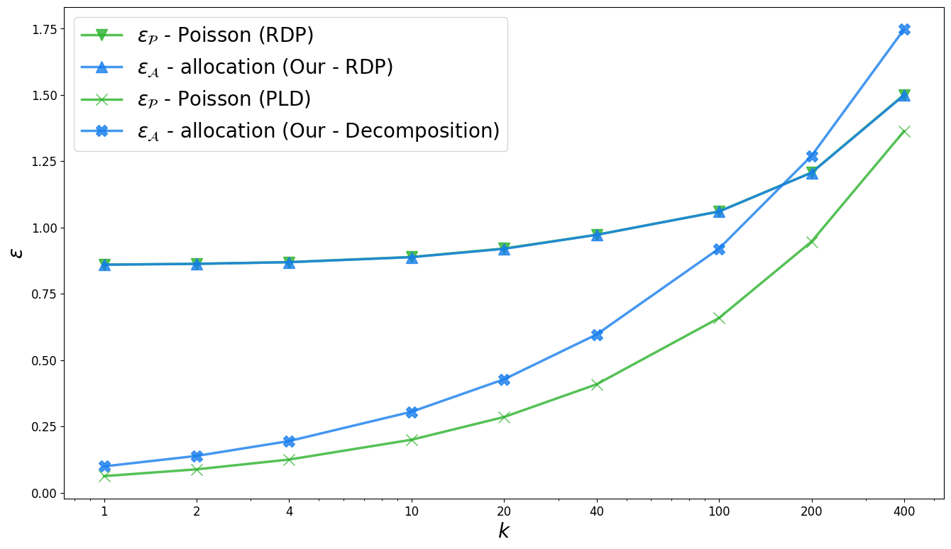
Figure 2: Upper bounds on privacy parameter $\epsilon$ for various schemes all using the Gaussian mechanism, as a function of $k$ the number of times the scheme was sequentially computed, for fixed parameters $\sigma=1$, $\delta=10^{-8}$, $t=10^{4}$. In the Poisson scheme $\lambda=1/t$. The analytic bound was omitted, since it is dominated by the decomposition method in this regime.

Since we have an exact expression for the Rényi divergence of the Gaussian mechanism, this immediately implies that

Corollary 4.7.

Given $\alpha\in\mathbb{N}$ s.t. $1<\alpha\leq t$; $\sigma>0$, and a Gaussian mechanism $N_{\sigma}$ with noise scale $\sigma$,

$$\boldsymbol{R}_{\alpha}\left(\mathcal{A}_{t}\left(N_{\sigma};1\right)\|N_{\sigma}^{t}(0)\right)=-\frac{\alpha}{\alpha-1}\left(\frac{1}{2\sigma^{2}}+\ln(t)\right)+\frac{1}{\alpha-1}\ln\left(\sum_{P\in\boldsymbol{P}(\alpha)}\binom{t}{P}e^{\sum_{p\in P}\frac{p^{2}}{2\sigma^{2}}}\right).$$

Corollary 4.7 gives an simple way to exactly compute integer RDP parameters of random allocation with Gaussian noise. Interestingly, they closely match RDP parameters of the Poisson scheme with rate $1/t$ in most regimes (e.g. Fig. 2). In fact, in some (primarily large $\epsilon$) parameter regimes the bounds based on RDP of allocation are lower than the shart PLD-based bounds for Poisson subsampling (Fig. 3). We also note that $|\boldsymbol{P}(\alpha)|$ is sub-exponential in $\alpha$, but since the typical value of $\alpha$ used for accounting is in the low tens, this quantity can be efficiently computed using several technical improvements which we discuss in Appendix B. Finally, we remark that RDP based bounds are particularly convenient for subsequent composition which necessary to obtain bounds for $k>1$ (or multi-epoch training algorithms).

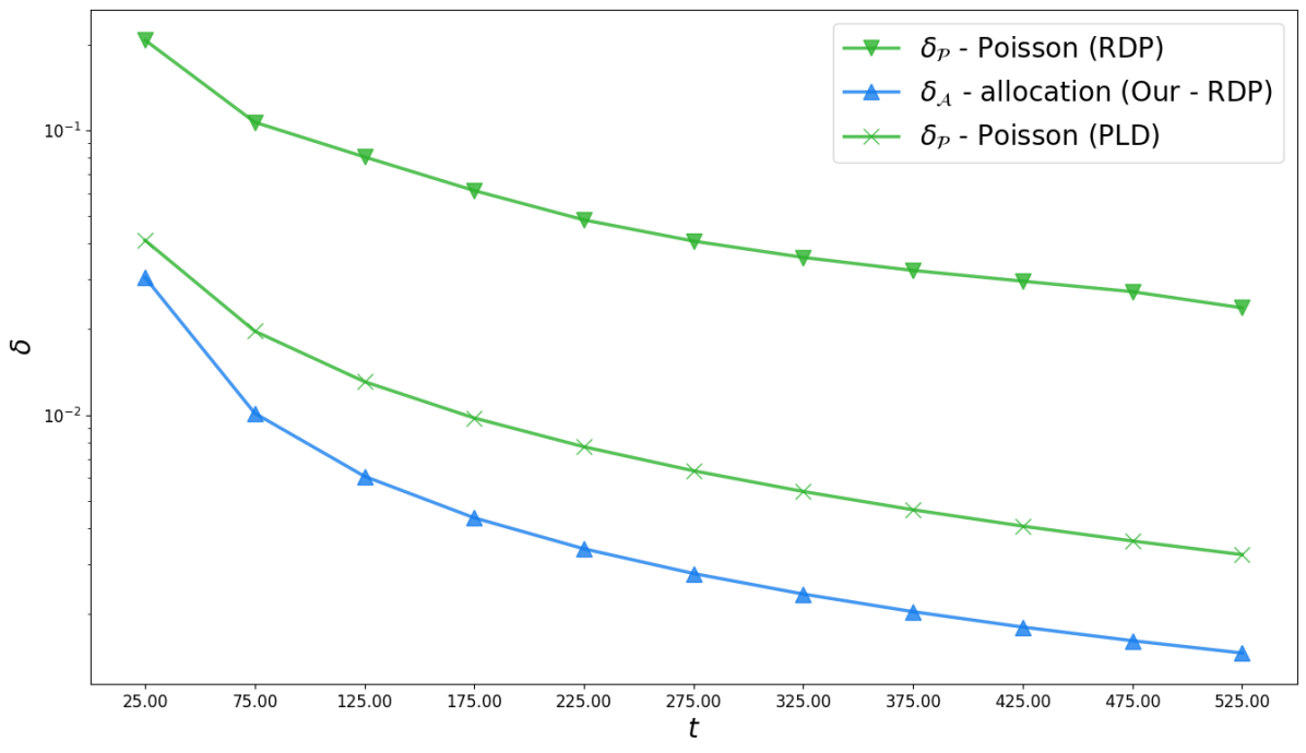
Figure 3: Upper bounds on privacy profile $\delta$ as a function of the number of steps $t$ for the Poisson and random allocation schemes. $\sigma=0.3,\epsilon=10,k=1$.

5 Discussion

Our results give the first nearly-tight and provable bounds on privacy amplification of random allocation with Gaussian noise, notably showing that they nearly match bounds known for Poisson subsampling. Together with the results of Chua et al. (2024a), our results imply that random allocation (or balls-and-bins sampling) has the utility benefits of shuffling while having the privacy benefits of Poisson subsampling. This provides a (reasonably) practical way to reconcile a long-standing and concerning discrepancy between the practical implementations of DP-SGD and its commonly-used privacy analyses.

Acknowledgments

We are grateful to Kunal Talwar for proposing the problem that we investigate here as well as suggesting the decomposition-based approach for the analysis of this problem (established in Theorem 4.1). We also thank Hilal Asi, Hannah Keller, Guy Rothblum and Katrina Ligett for thoughtful comments and motivating discussions of these results. Shenfeld’s work was supported by the Apple Scholars in AI/ML PhD Fellowship.

Appendix A Missing proofs from Section 3

A.1 Single element bound

Proof of Lemma 3.4.

We notice that for all $j\in[t-1]$ and $\boldsymbol{v}^{j}\in\mathcal{O}^{j}$,

$$P_{\mathcal{A}_{t,k}\left(M\right)}(\boldsymbol{v}^{j+1}|x,\boldsymbol{v}^{j}) =\frac{P_{\mathcal{A}_{t,k}\left(M\right)}(\boldsymbol{v}^{j+1}|x)}{P_{\mathcal{A}_{t,k}\left(M\right)}(\boldsymbol{v}^{j}|x)}$$

$$\overset{(1)}{=}\frac{\underset{\boldsymbol{i}\subseteq[t],|\boldsymbol{i}|=k}{\sum}P_{\mathcal{A}_{t,k}\left(M\right)}(\boldsymbol{v}^{j+1},\boldsymbol{I}=\boldsymbol{i}|x)}{P_{\mathcal{A}_{t,k}\left(M\right)}(\boldsymbol{v}^{j}|x)}$$

$$\overset{(2)}{=}\frac{\underset{\boldsymbol{i}\subseteq[t],|\boldsymbol{i}|=k}{\sum}P_{\mathcal{A}_{t,k}\left(M\right)}(\boldsymbol{v}^{j},\boldsymbol{I}=\boldsymbol{i}|x)\cdot P_{\mathcal{A}_{t,k}\left(M\right)}(o_{j+1}|x,\boldsymbol{I}=\boldsymbol{i},\boldsymbol{v}^{j})}{P_{\mathcal{A}_{t,k}\left(M\right)}(\boldsymbol{v}^{j}|x)}$$

$$\overset{(3)}{=}\left(\underset{\boldsymbol{i}\subseteq[t],|\boldsymbol{i}|=k,j+1\notin\boldsymbol{i}}{\sum}\frac{P_{\mathcal{A}_{t,k}\left(M\right)}(\boldsymbol{v}^{j},\boldsymbol{I}=\boldsymbol{i}|x)}{P_{\mathcal{A}_{t,k}\left(M\right)}(\boldsymbol{v}^{j}|x)}\right)P_{M}(o_{j+1}|\bot,\boldsymbol{v}^{j})$$

$$~~~~+\left(\underset{\boldsymbol{i}\subseteq[t],|\boldsymbol{i}|=k,j+1\in\boldsymbol{i}}{\sum}\frac{P_{\mathcal{A}_{t,k}\left(M\right)}(\boldsymbol{v}^{j},\boldsymbol{I}=\boldsymbol{i}|x)}{P_{\mathcal{A}_{t,k}\left(M\right)}(\boldsymbol{v}^{j}|x)}\right)P_{M}(o_{j+1}|\bot,\boldsymbol{v}^{j})$$

$$=P_{\mathcal{A}_{t,k}\left(M\right)}(j+1\notin\boldsymbol{I}|x,\boldsymbol{v}^{j})P_{M}(o_{j+1}|\bot,\boldsymbol{v}^{j})+P_{\mathcal{A}_{t,k}\left(M\right)}(j+1\in\boldsymbol{I}|x,\boldsymbol{v}^{j})P_{M}(o_{j+1}|x,\boldsymbol{v}^{j})$$

$$=(1-\lambda_{\boldsymbol{v}^{j},k,x})P_{M}(o_{j+1}|\bot,\boldsymbol{v}^{j})+\lambda_{\boldsymbol{v}^{j},k,x}P_{M}(o_{j+1}|x,\boldsymbol{v}^{j})$$

$$\overset{(3)}{=}P_{\mathcal{T}_{t,k}\left(M\right)}(\boldsymbol{v}^{j+1}|x,\boldsymbol{v}^{j}),$$

where (1) denotes the subset of steps selected by the allocation scheme by $\boldsymbol{I}$ so $\boldsymbol{I}=\boldsymbol{i}$ denotes the selected subset was $\boldsymbol{i}$, (2) results from the definition $\boldsymbol{v}^{j+1}=(o_{j+1},\boldsymbol{v}^{j})$ and Bayes law, (3) from the fact that if $j+1\in\boldsymbol{I}$ then $o_{j+1}$ depends only on a $x$ and if $j+1\notin\boldsymbol{I}$ then $o_{j+1}$ depends only on a $\bot$, and (4) is a direct result of the posterior scheme definition.

Since $P(\boldsymbol{v}|x)=\prod_{i\in[t-1]}P(\boldsymbol{v}^{j+1}|x,\boldsymbol{v}^{j})$ for any scheme, this completes the proof.

By Lemma 3.1, $\bar{\delta}_{\mathcal{A}_{t,k}\left(R\right)}(\epsilon)$ is achieved by a pair of datasets of size $1$, which proves the second part. ∎

Proof of Lemma 3.6.

For any $\mathcal{C}\subseteq\mathcal{O}^{t}$ we have

$$\underset{\boldsymbol{V}\sim\mathcal{T}_{t,k}\left(R;*\right)}{\mathbb{P}} (\boldsymbol{V}\in\mathcal{C})$$

$$=\underset{\boldsymbol{V}\sim\mathcal{T}_{t,k}\left(R;*\right)}{\mathbb{P}}(\boldsymbol{V}\in\mathcal{C}/\mathcal{B}_{\eta}^{t,k})+\underset{\boldsymbol{V}\sim\mathcal{T}_{t,k}\left(R;*\right)}{\mathbb{P}}(\boldsymbol{V}\in\mathcal{C}\cap\mathcal{B}_{\eta}^{t,k})$$

$$\overset{(1)}{=}\underset{\boldsymbol{V}\sim\mathcal{T}_{t,k,\eta}\left(R;*\right)}{\mathbb{P}}(\boldsymbol{V}\in\mathcal{C}/\mathcal{B}_{\eta}^{t,k})+\underset{\boldsymbol{V}\sim\mathcal{T}_{t,k}\left(R;*\right)}{\mathbb{P}}(\boldsymbol{V}\in\mathcal{B}_{\eta}^{t,k})$$

$$\overset{(2)}{\leq}e^{\epsilon}\underset{\boldsymbol{V}\sim R^{t}(\bot)}{\mathbb{P}}(\boldsymbol{V}\in\mathcal{C}/\mathcal{B}_{\eta}^{t,k})+\boldsymbol{H}_{e^{\epsilon}}(\mathcal{T}_{t,k,\eta}\left(R;*\right)\|R^{t}(\bot))+\underset{\boldsymbol{V}\sim\mathcal{T}_{t,k}\left(R;*\right)}{\mathbb{P}}(\boldsymbol{V}\in\mathcal{B}_{\eta}^{t,k})$$

$$\overset{(1)}{=}e^{\epsilon}\underset{\boldsymbol{V}\sim R^{t}(\bot)}{\mathbb{P}}(\boldsymbol{V}\in\mathcal{C}/\mathcal{B}_{\eta}^{t,k})+\boldsymbol{H}_{e^{\epsilon}}(\mathcal{T}_{t,k,\eta}\left(R;*\right)\|R^{t}(\bot))+\underset{\boldsymbol{V}\sim\mathcal{T}_{t,k}\left(R;*\right)}{\mathbb{P}}(\boldsymbol{V}\in\mathcal{B}_{\eta}^{t,k}),$$

$$\leq e^{\epsilon}\underset{\boldsymbol{V}\sim R^{t}(\bot)}{\mathbb{P}}(\boldsymbol{V}\in\mathcal{C})+\boldsymbol{H}_{e^{\epsilon}}(\mathcal{T}_{t,k,\eta}\left(R;*\right)\|R^{t}(\bot))+\underset{\boldsymbol{V}\sim\mathcal{T}_{t,k}\left(R;*\right)}{\mathbb{P}}(\boldsymbol{V}\in\mathcal{B}_{\eta}^{t,k}),$$

which implies

$$\delta_{\mathcal{T}_{t,k}\left(R\right)}(\epsilon) =\boldsymbol{H}_{e^{\epsilon}}(\mathcal{T}_{t,k}\left(R;*\right)\|R^{t}(\bot))$$

$$\overset{(2)}{=}\underset{\mathcal{C}\subseteq\mathcal{O}^{t}}{\sup}\left(\underset{\boldsymbol{V}\sim\mathcal{T}_{t,k}\left(R;*\right)}{\mathbb{P}}(\boldsymbol{V}\in\mathcal{C})-e^{\epsilon}\underset{\boldsymbol{V}\sim R^{t}(\bot)}{\mathbb{P}}(\boldsymbol{V}\in\mathcal{C})\right)$$

$$\leq\boldsymbol{H}_{e^{\epsilon}}(\mathcal{T}_{t,k,\eta}\left(R;*\right)\|R^{t}(\bot))+\underset{\boldsymbol{V}\sim\mathcal{T}_{t,k}\left(R;*\right)}{\mathbb{P}}(\boldsymbol{V}\in\mathcal{B}_{\eta}^{t,k})$$

$$=\delta_{\mathcal{T}_{t,k,\eta}\left(R\right)}(\epsilon)+\beta_{\mathcal{A}_{t,k}\left(R\right)}(\eta)$$

where (1) results from the definition of the truncated posterior scheme and (2) from the fact that for any couple of distributions $P,Q$ over some domain $\mathcal{O}$

$$\boldsymbol{H}_{e^{\epsilon}}(P\|Q)=\underset{\mathcal{C}\subseteq\mathcal{O}^{t}}{\sup}\left(\underset{O\sim P}{\mathbb{P}}(O\in\mathcal{C})-e^{\epsilon}\underset{O\sim Q}{\mathbb{P}}(O\in\mathcal{C})\right).$$

∎

Proof of Lemma 3.7.

We first notice that the the hockey-stick divergence of a mixture mechanism is monotonically increasing in its mixture parameter. For any $0\leq\lambda\leq\lambda^{\prime}\leq 1$ and two distributions $P_{0},P_{1}$ over some domain, denoting $Q_{\lambda}\coloneqq(1-\lambda)P_{0}+\lambda P_{1}$ we have, $Q_{\lambda^{\prime}}=\frac{1-\lambda^{\prime}}{1-\lambda}Q_{\lambda}+\frac{\lambda^{\prime}-\lambda}{1-\lambda}Q$. From the convexity of the hockey-stick divergence, for any $\alpha\geq 1$ we have

$$\boldsymbol{H}_{\alpha}(Q_{\lambda^{\prime}}\|Q)=\boldsymbol{H}_{\alpha}\left(\frac{1-\lambda^{\prime}}{1-\lambda}Q_{\lambda}+\frac{\lambda^{\prime}-\lambda}{1-\lambda}Q\|Q\right)\leq\frac{1-\lambda^{\prime}}{1-\lambda}\boldsymbol{H}_{\alpha}\left(Q_{\lambda}\|Q\right)\leq\boldsymbol{H}_{\alpha}\left(Q_{\lambda}\|Q\right).$$

Using this fact we get that the privacy profile of a single call to a Poisson subsampling mechanism is monotonically increasing in its sampling probability, so the privacy profile of every step of $\mathcal{T}_{t,k,\eta}\left(R\right)$ is upper bounded by that of $\mathcal{P}_{1,\eta}\left(R\right)$, and from Theorem 10 of Zhu et al. (2022) its $t$ times composition is the dominating pair of $\mathcal{P}_{t,\eta}\left(R\right)$, which completes the proof. ∎

Proof of Lemma 3.8.

From Lemma 3.7 in (Feldman et al., 2021), there exists a randomizer $\hat{R}$ which is $\epsilon_{0}$-DP, and for any element $x\in\mathcal{X}$ and view $\boldsymbol{v}\in\mathcal{O}^{*}$ we have $D_{TV}(R(x,\boldsymbol{v})\|\hat{R}(x,\boldsymbol{v}))\leq\delta_{0}$.

For any $i\in[t]$ consider the posterior scheme $\mathcal{T}_{t,k,(i)}\left(\hat{R}\right)$ which $\forall j<i$ returns

$$o_{j+1}\sim\left(\lambda_{\boldsymbol{v}^{j},k,*}\cdot R(*)+(1-\lambda_{\boldsymbol{v}^{j},k,*})\cdot R(\bot)\right),$$

and $\forall j\geq i$ returns

$$o_{j+1}\sim\left(\lambda_{\boldsymbol{v}^{i},k,*}\cdot\hat{R}(*)+(1-\lambda_{\boldsymbol{v}^{j},k,*})\cdot\hat{R}(\bot)\right).$$

Notice that $\mathcal{T}_{t,k,(0)}\left(\hat{R}\right)=\mathcal{T}_{t,k}\left(R\right)$ and $\mathcal{T}_{t,k,(t)}\left(\hat{R}\right)=\mathcal{T}_{t,k}\left(\hat{R}\right)$. From the definition, for any $i\in[t]$ we have $D_{TV}\left(\mathcal{T}_{t,k,(i-1)}\left(\hat{R};*\right)\|\mathcal{T}_{t,k,(i)}\left(\hat{R};*\right)\right)\leq\delta_{0}$, which implies $D_{TV}\left(\mathcal{T}_{t,k}\left(R;*\right)\|\mathcal{T}_{t,k}\left(\hat{R};*\right)\right)\leq t\delta_{0}$.

Combining this inequality with the fact that for any two distributions $P,Q$ over domain $\Omega$ and a subset $\mathcal{C}\subseteq\Omega$ we have $P(\mathcal{C})\leq Q(\mathcal{C})+D_{TV}(P\|Q)$ completes the proof. ∎

The proof of Lemma 3.9 is based on an explicit description of $\lambda_{\boldsymbol{v}^{i},x}$ in terms of the induced privacy loss.

claim A.1.

Given $i\in[t-1]$, an element $x\in\mathcal{X}$ and a view $\boldsymbol{v}^{i}\in\mathcal{O}^{i}$, we have

$$\lambda_{\boldsymbol{v}^{i},x}=\frac{1}{t+\sum_{k\in[i]}(e^{\ell(o_{k};x,\bot,\boldsymbol{v}^{k-1})}-1)}$$

Proof.

$$\lambda_{\boldsymbol{v}^{i},x} =P_{\mathcal{A}_{t}\left(M\right)}\left(I=i+1|x,\boldsymbol{v}^{i}\right)$$

$$=\frac{P_{\mathcal{A}_{t}\left(M\right)}\left(\boldsymbol{v}^{i}|x,I=i+1\right)P\left(I=i+1\right)}{P_{\mathcal{A}_{t}\left(M\right)}\left(\boldsymbol{v}^{i}|x\right)}$$

$$=\frac{\frac{1}{t}P_{\mathcal{A}_{t}\left(M\right)}\left(\boldsymbol{v}^{i}|x,I=i+1\right)}{\frac{1}{t}\sum_{k\in[t]}P_{\mathcal{A}_{t}\left(M\right)}\left(\boldsymbol{v}^{i}|x,\boldsymbol{I}=\boldsymbol{i}\right)}$$

$$=\frac{1}{\sum_{k\in[t]}\frac{P_{\mathcal{A}_{t}\left(M\right)}\left(\boldsymbol{v}^{i}|x,\boldsymbol{I}=\boldsymbol{i}\right)}{P_{\mathcal{A}_{t}\left(M\right)}\left(\boldsymbol{v}^{i}|x,I=i+1\right)}}$$

$$=\frac{1}{t-i+\sum_{k\in[i]}\frac{P_{M}\left(o_{k}|x,\boldsymbol{v}^{k-1}\right)}{P_{M}\left(o_{k}|\bot,\boldsymbol{v}^{k-1}\right)}}$$

$$=\frac{1}{t+\sum_{k\in[i]}(e^{\ell(o_{k};x,\bot,\boldsymbol{v}^{k-1})}-1)}$$

∎

Proof of Lemma 3.9.

First notice that,

$$\underset{\boldsymbol{V}\sim\mathcal{A}_{t}\left(M;x\right)}{\mathbb{P}}\left(\lambda_{\boldsymbol{V},x}>\eta\right)=\frac{1}{t}\sum_{i\in[t]}\underset{\boldsymbol{V}\sim\mathcal{A}_{t}\left(M;x\right)}{\mathbb{P}}\left(\lambda_{\boldsymbol{V},x}>\eta~|~I=i\right),$$

and for any $i\in[t]$,

$$\underset{\boldsymbol{V}\sim\mathcal{A}_{t}\left(M;x\right)}{\mathbb{P}} \left(\lambda_{\boldsymbol{V},x}>\eta~|~I=i\right)$$

$$=\underset{\boldsymbol{V}\sim\mathcal{A}_{t}\left(M;x\right)}{\mathbb{P}}\left(\underset{k\in[t-1]}{\max}\left(\frac{1}{t+\sum_{j\in[k]}(e^{\ell(o_{j};x,\bot,\boldsymbol{v}^{j-1})}-1)}\right)>\frac{1}{t(1+\gamma)}~|~I=i\right)$$

$$=\underset{\boldsymbol{V}\sim\mathcal{A}_{t}\left(M;x\right)}{\mathbb{P}}\left(\underset{k\in[t-1]}{\max}\left(\sum_{j\in[k]}(1-e^{\ell(o_{j};x,\bot,\boldsymbol{v}^{j-1})})\right)>\gamma t~|~I=i\right)$$

We can now define the following martingale; $D_{0}\coloneqq 0$, $\forall k\in[t]:D_{k}\coloneqq 1-e^{\ell(O_{k};x,\bot,\boldsymbol{v}^{k-1})}$, and $Y_{i}\coloneqq\sum_{j=0}^{i}D_{j}$. Notice that this is a sub-martingale since for any $i\in[n-1]$

$$\underset{O\sim M(\bot,\boldsymbol{v}^{i})}{\mathbb{E}}\left[1-e^{\ell(O;x,\bot,\boldsymbol{v}^{i})}\right]=1-\underset{O\sim M(\bot,\boldsymbol{v})}{\mathbb{E}}\left[\frac{P_{M}(O|x,\boldsymbol{v}^{i})}{P_{M}(O|\bot,\boldsymbol{v}^{i})}\right]=0$$

and

$$\underset{O\sim M(x,\boldsymbol{v}^{i})}{\mathbb{E}}\left[1-e^{\ell(O;x,\bot,\boldsymbol{v}^{i})}\right]=1-\exp\left(\boldsymbol{R}_{2}\left(M(x,\boldsymbol{v}^{i})\|M(\bot,\boldsymbol{v}^{i})\right)\right)\leq 0,$$

where $\boldsymbol{R}_{\alpha}$ is the $\alpha$-Rényi divergence.

From the fact $M$ is $\epsilon_{0}$-DP we have $1-e^{-\epsilon_{0}}\leq D_{k}\leq 1-e^{\epsilon_{0}}$ almost surely, so the range of $D_{j}$ is bounded by $e^{\epsilon_{0}}-e^{-\epsilon_{0}}=2\cosh(\epsilon_{0})$, so we can invoke the Maximal Azuma-Hoeffding inequality and get for any $i\in[t]$,

$$\underset{\boldsymbol{V}\sim\mathcal{A}_{t}\left(M;x\right)}{\mathbb{P}} \left(\lambda_{\boldsymbol{V},x}>\eta~|~I=i\right)$$

$$=\underset{\boldsymbol{V}\sim\mathcal{A}_{t}\left(M;x\right)}{\mathbb{P}}\left(\underset{k\in[t-1]}{\max}\left(\sum_{j\in[k]}(1-e^{\ell(o_{j};x,\bot,\boldsymbol{v}^{j-1})})\right)>\gamma t~|~I=i\right)$$

$$\leq\underset{\boldsymbol{V}\sim\mathcal{A}_{t,k}\left(R;\bot\right)}{\mathbb{P}}\left(\underset{k\in[t]}{\max}\left(Y_{k}\right)>\gamma t\right)$$

$$\leq\exp\left(-\frac{t\gamma^{2}}{2\cosh^{2}(\epsilon_{0})}\right)$$

∎

A.2 Multiple allocations

Proof of Corollary 3.12.

From Theorem 3.2, each of the schemes has a privacy profile $\delta_{\mathcal{A}_{t/k}\left(M\right)}(\epsilon)\leq\delta_{\mathcal{P}_{t/k,\eta}\left(R\right)}(\epsilon)+t/k\delta_{0}+\delta/k$, where $\eta\coloneqq\min\left\{\frac{k}{t(1-\gamma)},1\right\}$ and $\gamma\coloneqq\cosh(\epsilon_{0})\cdot\sqrt{\frac{2k}{t}\ln\left(\frac{k}{\delta}\right)}$. Applying the union bound to the $t/k\delta_{0}$ and $\delta/k$ terms, and using the fact that the composition of Poisson schemes is a longer Poisson scheme completes the proof. ∎

Appendix B Missing proofs from Section 4

B.1 Decomposing Poisson

Proof of Lemma 4.2.

To prove this claim, we recall the technique used in the proof of Theorem 3.2. We proved in Lemma 3.4 that $\mathcal{A}_{t,k}\left(R;x\right)$ and $\mathcal{T}_{t,k}\left(R;x\right)$ are identically distributed. From the non-adaptivity assumption, this is just a sequence of repeated calls to the mixture mechanism $\lambda_{\boldsymbol{v}^{i},k,*}\cdot R(*)+(1-\lambda_{\boldsymbol{v}^{i},k,*})\cdot R(\bot)$.

Next we recall the fact proven in Lemma 3.7 that the hockey-stick divergence between this mixture mechanism and $R(\bot)$ is monotonically increasing in $\lambda$. Since $\lambda_{\boldsymbol{v}^{i},k^{\prime},*}\geq\lambda_{\boldsymbol{v}^{i},k,*}$ for any $k^{\prime}>k$, this means the hockey-stick divergence between this mixture mechanism and $R(\bot)$ is monotonically increasing in $k$, which implies $\delta_{\mathcal{A}_{t,k}\left(R\right)}(\epsilon)\leq\delta_{\mathcal{A}_{t,k^{\prime}}\left(R\right)}(\epsilon)$ for any $\epsilon>0$, thus completing the proof of the first part.

The proof of the second part is identical, since the posterior sampling probability induced by any mixture of $\mathcal{A}_{t,k_{1}}\left(M\right),\ldots,\mathcal{A}_{t,k_{j}}\left(M\right)$ is greater than the one induced by $\mathcal{A}_{t,k}\left(M\right)$ the same reasoning follows. ∎

Lemma B.1 (Advanced joint convexity (Balle et al., 2018)).

Given $\eta\in[0,1]$; $\alpha\geq 0$ and three distribution $P_{0},P_{1},Q$ over some domain, we have

$$\boldsymbol{H}_{\alpha}((1-\eta)Q+\eta P_{0}\|(1-\eta)Q+\eta P_{1})=\eta\boldsymbol{H}_{\alpha^{\prime}}(P_{0}\|(1-\eta^{\prime})Q+\eta^{\prime}P_{1}),$$

where $\alpha^{\prime}\coloneqq 1+(\alpha-1)/\eta$ and $\eta^{\prime}\coloneqq\alpha/\alpha^{\prime}$.

Proof of Lemma 4.4.

First notice that,

$$\mathcal{P}_{t,\lambda}\left(R;x\right) \overset{(1)}{=}\sum_{k=0}^{t}B_{t,\lambda}(k)\cdot\mathcal{A}_{t,k}\left(R;x\right)$$

$$=B_{t,\lambda}(0)\cdot\mathcal{A}_{t,0}\left(R;x\right)+\sum_{k\in[t]}B_{t,\lambda}(k)\cdot\mathcal{A}_{t,k}\left(R;x\right)$$

$$\overset{(2)}{=}\left(1-\lambda\right)^{t}\cdot\mathcal{A}_{t,0}\left(R;x\right)+\lambda^{\prime}\cdot\mathcal{P}_{t,\lambda}^{+}(R;x)$$

$$\overset{(3)}{=}(1-\lambda^{\prime})\cdot R^{t}(\bot)+\lambda^{\prime}\cdot\mathcal{P}_{t,\lambda}^{+}(R;x),$$

where (1) results from Lemma 4.3, (2) from the definition of the binomial distribution, $\lambda^{\prime}$ and $\mathcal{P}_{t,\lambda}^{+}(R)$, and (3) from the definition of $\lambda^{\prime}$ and the fact $\mathcal{A}_{t,0}\left(M;x\right)=R^{t}(\bot)$.

From Lemma B.1 we have,

$$\boldsymbol{H}_{\alpha}(\mathcal{P}_{t,\lambda}\left(R;x\right)\|\mathcal{P}_{t,\lambda}\left(R;\bot\right))=\boldsymbol{H}_{\alpha}((1-\lambda^{\prime})R^{t}(\bot)+\lambda^{\prime}\mathcal{P}_{t,\lambda}^{+}(R;x)\|R^{t}(\bot))=\lambda^{\prime}\boldsymbol{H}_{1+(\alpha-1)/\lambda^{\prime}}(\mathcal{P}_{t,\lambda}^{+}(R;x)\|R^{t}(\bot)).$$

Setting $1+(\alpha-1)/\lambda^{\prime}=e^{\epsilon}$ and inverting the equation we get,

$$\boldsymbol{H}_{e^{\epsilon}}(\mathcal{P}_{t,\lambda}^{+}(R;x)\|R^{t}(\bot))=\frac{1}{\lambda^{\prime}}\boldsymbol{H}_{\alpha}(\mathcal{P}_{t,\lambda}\left(R;x\right)\|\mathcal{P}_{t,\lambda}\left(R;\bot\right))=\frac{1}{\lambda^{\prime}}\boldsymbol{H}_{e^{\epsilon^{\prime}}}(\mathcal{P}_{t,\lambda}\left(R;x\right)\|\mathcal{P}_{t,\lambda}\left(R;\bot\right)),$$

which completes the proof ∎

Proof of Corollary 4.5.

Notice that,

$$\delta_{\mathcal{P}_{t,\lambda,k}\left(M\right)}(\epsilon) \overset{(1)}{\leq}\delta_{\mathcal{P}_{t,\lambda,k}\left(R\right)}(\epsilon)$$

$$=\boldsymbol{H}_{e^{\epsilon}}\left(\mathcal{P}_{t,\lambda,k}\left(R;*\right)\|\mathcal{P}_{t,\lambda,k}\left(R;\bot\right)\right)$$

$$\overset{(2)}{=}\boldsymbol{H}_{e^{\epsilon}}\left(\left(\sum_{i=0}^{k-1}B_{t,\lambda}(i)\mathcal{A}_{t,i}\left(R;*\right)\right)+\left(\sum_{i=k}^{t}B_{t,\lambda}(i)\right)\mathcal{A}_{t,k}\left(R;*\right)\|R^{t}(\bot)\right)$$

$$\overset{(3)}{\leq}\boldsymbol{H}_{e^{\epsilon}}\left(\sum_{i=0}^{t}B_{t,\lambda}(i)\mathcal{A}_{t,i}\left(R;*\right)\|R^{t}(\bot)\right)$$

$$=\delta_{\mathcal{P}_{t,\lambda}\left(M\right)}(\epsilon),$$

where (1) results from Lemma 3.1, (2) from Lemma 4.3 and the definition of $\mathcal{P}_{t,\lambda,k}\left(R\right)$, and (3) from Lemma 4.2. ∎

B.2 RDP bound

Proof of Theorem 4.6.

From the definition,

$$\boldsymbol{D}_{\alpha}\left(\mathcal{A}_{t}\left(R;*\right)\|R^{t}(\bot)\right) =\underset{\boldsymbol{V}\sim R^{t}(\bot)}{\mathbb{E}}\left[\left(\frac{P_{\mathcal{A}_{t}\left(R\right)}(\boldsymbol{V}|*)}{P_{\mathcal{A}_{t}\left(R\right)}(\boldsymbol{V}|\bot)}\right)^{\alpha}\right]$$

$$\overset{(1)}{=}\underset{\boldsymbol{V}\sim R^{t}(\bot)}{\mathbb{E}}\left[\left(\frac{1}{t}\sum_{i\in[t]}\frac{P_{R}(O_{i}|*)}{P_{R}(O_{i}|\bot)}\right)^{\alpha}\right]$$

$$=\frac{1}{t^{\alpha}}\sum_{i_{1},\ldots,i_{\alpha}\in[t]}\underset{\boldsymbol{V}\sim R^{t}(\bot)}{\mathbb{E}}\left[\prod_{k\in[\alpha]}\frac{P_{R}(O_{i_{k}}|*)}{P_{R}(O_{i_{k}}|\bot)}\right]$$

$$\overset{(2)}{=}\frac{1}{t^{\alpha}}\sum_{P\in\boldsymbol{P}(\alpha)}\binom{t}{P}\prod_{p\in P}\underset{O\sim R(\bot)}{\mathbb{E}}\left[\left(\frac{P_{R}(O|*)}{P_{R}(O|\bot)}\right)^{p}\right]$$

$$=\frac{1}{t^{\alpha}}\sum_{P\in\boldsymbol{P}(\alpha)}\binom{t}{P}\prod_{p\in P}\boldsymbol{D}_{p}\left(R(*)\|R(\bot)\right),$$

where (1) results from the identity of the dominating pair, and (2) from the fact $O_{i}$ and $O_{j}$ are independent for any $i\neq j$. ∎

Proof of Corollary 4.7.

From the definition of the Rényi divergence for the Gaussian mechanism,

$$\boldsymbol{R}_{\alpha}\left(\mathcal{A}_{t}\left(N_{\sigma};1\right)\|N_{\sigma}^{t}(0)\right) =\frac{1}{\alpha-1}\ln\left(\boldsymbol{D}_{\alpha}\left(\mathcal{A}_{t}\left(N_{\sigma};1\right)\|N_{\sigma}^{t}(0)\right)\right)$$

$$=\frac{1}{\alpha-1}\ln\left(\frac{1}{t^{\alpha}}\sum_{P\in\boldsymbol{P}(\alpha)}\binom{t}{P}\prod_{p\in P}\boldsymbol{D}_{p}\left(N_{\sigma}(1)\|N_{\sigma}(0)\right)\right)$$

$$=\frac{1}{\alpha-1}\ln\left(\frac{1}{t^{\alpha}}\sum_{P\in\boldsymbol{P}(\alpha)}\binom{t}{P}\prod_{p\in P}e^{\frac{p(p-1)}{2\sigma^{2}}}\right)$$

$$=\frac{1}{\alpha-1}\ln\left(\frac{e^{-\frac{\alpha}{2\sigma^{2}}}}{t^{\alpha}}\sum_{P\in\boldsymbol{P}(\alpha)}\binom{t}{P}e^{\sum_{p\in P}\frac{p^{2}}{2\sigma^{2}}}\right)$$

$$=-\frac{\alpha}{2(\alpha-1)\sigma^{2}}-\frac{\alpha}{\alpha-1}\ln\left(t\right)+\frac{1}{\alpha-1}\ln\left(\sum_{P\in\boldsymbol{P}(\alpha)}\binom{t}{P}e^{\sum_{p\in P}\frac{p^{2}}{2\sigma^{2}}}\right).$$

∎

We remark that the expression in Corollary 4.7 was previously computed in Liew & Takahashi (2022). In this (unpublished) work the authors give an incorrect proof that datasets $(0,\ldots,0,1)$ and $(0,\ldots,0)$ are a dominating pair of datasets for the shuffle scheme applied to Gaussian mechanism. Their analysis of the RDP bound for this pair of distributions is correct (even if significantly longer) and the final expression is identical to ours.

Appendix C Implementation details

Computation time of the naive implementation of our RDP calculation ranges between second and minutes on a typical personal computer, depending on the $\alpha$ value and other parameters, but can be improved by several orders of magnitude using several programming and analytic steps which we briefly discuss here.

On the programming side, we used vectorization and hashing to reduce runtime. To avoid overflow we computed most quantities in log form, and used and the LSE trick. While significantly reducing the runtime, programming improvements cannot escape the inevitable exponential (in $alpha$) nature of this method. Luckily, in most settings, $\alpha^{*}$ - the $\alpha$ value which induces the tightest bound on $\epsilon$ is typically in the low $10$s. Unfortunately, finding $\alpha^{*}$ requires computing $\boldsymbol{R}_{\alpha}$, so reducing the range of $\alpha$ values for which $\boldsymbol{R}_{\alpha}$ is crucial.

We do so by proving an upper bound on $\alpha^{*}$ in terms of a known bound on $\epsilon$.

claim C.1.

Given $\delta\in(0,1)$ and two distributions $P,Q$ and, denote by $\varepsilon(\delta)\coloneqq\underset{x>0}{\inf}(\delta(x)<\delta)$. Given $\epsilon>0$, if $\varepsilon(\delta)\leq\epsilon$ and $\boldsymbol{R}_{\alpha}\left(P\|Q\right)>\epsilon$, then $\alpha^{*}<\alpha$.

I direct implication of this Lemma is that searching on monotonically increasing values of $\alpha$ and using the best bound on $\epsilon$ achieved at any point to check the relevancy of $\alpha$, we don’t have to compute many values of $\alpha$ greater than $\alpha^{*}$ before we stop.

Proof.

Denote by $\gamma_{\delta}(\alpha)$ the bound on $\epsilon$ achieved using $\boldsymbol{R}_{\alpha}\left(P\|Q\right)$. From Proposition 12 in Canonne et al. (2020), $\gamma_{\delta}(\alpha)=\boldsymbol{R}_{\alpha}\left(P\|Q\right)+\phi(\alpha)$ for a non negative $\phi$ (except for the range $\alpha>1/(2\delta)$ which provides a vacuous bound). Since $\boldsymbol{R}_{\alpha}\left(P\|Q\right)$ is monotonically non-decreasing in $\alpha$ we have for any $\alpha^{\prime}\geq\alpha$,

$$\gamma_{\delta}(\alpha^{\prime})\geq\boldsymbol{R}_{\alpha^{\prime}}\left(P\|Q\right)\geq\boldsymbol{R}_{\alpha}\left(P\|Q\right)\geq\epsilon,$$

so it cannot provide a better bound on $\alpha$. ∎

Appendix D Direct analysis and simulation

For completeness, we state how one can directly estimate the hockey-stick divergence of the entire random allocation scheme. This technique was first presented in the context of the Gaussian mechanism by Chua et al. (2024a).

We first provide an exact expression for the privacy profile of the random allocation scheme.

Lemma D.1.

For any randomizer $R$ and $\epsilon>0$ we have,

$$\delta_{\mathcal{A}_{t}\left(R\right)}(\epsilon)=\underset{\boldsymbol{V}\sim R^{t}(\bot)}{\mathbb{E}}\left[\left[\frac{1}{t}\sum_{i\in[t]}e^{\ell(O_{i};*,\bot)}-e^{\epsilon}\right]_{+}\right],$$

where $R^{t}(\bot)$ denotes $t$ repeated calls to $R(\bot)$.

Given $\sigma>0$, if $N_{\sigma}$ is a Gaussian mechanism with noise scale $\sigma$ we have,

$$\delta_{\mathcal{A}_{t}\left(N_{\sigma}\right)}(\epsilon)=\underset{\boldsymbol{Z}\sim\mathcal{N}(\bar{0},\sigma^{2}I_{t})}{\mathbb{E}}\left[\left[\frac{1}{t}\sum_{i\in[t]}e^{\frac{2Z_{i}-1}{2\sigma^{2}}}-e^{\epsilon}\right]_{+}\right]$$

This quantity can be directly estimated using Monte Carlo simulation, and Chua et al. (2024a) proposed several improved sampling methods in terms of run-time and stability.

We note that up to simple algebraic manipulations, this hockey-stick divergence is essentially the expectation of the right tail of the sum of $t$ independent log-normal random variables, which can be approximated as a single log-normal random variable (Neelesh B. et al., 2007), but this approximation typically provide useful guarantees only for large number of steps. Instead, we use two different techniques to provide provable bounds for this quantity.

Proof.

Denote by $I$ the index of the selected allocation. Notice that for any $i\in[t]$ we have,

$$P_{\mathcal{A}_{t}\left(R\right)}(\boldsymbol{v}|*,I=i)=\left(\prod_{j=1}^{i-1}P_{R}(o_{j}|\bot,\boldsymbol{)}\right)P_{R}(o_{i}|*)\left(\prod_{j=1}^{i-1}P_{R}(o_{j}|\bot)\right)=P_{\mathcal{A}_{t}\left(R\right)}(\boldsymbol{v}|\bot)\cdot\frac{P_{R}(o_{i}|*)}{P_{R}(o_{i}|\bot)}$$

$$\Rightarrow P_{\mathcal{A}_{t}\left(R\right)}(\boldsymbol{v}|*)=\frac{1}{t}\sum_{i\in[t]}P_{\mathcal{A}_{t}\left(R\right)}(\boldsymbol{v}|*,I=i)=\frac{1}{t}P_{\mathcal{A}_{t}\left(R\right)}(\boldsymbol{v}|\bot)\sum_{i\in[t]}\frac{P_{R}(o_{i}|*)}{P_{R}(o_{i}|\bot)}$$

Using this identity we get,

$$\ell(\boldsymbol{v};*,\bot)=\ln\left(\frac{P_{\mathcal{A}_{t}\left(R\right)}(\boldsymbol{v}|x)}{P_{\mathcal{A}_{t}\left(R\right)}(\boldsymbol{v}|\bot)}\right)=\ln\left(\frac{1}{t}\sum_{i\in[t]}\frac{P_{R}(o_{i}|*)}{P_{R}(o_{i}|\bot)}\right)=\ln\left(\frac{1}{t}\sum_{i\in[t]}e^{\ell(O_{i};x,\bot)}\right).$$

Plugging this into the definition of the hockey-stick divergence completes the proof of the first part.

The second part is a direct result of the fact the dominating pair of the random allocation scheme of the Gaussian mechanism is $1$ vs. $\bot$, and that in the case of the Gaussian mechanism $\ell(o;1,0)=\frac{2o_{i}-1}{2\sigma^{2}}$. ∎

References

- Abadi et al. (2016) Abadi, M., Chu, A., Goodfellow, I., McMahan, H. B., Mironov, I., Talwar, K., and Zhang, L. Deep learning with differential privacy. In Proceedings of the 2016 ACM SIGSAC conference on computer and communications security, pp. 308–318, 2016.
- Annamalai et al. (2024) Annamalai, M. S. M. S., Balle, B., De Cristofaro, E., and Hayes, J. To shuffle or not to shuffle: Auditing dp-sgd with shuffling. arXiv preprint arXiv:2411.10614, 2024.
- Balle & Wang (2018) Balle, B. and Wang, Y.-X. Improving the gaussian mechanism for differential privacy: Analytical calibration and optimal denoising. In International Conference on Machine Learning, pp. 394–403. PMLR, 2018.
- Balle et al. (2018) Balle, B., Barthe, G., and Gaboardi, M. Privacy amplification by subsampling: Tight analyses via couplings and divergences. Advances in neural information processing systems, 31, 2018.
- Balle et al. (2019) Balle, B., Bell, J., Gascón, A., and Nissim, K. The privacy blanket of the shuffle model. In Advances in Cryptology–CRYPTO 2019: 39th Annual International Cryptology Conference, Santa Barbara, CA, USA, August 18–22, 2019, Proceedings, Part II 39, pp. 638–667. Springer, 2019.
- Balle et al. (2020) Balle, B., Kairouz, P., McMahan, B., Thakkar, O., and Guha Thakurta, A. Privacy amplification via random check-ins. Advances in Neural Information Processing Systems, 33:4623–4634, 2020.
- Barthe et al. (2012) Barthe, G., Köpf, B., Olmedo, F., and Zanella Beguelin, S. Probabilistic relational reasoning for differential privacy. In Proceedings of the 39th annual ACM SIGPLAN-SIGACT symposium on Principles of programming languages, pp. 97–110, 2012.
- Bassily et al. (2014) Bassily, R., Smith, A., and Thakurta, A. Private empirical risk minimization: Efficient algorithms and tight error bounds. In 2014 IEEE 55th annual symposium on foundations of computer science, pp. 464–473. IEEE, 2014.
- Bittau et al. (2017) Bittau, A., Erlingsson, Ú., Maniatis, P., Mironov, I., Raghunathan, A., Lie, D., Rudominer, M., Kode, U., Tinnes, J., and Seefeld, B. Prochlo: Strong privacy for analytics in the crowd. In Proceedings of the 26th symposium on operating systems principles, pp. 441–459, 2017.
- Canonne et al. (2020) Canonne, C. L., Kamath, G., and Steinke, T. The discrete gaussian for differential privacy. Advances in Neural Information Processing Systems, 33:15676–15688, 2020.
- Chen et al. (2024) Chen, W.-N., Song, D., Ozgur, A., and Kairouz, P. Privacy amplification via compression: Achieving the optimal privacy-accuracy-communication trade-off in distributed mean estimation. Advances in Neural Information Processing Systems, 36, 2024.
- Cheu et al. (2019) Cheu, A., Smith, A., Ullman, J., Zeber, D., and Zhilyaev, M. Distributed differential privacy via shuffling. In Advances in Cryptology–EUROCRYPT 2019: 38th Annual International Conference on the Theory and Applications of Cryptographic Techniques, Darmstadt, Germany, May 19–23, 2019, Proceedings, Part I 38, pp. 375–403. Springer, 2019.
- Chua et al. (2024a) Chua, L., Ghazi, B., Harrison, C., Leeman, E., Kamath, P., Kumar, R., Manurangsi, P., Sinha, A., and Zhang, C. Balls-and-bins sampling for dp-sgd. arXiv preprint arXiv:2412.16802, 2024a.
- Chua et al. (2024b) Chua, L., Ghazi, B., Kamath, P., Kumar, R., Manurangsi, P., Sinha, A., and Zhang, C. How private are dp-sgd implementations? In Forty-first International Conference on Machine Learning, 2024b.
- Chua et al. (2024c) Chua, L., Ghazi, B., Kamath, P., Kumar, R., Manurangsi, P., Sinha, A., and Zhang, C. Scalable dp-sgd: Shuffling vs. poisson subsampling. arXiv preprint arXiv:2411.04205, 2024c.
- Dwork et al. (2006) Dwork, C., Kenthapadi, K., McSherry, F., Mironov, I., and Naor, M. Our data, ourselves: Privacy via distributed noise generation. In Advances in Cryptology-EUROCRYPT 2006: 24th Annual International Conference on the Theory and Applications of Cryptographic Techniques, St. Petersburg, Russia, May 28-June 1, 2006. Proceedings 25, pp. 486–503. Springer, 2006.
- Erlingsson et al. (2019) Erlingsson, Ú., Feldman, V., Mironov, I., Raghunathan, A., Talwar, K., and Thakurta, A. Amplification by shuffling: From local to central differential privacy via anonymity. In Proceedings of the Thirtieth Annual ACM-SIAM Symposium on Discrete Algorithms, pp. 2468–2479. SIAM, 2019.
- Feldman et al. (2021) Feldman, V., McMillan, A., and Talwar, K. Hiding among the clones: A simple and nearly optimal analysis of privacy amplification by shuffling. In 2021 IEEE 62nd Annual Symposium on Foundations of Computer Science (FOCS), pp. 954–964. IEEE, 2021.
- Feldman et al. (2023) Feldman, V., McMillan, A., and Talwar, K. Stronger privacy amplification by shuffling for rényi and approximate differential privacy. In Proceedings of the 2023 Annual ACM-SIAM Symposium on Discrete Algorithms (SODA), pp. 4966–4981. SIAM, 2023.
- Girgis et al. (2021) Girgis, A. M., Data, D., Diggavi, S., Kairouz, P., and Suresh, A. T. Shuffled model of federated learning: Privacy, accuracy and communication trade-offs. IEEE Journal on Selected Areas in Information Theory, 2(1):464–478, 2021. doi: 10.1109/JSAIT.2021.3056102.
- Kairouz et al. (2015) Kairouz, P., Oh, S., and Viswanath, P. The composition theorem for differential privacy. In International conference on machine learning, pp. 1376–1385. PMLR, 2015.
- Kairouz et al. (2021) Kairouz, P., McMahan, B., Song, S., Thakkar, O., Thakurta, A., and Xu, Z. Practical and private (deep) learning without sampling or shuffling. In International Conference on Machine Learning, pp. 5213–5225. PMLR, 2021.
- Kasiviswanathan et al. (2011) Kasiviswanathan, S. P., Lee, H. K., Nissim, K., Raskhodnikova, S., and Smith, A. What can we learn privately? SIAM Journal on Computing, 40(3):793–826, 2011.
- Koskela et al. (2022) Koskela, A., Heikkilä, M. A., and Honkela, A. Numerical accounting in the shuffle model of differential privacy. Transactions on Machine Learning Research, 2022.
- Lebeda et al. (2024) Lebeda, C. J., Regehr, M., Kamath, G., and Steinke, T. Avoiding pitfalls for privacy accounting of subsampled mechanisms under composition. arXiv preprint arXiv:2405.20769, 2024.
- Liew & Takahashi (2022) Liew, S. P. and Takahashi, T. Shuffle gaussian mechanism for differential privacy. arXiv preprint arXiv:2206.09569, 2022.
- Lyu (2022) Lyu, X. Composition theorems for interactive differential privacy. Advances in Neural Information Processing Systems, 35:9700–9712, 2022.
- Mironov (2017) Mironov, I. Rényi differential privacy. In 2017 IEEE 30th computer security foundations symposium (CSF), pp. 263–275. IEEE, 2017.
- Neelesh B. et al. (2007) Neelesh B., M., Jingxian, W., Andreas F., M., and Jin, Z. Approximating a sum of random variables with a lognormal. Transactions on Wireless Communications, 6(7):2690–2699, 2007.
- Steinke (2022) Steinke, T. Composition of differential privacy & privacy amplification by subsampling. arXiv preprint arXiv:2210.00597, 2022.
- Vadhan & Wang (2021) Vadhan, S. and Wang, T. Concurrent composition of differential privacy. In Theory of Cryptography: 19th International Conference, TCC 2021, Raleigh, NC, USA, November 8–11, 2021, Proceedings, Part II 19, pp. 582–604. Springer, 2021.
- Vadhan & Zhang (2023) Vadhan, S. and Zhang, W. Concurrent composition theorems for differential privacy. In Proceedings of the 55th Annual ACM Symposium on Theory of Computing, pp. 507–519, 2023.
- Zhu et al. (2022) Zhu, Y., Dong, J., and Wang, Y.-X. Optimal accounting of differential privacy via characteristic function. In International Conference on Artificial Intelligence and Statistics, pp. 4782–4817. PMLR, 2022.