Abstract

Performative prediction models account for feedback loops in decision-making processes where predictions influence future data distributions. While existing work largely assumes insensitivity of data distributions to small strategy changes, this assumption usually fails in real-world competitive (i.e. multi-agent) settings. For example, in Bertrand-type competitions, a small reduction in one firm’s price can lead that firm to capture the entire demand, while all others sharply lose all of their customers.

We study a representative setting of multi-agent performative prediction in which insensitivity assumptions do not hold, and investigate the convergence of natural dynamics. To do so, we focus on a specific game that we call the “Bank Game”, where two lenders compete over interest rates and credit score thresholds. Consumers act similarly as to in a Bertrand Competition, with each consumer selecting the firm with the lowest interest rate that they are eligible for based on the firms’ credit thresholds. Our analysis characterizes the equilibria of this game and demonstrates that when both firms use a common and natural no-regret learning dynamic—exponential weights—with proper initialization, the dynamics always converge to stable outcomes despite the general-sum structure. Notably, our setting admits multiple stable equilibria, with convergence dependent on initial conditions. We also provide theoretical convergence results in the stochastic case when the utility matrix is not fully known, but each learner can observe sufficiently many samples of consumers at each time step to estimate it, showing robustness to slight mis-specifications. Finally, we provide experimental results that validate our theoretical findings.

1 Introduction

Much of machine learning operates under the assumption of a static, independently and identically distributed (i.i.d.) data paradigm, where the data generating process remains fixed and unaffected by the predictions made by the model. However, in many high-stakes decision-making settings, predictions and decisions often induce strategic or behavioral responses as well as distributional shifts in the populations they affect. These shifts create feedback loops between predictions, decisions, and outcomes, potentially altering the statistical properties of the data and of the decisions made over time. This phenomenon is known as Performative Prediction [1].

Performative prediction arises in diverse applications. In lending, for example, credit scoring models predict the likelihood of default based on past borrower behavior, and these predictions determine whether a loan is granted and at what interest rate. Borrowers who receive higher interest rates may find it even harder to repay their loans, altering the distribution of future borrowers and their estimated likelihood of default. Further, borrowers denied loans may take actions to increase their credit score or financial responsibility, again changing the distribution of likelihood of repayment in future time steps. In multi-player settings, for example when there is competition between different mortgage companies (here, “learners”), the distribution of applicants seen by each learner can frequently further depend on decisions made by both learners—for example, an individual may choose the mortgage company they are eligible for with the lowest interest rate. In turn, how mortgage companies decide to update their lending policy in each time step is a function of their historical lending policies. Importantly, this performativity raises challenges: the dynamics we describe can lead to model instability, as predictions drive changes in behavior that, if not properly accounted for, may prevent the system from reaching a stable equilibrium.

Performative prediction and dynamic settings with distribution shifts and strategic responses in the case of a single learner have been receiving significant attention over the past few years [1, 2, 3, 4, 5, 6, 7, 8]. Here, the goal is to characterize which dynamics converge under what condition to what is called a stable model: i.e., a model such that, if we were to deploy said model and re-train it based on the responses to the current model, we would still obtain the same model—basically, even under performativity, the model will not change even in response to its induced distribution shift. [1] provides necessary and sufficient conditions for certain simple dynamics (namely, repeated empirical risk minimization and gradient descent) to converge to a unique, stable model. They also provide conditions in which this model is optimal, i.e. it minimizes the performative loss (that takes performative distribution shifts into account).

However, there has been significantly less attention paid to settings with multiple learners that may be competing against each other [9, 10]. [9] consider a setting where each learner obtains an i.i.d. sub-sample of the total population they are make prediction on, but where the fraction of the population that is assigned to them depends on all the learners’ decisions—for example, a bank or mortgage company with lower interest rates may attract more consumers. However, they do not model self-selection effects, where different types of consumers may prefer different learners depending on the learner’s decisions, in which case each learner gets a biased, non-i.i.d. sub-sample of the predicted population. [10] extend the traditional performative prediction setting of [1] to include general multi-player interactions, but must rely on several assumptions to obtain convergence of the above dynamics. The strongest of these is an insensitivity assumption that changing the strategy of the learners by a small amount also changes the population distribution by a similarly small amount, controlled by a Lipschitz constant. Such insensitivity does not hold for very simple and classical competition models; e.g., in a Bertrand price competition, one firm or learner lowering their price by a small amount means they may suddenly capture the entire demand, completely shifting the demand distribution faced by each learner.

The goal of this paper is to investigate the equilibria and the convergence of simple but effective learning dynamics in settings in which i) self-selection effects are commonplace and ii) the insensitivity assumption does not hold. To this end, we propose a simple, 2-player game between two mortgages companies or “banks” that is reminiscent of Bertrand Competition. In this model, the banks compete by setting minimum credit score requirements and interest rates, while customers self-select by choosing the bank offering the lower interest rate, provided they meet the respective credit score requirements. This setup not only highlights the importance of self-selection effects but also inherently violates the insensitivity assumption. For this model, we show that a very simple and natural no-regret dynamic (namely, both players following exponential weights) will always converge to a stable outcome, which is an equilibrium of the one-shot game between the two banks. Interestingly and in contrast with [1, 10] that guarantee a unique stable outcome, we note that our framework exhibits a multiplicity of stable outcomes; which stable outcome we converge to is controlled by the initialization of the no-regret dynamic.

Summary of contributions

More precisely, our contributions are as follow:

1. In Section 2, we introduce a new performative prediction model where mortgage companies or banks compete with each other aiming to set minimum credit score requirements and interest rates, that we call the “Bank Game”.

2. We fully characterize the equilibria of our Bank Game in Section 3, highlighting diverse types of pure and mixed Nash equilibria depending on the parameters of the game.

3. We study the convergence of simple learning dynamics, when each player uses a simple no-regret algorithm, exponential weights, and provide a full characterization of convergence in Section 4. Surprisingly, we show that the last iterate of the no-regret dynamics converges to one of the Nash equilibria of the one-shot game (despite general-purpose results only guaranteeing convergence of the time-average of no-regret dynamics to the polytope of coarse correlated equilibria). This result highlights interesting friendly structure for no-regret dynamics in the Bank Game. We also show robustness of convergence to stochasticity in the dynamics where the banks learn from a sufficiently large batch of customer samples per round (rather than having access to the entire distribution of customers).

4. Finally, in Section 5 we provide extensive experiments that validate our theoretical insights and demonstrate convergence behavior in some cases not covered by our theory: i) stochastic dynamics with only one sample per round, ii) a more fine-grained Bank Game in which each player can choose between $n>2$ interest rates and credit thresholds in Appendix F.

1.1 Related Work

Offline learning with population responses

While our work looks at online and dynamic settings, the questions it asks are related to works on offline learning settings where the population distribution changes as a function of the deployed models. There are few major but mostly separate research directions that study such settings specifically in the context of machine learning. One such direction is strategic classification, where agents may aim to modify their features to pass a classifier deployed by a learner [11, 12, 13, 14, 15, 16, 17]. Another setting is one where learners face self-selection effects [18, 19, 20, 21]: i.e., an agent will only face the learner in the first place if they meet some qualification criterion, or decide which learner to pick among several learners and a potential outside option, as a function of the learner(s)’ deployed rules or models. These self-selection effects tend to introduce bias in the population distributions faced by the learners, as is the case in the present work. Finally, our work is related to a long line of work on distribution shifts, where testing data may follow a different distribution from training data—see [22] for a survey.

Performative Prediction

Performative prediction has received a lot of attention over the past few years [1, 2, 3, 4, 5, 6, 7, 8]. The most seminal work on Performative Prediction is perhaps that of pmlr-v119-perdomo20a [1]. They provide necessary and sufficient conditions for repeated risk minimization and gradient descent to converge to performatively stable models in the context of performative prediction, and provide additional conditions for optimality. Performatively stable models are models that do not change under re-training, i.e. the model is a best response to the agent or population distribution it induces. Performatively optimal models minimize the loss function, explicitly taking into account the agents or population’s response to the deployed model.

Multi-player Performative Prediction

As mentioned above, to the best of our knowledge, there few papers explicitly studying performative prediction in multi-player settings. Most relevant to use are [9] and [10]. Again, [9] consider a setting where each learner obtains an i.i.d. sub-sample of the total population they are make prediction on, but does not model self-selection effects. [10] extend the traditional performative prediction setting to include general multi-player interactions, but does rely on insensitivity assumptions. In comparison, our model, while less general, explicitly includes self-selection effects and does not rely on insensitivity assumptions.

Game Dynamics and Online Learning

In this paper, we depart from the more commonly assumed choices of repeated empirical risk minimization/gradient descent and instead consider dynamics that are more conducive to multi-agent settings; namely, no-regret dynamics [23] (also commonly called adaptive heuristics in the economics literature [24]). However, even these more friendly dynamics are not immune to pitfalls. It is well known that such dynamics (and in fact, any “uncoupled” dynamic where learners perform updates independently) cannot converge to any Nash equilibria even for simple general-sum games [25]. The only general-purpose positive result stipulates that the time average of no-regret dynamics will converge to the polytope of coarse correlated equilibria. This is far from a satisfactory result for our purposes, as we are concerned with Nash equilibria and, ideally, the last iterate of the dynamics. There is recent precedent for last-iterate analysis focusing on Nash Equilibria for special classes of games. A plethora of last-iterate convergence results have been shown for zero-sum finite games (most relevant to our setting are [26, 27]), but these usually require modifying the standard Exponential Weights dynamic to include optimism and/or extragradient method, as well as a sufficiently small step size. In contrast, our game is not zero-sum, our analysis can handle any non-zero step size, and we consider the original Exponential Weights dynamic. Finally, it is interesting to note that our convergence results (Theorems 4 and 5) only recover pure Nash Equilibria. Indeed, the works [28, 29] show that for any general-sum game, some Nash Equilibrium is asymptotically stable under no-regret dynamics if and only if it is pure. Note that these results only imply local convergence of the dynamic, i.e. if it is initialized sufficiently close to a pure Nash Equilibrium. On the other hand, we utilize the special structure of the Bank Game to provide a global convergence result, i.e. for a broader set of initializations that could be arbitrarily far from any Nash Equilibria.

2 Model

To illustrate equilibria and dynamics of performative prediction games, we focus on a scenario in which a duopoly of mortgage companies, i.e. banks, compete to sell loans to customers.

Customer Model:

In our game, each bank is trying to attract customers from a given population $\mathcal{P}$. We model this population as comprised of individuals with a single-dimensional type: we denote individual $j$’s type as $y_{j}\in[0,1]$. For simplicity, we assume that $y$ represents the customer’s probability of repaying the loan, i.e., $y_{j}:=\mathbb{P}[Y_{j}=1]$, where $Y_{j}$ is a random variable such that $Y_{j}=0$ means that $j$ defaults on their loan, and $Y_{j}=1$ means they repay their loan. Customer types in the population are drawn from a known distribution $D_{y}$ supported on $[0,1]$.

Game between Banks:

Each Bank $i\in\{1,2\}$ selects two parameters $(\tau_{i},\gamma_{i}):=\theta_{i}$, where:

• $\tau_{i}\in\{\tau_{l},\tau_{h}\}$ is the credit score threshold for approving a customer. Specifically, a customer $j$ with credit score $y_{j}$ is approved by Bank $i$ if and only if $y_{j}\geq\tau_{i}$;

• $\gamma_{i}\in\{\gamma_{l},\gamma_{h}\}$ is the interest rate offered to approved customers.

We denote as shorthand the space of allowable thresholds by $\Gamma:=[0,1]$ and allowable interests rates by $\Lambda:=[0,1]$. The loan amount is normalized to $1$ in the entire paper, without loss of generality; in this case, if a customer chooses Bank $i$, and the customer is approved by the bank at an interest rate of $\gamma_{i}$, the expected utility for the bank is equal to

$$(1+\gamma_{i})\cdot\mathbb{P}[Y_{i}=1]-\mathbb{P}[Y_{i}=0]=(1+\gamma_{i})y_{i}-(1-y_{i}).$$

Banks’ Utilities:

For given parameter choices $\theta_{1}=(\tau_{1},\gamma_{1})$ by Bank 1 and $\theta_{2}=(\tau_{2},\gamma_{2})$ by Bank 2, a rational customer with credit score $y$ acts as follows:

1. Qualified for a single bank:

   • If $\tau_{1}\leq y<\tau_{2}$, the customer goes to Bank 1, as the score qualifies for Bank 1 but not Bank 2. Conversely, if $\tau_{2}\leq y<\tau_{1}$, the customer chooses Bank 2.

2. Qualified for both banks:

   • If $\tau_{1},\tau_{2}\leq y$ and $\gamma_{1}<\gamma_{2}$, the customer selects Bank 1 for its lower interest rate. Conversely, if $\gamma_{1}>\gamma_{2}$, the customer chooses Bank 2.

   • If $\gamma_{1}=\gamma_{2}$, the customer picks each bank with probability $1/2$.

3. Unqualified for both banks:

   • If $y<\tau_{1}$ and $y<\tau_{2}$, the customer is rejected by both banks.

The expected reward for Bank 1, denoted as $u_{1}(\theta_{1},\theta_{2})$, can then be expressed as:

$$u_{1}(\theta_{1},\theta_{2}) =\mathbb{E}_{y\sim D_{y}}\left[\mathbb{I}\{\underbrace{\tau_{1}\leq y<\tau_{2}\ \cup\ (\tau_{1},\tau_{2}\leq y\ \cap\ \gamma_{1}<\gamma_{2})}_{\text{accepted by Bank 1}}\}\cdot\big{(}(1+\gamma_{1})y-(1-y)\big{)}\right]$$

$$+\frac{1}{2}\mathbb{E}_{y\sim D_{y}}\left[\mathbb{I}\{\underbrace{\tau_{1},\tau_{2}\leq y\ \cap\ \gamma_{1}=\gamma_{2}}_{\text{accepted by both Banks}}\}\cdot\big{(}(1+\gamma_{1})y-(1-y)\big{)}\right].$$ (1)

Note that the problem is symmetric, i.e., the utility function for Bank 2 can be derived by swapping the roles of $\theta_{1}$ and $\theta_{2}$. I.e., $u_{2}(\theta_{1},\theta_{2})=u_{1}(\theta_{2},\theta_{1})$.

Remark 1.

Previous works in multi-learner performative prediction [10] resort to an insensitivity assumption, i.e., the data distribution faced by each player can only changes slightly when the parameters also change slightly; formally, the data distribution faced by each player is Lipschitz in their decisions. This is immediately not true in our setting: the bank slightly changing its parameters can completely changes the demand distribution of customers it faces. Intuitively, this is because of Bertrand-competition-style effects, where if two banks have similar rates, one bank that lowers their rate by a small amount suddenly captures the entire customer demand that is eligible for that rate.

In Appendix A, we discuss this problem more carefully by reformulating our problem in the standard multi-learner performative prediction form given by [10]. We show the distribution is not Lipschitz with respect to the parameters, and thus does not satisfy the insensitivity assumption.

3 Equilibria of the One-Shot Game under Two Discrete Actions

In this section, we introduce the equilibrium concepts that we use for solving the static, one-shot version of our game. We then fully characterize the equilibria of our problem.

3.1 Equilibrium Concepts

We start by defining the main solution concepts used in this section, in the one-shot setting. The main solution concept used in this paper is the concept of Nash equilibrium:

Definition 1 (Nash equilibrium).

A pair of strategies $(\theta_{1}^{*},\theta_{2}^{*})$ constitutes a pure Nash equilibrium (pure NE) iff:

$$u_{1}(\theta_{1}^{*},\theta_{2}^{*})\geq\max_{\theta_{1}\in\Gamma\times\Lambda}u_{1}(\theta_{1},\theta_{2}^{*}),\quad\text{and}\quad u_{2}(\theta_{1}^{*},\theta_{2}^{*})\geq\max_{\theta_{2}\in\Gamma\times\Lambda}u_{2}(\theta_{1}^{*},\theta_{2}).$$

A pair of mixed strategies $(p_{1}^{*},p_{2}^{*})$ constitutes a mixed Nash equilibrium (mixed NE) if and only if the following conditions hold:

$$\mathbb{E}_{\theta_{1}\sim p_{1}^{*},\theta_{2}\sim p_{2}^{*}}[u_{1}(\theta_{1},\theta_{2})]\geq\max_{p\in\Delta(\Gamma\times\Lambda)}\mathbb{E}_{\theta_{1}\sim p,\theta_{2}\sim p_{2}^{*}}[u_{1}(\theta_{1},\theta_{2})],$$

and

$$\mathbb{E}_{\theta_{1}\sim p_{1}^{*},\theta_{2}\sim p_{2}^{*}}[u_{2}(\theta_{1},\theta_{2})]\geq\max_{p\in\Delta(\Gamma\times\Lambda)}\mathbb{E}_{\theta_{1}\sim p_{1}^{*},\theta_{2}\sim p}[u_{2}(\theta_{1},\theta_{2})].$$

In Nash equilibria, players pick their actions simultaneously and independently of each other. Beyond Nash Equilibria, we also consider the concept of Correlated Equilibria (CEs) of a game, where coordination among players is allowed:

Definition 2 (Correlated Equilibrium (CE)).

A joint probability distribution $p$ over pairs of strategies $(\theta_{1},\theta_{2})\in\Theta_{1}\times\Theta_{2}$ is a correlated equilibrium if, for each $i\in\{1,2\}$,

$$\sum_{\theta_{2}\in\Theta_{2}}p(\theta_{1},\theta_{2})\,u_{1}(\theta_{1},\theta_{2})\geq\sum_{\theta_{2}\in\Theta_{2}}p(\theta_{1},\theta_{2})\,u_{1}(\theta^{\prime}_{1},\theta_{2}),~~\forall\theta_{1},\theta^{\prime}_{1}\in\Theta_{1},$$

and

$$\sum_{\theta_{1}\in\Theta_{1}}p(\theta_{1},\theta_{2})\,u_{2}(\theta_{1},\theta_{2})\geq\sum_{\theta_{1}\in\Theta_{1}}p(\theta_{1},\theta_{2})\,u_{2}(\theta_{1},\theta^{\prime}_{2}),~~\forall\theta_{2},\theta^{\prime}_{2}\in\Theta_{2}.$$

Informally, correlated equilibria use a correlation or signaling device that recommend an action $(\theta_{1},\theta_{2})$ to the players according to a joint distribution (for example, think of a traffic signal at an intersection). At a correlated equilibrium, no player benefits from deviating from the recommended action in expectation.

3.2 One-Shot Equilibrium Characterization for $n=2$ Actions

To simplify presentation, we introduce the following function, which is useful in writing down players’ utilities:

$$f_{D_{y}}(\gamma,\tau_{a},\tau_{b})\triangleq\int_{\tau_{a}}^{\tau_{b}}[(2+\gamma)y-1]p(y)dy.$$ (2)

We often omit the subscript $D_{y}$ when it is clear from context. Intuitively, this represents the utility for a single bank who sets the interest rate as $\gamma$ and is able to attract all the customers in the range $Y\in[\tau_{a},\tau_{b}]$.

As discussed in Section 2, we focus on the simplest case where there are two choices for each parameter: $0\leq\tau_{\ell}<\tau_{h}\leq 1$ and $0\leq\gamma_{\ell}<\gamma_{h}\leq 1$. In this scenario, the utility of Bank 1 under each pair of decisions forms a $4\times 4$ matrix (as shown in Table 1). We consider the canonical case where:

$$\tau_{\ell}=\frac{1}{2+\gamma_{h}},\quad\text{and}\quad\tau_{h}=\frac{1}{2+\gamma_{\ell}}.$$

These choices for the thresholds are natural from Equation (2). Indeed, it is a dominant strategy for a rational bank with interest rate $\gamma$ to set a threshold of $\tau^{*}(\gamma):=\frac{1}{2+\gamma}$. Setting a higher threshold $\tau>\tau^{*}(\gamma)$ leads to ignoring customers in the range $y\in[\tau^{*}(\gamma),\tau]$ that provide a utility of $(2+\gamma)y-1>0$, while setting a lower threshold $\tau<\tau^{*}(\gamma)$ leads to potentially incorporating some customers in the range $y<\tau^{*}(\gamma)$ that would yield a utility of $(2+\gamma)y-1<0$ as a result of low probability of repayment; both cases cannot improve total utility.

	$(\tau_{\ell},\gamma_{\ell})$	$(\tau_{\ell},\gamma_{h})$	$(\tau_{h},\gamma_{\ell})$	$(\tau_{h},\gamma_{h})$
$(\tau_{\ell},\gamma_{\ell})$	$\frac{1}{2}f(\gamma_{\ell},\tau_{\ell},1)$	0	$\frac{1}{2}f(\gamma_{\ell},\tau_{h},1)$	0
$(\tau_{\ell},\gamma_{h})$	$f(\gamma_{\ell},\tau_{\ell},1)$	$\frac{1}{2}f(\gamma_{h},\tau_{\ell},1)$	$f(\gamma_{\ell},\tau_{h},1)$	$\frac{1}{2}f(\gamma_{h},\tau_{h},1)$
$(\tau_{h},\gamma_{\ell})$	$f(\gamma_{\ell},\tau_{\ell},\tau_{h})+\frac{1}{2}f(\gamma_{\ell},\tau_{h},1)$	$f(\gamma_{h},\tau_{\ell},\tau_{h})$	$\frac{1}{2}f(\gamma_{\ell},\tau_{h},1)$	0
$(\tau_{h},\gamma_{h})$	$f(\gamma_{\ell},\tau_{\ell},1)$	$f(\gamma_{h},\tau_{\ell},\tau_{h})+\frac{1}{2}f(\gamma_{h},\tau_{h},1)$	$f(\gamma_{\ell},\tau_{h},1)$	$\frac{1}{2}f(\gamma_{h},\tau_{h},1)$

Table 1: Utility matrix for bank 1. The rows are the strategies for bank 2, while the columns are the strategies for bank 1.

We now characterize the pure Nash Equilibria of our game. To do so, let us introduce the shorthand notation $\epsilon_{1}=\frac{1}{2}f(\gamma_{h},\tau_{\ell},1)-f(\gamma_{\ell},\tau_{h},1)$, and $\epsilon_{2}=f(\gamma_{h},\tau_{\ell},\tau_{h})-\frac{1}{2}f(\gamma_{\ell},\tau_{h},1)$. $\epsilon_{1}$ represents the change in utility for a bank when it switches its decision from $(\tau_{\ell},\gamma_{h})$ to $(\tau_{h},\gamma_{\ell})$, while its opponent selects $(\tau_{\ell},\gamma_{h})$. Similarly, $\epsilon_{2}$ denotes the change in utility for the same bank when it switches its decision from $(\tau_{\ell},\gamma_{h})$ to $(\tau_{h},\gamma_{\ell})$, while its opponent selects $(\tau_{h},\gamma_{\ell})$. Note that, once the values of $\tau$ and $\gamma$ are fixed, these two parameters are functions of the customer distribution $D_{y}$. The following result fully characterizes the pure Nash Equilibria of the Bank Game.

Theorem 1.

We have that:

• If $\epsilon_{1}<0$, and $\epsilon_{2}>0$, then the pure asymmetric Nash equilibria are given by $((\tau_{\ell},\gamma_{h}),(\tau_{h},\gamma_{\ell}))$, and $((\tau_{h},\gamma_{\ell}),(\tau_{\ell},\gamma_{h}))$;

• If $\epsilon_{1}<0$ and $\epsilon_{2}<0$, then the pure symmetric Nash equilibrium is given by $((\tau_{h},\gamma_{\ell}),(\tau_{h},\gamma_{\ell}))$;

• If $\epsilon_{1}>0$ and $\epsilon_{2}>0$, then the pure symmetric Nash equilibrium is given by $((\tau_{\ell},\gamma_{h}),(\tau_{\ell},\gamma_{h}))$;

• If $\epsilon_{1}>0$ and $\epsilon_{2}<0$, then the pure symmetric Nash equilibria are given by $((\tau_{h},\gamma_{\ell}),(\tau_{h},\gamma_{\ell}))$ and $((\tau_{\ell},\gamma_{h}),(\tau_{\ell},\gamma_{h}))$.

The proof of Theorem 1 is given in Appendix C.1. Theorem 1 demonstrates that the structure of pure Nash equilibria of this problem critically depends on the signs of the customer-distribution-dependent quantities $\epsilon_{1}$ and $\epsilon_{2}$. In most cases, there are only symmetric Nash equilibria (i.e., both banks choose the same threshold and interest rate). However, interestingly, there exists an asymmetric Nash equilibrium when $\epsilon_{1}<0$ and $\epsilon_{2}>0$.

Next, we consider the strictly or non-pure mixed Nash Equilibria of our problem, meaning any Nash Equilibrium that puts non-zero probability on more than one pure strategy for at least one of the banks. To simplify notation, we write $(\tau_{\ell},\gamma_{\ell}),(\tau_{\ell},\gamma_{h}),(\tau_{h},\gamma_{\ell}),$ $(\tau_{h},\gamma_{h})$ as $\theta^{(1)},\dots,\theta^{(4)}$, respectively. In this notation, let $p_{1},p_{2}\in\Delta_{4}$ be the candidate mixed strategies for Bank 1 and Bank 2, where $p_{i}=[p_{i,1},\dots,p_{i,4}]$ and $p_{i,j}$ denotes the probability weight that Bank $i$ assigns to decision $\theta^{(j)}$. We then have the following result.

Theorem 2.

Let us define

$$c=\frac{f(\gamma_{\ell},\tau_{h},1)-2f(\gamma_{h},\tau_{\ell},\tau_{h})}{f(\gamma_{h},\tau_{h},1)-f(\gamma_{\ell},\tau_{h},1)-f(\gamma_{h},\tau_{\ell},\tau_{h})}.$$

• If $\epsilon_{1}>0$ and $\epsilon_{2}<0$, then we have $c\in(0,1)$, and $p_{1}=p_{2}=[0,c,1-c,0]$ is the unique strictly mixed Nash equilibrium;

• If $\epsilon_{1}<0$ and $\epsilon_{2}>0$, then we have $c\in(0,1)$, and $p_{1}=p_{2}=[0,c,1-c,0]$ is the unique strictly mixed Nash equilibrium.

• If $\epsilon_{1}$ and $\epsilon_{2}$ have the same sign, no strictly mixed Nash Equilibrium exists.

The proof of Theorem 2 is provided in Appendix C.2. This result states that when $\epsilon_{1}$ and $\epsilon_{2}$ have the same sign, only pure Nash Equilibria exist. Conversely, when $\epsilon_{1}$ and $\epsilon_{2}$ have opposite signs, non-pure mixed Nash equilibria arise.

Finally, we provide a complete characterization of correlated equilibria of our problem:

Theorem 3.

Let

$$P=\begin{pmatrix}p_{11}&p_{12}&p_{13}&p_{14}\\ p_{21}&p_{22}&p_{23}&p_{24}\\ p_{31}&p_{32}&p_{33}&p_{34}\\ p_{41}&p_{42}&p_{43}&p_{44}\end{pmatrix}$$

be the matrix of probability representing the joint strategies of the players; i.e., $p_{ij}$ denotes the probability that Bank $1$ plays $\theta^{(i)}$ and Bank $2$ plays $\theta^{(j)}$. Then:

• If $\epsilon_{1}<0$ and $\epsilon_{2}>0$, $P$ is a CE if and only if $\min\{p_{23},p_{32}\}>\max\left\{\frac{|\epsilon_{1}|}{\epsilon_{2}}p_{22},\frac{\epsilon_{2}}{|\epsilon_{1}|}p_{33}\right\}$ ;

• If $\epsilon_{1}<0$ and $\epsilon_{2}<0$, $P$ is a CE if and only if $p_{33}=1$;

• If $\epsilon_{1}>0$ and $\epsilon_{2}>0$, $P$ is a CE if and only if $p_{22}=1$;

• If $\epsilon_{1}>0$ and $\epsilon_{2}<0$, $P$ is a CE if and only if $\min\{p_{22},p_{33}\}>\max\left\{\frac{|\epsilon_{2}|}{\epsilon_{1}}p_{23},\frac{\epsilon_{1}}{|\epsilon_{2}|}p_{32}\right\}$.

The proof of Theorem 3 is provided in Appendix C.3. As stated in Theorem 3, when $\epsilon_{1}$ and $\epsilon_{2}$ share the same sign, the set of correlated equilibria (CE) coincides with the set of mixed Nash equilibria (NE). However, if $\epsilon_{1}$ and $\epsilon_{2}$ have opposite signs, the set of CE becomes strictly larger than the set of mixed NEs. In the next section, we introduce an online learning dynamic that converges specifically to mixed NEs, avoiding other CEs.

4 Convergence of Natural Dynamics to Equilibria

In the above section, we have characterized the pure Nash Equilibria, mixed Nash Equilibria, and Correlated Equilibria under different conditions. Next, we study the convergence of natural learning dynamics that are intended for game-theoretic settings. We focus, in particular, on both learners using the classical Exponential Weights Algorithm [30, 31], perhaps one of the most classical no-regret algorithms in the online learning literature.

 Input: step size $\eta>0$, time period $T$

 Initialization: $p_{1}^{(1)},p_{2}^{(1)}\in\Delta_{4}$

 for $t=1,\dots,T$ do

  Decision: Each player $i$ plays $\theta^{(j)}$ with probability $p_{i,j}^{(t)}$;

  Update Rule: Players update their probability distributions to $p_{1}^{(t+1)},~p_{2}^{(t+1)}$ as follows:

$$p^{(t+1)}_{1,j}\propto p^{(t)}_{1,j}\cdot\exp\left(\eta\sum_{k=1}^{4}p^{(t)}_{2,k}\cdot u_{1}\left(\theta^{(j)},\theta^{(k)}\right)\right),~~\forall k\in[4]$$

$$p^{(t+1)}_{2,j}\propto p^{(t)}_{2,j}\cdot\exp\left(\eta\sum_{k=1}^{4}p^{(t)}_{1,k}\cdot u_{2}\left(\theta^{(k)},\theta^{(j)}\right)\right),~~\forall k\in[4]$$

 end for

ALGORITHM 1 Online Learning Dynamic through Exponential Weights

Exponential Weights is formally described in Algorithm 1. We provide a brief description of the most salient step here: at each time step, each player $i\in\{1,2\}$ randomly picks an action according to their current probability distribution $p_{i}^{(t)}$. Then, each player updates their weight on each action in a manner that is exponentially proportional to the expected utility derived by playing that action (which in turn depends on the mixed strategy of the other player). For example, considering round $t$ and candidate action $\theta^{(j)}$, player $1$ obtains an expected utility of $\sum_{k=1}^{4}p^{(t)}_{2,k}\cdot u_{1}\left(\theta^{(j)},\theta^{(k)}\right)$ under player $2$ playing $p_{2}^{(t)}$. An important parameter of the algorithm is the step size $\eta$, which is traditionally set as $\eta=\Theta(1/\sqrt{T})$ (with $T$ denoting a finite time horizon) or in a time-varying manner $\eta_{t}=\Theta(1/\sqrt{t})$ to ensure state-of-the-art no-regret guarantees. Surprisingly, our characterizations will hold for any constant step size $\eta\in(0,\infty)$.

4.1 The Full-Information Setting

We begin by considering the idealized setting where $D_{y}$ is known, allowing every learner to compute the exact utility matrix. In this scenario, we examine the online learning dynamics presented in Algorithm 1, where two players update their decisions using the Exponential Weights method.

First, we establish a basic property of the game dynamic that holds under mild initialization conditions; namely, that the dominated strategies $\theta^{(1)}=(\tau_{\ell},\gamma_{\ell})$ and $\theta^{(4)}=(\tau_{h},\gamma_{h})$ are ruled out quickly. Formally, the following lemma shows that the probability on each of the strategies $\theta^{(1)}$ and $\theta^{(4)}$ decays to $0$ as the number of rounds $t\to\infty$ at a rate that is exponential in $t$ for a constant step size $\eta\in(0,\infty)$.

Lemma 1.

Let $\xi_{1}=\min\{\frac{1}{2}f(\gamma_{\ell},\tau_{h},1),\frac{1}{2}\left|f(\gamma_{\ell},\tau_{\ell},\tau_{h})\right|,\frac{1}{2}|f(\gamma_{h},\tau_{\ell},\tau_{h})|,|\epsilon_{1}|,|\epsilon_{2}|\}>0.$ Moreover, let $c_{ini}=\max_{i\in[2]}\left\{\frac{\max_{j\in[4]}p^{(1)}_{i,j}}{\min_{i\in[4]}p^{(1)}_{i,j}}\right\}$, and $t^{\prime}=\max\left\{\left\lceil\frac{\log 2c_{ini}}{\epsilon\eta}+1\right\rceil,2\right\}$ be constants. Then for any error tolerance $\omega>0$, if $t\geq t^{\prime}+\frac{2}{\eta\xi_{1}}\log\frac{c_{ini}}{\omega}$, we have for bank $i=1,2$,

$$\begin{split}{p^{(t)}_{i,1}}\leq\omega,\ \ \text{and}\ \ p^{(t)}_{i,4}\leq\omega.\end{split}$$

Lemma 1 is proved in Appendix D.1. The above lemma shows that, for Algorithm 1, the mass assigned to the dominated pure strategies $(\tau_{\ell},\gamma_{\ell})$ and $(\tau_{h},\gamma_{h})$ will always converge to 0 exponentially fast under the mild assumption that both learners initialize with some non-zero probability on all pure strategies. This is easily satisfied by, e.g. the uniform distribution over all $4$ pure strategies. To see why this initialization condition is necessary, note that the constant $c_{ini}<\infty$ only when $p_{i,j}^{(1)}>0$ for all $i\in[2]$ and $j\in[4]$. Next, we provide the convergence results for our online learning dynamic under different conditions for $\epsilon_{1}$ and $\epsilon_{2}$.

Case I: $\epsilon_{1}<0$, and $\epsilon_{2}<0$. In this case, Algorithm 1 converges to the symmetric pure Nash equilibrium $((\tau_{\ell},\gamma_{h}),(\tau_{\ell},\gamma_{h}))$ at an exponential rate for a constant step size $\eta\in(0,\infty)$ as the number of rounds $t\to\infty$. The formal statement in this case is provided below.

Theorem 4 (Part I).

If $\epsilon_{1}<0,\epsilon_{2}<0$, let $t^{\prime\prime}=t^{\prime}+1+\left\lceil\frac{2}{\eta\xi_{1}}\log\frac{2(\xi_{1}+3)c_{ini}}{\xi}\right\rceil$ be a constant. For $i\in[2]$ and any error tolerance $\omega>0$, if $t\geq\frac{2}{\xi_{1}}(3+\frac{\xi_{1}}{2})t^{\prime\prime}+\frac{2}{\eta\xi_{1}}\log\frac{c_{ini}}{\omega}$, we have

$$p^{(t)}_{i,2}\leq\omega,\ \ \text{and}\ \ \ p^{(t)}_{i,3}\geq\max\{1-3\omega,0\}.$$

Case II: $\epsilon_{1}>0$, $\epsilon_{2}>0$. In this case, Algorithm 1 again converges to the symmetric pure Nash equilibrium $((\tau_{\ell},\gamma_{h}),(\tau_{\ell},\gamma_{h}))$ at an exponential rate for a constant step size $\eta\in(0,\infty)$ as the number of rounds $t\to\infty$. The formal statement in this case is provided below.

Theorem 4 (Part II).

If $\epsilon_{1}>0$ and $\epsilon_{2}>0$, then let $t^{\prime\prime\prime}=\left\lceil\frac{1}{\eta\xi_{1}}\log\frac{2(1+\xi_{1})c_{\text{ini}}}{\xi_{1}}\right\rceil+1$ be a constant. For $i\in[2]$ and any error tolerance $\omega>0$, if $t\geq\frac{2}{\xi_{1}}(1+\frac{\xi_{1}}{2})t^{\prime\prime}+\frac{2}{\eta\xi_{1}}\log\frac{c_{ini}}{\omega}$, we have

$$p^{(t)}_{i,3}\leq\omega,\ \ \text{and}\ \ \ p^{(t)}_{i,2}\geq\max\{1-3\omega,0\}.$$

It is worth noting that neither Case I nor Case II require any additional assumptions on the initialization other than the mild condition (i.e. non-zero probability on every pure strategy) required for the dominated strategies to be ruled out (Lemma 1). Both of these cases considered $\epsilon_{1}$ and $\epsilon_{2}$ (which represent certain changes in utility for each bank when they switch their respective decisions; see the discussion before Theorem 1) to be of the same sign.

We now consider the more complex cases in which the signs of the parameters of the game $\epsilon_{1}$ and $\epsilon_{2}$ do not match. For these two cases, we assume $p^{(1)}_{i,1}=p^{(1)}_{i,4}=0$ to simplify the proof. Note that based on Lemma D.1, the weights assigned to these two decisions will decrease exponentially fast independently of initialization—hence this assumption is relatively mild.

Case III: $\epsilon_{1}<0$, $\epsilon_{2}>0$. In this case, Algorithm 1 under proper initialization can be shown to converge to the asymmetric NE $((\tau_{\ell},\gamma_{h})(\tau_{h},\gamma_{\ell}))$ at an exponential rate for constant step size $\eta\in(0,\infty)$ as the number of rounds $t\to\infty$. To be more specific, the initialization requires $p^{(1)}_{2,2}\epsilon_{1}+p^{(1)}_{2,3}\epsilon_{2}$ and $p^{(1)}_{1,2}\epsilon_{1}+p^{(1)}_{1,3}\epsilon_{2}$ to have different signs. It is easy to achieve this requirement by setting, e.g. $p^{(1)}_{2,2}=1$ and $p^{(1)}_{1,3}=1$; more generally, a continuum of choices of initialization would satisfy this requirement since $\epsilon_{1}<0$ and $\epsilon_{2}>0$. The formal statement in this case is provided below.

Theorem 4 (Part III).

If $\epsilon_{1}<0$, and $\epsilon_{2}>0$, assume $p^{(1)}_{i,1}=p^{(1)}_{i,4}=0$. Moreover, suppose the initialization $p^{(1)}_{2,2}\epsilon_{1}+p^{(1)}_{2,3}\epsilon_{2}<-\Delta$, and $p^{(1)}_{1,2}\epsilon_{1}+p^{(1)}_{1,3}\epsilon_{2}>\Delta$, for some constant $\Delta>0$. Then for any error tolerance $\omega>0$, if $t\geq\frac{1}{\eta\Delta}\log\frac{c^{\prime}_{ini}}{\omega}+1$, we have

$$p^{(t)}_{1,2}\geq\frac{1}{1+\omega},\ \ \text{and}\ \ p^{(t)}_{2,3}\geq\frac{1}{1+\omega},$$

where $c^{\prime}_{ini}=\max_{i\in[2]}\left\{\frac{\max_{j\in\{2,3\}}p^{(1)}_{i,j}}{\min_{i\in\{2,3\}}p^{(1)}_{i,j}}\right\}$. It implies that the algorithm converges to $((\tau_{\ell},\gamma_{h})(\tau_{h},\gamma_{\ell}))$ as $t\to\infty$. If $p^{(1)}_{2,2}\epsilon_{1}+p^{(1)}_{2,3}\epsilon_{2}>\Delta$, and $p^{(1)}_{1,2}\epsilon_{1}+p^{(1)}_{1,3}\epsilon_{2}<-\Delta$, for some constant $\Delta>0$. Then if $t\geq\frac{1}{\eta\Delta}\log\frac{c^{\prime}_{ini}}{\omega}+1$, we have

$$p^{(t)}_{1,3}\geq\frac{1}{1+\omega},\ \ \text{and}\ \ p^{(t)}_{2,2}\geq\frac{1}{1+\omega}.$$

It implies that the algorithm converges to $((\tau_{h},\gamma_{\ell}),(\tau_{\ell},\gamma_{h}))$ as $t\to\infty$.

Case IV: $\epsilon_{1}>0$, $\epsilon_{2}<0$. In this case, Algorithm 1, again under proper initialization, converges to the symmetric NE $((\tau_{\ell},\gamma_{h}),(\tau_{\ell},\gamma_{h}))$ at an exponential rate for constant step size $\eta\in(0,\infty)$ as the number of rounds $t\to\infty$. To be more specific, the initialization now requires $p^{(1)}_{2,2}\epsilon_{1}+p^{(1)}_{2,3}\epsilon_{2}$ and $p^{(1)}_{1,2}\epsilon_{1}+p^{(1)}_{1,3}\epsilon_{2}$ to have the same sign. Similar to Case III, this requirement is also easy to achieve by setting, e.g. $p^{(1)}_{2,2}=1$ and $p^{(1)}_{1,2}=1$; more generally, a continuum of choices of initialization would satisfy this requirement since $\epsilon_{1}>0$ and $\epsilon_{2}<0$. The formal statement in this case is provided below.

Theorem 4 (Part IV).

If $\epsilon_{1}>0$, $\epsilon_{2}<0$, assume $p^{(1)}_{i,1}=p^{(1)}_{i,4}=0$. Moreover, suppose the initialization $p^{(1)}_{2,2}\epsilon_{1}+p^{(1)}_{2,3}\epsilon_{2}<-\Delta$, and $p^{(1)}_{1,2}\epsilon_{1}+p^{(1)}_{1,3}\epsilon_{2}<-\Delta$, for some constant $\Delta>0$. Then for any error tolerance $\omega>0$, if $t\geq\frac{1}{\eta\Delta}\log\frac{c^{\prime}_{ini}}{\omega}+1$, we have

$$p^{(t+1)}_{1,3}\geq\frac{1}{1+\omega},\ \ \text{and}\ \ p^{(t+1)}_{2,3}\geq\frac{1}{1+\omega}.$$

It implies that the algorithm converges to $((\tau_{h},\gamma_{\ell}),(\tau_{h},\gamma_{\ell}))$. If $p^{(1)}_{2,2}\epsilon_{1}+p^{(1)}_{2,3}\epsilon_{2}>\Delta$, and $p^{(1)}_{1,2}\epsilon_{1}+p^{(1)}_{1,3}\epsilon_{2}>\Delta$, for some constant $\Delta>0$. Then if $t\geq\frac{1}{\eta\Delta}\log\frac{c^{\prime}_{ini}}{\omega}+1$, we have

$$p^{(t)}_{1,2}\geq\frac{1}{1+\omega},\ \ \text{and}\ \ \ p^{(t)}_{2,2}\geq\frac{1}{1+\omega}.$$

It implies that the algorithm converges to $((\tau_{\ell},\gamma_{h}),(\tau_{\ell},\gamma_{h}))$.

Parts I-IV of Theorem 4 are proved together in Appendix D.2. Interestingly, the proof does not appeal to regret analysis and instead characterizes from first principles properties of the (discrete-time) dynamics. Moreover, somewhat surprisingly and in contrast to even certain last-iterate convergence results for zero-sum games [26], a larger step size implies faster convergence, and last-iterate convergence is achieved for any non-zero step size!

Theorem 4 shows that it is possible to converge to a specific Nash Equilibrium in all of the four cases under proper initialization. It is worthwhile to ask the flipped question of whether we can approach every possible Nash Equilibrium through some instantiation of the Exponential Weights dynamic. While the result above shows that this is the case for every pure equilibrium, none of the cases cover convergence to the strictly mixed equilibria — obtaining a satisfactory convergence result to the strictly mixed Nash Equilibria remains open.

4.2 The Stochastic Setting

 Input: step size $\eta>0$, time period $T$, number of fresh samples at each round $n_{samples}$

 Initialization: $p_{1}^{(1)},p_{2}^{(1)}\in\Delta_{4}$

 for $t=1,\dots,T$ do

  Decision: Each player $i$ plays $\theta^{(j)}$ with probability $p_{i,j}^{(t)}$;

  Sampling: Sample a batch of customers $\mathcal{C}^{(t)}=\{y_{i}\}_{i=1}^{n_{samples}}$, where $y_{i}\sim\mathcal{D}_{y}$, for $i\in[n_{samples}]$

  Estimation: Construct Estimated Utility function $\widehat{u}_{1}(\theta_{1},\theta_{2},\mathcal{C}^{(t)})$ and $\widehat{u}_{2}(\theta_{1},\theta_{2},\mathcal{C}^{(t)})$ by (4.2) and (4.2).

  Update Rule: Players update their probability distributions to $p_{1}^{(t+1)},~p_{2}^{(t+1)}$ as follows:

$$p^{(t+1)}_{1,j}\propto p^{(t)}_{1,j}\cdot\exp\left(\eta\sum_{k=1}^{4}p^{(t)}_{2,k}\cdot\widehat{u}_{1}\left(\theta^{(j)},\theta^{(k)},\mathcal{C}^{(t)}\right)\right),~~\forall k\in[4]$$

$$p^{(t+1)}_{2,j}\propto p^{(t)}_{2,j}\cdot\exp\left(\eta\sum_{k=1}^{4}p^{(t)}_{1,k}\cdot\widehat{u}_{2}\left(\theta^{(k)},\theta^{(j)},\mathcal{C}^{(t)}\right)\right),~~\forall k\in[4]$$

 end for

ALGORITHM 2 Online Learning Dynamic through Exponential Weights with Fresh Samples

In the previous section, we proved that the Exponential Weights dynamic always learns to converges to pure Nash Equilibria under the idealized assumption that the learners exactly knew the customer distribution. In this section, we relax this assumption. Instead, we assume that each bank only has sample access to individuals in the population, instead of knowing the full distribution of consumers. This is a more natural real-world learning model; e.g. in a scenario where the banks face a fresh (but finite) batch of customers every time they update their loan policy.

Formally, at every time step $t$, a fresh batch of $n_{samples}$ i.i.d. samples from $D_{y}$ arrives. We denote this batch by $\mathcal{C}^{(t)}$. Each player $i$ then uses this batch of samples to construct an empirical estimate of the utility matrix. For Bank 1, the resulting utility matrix is given by:

$$\widehat{u}_{1}(\theta_{1},\theta_{2},\mathcal{C}^{(t)}) =\frac{1}{n_{samples}}\sum_{y\in\mathcal{C}^{(t)}}\bigg{[}\mathbb{I}\{{\tau_{1}\leq y<\tau_{2}\ \cup\ (\tau_{1},\tau_{2}\leq y\ \cap\ \gamma_{1}<\gamma_{2})}\}\cdot\big{(}(1+\gamma_{1})y-(1-y)\big{)}$$

$$+\frac{1}{2}\mathbb{I}\{\tau_{1},\tau_{2}\leq y\ \cap\ \gamma_{1}=\gamma_{2}\}\cdot\big{(}(1+\gamma_{1})y-(1-y)\big{)}\bigg{]}$$ (3)

Similarly, for Bank 2, we have

$$\widehat{u}_{2}(\theta_{1},\theta_{2},\mathcal{C}^{(t)}) =\frac{1}{n_{samples}}\sum_{y\in\mathcal{C}^{(t)}}\bigg{[}\mathbb{I}\{{\tau_{2}\leq y<\tau_{1}\ \cup\ (\tau_{1},\tau_{2}\leq y\ \cap\ \gamma_{2}<\gamma_{1})}\}\cdot\big{(}(1+\gamma_{2})y-(1-y)\big{)}$$

$$+\frac{1}{2}\mathbb{I}\{\tau_{1},\tau_{2}\leq y\ \cap\ \gamma_{1}=\gamma_{2}\}\cdot\big{(}(1+\gamma_{2})y-(1-y)\big{)}\bigg{]}$$ (4)

We have the following claim which is easy to verify.

Claim 1.

$\widehat{u}_{1}(\theta_{1},\theta_{2},\mathcal{C}^{(t)})$ is an unbiased estimator of ${u}_{1}(\theta_{1},\theta_{2})$. Similarly, $\widehat{u}_{1}(\theta_{1},\theta_{2},\mathcal{C}^{(t)})$ is an unbiased estimator of $u_{2}(\theta_{1},\theta_{2})$.

This follows immediately from Equations (2) and (4.2), noting that $\widehat{u}_{1}(\theta_{1},\theta_{2},\mathcal{C}^{(t)})$ is just the traditional empirical estimate of $u_{1}(\theta_{1},\theta_{2})$ over $\mathcal{C}^{(t)}$.

The full algorithm used by the learners is formally provided in Algorithm 2. Informally, Algorithm 2 runs the Exponential Weight dynamic, but with utilities calculated according to the empirical estimates Equation (4.2) and (4.2) for Banks 1 and 2 respectively. Our main result of this section highlights that Algorithm 2 still converges to the exact same outcomes as 1, so long as the number of samples in each time step is large enough. More specifically, we provide the convergence results of Algorithm 2 under four different possible cases for the initialization that depend on the signs of $\varepsilon_{1}$ and $\varepsilon_{2}$ as follows. The result parallels Theorem 4, proving convergence at an exponential rate to the same set of Nash Equilibria as a function of game parameters $(\epsilon_{1},\epsilon_{2})$ and with similar initialization conditions. The reader is advised to read the results side by side.

Case I: $\epsilon_{1}<0,\epsilon_{2}<0$: Then, Algorithm 2 approximately converges to $((\tau_{\ell},\gamma_{h}),(\tau_{\ell},\gamma_{h}))$. Specifically:

Theorem 5 (Part I).

Suppose $\epsilon_{1}<0,\epsilon_{2}<0$. Let $t_{s}^{\prime\prime}=t_{s}^{\prime}+1+\left\lceil\frac{4}{\eta\xi_{1}}\log\frac{4(\xi_{1}+3)c_{ini}}{\xi_{1}}\right\rceil$ be a constant. For Algorithm 2, for any error tolerance $\omega>0$ and $\delta\in(0,1)$, if  $T\geq\frac{4}{\xi_{1}}\left(3+\frac{\xi_{1}}{4}\right)t^{{}^{\prime\prime}}_{s}+\frac{4}{\eta\xi_{1}}\log\frac{c_{ini}}{\omega}$, and $n_{samples}\geq\frac{1280\log\frac{64T}{\delta}}{\xi_{1}^{2}}$, then with probability at least $1-\delta$, for $i\in[2]$, we have

$$p_{i,2}^{(T)}\leq\omega,\ \ \text{and}\ \ \ p_{i,3}^{(T)}\geq 1-\min\{3\omega,1\}.$$

Case II: $\epsilon_{1}>0,\epsilon_{2}>0$: Algorithm 2 approximately converges to $((\tau_{h},\gamma_{\ell}),(\tau_{h},\gamma_{\ell}))$. Specifically:

Theorem 5 (Part II).

Suppose $\epsilon_{1}>0,\epsilon_{2}>0$. Let $t_{s}^{\prime\prime\prime}=\left\lceil\frac{2}{\eta\xi_{1}}\log\frac{4(1+\xi_{1})c_{\text{ini}}}{\xi_{1}}\right\rceil+1$ be a constant. For Algorithm 2, for any error tolerance $\omega>0$, and $\delta\in(0,1)$, if $T\geq\frac{4}{\xi_{1}}\left(1+\frac{\xi_{1}}{4}\right)t^{{}^{\prime\prime}}_{s}+\frac{4}{\eta\xi_{1}}\log\frac{c_{ini}}{\omega}$, and $n_{samples}\geq\frac{1280\log\frac{64T}{\delta}}{\xi_{1}^{2}}$, then with probability at least $1-\delta$, for $i\in[2]$, we have

$$p_{i,3}^{(T)}\leq\omega,\ \ \text{and}\ \ \ p_{i,2}^{(T)}\geq 1-\min\{3\omega,1\}.$$

Case III: $\epsilon_{1}<0$, and $\epsilon_{2}>0$. Then Algorithm 2 with proper initialization converges to the asymmetric pure NE.

Theorem 5 (Part III).

Suppose $\epsilon_{1}<0,\epsilon_{2}>0$. Assume $p^{(1)}_{i,1}=p^{(1)}_{i,4}=0$. Moreover, let $\epsilon^{(t)}_{1,1}=\widehat{u}_{1}(\theta^{(2)},\theta^{(2)},\mathcal{C}^{(t)})-\widehat{u}_{1}(\theta^{(3)},\theta^{(2)},\mathcal{C}^{(t)})$, and $\epsilon^{(t)}_{1,2}=\widehat{u}_{1}(\theta^{(2)},\theta^{(3)},\mathcal{C}^{(t)})-\widehat{u}_{1}(\theta^{(3)},\theta^{(3)},\mathcal{C}^{(t)}),$ $\epsilon^{(t)}_{2,1}=\widehat{u}_{2}(\theta^{(2)},\theta^{(2)},\mathcal{C}^{(t)})-\widehat{u}_{2}(\theta^{(2)},\theta^{(3)},\mathcal{C}^{(t)})$, and $\epsilon^{(t)}_{2,2}=\widehat{u}_{2}(\theta^{(3)},\theta^{(2)},\mathcal{C}^{(t)})-\widehat{u}_{2}(\theta^{(3)},\theta^{(3)},\mathcal{C}^{(t)}).$

• Suppose the initialization $p^{(1)}_{2,2}\epsilon^{(1)}_{1,1}+p^{(1)}_{2,3}\epsilon^{(1)}_{1,2}<-\Delta$, and $p^{(1)}_{1,2}\epsilon^{(1)}_{2,1}+p^{(1)}_{1,3}\epsilon^{(1)}_{2,2}>\Delta$, for some constant $\Delta>\frac{\xi_{1}}{2}$. For Algorithm 2, with any error tolerance $\omega>0$ and $\delta\in(0,1)$, if $T\geq\frac{1}{\eta\left(\Delta-\frac{\xi_{1}}{2}\right)}\log\frac{c^{\prime}_{ini}}{\omega}$, where $c^{\prime}_{ini}=\max_{i\in[2]}\left\{\frac{\max_{j\in\{2,3\}}p^{(1)}_{i,j}}{\min_{i\in\{2,3\}}p^{(1)}_{i,j}}\right\}$, and $n_{samples}\geq\frac{1280\log\frac{64T}{\delta}}{\xi_{1}^{2}}$, then with probability at least $1-\delta$, we have

  $$p^{(T)}_{1,2}\geq\frac{1}{1+\omega},\ \ \text{and}\ \ \ p^{(T)}_{2,3}\geq\frac{1}{1+\omega}.$$

• Suppose the initialization $p^{(1)}_{2,2}\epsilon^{(1)}_{1,1}+p^{(1)}_{2,3}\epsilon^{(1)}_{1,2}>\Delta$, and $p^{(1)}_{1,2}\epsilon^{(1)}_{2,1}+p^{(1)}_{1,3}\epsilon^{(1)}_{2,2}<-\Delta$ for some constant $\Delta>\frac{\xi_{1}}{2}$. For Algorithm 2, with any error tolerance $\omega>0$ and $\delta\in(0,1)$, if $T\geq\frac{1}{\eta\left(\Delta-\frac{\xi_{1}}{2}\right)}\log\frac{c^{\prime}_{ini}}{\omega}$ and $n_{samples}\geq\frac{1280\log\frac{64T}{\delta}}{\xi_{1}^{2}}$, then with probability at least $1-\delta$, we have

  $$p^{(T)}_{1,3}\geq\frac{1}{1+\omega},\ \ \text{and}\ \ \ p^{(T)}_{2,2}\geq\frac{1}{1+\omega}.$$

Case IV: $\epsilon_{1}>0$, $\epsilon_{2}<0$. Then Algorithm 2 with proper initialization converges to symmetric pure NE.

Theorem 5 (Part IV).

Suppose $\epsilon_{1}>0$, $\epsilon_{2}<0$. Assume $p^{(1)}_{i,1}=p^{(1)}_{i,4}=0$. We have:

• Assume $p^{(1)}_{2,2}\epsilon^{(1)}_{1,1}+p^{(1)}_{2,3}\epsilon^{(1)}_{1,2}<-\Delta$, and $p^{(1)}_{1,2}\epsilon^{(1)}_{2,1}+p^{(1)}_{1,3}\epsilon^{(1)}_{2,2}<-\Delta$, for some constant $\Delta>\frac{\xi_{1}}{2}$. For Algorithm 2, with any error tolerance $\omega>0$ and $\delta\in(0,1)$, if $T\geq\frac{1}{\eta\left(\Delta-\frac{\xi_{1}}{2}\right)}\log\frac{c^{\prime}_{ini}}{\omega}$ and $n_{samples}\geq\frac{1280\log\frac{64T}{\delta}}{\xi_{1}^{2}}$, then with probability at least $1-\delta$, we have

  $$p^{(T)}_{1,3}\geq\frac{1}{1+\omega},\ \ \text{and}\ \ \ p^{(T)}_{2,3}\geq\frac{1}{1+\omega}.$$

• Assume $p^{(1)}_{2,2}\epsilon^{(1)}_{1,1}+p^{(1)}_{2,3}\epsilon^{(1)}_{1,2}>\Delta$, and $p^{(1)}_{1,2}\epsilon^{(1)}_{2,1}+p^{(1)}_{1,3}\epsilon^{(1)}_{2,2}>\Delta$, for some constant $\Delta>\frac{\xi_{1}}{2}$. For Algorithm 2, with any error tolerance $\omega>0$ and $\delta\in(0,1)$, if $T\geq\frac{1}{\eta\left(\Delta-\frac{\xi_{1}}{2}\right)}\log\frac{c^{\prime}_{ini}}{\omega}$ and $n_{samples}\geq\frac{1280\log\frac{64T}{\delta}}{\xi_{1}^{2}}$, then with probability at least $1-\delta$, we have

  $$p^{(T)}_{1,2}\geq\frac{1}{1+\omega},\ \ \text{and}\ \ \ p^{(T)}_{2,2}\geq\frac{1}{1+\omega}.$$

The proof of the above theorem is given in Appendix D.3 and closely resembles the proof of Theorem 4, in that the the same qualitative trends in the evolution of the probabilities on various pure strategies hold—there is only a difference in the precise rate of exponential convergence due to sampling-induced error. Importantly, Theorem 5 does not hold for an arbitrary small number of samples. In particular, the required lower bound on $n_{samples}$ depends on the time horizon $T$—however, this dependence is minimal and logarithmic in $T$. Interestingly, we observe in Section 5 to follow that the iterates still converge empirically when $n_{samples}$ violates the above requirement — and even in the extreme case where $n_{samples}=1$.

5 Experimental Results

In the previous section, we established theoretical convergence guarantees under two settings: when the utility matrix is exactly known (Section 4.1) and when it is estimated via samples (Section 4.2). In this section, we experimentally validate these results across the four possible sign combinations of the game-dependent functionals $\epsilon_{1},\epsilon_{2}\in\{+\,+,+\,-,-\,+,-\,-\}$. As shown in Theorems 1 and 2, the signs of the functionals $(\epsilon_{1},\epsilon_{2})$ determine the existence of pure and mixed Nash equilibria in the game.

We provide representative figures for the strategies of both banks under Algorithm 1 and 2 in Section 5.2, illustrating their convergence to the respective Nash equilibria. Additionally, we plot the distance of the banks’ strategies to their Nash equilibrium strategies, averaged over five random initializations, in Section 5.3.

To analyze game equilibria and dynamics in larger action spaces, we extend our experiments to a setting with three interest rates and credit score thresholds. The results, presented in Appendix F, show that the key insights from the two-interest-rate setting generally hold, with similar convergence to Nash Equilibria. However, for carefully crafted piecewise uniform distributions, we observe cycling around the mixed Nash equilibrium (Appendix F.2). While rare, this phenomenon highlights that increasing the action space can, in specific cases, lead to non-convergent last iterates.

5.1 Experimental Setup

Credit score distribution

We model customer credit scores using two types of distributions:

• Truncated Gaussian ($\mu,\sigma$): This is a standard normal distribution conditioned to lie within the normalized credit score range $y\in[0,1]$, and models customers with credit scores symmetrically distributed around a mean value $\mu\in[0,1]$.

• Piecewise Uniform Distribution: This distribution models $\beta_{1}$ fraction of customers with credit scores uniformly distributed in $[0,\tau_{l}]$, a fraction $\beta_{2}$ with scores in $(\tau_{l},\tau_{h})$, and the remainder in $[\tau_{h},1]$.

  $$y\sim\begin{cases}\frac{\beta_{1}}{\tau_{l}},&\quad y\in[0,\tau_{l}]\\[4.0pt] \frac{\beta_{2}}{\tau_{h}-\tau_{l}}&\quad y\in(\tau_{l},\tau_{h})\\[4.0pt] \frac{1-(\beta_{1}+\beta_{2})}{1-\tau_{h}},&\quad y\in[\tau_{h},1]\end{cases}$$ (5)

Interest Rates

We ran experiments across a wide range of interest rates, where $0<\gamma_{l}<\gamma_{h}<1$, and both families of credit score distributions described above. Our findings are consistent across different parameter choices. For the representative figures in Sections 5.2 and 5.3, we use the following distributions and interest rate values, corresponding to the four possible sign pairs for $(\epsilon_{1},\epsilon_{2})$:

• (+, +): $\gamma_{l}=0.4$, $\gamma_{h}=0.8$, with a truncated Gaussian distribution $(\mu,\sigma)=(0.3,0.1)$.

• (-, -): $\gamma_{l}=0.4$, $\gamma_{h}=0.8$, with a truncated Gaussian distribution $(\mu,\sigma)=(0.1,0.3)$.

• (+, -): $\gamma_{l}=0.4$, $\gamma_{h}=0.8$, with a truncated Gaussian distribution $(\mu,\sigma)=(0.1,0.2)$.

• (-, +): $\gamma_{l}=0.6$, $\gamma_{h}=0.7$, with $\beta_{1}=0.01,\beta_{2}=0.95$ and credit thresholds $\tau_{l}=\frac{1}{2.7}$ and $\tau_{h}=\frac{1}{2.6}$

5.2 Dynamics for Algorithm 1

For each of the four sign pairs, the Nash equilibria of the one-shot game and the dynamics leading to those equilibria under the Exponential Weights dynamic are summarized in Table 2. We initialize both banks with $p_{1}^{(1)}=(0.1,0.5,0.3,0.1)$ and $p_{2}^{(1)}=(0.1,0.3,0.5,0.1)$. For the $+\,-$ and $-,+$ cases, however, the Nash equilibrium to which the dynamics converge depends on the initial strategies of the banks (which is consistent with Theorem 4). For these, we also present the dynamics with alternate initializations that violate the conditions in Theorem 4 Parts III and IV; despite this, the dynamics are still observed to converge, but to possibly different pure Nash equilibria.

Sign($\epsilon_{1},\epsilon_{2}$)	Nash Equilibria	Dynamics of Algorithm 1 and 2
$-\,-$	$\left((\tau_{h},\gamma_{l}),(\tau_{h},\gamma_{l})\right)$	Converges to unique pure NE (Fig. 1)
$+\,+$	$\left((\tau_{l},\gamma_{h}),(\tau_{l},\gamma_{h})\right)$	Converges to unique pure NE (Fig. 2)
$-\,+$	$\begin{array}[]{c}NE_{1}^{\prime}:\left((\tau_{h},\gamma_{l}),(\tau_{l},\gamma_{h})\right),\\ NE_{2}^{\prime}:\left((\tau_{l},\gamma_{h}),(\tau_{h},\gamma_{l})\right),\\ NE_{3}^{\prime}:((0,c^{\prime},1-c^{\prime},0),(0,c^{\prime},1-c^{\prime},0))\end{array}$	Depends on initialization: Converges to the pure $NE_{1}^{\prime}$ or $NE_{2}^{\prime}$ (Fig. 3) or the mixed $NE_{3}^{\prime}$ (Fig. 4)
$+\,-$	$\begin{array}[]{c}NE_{1}:\left((\tau_{l},\gamma_{h}),(\tau_{l},\gamma_{h})\right),\\ NE_{2}:\left((\tau_{h},\gamma_{l}),(\tau_{h},\gamma_{l})\right),\\ NE_{3}:((0,c,1-c,0),(0,c,1-c,0))\end{array}$	Depends on initialization: Converges to pure $NE_{1}$ (Fig. 5) or $NE_{2}$ (Fig. 6),

Table 2: Nash equilibria and convergence of Algorithm 1 and 2 across different signs for $\epsilon_{1}$ and $\epsilon_{2}$.

In Figures 2–4, the left panels depict the dynamics when the utility matrix is known (Algorithm 1), while the right panels correspond to the stochastic setting, where the utility matrix is estimated from samples (Algorithm 2). Note that our theoretical results in Section 4.2 require the number of samples, $n_{\text{samples}}$, used in each round of Algorithm 2 to be sufficiently large for the dynamics to converge to the Nash equilibrium in a manner similar to the full-information dynamics. However, and perhaps surprisingly, our experiments consistently show that setting $n_{\text{samples}}=1$ is practically sufficient to achieve convergence behavior similar to that of the idealized full-information case.

We start with the ‘- -’ case in Figure 1 (corresponding to Theorem 4 Part I), and observe convergence to the unique pure symmetric NE $((\tau_{h},\gamma_{l}),(\tau_{h},\gamma_{l}))$.

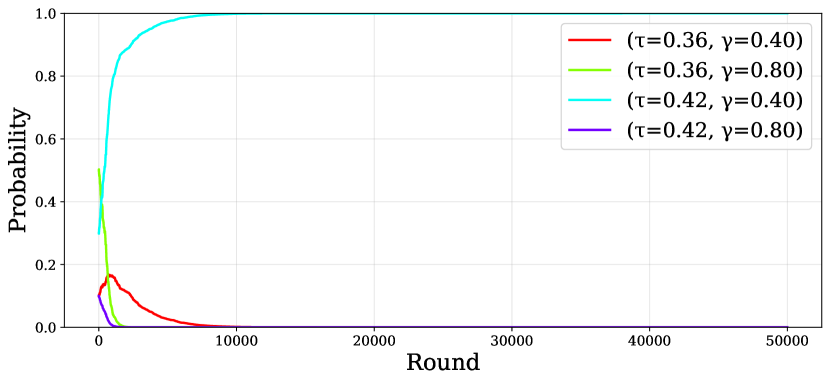
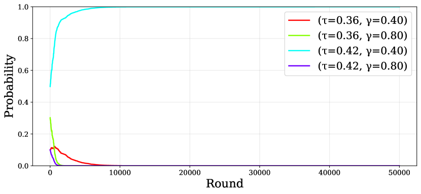
Figure 1: Case - - Exponential weights dynamics for Bank1 (top row) and Bank2 (bottom row), converging to the unique pure NE $((\tau_{h},\gamma_{l}),(\tau_{h},\gamma_{l}))$. Left: known utility matrices. Right: estimated utilities using a single sample per round. $y\sim$ truncated Gaussian ($\mu=0.1,\sigma=0.3$), $\gamma_{l}=0.4$, $\gamma_{h}=0.8$. Initial weights: Bank1 $(0.1,0.5,0.3,0.1)$, Bank2 $(0.1,0.3,0.5,0.1)$

We start with the ‘+ +’ case in Figure 2 (corresponding to Theorem 4 Part II), and see convergence to the unique pure symmetric NE $((\tau_{l},\gamma_{h}),(\tau_{l},\gamma_{h}))$

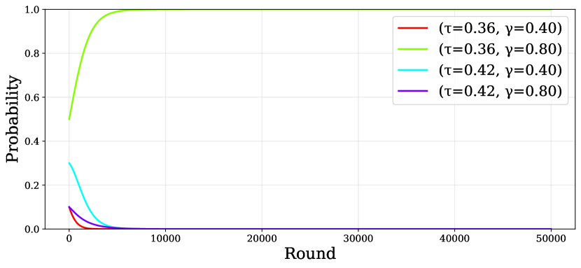
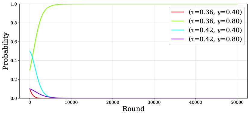
Figure 2: Case + + Exponential weights dynamics for Bank1 (top row) and Bank2 (bottom row), converging to the unique pure NE $((\tau_{l},\gamma_{h}),(\tau_{l},\gamma_{h}))$. Left: known utility matrices. Right: estimated utilities using a single sample per round. $y\sim$ truncated Gaussian ($\mu=0.3,\sigma=0.1$), $\gamma_{l}=0.4$, $\gamma_{h}=0.8$. Initial weights: Bank1 $(0.1,0.5,0.3,0.1)$, Bank2 $(0.1,0.3,0.5,0.1)$.

We now present two representative figures for the ‘$-\,+$’ case. Figure 3 illustrates convergence to the pure asymmetric NE $((\tau_{l},\gamma_{h}),(\tau_{h},\gamma_{l}))$ (corresponding to Theorem 4 Part III), while Figure 4 shows convergence to the mixed symmetric NE $((0,c^{\prime},1-c^{\prime},0),(0,c^{\prime},1-c^{\prime},0))$ (not covered by Theorem 4).

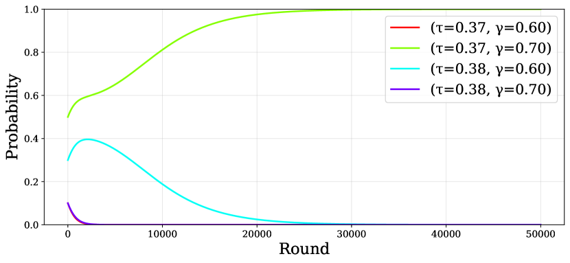
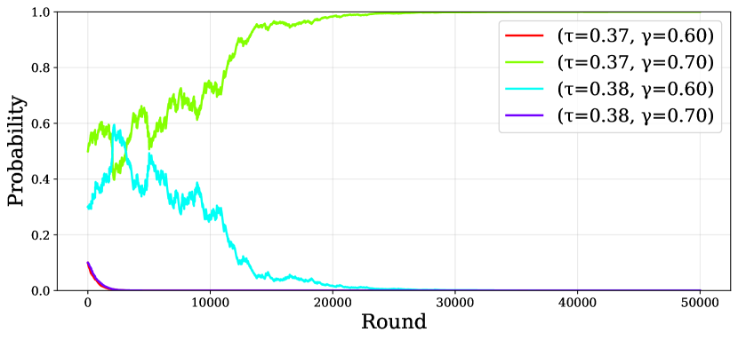
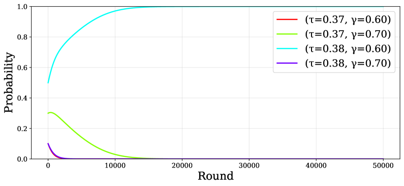
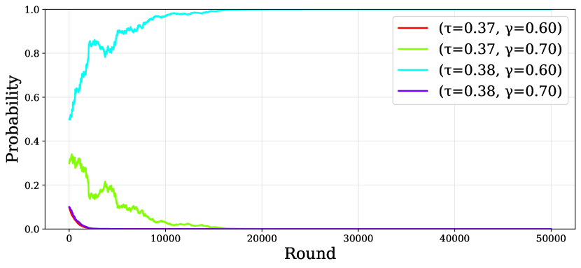
Figure 3: Case - + (a) Exponential weights dynamics for Bank1 (top row) and Bank2 (bottom row) converging to the pure NE $((\tau_{l},\gamma_{h}),(\tau_{h},\gamma_{l}))$, one of the three NE from theory. Left: known utility matrices. Right: estimated utilities using a single sample per round. Parameters: $\epsilon_{1}<0,\epsilon_{2}>0$, $y\sim$ piecewise uniform distribution, $\gamma_{l}=0.6$, $\gamma_{h}=0.7$. Initial weights: Bank1 $(0.1,0.5,0.3,0.1)$, Bank2 $(0.1,0.3,0.5,0.1)$.

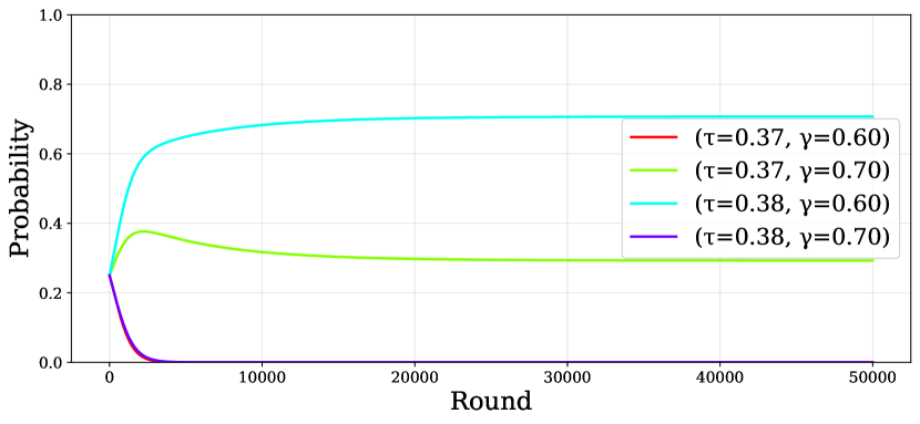
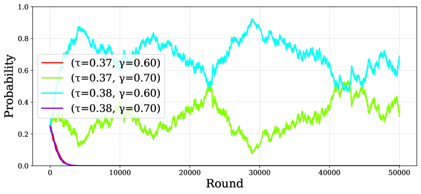
Figure 4: Case - + (b) Exponential weights dynamics for Bank1 (top row) and Bank2 (bottom row) converging to the mixed NE $((0,c,1-c,0),(0,c,1-c,0))$, one of the three NE from theory. Left: known utility matrices. Right: estimated utilities using a single sample per round. Parameters: $\epsilon_{1}<0,\epsilon_{2}>0$, $y\sim$ piecewise uniform distribution, $\gamma_{l}=0.6$, $\gamma_{h}=0.7$. Both banks start with weights $(0.25,0.25,0.25,0.25)$.

Finally, we present three figures for the ‘$+\,-$’ case. Figure 5 illustrates convergence to the pure symmetric NE $((\tau_{l},\gamma_{h}),(\tau_{l},\gamma_{h}))$, while Figure 6 shows convergence to the pure symmetric NE $((\tau_{h},\gamma_{l}),(\tau_{h},\gamma_{l}))$. Both of these cases are covered by Theorem 4 Part IV.

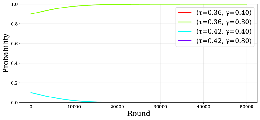
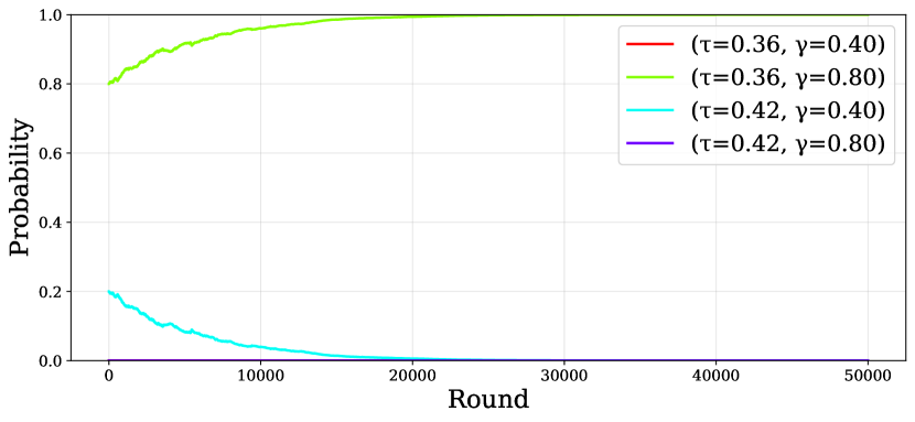
Figure 5: Case + - (a) Exponential weights dynamics for Bank1 (top row) and Bank2 (bottom row), converging to the pure NE $((\tau_{l},\gamma_{h}),(\tau_{l},\gamma_{h})$. Left: known utility matrices. Right: estimated utilities using a single sample per round. $y\sim$ truncated Gaussian ($\mu=0.1,\sigma=0.2$), $\gamma_{l}=0.4$, $\gamma_{h}=0.8$. Initial weights: Bank1 $(0,0.9,0.1,0)$, Bank2 $(0,0.8,0.2,0)$

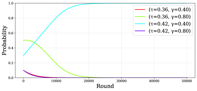
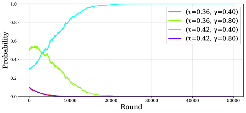
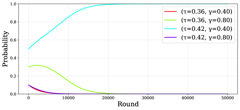
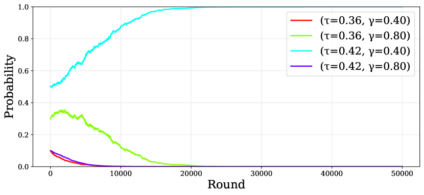
Figure 6: Case + - (b) Exponential weights dynamics for Bank1 (top row) and Bank2 (bottom row), converging to the pure NE $((\tau_{h},\gamma_{l}),(\tau_{h},\gamma_{l}))$. Left: known utility matrices. Right: estimated utilities using a single sample per round. $y\sim$ truncated Gaussian ($\mu=0.1,\sigma=0.2$), $\gamma_{l}=0.4$, $\gamma_{h}=0.8$. Initial weights: Bank1 $(0.1,0.5,0.3,0.1)$, Bank2 $(0.1,0.3,0.5,0.1)$

5.3 Distance to Nash Equilibrium

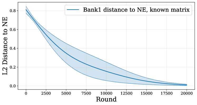
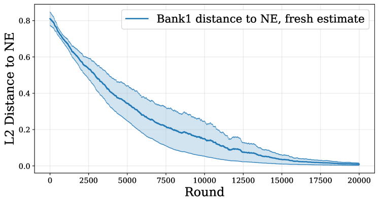
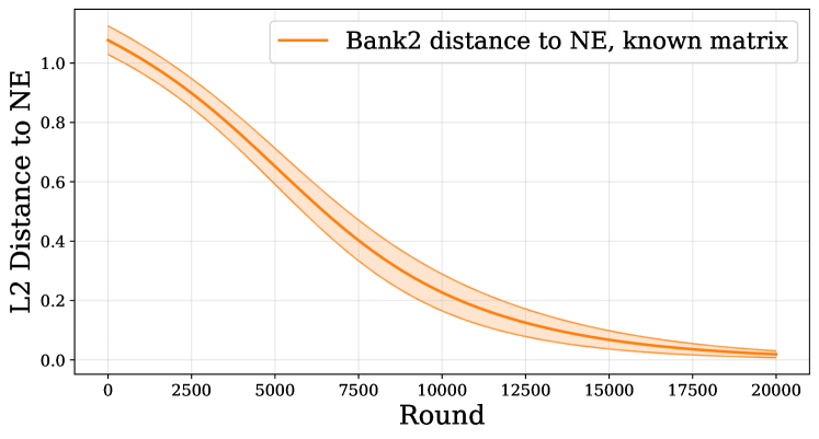
Figure 7: Case + -: Distance of the iterates of Bank 1 (top row) and Bank 2 (bottom row) to the Nash equilibrium. Left: known utility matrices. Right: estimated utilities using a single sample per round. $y\sim$ truncated Gaussian ($\mu=0.1,\sigma=0.2$), $\gamma_{l}=0.4$, $\gamma_{h}=0.8$. Mean(solid) and standard error (shaded) across 5 random initializations.

For the last iterate of Algorithm 1 for both banks, i.e., $p_{1}^{(T)}$ and $p_{2}^{(T)}$, we identify the closest Nash equilibrium $(\theta_{1}^{*},\theta_{2}^{*})$ from the set of Nash equilibria. We then compute the $L_{2}$ distance of each iterate along the trajectory to these equilibrium profiles, $\|p_{1}^{t}-\theta_{1}^{*}\|_{2}$ and $\|p_{2}^{t}-\theta_{2}^{*}\|_{2}$, and plot the mean and standard error across five random initializations. The mean is shown as a solid line, with the shaded region representing the standard error of the mean at each time step $t$. In Figure 7, we show the $L_{2}$ distance to the nearest Nash equilibrium for the $\epsilon_{1}>0,\epsilon_{2}<0$ case. Similar figures for other sign combinations of $(\epsilon_{1},\epsilon_{2})$ are provided in Appendix E. We do note that when estimating the utility matrix using a single sample per round (Algorithm 2 with $n_{sample}=1$), we observe slight deviations in the convergence path due to in-sample errors. However, even in this setting, the algorithm consistently converges to a Nash equilibrium, following a trajectory similar to that in the full-information case.

6 Conclusion and The Future Work

In this work, we investigate the multi-agent performative prediction problem in settings where self-selection effects play a significant role and insensitivity assumptions do not hold. We introduce the ”Bank Game”, in which two mortgage companies compete to set minimum credit score requirements and interest rates. For this simple two-player game, we fully characterize the equilibria and demonstrate that when each player employs Exponential Weights, the dynamics always converge to equilibrium in the last-iterate sense. Finally, we present experimental results that validate our theoretical findings and extend our analysis to scenarios not covered under our assumptions.

Our work also motivates various future directions to explore. A very natural open question is how our results extend to other scenarios in performative prediction where the insensitivity assumption does not hold. More specifically: i) Can we identify additional compelling applications where the insensitivity assumption is violated, finding new use cases for our framework? ii) Can we establish general-purpose results under relaxed insensitivity assumptions? For instance, one promising approach is to analyze cases where this assumption breaks down at specific points in the decision space (e.g., when both banks offer the same rate in our framework, leading to symmetry between players) but holds across most of the decision space. This could yield deeper theoretical insights and broaden the applicability of performative prediction models in multi-agent systems.

Appendix A The Standard Multi-Player Performative Prediction Form

In this section, we rewrite our problem in the multi-player performative prediction form given in [10]. Let:

• $p(y)$: the probability density function of the credit score $y$ under $D_{y}$.

• $g_{1}(\theta_{1},\theta_{2},y)=(1+\gamma_{1})y-(1-y)$: the expected reward of Bank 1 for a customer with score $y$ (if the customer chooses Bank 1).

• $D_{1,\theta_{1},\theta_{2}}$: the distribution of credit score $y$ for customers choosing Bank 1, given strategies $\theta_{1}$ and $\theta_{2}$.

The p.d.f. of $D_{1,\theta_{1},\theta_{2}}$, denoted $p_{1}(\theta_{1},\theta_{2},y)$, is:

$$p_{1}(\theta_{1},\theta_{2},y)=\begin{cases}0,&y<\tau_{1}\text{ or }(\tau_{1},\tau_{2}\leq y\text{ and }\gamma_{1}>\gamma_{2});\\ \frac{p(y)}{Z_{1}(\theta_{1},\theta_{2})},&\tau_{1}\leq y<\tau_{2}\text{ or }(\tau_{1},\tau_{2}\leq y\text{ and }\gamma_{1}<\gamma_{2});\\ \frac{p(y)}{2Z_{1}(\theta_{1},\theta_{2})},&\tau_{1},\tau_{2}\leq y\text{ and }\gamma_{1}=\gamma_{2},\\ \end{cases}$$

where $Z_{1}(\theta_{1},\theta_{2})$ is the normalization constant:

$$Z_{1}(\theta_{1},\theta_{2})=\begin{cases}\int_{\tau_{1}}^{1}p(y)\,dy,&\text{if }\gamma_{1}<\gamma_{2};\\ \frac{1}{2}\int_{\tau_{1}}^{1}p(y)\,dy,&\text{if }\gamma_{1}=\gamma_{2};\\ \int_{\tau_{1}}^{\tau_{2}}p(y)\,dy,&\text{if }\gamma_{1}>\gamma_{2}.\end{cases}$$

Using this, the utility function for Bank 1 can be rewritten as:

$$u_{1}(\theta_{1},\theta_{2})=\mathbb{E}_{y\sim D_{1,\theta_{1},\theta_{2}}}\big{[}g_{1}(\theta_{1},\theta_{2},y)Z_{1}(\theta_{1},\theta_{2})\big{]}.$$

In this performative prediction framework, the distribution $D_{1,\theta_{1},\theta_{2}}$ depends discontinuously on the strategies $\theta_{1}$ and $\theta_{2}$, making it non-Lipschitz. This characteristic highlights the distinctiveness of the model compared to standard performative prediction problems.

Appendix B Property of the $f$ function

We first introduce the following simple lemma about the properties of $f$, which is easy to check based on the definition given in (2).

Lemma 2.

Assume $\emph{Supp}(D_{y})=[0,1]$. We have the following:

1. Let $\tau_{a}<\tau_{b}<\tau_{c}$. Then $f_{D_{y}}(\gamma_{1},\tau_{a},\tau_{c})=f_{D_{y}}(\gamma_{1},\tau_{a},\tau_{b})+f_{D_{y}}(\gamma_{1},\tau_{b},\tau_{c})$.

2. $f(\gamma,\tau_{a},\tau_{b})$ is monotonically increasing with respect to $\gamma$.

3. We have $f(\gamma,\tau_{a},\tau_{b})\in[-1,2]$.

4. Let $y_{\gamma}=\frac{1}{2+\gamma}$. If $y_{\gamma}\in(\tau_{a},\tau_{b})$, then $f(\gamma,\tau_{a},y_{\gamma})<0$, and $f(\gamma,y_{\gamma},\tau_{b})>0$.

Proof.

We first recall the definition of $f$:

$$f_{D_{y}}(\gamma,\tau_{a},\tau_{b})=\int_{\tau_{a}}^{\tau_{b}}[(2+\gamma)y-1]p(y)dy.$$

The first property can be easily obtained based on the integration form. For the second property, it can be seen that for any $\delta>0$,

$$f(\gamma+\delta,\tau_{a},\tau_{b})=f(\gamma,\tau_{a},\tau_{b})+\int_{\tau_{a}}^{\tau_{b}}\delta yp(y)dy>f(\gamma,\tau_{a},\tau_{b}).$$

For the third property, we have

$$-1=\min_{y\in[0,1]}(2+\gamma)y-1\leq f(\gamma,\tau_{a},\tau_{b})\leq\max_{y\in[0,1]}(2+\gamma)y-1\leq 2.$$

For the last property, it can be proved by noticing that $(2+\gamma)y_{\gamma}-1=0$. ∎

Appendix C Proofs for Section 3: Equilibrium Characterization

In this section, we provide the proof of the conclusions given in Section 3.

C.1 Proof of Theorem 1

Since the utility matrix of this problem can be represented as a $4\times 4$ matrix, the pure Nash equilibria (NE) can be obtained by analyzing the asymmetric best response dynamics. Consider a dynamic process where Banks 1 and 2 alternately update their strategies by playing their best responses, conditioned on observing the opponent’s decisions. Based on different initializations (all four decisions) for Bank 2, we obtain the results shown in Figure 12 under various conditions. The figure clearly illustrates the pure Nash equilibria for different scenarios.

Figure 8: $\epsilon_{1}<0,\epsilon_{2}>0$.

Figure 9: $\epsilon_{1}>0,\epsilon_{2}>0$.

Figure 10: $\epsilon_{1}<0,\epsilon_{2}<0$.

Figure 11: $\epsilon_{1}>0,\epsilon_{2}<0$.

Figure 12: Alternative Best Response Dynamics. * The arrows means that, if bank 2 picks decision $(\tau_{\ell},\gamma_{\ell})$, the best response for Bank 1 is $(\tau_{h},\gamma_{\ell})$. ** The dashed arrow means that both case can happen, which depends on specific conditions on $D_{y}$. Note that it does not have an influence on the final conclusion, since both cases converge to the NE in the end.

C.2 Proof of Theorem 2

We overload notation and denote the expected utility of bank $i$ under $p_{1}$ and $p_{2}$ as:

$$u_{i}(p_{1},p_{2})=\mathbb{E}_{\theta_{1}\sim p_{1},\theta_{2}\sim p_{2}}[u_{i}(\theta_{1},\theta_{2})].$$

Firstly, note that, based on Table 1 and Lemma 2, it can be easily shown that for any $\theta\in\{\theta^{(j)}\}_{j=1}^{4}$,

$$u_{1}(\theta^{(3)},\theta)>u_{1}(\theta^{(1)},\theta).$$

More specifically,

$$\begin{split}u_{1}(\theta^{(3)},\theta^{(1)})={}&\frac{1}{2}f(\gamma_{\ell},\tau_{h},1)>\frac{1}{2}f(\gamma_{\ell},\tau_{\ell},1)=u_{1}(\theta^{(1)},\theta^{(1)}),\\ u_{1}(\theta^{(3)},\theta^{(2)})={}&f(\gamma_{\ell},\tau_{h},1)>f(\gamma_{\ell},\tau_{\ell},1)=u_{1}(\theta^{(1)},\theta^{(2)}),\\ u_{1}(\theta^{(3)},\theta^{(3)})={}&\frac{1}{2}f(\gamma_{\ell},\tau_{h},1)>f(\gamma_{\ell},\tau_{\ell},\tau_{h})+\frac{1}{2}f(\gamma_{\ell},\tau_{h},1)=u_{1}(\theta^{(1)},\theta^{(3)}),\\ u_{1}(\theta^{(3)},\theta^{(4)})={}&f(\gamma_{\ell},\tau_{h},1)>f(\gamma_{\ell},\tau_{\ell},1)=u_{1}(\theta^{(1)},\theta^{(4)}),\end{split}$$

where the first, second and last inequality is because based on Lemma 2,

$$f(\gamma_{\ell},\tau_{\ell},1)=\underbrace{f(\gamma_{\ell},\tau_{\ell},\tau_{h})}_{<0}+f(\gamma_{\ell},\tau_{h},\tau_{h}),$$

and the third inequality is because $f(\gamma_{\ell},\tau_{\ell},\tau_{h})<0.$ This implies that $\theta^{(1)}$ is strictly dominated by $\theta^{(3)}$, and will not be part of the mixed NE.

Since the game is symmetric, the same argument holds true for Bank 2, i.e. $u_{2}(\theta,\theta^{(3)})>u_{2}(\theta,\theta^{(1)})$. By a similar argument, for any $\theta\in\{\theta^{(j)}\}_{j=2}^{4}$, we have

$$u_{1}(\theta^{(2)},\theta)>u_{1}(\theta^{(4)},\theta),$$

which indicates that $\theta^{(4)}$ will also not be part of mixed NE for Bank 1 or Bank 2. To summarize, any mixed NE must satisfy $p_{1,1}=p_{1,4}=p_{2,1}=p_{2,4}=0$.

Consider a pair of mixed strategies $p_{1}=[0,p_{1,2},1-p_{1,2},0]$ and $p_{2}=[0,p_{2,2},1-p_{2,2},0]$. Then the utility of Bank 1 can be written as:

$$\begin{split}u_{1}(p_{1},p_{2})={}&\frac{1}{2}p_{1,2}p_{2,2}f(\gamma_{h},\tau_{\ell},1)+p_{1,2}(1-p_{2,2})f(\gamma_{h},\tau_{\ell},\tau_{h})+(1-p_{1,2})p_{2,2}f(\gamma_{\ell},\tau_{h},1)\\ {}&+\frac{(1-p_{1,2})(1-p_{2,2})}{2}f(\gamma_{\ell},\tau_{h},1)\\ ={}&\frac{1}{2}p_{1,2}\left[(2-p_{2,2})f(\gamma_{h},\tau_{\ell},\tau_{h})+p_{2,2}f(\gamma_{h},\tau_{h},1)-(1+p_{2,2})f(\gamma_{\ell},\tau_{h},1)\right]\\ {}&+\frac{(p_{2,2}+1)}{2}f(\gamma_{\ell},\tau_{h},1).\end{split}$$ (6)

Note that it is a linear function with respect to $p_{1,2}$, and the slope is given by:

$$\begin{split}{}&\frac{1}{2}\left[(2-p_{2,2})f(\gamma_{h},\tau_{\ell},\tau_{h})+p_{2,2}f(\gamma_{h},\tau_{h},1)-(1+p_{2,2})f(\gamma_{\ell},\tau_{h},1)\right]\\ ={}&\frac{1}{2}p_{2,2}[f(\gamma_{h},\tau_{h},1)-f(\gamma_{\ell},\tau_{h},1)-f(\gamma_{h},\tau_{\ell},\tau_{h})]+f(\gamma_{h},\tau_{\ell},\tau_{h})-\frac{1}{2}f(\gamma_{\ell},\tau_{h},1),\end{split}$$

Let

$$g(p)=p[f(\gamma_{h},\tau_{h},1)-f(\gamma_{\ell},\tau_{h},1)-f(\gamma_{h},\tau_{\ell},\tau_{h})]+2f(\gamma_{h},\tau_{\ell},\tau_{h})-f(\gamma_{\ell},\tau_{h},1).$$ (7)

Then, the slope of $u(p_{1},p_{2})$ with respect to $p_{1,2}$ is given by $\frac{1}{2}g(p_{2,2})$. Moreover, (recalling our definitions of the shorthand notation $\epsilon_{1}=\frac{1}{2}f(\gamma_{h},\tau_{\ell},1)-f(\gamma_{\ell},\tau_{h},1)$ and $\epsilon_{2}=f(\gamma_{h},\tau_{\ell},\tau_{h})-\frac{1}{2}f(\gamma_{\ell},\tau_{h},1)$), we note that $g(p):[0,1]\mapsto\mathbb{R}$ is a linear function, $g(0)=2\epsilon_{2}$, and $g(1)=2\epsilon_{1}$.

Let $BR_{1}(p)\subseteq[0,1]$ denote the candidate set of best response probabilities of picking $\theta^{(2)}$ of Bank 1 if Bank 2 picks $p_{2}=[0,p,1-p,0]$. The corresponding candidate set for Bank 2 is denoted by $BR_{2}(p)$.

Then, consider the following cases:

Case 1:

$\epsilon_{1}<0$, $\epsilon_{2}<0$. Therefore, $g(0)=2\epsilon_{2}<0$ and $g(1)=2\epsilon_{1}<0$, then it is clear that $g(p)<0$ for all $p\in[0,1]$. This means that the slope in (6) will always be negative, so $BR_{1}(p)=\{0\}$ for any $p\in[0,1]$. Similarly, $BR_{2}(p)=\{0\}$ for any $p\in[0,1]$, which indicates that $p_{1,2}=p_{2,2}=0$, $p_{1,3}=p_{2,3}=1$ is the only mixed NE (and, in fact, this corresponds to a pure NE).

Case 2:

$\epsilon_{1}<0$, $\epsilon_{2}>0$. Therefore, $g(0)>0$, and $g(1)<0$, and since $g$ is a linear function, it means that there must exist a unique $c\in(0,1)$, such that $g(c)=0$. Based on (7), we know

$$c=\frac{f(\gamma_{\ell},\tau_{h},1)-2f(\gamma_{h},\tau_{\ell},\tau_{h})}{f(\gamma_{h},\tau_{h},1)-f(\gamma_{\ell},\tau_{h},1)-f(\gamma_{h},\tau_{\ell},\tau_{h})}.$$

Combining with (6), we have

$$BR_{1}(p)=\begin{cases}\{0\},&p>c;\\ \{1\},&p<c;\\ [0,1],&p=c.\end{cases}$$

This is because, if $p>c$, $g(p)<0$, so the slope in (6) is negative, and $BR_{1}(p)=\{0\}$.If $p<c$, then $g(p)>0$, the slope in (6) is positive, and $BR_{1}(p)=\{1\}$. If $p=c$, (6) will not be a function of $p_{1,2}$, so any decision for Bank 1 leads to the same gain. Similarly, we have

$$BR_{2}(p)=\begin{cases}\{0\},&p>c;\\ \{1\},&p<c;\\ [0,1],&p=c.\end{cases}$$

Therefore, we know that $([0,c,1-c,0],[0,c,1-c,0])$ is a mixed NE, and $([0,0,1,0],[0,1,0,0])$ and $([0,1,0,0],[0,0,1,0])$ are also pure NEs.

Case 3:

$\epsilon_{1}>0$, $\epsilon_{2}<0$. Therefore, $g(0)<0$, and $g(1)>0$, and since $g$ is a linear function, it means that there must exist $c\in(0,1)$, such that $g(c)=0$. Combining with (6), we have

$$BR_{1}(p)=\begin{cases}\{1\},&p>c;\\ \{0\},&p<c;\\ [0,1],&p=c.\end{cases}$$

Similarly, we have

$$BR_{2}(p)=\begin{cases}\{1\},&p>c;\\ \{0\},&p<c;\\ [0,1],&p=c.\end{cases}$$

Therefore, we know that $([0,c,1-c,0],[0,c,1-c,0])$ is a mixed NE, and $([0,0,1,0],[0,0,1,0])$ and $([0,1,0,0],[0,1,0,0])$ are also pure NEs.

Case 4:

$\epsilon_{1}>0$, $\epsilon_{2}>0$. In this case, we know that $g(p)>0$ for all $p\in[0,1]$. Then, we have $BR_{1}(p)=\{1\}$, and $BR_{2}(p)=\{1\}$, which implies that the only mixed NE here is $([0,1,0,0],[0,1,0,0])$ (which is in fact a pure NE). This completes the proof of the theorem.

C.3 Proof of Theorem 3

Firstly, we know $u_{i}(\theta^{(3)},\theta)>u_{i}(\theta^{(1)},\theta),$. This means $\theta^{(1)}$ will not be part of CE. Conditioned on this, for any $\theta\in\{\theta^{(j)}\}_{j=2}^{4}$, we have $u_{1}(\theta^{(2)},\theta)>u_{1}(\theta^{(4)},\theta).$ This indicates that $\theta^{(4)}$ will no be part of CE. Thus, $p_{11}=\dots,=p_{14}=0$, $p_{11}=\dots,=p_{41}=0$, $p_{14}=\dots,=p_{44}=0$, $p_{41}=\dots,=p_{44}=0$. Next, based on Definition 2, we firstly need:

$$\begin{split}\sum_{i=2}^{3}u_{1}\left((\tau_{\ell},\gamma_{h}),\theta^{(i)}\right)p_{2i}\geq{}&\sum_{i=2}^{3}u_{1}\left(\theta^{\prime},\theta^{(i)}\right)p_{2i},\ \forall\theta^{\prime}\in\Theta,\end{split}$$

That is, for $\theta^{\prime}=\theta^{(1)}$,

$$\begin{split}p_{22}\frac{1}{2}f(\gamma_{h},\tau_{\ell},1)+p_{23}f(\gamma_{h},\tau_{\ell},\tau_{h})\geq p_{22}f(\gamma_{\ell},\tau_{\ell},1)+p_{23}(f(\gamma_{\ell},\tau_{\ell},\tau_{h})+\frac{1}{2}f(\gamma_{\ell},\tau_{h},1)),\end{split}$$

that is,

$$p_{22}(\epsilon_{1}-f(\gamma_{\ell},\tau_{\ell},\tau_{h}))\geq p_{23}(f(\gamma_{\ell},\tau_{\ell},\tau_{h})-\epsilon_{2}),$$

that is

$$p_{22}\epsilon_{1}\geq-p_{23}\epsilon_{2}+(p_{22}+p_{23})f(\gamma_{\ell},\tau_{\ell},\tau_{h}).$$ (8)

For $\theta^{\prime}=\theta^{(3)}$, we have

$$p_{22}\epsilon_{1}\geq-p_{23}\epsilon_{2}.$$ (9)

Note that since $f(\gamma_{\ell},\tau_{\ell},\tau_{h})$ is negative, we know that (9) implies (8), and thus (8) can be dropped.

For $\theta^{\prime}=\theta^{(4)}$, we have

$$\begin{split}p_{22}\frac{1}{2}f(\gamma_{h},\tau_{\ell},1)+p_{23}f(\gamma_{h},\tau_{\ell},\tau_{h})\geq p_{22}\frac{1}{2}f(\gamma_{h},\tau_{h},1)+p_{23}0,\end{split}$$

which always holds true. Next, we need

$$\begin{split}\sum_{i=2}^{3}u_{1}\left((\tau_{h},\gamma_{\ell}),\theta^{(i)}\right)p_{3i}\geq{}&\sum_{i=2}^{3}u_{1}\left(\theta^{\prime},\theta^{(i)}\right)p_{3i},\ \forall\theta^{\prime}\in\Theta.\end{split}$$

For $\theta^{\prime}=\theta^{(1)}$, it means

$$p_{32}f(\gamma_{\ell},\tau_{h},1)+p_{33}\frac{1}{2}f(\gamma_{\ell},\tau_{h},1)\geq p_{32}f(\gamma_{\ell},\tau_{\ell},1)+p_{33}\left(f(\gamma_{\ell},\tau_{\ell},\tau_{h})+\frac{1}{2}f(\gamma_{\ell},\tau_{h},1)\right),$$

which always holds true. For $\theta^{\prime}=\theta^{(2)}$, we have

$$-p_{32}\epsilon_{1}\geq p_{33}\epsilon_{2}.$$

For $\theta^{\prime}=\theta^{(4)}$, we have

$$p_{32}f(\gamma_{\ell},\tau_{h},1)+p_{33}\frac{1}{2}f(\gamma_{\ell},\tau_{h},1)\geq p_{32}\frac{1}{2}f(\gamma_{h},\tau_{h},1).$$

Rearrange, we have

$$-p_{32}\epsilon_{1}\geq p_{33}\epsilon_{2}-\left(p_{33}+\frac{1}{2}p_{32}\right)f(\gamma_{h},\tau_{\ell},\tau_{h}).$$

Since $f(\gamma_{h},\tau_{\ell},\tau_{h})$ is positive, the above condition is implied by $-p_{32}\epsilon_{1}\geq p_{33}\epsilon_{2},$ and thus can be dropped.

To proceed, we need

$$\begin{split}\sum_{i=2}^{3}u_{2}\left(\theta^{(i)},(\tau_{\ell},\gamma_{h})\right)p_{i2}\geq{}&\sum_{i=2}^{3}u_{2}\left(\theta^{(i)},\theta^{\prime}\right)p_{i2},\ \forall\theta^{\prime}\in\Theta,\end{split}$$

which is equivalent to

$$\begin{split}\sum_{i=2}^{3}u_{1}\left((\tau_{\ell},\gamma_{h}),\theta^{(i)}\right)p_{i2}\geq{}&\sum_{i=2}^{3}u_{1}\left(\theta^{\prime},\theta^{(i)}\right)p_{i2},\ \forall\theta^{\prime}\in\Theta.\end{split}$$

Thus, following similar procedure, the condition we get is

$$p_{22}\epsilon_{1}\geq-p_{32}\epsilon_{2}.$$

Finally, for

$$\begin{split}\sum_{i=2}^{3}u_{2}\left(\theta^{(i)},(\tau_{h},\gamma_{\ell})\right)p_{i3}\geq{}&\sum_{i=2}^{3}u_{2}\left(\theta^{(i)},\theta^{\prime}\right)p_{i3},\ \forall\theta^{\prime}\in\Theta,\end{split}$$

we get

$$-p_{23}\epsilon_{1}\geq p_{33}\epsilon_{2},$$

To summarize, we have the following conditions:

$$p_{22}\epsilon_{1}\geq{} -p_{23}\epsilon_{2}$$ (10)

$$-p_{32}\epsilon_{1}\geq{} p_{33}\epsilon_{2}.$$ (11)

$$p_{22}\epsilon_{1}\geq{} -p_{32}\epsilon_{2}$$ (12)

$$-p_{23}\epsilon_{1}\geq{} p_{33}\epsilon_{2},$$ (13)

When $\epsilon_{1}>0$ and $\epsilon_{2}>0$, from (11) and (13), we know that $p_{32}=p_{33}=p_{23}=0$, which leads to $p_{22}=1$, and it can make sure all inequality is ture. Similarly, when $\epsilon_{1}<0$ and $\epsilon_{2}<0$, we get $p_{22}=p_{32}=p_{23}=0$, and $p_{33}=1$.

When $\epsilon_{1}>0,\epsilon_{2}<0$, we need $\min\{p_{22},p_{33}\}>\max\left\{\frac{|\epsilon_{2}|}{\epsilon_{1}}p_{23},\frac{\epsilon_{1}}{|\epsilon_{2}|}p_{32}\right\}$. For $\epsilon_{1}<0$ and $\epsilon_{2}>0$, we need $\min\{p_{23},p_{32}\}>\max\left\{\frac{|\epsilon_{1}|}{\epsilon_{2}}p_{22},\frac{\epsilon_{2}}{|\epsilon_{1}|}p_{33}\right\}$.

Appendix D Proofs for Section 4: Convergence of Dynamics

D.1 Proof of Lemma 1

We have for $t>1$,

$$\begin{split}\frac{p^{(t+1)}_{1,1}}{p^{(t+1)}_{1,3}}={}&\frac{p^{(t)}_{1,1}\exp\left(\eta\sum_{j=1}^{4}p_{2,j}^{(t)}u_{1}\left(\theta^{(1)},\theta^{(j)}\right)\right)}{p^{(t)}_{1,3}\exp\left(\eta\sum_{j=1}^{4}p_{2,j}^{(t)}u_{1}\left(\theta^{(3)},\theta^{(j)}\right)\right)}=\frac{p_{1,1}^{(t)}}{p_{1,3}^{(t)}}\exp\left(\eta\sum_{j=1}^{4}p_{2,j}^{(t)}\left(u_{1}\left(\theta^{(1)},\theta^{(j)}\right)-u_{1}\left(\theta^{(3)},\theta^{(j)}\right)\right)\right)\\ \leq{}&\frac{p_{1,1}^{(t)}}{p_{1,3}^{(t)}}\exp\left(-\eta\xi_{1}\right),\end{split}$$

where recall that we defined $\xi_{1}:=\min\{\frac{1}{2}\left|f(\gamma_{\ell},\tau_{\ell},\tau_{h})\right|,\frac{1}{2}|f(\gamma_{h},\tau_{\ell},\tau_{h})|,|\epsilon_{1}|,|\epsilon_{2}|\}>0$ as shorthand. Therefore, we have

$${p^{(t+1)}_{1,1}}\leq p_{1,3}^{(t+1)}\frac{p^{(1)}_{1,1}}{p^{(1)}_{1,3}}\left[\exp\left(-\eta\xi_{1}\right)\right]^{t}\leq\frac{p^{(1)}_{1,1}}{p^{(1)}_{1,3}}\left[\exp\left(-\eta\xi_{1}\right)\right]^{t}\leq c_{ini}\left[\exp\left(-\eta\xi_{1}\right)\right]^{t},$$

where the last inequality plugs in the definition of $c_{ini}=\max_{i\in[2]}\left\{\frac{\max_{j\in[4]}p^{(1)}_{i,j}}{\min_{i\in[4]}p^{(1)}_{i,j}}\right\}$. Similarly, we also have

$$\begin{split}\frac{p^{(t+1)}_{2,1}}{p^{(t+1)}_{2,3}}={}&\frac{p^{(t)}_{2,1}\exp\left(\eta\sum_{j=1}^{4}p_{1,j}^{(t)}u_{2}\left(\theta^{(j)},\theta^{(1)}\right)\right)}{p^{(t)}_{2,3}\exp\left(\eta\sum_{j=1}^{4}p_{1,j}^{(t)}u_{2}\left(\theta^{(j)},\theta^{(3)}\right)\right)}=\frac{p_{2,1}^{(t)}}{p_{2,3}^{(t)}}\exp\left(\eta\sum_{j=1}^{4}p_{1,j}^{(t)}\left(u_{1}\left(\theta^{(1)},\theta^{(j)}\right)-u_{1}\left(\theta^{(3)},\theta^{(j)}\right)\right)\right)\\ \leq{}&\frac{p_{2,1}^{(t)}}{p_{2,3}^{(t)}}\exp\left(-\eta\xi_{1}\right),\end{split}$$

where the second equality is based on the fact the game is symmetric. It implies that

$${p^{(t+1)}_{2,1}}\leq c_{ini}\left[\exp\left(-\eta\xi_{1}\right)\right]^{t}.$$

Next, we know that $u_{1}(\theta^{(2)},\theta^{(1)})=u_{1}(\theta^{(4)},\theta^{(1)})=0$, but for all $j\neq 1$, we have $u_{1}\left(\theta^{(2)},\theta^{(j)}\right)-u_{1}\left(\theta^{(4)},\theta^{(j)}\right)\geq\xi_{1}$. Therefore, we have for all $t>1$,

$$\begin{split}\frac{p^{(t+1)}_{1,4}}{p^{(t+1)}_{1,2}}=\frac{p^{(t)}_{1,4}}{p^{(t)}_{1,2}}\exp\left(\eta\sum_{j=2}^{4}p^{(t)}_{2,j}\left(u_{1}\left(\theta^{(4)},\theta^{(j)}\right)-u_{1}\left(\theta^{(2)},\theta^{(j)}\right)\right)\right)\leq\frac{p^{(t)}_{1,4}}{p^{(t)}_{1,2}}\exp\left(-\eta\xi_{1}\sum_{j=2}^{4}p^{(t)}_{2,j}\right).\end{split}$$ (14)

Note that it implies that the ratio between $p_{1,4}^{(t)}$ and $p_{1,2}^{(t)}$ is non-increasing. Moreover, we have just shown that

$$p_{2,1}^{(t)}\leq c_{ini}\exp\left(-\eta\xi_{1}(t-1)\right)$$

For $t\geq t^{\prime}=\max\left\{\left\lceil\frac{\log 2c_{ini}}{\epsilon\eta}+1\right\rceil,2\right\}$, we have $p_{2,1}^{(t)}\leq\frac{1}{2}$, which implies that

$$\sum_{j=2}^{4}p_{2,j}^{(t)}=1-p_{1,2}^{(t)}\geq\frac{1}{2}.$$

Thus,

$$\begin{split}\frac{p^{(t+1)}_{1,4}}{p^{(t+1)}_{1,2}}\leq{}&\frac{p^{(t)}_{1,4}}{p^{(t)}_{1,2}}\exp\left(-\eta\xi_{1}\sum_{j=2}^{4}p^{(t)}_{2,j}\right)\leq\frac{p^{(t^{\prime}-1)}_{1,4}}{p^{(t^{\prime}-1)}_{1,2}}\left(\exp\left(-\frac{1}{2}\eta\xi_{1}\right)\right)^{t-t^{\prime}+1}\exp\left(-\eta\xi_{1}\sum_{j=2}^{4}p_{2,j}^{(t^{\prime}-1)}\right)\\ \leq{}&\frac{p^{(1)}_{1,4}}{p^{(1)}_{1,2}}\left(\exp\left(-\frac{1}{2}\eta\xi_{1}\right)\right)^{t-t^{\prime}+1}\leq c_{ini}\exp\left(-\frac{1}{2}\eta\xi_{1}(t-t^{\prime}+1)\right).\end{split}$$

where the penultimate inequality uses Equation (14) recursively for $t=t^{\prime}-1,\ldots,1$. We complete the proof by setting

$$c_{ini}\exp\left(-\frac{1}{2}\eta\xi_{1}(t-t^{\prime}+1)\right)\leq\omega.$$

D.2 Proof of Theorem 4

In this section, we present the proof of Theorem 4, considering four cases based on the different possible signs of $\epsilon_{1}$ and $\epsilon_{2}$.
Recall the definitions $\epsilon_{1}=\frac{1}{2}f(\gamma_{h},\tau_{\ell},1)-f(\gamma_{\ell},\tau_{h},1)$ and $\epsilon_{2}=f(\gamma_{h},\tau_{\ell},\tau_{h})-\frac{1}{2}f(\gamma_{\ell},\tau_{h},1)$. Also recall the shorthand definitions $\xi_{1}=\min\{\frac{1}{2}f(\gamma_{\ell},\tau_{h},1),\frac{1}{2}\left|f(\gamma_{\ell},\tau_{\ell},\tau_{h})\right|,\frac{1}{2}|f(\gamma_{h},\tau_{\ell},\tau_{h})|,|\epsilon_{1}|,|\epsilon_{2}|\}>0$ and $c_{ini}:=\max_{i\in[2]}\left\{\frac{\max_{j\in[4]}p^{(1)}_{i,j}}{\min_{i\in[4]}p^{(1)}_{i,j}}\right\}$.

Case I: $\epsilon_{1}<0,$ and $\epsilon_{2}<0$. We have

$$\begin{split}\frac{p^{(t+1)}_{1,2}}{p^{(t+1)}_{1,3}}={}&\frac{p^{(t)}_{1,2}}{p^{(t)}_{1,3}}\exp\left(\eta\sum_{j=1}^{4}p^{(t)}_{2,j}\left(u_{1}\left(\theta^{(2)},\theta^{(j)}\right)-u_{1}\left(\theta^{(3)},\theta^{(j)}\right)\right)\right)\\ \leq{}&\frac{p^{(t)}_{1,2}}{p^{(t)}_{1,3}}\exp\left(-\eta\sum_{j=1}^{3}p^{(t)}_{2,j}\xi_{1}+p^{(t)}_{2,4}\left(f(\gamma_{h},\tau_{\ell},\tau_{h})+\frac{1}{2}f(\gamma_{h},\tau_{h},1)-f(\gamma_{\ell},\tau_{h},1)\right)\right)\\ \leq{}&\frac{p^{(t)}_{1,2}}{p^{(t)}_{1,3}}\exp\left(-\eta\sum_{j=1}^{3}p^{(t)}_{2,j}\xi_{1}+3\eta p^{(t)}_{2,4}\right)=\frac{p^{(t)}_{1,2}}{p^{(t)}_{1,3}}\exp\left(-\eta\sum_{j=1}^{4}p^{(t)}_{2,j}\xi_{1}+\eta(\xi_{1}+3)p^{(t)}_{2,4}\right)\\ ={}&\frac{p^{(t)}_{1,2}}{p^{(t)}_{1,3}}\exp\left(-\eta\xi_{1}+\eta(\xi_{1}+3)p^{(t)}_{2,4}\right).\\ \end{split}$$ (15)

For the first inequality, it is because:

$$\begin{split}u_{1}(\theta^{(2)},\theta^{(1)})-u_{1}(\theta^{(3)},\theta^{(1)})={}&0-\frac{1}{2}f(\gamma_{\ell},\tau_{h},1)\leq-\xi_{1},\\ u_{1}(\theta^{(2)},\theta^{(2)})-u_{1}(\theta^{(3)},\theta^{(2)})={}&\frac{1}{2}f(\gamma_{h},\tau_{\ell},1)-f(\gamma_{\ell},\tau_{h},1)=\epsilon_{1}\leq-\xi_{1},\\ u_{1}(\theta^{(2)},\theta^{(3)})-u_{1}(\theta^{(3)},\theta^{(3)})={}&f(\gamma_{h},\tau_{\ell},\tau_{h})-\frac{1}{2}f(\gamma_{\ell},\tau_{h},1)=\epsilon_{2}\leq-\xi_{1}.\end{split}$$

The second inequality of (15) is because the $f$ function is upper bounded by 2 based on Lemma 2, and $f(\gamma_{\ell},\tau_{h},1)$ is positive. Denote as shorthand the constant $t^{\prime\prime}=t^{\prime}+1+\left\lceil\frac{2}{\eta\xi_{1}}\log\frac{2(\xi_{1}+3)c_{ini}}{\xi_{1}}\right\rceil$. Then, from Lemma 1, we have for $t\geq t^{\prime\prime}$,

$$\eta(\xi_{1}+3)p_{2,4}^{(t)}\leq\frac{\eta\xi_{1}}{2}.$$

Thus, we have

$$\begin{split}\frac{p^{(t+1)}_{1,2}}{p^{(t+1)}_{1,3}}\leq{}&\frac{p^{(t)}_{1,2}}{p^{(t)}_{1,3}}\exp\left(-\frac{\eta\xi_{1}}{2}\right)\ldots\leq\frac{p^{(t^{\prime\prime}-1)}_{1,2}}{p^{(t^{\prime\prime}-1)}_{1,3}}\left[\exp\left(-\frac{\eta\xi_{1}}{2}\right)\right]^{t-t^{\prime\prime}+1}\\ \leq{}&c_{\text{ini}}\exp\left(3\eta t^{\prime\prime}\right)\exp\left(-\frac{\eta\xi_{1}}{2}\left(t-t^{\prime\prime}+1\right)\right),\end{split}$$

where the last inequality is obtained by applying the following inequality recursively for $t=t^{\prime\prime}-1,\dots,1$:

$$\frac{p^{(t)}_{1,2}}{p^{(t)}_{1,3}}\leq\frac{p^{(t-1)}_{1,2}}{p^{(t-1)}_{1,3}}\exp\left(-\eta\xi_{1}+\eta(\xi_{1}+3)p^{(t-1)}_{2,4}\right)\leq\frac{p^{(t-1)}_{1,2}}{p^{(t-1)}_{1,3}}\exp(3\eta),$$

which is obtained based on (15).

Note that $t^{\prime\prime}$ is a constant. We have for $t\geq t^{\prime\prime}$,

$$p^{(t+1)}_{1,2}\leq c_{\text{ini}}\exp\left(3\eta t^{\prime\prime}\right)\exp\left(-\frac{\eta\xi_{1}}{2}\left(t-t^{\prime\prime}+1\right)\right),$$

and thus

$$p^{(t+1)}_{1,3}\geq\max\left\{1-3c_{\text{ini}}\exp\left(3\eta t^{\prime\prime}\right)\exp\left(-\frac{\eta\xi_{1}}{2}\left(t-t^{\prime\prime}+1\right)\right),0\right\}$$

The proof is completed by setting

$$c_{\text{ini}}\exp\left(3\eta t^{\prime\prime}\right)\exp\left(-\frac{\eta\xi_{1}}{2}\left(t-t^{\prime\prime}+1\right)\right)\leq\omega.$$

It shows that $p_{1,2}^{(t)}$ converges to 0 at an exponential rate after $t^{\prime\prime}$ iterations, which is a constant factor. Combining with Lemma 1, we can draw the conclusion that $p_{1,3}^{(t)}$ converges to 1 exponentially fast after a constant number of iterations. An identical argument reaches the same conclusion for Bank 2. This implies that the algorithm eventually converges to the symmetric pure NE $((\tau_{h},\gamma_{\ell}),(\tau_{h},\gamma_{\ell}))$.

Case II: $\epsilon_{1}>0,$ and $\epsilon_{2}>0$. The proof for this case proceeds similarly to Case I. We have:

$$\begin{split}\frac{p^{(t+1)}_{1,3}}{p^{(t+1)}_{1,2}}={}&\frac{p^{(t)}_{1,3}}{p^{(t)}_{1,2}}\exp\left(\eta\sum_{j=1}^{4}p^{(t)}_{2,j}\left(u_{1}\left(\theta^{(3)},\theta^{(j)}\right)-u_{1}\left(\theta^{(2)},\theta^{(j)}\right)\right)\right)\\ \leq{}&\frac{p^{(t)}_{1,3}}{p^{(t)}_{1,2}}\exp\left(-\eta\sum_{j=2}^{4}p^{(t)}_{2,j}\xi_{1}+\eta p^{(t)}_{2,1}\right)=\frac{p^{(t)}_{1,3}}{p^{(t)}_{1,2}}\exp\left(-\eta\sum_{j=1}^{4}p^{(t)}_{2,j}\xi_{1}+\eta(1+\xi_{1})p^{(t)}_{2,1}\right).\end{split}$$ (16)

where the first inequality is because

$$\begin{split}u_{1}(\theta^{(3)},\theta^{(2)})-u_{1}(\theta^{(2)},\theta^{(2)})={}&-\epsilon_{1}\leq-\xi_{1},\\ u_{1}(\theta^{(3)},\theta^{(3)})-u_{1}(\theta^{(2)},\theta^{(3)})={}&-\epsilon_{2}\leq-\xi_{1},\\ u_{1}(\theta^{(3)},\theta^{(4)})-u_{1}(\theta^{(2)},\theta^{(4)})={}&f(\gamma_{\ell},\tau_{h},1)-f(\gamma_{h},\tau_{\ell},\tau_{h})-\frac{1}{2}f(\gamma_{h},\tau_{h},1)\\ \leq{}&f(\gamma_{\ell},\tau_{h},1)-\frac{1}{2}f(\gamma_{h},\tau_{\ell},\tau_{h})-\frac{1}{2}f(\gamma_{h},\tau_{h},1)\\ ={}&f(\gamma_{\ell},\tau_{h},1)-\frac{1}{2}f(\gamma_{h},\tau_{\ell},1)=-\epsilon_{1}\leq-\xi_{1}\end{split}$$

Denote as shorthand the constant $t^{\prime\prime\prime}=\left\lceil\frac{1}{\eta\xi_{1}}\log\frac{2(1+\xi_{1})c_{\text{ini}}}{\xi_{1}}\right\rceil+1$. Then, again using Lemma 1, we have for all $t\geq t^{\prime\prime\prime}$:

$$\eta(1+\xi_{1})p_{2,1}^{(t)}\leq\frac{\eta\xi_{1}}{2},$$

In this case, i.e., for $t\geq t^{\prime\prime\prime}$, we have

$$\frac{p^{(t+1)}_{1,3}}{p^{(t+1)}_{1,2}}\leq\frac{p^{(t)}_{1,3}}{p^{(t)}_{1,2}}\exp\left(-\frac{\eta\xi_{1}}{2}\right)\ldots \leq\frac{p^{(t^{\prime\prime\prime}-1)}_{1,3}}{p^{(t^{\prime\prime\prime}-1)}_{1,2}}\exp\left(-\frac{\eta\xi_{1}}{2}(t-t^{\prime\prime\prime}+1)\right)$$

$$\leq c_{\text{ini}}\exp(t^{\prime\prime\prime}\eta)\exp\left(-\frac{\eta\xi_{1}}{2}(t-t^{\prime\prime\prime}+1)\right)\leq\omega.$$

It shows that $p_{1,3}^{(t+1)}$ converges to 0 exponentially fast after $t^{\prime\prime\prime}$, which is a constant factor. Combining with Lemma 1, we can draw the conclusion that $p_{1,2}^{(t)}$ converges to 1 exponentially fast after a constant number of iterations. An identical argument reaches the same conclusion for Bank 2. This implies that the algorithm eventually converges to the symmetric pure NE $((\tau_{\ell},\gamma_{h}),(\tau_{\ell},\gamma_{h}))$.

Case III: $\epsilon_{1}<0,$ and $\epsilon_{2}>0$. Note that according to Lemma 1 and the analysis above, we know that $p^{(t)}_{1,1}$ and $p^{(t)}_{1,4}$ converge to 0 exponentially fast under any conditions, and has little influence on the final results. For now, for the simplicity of the proof, we assume $p^{(t)}_{1,1}=p^{(t)}_{1,4}=0$ for $t\geq 1$. This can be understood as starting after an initial phase where $p^{(t)}_{1,1}$ and $p^{(t)}_{1,4}$ decrease near to 0.

For this case we need to assume an asymmetric initialization, where $p^{(1)}_{2,2}\epsilon_{1}+p^{(1)}_{2,3}\epsilon_{2}$ and $p^{(1)}_{1,2}\epsilon_{1}+p^{(1)}_{1,3}\epsilon_{2}$ have different signs. Without loss of generality, first assume $p^{(1)}_{2,2}\epsilon_{1}+p^{(1)}_{2,3}\epsilon_{2}<-\Delta$, and $p^{(1)}_{1,2}\epsilon_{1}+p^{(1)}_{1,3}\epsilon_{2}>\Delta$, for some constant $\Delta>0$. We have for $t=1$,

$$\begin{split}\frac{p^{(2)}_{1,2}}{p^{(2)}_{1,3}}=\frac{p^{(1)}_{1,2}}{p^{(1)}_{1,3}}\exp\left(\eta\left(p^{(1)}_{2,2}\epsilon_{1}+p^{(1)}_{2,3}\epsilon_{2}\right)\right)\leq\frac{p^{(1)}_{1,2}}{p^{(1)}_{1,3}}\exp(-\eta\Delta).,\end{split}$$

where the last inequality plugs in our initialization condition. Note that since $p^{(t)}_{1,2}+p^{(t)}_{1,3}=1$ for all $t$, the deceasing of the ratio means that $p^{(2)}_{1,2}<p^{(1)}_{1,2}$, and $p^{(2)}_{1,3}>p^{(1)}_{1,3}$. On the other hand,

$$\begin{split}\frac{p^{(2)}_{2,3}}{p^{(2)}_{2,2}}=\frac{p^{(1)}_{2,3}}{p^{(1)}_{2,2}}\exp\left(-\eta\left(p^{(1)}_{1,2}\epsilon_{1}+p^{(1)}_{1,3}\epsilon_{2}\right)\right)\leq\frac{p^{(1)}_{2,3}}{p^{(1)}_{2,2}}\exp(-\eta\Delta).\end{split}$$

Similar to our reasoning for Bank 1, this implies that $p^{(2)}_{2,3}<p^{(1)}_{2,3}$, and $p^{(2)}_{2,2}>p^{(1)}_{2,2}$. We now show that $p^{(t+1)}_{1,2}<p^{(1)}_{1,2}$, $p^{(t+1)}_{1,3}>p^{(1)}_{1,3}$, $p^{(t+1)}_{2,3}<p^{(1)}_{2,3}$, and $p^{(t+1)}_{2,2}>p^{(1)}_{2,2}$ through an inductive argument. Assume at $t\geq 2$, $p^{(t)}_{1,2}<p^{(1)}_{1,2}$, $p^{(t)}_{1,3}>p^{(1)}_{1,3}$, $p^{(t)}_{2,3}<p^{(1)}_{2,3}$, and $p^{(t)}_{2,2}>p^{(1)}_{2,2}$. Then, noting that $\epsilon_{1}<0$ and $\epsilon_{2}>0$, we have:

$$\frac{p^{(t+1)}_{1,2}}{p^{(t+1)}_{1,3}}=\frac{p^{(t)}_{1,2}}{p^{(t)}_{1,3}}\exp\left(\eta\left(p^{(t)}_{2,2}\epsilon_{1}+p^{(t)}_{2,3}\epsilon_{2}\right)\right)\leq\frac{p^{(t)}_{1,2}}{p^{(t)}_{1,3}}\exp\left(\eta\left(p^{(1)}_{2,2}\epsilon_{1}+p^{(1)}_{2,3}\epsilon_{2}\right)\right)\leq\frac{p^{(t)}_{1,2}}{p^{(t)}_{1,3}}\exp(-\eta\Delta),$$

and

$$\frac{p^{(t+1)}_{2,3}}{p^{(t+1)}_{2,2}}=\frac{p^{(t)}_{2,3}}{p^{(t)}_{2,2}}\exp\left(-\eta\left(p^{(t)}_{1,2}\epsilon_{1}+p^{(t)}_{1,3}\epsilon_{2}\right)\right)\leq\frac{p^{(t)}_{2,3}}{p^{(t)}_{2,2}}\exp\left(-\eta\left(p^{(1)}_{1,2}\epsilon_{1}+p^{(1)}_{1,3}\epsilon_{2}\right)\right)\leq\frac{p^{(t)}_{2,3}}{p^{(t)}_{2,2}}\exp(-\eta\Delta),$$

which implies that we have $p^{(t+1)}_{1,2}<p^{(1)}_{1,2}$, $p^{(t+1)}_{1,3}>p^{(1)}_{1,3}$, $p^{(t+1)}_{2,3}<p^{(1)}_{2,3}$, and $p^{(t+1)}_{2,2}>p^{(1)}_{2,2}$, which finishes the induction. This also implies that

$$p^{(t+1)}_{1,2}\leq p^{(t+1)}_{1,3}c_{ini}\exp(-\eta\Delta t),\quad\text{and}\quad p^{(t+1)}_{2,3}\leq p^{(t+1)}_{2,2}c_{ini}\exp(-\eta\Delta t).$$

Then we have

$$p^{(t+1)}_{1,2}\geq\frac{1}{1+c_{ini}\exp\left(-\eta\Delta t\right)},\ \ \text{and}\ \ p^{(t+1)}_{2,3}\geq\frac{1}{1+c_{ini}\exp\left(-\eta\Delta t\right)},$$

which implies that the algorithm converges to the asymmetric NE $((\tau_{\ell},\gamma_{h}),(\tau_{h},\gamma_{\ell}))$.

Finally, consider the other case, i.e., $p^{(1)}_{2,2}\epsilon_{1}+p^{(1)}_{2,3}\epsilon_{2}>\Delta$, and $p^{(1)}_{1,2}\epsilon_{1}+p^{(1)}_{1,3}\epsilon_{2}<-\Delta$, for some constant $\Delta>0$. The proof proceeds very similarly as to the previous case, but the algorithm will converge to a different NE. We have for $t=1$:

$$\begin{split}\frac{p^{(2)}_{2,2}}{p^{(2)}_{2,3}}=\frac{p^{(1)}_{2,2}}{p^{(1)}_{2,3}}\exp\left(\eta\left(p^{(1)}_{1,2}\epsilon_{1}+p^{(1)}_{1,3}\epsilon_{2}\right)\right)\leq\frac{p^{(1)}_{2,2}}{p^{(1)}_{2,3}}\exp(-\eta\Delta),\end{split}$$

and

$$\begin{split}\frac{p^{(2)}_{1,3}}{p^{(2)}_{1,2}}=\frac{p^{(1)}_{1,3}}{p^{(1)}_{1,2}}\exp\left(-\eta\left(p^{(1)}_{2,2}\epsilon_{1}+p^{(1)}_{2,3}\epsilon_{2}\right)\right)\leq\frac{p^{(1)}_{1,3}}{p^{(1)}_{1,2}}\exp(-\eta\Delta).\end{split}$$

Therefore, $p_{2,2}^{(2)}<p_{2,2}^{(1)}$, $p_{1,3}^{(2)}<p_{1,3}^{(1)}$. Assume for $t\geq 2$, $p_{2,2}^{(t)}<p_{2,2}^{(1)}$, $p_{1,3}^{(t)}<p_{1,3}^{(1)}$, $p_{2,3}^{(t)}>p_{2,3}^{(1)}$, $p_{1,2}^{(t)}>p_{1,2}^{(1)}$. Then, noting that $\epsilon_{1}<0$ and $\epsilon_{1}>0$, we have:

$$\frac{p^{(t+1)}_{2,2}}{p^{(t+1)}_{2,3}}=\frac{p^{(t)}_{2,2}}{p^{(t)}_{2,3}}\exp\left(\eta\left(p^{(t)}_{1,2}\epsilon_{1}+p^{(t)}_{1,3}\epsilon_{2}\right)\right)\leq\frac{p^{(t)}_{2,2}}{p^{(t)}_{2,3}}\exp\left(\eta\left(p^{(1)}_{1,2}\epsilon_{1}+p^{(1)}_{1,3}\epsilon_{2}\right)\right)\leq\frac{p^{(t)}_{2,2}}{p^{(t)}_{2,3}}\exp(-\eta\Delta),$$

and

$$\frac{p^{(t+1)}_{1,3}}{p^{(t+1)}_{1,2}}=\frac{p^{(t)}_{1,3}}{p^{(t)}_{1,2}}\exp\left(-\eta\left(p^{(t)}_{2,2}\epsilon_{1}+p^{(t)}_{2,3}\epsilon_{2}\right)\right)\leq\frac{p^{(t)}_{1,3}}{p^{(t)}_{1,2}}\exp\left(-\eta\left(p^{(1)}_{2,2}\epsilon_{1}+p^{(1)}_{2,3}\epsilon_{2}\right)\right)\leq\frac{p^{(t)}_{1,3}}{p^{(t)}_{1,2}}\exp(-\eta\Delta),$$

which implies that $p_{2,2}^{(t+1)}<p_{2,2}^{(1)}$, $p_{1,3}^{(t+1)}<p_{1,3}^{(1)}$, $p_{2,3}^{(t+1)}>p_{2,3}^{(1)}$, $p_{1,2}^{(t+1)}>p_{1,2}^{(1)}$, and finishes the induction. This shows that that algorithm converges to the asymmetric NE $((\tau_{h},\gamma_{\ell}),(\tau_{\ell},\gamma_{h}))$.

Case IV: $\epsilon_{1}>0$, $\epsilon_{2}<0$. Similar to Case III, we assume $p^{(t)}_{1,1}=p^{(t)}_{1,4}=0$ for $t\geq 1$. The proof here will be in a way symmetric to Case III. We consider the symmetric initialization case. Without loss of generality, assume $p^{(1)}_{2,2}\epsilon_{1}+p^{(1)}_{2,3}\epsilon_{2}<-\Delta$, and $p^{(1)}_{1,2}\epsilon_{1}+p^{(1)}_{1,3}\epsilon_{2}<-\Delta$, for some constant $\Delta>0$. We have for $t=1$,

$$\begin{split}\frac{p^{(2)}_{1,2}}{p^{(2)}_{1,3}}=\frac{p^{(1)}_{1,2}}{p^{(1)}_{1,3}}\exp\left(\eta\left(p^{(1)}_{2,2}\epsilon_{1}+p^{(1)}_{2,3}\epsilon_{2}\right)\right)\leq\frac{p^{(1)}_{1,2}}{p^{(1)}_{1,3}}\exp(-\eta\Delta).\end{split}$$

Note that since $p^{(t)}_{1,2}+p^{(t)}_{1,3}=1$ for all $t$, the deceasing of the ratio means that $p^{(2)}_{1,2}<p^{(1)}_{1,2}$, and $p^{(2)}_{1,3}>p^{(1)}_{1,3}$. Similarly, we have

$$\begin{split}\frac{p^{(2)}_{2,2}}{p^{(2)}_{2,3}}=\frac{p^{(1)}_{2,2}}{p^{(1)}_{2,3}}\exp\left(\eta\left(p^{(1)}_{1,2}\epsilon_{1}+p^{(1)}_{1,3}\epsilon_{2}\right)\right)\leq\frac{p^{(1)}_{2,2}}{p^{(1)}_{2,3}}\exp(-\eta\Delta).\end{split}$$

Since $\Delta<0$, it also implies that $p^{(2)}_{2,2}<p^{(1)}_{2,2}$, and $p^{(2)}_{2,3}>p^{(1)}_{2,3}$. Assume at $t\geq 2$, $p^{(t)}_{1,2}<p^{(1)}_{1,2}$, $p^{(t)}_{1,3}>p^{(1)}_{1,3}$, $p^{(t)}_{2,2}<p^{(1)}_{2,2}$, and $p^{(t)}_{2,3}>p^{(1)}_{2,3}$, then we have (note that $\epsilon_{1}>0,\epsilon_{2}<0$):

$$\frac{p^{(t+1)}_{1,2}}{p^{(t+1)}_{1,3}}=\frac{p^{(t)}_{1,2}}{p^{(t)}_{1,3}}\exp\left(\eta\left(p^{(t)}_{2,2}\epsilon_{1}+p^{(t)}_{2,3}\epsilon_{2}\right)\right)\leq\frac{p^{(t)}_{1,2}}{p^{(t)}_{1,3}}\exp\left(\eta\left(p^{(1)}_{2,2}\epsilon_{1}+p^{(1)}_{2,3}\epsilon_{2}\right)\right)\leq\frac{p^{(t)}_{1,2}}{p^{(t)}_{1,3}}\exp(-\eta\Delta),$$

and

$$\frac{p^{(t+1)}_{2,2}}{p^{(t+1)}_{2,3}}=\frac{p^{(t)}_{2,2}}{p^{(t)}_{2,3}}\exp\left(\eta\left(p^{(t)}_{1,2}\epsilon_{1}+p^{(t)}_{1,3}\epsilon_{2}\right)\right)\leq\frac{p^{(t)}_{2,3}}{p^{(t)}_{2,2}}\exp\left(-\eta\left(p^{(1)}_{1,2}\epsilon_{1}+p^{(1)}_{1,3}\epsilon_{2}\right)\right)\leq\frac{p^{(t)}_{2,3}}{p^{(t)}_{2,2}}\exp(-\eta\Delta),$$

which implies that we have $p^{(t+1)}_{1,2}<p^{(1)}_{1,2}$, $p^{(t+1)}_{1,3}>p^{(1)}_{1,3}$, $p^{(t+1)}_{2,2}<p^{(1)}_{2,2}$, and $p^{(t+1)}_{2,3}>p^{(1)}_{2,3}$, which finishes the induction. This also implies that

$$p^{(t+1)}_{1,2}\leq p^{(t+1)}_{1,3}c_{ini}\left[\exp(-\eta\Delta)\right]^{t},\quad\text{and}\quad p^{(t+1)}_{2,2}\leq p^{(t+1)}_{2,3}c_{ini}\left[\exp(-\eta\Delta)\right]^{t},$$

i.e., the algorithm converges to the asymmetric NE $((\gamma_{\ell},\tau_{h}),(\gamma_{\ell},\tau_{h}))$. Following a similar argument, it can be shown that, if $p^{(1)}_{2,2}\epsilon_{1}+p^{(1)}_{2,3}\epsilon_{2}>\Delta$, and $p^{(1)}_{1,2}\epsilon_{1}+p^{(1)}_{1,3}\epsilon_{2}>\Delta$, for some $\Delta>0$. The algorithm converges to $((\gamma_{h},\tau_{\ell}),(\gamma_{h},\tau_{\ell}))$, i.e., the other pure NE.

D.3 Proof of Theorem 5

Before diving into the details, we first provide some useful lemmas. Firstly, we introduce the following lemma, which shows that the estimated utility values are accurate with a high probability.

Lemma 3.

If $n_{samples}\geq\frac{1280\log\frac{64T}{\delta}}{\xi_{1}^{2}}$, then with probability at least $1-\delta$, for all round $t\in[T]$, $i\in[2]$, $\theta_{1},\theta_{2}\in\{\theta^{(1)},\dots,\theta^{(4)}\}$, we have

$$\left|\widehat{u}_{i}(\theta_{1},\theta_{2},\mathcal{C}^{(t)})-{u}_{i}(\theta_{1},\theta_{2})\right|\leq\frac{\xi_{1}}{16}.$$

The proof is given in Appendix D.4. Next, we have the following lemma, which is the counterpart of Lemma 1 in the stochastic setting.

Lemma 4.

Let $T$ be the time horizon, $\xi_{1}=\min\{\frac{1}{2}f(\gamma_{\ell},\tau_{h},1),\frac{1}{2}\left|f(\gamma_{\ell},\tau_{\ell},\tau_{h})\right|,\frac{1}{2}|f(\gamma_{h},\tau_{\ell},\tau_{h})|,|\epsilon_{1}|,|\epsilon_{2}|\}>0.$ Let $c_{ini}=\max_{i\in[2]}\left\{\frac{\max_{j\in[4]}p^{(1)}_{i,j}}{\min_{i\in[4]}p^{(1)}_{i,j}}\right\}$, and $t^{\prime}_{s}=\max\left\{\left\lceil\frac{2\log 4c_{ini}}{\epsilon\eta}+1\right\rceil,2\right\}$ be constants. Then for Algorithm 2, with probability at least $1-\delta$, for any error tolerance $\omega>0$, if $n_{samples}\geq\frac{1280\log\frac{64T}{\delta}}{\xi_{1}^{2}}$, and $T\geq t^{\prime}_{s}+\frac{4}{\eta\xi_{1}}\log\frac{c_{ini}}{\omega}$, we have we have for bank $i=1,2$, $p^{(T)}_{i,1}\leq\omega$ and $p^{(T)}_{i,4}\leq\omega$.

Lemma 4 is proved in Appendix D.5. Next, we consider the four cases respectively.

Case I: $\epsilon_{1}<0,$ and $\epsilon_{2}<0$. We have

$$\begin{split}\frac{p^{(t+1)}_{1,2}}{p^{(t+1)}_{1,3}}={}&\frac{p^{(t)}_{1,2}}{p^{(t)}_{1,3}}\exp\left(\eta\sum_{j=1}^{4}p^{(t)}_{2,j}\left(\widehat{u}_{1}\left(\theta^{(2)},\theta^{(j)},\mathcal{C}^{(t)}\right)-\widehat{u}_{1}\left(\theta^{(3)},\theta^{(j)},\mathcal{C}^{(t)}\right)\right)\right)\\ \leq{}&\frac{p^{(t)}_{1,2}}{p^{(t)}_{1,3}}\exp\left(\eta\sum_{j=1}^{4}p^{(t)}_{2,j}\left(u_{1}\left(\theta^{(2)},\theta^{(j)}\right)-u_{1}\left(\theta^{(3)},\theta^{(j)}\right)\right)+\frac{\eta\xi_{1}}{2}\right)\\ \leq{}&\frac{p^{(t)}_{1,2}}{p^{(t)}_{1,3}}\exp\left(-\eta\sum_{j=1}^{3}p^{(t)}_{2,j}\xi_{1}+p^{(t)}_{2,4}\left(f(\gamma_{h},\tau_{\ell},\tau_{h})+\frac{1}{2}f(\gamma_{h},\tau_{h},1)-f(\gamma_{\ell},\tau_{h},1)\right)+\frac{\eta\xi_{1}}{2}\right)\\ \leq{}&\frac{p^{(t)}_{1,2}}{p^{(t)}_{1,3}}\exp\left(-\eta\sum_{j=1}^{3}p^{(t)}_{2,j}\xi_{1}+3\eta p^{(t)}_{2,4}+\frac{\eta\xi_{1}}{2}\right)=\frac{p^{(t)}_{1,2}}{p^{(t)}_{1,3}}\exp\left(-\eta\sum_{j=1}^{4}p^{(t)}_{2,j}\xi_{1}+\eta(\xi_{1}+3)p^{(t)}_{2,4}+\frac{\eta\xi_{1}}{2}\right)\\ ={}&\frac{p^{(t)}_{1,2}}{p^{(t)}_{1,3}}\exp\left(-\frac{\eta\xi_{1}}{2}+\eta(\xi_{1}+3)p^{(t)}_{2,4}\right).\\ \end{split}$$ (17)

Denote as shorthand the constant $t_{s}^{\prime\prime}=t_{s}^{\prime}+1+\left\lceil\frac{4}{\eta\xi_{1}}\log\frac{4(\xi_{1}+3)c_{ini}}{\xi_{1}}\right\rceil$. Then, from Lemma 4, we have for $t\geq t_{s}^{\prime\prime}$,

$$\eta(\xi_{1}+3)p_{2,4}^{(t)}\leq\frac{\eta\xi_{1}}{4}.$$

Thus, we have

$$\begin{split}\frac{p^{(t+1)}_{1,2}}{p^{(t+1)}_{1,3}}\leq{}&\frac{p^{(t)}_{1,2}}{p^{(t)}_{1,3}}\exp\left(-\frac{\eta\xi_{1}}{4}\right)\ldots\leq\frac{p^{(t^{\prime\prime}_{s}-1)}_{1,2}}{p^{(t^{\prime\prime}_{s}-1)}_{1,3}}\left[\exp\left(-\frac{\eta\xi_{1}}{4}\right)\right]^{t-t_{s}^{\prime\prime}+1}\\ \leq{}&c_{\text{ini}}\exp\left(3\eta t_{s}^{\prime\prime}\right)\exp\left(-\frac{\eta\xi_{1}(t-t_{s}^{\prime\prime}+1)}{4}\right),\end{split}$$

Note that $t_{s}^{\prime\prime}$ is a constant. We have for $t\geq t_{s}^{\prime\prime}$,

$$p^{(t+1)}_{1,2}\leq c_{\text{ini}}\exp\left(3\eta t_{s}^{\prime\prime}-\frac{\eta\xi_{1}(t-t_{s}^{\prime\prime}+1)}{4}\right),$$

and thus

$$p^{(t+1)}_{1,3}\geq\max\left\{1-c_{\text{ini}}\exp\left(3\eta t_{s}^{\prime\prime}-\frac{\eta\xi_{1}(t-t_{s}^{\prime\prime}+1)}{4}\right),0\right\}$$

It shows that $p_{1,2}^{(t)}$ converges to 0 at an exponential rate after $t_{s}^{\prime\prime}$ iterations, which is a constant factor. Combining with Lemma 4, we can draw the conclusion that $p_{1,3}^{(t)}$ converges to 1 exponentially fast after a constant number of iterations. An identical argument reaches the same conclusion for Bank 2. This implies that the algorithm eventually converges to the symmetric pure NE $((\tau_{h},\gamma_{\ell}),(\tau_{h},\gamma_{\ell}))$.

Case II: $\epsilon_{1}>0,$ and $\epsilon_{2}>0$. The proof for this case proceeds similarly to Case I. We have:

$$\begin{split}\frac{p^{(t+1)}_{1,3}}{p^{(t+1)}_{1,2}}={}&\frac{p^{(t)}_{1,3}}{p^{(t)}_{1,2}}\exp\left(\eta\sum_{j=1}^{4}p^{(t)}_{2,j}\left(\widehat{u}_{1}\left(\theta^{(3)},\theta^{(j)},\mathcal{C}^{(t)}\right)-\widehat{u}_{1}\left(\theta^{(2)},\theta^{(j)},\mathcal{C}^{(t)}\right)\right)\right)\\ \leq{}&\frac{p^{(t)}_{1,3}}{p^{(t)}_{1,2}}\exp\left(\eta\sum_{j=1}^{4}p^{(t)}_{2,j}\left(u_{1}\left(\theta^{(3)},\theta^{(j)}\right)-u_{1}\left(\theta^{(2)},\theta^{(j)}\right)\right)+\frac{\eta\xi_{1}}{2}\right)\\ \leq{}&\frac{p^{(t)}_{1,3}}{p^{(t)}_{1,2}}\exp\left(-\eta\sum_{j=2}^{4}p^{(t)}_{2,j}\xi_{1}+\eta p^{(t)}_{2,1}+\frac{\eta\xi_{1}}{2}\right)\leq\frac{p^{(t)}_{1,3}}{p^{(t)}_{1,2}}\exp\left(-\eta\sum_{j=1}^{4}p^{(t)}_{2,j}\xi_{1}+\eta(1+\xi_{1})p^{(t)}_{2,1}+\frac{\eta\xi_{1}}{2}\right)\\ ={}&\frac{p^{(t)}_{1,3}}{p^{(t)}_{1,2}}\exp\left(-\frac{\eta\xi_{1}}{2}+\eta(1+\xi_{1})p^{(t)}_{2,1}\right)\end{split}$$ (18)

Where the first inequality is based on Lemma 3. Denote as shorthand the constant $t_{s}^{\prime\prime\prime}=\left\lceil\frac{2}{\eta\xi_{1}}\log\frac{4(1+\xi_{1})c_{\text{ini}}}{\xi_{1}}\right\rceil+1$. Then, again using Lemma 4, we have for all $t\geq t_{s}^{\prime\prime\prime}$:

$$\eta(1+\xi_{1})p_{2,1}^{(t)}\leq\frac{\eta\xi_{1}}{4},$$

In this case, i.e., for $t\geq t_{s}^{\prime\prime\prime}$, we have

$$\frac{p^{(t+1)}_{1,3}}{p^{(t+1)}_{1,2}}\leq\frac{p^{(t)}_{1,3}}{p^{(t)}_{1,2}}\exp\left(-\frac{\eta\xi_{1}}{4}\right)\ldots\leq\frac{p^{(t_{s}^{\prime\prime\prime}-1)}_{1,3}}{p^{(t_{s}^{\prime\prime\prime}-1)}_{1,2}}\left[\exp\left(-\frac{\eta\xi_{1}}{4}\right)\right]^{t-t_{s}^{\prime\prime\prime}+1}\leq c_{\text{ini}}\exp(t_{s}^{\prime\prime\prime}\eta)\exp\left(-\frac{\eta\xi_{1}(t-t_{s}^{\prime\prime\prime}+1)}{4}\right).$$

It shows that $p_{1,3}^{(t+1)}$ converges to 0 exponentially fast after $t_{s}^{\prime\prime\prime}$, which is a constant factor. Combining with Lemma 4, we can draw the conclusion that $p_{1,2}^{(t)}$ converges to 1 exponentially fast after a constant number of iterations. An identical argument reaches the same conclusion for Bank 2. This implies that the algorithm eventually converges to the symmetric pure NE $((\tau_{\ell},\gamma_{h}),(\tau_{\ell},\gamma_{h}))$.

Case III: $\epsilon_{1}<0,$ and $\epsilon_{2}>0$. We assume $p^{(t)}_{1,1}=p^{(t)}_{1,4}=0$ for $t\geq 1$. Let $\epsilon^{(t)}_{1,1}=\widehat{u}_{1}(\theta^{(2)},\theta^{(2)},\mathcal{C}^{(t)})-\widehat{u}_{1}(\theta^{(3)},\theta^{(2)},\mathcal{C}^{(t)})$, and $\epsilon^{(t)}_{1,2}=\widehat{u}_{1}(\theta^{(2)},\theta^{(3)},\mathcal{C}^{(t)})-\widehat{u}_{1}(\theta^{(3)},\theta^{(3)},\mathcal{C}^{(t)}).$ Let $\epsilon^{(t)}_{2,1}=\widehat{u}_{2}(\theta^{(2)},\theta^{(2)},\mathcal{C}^{(t)})-\widehat{u}_{2}(\theta^{(2)},\theta^{(3)},\mathcal{C}^{(t)})$, and $\epsilon^{(t)}_{1,2}=\widehat{u}_{2}(\theta^{(3)},\theta^{(2)},\mathcal{C}^{(t)})-\widehat{u}_{2}(\theta^{(3)},\theta^{(3)},\mathcal{C}^{(t)}).$ We have the following Lemma.

Lemma 5.

For $j\in[2]$ and $i\in[2]$, we have $\epsilon^{(t)}_{j,i}$ and $\epsilon_{i}$ have the same sign. Moreover, $|\epsilon_{j,i}^{(t)}-\epsilon_{j,i}^{(1)}|\leq\frac{\xi_{1}}{4}$.

Proof.

Note that if $\epsilon_{1}<0$, we have

$$\begin{split}\epsilon^{(t)}_{1,1}={}&\widehat{u}_{1}(\theta^{(2)},\theta^{(2)},\mathcal{C}^{(t)})-\widehat{u}_{1}(\theta^{(3)},\theta^{(2)},\mathcal{C}^{(t)})\leq{u}_{1}(\theta^{(2)},\theta^{(2)})-{u}_{1}(\theta^{(3)},\theta^{(2)})+\frac{\xi_{1}}{8}=\epsilon_{1}+\frac{\xi_{1}}{8}<0,\end{split}$$ (19)

and similarly

$$\begin{split}\epsilon^{(t)}_{1,2}={}&\widehat{u}_{1}(\theta^{(2)},\theta^{(3)},\mathcal{C}^{(t)})-\widehat{u}_{1}(\theta^{(3)},\theta^{(3)},\mathcal{C}^{(t)})\geq{u}_{1}(\theta^{(2)},\theta^{(3)})-{u}_{1}(\theta^{(3)},\theta^{(3)})+\frac{\xi_{1}}{8}=\epsilon_{2}+\frac{\xi_{1}}{8}>0.\end{split}$$ (20)

That is, $\epsilon^{(t)}_{1,i}$ and $\epsilon_{i}$ have the same sign for $i\in[2]$. A similar argument can be applied to show $\epsilon^{(t)}_{2,i}$ and $\epsilon_{i}$ also have the same sign. Moreover, based on Lemma 3 we have

$$\begin{split}\epsilon_{1,1}^{(t)}-\epsilon_{1,1}^{(1)}={}&\widehat{u}_{1}(\theta^{(2)},\theta^{(2)},\mathcal{C}^{(t)})-\widehat{u}_{1}(\theta^{(2)},\theta^{(2)},\mathcal{C}^{(1)})-\widehat{u}_{1}(\theta^{(3)},\theta^{(2)},\mathcal{C}^{(t)})+\widehat{u}_{1}(\theta^{(3)},\theta^{(2)},\mathcal{C}^{(1)})\\ \leq{}&{u}_{1}(\theta^{(2)},\theta^{(2)})-{u}_{1}(\theta^{(2)},\theta^{(2)})-{u}_{1}(\theta^{(3)},\theta^{(2)})+{u}_{1}(\theta^{(3)},\theta^{(2)})+\frac{\xi_{1}}{4}\leq\frac{\xi_{1}}{4},\end{split}$$

and

$$\begin{split}\epsilon_{1,2}^{(t)}-\epsilon_{1,2}^{(1)}={}&\widehat{u}_{1}(\theta^{(2)},\theta^{(3)},\mathcal{C}^{(t)})-\widehat{u}_{1}(\theta^{(2)},\theta^{(3)},\mathcal{C}^{(1)})-\widehat{u}_{1}(\theta^{(3)},\theta^{(3)},\mathcal{C}^{(t)})+\widehat{u}_{1}(\theta^{(3)},\theta^{(3)},\mathcal{C}^{(1)})\\ \leq{}&{u}_{1}(\theta^{(2)},\theta^{(3)})-{u}_{1}(\theta^{(2)},\theta^{(3)})-{u}_{1}(\theta^{(3)},\theta^{(3)})+{u}_{1}(\theta^{(3)},\theta^{(3)})+\frac{\xi_{1}}{4}\leq\frac{\xi_{1}}{4}.\end{split}$$

Similarly, we also have $\epsilon_{1,1}^{(1)}-\epsilon_{1,1}^{(t)}\leq\frac{\xi_{1}}{4}$ and $\epsilon_{1,2}^{(1)}-\epsilon_{2,2}^{(t)}\leq\frac{\xi_{1}}{4}$. A similar argument can be used to show $|\epsilon_{2,i}^{(t)}-\epsilon_{2,i}^{(1)}|\leq\frac{\xi_{1}}{4}$ for $i\in[2]$. ∎

For this case, we set $p^{(1)}_{2,2}\epsilon^{(1)}_{1,1}+p^{(1)}_{2,3}\epsilon^{(1)}_{1,2}<-\Delta$, $p^{(1)}_{1,2}\epsilon^{(1)}_{2,1}+p^{(1)}_{1,3}\epsilon^{(1)}_{2,2}>\Delta$, for some $\Delta>\frac{\xi_{1}}{2}$. We have for $t=1$,

$$\begin{split}\frac{p^{(2)}_{1,2}}{p^{(2)}_{1,3}}=\frac{p^{(1)}_{1,2}}{p^{(1)}_{1,3}}\exp\left(\eta\left(p^{(1)}_{2,2}\epsilon^{(1)}_{1,1}+p^{(1)}_{2,3}\epsilon^{(1)}_{1,2}\right)\right)\leq\frac{p^{(1)}_{1,2}}{p^{(1)}_{1,3}}\exp(-\eta\Delta),\end{split}$$

Note that since $p^{(t)}_{1,2}+p^{(t)}_{1,3}=1$ for all $t$, the deceasing of the ratio means that $p^{(2)}_{1,2}<p^{(1)}_{1,2}$, and $p^{(2)}_{1,3}>p^{(1)}_{1,3}$. On the other hand,

$$\begin{split}\frac{p^{(2)}_{2,3}}{p^{(2)}_{2,2}}=\frac{p^{(1)}_{2,3}}{p^{(1)}_{2,2}}\exp\left(-\eta\left(p^{(1)}_{1,2}\epsilon^{(1)}_{2,1}+p^{(1)}_{1,3}\epsilon^{(1)}_{2,2}\right)\right)\leq\frac{p^{(1)}_{2,3}}{p^{(1)}_{2,2}}\exp(-\eta\Delta).\end{split}$$

Similar to our reasoning for Bank 1, this implies that $p^{(2)}_{2,3}<p^{(1)}_{2,3}$, and $p^{(2)}_{2,2}>p^{(1)}_{2,2}$. We now show that $p^{(t+1)}_{1,2}<p^{(1)}_{1,2}$, $p^{(t+1)}_{1,3}>p^{(1)}_{1,3}$, $p^{(t+1)}_{2,3}<p^{(1)}_{2,3}$, and $p^{(t+1)}_{2,2}>p^{(1)}_{2,2}$ through an inductive argument. Assume at $t\geq 2$, $p^{(t)}_{1,2}<p^{(1)}_{1,2}$, $p^{(t)}_{1,3}>p^{(1)}_{1,3}$, $p^{(t)}_{2,3}<p^{(1)}_{2,3}$, and $p^{(t)}_{2,2}>p^{(1)}_{2,2}$. Then, we have:

$$\begin{split}\frac{p^{(t+1)}_{1,2}}{p^{(t+1)}_{1,3}}={}&\frac{p^{(t)}_{1,2}}{p^{(t)}_{1,3}}\exp\left(\eta\left(p^{(t)}_{2,2}\epsilon^{(t)}_{1,1}+p^{(t)}_{2,3}\epsilon^{(t)}_{1,2}\right)\right)\leq\frac{p^{(t)}_{1,2}}{p^{(t)}_{1,3}}\exp\left(\eta\left(p^{(1)}_{2,2}\epsilon^{(t)}_{1,1}+p^{(1)}_{2,3}\epsilon^{(t)}_{1,2}\right)\right)\\ \leq{}&\frac{p^{(t)}_{1,2}}{p^{(t)}_{1,3}}\exp\left(\eta\left(p^{(1)}_{2,2}\epsilon^{(1)}_{1,1}+p^{(1)}_{2,3}\epsilon^{(1)}_{1,2}\right)+\frac{\xi_{1}\eta}{2}\right)\leq\frac{p^{(t)}_{1,2}}{p^{(t)}_{1,3}}\exp\left(\eta\left(-\Delta+\frac{\xi_{1}}{2}\right)\right).\end{split}$$

where the first and second inequalities is based on Lemma 5. Similarly, we also have

$$\begin{split}\frac{p^{(t+1)}_{2,3}}{p^{(t+1)}_{2,2}}={}&\frac{p^{(t)}_{2,3}}{p^{(t)}_{2,2}}\exp\left(-\eta\left(p^{(t)}_{1,2}\epsilon^{(t)}_{2,1}+p^{(t)}_{1,3}\epsilon^{(t)}_{2,2}\right)\right)\leq\frac{p^{(t)}_{2,3}}{p^{(t)}_{2,2}}\exp\left(-\eta\left(p^{(1)}_{1,2}\epsilon^{(1)}_{2,1}+p^{(1)}_{1,3}\epsilon^{(1)}_{2,2}\right)+\frac{\eta\xi_{1}}{2}\right)\\ \leq{}&\frac{p^{(t)}_{2,3}}{p^{(t)}_{2,2}}\exp\left(\eta\left(-\Delta+\frac{\xi_{1}}{2}\right)\right),\end{split}$$

which implies that we have $p^{(t+1)}_{1,2}<p^{(1)}_{1,2}$, $p^{(t+1)}_{1,3}>p^{(1)}_{1,3}$, $p^{(t+1)}_{2,3}<p^{(1)}_{2,3}$, and $p^{(t+1)}_{2,2}>p^{(1)}_{2,2}$, which finishes the induction. This also implies that

$$p^{(t+1)}_{1,2}\leq p^{(t+1)}_{1,3}c_{ini}\exp\left(\eta\left(-\Delta+\frac{\xi_{1}}{2}\right)t\right),\quad\text{and}\quad p^{(t+1)}_{2,3}\leq p^{(t+1)}_{2,2}c_{ini}\exp\left(\eta\left(-\Delta+\frac{\xi_{1}}{2}\right)t\right).$$

Then we have

$$p^{(t+1)}_{1,2}\geq\frac{1}{1+c_{ini}\exp\left(\eta\left(-\Delta+\frac{\xi_{1}}{2}\right)t\right)},\ \ \text{and}\ \ p^{(t+1)}_{2,3}\geq\frac{1}{1+c_{ini}\exp\left(\eta\left(-\Delta+\frac{\xi_{1}}{2}\right)t\right)},$$

which implies that the algorithm converges to the asymmetric NE $((\tau_{\ell},\gamma_{h}),(\tau_{h},\gamma_{\ell}))$.

Finally, consider the other case, i.e., $p^{(1)}_{2,2}\epsilon^{(1)}_{1,1}+p^{(1)}_{2,3}\epsilon^{(1)}_{1,2}>\Delta$, and $p^{(1)}_{1,2}\epsilon^{(1)}_{2,1}+p^{(1)}_{1,3}\epsilon^{(1)}_{2,2}<-\Delta$, for some constant $\Delta>\frac{\xi_{1}}{2}$. The proof proceeds very similarly as to the previous case, but the algorithm will converge to a different NE. We have for $t=1$:

$$\begin{split}\frac{p^{(2)}_{2,2}}{p^{(2)}_{2,3}}=\frac{p^{(1)}_{2,2}}{p^{(1)}_{2,3}}\exp\left(\eta\left(p^{(1)}_{1,2}\epsilon^{(1)}_{2,1}+p^{(1)}_{1,3}\epsilon^{(1)}_{2,2}\right)\right)\leq\frac{p^{(1)}_{2,2}}{p^{(1)}_{2,3}}\exp(-\eta\Delta),\end{split}$$

and

$$\begin{split}\frac{p^{(2)}_{1,3}}{p^{(2)}_{1,2}}=\frac{p^{(1)}_{1,3}}{p^{(1)}_{1,2}}\exp\left(-\eta\left(p^{(1)}_{2,2}\epsilon^{(1)}_{1,1}+p^{(1)}_{2,3}\epsilon^{(1)}_{1,2}\right)\right)\leq\frac{p^{(1)}_{1,3}}{p^{(1)}_{1,2}}\exp(-\eta\Delta).\end{split}$$

Therefore, $p_{2,2}^{(2)}<p_{2,2}^{(1)}$, $p_{1,3}^{(2)}<p_{1,3}^{(1)}$. Assume for $t\geq 2$, $p_{2,2}^{(t)}<p_{2,2}^{(1)}$, $p_{1,3}^{(t)}<p_{1,3}^{(1)}$, $p_{2,3}^{(t)}>p_{2,3}^{(1)}$, $p_{1,2}^{(t)}>p_{1,2}^{(1)}$. Then, we have:

$$\begin{split}\frac{p^{(t+1)}_{2,2}}{p^{(t+1)}_{2,3}}={}&\frac{p^{(t)}_{2,2}}{p^{(t)}_{2,3}}\exp\left(\eta\left(p^{(t)}_{1,2}\epsilon^{(t)}_{2,1}+p^{(t)}_{1,3}\epsilon^{(t)}_{2,2}\right)\right)\leq\frac{p^{(t)}_{2,2}}{p^{(t)}_{2,3}}\exp\left(\eta\left(p^{(1)}_{1,2}\epsilon^{(1)}_{2,1}+p^{(1)}_{1,3}\epsilon^{(1)}_{2,2}\right)+\frac{\xi_{1}}{2}\right)\\ \leq{}&\frac{p^{(t)}_{2,2}}{p^{(t)}_{2,3}}\exp\left(\eta\left(-\Delta+\frac{\xi}{2}\right)\right).\end{split}$$

and

$$\begin{split}\frac{p^{(t+1)}_{1,3}}{p^{(t+1)}_{1,2}}={}&\frac{p^{(t)}_{1,3}}{p^{(t)}_{1,2}}\exp\left(-\eta\left(p^{(t)}_{2,2}\epsilon^{(t)}_{1,1}+p^{(t)}_{2,3}\epsilon^{(t)}_{1,2}\right)\right)\leq\frac{p^{(t)}_{1,3}}{p^{(t)}_{1,2}}\exp\left(-\eta\left(p^{(1)}_{2,2}\epsilon^{(1)}_{1,1}+p^{(1)}_{2,3}\epsilon^{(1)}_{1,2}\right)\right)\\ \leq{}&\frac{p^{(t)}_{1,3}}{p^{(t)}_{1,2}}\exp\left(\eta\left(-\Delta+\frac{\xi}{2}\right)\right).\end{split}$$

which implies that $p_{2,2}^{(t+1)}<p_{2,2}^{(1)}$, $p_{1,3}^{(t+1)}<p_{1,3}^{(1)}$, $p_{2,3}^{(t+1)}>p_{2,3}^{(1)}$, $p_{1,2}^{(t+1)}>p_{1,2}^{(1)}$, and finishes the induction. This shows that that algorithm converges to the asymmetric NE $((\tau_{h},\gamma_{\ell}),(\tau_{\ell},\gamma_{h}))$.

Case IV: $\epsilon_{1}>0$, $\epsilon_{2}<0$. Similar to Case III, we assume $p^{(t)}_{1,1}=p^{(t)}_{1,4}=0$ for $t\geq 1$. The proof here will be in a way symmetric to Case III. We consider the symmetric initialization case. Without loss of generality, assume $p^{(1)}_{2,2}\epsilon^{(1)}_{1,1}+p^{(1)}_{2,3}\epsilon^{(1)}_{1,2}<-\Delta$, and $p^{(1)}_{1,2}\epsilon^{(1)}_{2,1}+p^{(1)}_{1,3}\epsilon^{(1)}_{2,2}<-\Delta$, for some constant $\Delta>0$. We have for $t=1$,

$$\begin{split}\frac{p^{(2)}_{1,2}}{p^{(2)}_{1,3}}=\frac{p^{(1)}_{1,2}}{p^{(1)}_{1,3}}\exp\left(\eta\left(p^{(1)}_{2,2}\epsilon^{(1)}_{1,1}+p^{(1)}_{2,3}\epsilon^{(1)}_{1,2}\right)\right)\leq\frac{p^{(1)}_{1,2}}{p^{(1)}_{1,3}}\exp(-\eta\Delta).\end{split}$$

Note that since $p^{(t)}_{1,2}+p^{(t)}_{1,3}=1$ for all $t$, the deceasing of the ratio means that $p^{(2)}_{1,2}<p^{(1)}_{1,2}$, and $p^{(2)}_{1,3}>p^{(1)}_{1,3}$. Similarly, we have

$$\begin{split}\frac{p^{(2)}_{2,2}}{p^{(2)}_{2,3}}=\frac{p^{(1)}_{2,2}}{p^{(1)}_{2,3}}\exp\left(\eta\left(p^{(1)}_{1,2}\epsilon^{(1)}_{2,1}+p^{(1)}_{1,3}\epsilon^{(1)}_{2,2}\right)\right)\leq\frac{p^{(1)}_{2,2}}{p^{(1)}_{2,3}}\exp(-\eta\Delta).\end{split}$$

Since $\Delta>0$, it also implies that $p^{(2)}_{2,2}<p^{(1)}_{2,2}$, and $p^{(2)}_{2,3}>p^{(1)}_{2,3}$. Assume at $t\geq 2$, $p^{(t)}_{1,2}<p^{(1)}_{1,2}$, $p^{(t)}_{1,3}>p^{(1)}_{1,3}$, $p^{(t)}_{2,2}<p^{(1)}_{2,2}$, and $p^{(t)}_{2,3}>p^{(1)}_{2,3}$, then we have:

$$\begin{split}\frac{p^{(t+1)}_{1,2}}{p^{(t+1)}_{1,3}}={}&\frac{p^{(t)}_{1,2}}{p^{(t)}_{1,3}}\exp\left(\eta\left(p^{(t)}_{2,2}\epsilon^{(t)}_{1,1}+p^{(t)}_{2,3}\epsilon^{(t)}_{1,2}\right)\right)\leq\frac{p^{(t)}_{1,2}}{p^{(t)}_{1,3}}\exp\left(\eta\left(p^{(1)}_{2,2}\epsilon^{(1)}_{1,1}+p^{(1)}_{2,3}\epsilon^{(1)}_{1,2}\right)+\frac{\xi_{1}\eta}{2}\right)\\ \leq{}&\frac{p^{(t)}_{1,2}}{p^{(t)}_{1,3}}\exp\left(\eta\left(-\Delta+\frac{\xi}{2}\right)\right),\end{split}$$

and

$$\begin{split}\frac{p^{(t+1)}_{2,2}}{p^{(t+1)}_{2,3}}={}&\frac{p^{(t)}_{2,2}}{p^{(t)}_{2,3}}\exp\left(\eta\left(p^{(t)}_{1,2}\epsilon^{(t)}_{2,1}+p^{(t)}_{1,3}\epsilon^{(t)}_{2,2}\right)\right)\leq\frac{p^{(t)}_{2,3}}{p^{(t)}_{2,2}}\exp\left(-\eta\left(p^{(1)}_{1,2}\epsilon^{(1)}_{2,1}+p^{(1)}_{1,3}\epsilon^{(1)}_{2,2}\right)\right)\\ \leq{}&\frac{p^{(t)}_{2,3}}{p^{(t)}_{2,2}}\exp\left(\eta\left(-\Delta+\frac{\xi}{2}\right)\right),\end{split}$$

which implies that we have $p^{(t+1)}_{1,2}<p^{(1)}_{1,2}$, $p^{(t+1)}_{1,3}>p^{(1)}_{1,3}$, $p^{(t+1)}_{2,2}<p^{(1)}_{2,2}$, and $p^{(t+1)}_{2,3}>p^{(1)}_{2,3}$, which finishes the induction. This also implies that

$$p^{(t+1)}_{1,2}\leq p^{(t+1)}_{1,3}c_{ini}\exp\left(\eta\left(-\Delta+\frac{\xi}{2}\right)t\right),\quad\text{and}\quad p^{(t+1)}_{2,2}\leq p^{(t+1)}_{2,3}c_{ini}\exp\left(\eta\left(-\Delta+\frac{\xi}{2}\right)t\right),$$

i.e., the algorithm converges to the asymmetric NE $((\gamma_{\ell},\tau_{h}),(\gamma_{\ell},\tau_{h}))$. Following a similar argument, it can be shown that, if $p^{(1)}_{2,2}\epsilon^{(1)}_{1,1}+p^{(1)}_{2,3}\epsilon^{(1)}_{1,2}>\Delta$, and $p^{(1)}_{1,2}\epsilon^{(1)}_{2,1}+p^{(1)}_{1,3}\epsilon^{(1)}_{2,2}>\Delta$, for some $\Delta>0$. The algorithm converges to $((\gamma_{h},\tau_{\ell}),(\gamma_{h},\tau_{\ell}))$, i.e., the other pure NE.

D.4 Proof of Lemma 3

Note that since $y\in[0,1]$, we have $\widehat{u}_{i}(\theta_{1},\theta_{2},\mathcal{C}^{(t)})\in[-1,2]$. Therefore, based on Hoeffding’s inequality, we have at round $t$, for a pair of fixed $\theta_{1},\theta_{2}\in\{\theta^{(1)},\dots,\theta^{(4)}\}$, a fixed bank $i\in[2]$, $\forall\alpha>0$,

$$\mathbb{P}\left[\left|\widehat{u}_{i}(\theta_{1},\theta_{2},\mathcal{C}^{(t)})-{u}_{i}(\theta_{1},\theta_{2})\right|\geq\alpha\right]\leq 2\exp\left(-\frac{2\alpha^{2}n}{9}\right),$$

i.e., with a probability $1-\frac{\delta}{32T}$, we have

$$\left|\widehat{u}_{i}(\theta_{1},\theta_{2},\mathcal{C}^{(t)})-{u}_{i}(\theta_{1},\theta_{2})\right|\leq\sqrt{\frac{5}{n}\log\frac{64T}{\delta}}.$$

Taking a union bound over all 16 decisions pairs, both banks and all rounds $t\in[T]$, we have with probability at least $1-\delta$, at each round $t\in[T]$, for all $\theta_{1},\theta_{2}\in\{\theta^{(1)},\dots,\theta^{(4)}\}$, and $i\in[2]$, we have

$$\left|\widehat{u}_{i}(\theta_{1},\theta_{2},\mathcal{C}^{(t)})-{u}_{i}(\theta_{1},\theta_{2})\right|\leq\sqrt{\frac{5}{n}\log\frac{64T}{\delta}}\leq\frac{\xi_{1}}{16}.$$

where the last inequity is because $n\geq\frac{1280\log\frac{64T}{\delta}}{\xi_{1}^{2}}.$

D.5 Proof of Lemma 4

We now show the convergence of $p_{i,1}^{(t)}$ and $p_{i,4}^{(t)}$. The proof is similar to the proof of Lemma 1. We have for $t>1$,

$$\begin{split}\frac{p^{(t+1)}_{1,1}}{p^{(t+1)}_{1,3}}={}&\frac{p^{(t)}_{1,1}\exp\left(\eta\sum_{j=1}^{4}p_{2,j}^{(t)}\widehat{u}_{1}\left(\theta^{(1)},\theta^{(j)},\mathcal{C}^{(t)}\right)\right)}{p^{(t)}_{1,3}\exp\left(\eta\sum_{j=1}^{4}p_{2,j}^{(t)}\widehat{u}_{1}\left(\theta^{(3)},\theta^{(j)},\mathcal{C}^{(t)}\right)\right)}\\ ={}&\frac{p^{(t)}_{1,1}}{p_{1,3}^{(t)}}\exp\left(\eta\sum_{j=1}^{4}p_{2,j}^{(t)}\left(\widehat{u}_{1}\left(\theta^{(1)},\theta^{(j)},\mathcal{C}^{(t)}\right)-\widehat{u}_{1}\left(\theta^{(3)},\theta^{(j)},\mathcal{C}^{(t)}\right)\right)\right)\\ \leq{}&\frac{p^{(t)}_{1,1}}{p_{1,3}^{(t)}}\exp\left(\eta\sum_{j=1}^{4}p_{2,j}^{(t)}\left({u}_{1}\left(\theta^{(1)},\theta^{(j)}\right)-{u}_{1}\left(\theta^{(3)},\theta^{(j)}\right)\right)+\frac{\xi_{1}\eta}{2}\right)\\ \leq{}&\frac{p^{(t)}_{1,1}}{p_{1,3}^{(t)}}\exp\left(-\eta\xi_{1}+\frac{\xi_{1}\eta}{2}\right)\leq\frac{p^{(t)}_{1,1}}{p_{1,3}^{(t)}}\exp\left(-\frac{\eta\xi_{1}}{2}\right)\end{split}$$

where the first inequality is based on Lemma 3. Therefore, we have

$${p^{(t+1)}_{1,1}}\leq p_{1,3}^{(t+1)}\frac{p^{(1)}_{1,1}}{p^{(1)}_{1,3}}\exp\left(-\frac{\eta\xi_{1}t}{2}\right)\leq\frac{p^{(1)}_{1,1}}{p^{(1)}_{1,3}}\exp\left(-\frac{\eta\xi_{1}t}{2}\right)\leq c_{ini}\exp\left(-\frac{\eta\xi_{1}t}{2}\right),$$

where the last inequality plugs in the definition of $c_{ini}=\max_{i\in[2]}\left\{\frac{\max_{j\in[4]}p^{(1)}_{i,j}}{\min_{i\in[4]}p^{(1)}_{i,j}}\right\}$. Similarly, we also have

$$\begin{split}\frac{p^{(t+1)}_{2,1}}{p^{(t+1)}_{2,3}}={}&\frac{p^{(t)}_{2,1}\exp\left(\eta\sum_{j=1}^{4}p_{1,j}^{(t)}\widehat{u}_{2}\left(\theta^{(j)},\theta^{(1)},\mathcal{C}^{(t)}\right)\right)}{p^{(t)}_{2,3}\exp\left(\eta\sum_{j=1}^{4}p_{1,j}^{(t)}\widehat{u}_{2}\left(\theta^{(j)},\theta^{(3)},\mathcal{C}^{(t)}\right)\right)}\\ ={}&\frac{p^{(t)}_{2,1}}{p_{2,3}^{(t)}}\exp\left(\eta\sum_{j=1}^{4}p_{1,j}^{(t)}\left(\widehat{u}_{2}\left(\theta^{(j)},\theta^{(1)},\mathcal{C}^{(t)}\right)-\widehat{u}_{2}\left(\theta^{(j)},\theta^{(3)},\mathcal{C}^{(t)}\right)\right)\right)\\ \leq{}&\frac{p^{(t)}_{2,1}}{p_{2,3}^{(t)}}\exp\left(\eta\sum_{j=1}^{4}p_{1,j}^{(t)}\left({u}_{2}\left(\theta^{(j)},\theta^{(1)}\right)-{u}_{2}\left(\theta^{(j)},\theta^{(3)}\right)\right)+\frac{\xi_{1}\eta}{2}\right)\\ \leq{}&\frac{p^{(t)}_{2,1}}{p_{2,3}^{(t)}}\exp\left(-\eta\xi_{1}+\frac{\xi_{1}\eta}{2}\right)\leq\frac{p^{(t)}_{2,1}}{p_{2,3}^{(t)}}\exp\left(-\frac{\eta\xi_{1}}{2}\right)\end{split}$$

where the first inequality is based on Lemma 3. It implies that

$${p^{(t+1)}_{2,1}}\leq c_{ini}\exp\left(-\frac{\eta\xi_{1}t}{2}\right).$$

Next, we know that $u_{1}(\theta^{(2)},\theta^{(1)})=u_{1}(\theta^{(4)},\theta^{(1)})=0$, but for all $j\neq 1$, we have $u_{1}\left(\theta^{(2)},\theta^{(j)}\right)-u_{1}\left(\theta^{(4)},\theta^{(j)}\right)\geq\xi_{1}$. Therefore, we have for all $t>1$,

$$\begin{split}\frac{p^{(t+1)}_{1,4}}{p^{(t+1)}_{1,2}}={}&\frac{p^{(t)}_{1,4}}{p^{(t)}_{1,2}}\exp\left(\eta\sum_{j=2}^{4}p^{(t)}_{2,j}\left(\widehat{u}_{1}\left(\theta^{(4)},\theta^{(j)},\mathcal{C}^{(t)}\right)-\widehat{u}_{1}\left(\theta^{(2)},\theta^{(j)},\mathcal{C}^{(t)}\right)\right)\right)\\ ={}&\frac{p^{(t)}_{1,4}}{p^{(t)}_{1,2}}\exp\left(\eta\sum_{j=2}^{4}p^{(t)}_{2,j}\left(u_{1}\left(\theta^{(4)},\theta^{(j)}\right)-u_{1}\left(\theta^{(2)},\theta^{(j)}\right)\right)+\frac{\eta\xi_{1}}{2}\right)\leq\frac{p^{(t)}_{1,4}}{p^{(t)}_{1,2}}\exp\left(-\eta\xi_{1}\sum_{j=2}^{4}p^{(t)}_{2,j}+\frac{\eta\xi_{1}}{2}\right).\end{split}$$

Note that it implies that the ratio between $p_{1,4}^{(t)}$ and $p_{1,2}^{(t)}$ is non-increasing. Moreover, we have just shown that

$$p_{2,1}^{(t)}\leq c_{ini}\exp\left(-\frac{\eta\xi_{1}(t-1)}{2}\right)$$

For $t\geq t_{s}^{\prime}=\max\left\{\left\lceil\frac{2\log 4c_{ini}}{\epsilon\eta}+1\right\rceil,2\right\}$, we have $p_{2,1}^{(t)}\leq\frac{1}{4}$, which implies that

$$\sum_{j=2}^{4}p_{2,j}^{(t)}=1-p_{1,2}^{(t)}\geq\frac{3}{4}.$$

Thus,

$$\begin{split}\frac{p^{(t+1)}_{1,4}}{p^{(t+1)}_{1,2}}\leq{}&\frac{p^{(t)}_{1,4}}{p^{(t)}_{1,2}}\exp\left(-\eta\xi_{1}\sum_{j=2}^{4}p^{(t)}_{2,j}+\frac{\eta\xi_{1}}{2}\right)\leq\frac{p^{(t^{\prime}_{s}-1)}_{1,4}}{p^{(t_{s}^{\prime}-1)}_{1,2}}\left(\exp\left(-\frac{1}{4}\eta\xi_{1}\right)\right)^{t-t^{\prime}_{s}+1}\exp\left(-\eta\xi_{1}\sum_{j=2}^{4}p_{2,j}^{(t_{s}^{\prime}-1)}\right)\\ \leq{}&\frac{p^{(1)}_{1,4}}{p^{(1)}_{1,2}}\left(\exp\left(-\frac{1}{4}\eta\xi_{1}\right)\right)^{t-t_{s}^{\prime}+1}\leq c_{ini}\left(\exp\left(-\frac{1}{4}\eta\xi_{1}(t-t_{s}^{\prime}+1)\right)\right).\end{split}$$

Appendix E Extended Results on Distance to Nash Equilibrium

Figures 13, 14, and 15 show the $L_{2}$ distance to the nearest Nash equilibrium for the remaining sign pairs of $(\epsilon_{1},\epsilon_{2})$: $(++),(--),and(-+)$, complementing the results in Section 5.3. As in Figure 7, each plot reports the mean (solid line) and standard error (shaded region) across five random initializations.

When estimating the utility matrix using a single sample per round (Algorithm 2), we observe slight deviations in the convergence path due to in-sample errors. However, even in this setting, the algorithm consistently converges to a Nash equilibrium, following a trajectory similar to that in the full-information case.

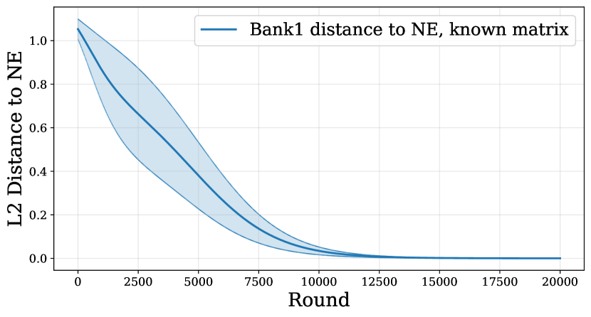
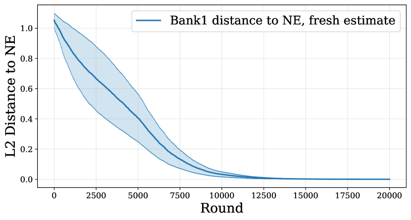
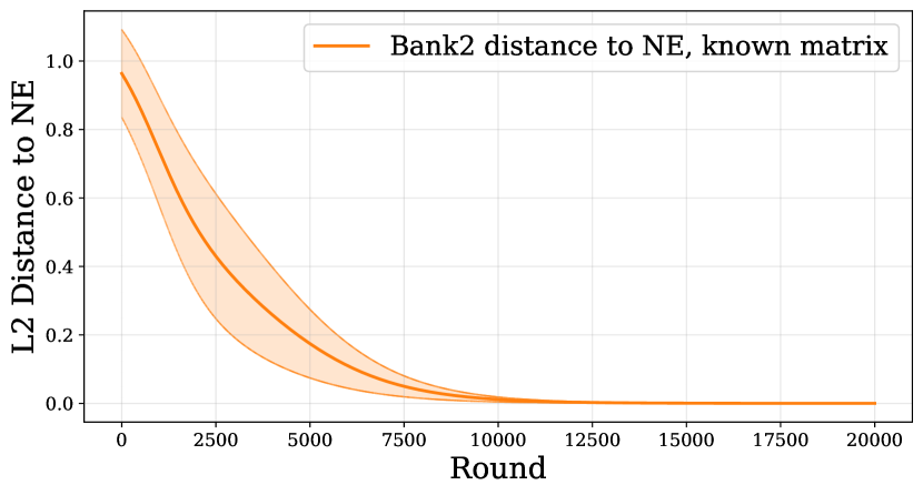
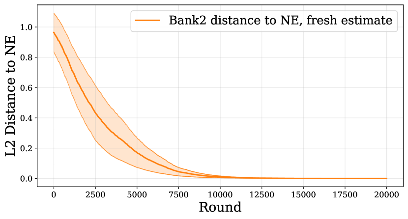
Figure 13: Case + + : Distance of the iterates of Bank1 (top row) and Bank2 (bottom row) to the Nash equilibrium. Left: known utility matrices. Right: estimated utilities using a single sample per round. $y\sim$ truncated Gaussian ($\mu=0.3,\sigma=0.1$), $\gamma_{l}=0.4$, $\gamma_{h}=0.8$. Mean(solid) and standard error (shaded) across 5 random initializations.

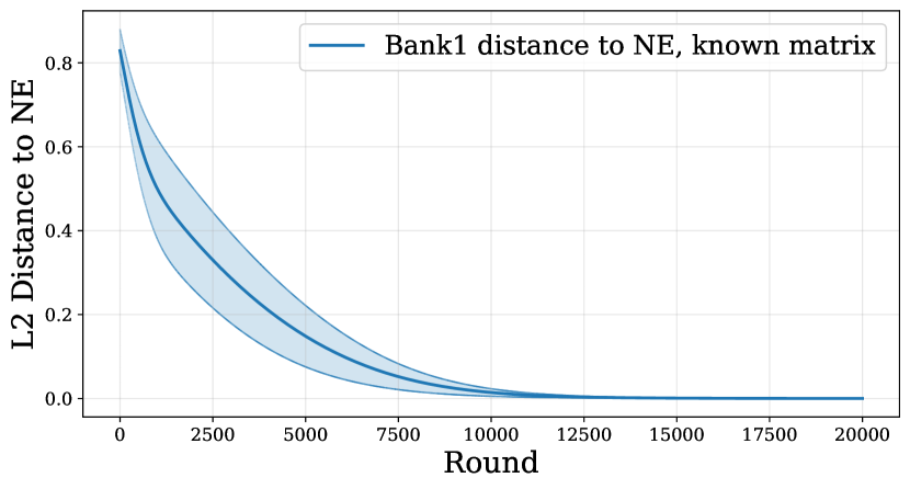
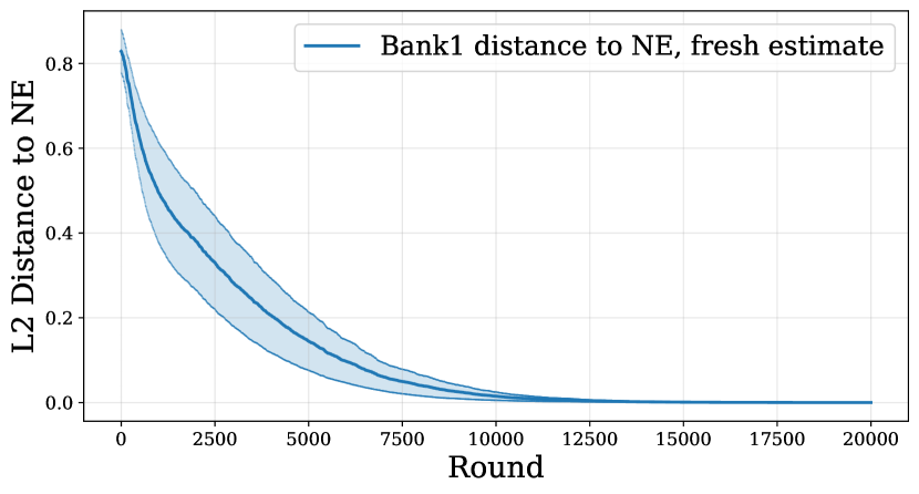
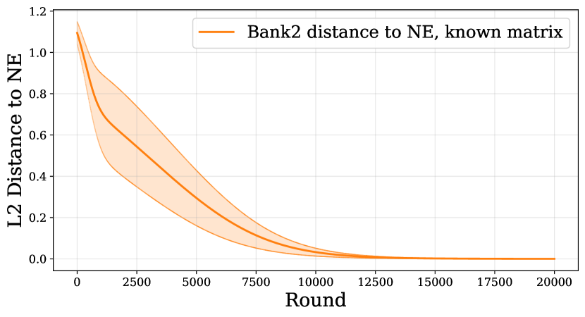
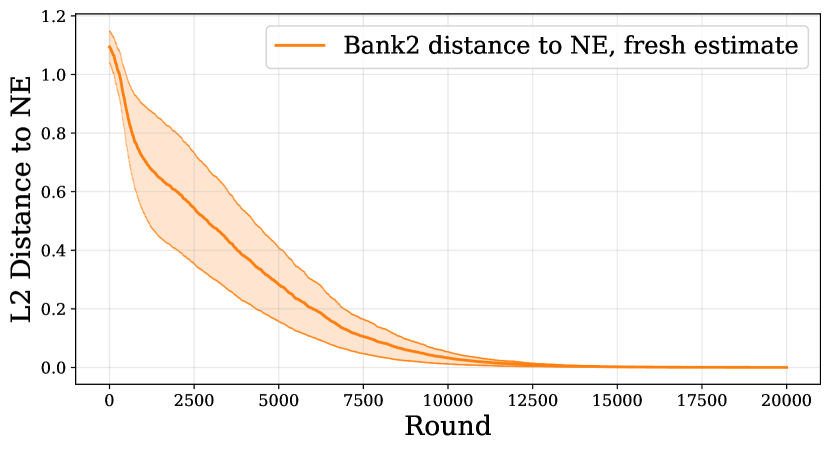
Figure 14: Case - -: Distance of the iterates of Bank1 (top row) and Bank2 (bottom row) to the Nash equilibrium. Left: known utility matrices. Right: estimated utilities using a single sample per round. $y\sim$ truncated Gaussian ($\mu=0.1,\sigma=0.3$), $\gamma_{l}=0.4$, $\gamma_{h}=0.8$. Mean(solid) and standard error (shaded) across 5 random initializations.

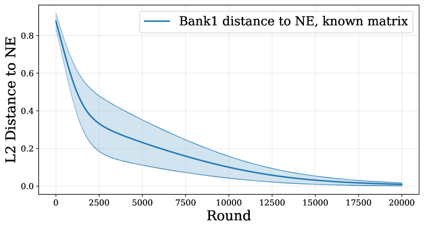
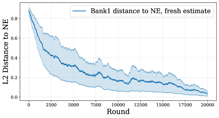
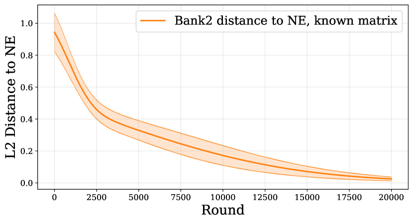
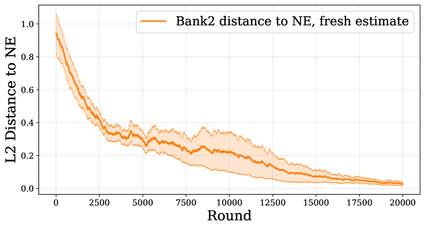
Figure 15: Case - +: Distance of the iterates of Bank1 (top row) and Bank2 (bottom row) to the Nash equilibrium. Left: known utility matrices. Right: estimated utilities using a single sample per round.$y$ follows a piecewise uniform distribution, $\gamma_{l}=0.6$, $\gamma_{h}=0.7$. Mean(solid) and standard error (shaded) across 5 random initializations.

Appendix F Representative Dynamics for the Bank Game with a Larger Action Set

 Input: step size $\eta>0$, time period $T$

 Initialization: $p_{1}^{(1)},p_{2}^{(1)}\in\Delta_{9}$

 for $t=1,\dots,T$ do

  Decision: Each player $i$ plays $\theta^{(j)}$ with probability $p_{i,j}^{(t)}$;

  Update Rule: Players update their probability distributions to $p_{1}^{(t+1)},~p_{2}^{(t+1)}$ as follows:

$$p^{(t+1)}_{1,j}\propto p^{(t)}_{1,j}\cdot\exp\left(\eta\sum_{k=1}^{9}p^{(t)}_{2,k}\cdot u_{1}\left(\theta^{(j)},\theta^{(k)}\right)\right),~~\forall k\in[9]$$

$$p^{(t+1)}_{2,j}\propto p^{(t)}_{2,j}\cdot\exp\left(\eta\sum_{k=1}^{9}p^{(t)}_{1,k}\cdot u_{2}\left(\theta^{(k)},\theta^{(j)}\right)\right),~~\forall k\in[9]$$

 end for

ALGORITHM 3 Online Learning Dynamic through Exponential Weights with Larger Decision Set

 Input: step size $\eta>0$, time period $T$, number of fresh samples at each round $n_{samples}$

 Initialization: $p_{1}^{(1)},p_{2}^{(1)}\in\Delta_{9}$

 for $t=1,\dots,T$ do

  Decision: Each player $i$ plays $\theta^{(j)}$ with probability $p_{i,j}^{(t)}$;

  Sampling: Sample a batch of customers $\mathcal{C}^{(t)}=\{y_{i}\}_{i=1}^{n_{samples}}$, where $y_{i}\sim\mathcal{D}_{y}$, for $i\in[n_{samples}]$

  Estimation: Construct Estimated Utility function $\widehat{u}_{1}(\theta_{1},\theta_{2},\mathcal{C}^{(t)})$ and $\widehat{u}_{2}(\theta_{1},\theta_{2},\mathcal{C}^{(t)})$ by (4.2) and (4.2).

  Update Rule: Players update their probability distributions to $p_{1}^{(t+1)},~p_{2}^{(t+1)}$ as follows:

$$p^{(t+1)}_{1,j}\propto p^{(t)}_{1,j}\cdot\exp\left(\eta\sum_{k=1}^{9}p^{(t)}_{2,k}\cdot\widehat{u}_{1}\left(\theta^{(j)},\theta^{(k)},\mathcal{C}^{(t)}\right)\right),~~\forall k\in[9]$$

$$p^{(t+1)}_{2,j}\propto p^{(t)}_{2,j}\cdot\exp\left(\eta\sum_{k=1}^{9}p^{(t)}_{1,k}\cdot\widehat{u}_{2}\left(\theta^{(k)},\theta^{(j)},\mathcal{C}^{(t)}\right)\right),~~\forall k\in[9]$$

 end for

ALGORITHM 4 Online Learning Dynamic through Exponential Weights with Fresh Samples and Larger Decision Set

In this section, we run the online learning dynamic with a larger action set. The deterministic version of the algorithm is given in Algorithm 3, and the stochastic version is in Algorithm 4. Specifically, we consider three interest rates: low, medium and high $\{\gamma_{l},\gamma_{m},\gamma_{h}\}$, along with the corresponding credit thresholds $\{\tau_{l}=\frac{1}{2+\gamma_{h}},\tau_{m}=\frac{1}{2+\gamma_{m}},\tau_{h}=\frac{1}{2+\gamma_{l}}\}$ Thus, the strategy for each bank is represented as a nine-dimensional vector in the probability simplex, $\Delta_{9}$, corresponding to the weight assignments on the following $9$ actions: $(\tau_{l},\gamma_{l}),(\tau_{l},\gamma_{m}),(\tau_{l},\gamma_{h}),(\tau_{m},\gamma_{l}),(\tau_{m},\gamma_{m}),(\tau_{m},\gamma_{h}),(\tau_{h},\gamma_{l}),(\tau_{h},\gamma_{m}),(\tau_{h},\gamma_{h}),$ and we enumerate them as $\{\theta^{(1)},\dots,\theta^{(9)}\}.$ In Appendix F.1, we provide figures for various Truncated Gaussian distributions, and in Appendix F.2, we present figures for different piecewise uniform distributions. The Nash equilibria for each instance are computed numerically using vertex enumeration [32].

We note here that the key insights from the two-interest-rate in the main body generally hold, with similar convergence of Algorithm 1 and 2 to Nash Equilibria. However, for carefully crafted piecewise uniform distributions, we observe cycling around the mixed Nash equilibrium. While rare, this phenomenon highlights that increasing the action space can, in specific cases, lead to non-convergent last iterates.

F.1 Game instances with Truncated Gaussian distributions

The instances of the Bank game with the truncated Gaussian distribution, along with their corresponding Nash equilibria and dynamics, are summarized in Table 3.

Distribution	$(\gamma_{l},\gamma_{m},\gamma_{h})$	Nash Equilibria	Figure
Truncated	$(0.1,0.4,0.8)$	1 pure:	Fig. 16
Gaussian $(0.3,0.1)$		$((\tau_{l},\gamma_{h}),(\tau_{l},\gamma_{h}))$
Truncated	$(0.1,0.4,0.8)$	1 pure:	Fig. 17
Gaussian $(0.1,0.3)$		$((\tau_{h},\gamma_{l}),(\tau_{h},\gamma_{l}))$
		2 symmetric mixed:	Fig. 18
		$\left(\begin{array}[]{c}(0,0,0.057,0,0,0,0.943,0,0),\\ (0,0,0.057,0,0,0,0.943,0,0)\end{array}\right)$
		$\left(\begin{array}[]{c}(0,0,0.319,0,0.16,0,0.521,0,0),\\ (0,0,0.319,0,0.16,0,0.521,0,0)\end{array}\right)$	Fig. 19
Truncated	$(0.1,0.4,0.8)$	2 pure:	Fig. 20,21
Gaussian $(0.1,0.2)$		$((\tau_{l},\gamma_{h}),(\tau_{l},\gamma_{h}))$
		$((\tau_{m},\gamma_{m}),(\tau_{m},\gamma_{m}))$
		1 symmetric mixed:	Fig. 22
		$\left(\begin{array}[]{c}(0,0,0.619,0,0.381,0,0,0,0),\\ (0,0,0.619,0,0.381,0,0,0,0)\end{array}\right)$

Table 3: Truncated Gaussian parameters, $3$ interest rates, Nash equilibria of the game, and figures for dynamics of Algorithm 3 and 4

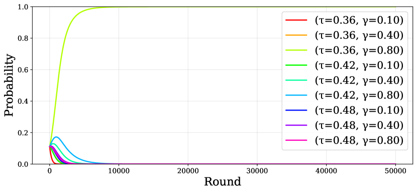
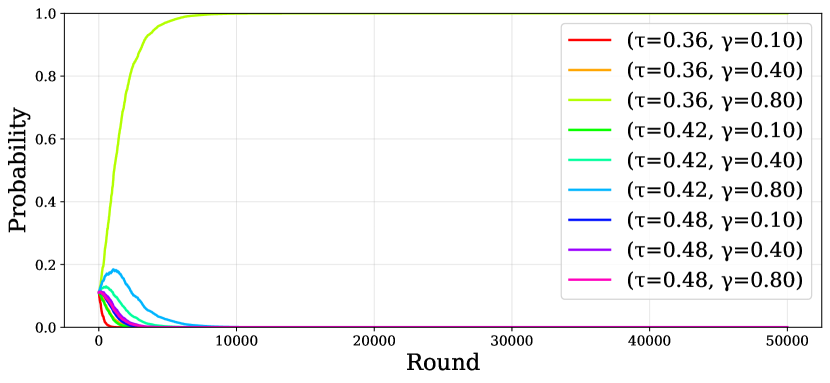
Figure 16: $y\sim$ Truncated Gaussian ($\mu=0.3,\sigma=0.1$), Exponential weights dynamics for Bank 1 (top row) and Bank 2 (bottom row), converging to the unique pure NE $((\tau_{l},\gamma_{h}),(\tau_{l},\gamma_{h}))$. Left: known utility matrices. Right: estimated utilities using a single sample per round. Initial weights for both banks are $(1/9\ldots 1/9)$

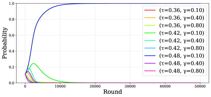
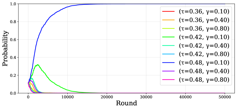
Figure 17: $y\sim$ Truncated Gaussian ($\mu=0.1,\sigma=0.3$), Exponential weights dynamics for Bank 1 (top row) and Bank 2 (bottom row), converging to the unique pure NE $((\tau_{h},\gamma_{l}),(\tau_{h},\gamma_{l}))$. Left: known utility matrices. Right: estimated utilities using a single sample per round. Initial weights for both banks are $(1/9\ldots 1/9)$

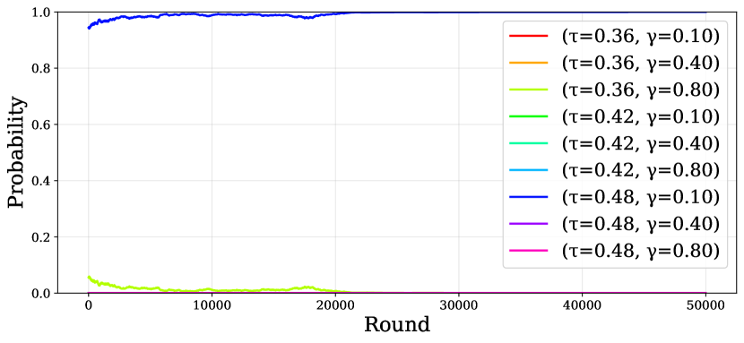
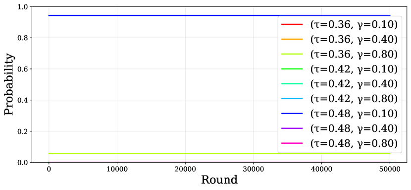
Figure 18: Truncated Gaussian ($\mu=0.1,\sigma=0.3$), Exponential weights dynamics for Bank 1 (top row) and Bank 2 (bottom row). Left: known utility matrices. Right: estimated utilities using a single sample per round. Both initialized at the mixed symmetric NE profile $(0,0,0.057,0,0,0,0.943,0,0)$. The dynamics with the known matrix are stationary at this NE, whereas those with the fresh estimate converge to the pure NE $((\tau_{h},\gamma_{l}),(\tau_{h},\gamma_{l}))$

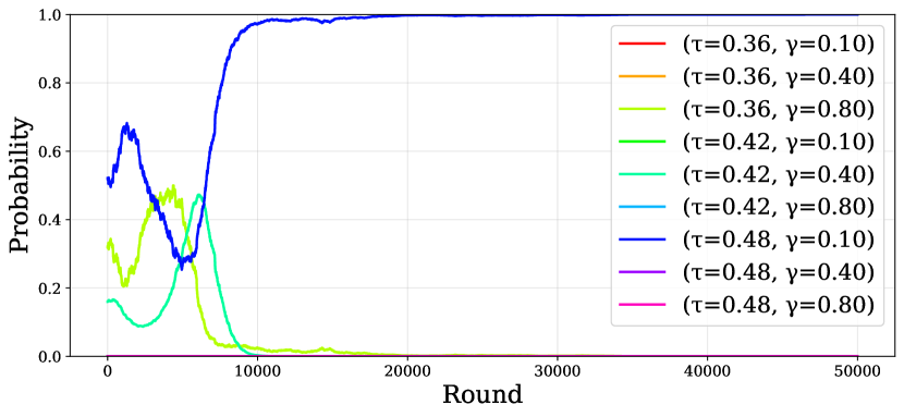
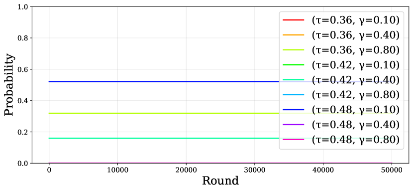
Figure 19: $y\sim$ Truncated Gaussian ($\mu=0.1,\sigma=0.3$), Exponential weights dynamics for Bank 1 (top row) and Bank 2 (bottom row). Left: known utility matrices. Right: estimated utilities using a single sample per round. Both banks initialized at the mixed symmetric NE profile $(0,0,0.319,0,0.16,0,0.521,0,0)$. The dynamics with the known matrix are stationary at this NE, whereas those with the fresh estimate converge to the pure NE $((\tau_{h},\gamma_{l}),(\tau_{h},\gamma_{l}))$

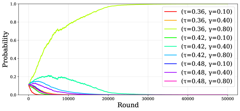
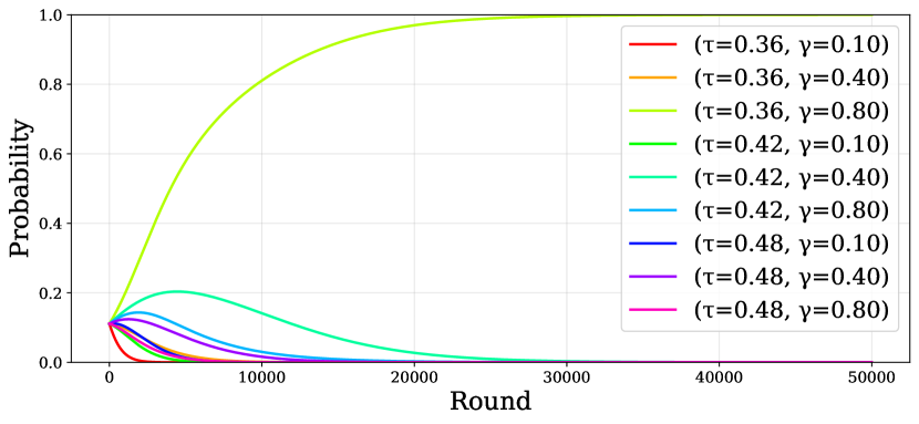
Figure 20: $y\sim$ Truncated Gaussian ($\mu=0.1,\sigma=0.2$), Exponential weights dynamics for Bank1 (top row) and Bank2 (bottom row), converging to the pure NE $((\tau_{l},\gamma_{h}),(\tau_{l},\gamma_{h}))$. Left: known utility matrices. Right: estimated utilities using a single sample per round. Initial weights for both banks are $(1/9\ldots 1/9)$

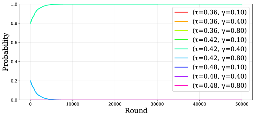
Figure 21: $y\sim$ Truncated Gaussian ($\mu=0.1,\sigma=0.2$), Exponential weights dynamics for Bank 1 (top row) and Bank 2 (bottom row), converging to the pure NE $((\tau_{m},\gamma_{m}),(\tau_{m},\gamma_{m}))$. Left: known utility matrices. Right: estimated utilities using a single sample per round. Initial weights for both banks are $(0,0,0,0,0.8,0.2,0,0,0)$

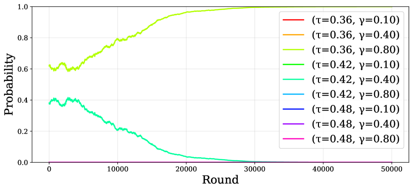
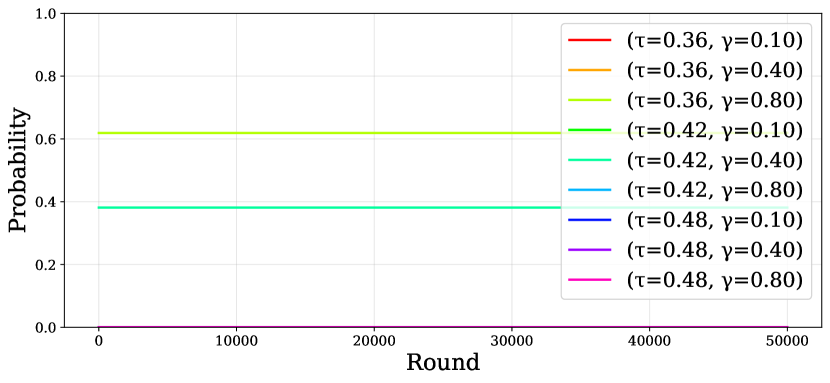
Figure 22: $y\sim$ Truncated Gaussian ($\mu=0.1,\sigma=0.2$), Exponential weights dynamics for Bank 1 (top row) and Bank 2 (bottom row). Left: known utility matrices. Right: estimated utilities using a single sample per round. Both banks initialized at the symmetric mixed NE profile $(0,0,0.619,0,0.381,0,0,0,0)$. The dynamics with the known matrix are stationary at this NE, whereas those with the fresh estimate converge to the pure NE $((\tau_{l},\gamma_{h}),(\tau_{l},\gamma_{h}))$

F.2 Game instances with piecewise uniform distributions

Most instances with piecewise uniform distributions and three interest rates converge to a Nash equilibrium. The instances in Table 4 are selected to highlight cases of non-convergence. The first instance has a unique symmetric mixed Nash equilibrium, with exponential weights dynamics cycling around it (Figure 23) for Algorithm 3 and 4. The second instance, which has two asymmetric and one symmetric mixed Nash equilibrium, shows cycling around the asymmetric mixed NE (Figure 24) and convergence to the symmetric mixed NE (Figure 25), depending on the initialization. While rare, these examples highlight that increasing the action space can, in certain cases, lead to non-convergent last iterates.

Distribution	$(\gamma_{l},\gamma_{m},\gamma_{h})$	Nash Equilibria	Figure
Piecewise	$(0.54,0.61,0.7)$	1 symmetric mixed:	Fig. 23
Uniform (Eq. (21))		$\left(\begin{array}[]{c}(0,0.395,0.32,0,0,0,0.286,0,0),\\ (0,0.395,0.32,0,0,0,0.286,0,0)\end{array}\right)$
Piecewise	$(0.77,0.81,0.93)$	2 asymmetric mixed:	Fig. 24
Uniform (Eq. (22))		$\left(\begin{array}[]{c}(0,0,0,0,0.315,0,0.685,0,0),\\ (0,0,0.851,0,0,0,0.149,0,0)\end{array}\right)$
		$\left(\begin{array}[]{c}(0,0,0.851,0,0,0,0.149,0,0),\\ (0,0,0,0,0.315,0,0.685,0,0)\end{array}\right)$
		1 symmetric mixed:	Fig. 25
		$\left(\begin{array}[]{c}(0,0,0.825,0,0,0,0.175,0,0),\\ (0,0,0.825,0,0,0,0.175,0,0)\end{array}\right)$

Table 4: Piecewise Uniform distributions, $3$ interest rates, Nash equilibria of the game, and figures for dynamics of Algorithm 1 and 2

Below, we provide the exact distribution for our two instances of the piecewise uniform distribution. Equation 21 corresponds to the case where $(\gamma_{l},\gamma_{m},\gamma_{h})=(0.54,0.61,0.7)$.

$$y\sim\begin{cases}0.01\times 2.61&y\in[0,\frac{1}{2.61}]\\ 0.95\times\frac{1}{(\frac{1}{2.54}-\frac{1}{2.61})},&y\in(\frac{1}{2.61},\frac{1}{2.54})\\ 0.04\times\frac{1}{(1-\frac{1}{2.54})}&y\in[\frac{1}{2.54},1]\end{cases}$$ (21)

Equation 22 corresponds to the case where $(\gamma_{l},\gamma_{m},\gamma_{h})=(0.77,0.81,0.93)$:

$$y\sim\begin{cases}0.01\times 2.93&y\in[0,\frac{1}{2.93}]\\ 0.95\times\frac{1}{(\frac{1}{2.77}-\frac{1}{2.93})},&y\in(\frac{1}{2.93},\frac{1}{2.77})\\ 0.04\times\frac{1}{(1-\frac{1}{2.77})}&y\in[\frac{1}{2.77},1]\end{cases}$$ (22)

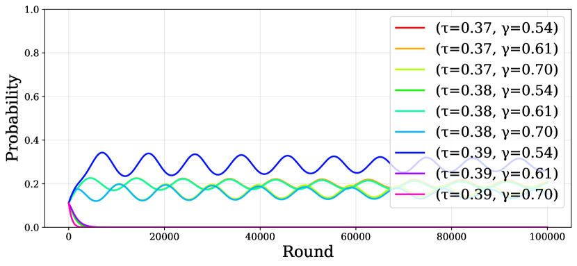
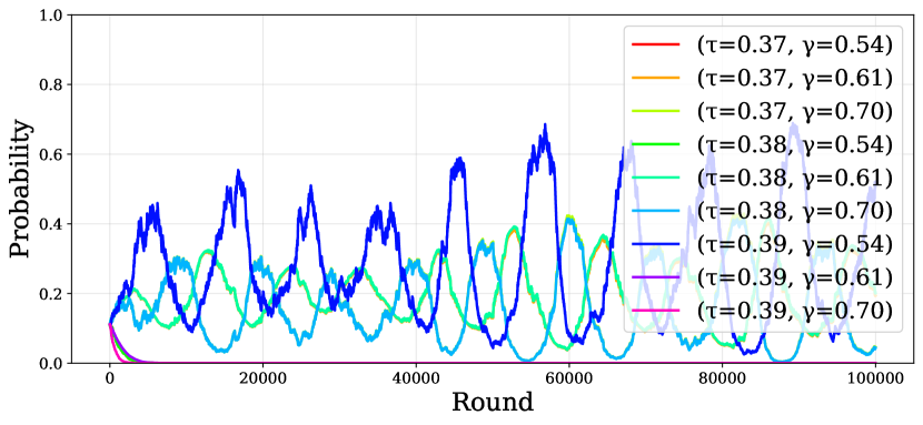
Figure 23: $y\sim$ Piecewise uniform (Eq(21)), Exponential weights dynamics for Bank 1 (top row) and Bank 2 (bottom row). Left: known utility matrices. Right: estimated utilities using a single sample per round. The banks are initialized at the mixed asymmetric Nash equilibrium $(1/9\ldots 1/9)$. The dynamics cycle around the mixed NE.

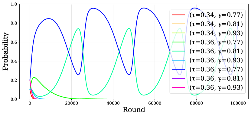
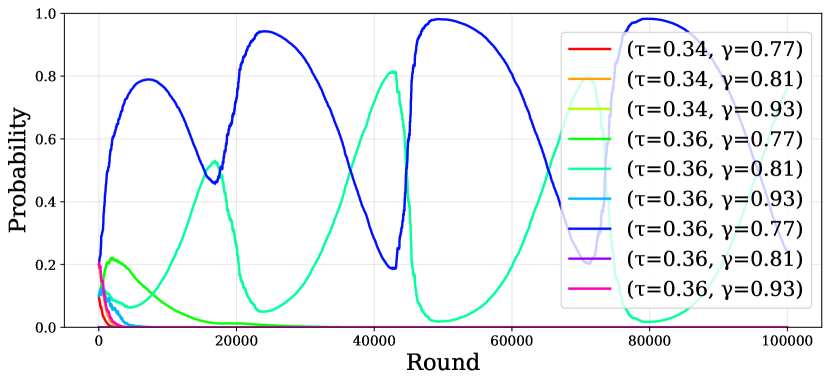
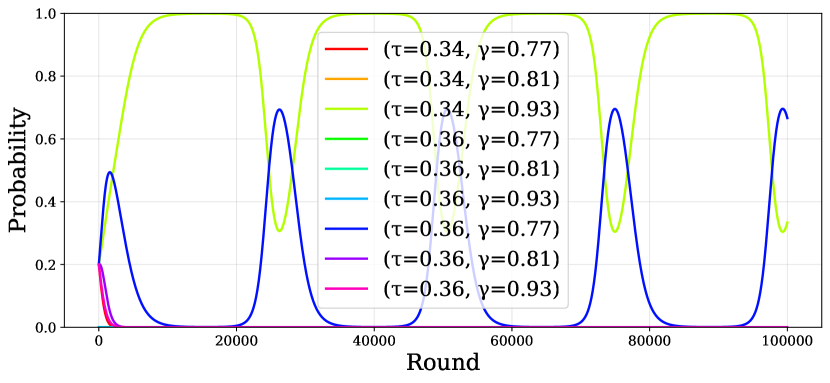
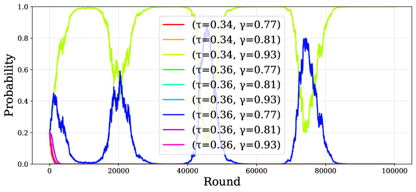
Figure 24: $y\sim$ Piecewise uniform (Eq(22)) Exponential weights dynamics for Bank 1 (top row) and Bank 2 (bottom row). Left: known utility matrices. Right: estimated utilities using a single sample per round, The banks are initialized at $((0.1,0.2,0.0,0.1,0.1,0.1,0.2,0,0.2),(0.2,0,0.2,0,0,0,0.2,0.2,0.2))$. The dynamics cycle around the asymmetric mixed Nash equilibrium

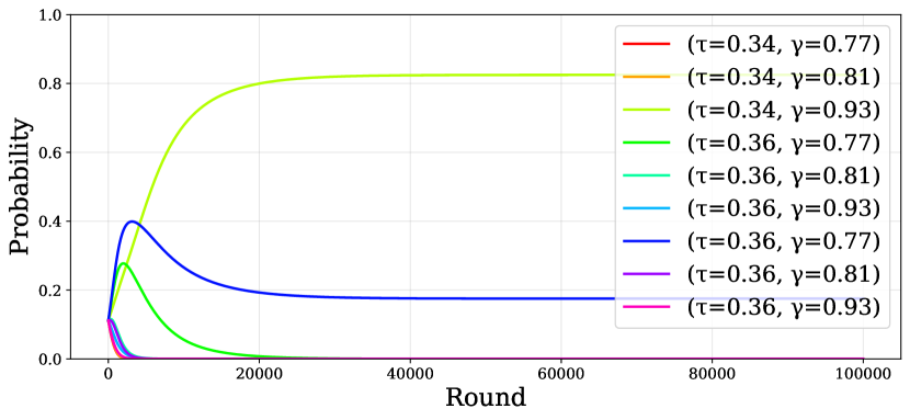
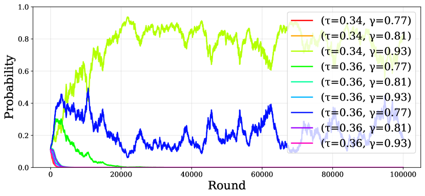
Figure 25: $y\sim$ Piecewise uniform (Eq(22)) Exponential weights dynamics for Bank 1 (top row) and Bank 2 (bottom row). Left: known utility matrices. Right: estimated utilities using a single sample per round, The banks are initialized at $(1/9\ldots 1/9)$. The dynamics converge to the symmetric mixed Nash equilibrium

References

- [1] Juan Perdomo, Tijana Zrnic, Celestine Mendler-Dünner, and Moritz Hardt. Performative prediction. In Proceedings of the 37th International Conference on Machine Learning, pages 7599–7609, 2020.
- [2] Celestine Mendler-Dünner, Juan Perdomo, Tijana Zrnic, and Moritz Hardt. Stochastic optimization for performative prediction. In H. Larochelle, M. Ranzato, R. Hadsell, M.F. Balcan, and H. Lin, editors, Advances in the 37th Neural Information Processing Systems, pages 4929–4939, 2020.
- [3] Gavin Brown, Shlomi Hod, and Iden Kalemaj. Performative prediction in a stateful world. In Proceedings of The 25th International Conference on Artificial Intelligence and Statistics, pages 6045–6061, 2022.
- [4] Yahav Bechavod, Katrina Ligett, Steven Wu, and Juba Ziani. Gaming helps! learning from strategic interactions in natural dynamics. In International Conference on Artificial Intelligence and Statistics, pages 1234–1242. PMLR, 2021.
- [5] Yonadav Shavit, Benjamin Edelman, and Brian Axelrod. Causal strategic linear regression. In International Conference on Machine Learning, pages 8676–8686. PMLR, 2020.
- [6] Celestine Mendler-Dünner, Juan Perdomo, Tijana Zrnic, and Moritz Hardt. Stochastic optimization for performative prediction. Advances in Neural Information Processing Systems, 33:4929–4939, 2020.
- [7] Moritz Hardt, Meena Jagadeesan, and Celestine Mendler-Dünner. Performative power. Advances in Neural Information Processing Systems, 35:22969–22981, 2022.
- [8] Moritz Hardt and Celestine Mendler-Dünner. Performative prediction: Past and future. arXiv preprint arXiv:2310.16608, 2023.
- [9] Sarah Dean, Mihaela Curmei, Lillian J Ratliff, Jamie Morgenstern, and Maryam Fazel. Multi-learner risk reduction under endogenous participation dynamics. arXiv e-prints, pages arXiv–2206, 2022.
- [10] Adhyyan Narang, Evan Faulkner, Dmitriy Drusvyatskiy, Maryam Fazel, and Lillian J Ratliff. Multiplayer performative prediction: Learning in decision-dependent games. Journal of Machine Learning Research, 24(202):1–56, 2023.
- [11] Michael Brückner and Tobias Scheffer. Stackelberg games for adversarial prediction problems. In Proceedings of the 17th ACM SIGKDD international conference on Knowledge discovery and data mining, pages 547–555, 2011.
- [12] Moritz Hardt, Nimrod Megiddo, Christos Papadimitriou, and Mary Wootters. Strategic classification. In Proceedings of the 2016 ACM conference on innovations in theoretical computer science, pages 111–122, 2016.
- [13] Meena Jagadeesan, Celestine Mendler-Dünner, and Moritz Hardt. Alternative microfoundations for strategic classification. In International Conference on Machine Learning, pages 4687–4697. PMLR, 2021.
- [14] Ganesh Ghalme, Vineet Nair, Itay Eilat, Inbal Talgam-Cohen, and Nir Rosenfeld. Strategic classification in the dark. In International Conference on Machine Learning, pages 3672–3681. PMLR, 2021.
- [15] Yahav Bechavod, Chara Podimata, Steven Wu, and Juba Ziani. Information discrepancy in strategic learning. In International Conference on Machine Learning (ICML), pages 1691–1715, 2022.
- [16] Nika Haghtalab, Chara Podimata, and Kunhe Yang. Calibrated stackelberg games: Learning optimal commitments against calibrated agents. Advances in Neural Information Processing Systems, 36, 2023.
- [17] Lee Cohen, Saeed Sharifi-Malvajerdi, Kevin Stangl, Ali Vakilian, and Juba Ziani. Sequential strategic screening. In International Conference on Machine Learning, pages 6279–6295. PMLR, 2023.
- [18] Yeshwanth Cherapanamjeri, Constantinos Daskalakis, Andrew Ilyas, and Manolis Zampetakis. What makes a good fisherman? linear regression under self-selection bias. In Proceedings of the 55th Annual ACM Symposium on Theory of Computing, pages 1699–1712, 2023.
- [19] Guy Horowitz, Yonatan Sommer, Moran Koren, and Nir Rosenfeld. Classification under strategic self-selection. arXiv preprint arXiv:2402.15274, 2024.
- [20] Jason Gaitonde and Elchanan Mossel. Sample-efficient linear regression with self-selection bias. arXiv preprint arXiv:2402.14229, 2024.
- [21] Manolis Zampetakis. Analyzing data with systematic bias. ACM SIGecom Exchanges, 20(1):55–63, 2022.
- [22] Pang Wei Koh, Shiori Sagawa, Henrik Marklund, Sang Michael Xie, Marvin Zhang, Akshay Balsubramani, Weihua Hu, Michihiro Yasunaga, Richard Lanas Phillips, Irena Gao, et al. Wilds: A benchmark of in-the-wild distribution shifts. In International conference on machine learning, pages 5637–5664. PMLR, 2021.
- [23] Yoav Freund and Robert E Schapire. Adaptive game playing using multiplicative weights. Games and Economic Behavior, 29(1-2):79–103, 1999.
- [24] Sergiu Hart. Adaptive heuristics. Econometrica, 73(5):1401–1430, 2005.
- [25] Sergiu Hart and Andreu Mas-Colell. Uncoupled dynamics do not lead to nash equilibrium. American Economic Review, 93(5):1830–1836, 2003.
- [26] Constantinos Daskalakis and Ioannis Panageas. Last-iterate convergence: Zero-sum games and constrained min-max optimization. In 10th Innovations in Theoretical Computer Science Conference (ITCS 2019). Schloss-Dagstuhl-Leibniz Zentrum für Informatik, 2019.
- [27] Yang Cai, Argyris Oikonomou, and Weiqiang Zheng. Finite-time last-iterate convergence for learning in multi-player games. Advances in Neural Information Processing Systems, 35:33904–33919, 2022.
- [28] Emmanouil-Vasileios Vlatakis-Gkaragkounis, Lampros Flokas, Thanasis Lianeas, Panayotis Mertikopoulos, and Georgios Piliouras. No-regret learning and mixed nash equilibria: They do not mix. Advances in Neural Information Processing Systems, 33:1380–1391, 2020.
- [29] Angeliki Giannou, Emmanouil Vasileios Vlatakis-Gkaragkounis, and Panayotis Mertikopoulos. Survival of the strictest: Stable and unstable equilibria under regularized learning with partial information. In Conference on Learning Theory, pages 2147–2148. PMLR, 2021.
- [30] V Vovk. A game of prediction with expert advice. Journal of Computer and System Sciences, 56(2):153–173, 1998.
- [31] Nick Littlestone and Manfred K. Warmuth. The weighted majority algorithm. Information and Computation, 108(2):212–261, 1994.
- [32] Tim Roughgarden. Algorithmic game theory. Communications of the ACM, 53(7):78–86, 2010.