Scale Setting and Strong Coupling Determination in the Gradient Flow Scheme for 2+1 Flavor Lattice QCD

Abstract

We report on a scale determination, scale setting, and determination of the strong coupling in the gradient flow scheme using the $N_{f}=2+1$ highly improved staggered quark (HISQ) ensembles generated by the HotQCD Collaboration for bare gauge couplings ranging from $\beta=7.030$ to $8.400$. The gradient flow scales we obtain in this work are $\sqrt{t_{0}}=0.14229(98)$ fm and $w_{0}=0.17190(140)$ fm. Using the decay constants of the kaon and $\eta_{s}$, as well as the bottomonium mass splitting from the literature, we also calculate the potential scale $r_{1}$, obtaining $r_{1}=0.3072(22)$ fm. We fit the flow scales to an Allton-type ansatz as a function of $\beta$, providing a polynomial expression that allows for the prediction of lattice spacings at new $beta$ values. As a secondary result, we make an attempt to determine $\Lambda_{\overline{\mathrm{MS}}}$ and use it to estimate the strong coupling in the $\overline{\mathrm{MS}}$ scheme.

I Introduction

Scale setting is an essential step in the lattice calculations that converts the lattice computed dimensionless quantity to dimensionful quantity in physical units. It affects the accuracy of lattice calculations in such a fundamental way that it must be handled as precisely as possible. There are different strategies to this end, which roughly divide into two categories. One is to use the physical scales that are experimentally accessible, the other is to use the theory scales. The former mainly includes the mass of baryons (e.g. $\Omega$) [1, 2, 3, 4, 5] and the pion/kaon decay constant $f_{\pi}$/$f_{K}$, see, e.g. [1, 4, 5, 6]. The latter mainly includes the (static-quark) potential scales $r_{0}$ and $r_{1}$ [7, 8, 9, 10, 11, 12], the fictitious pseudoscalar decay constant $F_{p4s}$ [13, 14], and the gradient flow scales $t_{0}$ and $w_{0}$ [2, 3, 15, 16, 14, 17, 3, 10, 1, 18, 19] which we will pursue in this work. Since the theory scales have no direct physical implications, they must be pegged to those physical scales in practical implementation. In principle, any dimensionful quantity can be used to “define” a theory scale, as long as it is finite in the continuum limit. But in practice it is only worth to consider those that are cheap and straightforward to compute on the lattice. That is, these quantities must be precise enough that with a small computational cost one can acquire good control on the statistical and systematic uncertainties.

Among them are the commonly used potential scales $r_{0}$ and $r_{1}$ proposed two decades ago [7, 8]. They are defined by $r^{2}\mathrm{d}V(r)/\mathrm{d}r=1.65$ or $1$ for $r=r_{0}$ or $r_{1}$, respectively. Usually the potential $V(r)$ itself is precise on the lattice, but when the lattice is very fine, the statistical uncertainties of the Wilson loops at large temporal distances (in lattice units) become significant, which weakens the control of the excited-state contamination. $F_{p4s}$, on the other hand, has a relatively strong dependence on the valence quark mass by definition, and the asymptotic fits needed to extract $f_{p4s}$ are usually challenging [13].

Gradient flow [20, 21] is a seminal framework that has applications in many fields, such as renormalization, defining operators, noise reduction, scale setting, $et\ al$. The flow scales are introduced based on a crucial property of gradient flow that any operator comprised of the flowed gauge fields renormalizes only through the renormalization of the gauge coupling [22]. Thus a scale can be defined (at a certain flow time) when setting the composite operator to a predefined physical value. For gradient flow scales the relevant composite operator is the vacuum gauge action density $E$. The flow scales have been a topic of intense study for the last decade for their stability and high precision. This is due to the fact that the action density is very precise on the lattice and no asymptotic fits are needed to obtain the scales. In several recent studies, the calculations have been pushed to 2+1+1 flavor lattice QCD using different actions, and the obtained results can reach sub-percent level precision, see [15, 2, 14, 3, 18] for a selection. Such calculations can mostly be extrapolated to the continuum limit and the physical pion mass limit.

In this work, we compute $t_{0}$ and $w_{0}$ on the 2+1 flavor highly improved staggered quark (HISQ) ensembles generated by the HotQCD Collaboration in [10, 23, 24] at large $\beta$ values. We use Symanzik improved gradient flow [25, 26] and action density discretized using both standard clovers and $\mathcal{O}(a^{2})$-improved field strength tensor. The obtained flow scales serve as an alternative to the potential scales, and are more accurate. This will shed light on a better understanding of the systematic uncertainties in the scale setting. Besides the scale setting, we also make an attempt to determine the $\Lambda_{\overline{\mathrm{MS}}}$ parameter using the matching relation between the gradient flow scheme and the $\overline{\text{MS}}$ scheme [27, 28]. $\Lambda_{\overline{\mathrm{MS}}}$ plays a crucial role in QCD theory. It predicts the energy dependence of the running coupling constant $\alpha_{\overline{\mathrm{MS}}}$ and signals the nonperturbative effects in the theory. However, determining $\Lambda_{\overline{\mathrm{MS}}}$ from lattice QCD is intractable. Typically, one needs to compute a “measure” in lattice QCD and fit it to its perturbative counterpart expanded in $\alpha_{\overline{\mathrm{MS}}}$ that involves $\Lambda_{\overline{\mathrm{MS}}}$. However, the logarithmic terms appearing at high orders render the convergence of the perturbative series questionable. This issue presents itself as the main difficulty in such studies that limits the accuracy of the extracted $\Lambda_{\overline{\mathrm{MS}}}$ parameter [29, 30, 31]. We will discuss this in more detail later.

This paper is organized as follows. We start with a short summary of the theoretical foundations, including the gradient flow equations, the definitions of the gradient flow scales $t_{0}$ and $w_{0}$ and the Allton-type ansatz that relates the flow scales to $\beta$ in Sec. II. In Sec. III.1 we provide the lattice setup used in this study. In Sec. III.2 we present our results for the flow scales, the comparisons of the ratios of scales with the literature and the relation that determines the lattice spacing $a$ given $\beta$ via flow scales. In Sec. IV we present the results for the flow scales and potential scales in physical units. In Sec. V we show how to calculate $\Lambda_{\overline{\mathrm{MS}}}$ using gradient flow. We summarize our findings in Sec. VI.

II Formalism

Yang-Mills gradient flow evolves the gauge fields along the gradient of the gauge action according to the following diffusion equation [20, 21]

$$B_{\mu}(x,\tau_{\mathrm{F}}=0) =A_{\mu}(x),$$ (1)

$$\partial_{\tau_{\mathrm{F}}}B_{\mu}(x,\tau_{\mathrm{F}}) =D_{\nu}G_{\nu\mu},$$ (2)

where $A_{\mu}(x)$ is the original gauge field and $B_{\mu}(x,\tau_{\mathrm{F}})$ denotes the gauge field flowed to flow time $\tau_{\mathrm{F}}$. $D_{\nu}$ and $G_{\mu}(x)$ are the flowed covariant derivative and field strength constructed using $B_{\mu}(x,\tau_{\mathrm{F}})$. On the lattice the flow equations take the form

$$V(x,\mu)|_{\tau_{\mathrm{F}}=0} =U(x,\mu),$$ (3)

$$\frac{\mathrm{d}}{\mathrm{d}\tau_{\mathrm{F}}}V(x,\mu) =-g_{0}^{2}\{\partial_{x,\mu}S_{G}(V)\}V(x,\mu),$$ (4)

where $U(x,\mu)$ is the original gauge link and $V(x,\mu)$ is its flowed version. $g_{0}$ is the bare coupling and $S_{G}$ can take different forms upon how the gauge action is discretized. In this work we use the Zeuthen flow [32] that adopts a Symanzik improved L$\ddot{\mathrm{u}}$scher–Weisz gauge action [25, 26] eliminating all the $\mathcal{O}(a^{2})$ discretization effects.

The (leading order) solutions of the flow equations Eq. (1) are related by a $\tau_{\mathrm{F}}$ dependent transformation of the field $B_{\mu}(x,\tau_{\mathrm{F}})$ [33]

$$\begin{split}&B_{\mu}(x,\tau_{\mathrm{F}})=\int\mathrm{d}^{4}y\ K_{\tau_{\mathrm{F}}}(x-y)A_{\mu}(y),\\ &K_{\tau_{\mathrm{F}}}(z)=\int\frac{\mathrm{d}^{4}p}{(2\pi)^{4}}e^{ipz}e^{-\tau_{\mathrm{F}}p^{2}}=\frac{e^{-z^{2}/4\tau_{\mathrm{F}}}}{(4\pi\tau_{\mathrm{F}})^{2}},\end{split}$$ (5)

via a local Gaussian smearing kernel $K_{\tau_{\mathrm{F}}}$ with radius $\sqrt{8\tau_{\mathrm{F}}}$ [22]. The smearing removes the short-distance fluctuations of the gauge fields and has been widely used as a noise reduction technique, see e.g. [34, 35, 36, 37]. In this work we use it to define non-perturbative reference scales, which involve a very simple gauge invariant operator–the action density, that reads

$$E(\tau_{\mathrm{F}},x)=-\frac{1}{2}\mathrm{Tr}\{G_{\mu\nu}(\tau_{\mathrm{F}},x)G_{\mu\nu}(\tau_{\mathrm{F}},x)\}.$$ (6)

In practical simulations an average over all space-time position $x$ is taken.

The gradient flow scales $t_{i}$ and $w_{i}$ can be defined by imposing the conditions [33, 3]

$$\begin{split}\tau_{\mathrm{F}}^{2}\langle E(\tau_{\mathrm{F}})\rangle\Big{|}_{\tau_{\mathrm{F}}=t_{i}}&=c_{i},\\ \tau_{\mathrm{F}}\frac{\mathrm{d}}{\mathrm{d}\tau_{\mathrm{F}}}\left\{\tau_{\mathrm{F}}^{2}\langle E(\tau_{\mathrm{F}})\rangle\right\}\Big{|}_{\tau_{\mathrm{F}}=w_{i}^{2}}&=c_{i},i=0,1,2.\end{split}$$ (7)

The commonly used choice $c_{0}=0.3$ defines the scales $t_{0}$ and $w_{0}$ that are often used in the lattice calculations. The alternative choice $c_{1}=0.7$ has been used by Wuppertal-Budapest Collaboration to define $w_{1}$ scale [38]. In this work we also consider the choice $c_{2}=0.2$ that defines scales $t_{2}$ and $w_{2}$. Note that in lattice calculations all quantities are in lattice units, thus what one can obtain from these two conditions are actually two dimensionless quantities $\sqrt{t_{i}}/a$ and $w_{i}/a$. In this study, we consider two different discretizations for the action density $E$, in terms of two different discretization for the field strength tensor $F_{\mu\nu}$. One is to use the clover-type discretization

$$\hat{F}^{\mathrm{clo}}_{\mu\nu}(n)=-\frac{i}{8}\Big{(}Q_{\mu\nu}(n)-Q_{\nu\mu}(n)\Big{)},$$ (8)

where $Q_{\mu\nu}(n)$ is sum of four square plaquettes, see, e.g. [39]. The operator is hatted to indicate that it is in lattice units. The other is based on an $a^{2}$-improved discretization that employs a mixture of square and $1\times 2$ rectangle plaquettes

$$\hat{F}^{\mathrm{imp}}_{\mu\nu}(n)=\frac{5}{3}C^{(1,1)}_{\mu\nu}(n)-\frac{1}{3}C^{(1,2)}_{\mu\nu}(n),$$ (9)

see [40] for more details. Comparing the results from the two discretizations we can learn how large the discretization effects are in the calculations.

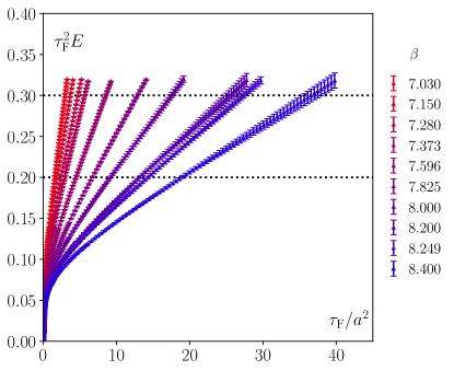
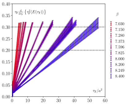
Figure 1: Numerical results for the action density, $E$ (left) and the derivative of $\tau_{F}^{2}E$(right) as function of the flow time obtained using the improved discretization.

Once the flow scales are obtained, they are fit to the following Allton-type Ansatz [41] as a function of $\beta$,

$$\begin{split}&\ln\left(\frac{\sqrt{t_{i}}}{a}\right)=\frac{1+d_{2i}(10/\beta)f^{2}(\beta)}{c_{0i}f(\beta)+c_{2i}(10/\beta)f^{3}(\beta)},\\ &\ln\left(\frac{w_{i}}{a}\right)=\frac{1+d^{\prime}_{2i}(10/\beta)f^{2}(\beta)}{c^{\prime}_{0i}f(\beta)+c^{\prime}_{2i}(10/\beta)f^{3}(\beta)},\\ &f(\beta)=\left(\frac{10b_{0}}{\beta}\right)^{-b_{1}/(2b_{0}^{2})}\exp(-\beta/(20b_{0})),\\ \end{split}$$ (10)

where $\beta=10/g_{0}^{2}$, $b_{0}=9/(4\pi)^{2}$ and $b_{1}=1/(4\pi^{4})$ for $N_{f}=3$. ($d_{2i}$, $c_{0i}$, $c_{2i}$) and ($d^{\prime}_{2i}$, $c^{\prime}_{0i}$, $c^{\prime}_{2i}$) are fit parameters. Using $t_{0}$ and $w_{0}$ in physical units obtained through $f_{K}$ and $f_{\eta_{s}}$ (which we will return to in Sec.IV), the lattice spacing can be predicted for new $\beta$.

III Gradient flow scales in 2+1 flavor lattice QCD

III.1 Lattice setup

$\beta$	$am_{s}$	$am_{l}$	$N_{\sigma}$	$N_{\tau}$	# conf.
7.030	0.0356	0.00178	48	48	900
7.150	0.0320	0.00160	48	64	395
7.280	0.0280	0.00142	48	64	398
7.373	0.0250	0.00125	48	64	554
7.596	0.0202	0.00101	64	64	577
7.825	0.0164	0.0082	64	64	471
8.000	0.01299	0.002598	64	64	1004
8.200	0.01071	0.002142	64	64	961
8.249	0.01011	0.002022	64	64	2241
8.400	0.00887	0.001774	64	64	2372

Table 1: Parameters of the lattice ensembles used in this work, including the inverse gauge coupling $\beta=10/g_{0}^{2}$, the bare quark masses in lattice units, the spatial and temporal lattice extent $N_{\sigma}$ and $N_{\tau}$, and the corresponding number of configurations.

The calculations are carried out on the ensembles generated by the HotQCD Collaboration in [10, 23, 24] using 2+1 flavor HISQ action [42] and tree-level improved L$\ddot{\mathrm{u}}$scher-Weisz gauge action [25, 26]. Ten large $\beta$ values are employed ranging from 7.030 to 8.400 in this study. The details are summarized in Tab.1. In all cases, the strange quark mass $m_{s}$ is tuned to match the mass of the fictitious unmixed pseudo scalar meson $\eta_{s}$ to 695 MeV, close to its physical value 685.8 MeV. The light quarks are degenerate $m_{u}=m_{d}=m_{l}$. In the first block of Tab.1 ($7.03\leq\beta\leq 7.825$), the light quark masses are fixed as a fraction of the strange quark mass $m_{s}/m_{l}=20$, slightly above the physical ratio $m_{s}/m_{l}=27.3$. This corresponds to a pion mass of about 160 MeV in the continuum limit. In the second block ($8.000\leq\beta\leq 8.400$) the light quark mass is even larger and follows $m_{s}/m_{l}=5$, corresponding to a pion mass of around 320 MeV. In all cases, the temporal extents are chosen such that the corresponding temperatures are well below the crossover temperature to eliminate the thermal effects. The ensembles at different $\beta$ values enable us to perform the continuum extrapolation that is almost a must have in such studies nowadays. It is worth mentioning that not all ensembles are used in every analysis. In individual analyses we select different ensembles based on necessity. We want to stress that, while the action density is stable and precise on the lattice, the auto-correlation in it is typically strong, especially at large flow times. Thus a careful error analysis is necessary. The details of the error analysis are provided in Appendix A.

$\beta$	7.03	7.15	7.28	7.373	7.596	7.825	8.000	8.200	8.249	8.400
$\sqrt{t_{0}}/a$(clover)	1.8259(5)	2.0217(8)	2.2636(13)	2.4549(19)	2.9847(28)	3.634(9)	4.228(33)	5.083(79)	5.262(50)	6.076(108)
$\sqrt{t_{0}}/a$(impr.)	1.7298(5)	1.9334(7)	2.1831(13)	2.3799(19)	2.9218(30)	3.586(7)	4.184(33)	5.044(78)	5.225(50)	6.045(106)
$\sqrt{t_{2}}/a$(clover)	1.3891(2)	1.5276(4)	1.6076(5)	1.8320(7)	2.2048(12)	2.669(3)	3.096(12)	3.688(21)	3.837(26)	4.399(32)
$\sqrt{t_{2}}/a$(impr.)	1.2593(2)	1.4056(3)	1.5841(4)	1.7244(7)	2.1116(12)	2.591(3)	3.027(11)	3.629(20)	3.780(25)	4.347(29)
$w_{0}/a$(clover)	2.0730(13)	2.3159(21)	2.6203(36)	2.8575(48)	3.5194(73)	4.292(24)	4.978(83)	6.156(345)	6.233(81)	7.293(330)
$w_{0}/a$(impr.)	2.0674(13)	2.3121(22)	2.6178(37)	2.8558(50)	3.5193(72)	4.304(19)	4.978(83)	6.156(345)	6.233(81)	7.297(333)
$w_{2}/a$(clover)	1.6832(8)	1.8826(13)	2.1302(15)	2.3258(27)	2.8653(40)	3.510(13)	4.083(47)	4.999(188)	5.109(60)	5.954(199)
$w_{2}/a$(impr.)	1.6883(8)	1.8893(14)	2.1380(16)	2.3341(27)	2.8740(44)	3.524(11)	4.089(47)	5.006(189)	5.115(60)	5.962(201)

Table 2: The dimensionless flow scales $\sqrt{t_{i}}/a$ and $w_{i}/a$ determined from different discretization at different $\beta$.

$\sqrt{t_{0}}/a$(clover)	$c_{00}$	$c_{20}$	$d_{20}$	$c_{m0}$	$\chi^{2}$/d.o.f.
	87.012(1792)	10807220(4152523)	110183(43757)	-0.1891(1515)	1.9
$w_{0}/a$(clover)	$c^{\prime}_{00}$	$c^{\prime}_{20}$	$d^{\prime}_{20}$	$c^{\prime}_{m0}$	$\chi^{2}$/d.o.f.
	73.757(1098)	2431121(869632)	26488(10950)	-0.6947(4230)	1.5
$\sqrt{t_{2}}/a$(clover)	$c_{02}$	$c_{22}$	$d_{22}$	$c_{m2}$	$\chi^{2}$/d.o.f.
	3.4646$\times 10^{-6}$ ( 2.242$\times 10^{-5}$)	1094905782(143539661)	8372082(1119049)	0.6219(416)	15.5
$w_{2}/a$(clover)	$c^{\prime}_{02}$	$c^{\prime}_{22}$	$d^{\prime}_{22}$	$c^{\prime}_{m2}$	$\chi^{2}$/d.o.f.
	90.125(1032)	2983654(697943)	26136 (7223)	-0.5124(2947)	1.3
$\sqrt{t_{0}}/a$(impr.)	$c_{00}$	$c_{20}$	$d_{20}$	$c_{m0}$	$\chi^{2}$/d.o.f.
	89.531 (627)	2622963(439476)	233936(4462)	-0.2419(1739)	0.8
$w_{0}/a$(impr.)	$c^{\prime}_{00}$	$c^{\prime}_{20}$	$d^{\prime}_{20}$	$c^{\prime}_{m0}$	$\chi^{2}$/d.o.f.
	73.891(972)	2123699(642507)	22715(7796)	-0.5048(3382)	1.4
$\sqrt{t_{2}}/a$(impr.)	$c_{02}$	$c_{22}$	$d_{22}$	$c_{m2}$	$\chi^{2}$/d.o.f.
	124.776(501)	3770654(344897)	24658(2499)	-0.1307(971)	1.5
$w_{2}/a$(impr.)	$c^{\prime}_{02}$	$c^{\prime}_{22}$	$d^{\prime}_{22}$	$c^{\prime}_{m2}$	$\chi^{2}$/d.o.f.
	90.501(914)	2494878(576243)	2.1574(5579)	-0.3905(2408)	1.2

Table 3: Fit parameters of the flow scales to the Allton Ansatz.

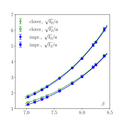
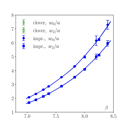
Figure 2: The gradient flow scales $t_{i}$ (left) and $w_{i}$ (right) as function of $\beta$. The lines represent the fits to Allton Ansatz.

III.2 Determination of the gradient flow scales

$\beta$	7.03	7.15	7.28	7.373	7.596	7.825
$a^{2}/w_{0}^{2}$(clover)	0.2327	0.1864	0.1456	0.1225	0.0807	0.0543
$a^{2}/w_{0}^{2}$(impr.)	0.2339	0.1871	0.1459	0.1226	0.0807	0.0540

Table 4: The values of $a^{2}/w_{0}^{2}$ in the clover and improved discretization respectively.

	$\sqrt{t_{0}}/w_{0}$	$\sqrt{t_{2}}/w_{2}$	$\sqrt{t_{0}}/\sqrt{t_{2}}$	$w_{0}/w_{2}$
	$a^{2}$	$a^{2}$	$a^{2}$	$a^{2}$
6 largest $\beta$	0.8337(19), 1.3	0.7426(15), 2.6	1.3717(10), 4.9	1.2256(20), 1.4
5 largest $\beta$	0.8307(28), 1.0	0.7382(20), 1.1	1.3762(14), 1.6	1.2244(28), 1.5
4 largest $\beta$	0.8318(44), 1.0	0.7357(32), 0.8	1.3799(22), 0.5	1.2202(40), 1.1
3 largest $\beta$	0.8331(49), 0.9	0.7369(38), 0.5	1.3792(27), 0.3	1.2194(47), 1.0

	$\sqrt{t_{0}}/w_{0}$			$\sqrt{t_{2}}/w_{2}$
	$a^{2}$	$a^{4}$	$\alpha_{b}a^{2}$	$a^{2}$	$a^{4}$	$\alpha_{b}a^{2}$
6 largest $\beta$	0.8286(20), 1.0	0.8315(13), 1.2	0.8293(19), 1.1	0.7285(13), 1.3	0.7345(9), 1.8	0.7299(13), 1.3
5 largest $\beta$	0.8262(32), 0.9	0.8296(20), 0.8	0.8269(30), 0.9	0.7264(19), 1.2	0.7325(11), 1.0	0.7277(18), 1.1
4 largest $\beta$	0.8276(47), 1.0	0.8295(28), 0.9	0.8280(43), 1.0	0.7274(37), 1.4	0.7311(22), 0.9	0.7282(34), 1.3
3 largest $\beta$	0.8291(64), 1.1	0.8301(40), 1.1	0.8293(59), 1.1	0.7311(40), 0.5	0.7331(27), 0.4	0.7316(37), 0.4
	$\sqrt{t_{0}}/\sqrt{t_{2}}$			$w_{0}/w_{2}$
	$a^{2}$	$a^{4}$	$\alpha_{b}a^{2}$	$a^{2}$	$a^{4}$	$\alpha_{b}a^{2}$
6 largest $\beta$	1.3888(11), 1.9	1.3834(7), 3.4	1.3876(11), 2.1	1.2235(22), 1.0	1.2238(14), 1.0	1.2236(20), 1.0
5 largest $\beta$	1.3906(17), 1.5	1.3854(10), 1.5	1.3894(15), 1.5	1.2241(33), 1.0	1.2243(20), 1.0	1.2242(30), 1.0
4 largest $\beta$	1.3907(26), 1.8	1.3870(17), 1.1	1.3899(23), 1.7	1.2220(46), 0.9	1.2229(28), 1.0	1.2222(41), 1.0
3 largest $\beta$	1.3880(32), 0.6	1.3859(22), 0.4	1.3875(30), 0.5	1.2236(69), 1.1	1.2240(40), 1.1	1.2237(62), 1.1

Table 5: Continuum-extrapolated ratios of the flow scales from different fit strategies using data from the clover (top) and improved discretization (middle and bottom). The numbers are in the form {Mean(Error), $\chi^{2}$/d.o.f.}.

We determined the gradient flow scales $t_{i}$ and $w_{i}$, $i=0,2$ through Eq. (7) using clover or improved discretization for the action density. The numerical results for the action density, $E$ and the derivative $\tau_{F}E$ as function of the flow time are shown in Fig. 1 for improved discretizations. The results for clover discretization look similar. We interpolate the numerical results on the action density in flow time using splines to determine its derivative. From the splines it is straightforward to evaluate the gradient flow scales. Our results for the gradient flow scales in lattice units are shown in Fig. 2 and also summarized in Table 2. From Fig. 2 we see that there are some differences in the $t_{0}/a$ values obtained with clover discretization and improved discretization at smaller values of $\beta$. However, for $w_{0}/a$ scale these differences are smaller. The $t_{2}$ and $w_{2}$ scales have smaller statistical errors compared to $t_{0}$ and $w_{0}$ scales, which is advantageous for large values of $\beta$. At the same time differences between the results obtained with clover and improved discretizations are larger for $t_{2}$ and $w_{2}$.

We performed Allton fits of the gradient flow scales. To account for the mass discrepancy, we modify the Allton Ansatz Eq. (10) by multiplying a correction factor $1+c_{mi}(am_{s}+2am_{l})$ with $c_{mi}$ being an additional fit parameter. Then the $m_{s}/20$ and $m_{s}/5$ data can be fit jointly, using the bare quark masses in lattice units $am_{l}$, $am_{s}$ listed in Table 1 as inputs. The fits are shown in Fig. 2, in which the curves are calculated using interpolated bare masses and obtained fit parameters, which are summarized in Table 3. We find that in all cases the Allton Ansatz can describe the data well except for $\sqrt{t_{2}}/a$ from clover discretization, which can be attributed to the fact that the statistical errors for this scale are extraordinary small, while the systematic errors from lattice cutoff effects can be much larger than them but are not included in the fits.

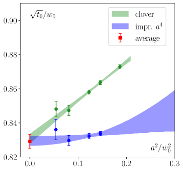
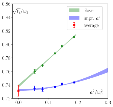
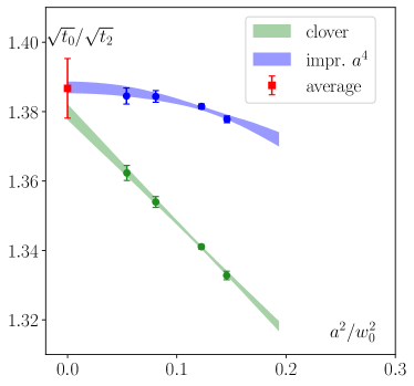
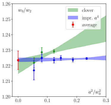
Figure 3: The ratio of different gradient flow scale as function of the lattice spacing together with the continuum extrapolations. The flow scales are measured using both the clover discretizations and the improved discretization (labelled as “clover” and “impr.”, respectively, see Eq. (8)-Eq. (9)). In these plots only the “best” fits are shown which correspond to the numbers in bold in Table 5.

Next we determine the ratio of different gradient flow scales: $\sqrt{t_{0}}/w_{0}$, $\sqrt{t_{2}}/w_{2}$, $\sqrt{t_{0}}/\sqrt{t_{2}}$ and $w_{0}/w_{2}$ using lattices at 7.030$\leq\beta\leq$ 7.825 listed in the first block of Table 1. The values of $a^{2}/w_{0}^{2}$ in the clover and improved discretization respectively for these lattices are summarized in Table 4. Since these scales are measured on the same ensembles, correlations naturally exist between them. To account for these correlations, we compute each scale separately using the same bootstrap samples. Additionally, there are autocorrelations among the measured scales. These are addressed by binning the data with a bin size equal to twice the integrated autocorrelation time, $\tau_{\mathrm{int}}$, prior to bootstrapping. Here, $\tau_{\mathrm{int}}$ is taken as the larger value from the numerator or denominator that form the ratio. These ratios are shown in Fig. 3 as function of the lattice spacing in units of $w_{0}$ for a few selected $\beta$s that can produce good fits. For clover discretization we expect that these ratios scale as $a^{2}$. For improved discretization we expect the lattice spacing dependence to be proportional to either $a^{4}$ or $\alpha_{s}a^{2}$. We see that indeed the $a^{2}$ dependence of these ratios is much reduced compared to clover discretization. We performed continuum extrapolations of these ratios which are shown as bands in Fig. 3. For clover discretization we performed $a^{2}$ extrapolations, while for improved discretization we also performed $\alpha_{b}a^{2}$ and $a^{4}$ extrapolations, with $\alpha_{b}$ being the boosted lattice gauge coupling $\alpha_{b}=g_{0}^{2}/(4\pi u_{0}^{4})=10/(4\pi\beta u_{0}^{4})$. Here $u_{0}^{4}$ stands for the average plaquette taken from [29]. For the improved discretization we also consider the $a^{2}$ extrapolations as an effective description of the $\alpha_{b}a^{2}$ extrapolations. The continuum-extrapolated ratios show visible discrepancy when using different fit Ansatz in most cases for the improved discretization. Besides, there also exists non-negligible difference between the clover discretization and the improved discretization. To examine the systematic uncertainties stemming from these aspects, we perform the continuum extrapolations by excluding different number of coarser lattices. The fit results are summarized in Table 5. We can see that some of the fits can be identified as good while some can not. To pick out the good fits we adopt the following criteria i) $\chi^{2}/$d.o.f. should be the closest to 1.0 (keeping one decimal place); ii) if there are two such fits, we take the one that has more number of data points. The selected best fits are in bold in Table 5. Performing a weighted average of the selected best fits and assigning the maximal deviation between the average and the selected values as the systematic uncertainty we obtain

$$\begin{split}\sqrt{t_{0}}/w_{0}&=0.8292(26)(15),\\ \sqrt{t_{2}}/w_{2}&=0.7314(15)(67),\\ \sqrt{t_{0}}/\sqrt{t_{2}}&=1.3867(18)(68),\\ w_{0}/w_{2}&=1.2235(19)(41),\end{split}$$ (11)

where the first numbers in the parenthesis denote the statistical uncertainties while the second ones the systematic uncertainties. The averaged results are shown as red data points in Fig. 3, with the error bar being the sum of the statistical uncertainties and the systematic uncertainties. The obtained $\sqrt{t_{0}}/w_{0}$ is consistent with the $N_{f}$=2+1+1 estimate from EMT Collaboration [15] 0.82930(65) and the $N_{f}$=2+1+1 estimate from HPQCD Collaboration [18] 0.835(8).

III.3 The relation of the gradient flow scales to the potential scales

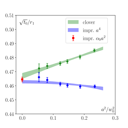
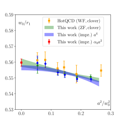
Figure 4: Continuum extrapolation of the ratio of the flow scales to the $r_{1}$ scale. Left: $\sqrt{t_{0}}/r_{1}$. Similar to before, the discretization effects are significant in this case. After applying the $\mathcal{O}(a^{2})$ improvement to the field strength tensor, the slope of the extrapolation (using Ansatz linear in $a^{2}$) changes sign. However, in the continuum limit, the two discretizations give consistent results. Right: $w_{0}/r_{1}$. “WF” stands for Wilson flow and “ZF” for Zeuthen flow. We include results from the HotQCD Collaboration (red points) [10] using Wilson flow and clover-discretized action density for comparison. It can be observed that for $w_{0}$, the discretization effects are so mild that the two discretizations give almost the same results. Our results using Zeuthen flow are slightly smaller than the HotQCD Collaboration’s previous results using Wilson flow.

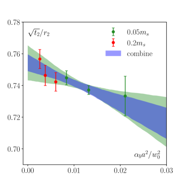
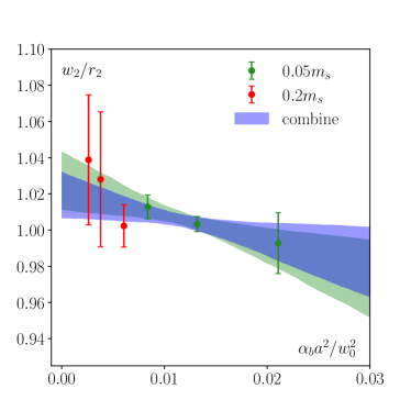
Figure 5: The ratio of the gradient flow slales $\sqrt{t_{2}}$ and $w_{2}$ to $r_{2}$ scale as function of the lattice spacing.

As mentioned in the introduction theoretical scales based on the static quark anti-quark potential, $V(r)$ are often used in lattice QCD calculations. These scales are defined as

$$\left.r^{2}\frac{dV(r)}{dr}\right|_{r=r_{i}}=b_{i},~i=0,1,2.$$ (12)

The choices $b_{0}=1.65$, $b_{1}=1$ and $b_{2}=1/2$ define the $r_{0}$ (Sommer) [7], $r_{1}$ scale [8] and $r_{2}$ scale [23], respectively. In this subsection we express the gradient flow scales in terms of $r_{1}$ and $r_{2}$ scales. Since the discretization effects in the static potential are expected to be small at distances around $r_{1}$ and $r_{2}$ the ratio of the gradient flow scales and the potential scales can give some insight into the lattice artifacts in the determination of the gradient flow scales. Based on the lattices listed in the first block of Table 1, our result for the ratios $r_{1}/\sqrt{t_{0}}$ and $r_{1}/w_{0}$ are shown in Fig. 4. For the latter we compare our results with the results of HotQCD Collaboration [10] obtained using Wilson flow and clover-discretized action density for comparison. Our results agree with the HotQCD results within errors. As one can see from the figure for $r_{1}/\sqrt{t_{0}}$ improved discretization scheme leads to much smaller cutoff effects. On the other hand for $r_{1}/w_{0}$ there is no visible difference between the two discretization schemes and also Wilson flow leads to similar to similar results. This suggest that lattice artifacts are smaller in the $w_{0}$ scale compared to the $t_{0}$ scale. We performed continuum extrapolations for $r_{1}/\sqrt{t_{0}}$ and $r_{1}/w_{0}$ for both clover and improved discretization assuming $a^{2}$-dependence. For improved action density we also performed $\alpha_{b}a^{2}$ and $a^{4}$ extrapolations. All the continuum extrapolations of these ratios agree within the estimated errors, see c.f. Fig. 4. Using improved action density and $\alpha_{b}a^{2}$ extrapolation we obtain:

$$r_{1}/\sqrt{t_{0}}=2.1530(78),~r_{1}/w_{0}=1.7866(74).$$ (13)

Our result for $r_{1}/w_{0}$ could be compared with HotQCD result, $r_{1}/w_{0}=1.7797(67)$ for $N_{f}=2+1$ [10] and the HPQCD result, $r_{1}/w_{0}=1.789(26)$ for $N_{f}=2+1+1$ [18]. We see that all results for $r_{1}/w_{0}$ agree within errors. Recently the $r_{1}/a$ scale has been determined in 2+1+1 flavor QCD using HISQ action by TUMQCD collaboration for large range of lattice spacing down to $a=0.032$ fm [12]. Using these values of $r_{1}/a$ as well as the 2+1+1 flavor HISQ results for $\sqrt{t_{0}}/a$ and $w_{0}/a$ [14, 43] we estimated the continuum values of and $r_{1}/\sqrt{t_{0}}$ and $r_{1}/w_{0}$ assuming discretization effects scale as $\alpha_{b}a^{2}$. We obtain:

$$r_{1}/\sqrt{t_{0}}=2.1601(83),~r_{1}/w_{0}=1.7749(96),~N_{f}=2+1+1,$$ (14)

which agree well with our 2+1 flavor results above. From the recent TUMQCD results we know that the $r_{1}$ scale is not affected by the charm quark mass because at distances $r>0.2$ fm charm quarks do not change the shape of the potential [12]. Therefore, the above result implies that the values of $t_{0}$ and $w_{0}$ are also not affected by the dynamical charm effects.

In Fig. 5 we show the ratio of the gradient flow scales $\sqrt{t_{2}}$ and $w_{2}$ to $r_{2}$. The $r_{2}/a$ data is taken from [23], available for the lattices at $\beta=$7.373, 7.596, 7.825, 8.000, 8.200 and 8.400. The light quark mass effects in this ratio appear to be quite small. We performed continuum extrapolations for these ratios using $\alpha_{b}a^{2}$ form. These continuum extrapolations are shown in Fig. 5 both including and excluding results for $m_{l}=m_{s}/5$. Using all the available data we obtain:

$$\sqrt{t_{2}}/r_{2}=0.7544(52),~w_{2}/r_{2}=1.0265(142).$$ (15)

Excluding the $m_{s}/5$ data does not change the above result but only increases the errors slightly.

IV Gradient flow scales in physical units

In order to obtain the values of the gradient flow scales in physical units one calculates the dimensionless product of these scales and some physical energy scales, like the meson decay constants or mass differences of different quarkonium states at different lattice spacing and extrapolates these to the continuum limit. Using the values of these quantities from experiments one finally gets the gradient flow scale in physical units. Below we will discuss the determination of the gradient flow scales from meson decay constant and bottomonium splitting.

IV.1 Determination of the scales theory scales from decay constants

We will use the kaon decay constant, $f_{K}$ and the decay constant of unmixed pseudo-scalar $s\bar{s}$ meson, $f_{\eta_{s}}$ to obtain the values of the gradient flow scale in physical units. The latter cannot be determined experimentally as there is no unmixed pseudo-scalar $s\bar{s}$ meson, but the corresponding decay constant can be related to pion and kaon decay constant using chiral perturbation theory [6]. We will use the values of $af_{K}$ and $af_{\eta_{s}}$ obtained by HotQCD Collaboration in 2+1 flavor QCD for light quark masses $m_{l}=m_{s}/20$ with $m_{s}$ being the strange quark mass [10]. Since the HotQCD calculations have been performed at slightly larger than the physical light quark masses ($m_{s}/20$ instead of $m_{s}/27$), and also the strange quark mass is slightly different from the physical strange quark mass [10], it is important to correct the decay constants for the mass effects. This can be done by using leading-order (LO) chiral perturbation theory, which suggests a general relation between the quark mass and the decay constant of the corresponding meson, $f_{\mathrm{meson}}=f_{0}+s\cdot(m_{1}+m_{2})$, where $m_{1}$ and $m_{2}$ are the masses of the quarks that form the meson, and $f_{0}$ is the decay constant for massless quarks. Here, $s$ represents the slope that needs to be determined. For kaon and $\eta_{s}$ we can write two equations explicitly as follows

$$\begin{split}af^{\mathrm{meas}}_{{\eta_{s}}}&=af_{0}+2s\cdot am^{\mathrm{input}}_{s},\\ af^{\mathrm{meas}}_{K}&=af_{0}+s(am^{\mathrm{input}}_{l}+am^{\mathrm{input}}_{s}).\end{split}$$ (16)

Using the values of $af^{\mathrm{meas}}_{K}$, $af^{\mathrm{meas}}_{\eta_{s}}$ obtained in [10] and the input bare quark masses that satisfy $am^{\mathrm{input}}_{s}/am^{\mathrm{input}}_{l}=20$, we determine the slope $s$. We use this slope in the following equations to calculate the decay constants in the physical point

$$\begin{split}af_{\eta_{s}}^{\mathrm{phys}}(\beta)&=af_{\eta_{s}}^{\mathrm{meas}}(\beta)+2s\cdot\Big{(}am_{s}^{\mathrm{LCP}}(\beta)\left(\frac{m_{{\eta_{s}}}^{\mathrm{phys}}}{m_{{\eta_{s}}}^{\mathrm{LCP}}}\right)^{2}\\ &-am_{s}^{\mathrm{input}}(\beta)\Big{)},\\ af_{K}^{\mathrm{phys}}(\beta)&=af_{K}^{\mathrm{meas}}(\beta)+s\cdot\Big{(}am_{s}^{\mathrm{LCP}}(\beta)\left(\frac{m_{{\eta_{s}}}^{\mathrm{phys}}}{m_{{\eta_{s}}}^{\mathrm{LCP}}}\right)^{2}\\ f&\times\frac{28.3}{27.3}-am_{s}^{\mathrm{input}}(\beta)\cdot\frac{21}{20}\Big{)}.\end{split}$$ (17)

Here $m_{s}^{LCP}$ stands for the strange quark mass along the lines of constant physics (LCP), which in Ref. [10] was fixed by requiring that the mass of the unmixed pseudo-scalar $s\bar{s}$ meson is constant a $m_{\eta_{s}}^{\mathrm{LCP}}$=695 MeV , and $m_{{\eta_{s}}}^{\mathrm{phys}}=685.8$ MeV is its physical value [6]. A few remarks are needed to better understand how we arrive at these two equations. First, we can write two equations similar as Eq. (16) for the physical decay constants and physical quark masses. We then subtract off Eq. (16) from them and write the physical strange quark mass as

$$m_{s}^{\mathrm{phys}}(\beta)=m_{s}^{\mathrm{LCP}}(\beta)\cdot\left(\frac{m_{\eta_{s}}^{\mathrm{phys}}}{m_{\eta_{s}}^{\mathrm{LCP}}},\right)^{2}.$$ (18)

The ratios $28.3/27.3$ and $21/20$ in the above equation emerge as a consequence of the relation between the physical strange quark mass and light quark mass, which is $m_{s}^{\mathrm{phys}}/m_{l}^{\mathrm{phys}}=27.3$, and the relation for the bare masses, which is $m_{s}^{\mathrm{input}}/m_{l}^{\mathrm{input}}=20$. The strange quark mass along the LCP, $m_{s}^{\mathrm{LCP}}(\beta)$, can be calculated using the following parametrization [10]

$$\begin{split}&\frac{r_{1}}{a}\cdot am_{s}^{\mathrm{LCP}}=\frac{r_{1}}{a}\cdot am^{\mathrm{RGI}}\left(\frac{20b_{0}}{\beta}\right)^{4/9}\times\\ &\ \ \ \frac{1+m_{1}\frac{10}{\beta}f^{2}(\beta)+m_{2}(\frac{10}{\beta})^{2}f^{2}(\beta)+m_{3}\frac{10}{\beta}f^{4}(\beta)}{1+dm_{1}\frac{10}{\beta}f^{2}(\beta)}\;,\end{split}$$ (19)

where $f(\beta)$ is given in Eq. (10). $r_{1}/a$, $am^{\mathrm{RGI}}$, $m_{1}$, $m_{2}$, $m_{3}$ and $dm_{1}$ can be found in [10]. We note that for these mass corrections we always employ Gaussian bootstrap. The errors of the quantities taken from [10], including $af^{\mathrm{meas}}_{K}$, $af^{\mathrm{meas}}_{{\eta_{s}}}$, $r_{1}/a$ and $m^{\mathrm{RGI}}$, enter the fit as (inverse) weights. For $m_{1}$, $m_{2}$, $m_{3}$ and $dm_{1}$ the errors are omitted as they are strongly correlated and Gaussian bootstrap essentially ignores all the correlation. The obtained Gaussian bootstrap samples of the decay constants are multiplied by the bootstrap samples of the flow scales, and the resultant products are shown as data points in Fig.6. Performing continuum extrapolation of them gives the continuum values listed in Table 6.

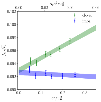
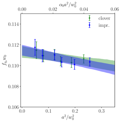
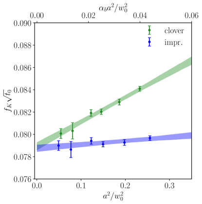
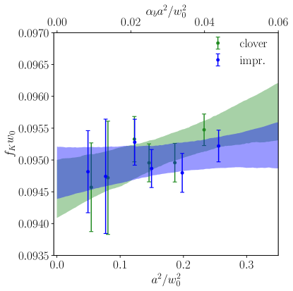
Figure 6: Continuum extrapolation (bands) of the products (points) of the flow scales and the decay constants. Top left: $f_{\eta_{s}}\sqrt{t_{0}}$. Top right: $f_{\eta_{s}}w_{0}$. Bottom left: $f_{K}\sqrt{t_{0}}$. Bottom right: $f_{K}w_{0}$. It can be seen that the discretization effects are significant for $\sqrt{t_{0}}$, and are strongly suppressed when applying the $\mathcal{O}(a^{2})$ improvement, while for $w_{0}$ the discretization effects are very mild at these $\beta$ values. The data from clover discretization are continuum-extrapolated using a $a^{2}$ model lying along the first $x$-axis labeled $a^{2}/w_{0}$ while the data from improved discretization are continuum-extrapolated using a $\alpha_{b}a^{2}$ model lying along the second $x$-axis labeled $\alpha_{b}a^{2}/w_{0}$. After continuum extrapolation two discretizations give consistent results in all cases, demonstrating that the discretization effects and lattice cutoff effects are completely under control.

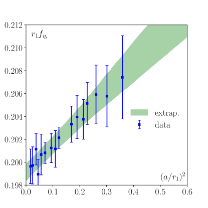
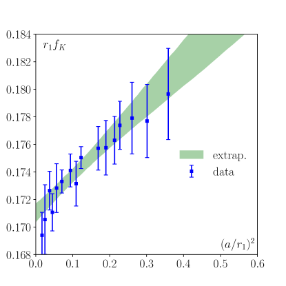
Figure 7: Continuum extrapolation (band, labelled as “extrap.”) of $r_{1}f_{\eta_{s}}$ (left) and $r_{1}f_{K}$ (right) based on the data of $r_{1}/a$, $af_{\eta_{s}}$ and $af_{K}$ taken from [10].

	$f^{\mathrm{meas}}_{{\eta_{s}}}\sqrt{t_{0}}\times 100$	$f^{\mathrm{meas}}_{{\eta_{s}}}w_{0}\times 100$	$f^{\mathrm{meas}}_{K}\sqrt{t_{0}}\times 100$	$f^{\mathrm{meas}}_{K}w_{0}\times 100$	$r_{1}/\sqrt{t_{0}}$	$r_{1}/w_{0}$
clover	9.292(44)	11.132(56)	7.893(36)	9.455(45)	2.1530(78)	1.7866(74)
impr.	9.261(42)	11.148(52)	7.876(32)	9.480(41)	2.1506(86)	1.7835(80)

Table 6: The continuum-extrapolated values of $f^{\mathrm{meas}}_{{\eta_{s}}}\sqrt{t_{0}}$, $f^{\mathrm{meas}}_{{\eta_{s}}}w_{0}$, $f^{\mathrm{meas}}_{K}\sqrt{t_{0}}$, $f^{\mathrm{meas}}_{K}w_{0}$, $r_{1}/\sqrt{t_{0}}$ and $r_{1}/w_{0}$.

The results elucidate that $\sqrt{t_{0}}$ is sensitive to how the action density is discretized, while $w_{0}$ is not. After improvement, $\sqrt{t_{0}}$ becomes almost free from the cutoff effects. The products are extrapolated to the continuum limit using an Ansatz linear in $a^{2}$. We find that this Ansatz can describe our data points in all cases. The $\chi^{2}$/d.o.f. is 1.1, 0.9, 1.0 and 1.0 for $f_{\eta_{s}}\sqrt{t_{0}}$, $f_{\eta_{s}}w_{0}$, $f_{K}\sqrt{t_{0}}$ and $f_{K}w_{0}$, respectively. Note that these results are for the improved action density operator, continuum-extrapolated using $\alpha_{b}a^{2}$ model. We provide results only for this operator here, and later, if not particularly specified, as it has a better control over the discretization error. The consistency of results from different discretizations in the continuum limit suggests that the discretization errors and lattice cutoff effects are well controlled. Using the values of the decay constants $f_{\eta_{s}}=$ 128.34(85) MeV [6] and $f_{K}$ = 110.10(64) MeV [10] for $t_{0}$ scale we find

$$\begin{split}\sqrt{t_{0}}&=0.14239(65)(94)~{\rm fm}~{\rm via}~f_{\eta_{s}},\\ \sqrt{t_{0}}&=0.14133(57)(82)~{\rm fm}~{\rm via}~f_{K},\\ \end{split}$$ (20)

while for $w_{0}$ scale we find

$$\begin{split}w_{0}&=0.17139(80)(113)~{\rm fm},~{\rm via}~f_{\eta_{s}},\\ w_{0}&=0.17012(74)(98)~{\rm fm},~{\rm via}~f_{K}.\\ \end{split}$$ (21)

The first error in the above equations stands for the statistical error, while the second errors represents the error propagated from the cited decay constants. We see that the values of the gradient flow scales determined from $f_{\eta_{s}}$ and $f_{K}$ are consistent within errors. The above results based on the decay constants are smaller than the FLAG average [44, 45]. Using the value of the ratio $r_{1}/\sqrt{t_{0}}$ and $r_{1}/w_{0}$ given in Eq. (13), we find

$$\begin{split}r_{1}&=0.3053(37)\ \mathrm{fm\ via}\ \sqrt{t_{0}},\\ r_{1}&=0.3050(38)\ \mathrm{fm\ via}\ w_{0}.\\ \end{split}$$ (22)

Obviously, $r_{1}$ can be determined directly through the decay constants $f_{\eta_{s}}$ and $f_{K}$. We revisit this calculation by taking the $r_{1}/a$ data and the $af_{\eta_{s}}$, $af_{K}$ data at finite lattice spacing from [10] and performing the continuum extrapolation incorporating Gaussian bootstrap. We note that besides the fine lattices used in this work listed in the first block of Table 1, Ref.[10] also includes quite some coarse lattices giving a much wider range for the lattice spacing. The results are shown in Fig.7. Converting $r_{1}f_{\eta_{s}}$ and $r_{1}f_{K}$ determined in the continuum limit via $f_{\eta_{s}}=$ 128.34(85) MeV [6] and $f_{K}$ = 110.10(64) MeV [10], we find

$$\begin{split}r_{1}&=0.3062(23)\ \mathrm{fm\ via\ }f_{\eta_{s}},\\ r_{1}&=0.3065(22)\ \mathrm{fm\ via\ }f_{K},\end{split}$$ (23)

which again agree with each other and the results in Eq. (22) obtained using the ratio of the gradient flow scales to the potential scales. The above results are smaller then the value $r_{1}=0.3106(8)(14)(4)$ by MILC collaboration using pion decay constant as input [46], which is often used by HotQCD collaboration or the FLAG average. Interestingly, however, it agrees within errors with the recent determination from TUMQCD collaboration $r_{1}=0.3037(26)$ [12] in 2+1+1 flavor QCD that uses the partially-quenched pseudoscalar meson decay constant $f_{p4s}$ [47].

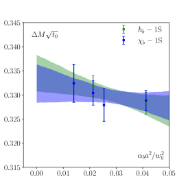
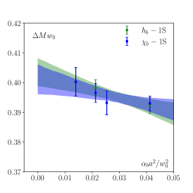
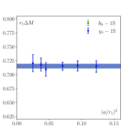
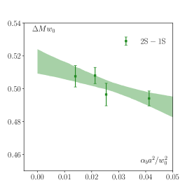
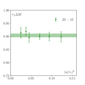
Figure 8: The continuum extrapolation of the products $\Delta M\sqrt{t_{0}}$ (left), $\Delta Mw_{0}$ (middle) and $\Delta Mr_{1}$ (right) via $\Delta M_{\mathrm{1P-1S}}$ (top) and $\Delta M_{\mathrm{2S-1S}}$ (bottom). The mass differences $\Delta M$ are taken from [48]. The bands represent the continuum extrapolation.

IV.2 Determination of the theory scales from bottomonium mass splitting

Bottomonium mass splittings are also used in the determination of the theory scales [49, 6, 50]. In this sub-section we discuss the determination of the theory scales using bottomonium splitting. We use the mass differences between different bottomonium states calculated using lattice nonrelativistic QCD (NRQCD) in [48] for $\beta=6.740,6.880,7.03,7.28,7.596$ and in [51] for $\beta=7.373$. Since the bottomonium mass differences calculated in NRQCD can be affected by missing higher order relativistic corrections as well as missing radiative corrections to the parameters of NRQCD Lagrangian, it is important to consider mass differences that minimize these effects. Considering mass differences that are not sensitive to spin-spin and spin-orbit interactions does this. We consider the following bottomonium mas differences: i) The mass difference between $h_{b}(1P)$ state the spin averaged and the spin-averaged 1S mass, defined as $M_{\mathrm{1S}}=(M_{\eta_{b}(\mathrm{1S})}+3M_{\Upsilon(\mathrm{1S})})/4$). ii) The mass difference between the spin average $\chi_{b}(1P)$ mass, defined as $M^{\chi_{b}}_{\mathrm{1P}}=(1M_{\chi_{b0}(\mathrm{1P})}+3M_{\chi_{b1}(\mathrm{1P})}+5M_{\chi_{b2}(\mathrm{1P})})/9$, and $M_{\mathrm{1S}}$ iii) The mass difference between the spin-averaged 2S state, $M_{\mathrm{2S}}=(M_{\eta_{b}(\mathrm{2S})}+3M_{\Upsilon(\mathrm{2S})})/4$, and nd the spin-averaged 1S mass, defined as $M_{\mathrm{1S}}$. We denote these mass differences as $\Delta M$ with additional labels $h_{b}-1S$, $\chi_{b}-1S$ and $2S-1S$.

Similar to previous section, we calculate the dimensionless products $\Delta M\sqrt{t_{0}}$, $\Delta Mw_{0}$ and $r_{1}\Delta M$ present on the same ensembles, and then extrapolate them to the continuum limit. The lattice spacing of these dimensionless products and the continuum extrapolations are shown in Fig. 8. For the continuum extrapolation of $\Delta M\sqrt{t_{0}}$, $\Delta Mw_{0}$ we use an ansatz linear in $\alpha_{b}a^{2}/w_{0}^{2}$ while for $r_{1}\Delta M$ we fit it to a constant, while interestingly enough this combination has no dependence on the lattice spacings within errors.

Using the values of $\Delta M$ taken from PDG [52], we can convert the products to extract the theory scales in physical units. The obtained values of the products and the theory scales are listed in Table 7. We note that even difference between the spin average bottomomonium masses we have systematic errors due to the use of NRQCD. The estimates of these errors vary depending on the details of the lattice setup and the states considered and lie between 0.2% $\sim$ 1.2% [18, 53]. We assign a 1% systematic error to the $h_{b}-1S$, $\chi_{b}-1S$ and $2S-1S$ splitting and propagate these systematic errors to the corresponding systematic errors on the values of $\sqrt{t_{0}}$, $w_{0}$ and $r_{1}$ in physical units shown as the second error in the last three columns in Table 7. The central values of the scales $\sqrt{t_{0}}$, $w_{0}$ and $r_{1}$ are larger then the ones obtain from the meson decay constant in the previous sub-section. The values of $r_{1}$ shown in Table 7 agree with the values of $r_{1}$ obtained by MILC [54, 55, 56] and HPQCD collaborations [49, 18], but are lower than the value obtained by RBC/UKQCD collaboration $r_{1}=0.333(9)$ fm [4] and another determination from HPQCD collaboration $r_{1}=0.3209(26)$ fm [18].

	$\Delta M\sqrt{t_{0}}$	$\Delta Mw_{0}$	$\Delta Mr_{1}$	$\sqrt{t_{0}}$ [fm]	$w_{0}$ [fm]	$r_{1}$ [fm]
$h_{b}-\mathrm{1S}$	0.3330(53)	0.4024(63)	0.7150 (41)	0.1453(17)(15)	0.1752(21)(18)	0.3105(18)(31)
$\chi_{b}-\mathrm{1S}$	0.3325(52)	0.4018(62)	0.7155(42)	0.1441(17)(14)	0.1739(21)(17)	0.3104(18)(31)
$\mathrm{2S}-\mathrm{1S}$	0.4243(76)	0.5128(91)	0.9036(70)	0.1477(40)(15)	0.1783(49)(18)	0.3119(76)(31)

Table 7: The continuum-extrapolated values of $\Delta M\sqrt{t_{0}}$, $\Delta Mw_{0}$ and $\Delta Mr_{1}$. The physical values of the extracted theory scales $\sqrt{t_{0}}$, $w_{0}$ and $r_{1}$ are also provided.

IV.3 Final values of the theory scales

To obtain the final values of the theory scales we take the weighted average of the different results given in the last three columns of Table 7 and in Eqs. (20), (21) and (23). We combine the statistical errors on the dimensionless products and the error on the input scale in quadrature when evaluating the total error of different determination. We obtain:

$$\begin{split}r_{1}&=0.3072\ (22)\ \mathrm{fm},\\ \sqrt{t_{0}}&=0.14229\ (98)\ \mathrm{fm},\\ w_{0}&=0.17190\ (140)\ \mathrm{fm}.\\ \end{split}$$ (24)

Since the different determination of the theory scales are correlated we took the smallest error of all possible determinations as our final error estimate in the above equations. The $r_{1}$ scale is consistent with the FLAG-2024 $N_{f}=2+1$ average of $r_{1}=$0.3127 (30) fm [45], and also with the recent $N_{f}=2+1+1$ result from the TUMQCD Collaboration, which is 0.3037 (25) fm [12], within errors. The flow scale $w_{0}$ obtained in this work is consistent with the FLAG-2024 average [45] for $N_{f}=2+1$, which reports and $w_{0}$=0.17355(92) fm as well as with the $N_{f}=2+1+1$ FLAG-2024 average [45], $w_{0}=0.17256(103)$ fm. It also agrees with the most recent BMW result [57], $w_{0}=$0.17245(22)(46)[51] fm. Our result for the gradient flow scale $\sqrt{t_{0}}$ is lower that the $N_{f}=2+1$ FLAG 2024 average [45] $\sqrt{t_{0}}$=0.14474(57) fm, but in agreement with $N_{f}=2+1+1$ FLAG 2024 average [45], $\sqrt{t_{0}}=0.14292(104)$ fm. This does not seem to be accidental, since we argued in Sec. III.2 that the gradient flow scales in $N_{f}=2+1$ and $N_{f}=2+1+1$ are expected to be the same within errors. We also note that in the recent paper the ALPHA collaboration quotes a value $\sqrt{t_{0}}=0.1439(19)$ fm [58], which is consistent with out results. A comparison of the scales determined in this work and from the literature can be found in Appendix B.

V Determination of $\Lambda_{\overline{\mathrm{MS}}}$

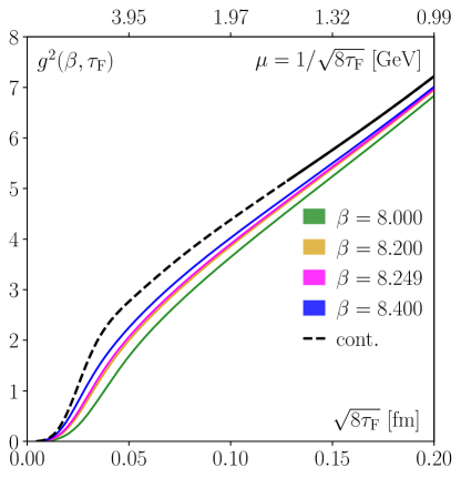
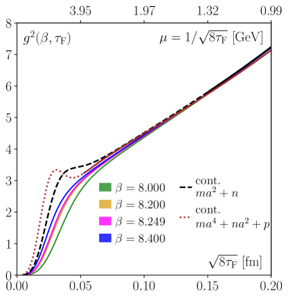
Figure 9: The strong coupling in the gradient flow scheme measured at finite lattice spacings (colored curves) and the continuum extrapolation of it (black curves). Left: Using clover-form discretization for the field strength tensor in the construction of the action density. Right: Using improved discretization for the field strength tensor. The dashed and dotted line types indicate that at this flow time the $\chi^{2}/$d.o.f of the continuum extrapolation is larger than 1.5. In the left panel we use an Ansatz linear in $a^{2}$ for the continuum extrapolation, while in the right panel we consider another Ansatz including a term quartic in $a$, which can describe the data in a much wider flow time range. The physical unit fm on $x$-axis is obtained via the $w_{0}$ scale given in Eq. (24). In these figures, the error bars are too small so we do not show them.

In this section we will determine the nonperturbative scale of strong coupling in the $\overline{\mathrm{MS}}$ scheme, $\Lambda_{\overline{\mathrm{MS}}}^{N_{f}=3}$, in 2+1 flavor QCD. The action density calculated with gradient flow can be used to define the gauge coupling in the gradient flow scheme (see e.g. [59, 60])

$$g_{\mathrm{flow}}^{2}=\frac{128\pi^{2}}{3(N_{c}^{2}-1)}\langle\tau_{\mathrm{F}}^{2}E\rangle,$$ (25)

where $N_{c}=3$ for SU(3). This definition follows the same logic as the definition of the strong coupling constant from the static quark anti-quark potential or the corresponding force, see e.g. Ref. [28]. The gradient flow coupling is defined at some energy scale, $\mu_{\mathrm{flow}}$ that is proportional to $1/\sqrt{\tau_{\mathrm{F}}}$. For sufficiently small flow time, the strong coupling in the gradient flow scheme can be related to the same in the conventionally used $\overline{\mathrm{MS}}$ scheme, $\alpha_{\overline{\mathrm{MS}}}$. This relation has been obtained by Harlander and Neumann [27] up to next-to-next-to-leading order (NNLO) in $\alpha_{\overline{\mathrm{MS}}}$, and reads

$$\begin{split}\alpha_{\mathrm{flow}}&=\alpha_{\overline{\mathrm{MS}}}\left(1+k_{1}\alpha_{\overline{\mathrm{MS}}}+k_{2}\alpha_{\overline{\mathrm{MS}}}^{2}\right)\quad\mbox{for}\;\mu_{\overline{\text{MS}}}^{2}=\mu_{\mathrm{flow}}^{2}\\ k_{1}&=1.098+0.008N_{f}\\ k_{2}&=-0.982-0.070N_{f}+0.002N_{f}^{2},\end{split}$$ (26)

where $\alpha_{\mathrm{flow}}(\mu_{\mathrm{flow}})=g_{\mathrm{flow}}^{2}/(4\pi)$. Normally $\mu_{\mathrm{flow}}=1/\sqrt{8\tau_{\mathrm{F}}}$ is used. In our case $N_{f}=3$.

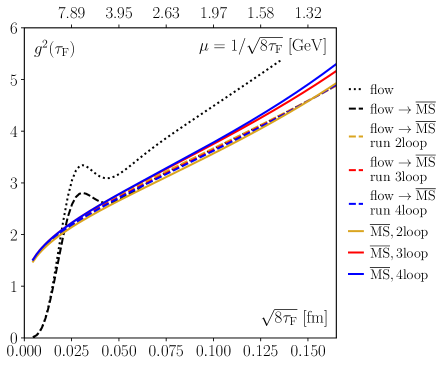
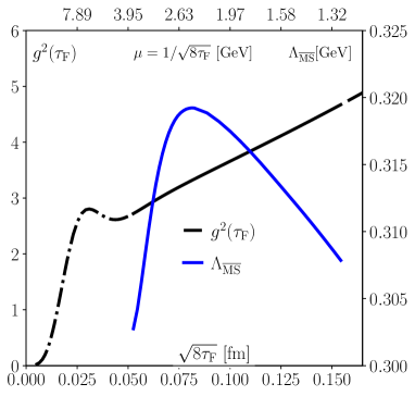
Figure 10: Left: Comparisons of $g_{\mathrm{flow}}^{2}$ (dotted black) and $g_{\mathrm{\overline{MS}}}^{2}$ obtained from different methods. The dashed black lines shows $g_{\mathrm{\overline{MS}}}^{2}$ obtained by converting $g_{\mathrm{flow}}^{2}$ through Eq. (26), the colored dashed lines are obtained via different orders of perturbative running of the flow scheme-converted $g_{\mathrm{\overline{MS}}}^{2}$ at the reference scale 1.276 GeV, and the colored solid lines corresponds to purely perturbative calculations $g^{2}_{{}_{\overline{\mathrm{MS}}}}$ using $\Lambda_{\overline{\mathrm{MS}}}=338$ MeV and $N_{f}=3$ (see text for more details). Right: The black line is same as the black dashed line in the left panel. The blue line shows the resultant $\Lambda_{\overline{\mathrm{MS}}}$ determined by a conversion between the gradient flow scheme and the $\overline{\mathrm{MS}}$ scheme within the selected ${\tau_{\mathrm{F}}}=1/(8\mu^{2})$ window indicated by solid black line and by demanding that the purely perturbative 4-loop calculations of $g^{2}_{{}_{\overline{\mathrm{MS}}}}$ with $N_{f}=3$ matches with the black line within the selected ${\tau_{\mathrm{F}}}=1/(8\mu^{2})$ window indicated by solid black line.

The lattice determination of the strong coupling using gradient flow has been explored in quenched QCD [61, 62] using small volumes and a series of lattice calculations that connect calculations in the small volumes to the physical world. Here we explore the calculation of the strong coupling using gradient flow in relatively large volumes, where the lattice spacing can be directly determined as discussed in the previous sections. First, we calculated the gradient flow coupling defined in Eq. (25) at nonzero lattice spacing. Since we need to minimize lattice artifacts when calculating the gradient flow coupling we only consider the highest four beta values, $\beta=8.0,~8.2,~8.249$ and 8.4. The gradient flow coupling calculated at these $\beta$ values using the action density with the clover discretization and the improved discretization of the field strength tensor are shown in the left and right panels of Fig. 9, respectively. The $x$-axis in fm is determined using the physical value of $w_{0}$ obtained in Eq. (24).

As the next step we need to extrapolate the results on the gradient flow coupling obtained at non-zero lattice spacings to the continuum limit. This is done using an Ansatz linear in $a^{2}$ for both discretization. For the improved discretization, we add another Ansatz containing a quartic term in $a$ to account for higher order discretization effects. We find that with this term, our data can be better described, i.e., we can obtain good fits in a wider flow time range. In Fig. 9 the fits with $\chi^{2}$/d.o.f. smaller than 1.5 are indicated by using solid black or brown lines. We observe that using the improved discretization brings the colorful curves at finite lattice spacings closer to each other than using the clover discretization. This demonstrates that the lattice cutoff effects are better controlled when using the improved discretization. Therefore, we will not use the results from the clover operator in what follows. In the right panel, two fit Ans$\ddot{\mathrm{a}}$tze give consistent results in the flow time range of interest. However, the second Ansatz is more capable of describing the higher-order discretization error. Thus, we decide to keep the results only from this Ansatz from this point onward.

Having continuum results on the gradient flow coupling we can perform the conversion to the $\overline{\text{MS}}$ scheme. In Fig. 10 (left) we show the conversion of $g^{2}$ from gradient flow scheme to $\overline{\text{MS}}$ scheme. In the left panel, the black dotted curve denotes the continuum-extrapolated results in the gradient flow scheme. The black dashed curve denotes the $\overline{\text{MS}}$ results converted from the gradient flow scheme by solving the cubic equation Eq. (26). Such conversion can be valid only within a proper flow time/energy scale window. In this region, on the one hand the lattice effects must be well controlled. This is guaranteed by choosing flow times at which $\chi^{2}$/d.o.f. is smaller than 1.5. On the other hand the perturbative effects must also be under control in this region. This can be guaranteed by only considering the energy scales that are higher (equivalently, flow time smaller) than a reference point, which we choose to be 1.278 GeV (corresponding to $\sqrt{8\tau_{\mathrm{F}}}\leq$ 0.1543 fm). Within this window, $\Lambda_{\overline{\mathrm{MS}}}$ can be determined from the converted $g^{2}_{\overline{\text{MS}}}$ at different orders. The difference of the conversion at different flow times will be quoted as one of the systematic uncertainties. In the figure, we show the running of the flow scheme-converted $g^{2}_{\overline{\text{MS}}}$ starting from the reference point to smaller flow times at different orders up to 4 loop (which is quantitatively indistinguishable from the 5 loop order) using the function crd.AlphasExact from the runDec package [63, 64] as colored dashed curves. For comparisons, we also show the purely perturbative $g^{2}_{\overline{\text{MS}}}$ calculated using runDec function crd.AlphasLam with $N_{f}=3$ and the FLAG-2024 average $\Lambda_{\overline{\mathrm{MS}}}=338$ MeV [45] as colored solid curves. Since the perturbative expansion at the 4th or 5th loop orders are indistinguishable, we do not consider 5-loop running coupling. We clearly see a significant difference between $g^{2}_{\overline{\mathrm{MS}}}$ obtained with $\Lambda_{\overline{\mathrm{MS}}}=338$ MeV and that from our flow scheme-converted one. This suggests that $\Lambda_{\overline{\mathrm{MS}}}$ determined through this approach yields a different value.

To obtain our flow scheme-converted $g^{2}_{\overline{\mathrm{MS}}}$ through the running of the strong coupling and starting from its vanishing value at an asymptotically-large energy scale, one must choose a different value of $\Lambda_{\overline{\mathrm{MS}}}$. We determine this new value of $\Lambda_{\overline{\mathrm{MS}}}$ by matching the $g^{2}_{\overline{\mathrm{MS}}}$ obtained from runDec with $N_{f}=3$ and 4-loop running to our flow scheme-converted $g^{2}_{\overline{\mathrm{MS}}}$. The results are shown in Fig. 10 (right) for each flow time ${\tau_{\mathrm{F}}}=1/(8\mu^{2})$ within the valid conversion window (indicated by solid black curve).

Since the matching relation given in Eq. (26) that maps the gradient flow coupling for some flow time to $\alpha_{\overline{\mathrm{MS}}}$ and thus also to $\Lambda_{\overline{\mathrm{MS}}}$ is not exact, the values of the $\Lambda$ parameters obtained via Eq. (26) for different $\tau_{F}$ need not to be the same. The variation of $\Lambda_{\overline{\mathrm{MS}}}$ with $\tau_{\mathrm{F}}$ indicates the importance of missing higher order corrections in Eq. (26). We see from Fig. 10 (right) that $\Lambda_{\overline{\mathrm{MS}}}^{N_{f}=3}\in[302.8,319.2]$ for the $\tau_{\mathrm{F}}$ range where we expect the perturbative correction to be reliable. We will retain only the central value of the obtained range, 311.0 MeV, and disregard the systematic uncertainty stemming from scale variation. This is because, in the subsequent analysis, we will systematically evaluate all conceivable uncertainties in this calculation, including those related to missing higher-order perturbative corrections, which inherently subsume the uncertainty addressed here. We consider three sources: i) Statistical uncertainty: This is calculated using bootstrap resampling. ii) Cut-off effects: We exclude the coarsest lattice at $\beta=8.000$ in the continuum extrapolation and take the difference from using the complete lattices as the systematic uncertainty. iii) Higher order perturbative terms in the conversion equation Eq. (26): To probe these effects we add a 3 loop term $k_{3}\alpha_{\overline{\text{MS}}}^{3}$ in Eq. (26), where $k_{3}=2k_{2}$ or $k_{3}=-2k_{2}$. The difference from not having such a term will be quoted as another systematic uncertainty. All three error analyses are conducted at $\tau_{\mathrm{F}}=0.0812$ fm, which corresponds to the maximum of the solved $\Lambda_{\overline{\mathrm{MS}}}^{N_{f}=3}$ (the peak location of the blue curve in the right panel of Fig.10). Collecting all the pieces we obtain

$$\Lambda_{\overline{\mathrm{MS}}}^{N_{f}=3}=311.0_{-0.7}^{+0.7}{}_{-4.8}^{+4.8}{}_{-11.7}^{+34.0}~{\rm MeV}.$$ (27)

Our central value for the $\Lambda$ parameter is lower than the FLAG average [45] for $N_{f}=3$ QCD $\Lambda_{\overline{\mathrm{MS}}}^{N_{f}=3}=338(10)$ MeV based on Refs. [65, 31, 66, 67, 30, 29, 68, 69, 70, 71]. However, it is still compatible with it within the estimated uncertainties. Very recently the ALPHA collaboration reported $\Lambda_{\overline{\mathrm{MS}}}=343.9(8.4)$ [58], which agrees with the above result within errors. Using the $\Lambda_{\overline{\mathrm{MS}}}^{N_{f}=3}$ obtained above, we compute $\alpha_{\overline{\mathrm{MS}}}^{(5)}(M_{Z})$ at the $Z$-boson mass by employing the decoupling relation between the strong coupling and the quark masses. This involves incrementally increasing the number of active quark flavors, starting from 3. The calculation is performed using the runDec function crd.DecAsUpMS with the following parameters: the $\overline{\mathrm{MS}}$ charm quark mass at its own scale $m_{\mathrm{charm}}$=1.275 GeV, the $\overline{\mathrm{MS}}$ bottom quark mass at its own scale $m_{\mathrm{bottom}}$=4.203 GeV, the $Z$-boson mass $M_{Z}$=91.1876 GeV, and 5-loop accuracy. The result of this computation is $\alpha_{\overline{\mathrm{MS}}}^{(5)}(M_{Z})=0.1162_{-0.0009}^{+0.0023}$, consistent with the FLAG-2024 average of 0.1183(7) [45] within the quoted errors.

VI Conclusions

In this work, we determine the gradient flow scales $\sqrt{t_{0}}$ and $w_{0}$ using Zeuthen flow with both clover and improved discretized action density in 2+1 flavor lattice QCD on HISQ ensembles at large $\beta$ values. Our results, $\sqrt{t_{0}}=0.14229(98)$ fm and $w_{0}=0.17190(140)$ fm, are consistent with the FLAG-2024 averages [45]. Using these flow scales, we calculate the potential scale $r_{1}$, which agrees within 1$\sigma$ with our results extracted from kaon and $\eta_{s}$ decay constants and within 2$\sigma$ with those from bottomonium mass splittings. Combining these determinations we obtain $r_{1}=0.3072(22)$ fm, consistent with FLAG-2024 averages [45] within 2$\sigma$. We also provide polynomial expressions for scale setting at large $\beta$, enabling reliable lattice spacing determinations for new ensembles. In addition, we determine the $\Lambda_{\overline{\mathrm{MS}}}$ parameter using gradient flow via the NNLO perturbative matching of $\alpha_{s}$ between the gradient flow and $\overline{\mathrm{MS}}$ schemes. Our final estimate is $\Lambda_{\overline{\mathrm{MS}}}=311.0_{-0.7}^{+0.7}{}_{-4.8}^{+4.8}{}_{-11.7}^{+34.0}$ MeV, leading to $\alpha_{\overline{\mathrm{MS}}}^{(5)}(M_{Z})=0.1162_{-0.0009}^{+0.0023}$. While this approach provides a reasonable determination of $\Lambda_{\overline{\mathrm{MS}}}$, further improvements in accuracy would benefit from higher-order refinements in the perturbative matching, which we leave for future work.

Appendix

Appendix A Error analysis in the calculation of flow scales

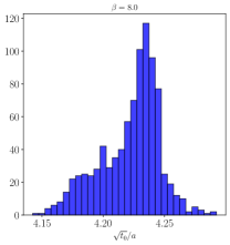
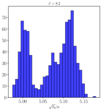
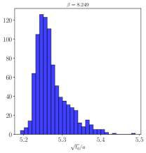
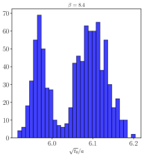
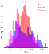
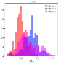
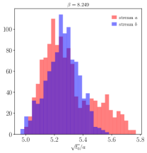
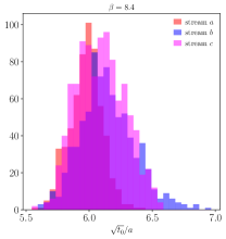
Figure 11: Top: the distribution histogram of the bootstrap samples for $\sqrt{t_{0}}/a$ using the clover discretization from the $8.000\leq\beta\leq 8.400$ lattices. Bottom: same as above but from each configuration, separated by stream.

Looking at Table 2, we noticed that among all the flow scales, $\sqrt{t_{2}}/a$ has generally the smallest statistical errors. This is because $\sqrt{t_{2}}/a$ appears at the smallest flow time, where the action density and its derivative are statistically the most precise. Besides, we also noticed that given similar statistics, the $\beta=8.249$ lattice and $\beta=8.400$ lattice have substantially different error sizes in most cases. To identify the reason, we plot the distribution histogram of the bootstrap samples of $\sqrt{t_{0}}/a$ for the clover discretization for these two lattices in Fig. 11. We note that the bootstrap samples are drawn from the binned configurations with bin-size equal twice the integrated autocorrelation time. There are 900 bootstrap samples generated in both cases. We can see that for $\beta=8.400$, there is an unusual double-peaked structure, which manifests evident systematic uncertainty. To take it into account we use the median and 68-percentile confidence interval to estimate the expectation value and the error. In this case the error band for $\beta=8.400$ will be broader than the width of any one of the two peaks.

We note that for the other lattices, only $\beta=8.200$ shows similar double-peaked structure. The $\beta=8.000$ lattice does not exhibit a double-peaked structure but an extra plateau can be identified. This hints that there are different distributions for different streams, which can be further confirmed in the bottom panel. We note that the stream ($a$, $b$, $c$) of the lattice $\beta=8.000$, 8.200, 8.400 corresponds to a single value of topological charge (2,1,0), (2,0,0), (2,0,0). There is no distinction made for the $\beta=8.249$ lattice. Fig. 11 indicates that streams of the same $Q$ tend to follow the same distribution and different $Q$ sectors give different distributions. We find that the action density seems to be sensitive to the topological charge.

Appendix B Comparison of scales from different sources

In Fig. 12 we compare the scales $r_{1}$, $\sqrt{t_{0}}$ and $w_{0}$ determined in this work and from the literature that have been included in FLAG 2024 [45].

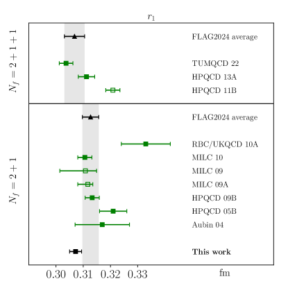
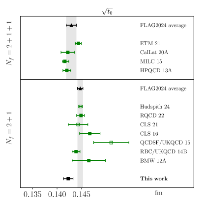
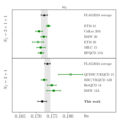
Figure 12: A comparison of scales determined in this work and from the literature that have been included in FLAG 2024 [45]. Top: $r_{1}$. Bottom left: $\sqrt{t_{0}}$. Bottom right: $w_{0}$.

References

- Blum et al. [2016] T. Blum et al. (RBC, UKQCD), Phys. Rev. D 93, 074505 (2016), arXiv:1411.7017 [hep-lat] .
- Miller et al. [2021] N. Miller et al., Phys. Rev. D 103, 054511 (2021), arXiv:2011.12166 [hep-lat] .
- Borsányi et al. [2012] S. Borsányi, S. Dürr, Z. Fodor, C. Hoelbling, S. D. Katz, S. Krieg, T. Kurth, L. Lellouch, T. Lippert, and C. McNeile (BMW), JHEP 09, 010 (2012), arXiv:1203.4469 [hep-lat] .
- Aoki et al. [2011] Y. Aoki et al. (RBC, UKQCD), Phys. Rev. D 83, 074508 (2011), arXiv:1011.0892 [hep-lat] .
- Aoki et al. [2009a] S. Aoki et al. (PACS-CS), Phys. Rev. D 79, 034503 (2009a), arXiv:0807.1661 [hep-lat] .
- Davies et al. [2010] C. T. H. Davies, E. Follana, I. D. Kendall, G. P. Lepage, and C. McNeile (HPQCD), Phys. Rev. D 81, 034506 (2010), arXiv:0910.1229 [hep-lat] .
- Sommer [1994] R. Sommer, Nucl. Phys. B 411, 839 (1994), arXiv:hep-lat/9310022 .
- Bernard et al. [2000] C. W. Bernard, T. Burch, K. Orginos, D. Toussaint, T. A. DeGrand, C. E. DeTar, S. A. Gottlieb, U. M. Heller, J. E. Hetrick, and B. Sugar, Phys. Rev. D 62, 034503 (2000), arXiv:hep-lat/0002028 .
- Francis et al. [2015] A. Francis, O. Kaczmarek, M. Laine, T. Neuhaus, and H. Ohno, Phys. Rev. D 91, 096002 (2015), arXiv:1503.05652 [hep-lat] .
- Bazavov et al. [2014] A. Bazavov et al. (HotQCD), Phys. Rev. D 90, 094503 (2014), arXiv:1407.6387 [hep-lat] .
- Bazavov et al. [2012] A. Bazavov et al., Phys. Rev. D 85, 054503 (2012), arXiv:1111.1710 [hep-lat] .
- Brambilla et al. [2023a] N. Brambilla, R. L. Delgado, A. S. Kronfeld, V. Leino, P. Petreczky, S. Steinbeißer, A. Vairo, and J. H. Weber (TUMQCD), Phys. Rev. D 107, 074503 (2023a), arXiv:2206.03156 [hep-lat] .
- Bazavov et al. [2013] A. Bazavov et al. (MILC), Phys. Rev. D 87, 054505 (2013), arXiv:1212.4768 [hep-lat] .
- Bazavov et al. [2016] A. Bazavov et al. (MILC), Phys. Rev. D 93, 094510 (2016), arXiv:1503.02769 [hep-lat] .
- Alexandrou et al. [2021] C. Alexandrou et al. (Extended Twisted Mass), Phys. Rev. D 104, 074520 (2021), arXiv:2104.06747 [hep-lat] .
- Borsanyi et al. [2021] S. Borsanyi et al., Nature 593, 51 (2021), arXiv:2002.12347 [hep-lat] .
- Bruno et al. [2017a] M. Bruno, T. Korzec, and S. Schaefer, Phys. Rev. D 95, 074504 (2017a), arXiv:1608.08900 [hep-lat] .
- Dowdall et al. [2013] R. J. Dowdall, C. T. H. Davies, G. P. Lepage, and C. McNeile, Phys. Rev. D 88, 074504 (2013), arXiv:1303.1670 [hep-lat] .
- Bornyakov et al. [2015] V. G. Bornyakov et al., (2015), arXiv:1508.05916 [hep-lat] .
- Narayanan and Neuberger [2006] R. Narayanan and H. Neuberger, JHEP 03, 064 (2006), arXiv:hep-th/0601210 .
- Luscher [2010] M. Luscher, Commun. Math. Phys. 293, 899 (2010), arXiv:0907.5491 [hep-lat] .
- Luscher and Weisz [2011] M. Luscher and P. Weisz, JHEP 02, 051 (2011), arXiv:1101.0963 [hep-th] .
- Bazavov et al. [2018a] A. Bazavov, P. Petreczky, and J. H. Weber, Phys. Rev. D 97, 014510 (2018a), arXiv:1710.05024 [hep-lat] .
- Altenkort et al. [2023a] L. Altenkort, O. Kaczmarek, R. Larsen, S. Mukherjee, P. Petreczky, H.-T. Shu, and S. Stendebach (HotQCD), Phys. Rev. Lett. 130, 231902 (2023a), arXiv:2302.08501 [hep-lat] .
- Luscher and Weisz [1985a] M. Luscher and P. Weisz, Commun. Math. Phys. 98, 433 (1985a), [Erratum: Commun.Math.Phys. 98, 433 (1985)].
- Luscher and Weisz [1985b] M. Luscher and P. Weisz, Phys. Lett. B 158, 250 (1985b).
- Harlander and Neumann [2016] R. V. Harlander and T. Neumann, JHEP 06, 161 (2016), arXiv:1606.03756 [hep-ph] .
- Necco and Sommer [2001] S. Necco and R. Sommer, Phys. Lett. B 523, 135 (2001), arXiv:hep-ph/0109093 .
- Bazavov et al. [2019] A. Bazavov, N. Brambilla, X. Garcia i Tormo, P. Petreczky, J. Soto, A. Vairo, and J. H. Weber (TUMQCD), Phys. Rev. D 100, 114511 (2019), arXiv:1907.11747 [hep-lat] .
- Ayala et al. [2020] C. Ayala, X. Lobregat, and A. Pineda, JHEP 09, 016 (2020), arXiv:2005.12301 [hep-ph] .
- Chakraborty et al. [2015] B. Chakraborty, C. T. H. Davies, B. Galloway, P. Knecht, J. Koponen, G. C. Donald, R. J. Dowdall, G. P. Lepage, and C. McNeile, Phys. Rev. D 91, 054508 (2015), arXiv:1408.4169 [hep-lat] .
- Ramos and Sint [2016] A. Ramos and S. Sint, Eur. Phys. J. C 76, 15 (2016), arXiv:1508.05552 [hep-lat] .
- Lüscher [2010] M. Lüscher, JHEP 08, 071 (2010), [Erratum: JHEP 03, 092 (2014)], arXiv:1006.4518 [hep-lat] .
- Altenkort et al. [2021a] L. Altenkort, A. M. Eller, O. Kaczmarek, L. Mazur, G. D. Moore, and H.-T. Shu, Phys. Rev. D 103, 014511 (2021a), arXiv:2009.13553 [hep-lat] .
- Altenkort et al. [2021b] L. Altenkort, A. M. Eller, O. Kaczmarek, L. Mazur, G. D. Moore, and H.-T. Shu, Phys. Rev. D 103, 114513 (2021b), arXiv:2012.08279 [hep-lat] .
- Brambilla et al. [2023b] N. Brambilla, V. Leino, J. Mayer-Steudte, and P. Petreczky (TUMQCD), Phys. Rev. D 107, 054508 (2023b), arXiv:2206.02861 [hep-lat] .
- Altenkort et al. [2023b] L. Altenkort, A. M. Eller, A. Francis, O. Kaczmarek, L. Mazur, G. D. Moore, and H.-T. Shu, Phys. Rev. D 108, 014503 (2023b), arXiv:2211.08230 [hep-lat] .
- Borsanyi et al. [2024] S. Borsanyi, Z. Fodor, J. N. Guenther, S. D. Katz, P. Parotto, A. Pasztor, D. Pesznyak, K. K. Szabo, and C. H. Wong, Phys. Rev. D 110, L011501 (2024), arXiv:2312.07528 [hep-lat] .
- Gattringer and Lang [2010] C. Gattringer and C. B. Lang, Quantum chromodynamics on the lattice, Vol. 788 (Springer, Berlin, 2010).
- Bilson-Thompson et al. [2003] S. O. Bilson-Thompson, D. B. Leinweber, and A. G. Williams, Annals Phys. 304, 1 (2003), arXiv:hep-lat/0203008 .
- Allton [1997] C. R. Allton, Nucl. Phys. B Proc. Suppl. 53, 867 (1997), arXiv:hep-lat/9610014 .
- Follana et al. [2007] E. Follana, Q. Mason, C. Davies, K. Hornbostel, G. P. Lepage, J. Shigemitsu, H. Trottier, and K. Wong (HPQCD, UKQCD), Phys. Rev. D 75, 054502 (2007), arXiv:hep-lat/0610092 .
- Brown [2018] N. J. Brown, Lattice Scales from Gradient Flow and Chiral Analysis on the MILC Collaboration’s HISQ Ensembles, Ph.D. thesis, Washington U., St. Louis, Washington U., St. Louis (2018).
- Aoki et al. [2022] Y. Aoki et al. (Flavour Lattice Averaging Group (FLAG)), Eur. Phys. J. C 82, 869 (2022), arXiv:2111.09849 [hep-lat] .
- Aoki et al. [2024] Y. Aoki et al. (Flavour Lattice Averaging Group (FLAG)), (2024), arXiv:2411.04268 [hep-lat] .
- Bazavov et al. [2010a] A. Bazavov et al. (MILC), PoS LATTICE2010, 074 (2010a), arXiv:1012.0868 [hep-lat] .
- Bazavov et al. [2018b] A. Bazavov et al., Phys. Rev. D 98, 074512 (2018b), arXiv:1712.09262 [hep-lat] .
- Larsen et al. [2020] R. Larsen, S. Meinel, S. Mukherjee, and P. Petreczky, Phys. Lett. B 800, 135119 (2020), arXiv:1910.07374 [hep-lat] .
- Gray et al. [2005] A. Gray, I. Allison, C. T. H. Davies, E. Dalgic, G. P. Lepage, J. Shigemitsu, and M. Wingate, Phys. Rev. D 72, 094507 (2005), arXiv:hep-lat/0507013 .
- Dowdall et al. [2012] R. J. Dowdall et al. (HPQCD), Phys. Rev. D 85, 054509 (2012), arXiv:1110.6887 [hep-lat] .
- Ding et al. [2025] H. T. Ding, W. P. Huang, R. Larsen, S. Meinel, S. Mukherjee, P. Petreczky, and Z. Tang, (2025), arXiv:2501.11257 [hep-lat] .
- Tanabashi et al. [2018] M. Tanabashi et al. (Particle Data Group), Phys. Rev. D 98, 030001 (2018).
- Meinel [2010] S. Meinel, Phys. Rev. D 82, 114502 (2010), arXiv:1007.3966 [hep-lat] .
- Aubin et al. [2004] C. Aubin, C. Bernard, C. DeTar, J. Osborn, S. Gottlieb, E. B. Gregory, D. Toussaint, U. M. Heller, J. E. Hetrick, and R. Sugar, Phys. Rev. D 70, 094505 (2004), arXiv:hep-lat/0402030 .
- Bazavov et al. [2009] A. Bazavov et al. (MILC), PoS CD09, 007 (2009), arXiv:0910.2966 [hep-ph] .
- Bazavov et al. [2010b] A. Bazavov et al. (MILC), Rev. Mod. Phys. 82, 1349 (2010b), arXiv:0903.3598 [hep-lat] .
- Boccaletti et al. [2024] A. Boccaletti et al., (2024), arXiv:2407.10913 [hep-lat] .
- Brida et al. [2025] M. D. Brida, R. Höllwieser, F. Knechtli, T. Korzec, A. Ramos, S. Sint, and R. Sommer, (2025), arXiv:2501.06633 [hep-ph] .
- Fodor et al. [2012] Z. Fodor, K. Holland, J. Kuti, D. Nogradi, and C. H. Wong, JHEP 11, 007 (2012), arXiv:1208.1051 [hep-lat] .
- Hasenfratz and Witzel [2020] A. Hasenfratz and O. Witzel, Phys. Rev. D 101, 034514 (2020), arXiv:1910.06408 [hep-lat] .
- Hasenfratz et al. [2023] A. Hasenfratz, C. T. Peterson, J. van Sickle, and O. Witzel, Phys. Rev. D 108, 014502 (2023), arXiv:2303.00704 [hep-lat] .
- Wong et al. [2023] C. H. Wong, S. Borsanyi, Z. Fodor, K. Holland, and J. Kuti, PoS LATTICE2022, 043 (2023), arXiv:2301.06611 [hep-lat] .
- Herren and Steinhauser [2018] F. Herren and M. Steinhauser, Comput. Phys. Commun. 224, 333 (2018), arXiv:1703.03751 [hep-ph] .
- Chetyrkin et al. [2000] K. G. Chetyrkin, J. H. Kuhn, and M. Steinhauser, Comput. Phys. Commun. 133, 43 (2000), arXiv:hep-ph/0004189 .
- McNeile et al. [2010] C. McNeile, C. T. H. Davies, E. Follana, K. Hornbostel, and G. P. Lepage, Phys. Rev. D 82, 034512 (2010), arXiv:1004.4285 [hep-lat] .
- Dalla Brida et al. [2022] M. Dalla Brida, R. Höllwieser, F. Knechtli, T. Korzec, A. Nada, A. Ramos, S. Sint, and R. Sommer (ALPHA), Eur. Phys. J. C 82, 1092 (2022), arXiv:2209.14204 [hep-lat] .
- Petreczky and Weber [2022] P. Petreczky and J. H. Weber, Eur. Phys. J. C 82, 64 (2022), arXiv:2012.06193 [hep-lat] .
- Cali et al. [2020] S. Cali, K. Cichy, P. Korcyl, and J. Simeth, Phys. Rev. Lett. 125, 242002 (2020), arXiv:2003.05781 [hep-lat] .
- Bruno et al. [2017b] M. Bruno, M. Dalla Brida, P. Fritzsch, T. Korzec, A. Ramos, S. Schaefer, H. Simma, S. Sint, and R. Sommer (ALPHA), Phys. Rev. Lett. 119, 102001 (2017b), arXiv:1706.03821 [hep-lat] .
- Aoki et al. [2009b] S. Aoki et al. (PACS-CS), JHEP 10, 053 (2009b), arXiv:0906.3906 [hep-lat] .
- Maltman et al. [2008] K. Maltman, D. Leinweber, P. Moran, and A. Sternbeck, Phys. Rev. D 78, 114504 (2008), arXiv:0807.2020 [hep-lat] .
- Mazur [2021] L. Mazur, Topological Aspects in Lattice QCD, Ph.D. thesis, Bielefeld U. (2021).
- Bollweg et al. [2022] D. Bollweg, L. Altenkort, D. A. Clarke, O. Kaczmarek, L. Mazur, C. Schmidt, P. Scior, and H.-T. Shu, PoS LATTICE2021, 196 (2022), arXiv:2111.10354 [hep-lat] .
- Mazur et al. [2024] L. Mazur et al. (HotQCD), Comput. Phys. Commun. 300, 109164 (2024), arXiv:2306.01098 [hep-lat] .