Provably Efficient RLHF Pipeline:
A Unified View from Contextual Bandits

Abstract

Reinforcement Learning from Human Feedback (RLHF) is a widely used approach for aligning Large Language Models (LLMs) with human preferences. While recent advancements have provided valuable insights into various stages and settings of RLHF, a comprehensive theoretical understanding of the entire RLHF pipeline remains lacking. Towards this end, we propose a unified framework for the RLHF pipeline from the view of contextual bandits and provide provable efficiency guarantees. In particular, we decompose the RLHF process into two distinct stages: (post-)training and deployment, exploring both passive and active data collection strategies during the training phase. By employing the Bradley-Terry preference model with a linearly parameterized reward function, we reformulate RLHF as a contextual preference bandit problem. We then develop novel algorithms for each stage, demonstrating significant improvements over existing approaches in both statistical and computational efficiency. Finally, we apply our method to train and deploy Llama-3-8B-Instruct on the Ultrafeedback-binarized dataset, and empirical results confirm the effectiveness of our approach.

1 Introduction

Table 1: Comparison between previous works and approach in terms of the statistical and computational efficiency across different stages of the RLHF pipeline. Our pipeline consists of two stages: training and deployment, where we explore both passive and active data collection strategies in the training stage. The statistical efficiency is measured using the sub-optimality gap (for the training stage) and regret (for the deployment stage), while the computational efficiency is evaluated based on time and storage complexity. Here, $d$ is the dimension of the feature space, $T$ is the number of samples, $\kappa$ is the non-linearity coefficient which can be exponentially large, $\mathbb{E}_{x\sim\rho}\left(\phi(x,\pi^{*}(x))-v\right)$ is the concentratability vector, $V_{T}$ and $\mathcal{H}_{T}$ are two kinds of local norm that satisfies $\mathcal{H}_{T}\succeq(1/\kappa)V_{T}$.

Stage	Data	Reference	Sub-optimality Gap/Regret	Time	Storage
Training	Passive	Zhu et al. (2023)	$\widetilde{\mathcal{O}}\Big{(}\kappa\sqrt{d}\cdot\big{\lVert}\mathbb{E}_{x\sim\rho}\left(\phi(x,\pi^{*}(x))-v\right)\big{\rVert}_{V_{T}^{-1}}\Big{)}$	$\mathcal{O}(T\log T)$	$\mathcal{O}(T)$
		Ours (Theorem 1)	$\widetilde{\mathcal{O}}\Big{(}\sqrt{d}\cdot\big{\lVert}\mathbb{E}_{x\sim\rho}\left(\phi(x,\pi^{*}(x))-v\right)\big{\rVert}_{\mathcal{H}_{T}^{-1}}\Big{)}$	$\mathcal{O}(T)$	$\mathcal{O}(T)$
	Active	Das et al. (2024)	$\widetilde{\mathcal{O}}\big{(}d\sqrt{\kappa/T}\big{)}$	$\mathcal{O}(T^{2}\log T)$	$\mathcal{O}(T)$
		Ours (Theorem 2)	$\widetilde{\mathcal{O}}\big{(}d\sqrt{\kappa/T}\big{)}$	$\mathcal{O}(T)$	$\mathcal{O}(1)$
Deployment	Online	Saha (2021)	$\widetilde{\mathcal{O}}\big{(}d\kappa\sqrt{T}\big{)}$	$\mathcal{O}(T^{2}\log T)$	$\mathcal{O}(T)$
		Ours (Theorem 3)	$\widetilde{\mathcal{O}}\big{(}d\sqrt{\kappa T}\big{)}$	$\mathcal{O}(T)$	$\mathcal{O}(1)$

Reinforcement Learning from Human Feedback is a key technique for training large language models using human feedback (Ouyang et al., 2022; Bai et al., 2022). The RLHF process involves collecting data, each consisting of a prompt, a pair of responses, and a human preference label indicating the preferred response. Then, a reward model is trained to predict human preferences, and the LLM is fine-tuned based on the reward model by RL algorithms, such as PPO (Schulman et al., 2017).

Given the notable success of RLHF, recent efforts have been devoted to developing a deeper theoretical understanding of this approach. Zhu et al. (2023) investigated the standard offline setting, where the learner is provided with a fixed dataset and aims to learn a policy that maximizes the expected reward. In this setting, since the learner has no control over the data collection process, the quality of the dataset becomes crucial to the performance of the learned policy and the resulting policy often performs poorly when faced with out-of-distribution data (Burns et al., 2024). In practice, the Claude (Bai et al., 2022) and LLaMA-2 (Touvron et al., 2023) projects have demonstrated that iterative RLHF can significantly enhance model performance. Motivated by these practical advancements, Xiong et al. (2024) investigated the iterative setting, where the learner randomly selects prompts from the candidate set, generates response pairs by sampling from the current policy, and then queries for feedback to update the policy accordingly. They showed that RLHF benefits from this iterative data collection process. While uniform prompt sampling as a simple approach has been proven effective, Das et al. (2024) demonstrated that it can lead to inefficient sampling and the sub-optimality gap may fail to decrease as the number of samples increases. To this end, they studied the active setting where the learner is allowed to select both prompts and responses, query for human feedback, and update the policy accordingly.

Though these works have provided valuable insights into various stages and settings of RLHF, a comprehensive theoretical understanding of the entire RLHF pipeline remains lacking. Towards this end, in this work, we propose a unified framework for the RLHF pipeline from the view of contextual bandits. Specifically, building on recent theoretical advancements (Zhu et al., 2023; Xiong et al., 2024), we leverage the Bradley-Terry preference model with a linearly parameterized reward function to reformulate RLHF as a contextual bandit problem (Abe and Long, 1999). We then decompose the RLHF process into two distinct stages: (post-)training and deployment. In the training stage, the learner’s goal is to develop a high-performing model with minimal sample queries and computational resources, where we explore both passive and active data collection strategies. In the deployment stage, the trained model is used to select good responses to user inputs while concurrently gathering informative feedback from the user for further refinement.

Building on this unified view, we revisit the existing theoretical advancements in RLHF and observe that they primarily focus on specific stages and settings of the overall pipeline. Consequently, an understanding of the entire pipeline remains lacking. Furthermore, while they have proposed various algorithms with theoretical guarantees for different stages of RLHF, the high statistical and computational complexity of their methods presents a significant challenge for practical applications. Thus, a natural question arises:

Can we develop provably efficient algorithms with improved statistical and computational efficiency for the RLHF pipeline?

In this work, we answer this question affirmatively by proposing novel algorithms for each stage of the RLHF pipeline, improving both statistical and computational efficiency over existing methods. Specifically, our contributions are summarized as follows:

• We propose a unified framework for the RLHF pipeline from the perspective of contextual bandits. We decompose the RLHF process into two stages: (post-)training and deployment, and explore both passive and active data collection strategies during training. This perspective allows us to view several prior works as focusing on specific components of the pipeline.

• We propose algorithms that are computationally and statistically more efficient than existing methods for each stage of the RLHF pipeline. Specifically, we employ online mirror descent with a tailored local norm to replace the standard maximum likelihood estimation. Additionally, we design distinct query criteria for different stages. Table 1 summarizes the comparison between previous works and ours about statistical and computational efficiency.

• We train and deploy Llama-3-8B-Instruct on the Ultrafeedback-binarized dataset using our method, testing both passive and active data collection strategies in the training stage. The empirical results validate our theoretical findings and confirm the effectiveness of our method.

Organization.

The remainder of this paper is organized as follows. We review related work in Section 2 and introduce the problem setup in Section 3. Our pipeline is presented in Sections 4 and 5, focusing on the training and deployment stages, respectively. We present experiments in Section 6 and conclude in Section 7. All proofs and experiment details are deferred to the appendix.

Notations.

For a vector $x\in\mathbb{R}^{d}$ and a positive semi-definite matrix $A\in\mathbb{R}^{d\times d}$, we define $\lVert x\rVert_{A}=\sqrt{x^{\top}Ax}$. We use the notation $\mathcal{O}(\cdot)$ to highlight various dependencies depending on the context. For the statistical efficiency, $\mathcal{O}(\cdot)$ omits only constant factors. For computational efficiency, $\mathcal{O}(\cdot)$ solely emphasizes the dependence on the number of samples as this is the primary factor influencing the complexity. Additionally, we employ $\widetilde{\mathcal{O}}(\cdot)$ to hide polylogarithmic factors.

2 Related Work

In this section, we review the works most closely related to ours.

Reinforcement Learning from Human Feedback.

Learning from human preferences with deep learning models dates back to Christiano et al. (2017) and has been recently popularized by the success of large language models (Bai et al., 2022; Touvron et al., 2023; Achiam et al., 2023). Existing results generally fall into two categories: reward-based and reward-free. Reward-based methods typically consist of two steps: reward modeling and reward maximization (Ouyang et al., 2022). Given preference data, the reward model is trained to predict preference labels, and the LLM is fine-tuned based on the reward model using RL algorithms such as PPO (Schulman et al., 2017). In contrast, reward-free methods directly optimize the LLM using human preference feedback, without relying on explicit reward modeling (Rafailov et al., 2023; Azar et al., 2024). Among these works, Direct Preference Optimization (DPO) (Rafailov et al., 2023) is one of the most popular reward-free methods, which treats generative models directly as reward models and optimizes them using human preference feedback. In this work, we focus on the reward-based RLHF methods.

Given the empirical success of RLHF, recent efforts have been devoted to developing a deeper theoretical understanding of this approach. Zhu et al. (2023) investigated the standard offline setting, where the learner is provided with a fixed dataset and aims to learn a policy that maximizes the expected reward. Xiong et al. (2024) investigated the iterative setting, where the learner randomly selects prompts from the candidate set, generates response pairs by sampling from the current policy, and then queries for feedback to update the policy accordingly. Das et al. (2024) studied the active setting where the learner is allowed to select both prompts and responses, query for feedback, and update the policy accordingly. Liu et al. (2024) focused on the dual active setting where the learner is allowed to select conversations and teachers simultaneously for feedback. Essentially, these works focus on specific stages and settings within the RLHF pipeline, while we offer a unified view on the entire process. Furthermore, we propose algorithms that are both computationally and statistically more efficient than existing methods for each stage of the RLHF pipeline.

Contextual Dueling Bandits and RL.

Dueling bandits is a variant of the multi-armed bandit problem that incorporates pairwise comparison feedback (Yue et al., 2012). Contextual dueling bandits further extend this framework by integrating context information (Dudík et al., 2015). In this setting, Saha (2021) studied the $K$-arm contextual dueling bandit problem and proposed an algorithm with a near-optimal regret guarantee. Saha et al. (2023) extended the contextual dueling bandit problem to the reinforcement learning setting, presenting an algorithm with a sublinear regret bound. Sekhari et al. (2024) further studied the contextual dueling bandit problem with active learning, where the learner is allowed to query for feedback adaptively and the goal is to minimize the regret while minimizing the number of queries simultaneously. However, these works primarily focus on the online setting, where the context is provided in an arbitrary and online manner and goal is to minimize cumulative regret. In this work, we consider the entire RLHF pipeline, including both training and deployment stages, and explore both passive and active data collection strategies in the training stage.

Active Learning.

Active learning is a well-established field that aims to reduce the labeling cost by selecting the most informative samples for annotation (Settles, 2009). The first line of work focuses on the pool-based setting (Seung et al., 1992; Freund et al., 1997; Huang et al., 2010). In this setting, the learner strategically selects a batch of the most informative data at each step and queries labels only for this selected batch. The learner then uses this labeled batch to update the model. Once the model is enhanced, the learner selects another batch of data and queries labels for it, continuing the iterative training process. The other line of work focuses on the online active setting (Cesa-Bianchi et al., 2004, 2006). In this setting, the learner sequentially observes data points and decides whether to query labels for them. Ji et al. (2024) explored the online active RLHF setting where prompts are provided in an arbitrary and online manner, with the goal of minimizing cumulative regret while minimizing the number of queries simultaneously. In this work, we leverage the pool-based active learning strategy in the training stage of the RLHF pipeline, where the learner is allowed to select the dataset actively.

3 Problem Setup

In this section, we introduce the problem setup for RLHF.

Following recent advancements in RLHF (Zhu et al., 2023; Xiong et al., 2024), we formulate RLHF as a contextual bandit problem. Specifically, we have a set of contexts $\mathcal{X}$ and a set of possible actions $\mathcal{A}$ per context. To learn with human preference feedback, the learner selects a tuple $(x,a,a^{\prime})$ to present to the human, where $x\in\mathcal{X}$ is the context, $a,a^{\prime}\in\mathcal{A}$ are the actions. The human then provides a binary preference feedback $y\in\{0,1\}$, where $y=1$ indicates the human prefers action $a$ over action $a^{\prime}$, and $y=0$ otherwise. We study the commonly used Bradley-Terry (BT) model in preference learning (Bradley and Terry, 1952), which assumes that the human’s preference is generated by a logistic function of the difference in the rewards of the two actions.

Definition 1 (Bradley-Terry Model).

Given a context $x\in\mathcal{X}$ and two actions $a,a^{\prime}\in\mathcal{A}$, the probability of the human preferring action $a$ over action $a^{\prime}$ is given by

$$\mathbb{P}\left[y=1\mid x,a,a^{\prime}\right]=\frac{\exp\left(r(x,a)\right)}{\exp\left(r(x,a)\right)+\exp\left(r\left(x,a^{\prime}\right)\right)},$$

where $r$ is a latent reward function.

We consider the linear reward model which is widely used in the RLHF literature (Zhu et al., 2023; Ji et al., 2024; Das et al., 2024).

Assumption 1.

It holds that $r(x,a)=\phi(x,a)^{\top}\theta^{*}$ where $\phi(x,a):\mathcal{X}\times\mathcal{A}\to\mathbb{R}^{d}$ is the known and fixed feature map, and $\theta^{*}\in\mathbb{R}^{d}$ is the unknown parameter vector. Furthermore, we assume $\lVert\phi(x,a)\rVert_{2}\leq L$ for all $x\in\mathcal{X}$ and $a\in\mathcal{A}$ and $\theta^{*}\in\Theta$ where $\Theta=\{\theta\in\mathbb{R}^{d}\mid\langle\bm{1},\theta\rangle=0,\|\theta\|_{2}\leq B\}$.

Remark 1.

The feature mapping $\phi$ can be constructed by removing the last layer of a pre-trained large language model, and $\theta^{*}$ corresponds to the weights of the last layer.

Based on the linear model, we can rewrite the probability as

$$\mathbb{P}\left[y=1\mid x,a,a^{\prime}\right]=\sigma\left(\phi(x,a)^{\top}\theta^{*}-\phi(x,a^{\prime})^{\top}\theta^{*}\right),$$ (1)

where $\sigma(w)=\frac{1}{1+\exp(-w)}$ is the sigmoid function. Next, we introduce a key quantity that captures learning complexity under the BT model.

Definition 2.

The non-linearity coefficient $\kappa$ is defined as

$$\kappa=\max_{x\in\mathcal{X},a,a^{\prime}\in\mathcal{A}}\max_{\theta\in\Theta}\frac{1}{\dot{\sigma}\left(\phi(x,a)^{\top}\theta-\phi(x,a^{\prime})^{\top}\theta\right)},$$ (2)

where $\dot{\sigma}(w)=\sigma(w)(1-\sigma(w))$ is the derivative function.

Remark 2.

Through direct calculation, we obtain $\kappa\leq 2+\exp(2BL)+\exp(-2BL)$. Thus, $\kappa$ may be exceedingly large with an exponential dependence on the magnitude of features and parameters, as justified in Appendix G.2.

The RLHF pipeline can generally be divided into two distinct stages: the (post-)training stage and the deployment stage, each with different objectives. In the training stage, the learner aims to develop a high-performing model with minimal samples and computational resources. In the deployment stage, the trained model is used to generate good responses to user inputs, while simultaneously gathering informative feedback for further refinement. We provide a detailed discussion of both stages in the following sections.

4 Training Stage

In the training stage, the learner aims to acquire a high-performing model with minimal number of samples and computational resources. To effectively evaluate the model’s performance, we define the following performance measure.

Performance Measure.

For any policy $\pi$, we define the sub-optimality gap compared to the optimal policy as follows:

$$\operatorname*{\mathsf{SubOpt}}(\pi)=\mathbb{E}_{x\sim\rho}\left[r\left(x,\pi^{*}(x)\right)-r(x,\pi(x)\right],$$ (3)

where $\rho$ is the context distribution, $\pi^{*}=\arg\max_{a}r(x,a)$ is the optimal policy under the true reward $r$. The goal of the learner is to minimize the performance gap $\operatorname*{\mathsf{SubOpt}}(\pi)$.

In the training stage, two data collection strategies are commonly used: passive and active. In passive setting, the learner is given a fixed set of samples. Conversely, in active setting, the learner can actively select queries for human feedback. We discuss both strategies below.

4.1 Passive Data Collection

In the passive data collection setting, we are given a fixed dataset $\left\{\left(x_{t},a_{t},a_{t}^{\prime},y_{t}\right)\right\}_{t=1}^{T}$ where $x_{t}\in\mathcal{X}$ is the context, $a_{t},a_{t}^{\prime}\in\mathcal{A}$ are the actions, and $y_{t}\in\{0,1\}$ is the feedback. Since the parameter $\theta^{*}$ is unknown, we need to estimate it from the available data. The most common method for this estimation is maximum likelihood estimation (MLE). First, let $z=\phi(x,a)-\phi(x,a^{\prime})$ be the feature difference, then we define the negative log-likelihood $\ell_{t}(\theta)$ for sample $t$ as

$$\ell_{t}(\theta)=-y_{t}\log(\sigma(z_{t}^{\top}\theta))-\left(1-y_{t}\right)\log(1-\sigma(z_{t}^{\top}\theta)).$$ (4)

The MLE estimator $\widehat{\theta}_{T+1}$ is then defined as

$$\widehat{\theta}_{T+1}=\operatorname*{arg\,min}_{\theta\in\mathbb{R}^{d}}\mathcal{L}_{T+1}(\theta)\triangleq\sum_{t=1}^{T}\ell_{t}(\theta).$$ (5)

Several works (Zhu et al., 2023; Ji et al., 2024) have analyzed the statistical properties of MLE and showed that for any $\delta\in(0,1)$, with probability at least $1-\delta$, the MLE estimator $\widehat{\theta}_{T+1}$ converges to the true parameter $\theta^{*}$ by

$$\lVert\widehat{\theta}_{T+1}-\theta^{*}\rVert_{V_{T+1}}\leq\widehat{\beta}\triangleq\widetilde{\mathcal{O}}\big{(}\kappa\sqrt{d}\big{)},$$ (6)

where $V_{t}\triangleq\sum_{i=1}^{t-1}z_{i}z_{i}^{\top}+\lambda I$ is the feature covariance matrix, $\lambda$ is the regularization parameter.

For computational complexity, the MLE estimator does not have a closed-form solution, requiring iterative optimization techniques, such as gradient descent, to obtain an $\varepsilon$-accurate solution. As discussed in Faury et al. (2022), optimizing the MLE typically requires $\mathcal{O}(\log(1/\varepsilon))$ iterations to reach the desired accuracy. Since the loss function is defined over all data samples, each iteration involves $\mathcal{O}(T)$ gradient computations. Given that $\varepsilon$ is typically set to $1/T$ to prevent it from dominating the overall estimation error, the total computational complexity is $\mathcal{O}(T\log T)$.

Although the MLE estimator is a commonly used approach, we propose a novel algorithm that enhances both computational efficiency and sample efficiency compared to MLE, drawing inspiration from recent advancements in logistic bandits (Faury et al., 2022; Zhang and Sugiyama, 2023) and multinomial logit MDPs (Li et al., 2024). First, we define the gradient $g_{t}(\theta)$ and Hessian $H_{t}(\theta)$ of the loss function $\ell_{t}(\theta)$ as

$$g_{t}(\theta)=\left(\sigma\left(z_{t}^{\top}\theta\right)-y_{t}\right)z_{t},~~H_{t}(\theta)=\dot{\sigma}\left(z_{t}^{\top}\theta\right)z_{t}z_{t}^{\top}.$$ (7)

Implicit OMD.

To improve the computational efficiency, Faury et al. (2022) observed that the cumulative past log-loss is strongly convex and can therefore be well approximated by a quadratic function. Building on this observation, they proposed the following update rule:

$$\bar{\theta}_{t+1}=\operatorname*{arg\,min}_{\theta\in\Theta}\Big{\{}\ell_{t}(\theta)+\frac{1}{2\eta}\left\|\theta-\bar{\theta}_{t}\right\|_{\bar{\mathcal{H}}_{t}}^{2}\Big{\}},$$ (8)

where $\bar{\mathcal{H}}_{t}=\sum_{i=1}^{t-1}H_{i}\left(\bar{\theta}_{i+1}\right)+\lambda I$ is the local norm, and $\eta$ is the step size. The optimization problem can be decomposed in two terms. The first term is the instantaneous log-loss $\ell_{t}(\theta)$, which accounts for the information of the current sample. The second consists of a quadratic proxy for the past losses constructed through the sequence $\{\bar{\theta}_{i}\}_{i\leq t}$. A key component is the design of the local norm $\bar{\mathcal{H}}_{t}$, which approximates the Hessian matrix by $H_{i}\left(\bar{\theta}_{i+1}\right)$ at a lookahead point $\bar{\theta}_{i+1}$. Such a Hessian matrix effectively captures local information and is crucial for ensuring statistical efficiency.

Although this formulation may appear computationally more efficient than MLE due to its one-pass data processing, the optimization problem in Eq. (8) still lacks a closed-form solution. Consequently, it still requires $\mathcal{O}(\log(1/\varepsilon))$ iterations per sample to achieve an $\varepsilon$-accurate solution, leading to the same $\mathcal{O}(T\log T)$ computational complexity as MLE.

Standard OMD.

To enhance computational efficiency, we revisit the formulation in Eq. (8) and observe that it essentially corresponds to the implicit OMD framework (Kivinen and Warmuth, 1997). Consequently, a natural alternative is to replace this formulation with the standard OMD framework, which permits a closed-form solution and thus eliminates the need for iterative optimization. However, the standard OMD minimizes a first-order approximation of the loss function, which sacrifices several key properties compared to its implicit counterpart, as demonstrated by Campolongo and Orabona (2020). Specifically, the standard OMD formulation updates using $\partial\ell_{t}(\theta_{t})$, whereas the implicit OMD updates the algorithm approximately with the subsequent sub-gradient, $\partial\ell_{t}(\theta_{t+1})$. This distinction results in a notable gap in the convergence rates of the two methods. To this end, we propose to approximate the current loss $\ell_{t}(\theta)$ using a second-order Taylor expansion, drawing inspiration from Zhang and Sugiyama (2023). We define the second-order approximation of the original loss function $\ell_{t}(\theta)$ at the current estimator $\widetilde{\theta}_{t}$ as $\widetilde{\ell}_{t}(\theta)=\ell_{t}(\widetilde{\theta}_{t})+g_{t}(\widetilde{\theta}_{t})^{\top}(\theta-\widetilde{\theta}_{t})+\frac{1}{2}\lVert\theta-\widetilde{\theta}_{t}\rVert_{H_{t}(\widetilde{\theta}_{t})}^{2}$. Then, we replace the current loss $\ell_{t}(\theta)$ in Eq. (8) with the approximation $\widetilde{\ell}_{t}(\theta)$, leading to the following update rule:

$$\widetilde{\theta}_{t+1}=\operatorname*{arg\,min}_{\theta\in\Theta}\Big{\{}\big{\langle}g_{t}(\widetilde{\theta}_{t}),\theta\big{\rangle}+\frac{1}{2\eta}\big{\|}\theta-\widetilde{\theta}_{t}\big{\|}_{\widetilde{\mathcal{H}}_{t}}^{2}\Big{\}},$$ (9)

where $\eta$ is the step size and $\widetilde{\mathcal{H}}_{t}=\mathcal{H}_{t}+\eta H_{t}(\widetilde{\theta}_{t})$ is the local norm with $\mathcal{H}_{t}\triangleq\mathcal{H}_{t}(\widetilde{\theta}_{i+1})=\sum_{i=1}^{t-1}H_{i}(\widetilde{\theta}_{i+1})+\lambda I$.

The optimization problem in Eq. (9) can be solved with a projected gradient step with the following equivalent formulation:

$$\widetilde{\theta}_{t+1}^{\prime}=\widetilde{\theta}_{t}-\eta\widetilde{\mathcal{H}}_{t}^{-1}g_{t}(\widetilde{\theta}_{t}),\quad\widetilde{\theta}_{t+1}=\operatorname*{arg\,min}_{\theta\in\Theta}\lVert\theta-\widetilde{\theta}_{t+1}^{\prime}\rVert_{\widetilde{\mathcal{H}}_{t}}^{2}.$$

Thus, the estimator $\widetilde{\theta}_{t+1}$ can be computed in an $\mathcal{O}(1)$ time complexity, leading to a total time complexity of $\mathcal{O}(T)$ for the entire procedure. This represents a significant improvement over the $\mathcal{O}(T\log T)$ complexity of the MLE estimator in Eq. (5), particularly considering that the number of samples $T$ is typically large in the training of LLMs. Furthermore, since the estimator processes the samples in a one-pass manner, it mitigates the memory burden associated with computing the gradient of the full dataset at each iteration. This makes it more suitable for large-scale applications, where memory and time efficiency are crucial.

It is important to note that the update rule in Eq. (9) represents a special case of online mirror descent, specifically, it can be derived from the following general form:

$$\widetilde{\theta}_{t+1}=\operatorname*{arg\,min}_{\theta\in\Theta}\Big{\{}\big{\langle}g_{t}(\widetilde{\theta}_{t}),\theta\big{\rangle}+\frac{1}{\eta}\mathcal{D}_{\psi_{t}}(\theta,\widetilde{\theta}_{t})\Big{\}},$$

where $\psi_{t}(\theta)=\frac{1}{2}\lVert\theta\rVert_{\widetilde{\mathcal{H}}_{t}}^{2}$ is the regularizer and $\mathcal{D}_{\psi_{t}}(\theta,\widetilde{\theta}_{t})=\psi_{t}(\theta)-\psi_{t}(\widetilde{\theta}_{t})-\langle\nabla\psi_{t}(\widetilde{\theta}_{t}),\theta-\widetilde{\theta}_{t}\rangle$ is the Bregman divergence. Therefore, we can analyze the estimation error using the online mirror descent framework (Orabona, 2019). Specifically, we have the following lemma.

Algorithm 1 Training Stage: Passive Data Collection

0: Dataset $\left\{\left(x_{t},a_{t},a_{t}^{\prime},y_{t}\right)\right\}_{t=1}^{T}$, regularization $\lambda>0$

1: Initialize $\widetilde{\theta}_{1}=0$, $\mathcal{H}_{1}=\lambda I_{d}$.

2: for $t=1,2,\ldots,T$ do

3:  Define $g_{t}(\theta)$ and $H_{t}(\theta)$ as in Eq. (7)

4:  Update $\widetilde{\mathcal{H}}_{t}=\mathcal{H}_{t}+\eta H_{t}(\widetilde{\theta}_{t})$

5:  Compute $\widetilde{\theta}_{t+1}$ by Eq. (9)

6:  Update $\mathcal{H}_{t+1}=\mathcal{H}_{t}+H_{t}(\widetilde{\theta}_{t+1})$

7: end for

8: Compute $\widetilde{J}_{T}(\pi)$ by Eq. (11)

8: Compute final policy $\pi_{T}=\operatorname*{arg\,max}_{\pi}\widetilde{J}_{T}(\pi)$

Lemma 1.

Let $\delta\in(0,1]$, set $\eta=(1/2)\log 2+\left(BL+1\right)$ and $\lambda=84\sqrt{2}\eta(dL^{2}+BL^{3})$, define the confidence set as

$$\mathcal{C}_{t}=\left\{\theta\in\Theta\mid\big{\|}\theta-\widetilde{\theta}_{t}\big{\|}_{\mathcal{H}_{t}}\leq\widetilde{\beta}_{t}\triangleq\mathcal{O}\big{(}\sqrt{d}(\log(t/\delta))^{2}\big{)}\right\}.$$

Then, we have $\operatorname{Pr}\left[\forall t\geqslant 1,\theta^{*}\in\mathcal{C}_{t}(\delta)\right]\geqslant 1-\delta$.

Intuitively, the confidence set shrinks as the number of samples $t$ increases, owing to the growing local norm $\mathcal{H}_{t}$. The local norm $\mathcal{H}_{t}$ captures the directions explored by the samples. The more we explore in a particular direction, the more accurate our estimation becomes along that direction.

By the definition of $\kappa$ in Definition 2, it holds that $\mathcal{H}_{t}\succeq(1/\kappa)V_{t}$, Lemma 1 implies $\forall t\in[T+1]$,

$$\lVert\widetilde{\theta}_{t}-\theta^{*}\rVert_{V_{t}}\leq\sqrt{\kappa}\lVert\widetilde{\theta}_{t}-\theta^{*}\rVert_{\mathcal{H}_{t}}\leq\widetilde{\mathcal{O}}\big{(}\sqrt{\kappa d}\big{)}.$$ (10)

Compared with the confidence set in Eq. (6), our confidence set strictly improves the estimation error by a factor of $\sqrt{\kappa}$. As highlighted in Remark 2, the non-linearity coefficient $\kappa$ may be exceedingly large during the training of LLMs, which makes our estimator statistically more efficient.

Pessimistic Policy.

Based on the estimator in Eq. (9), we adopt the “pessimism in the face of uncertainty” principle and define the pessimistic value function as

$$\widetilde{J}_{T}(\pi)=\min_{\theta\in\mathcal{C}_{T}}\mathbb{E}_{x\sim\rho}\left[(\phi(x,\pi(x))-v)^{\top}\theta\right]=(\bar{\phi}(\pi)-v)^{\top}\widetilde{\theta}_{T}-\widetilde{\beta}_{T}\lVert\bar{\phi}(\pi)-v\rVert_{\mathcal{H}_{T}^{-1}},$$ (11)

where $\bar{\phi}(\pi)=\mathbb{E}_{x\sim\rho}[\phi(x,\pi(x))]$ is the feature expectation of policy $\pi$, and $v$ is the baseline feature vector. While $v$ does not affect the induced policy, it may help reduce the sub-optimality gap (Zhu et al., 2023). The final policy is given by $\pi=\operatorname*{arg\,min}_{\pi}\widetilde{J}(\pi)$. The procedure is present in Algorithm 1. We show it enjoys the following guarantee.

Theorem 1.

Let $\delta\in(0,1]$, set the parameters as in Lemma 1, with probability at least $1-\delta$, Algorithm 1 ensures the following sub-optimality gap:

$${\operatorname*{\mathsf{SubOpt}}}(\pi_{T})\leq\widetilde{\mathcal{O}}\left(\sqrt{d}\cdot\big{\lVert}\mathbb{E}_{x\sim\rho}\left(\phi(x,\pi^{*}(x))-v\right)\big{\rVert}_{\mathcal{H}_{T}^{-1}}\right).$$

Remark 3.

The term $\big{\lVert}\mathbb{E}_{x\sim\rho}\left(\phi(x,\pi^{*}(x))-v\right)\big{\rVert}_{\mathcal{H}_{T}^{-1}}$ is referred to as the “concentratability coefficient”, a widely used concept in offline learning (Jin et al., 2021; Zhu et al., 2023). It measures the distribution shift between the optimal policy and the dataset distribution. A smaller concentratability coefficient value indicates that the dataset better covers the data distribution under the optimal policy, resulting in a smaller sub-optimality gap.

Comparison with Zhu et al. (2023).

Our result improves upon their work in both statistical and computational efficiency. First, similar to Eq. (10), Theorem 1 implies an $\widetilde{\mathcal{O}}\big{(}\sqrt{\kappa d}\cdot\big{\lVert}\mathbb{E}_{x\sim\rho}\left(\phi(x,\pi^{*}(x))-v\right)\big{\rVert}_{V_{T}^{-1}}\big{)}$ sub-optimality gap, improving upon theirs by a $\sqrt{\kappa}$ factor. Moreover, our estimator has an $\mathcal{O}(T)$ time complexity, more efficient than their $\mathcal{O}(T\log T)$ complexity.

4.2 Active Data Collection

In this part, we consider the active data collection setting, where the learner can actively select tuple $\{x_{t},a_{t},a^{\prime}_{t}\}_{t=1}^{T}$ to present to the human for feedback $\{y_{t}\}_{t=1}^{T}$.

Estimator Construction.

For each round $t\in[T]$, given $\left\{\left(x_{i},a_{i},a_{i}^{\prime},y_{i}\right)\right\}_{i=1}^{t-1}$, we define the loss function $\ell_{t}(\theta)$ as in Eq. (4), then the most standard approach is to estimate the parameter $\theta^{*}$ by MLE, which is given by $\widehat{\theta}_{t}=\operatorname*{arg\,min}_{\theta\in\mathbb{R}^{d}}\sum_{i=1}^{t-1}\ell_{i}(\theta)$. However, as noted before, the MLE estimator leads to a time complexity of $\mathcal{O}(t\log t)$ per round. Moreover, unlike the passive setting where the estimator is constructed only once, in the active setting, we need to construct the estimator in each round. This is prohibitively expensive for large-scale applications.

To improve the computational efficiency, we can leverage the OMD framework as in the passive data collection setting. Specifically, we construct the estimator $\widetilde{\theta}_{t}$ as in Eq. (9) by

$$\widetilde{\theta}_{t+1}=\operatorname*{arg\,min}_{\theta\in\Theta}\Big{\{}\big{\langle}g_{t}(\widetilde{\theta}_{t}),\theta\big{\rangle}+\frac{1}{2\eta}\big{\|}\theta-\widetilde{\theta}_{t}\big{\|}_{\widetilde{\mathcal{H}}_{t}}^{2}\Big{\}}.$$ (12)

Algorithm 2 Training Stage: Active Data Collection

0: Regularization $\lambda>0$, failure probability $\delta\in(0,1]$

1: Initialize $\widetilde{\theta}_{1}=0$, $\mathcal{H}_{1}=\lambda I_{d}$.

2: for $t=1,2,\ldots,T$ do

3:  Choose $(x_{t},a_{t},a_{t}^{\prime})$ by Eq. (13), observe feedback $y_{t}$

4:  Define $g_{t}(\theta)$ and $H_{t}(\theta)$ as in Eq. (7)

5:  Update $\widetilde{\mathcal{H}}_{t}=\mathcal{H}_{t}+\eta H_{t}(\widetilde{\theta}_{t})$

6:  Compute $\widetilde{\theta}_{t+1}$ by Eq. (12)

7:  Update $\mathcal{H}_{t+1}=\mathcal{H}_{t}+H_{t}(\widetilde{\theta}_{t+1})$

8: end for

9: Construct $\widetilde{r}_{T}(x,a)=\frac{1}{T}\sum_{t=1}^{T}\phi(x,a)^{\top}\widetilde{\theta}_{t},\forall x,a$

9: Compute policy $\pi_{T}(x)=\operatorname*{arg\,max}_{a\in\mathcal{A}}\widetilde{r}_{T}(x,a)$.

Query Selection.

Given the estimator $\widetilde{\theta}_{t}$, we choose the query with the maximum uncertainty inspired by (Das et al., 2024). Specifically, we choose the tuple by

$$(x_{t},a_{t},a_{t}^{\prime})=\operatorname*{arg\,max}_{x,a,a^{\prime}\in\mathcal{X}\times\mathcal{A}\times\mathcal{A}}\left\{\big{\lVert}\phi(x,a)-\phi(x,a^{\prime})\big{\rVert}_{\mathcal{H}_{t}^{-1}}\right\}.$$ (13)

Intuitively, $\mathcal{H}_{t}$ captures the directions explored so far, the selection criterion essentially seeks the tuple whose feature difference is poorly covered by the past observations.

Policy Output.

After $T$ rounds, we define the reward function as $\widetilde{r}_{T}(x,a)=\frac{1}{T}\sum_{t=1}^{T}\phi(x,a)^{\top}\widetilde{\theta}_{t}$ as the average of all the past estimations. Then, the final policy is given by

$$\pi_{T}(x)=\operatorname*{arg\,max}_{a\in\mathcal{A}}\widetilde{r}_{T}(x,a).$$ (14)

The detailed procedure is present in Algorithm 2. We show it enjoys the following guarantee.

Theorem 2.

Let $\delta\in(0,1]$, set the parameters as in Lemma 1, with probability at least $1-\delta$, Algorithm 2 ensures the following sub-optimality gap:

$$\operatorname*{\mathsf{SubOpt}}(\pi_{T})\leq\widetilde{\mathcal{O}}\big{(}d\sqrt{{\kappa}/{T}}\big{)}.$$

Remark 4.

In contrast to the passive data collection setting, the sub-optimality gap in Theorem 2 does not depend on the concentratability coefficient term. Instead, it decays at a rate of $T^{-1/2}$. This improvement arises because the active setting enables our algorithm to actively select queries with the maximum uncertainty, ensuring the uncertainty across all directions is effectively controlled.

Remark 5.

It is important to note that our result has a dependence on $\sqrt{\kappa}$. Though recent advances in the logistic bandits (Abeille et al., 2021; Zhang and Sugiyama, 2023) have shown that this dependence can be eliminated in the dominant term and shifted to lower-order terms, we believe this term remains necessary in our setting. This is due to the fact that the sub-optimality gap in our setting is defined as the difference between the reward $z^{\top}\theta^{*}$ while they focus the probability difference, i.e., $\sigma(z^{\top}\theta^{*})$. This difference prevents us from removing the $\sqrt{\kappa}$ term in our setting.

Comparison with Das et al. (2024).

Our algorithm attains the same sub-optimality gap as the work of Saha (2021), but with a significantly improved computational efficiency. Specifically, our algorithm has a time complexity of $\mathcal{O}(T)$ for the total $T$ round, which is more efficient than the $\mathcal{O}(T^{2}\log T)$ complexity of their MLE estimator. Moreover, our algorithm does not require storing the historical samples, resulting in only an $\mathcal{O}(1)$ storage complexity. In contrast, their MLE estimator necessitates storing all historical samples, leading to an $\mathcal{O}(T)$ storage complexity.

5 Deployment Stage

In the deployment stage, the learner uses the trained model to generate responses to user inputs and simultaneously gathering informative feedback to improve the model. This contrasts with the active data collection phase during training, which is focused solely on optimizing the final policy. In deployment, however, the learner is faced with a dual objective: selecting actions that maximize rewards to ensure a positive user experience, while also choosing actions that provide informative feedback for further model improvement.

Performance Measure.

To this end, we consider the cumulative regret compared to the optimal policy, which is defined as

$${\operatorname*{Reg}}_{T}=\sum_{t=1}^{T}\left(r\left(x_{t},\pi^{*}(x_{t})\right)-\frac{r\left(x_{t},a_{t}\right)+r\left(x_{t},a^{\prime}_{t}\right)}{2}\right),$$

where $\pi^{*}$ is the optimal policy, $a_{t}$ and $a^{\prime}_{t}$ are the actions selected by the learner at round $t$. This measure is stronger than the measure defined in Ji et al. (2024), which considers the gap between the optimal action and a single selected action. In the deployment phase, our proposed measure is more appropriate, as both actions must be sufficiently effective to ensure a positive user experience.

While our measure is more suitable for deployment, it also introduces significant challenges. To optimize the measure of Ji et al. (2024), the learner can exploit one action with high reward for exploitation while using the other action for exploration. In contrast, our setting requires both actions to be good enough. To address this, we propose a novel algorithm that balances exploration and exploitation for deployment. At a high level, our algorithm consists of two key components: estimator construction and query selection. We describe each component in detail below.

Estimator Construction.

The estimator construction is the same as the process used in the training stage. For each round $t\in[T]$, given $\left\{\left(x_{i},a_{i},a_{i}^{\prime},y_{i}\right)\right\}_{i=1}^{t-1}$, we construct the estimator $\widetilde{\theta}_{t}$ by OMD in an one-pass manner as in Eq. (9). Specifically, the estimator is updated by

$$\widetilde{\theta}_{t+1}=\operatorname*{arg\,min}_{\theta\in\Theta}\Big{\{}\big{\langle}g_{t}(\widetilde{\theta}_{t}),\theta\big{\rangle}+\frac{1}{2\eta}\big{\|}\theta-\widetilde{\theta}_{t}\big{\|}_{\widetilde{\mathcal{H}}_{t}}^{2}\Big{\}}.$$ (15)

Query Selection.

Unlike in the training stage, during deployment, the learner must balance exploration and exploitation to minimize regret. Specifically, the learner must select queries that are both informative and likely to yield high rewards. Focusing solely on high-reward queries may cause the learner to miss valuable feedback for model improvement, while prioritizing only informative queries could prevent reward maximization. To address this, we propose a novel strategy inspired by Saha (2021), which accounts for both reward maximization and uncertainty maximization.

Based on the estimator $\theta_{t}$, we first define the promising set $\mathcal{A}_{t}$ that only contains the actions with potential to be the best action. Specifically, we define the promising set as

$$\mathcal{A}_{t}=\big{\{}a\in\mathcal{A}\mid(\phi(x_{t},a)-\phi(x_{t},a^{\prime}))^{\top}\widetilde{\theta}_{t}+\widetilde{\beta}_{t}\lVert\phi(x_{t},a)-\phi(x_{t},a^{\prime})\rVert_{\mathcal{H}_{t}^{-1}}\geq 0,\forall a^{\prime}\in\mathcal{A}\big{\}}.$$ (16)

Then, we select the action pairs with the maximum uncertainty in the promising set, i.e.,

$$(a_{t},a_{t}^{\prime})=\operatorname*{arg\,max}_{(a,a^{\prime})\in\mathcal{A}_{t}\times\mathcal{A}_{t}}\left\|\phi(x_{t},a)-\phi(x_{t},a^{\prime})\right\|_{\mathcal{H}_{t}^{-1}}.$$ (17)

The overall algorithm is summarized in Algorithm 3. We show it enjoys the following regret bound.

Algorithm 3 Deployment Stage

0: Regularization $\lambda>0$, failure probability $\delta\in(0,1]$

1: Initialize $\widetilde{\theta}_{1}=0$, $\mathcal{H}_{1}=\lambda I_{d}$.

2: for $t=1,2,\ldots,T$ do

3:  Observes context $x_{t}$.

4:  Compute the promising set by Eq. (16)

5:  Choose duel actions by Eq. (17).

6:  Observe preference feedback $y_{t}$

7:  Update $\widetilde{\mathcal{H}}_{t}=\mathcal{H}_{t}+\eta H_{t}(\widetilde{\theta}_{t})$

8:  Compute $\widetilde{\theta}_{t+1}$ by Eq. (15)

9:  Update $\mathcal{H}_{t+1}=\mathcal{H}_{t}+H_{t}(\widetilde{\theta}_{t+1})$

10: end for

Theorem 3.

Let $\delta\in(0,1]$, set parameters as in Lemma 1, with probability at least $1-\delta$, Algorithm 3 enjoys the following regret guarantee:

$${\operatorname*{Reg}}_{T}\leq\widetilde{\mathcal{O}}\big{(}d\sqrt{{\kappa}{T}}\big{)}.$$

Comparison with Saha (2021).

Our result improves upon theirs in both computational and statistical efficiency. For statistical efficiency, our algorithm achieves a regret of $\widetilde{\mathcal{O}}\big{(}d\sqrt{{\kappa}{T}}\big{)}$, which is tighter by a factor of $\sqrt{\kappa}$ compared to their $\widetilde{\mathcal{O}}\big{(}d{\kappa}\sqrt{{T}}\big{)}$ result. For computational efficiency, our algorithm updates in an online manner, with $\mathcal{O}(1)$ storage and $\mathcal{O}(T)$ time complexity for the total $T$ rounds. In contrast, their algorithm requires storing all the data and solving an optimization problem each round, leading to $\mathcal{O}(T)$ storage and $\mathcal{O}(T^{2}\log T)$ time complexity. As $T$ is large or even infinite during deployment, our algorithm has a significant advantage in computational efficiency.

6 Experiment

In this section, we empirically evaluate the performance of our proposed method in terms of both effectiveness and efficiency. Specifically, we empirically validate our method with LLMs, and construct an online RLHF pipeline to evaluate different methods in both the training and deployment stage. Next, we first describe the experimental setup, and then present the empirical results.

Experimental Setup.

In our experiments, we employ the Llama-3-8B-Instruct  as the foundation model for reward model. We extract features $\phi(x,a)$ using last layer of the model, and the feature space dimension is $d=4096$. We use the Ultrafeedback-binarized dataset, a pro-processed version of the original Ultrafeedback dataset (Cui et al., 2023) for evaluation, which is a large-scale, fine-grained, diverse preference dataset, widely used as a benchmark for RLHF. It collects about 64, 000 prompts from diverse resources, including question answering, summarization, and dialogue generation. Each data consists of a context $x$, two responses $a$ and $a^{\prime}$, and a human preference label $y$.

Implementation Details.

All experiments in this section were performed using four Nvidia A800 (80 GB) GPUs with two Intel(R) Xeon(R) Gold 6430 CPUs. The learning rate is set to $1\times 10^{-3}$ for all methods. We use DeepSpeed (Rasley et al., 2020) with mixed-precision training (BF16). The maximum sequence length is set to 1024 tokens, and we use a global batch size of 32. For practical efficiency, we implement our method using Hessian-vector product (HVP) and conjugate gradient methods, which efficiently approximate the Hessian matrix without the need for computing $d^{2}$ matrix. We use the default partition of the Ultrafeedback-binarized dataset with the standard train_prefs split for training and test_prefs split for evaluation. Furthermore, we also enable flash attention for the improved training efficiency.

6.1 Training Stage

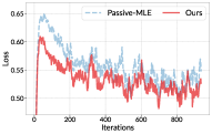
(a) training loss

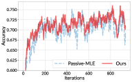
(b) training accuracy

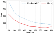
(c) evaluation loss

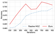
(d) evaluation accuracy

Figure 1: For the training stage with passive data collection, we compare our method with MLE (Zhu et al., 2023). We report the average accuracy and loss of the reward model during training.

In this part, we conduct experiments to evaluate the performance of our method in the training stage, including both passive and active data collection strategies.

Contenders.

In the training stage, we compare with:

• Random: A baseline that randomly selects queries.

• Passive-MLE (Zhu et al., 2023): A method that uses maximum likelihood estimation to learn the reward function and compute the pessimistic policy based on the learned reward model.

• Active-MLE (Das et al., 2024): A method using MLE to optimize the reward model and selects queries based on uncertainty, i.e., the maximum difference of two actions.

We compared our method with other methods in terms of the accuracy of the reward model, as the method for training the final policy based on the learned reward model is the same as contenders.

Passive Data Collection Results.

We first evaluate our method in the passive data collection setting. We randomly sample $T=30,000$ data points from the Ultrafeedback dataset for training. Figure 1 shows the loss and accuracy vs. the number of training samples. We observe that our method converges faster to a lower loss and achieves a higher evaluation accuracy compared to baselines. The improvement is particularly pronounced in the small-sample regime ($T<10,000$), where our method achieves a higher evaluation accuracy with the same amount of samples compared to Passive-MLE which employs conventional stochastic gradient descent (SGD) updates. This demonstrates the superior statistical efficiency of our approach, therefore achieving a better performance with fewer training samples.

Active Data Collection Results.

We then evaluate our method in the active data collection setting. In this scenario, the global batch size is set to 8, and we only allow the method to select 6, 400 samples out of the whole training datasets for training according to different selection strategies. Table 2 and Figure 2 demonstrate that our active learning strategy achieves comparable performance to passive learning while using only 21% of the labeled data. Specifically, our method achieves an average accuracy of 70.43% after 6,400 actively selected samples, which is comparable with the previous state-of-the-art method, Active-MLE, while our method is 3 times faster because we do not need to recompute all the selected data in the buffer, but we update the model in an online manner. The training loss curves in Figure 2(a) also show that our method converges faster compared to other contenders. This improved sample efficiency can be attributed to our theoretically-motivated query selection criterion that effectively identifies the most informative samples, which further validates the two key factors in our method: (1) the use of local norm $\mathcal{H}_{t}$ that better captures the uncertainty in different directions, and (2) the computationally efficient one-pass update rule that enables processing large-scale datasets.

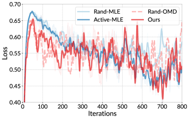
(a) training loss

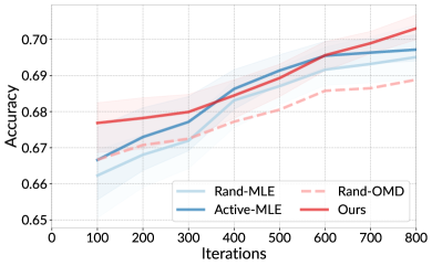
(b) evaluation accuracy

Figure 2: For the training stage with active data collection, we report (a) the training loss vs. the training iterations, and (b) the evaluation accuracy vs. the training iterations.

Method	ACC (%)	Time (s)
Rand-MLE	69.51$\pm$0.5	4876$\pm$47
Active-MLE	69.82$\pm$0.4	4982$\pm$52
Rand-OMD	68.97$\pm$0.6	1456$\pm$31
Ours	70.43$\pm$0.3	1489$\pm$36

Table 2: Comparison of different methods in terms of evaluation accuracy and training time in seconds. Results are averaged over five runs.

6.2 Deployment Stage

In this part, we evaluate our method on deployment stage.

Contenders.

In the deployment stage, we compare with:

• Random: A baseline strategy that randomly select responses from responses generated by the current policy model.

• Best-Two: A baseline strategy that selects the best two responses from responses generated by the current policy model.

• Iterative-RLHF (Dong et al., 2024): A method that takes the best and the worst responses from the current policy model to construct a new preference pair for RLHF iteratively.

Deployment Stage Analysis.

For the scenario of deployment stage, we evaluate on a pre-processed online-variant of the Ultrafeedback-binarized dataset, where we divide the dataset into 20 chunks and process them sequentially to simulate the online deployment scenario. As shown in Figure 3, our method consistently outperforms the baselines in terms of both average cumulative rewards and win rates. The average cumulative rewards in Figure 3(a) show that our method learns more effectively from interactions, achieving higher rewards over time. The win rates in Figure 3(b) demonstrate that our method makes better decisions when selecting between response pairs, outperforming both the baseline methods of Random and Best-Two, and also better than Iterative-RLHF which selects the best and worst response pairs for training. The superior performance of our method further validates the effectiveness of our theoretically grounded action selection strategy. This success stems from an efficient online update mechanism that enables rapid adaptation to new preference feedback, as well as the design of the promising set, which balances high-reward responses for immediate performance with sufficient exploration for future model improvements. These results align with our theoretical analysis in Section 5, validating the practical effectiveness of our proposed algorithm in the deployment stage.

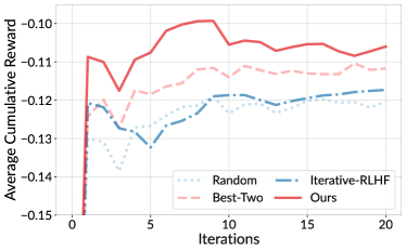
(a) average cumulative rewards

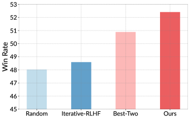
(b) win rates

Figure 3: For the deployment stage, we divide the Ultrafeedback dataset into 20 chunks, and report (a) the average cumulative rewards and the (b) win rates of different methods.

7 Conclusion and Future Work

In this work, we present a unified framework of the RLHF pipeline from the view of contextual bandits, leveraging the Bradley-Terry preference model with a linearly parameterized reward function. We decompose the RLHF process into two stages: (post-)training and deployment, exploring both passive and active data collection strategies during the training phase. We then develop novel algorithms for each stage, applying online mirror descent with a tailored local norm to replace standard maximum likelihood estimation, and designing distinct query criteria for different stages. Our theoretical analysis shows that our method improves upon existing methods in both statistical and computational efficiency. Finally, we train and deploy Llama-3-8B-Instruct on the Ultrafeedback-binarized dataset using our approach. The empirical results validate our theoretical findings and confirm the effectiveness of our proposed method.

While our work advances the theoretical understanding of RLHF, several important directions remain for future work. First, we considered the fixed feature mapping $\phi$ for the reward model, but in practice, this mapping may evolve during the training process. Thus, analyzing this dynamic feature mapping is an important future work. Second, though we focused on the Bradley-Terry model, there are other preference models for human feedback, such as the Plackett-Luce model (Luce, 1959; Plackett, 1975). Extending our results to these preference models is another promising direction.

Appendix A Useful Lemmas

Lemma 2.

For any $t\in[T]$, define the second-order approximation of the loss function $\ell_{t}(\theta)$ at the estimator $\widetilde{\theta}_{t}$ as

$$\widetilde{\ell}_{t}(\theta)=\ell_{t}(\widetilde{\theta}_{t})+\langle\nabla\ell_{t}(\widetilde{\theta}_{t}),\theta-\widetilde{\theta}_{t}\rangle+\frac{1}{2}\lVert\theta-\widetilde{\theta}_{t}\rVert_{H_{t}(\widetilde{\theta}_{t})}^{2}.$$

Then, for the following update rule

$$\widetilde{\theta}_{t+1}=\operatorname*{arg\,min}_{\theta\in\Theta}\left\{\widetilde{\ell}_{t}(\theta)+\frac{1}{2\eta}\lVert\theta-\widetilde{\theta}_{t}\rVert_{\mathcal{H}_{t}}^{2}\right\},$$

it holds that

$$\lVert\widetilde{\theta}_{t+1}-\theta^{*}\rVert_{\mathcal{H}_{t+1}}^{2}$$

$$\leq{} 2\eta\left(\sum_{i=1}^{t}\ell_{i}(\theta^{*})-\sum_{i=1}^{t}\ell_{i}(\widetilde{\theta}_{i+1})\right)+4\lambda B^{2}+12\sqrt{2}BL^{3}\eta\sum_{i=1}^{t}\lVert\widetilde{\theta}_{i+1}-\widetilde{\theta}_{i}\rVert_{2}^{2}-\sum_{i=1}^{t}\lVert\widetilde{\theta}_{i+1}-\widetilde{\theta}_{i}\rVert_{\mathcal{H}_{i}}^{2}.$$

Proof.

Based on the analysis of (implicit) OMD update (see Lemma 5), for any $i\in[T]$, we have

$$\big{\langle}\nabla\widetilde{\ell}_{i}(\widetilde{\theta}_{i+1}),\widetilde{\theta}_{i+1}-\theta^{*}\big{\rangle}\leqslant\frac{1}{2\eta}\left(\|\widetilde{\theta}_{i}-\theta^{*}\|_{\mathcal{H}_{i}}^{2}-\|\widetilde{\theta}_{i+1}-\theta^{*}\|_{\mathcal{H}_{i}}^{2}-\|\widetilde{\theta}_{i+1}-\widetilde{\theta}_{i}\|_{\mathcal{H}_{i}}^{2}\right)$$

According to Lemma 6, we have

$$\ell_{i}(\widetilde{\theta}_{i+1})-\ell_{i}\left(\theta^{*}\right)\leqslant\big{\langle}\nabla\ell_{i}(\widetilde{\theta}_{i+1}),\widetilde{\theta}_{i+1}-\theta^{*}\big{\rangle}-\frac{1}{\zeta}\big{\|}\widetilde{\theta}_{i+1}-\theta^{*}\big{\|}_{\nabla^{2}\ell_{i}(\widetilde{\theta}_{i+1})}^{2},$$

where $\zeta=\log 2+2(LB+1)$. Then, by combining the above two inequalities, we have

$$\ell_{i}(\widetilde{\theta}_{i+1})-\ell_{i}(\theta^{*}) \leqslant\langle\nabla\ell_{i}(\widetilde{\theta}_{i+1})-\nabla\widetilde{\ell}_{i}(\widetilde{\theta}_{i+1}),\widetilde{\theta}_{i+1}-\theta^{*}\rangle$$

$$\qquad+\frac{1}{\zeta}\Big{(}\|\widetilde{\theta}_{i}-\theta^{*}\|_{\mathcal{H}_{i}}^{2}-\|\widetilde{\theta}_{i+1}-\theta^{*}\|_{\mathcal{H}_{i+1}}^{2}-\|\widetilde{\theta}_{i+1}-\widetilde{\theta}_{i}\|_{\mathcal{H}_{i}}^{2}\Big{)}.$$

We can further bound the first term of the right-hand side as:

$$\big{\langle}\nabla\ell_{i}(\widetilde{\theta}_{i+1})-\nabla\widetilde{\ell}_{i}(\widetilde{\theta}_{i+1}),\widetilde{\theta}_{i+1}-\theta^{*}\big{\rangle}=\ \big{\langle}\nabla\ell_{i}(\widetilde{\theta}_{i+1})-\nabla\ell_{i}(\widetilde{\theta}_{i})-\nabla^{2}\ell_{i}(\widetilde{\theta}_{i})(\widetilde{\theta}_{i+1}-\widetilde{\theta}_{i}),\widetilde{\theta}_{i+1}-\theta^{*}\big{\rangle}$$

$$=\ \big{\langle}D^{3}\ell_{i}({\xi}_{i+1})[\widetilde{\theta}_{i+1}-\widetilde{\theta}_{i}](\widetilde{\theta}_{i+1}-\widetilde{\theta}_{i}),\widetilde{\theta}_{i+1}-\theta^{*}\big{\rangle}$$

$$\leqslant\ 3\sqrt{2}L\big{\|}\widetilde{\theta}_{i+1}-\theta^{*}\big{\|}_{2}\big{\|}\widetilde{\theta}_{i+1}-\widetilde{\theta}_{i}\big{\|}_{\nabla^{2}\ell_{i}({\xi}_{i+1})}^{2}$$

$$\leqslant\ 6\sqrt{2}BL\big{\|}\widetilde{\theta}_{i+1}-\widetilde{\theta}_{i}\big{\|}_{\nabla^{2}\ell_{i}({\xi}_{i+1})}^{2}$$

$$\leqslant\ 6\sqrt{2}BL^{3}\big{\|}\widetilde{\theta}_{i+1}-\widetilde{\theta}_{i}\big{\|}_{2}^{2},$$

where the second equality holds by the mean value theorem, the first inequality holds by the self-concordant-like property of $\ell_{i}(\cdot)$ in Lemma 3, and the last inequality holds by $\widetilde{\theta}_{i+1}$ and $\theta^{*}$ belong to $\Theta=\{\theta\in\mathbb{R}^{d},\lVert\theta\rVert_{2}\leq B\}$, and ${\nabla^{2}\ell_{i}({\xi}_{i+1})}\preceq L^{2}I_{d}$.

Then, by taking the summation over $i$ and rearranging the terms, we obtain

$$\big{\|}\widetilde{\theta}_{t+1}-\theta^{*}\big{\|}_{\mathcal{H}_{t+1}}^{2}$$

$$\leqslant\ \zeta\left(\sum_{i=1}^{t}\ell_{s}\left(\theta^{*}\right)-\sum_{i=1}^{t}\ell_{s}(\widetilde{\theta}_{i+1})\right)+\|\widetilde{\theta}_{1}-\theta^{*}\|_{\mathcal{H}_{1}}^{2}+6\sqrt{2}BL^{3}\zeta\sum_{i=1}^{t}\big{\|}\widetilde{\theta}_{i+1}-\widetilde{\theta}_{i}\big{\|}_{2}^{2}-\sum_{i=1}^{t}\big{\|}\widetilde{\theta}_{i+1}-\widetilde{\theta}_{i}\big{\|}_{\mathcal{H}_{i}}^{2}$$

$$\leqslant\ \zeta\left(\sum_{i=1}^{t}\ell_{s}\left(\theta^{*}\right)-\sum_{i=1}^{t}\ell_{s}\big{(}\widetilde{\theta}_{i+1}\big{)}\right)+4\lambda B^{2}+6\sqrt{2}BL^{3}\zeta\sum_{i=1}^{t}\big{\|}\widetilde{\theta}_{i+1}-\widetilde{\theta}_{i}\big{\|}_{2}^{2}-\sum_{i=1}^{t}\big{\|}\widetilde{\theta}_{i+1}-\widetilde{\theta}_{i}\big{\|}_{\mathcal{H}_{i}}^{2},$$

where the last inequality is by $\|\widetilde{\theta}_{1}-\theta^{*}\|_{\mathcal{H}_{1}}^{2}\leq\lambda\|\widetilde{\theta}_{1}-\theta^{*}\|_{2}^{2}\leq 4\lambda B^{2}$. Set $\zeta=2\eta$ finishes the proof. ∎

Appendix B Proof of Lemma 1

Proof.

Based on Lemma 2, we have

$$\lVert\widetilde{\theta}_{t+1}-\theta^{*}\rVert_{\mathcal{H}_{t+1}}^{2}$$

$$\leq{} 2\eta\left(\sum_{i=1}^{t}\ell_{i}(\theta^{*})-\sum_{i=1}^{t}\ell_{i}(\widetilde{\theta}_{i+1})\right)+4\lambda B^{2}+12\sqrt{2}BL^{3}\eta\sum_{i=1}^{t}\lVert\widetilde{\theta}_{i+1}-\widetilde{\theta}_{i}\rVert_{2}^{2}-\sum_{i=1}^{t}\lVert\widetilde{\theta}_{i+1}-\widetilde{\theta}_{i}\rVert_{\mathcal{H}_{i}}^{2}.$$

It remains to bound the right-hand side of the above inequality in the following. The most challenging part is to bound the term $\sum_{i=1}^{t}\ell_{i}(\theta^{*})-\sum_{i=1}^{t}\ell_{i}(\widetilde{\theta}_{i+1})$. This term might seem straightforward to control, as it can be observed that $\theta^{*}=\operatorname*{arg\,min}_{\theta\in\mathbb{R}^{d}}\bar{\ell}(\theta)\triangleq\mathbb{E}_{y_{i}}[\ell_{i}(\theta)]$, where $\ell_{i}(\theta)$ serves as an empirical observation of $\bar{\ell}(\theta)$. Consequently, the loss gap term seemingly can be bounded using appropriate concentration results. However, a caveat lies in the fact that the update of the estimator $\widetilde{\theta}_{i+1}$ depends on $\ell_{i}$, or more precisely $y_{i}$, making it difficult to directly apply such concentrations.

To address this issue, following the analysis in Zhang and Sugiyama [2023], we decompose the loss gap into two components by introducing an intermediate term. Specifically, we define the softmax function as

$$[\sigma_{i}(q)]_{1}=\frac{\exp(q)}{1+\exp(q)}\quad\text{and}\quad[\sigma_{i}(q)]_{0}=\frac{1}{1+\exp(q)},$$

where $[\cdot]_{i}$ denotes the $i$-th element of the vector. Then, the loss function $\ell_{i}(\theta)$ can be rewritten as

$$\ell(q_{t},y_{t})=-\mathds{1}_{\{y_{t}=1\}}\cdot\log\left({[\sigma(q_{t})]_{1}}\right)-\mathds{1}_{\{y_{t}=0\}}\cdot\log\left({[\sigma(q_{t})]_{0}}\right).$$

Then, we define the pseudo-inverse function of $\sigma^{-1}(p)$ with

$$[\sigma^{-1}(p)]=\log({q}/({1-q}))\quad\text{and}\quad[\sigma^{-1}(p)]_{0}=\log((1-q)/{q}).$$

Then, we decompose the regret into two terms by introducing an intermediate term.

$$\sum_{i=1}^{t}\ell_{s}\left(\theta^{*}\right)-\sum_{i=1}^{t}\ell_{s}(\widetilde{\theta}_{i+1})= \underbrace{\sum_{i=1}^{t}\ell_{s}\left(\theta^{*}\right)-\sum_{i=1}^{t}\ell_{s}(q_{i},y_{i})}_{\mathtt{term~(a)}}+\underbrace{\sum_{i=1}^{t}\ell_{s}(q_{i},y_{i})-\sum_{i=1}^{t}\ell_{s}(\widetilde{\theta}_{i+1})}_{\mathtt{term~(b)}}$$

where $q_{i}$ is an aggregating forecaster for logistic loss defined by $q_{i}=\sigma^{-1}(\mathbb{E}_{\theta\sim P_{i}}[\sigma(\theta^{\top}z_{i})])$ and $P_{i}=\mathcal{N}(\widetilde{\theta}_{i},(1+c\mathcal{H}_{i}^{-1}))$ is the Gaussian distribution with mean $\widetilde{\theta}_{i}$ and covariance $(1+c\mathcal{H}_{i}^{-1})$, where $c>0$ is a constant to be specified later. It remains to bound the terms $\mathtt{term~(a)}$ and $\mathtt{term~(b)}$, which were initially analyzed in Zhang and Sugiyama [2023] and further refined by Lee and Oh [2024]. Specifically, using Lemmas F.2 and F.3 in Lee and Oh [2024], we can bound them as follows.

For $\mathtt{term~(a)}$, let $\delta\in(0,1)$ and $\lambda\geq 1$. With probability at least $1-\delta$, for all $t\in[T]$, we have

$$\mathtt{term~(a)}\leq\left(3\log(1+2t)+2+LB\right)\left(\frac{17}{16}\lambda+2\sqrt{\lambda}\log\left(\frac{2\sqrt{1+2t}}{\delta}\right)+16\left(\log\left(\frac{2\sqrt{1+2t}}{\delta}\right)\right)^{2}\right)+2.$$

For $\mathtt{term~(b)}$, let $\lambda\geq\max\{2,72cd\}$. Then, for all $t\in[T]$, we have

$$\mathtt{term~(b)}\leq\frac{1}{2c}\sum_{i=1}^{t}\Big{\|}\widetilde{\theta}_{i+1}-\widetilde{\theta}_{i}\Big{\|}_{\mathcal{H}_{i}}^{2}+\sqrt{6}cd\log\left(1+\frac{2tB^{2}}{d\lambda}\right)$$

Combing the above two bounds, we have

$$\big{\|}\widetilde{\theta}_{t+1}-\theta^{*}\big{\|}_{\mathcal{H}_{t+1}}^{2} \leq 2\eta\left(3\log(1+2t)+2+BL\right)\left(\frac{17}{16}\lambda+2\sqrt{\lambda}\log\left(\frac{2\sqrt{1+2t}}{\delta}\right)+16\left(\log\left(\frac{2\sqrt{1+2t}}{\delta}\right)\right)^{2}\right)$$

$$\hskip-51.21495pt+4\eta+2\eta\sqrt{6}cd\log\left(1+\frac{2tL^{2}}{d\lambda}\right)+4\lambda L_{\theta}^{2}+12\sqrt{2}BL^{3}\eta\sum_{i=1}^{t}\left\|\widetilde{\theta}_{i+1}-\widetilde{\theta}_{i}\right\|_{2}^{2}+\left(\frac{\eta}{c}-1\right)\sum_{i=1}^{t}\left\|\widetilde{\theta}_{i+1}-\widetilde{\theta}_{i}\right\|_{\mathcal{H}_{i}}^{2}.$$

Setting $c=7\eta/6$ and $\lambda\geq 84\sqrt{2}BL^{3}\eta$, we have

$$12\sqrt{2}BL^{3}\eta\sum_{i=1}^{t}\left\|\widetilde{\theta}_{i+1}-\widetilde{\theta}_{i}\right\|_{2}^{2}+\left(\frac{\eta}{c}-1\right)\sum_{i=1}^{t}\left\|\widetilde{\theta}_{i+1}-\widetilde{\theta}_{i}\right\|_{\mathcal{H}_{i}}^{2}\leq\left(12\sqrt{2}BL^{3}\eta-\frac{\lambda}{7}\right)\sum_{i=1}^{t}\left\|\widetilde{\theta}_{i+1}-\widetilde{\theta}_{i}\right\|_{2}^{2}\leq 0.$$

Note that $84\sqrt{2}\left(BL^{3}+dL^{2}\right)\eta\geq\max\left\{2L^{2},72cdL^{2},84\sqrt{2}BL^{3}\eta\right\}$, so we set $\lambda\geq 84\sqrt{2}\left(BL^{3}+\right.$ $\left.dL^{2}\right)\eta$. As we have $\eta=(1/2)\log 2+\left(BL+1\right)$, we have

$$\big{\|}\widetilde{\theta}_{t+1}-\theta^{*}\big{\|}_{\mathcal{H}_{t+1}}\leq\mathcal{O}\Big{(}\sqrt{d}(\log(t/\delta))^{2}\Big{)}.$$

This finishes the proof. ∎

Appendix C Proof of Theorem 1

Proof.

Define $J(\pi)=\mathbb{E}_{x\sim\rho}[r\left(x,\pi(x)\right)]$, $J^{\prime}(\pi)=J(\pi)-\langle\theta^{*},v\rangle$, we have

$$\operatorname*{\mathsf{SubOpt}}\left(\pi_{T}\right)=\left(J^{\prime}\left(\pi^{*}\right)-\widetilde{J}\left(\pi^{*}\right)\right)+\left(\widetilde{J}\left(\pi^{*}\right)-\widetilde{J}\left(\pi_{T}\right)\right)+\left(\widetilde{J}\left(\pi_{T}\right)-J^{\prime}\left(\pi_{T}\right)\right).$$

Since $\pi_{T}$ is the optimal policy under expected value $\widetilde{J}(\pi)$, i.e., $\widetilde{J}(\pi_{T})=\max_{\pi\in\Pi}\widetilde{J}(\pi)$, we have

$$\widetilde{J}\left(\pi^{*}\right)-\widetilde{J}\left(\pi_{T}\right)\leq 0$$ (18)

For the third term, we have with probability at least $1-\delta$, it holds that

$$\widetilde{J}\left(\pi_{T}\right)-J^{\prime}\left(\pi_{T}\right)=\min_{\theta\in\mathcal{C}_{T}}\mathbb{E}_{x\sim\rho}\left[\theta^{\top}(\phi(s,\pi_{T}(s))-v)\right]-\mathbb{E}_{x\sim\rho}\left[\theta^{*\top}(\phi(s,\pi_{T}(s))-v)\right]\leq 0,$$ (19)

where the last inequality holds by $\theta^{*}\in\mathcal{C}_{T}$ with probability at least $1-\delta$.

For the first term, we have with probability at least $1-\delta$, it holds that

$$J^{\prime}\left(\pi^{*}\right)-\widetilde{J}\left(\pi^{*}\right)$$

$$=\ \mathbb{E}_{x\sim\rho}\left[(\theta^{*})^{\top}(\phi(s,\pi^{*}(s))-v)\right]-\min_{\theta\in\mathcal{C}_{T}}\mathbb{E}_{x\sim\rho}\left[\theta^{\top}(\phi(s,\pi^{*}(s))-v)\right]$$

$$=\ \sup_{\theta\in\mathcal{C}_{T}}\mathbb{E}_{x\sim\rho}\left[\left(\theta^{*}-\widetilde{\theta}_{T}+\widetilde{\theta}_{T}-\theta\right)^{\top}\left(\phi(x,\pi^{*}(x))-v\right)\right]$$

$$=\ \mathbb{E}_{x\sim\rho}\left[\left(\theta^{*}-\widetilde{\theta}_{T}\right)^{\top}\left(\phi(x,\pi^{*}(x))-v\right)\right]+\sup_{\theta\in\mathcal{C}_{T}}\mathbb{E}_{x\sim\rho}\left[\left(\widetilde{\theta}_{T}-\theta\right)^{\top}\left(\phi(x,\pi^{*}(x))-v\right)\right]$$

$$\leq\ \Big{(}\lVert\theta^{*}-\widetilde{\theta}_{T}\rVert_{\mathcal{H}_{T}}+\sup_{\theta\in\mathcal{C}_{T}}\lVert\theta-\widetilde{\theta}_{T}\rVert_{\mathcal{H}_{T}^{-1}}\Big{)}\cdot\big{\lVert}\mathbb{E}_{x\sim\rho}\left(\phi(x,\pi^{*}(x))-v\right)\big{\rVert}_{\mathcal{H}_{T}^{-1}},$$

where the first inequality holds by the Cauchy-Schwarz inequality.

Since it holds $\widetilde{\theta}_{T}\in\mathcal{C}_{T}$ with probability at least $1-\delta$ by Lemma 1, we have $\lVert\theta^{*}-\widetilde{\theta}_{T}\rVert_{\mathcal{H}_{T}}\leq\widetilde{\beta}_{T}$ and $\sup_{\theta\in\mathcal{C}_{T}}\lVert\theta-\widetilde{\theta}_{T}\rVert_{\mathcal{H}_{T}}\leq\widetilde{\beta}_{T}$. Thus, we obtain

$$J^{\prime}\left(\pi^{*}\right)-\widetilde{J}\left(\pi^{*}\right)\leq\ 2\widetilde{\beta}_{T}\cdot\big{\lVert}\mathbb{E}_{x\sim\rho}\left(\phi(x,\pi^{*}(x))-v\right)\big{\rVert}_{\mathcal{H}_{T}^{-1}}.$$ (20)

Combining Eq. (18), Eq. (19), and Eq. (20) and substituting $\widetilde{\beta}_{T}=\mathcal{O}(\sqrt{d}(\log(T/\delta))^{2})$, we have with probability at least $1-\delta$, it holds that

$$\operatorname*{\mathsf{SubOpt}}\left(\pi_{T}\right) =\left(J^{\prime}\left(\pi^{*}\right)-\widetilde{J}\left(\pi^{*}\right)\right)+\left(\widetilde{J}\left(\pi^{*}\right)-\widetilde{J}\left(\pi_{T}\right)\right)+\left(\widetilde{J}\left(\pi_{T}\right)-J^{\prime}\left(\pi_{T}\right)\right)$$

$$\leq 2\widetilde{\beta}_{T}\cdot\big{\lVert}\mathbb{E}_{x\sim\rho}\left(\phi(x,\pi^{*}(x))-v\right)\big{\rVert}_{\mathcal{H}_{T}^{-1}}$$

$$\leq\mathcal{O}\left(\sqrt{d}\left(\log\frac{T}{\delta}\right)^{2}\cdot\big{\lVert}\mathbb{E}_{x\sim\rho}\left(\phi(x,\pi^{*}(x))-v\right)\big{\rVert}_{\mathcal{H}_{T}^{-1}}\right).$$

This completes the proof. ∎

Appendix D Proof of Theorem 2

Proof.

Let the sub-optimality gap for a context $x\in\mathcal{X}$ be denoted as $\operatorname*{\mathsf{SubOpt}}(x)$. Thus, for any $\delta\in(0,1)$, with probability at least $1-\delta$, we have

$$\operatorname*{\mathsf{SubOpt}}(x) =\left(\phi\left(x,\pi^{*}(x)\right)-\phi\left(x,\pi_{T}(x)\right)\right)^{\top}\theta^{*}$$

$$\leq\left(\phi\left(x,\pi^{*}(x)\right)-\phi\left(x,\pi_{T}(x)\right)\right)^{\top}\theta^{*}+\left(\phi\left(x,\pi_{T}(x)\right)-\phi\left(x,\pi^{*}(x)\right)\right)^{\top}\left(\frac{1}{T}\sum_{t=1}^{T}\widetilde{\theta}_{t}\right)$$

$$=\left(\phi\left(x,\pi^{*}(x)\right)-\phi\left(x,\pi_{T}(x)\right)\right)^{\top}\left(\theta^{*}-\frac{1}{T}\sum_{t=1}^{T}\widetilde{\theta}_{t}\right)$$

$$=\frac{1}{T}\sum_{t=1}^{T}\left(\phi\left(x,\pi^{*}(x)\right)-\phi\left(x,\pi_{T}(x)\right)\right)^{\top}\left(\theta^{*}-\widetilde{\theta}_{t}\right)$$

$$\leq\frac{1}{T}\sum_{t=1}^{T}\left\|\phi\left(x,\pi^{*}(x)\right)-\phi\left(x,\pi_{T}(x)\right)\right\|_{\mathcal{H}_{t}^{-1}}\left\|\theta^{*}-\widetilde{\theta}_{t}\right\|_{\mathcal{H}_{t}}$$

$$\leq\frac{\widetilde{\beta}_{T}}{T}\sum_{t=1}^{T}\left\|\phi\left(x,\pi^{*}(x)\right)-\phi\left(x,\pi_{T}(x)\right)\right\|_{\mathcal{H}_{t}^{-1}},$$

where the first inequality is due to the fact that $\left(\phi\left(x,\pi_{T}(x)\right)-\phi\left(x,\pi^{*}(x)\right)\right)^{\top}\left(\frac{1}{T}\sum_{t=1}^{T}\widetilde{\theta}_{t}\right)\geq 0$ by the design of $\pi_{T}(x)$, the second is due to the Cauchy-Schwarz inequality, and the last inequality is due to $\|\theta^{*}-\widetilde{\theta}_{t}\|_{\mathcal{H}_{t}}\leq\beta_{T}$ with probability at least $1-\delta$ by Lemma 1.

By our algorithm’s choice $(x_{t},a_{t},a_{t}^{\prime})=\operatorname*{arg\,max}_{x\in\mathcal{X},a,a^{\prime}\in\mathcal{A}}\left\|\phi(x,a)-\phi\left(x,a^{\prime}\right)\right\|_{\mathcal{H}_{t}^{-1}}$, we have

$$\sum_{t=1}^{T}\left\|\phi\left(x,\pi^{*}(x)\right)-\phi\left(x,\pi_{T}(x)\right)\right\|_{\mathcal{H}_{t}^{-1}}\leq\sum_{t=1}^{T}\left\|\phi\left(x_{t},a_{t}\right)-\phi\left(x_{t},a_{t}^{\prime}\right)\right\|_{\mathcal{H}_{t}^{-1}}=\sum_{t=1}^{T}\left\|z_{t}\right\|_{\mathcal{H}_{t}^{-1}}.$$

Furthermore, by the definition of $\mathcal{H}_{t}$, we have

$$\mathcal{H}_{t}=\lambda I_{d}+\sum_{s=1}^{t-1}\dot{\sigma}\left(z_{s}^{\top}\widetilde{\theta}_{s+1}\right)z_{s}z_{s}^{\top}\geq\lambda I_{d}+\frac{1}{\kappa}\sum_{s=1}^{t-1}z_{s}z_{s}^{\top}=\frac{1}{\kappa}\left(\kappa\lambda I_{d}+\sum_{s=1}^{t-1}z_{s}z_{s}^{\top}\right)\triangleq\frac{1}{\kappa}V_{t}.$$

Thus, we have

$$\sum_{t=1}^{T}\left\|z_{t}\right\|_{\mathcal{H}_{t}^{-1}}\leq\sqrt{\kappa}\sum_{t=1}^{T}\left\|z_{t}\right\|_{V_{t}^{-1}}\leq\sqrt{\kappa}\sqrt{T\sum_{t=1}^{T}\left\|z_{t}\right\|^{2}_{V_{t}^{-1}}}\leq\sqrt{2\kappa dT\log\left(1+\frac{4TL^{2}}{\lambda\kappa d}\right)},$$

where the first inequality holds by the fact that $\mathcal{H}_{t}\succeq\frac{1}{\kappa}V_{t}$, the second inequality holds by the Cauchy-Schwarz inequality, and the last inequality holds by the elliptic potential lemma in Lemma 4. Thus, we have for any context $x\in\mathcal{X}$,

$$\operatorname*{\mathsf{SubOpt}}(x)\leq\frac{\widetilde{\beta}_{T}}{T}\sqrt{2\kappa dT\log\left(1+\frac{4TL^{2}}{\lambda\kappa d}\right)}.$$

By the definition of $\operatorname*{\mathsf{SubOpt}}(\pi_{T})$, we have with probability at least $1-\delta$,

$$\operatorname*{\mathsf{SubOpt}}\left(\pi_{T}\right)=\mathbb{E}_{x\sim\rho}\left[\operatorname*{\mathsf{SubOpt}}(x)\right]\leq\frac{\widetilde{\beta}_{T}}{T}\sqrt{2\kappa dT\log\left(1+\frac{T}{\lambda\kappa d}\right)}\leq\widetilde{\mathcal{O}}\left(d\sqrt{\frac{\kappa}{T}}\right).$$

This finishes the proof. ∎

Appendix E Proof of Theorem 3

Proof.

We first analyze the instantaneous regret at round $t$. For any $\delta\in(0,1)$, with probability at least $1-\delta$, it holds that

$$\big{(}r(x_{t},\pi^{*}(x_{t}))-r(x_{t},a_{t})\big{)}+\big{(}r(x_{t},\pi^{*}(x_{t}))-r(x_{t},a_{t}^{\prime})\big{)}$$

$$=\ \big{(}\phi(x_{t},\pi^{*}(x_{t}))-\phi(x_{t},a_{t})\big{)}^{\top}\theta^{*}+\big{(}\phi(x_{t},\pi^{*}(x_{t}))-\phi(x_{t},a_{t}^{\prime})\big{)}^{\top}\theta^{*}$$

$$=\ \big{(}\phi(x_{t},\pi^{*}(x_{t}))-\phi(x_{t},a_{t})\big{)}^{\top}\widetilde{\theta}_{t}+\big{(}\phi(x_{t},\pi^{*}(x_{t}))-\phi(x_{t},a_{t})\big{)}^{\top}(\theta^{*}-\widetilde{\theta}_{t})$$

$$+\big{(}\phi(x_{t},\pi^{*}(x_{t}))-\phi(x_{t},a_{t}^{\prime})\big{)}^{\top}\widetilde{\theta}_{t}+\big{(}\phi(x_{t},\pi^{*}(x_{t}))-\phi(x_{t},a_{t}^{\prime})\big{)}^{\top}(\theta^{*}-\widetilde{\theta}_{t})$$

$$\leq\ \widetilde{\beta}_{t}\big{\lVert}\phi(x_{t},\pi^{*}(x_{t}))-\phi(x_{t},a_{t})\big{\rVert}_{\mathcal{H}_{t}^{-1}}+\big{\lVert}\phi(x_{t},\pi^{*}(x_{t}))-\phi(x_{t},a_{t})\big{\rVert}_{\mathcal{H}_{t}^{-1}}\big{\lVert}\theta^{*}-\widetilde{\theta}_{t}\big{\rVert}_{\mathcal{H}_{t}}$$

$$+\widetilde{\beta}_{t}\big{\lVert}\phi(x_{t},\pi^{*}(x_{t}))-\phi(x_{t},a^{\prime}_{t})\big{\rVert}_{\mathcal{H}_{t}^{-1}}+\big{\lVert}\phi(x_{t},\pi^{*}(x_{t}))-\phi(x_{t},a^{\prime}_{t})\big{\rVert}_{\mathcal{H}_{t}^{-1}}\big{\lVert}\theta^{*}-\widetilde{\theta}_{t}\big{\rVert}_{\mathcal{H}_{t}}$$

$$\leq\ \widetilde{\beta}_{t}\lVert\phi(x_{t},\pi^{*}(x_{t}))-\phi(x_{t},a_{t})\rVert_{\mathcal{H}_{t}^{-1}}+\widetilde{\beta}_{t}\lVert\phi(x_{t},\pi^{*}(x_{t}))-\phi(x_{t},a_{t})\rVert_{\mathcal{H}_{t}^{-1}}$$

$$+\widetilde{\beta}_{t}\lVert\phi(x_{t},\pi^{*}(x_{t}))-\phi(x_{t},a_{t}^{\prime})\rVert_{\mathcal{H}_{t}^{-1}}+\widetilde{\beta}_{t}\lVert\phi(x_{t},\pi^{*}(x_{t}))-\phi(x_{t},a_{t}^{\prime})\rVert_{\mathcal{H}_{t}^{-1}}$$

$$\leq\ 4\widetilde{\beta}_{t}\lVert\phi(x_{t},a_{t})-\phi(x_{t},a_{t}^{\prime})\rVert_{\mathcal{H}_{t}^{-1}}.$$

Here, the first inequality holds since both $a_{t},a^{\prime}_{t}\in\mathcal{A}_{t}$ and by the definition of $\mathcal{A}_{t}$, it implies that

$$\big{(}\phi(x_{t},\pi^{*}(x_{t}))-\phi(x_{t},a_{t})\big{)}^{\top}\widetilde{\theta}_{t} \leq\widetilde{\beta}_{t}\big{\lVert}\phi(x_{t},\pi^{*}(x_{t}))-\phi(x_{t},a_{t})\big{\rVert}_{\mathcal{H}_{t}^{-1}},$$

$$\big{(}\phi(x_{t},\pi^{*}(x_{t}))-\phi(x_{t},a^{\prime}_{t})\big{)}^{\top}\widetilde{\theta}_{t} \leq\widetilde{\beta}_{t}\big{\lVert}\phi(x_{t},\pi^{*}(x_{t}))-\phi(x_{t},a_{t}^{\prime})\big{\rVert}_{\mathcal{H}_{t}^{-1}}.$$

The second inequality holds by selection strategy of $(a_{t},a_{t}^{\prime})$, it holds that

$$\lVert\phi(x_{t},\pi^{*}(x_{t}))-\phi(x_{t},a_{t})\rVert_{\mathcal{H}_{t}^{-1}} \leq\lVert\phi(x_{t},a_{t})-\phi(x_{t},a_{t}^{\prime})\rVert_{\mathcal{H}_{t}^{-1}},$$

$$\lVert\phi(x_{t},\pi^{*}(x_{t}))-\phi(x_{t},a^{\prime}_{t})\rVert_{\mathcal{H}_{t}^{-1}} \leq\lVert\phi(x_{t},a_{t})-\phi(x_{t},a_{t}^{\prime})\rVert_{\mathcal{H}_{t}^{-1}}.$$

Thus, we have

$${\operatorname*{Reg}}_{T}=\frac{1}{2}\Big{(}\big{(}r(x_{t},\pi^{*}(x_{t}))-r(x_{t},a_{t})\big{)}+\big{(}r(x_{t},\pi^{*}(x_{t}))-r(x_{t},a_{t}^{\prime})\big{)}\Big{)}\leq 2\widetilde{\beta}_{T}\sum_{t=1}^{T}\lVert\phi(x_{t},a_{t})-\phi(x_{t},a_{t}^{\prime})\rVert_{\mathcal{H}_{t}^{-1}}.$$

Furthermore, by the definition of $\mathcal{H}_{t}$, we have

$$\mathcal{H}_{t}=\lambda I_{d}+\sum_{s=1}^{t-1}\dot{\sigma}\left(z_{s}^{\top}\widetilde{\theta}_{s+1}\right)z_{s}z_{s}^{\top}\geq\lambda I_{d}+\frac{1}{\kappa}\sum_{s=1}^{t-1}z_{s}z_{s}^{\top}=\frac{1}{\kappa}\left(\kappa\lambda I_{d}+\sum_{s=1}^{t-1}z_{s}z_{s}^{\top}\right)\triangleq\frac{1}{\kappa}V_{t}$$

Thus, we obtain

$$\sum_{t=1}^{T}\left\|z_{t}\right\|_{\mathcal{H}_{t}^{-1}}\leq\sqrt{\kappa}\sum_{t=1}^{T}\left\|z_{t}\right\|_{V_{t}^{-1}}\leq\sqrt{\kappa}\sqrt{T\sum_{t=1}^{T}\left\|z_{t}\right\|^{2}_{V_{t}^{-1}}}\leq\sqrt{2\kappa dT\log\left(1+\frac{4TL^{2}}{\lambda\kappa d}\right)},$$

where the first inequality holds by the fact that $\mathcal{H}_{t}\succeq\frac{1}{\kappa}V_{t}$, the second inequality holds by the Cauchy-Schwarz inequality, and the last inequality holds by the elliptic potential lemma in Lemma 4. Thus, we have with probability at least $1-\delta$,

$${\operatorname*{Reg}}_{T}\leq 2{\widetilde{\beta}_{T}}\sqrt{2\kappa dT\log\left(1+\frac{4TL^{2}}{\lambda\kappa d}\right)}\leq\widetilde{\mathcal{O}}\left(d\sqrt{{\kappa}{T}}\right).$$

This finishes the proof. ∎

Appendix F Supporting Lemmas

Definition 3 (Tran-Dinh et al. [2015]).

A convex function $f\in\mathcal{C}^{3}\left(\mathbb{R}^{m}\right)$ is $M$-self-concordant-like function if

$$\left|\psi^{\prime\prime\prime}(s)\right|\leqslant M\|\mathbf{b}\|_{2}\psi^{\prime\prime}(s),$$

for $s\in\mathbb{R}$ and $M>0$, where $\psi(s):=f(\mathbf{a}+s\mathbf{b})$ for any $\mathbf{a},\mathbf{b}\in\mathbb{R}^{m}$.

Lemma 3 (Lee and Oh [2024, Proposition C.1]).

The loss $\ell_{t}(\theta)$ defined in Eq. (4) is $3\sqrt{2}L$-self-concordant-like for $\forall t\in[T]$.

Lemma 4 (Abbasi-Yadkori et al. [2011, Lemma 11]).

Suppose $x_{1},\ldots,x_{t}\in\mathbb{R}^{d}$ and for any $1\leq s\leq t$, $\lVert x_{s}\rVert_{2}\leq L$. Let $V_{t}=\lambda I_{d}+\sum_{s=1}^{t-1}x_{s}x_{s}^{\top}$ for $\lambda\geq 0$. Then, we have

$$\sum_{s=1}^{t}\left\|z_{s}\right\|_{V_{s}^{-1}}^{2}\leq 2d\log\left(1+\frac{tL^{2}}{\lambda d}\right).$$

Lemma 5 (Campolongo and Orabona [2020, Proposition 4.1]).

Define $\mathbf{w}_{t+1}$ as the solution of

$$\mathbf{w}_{t+1}=\operatorname*{arg\,min}_{\mathbf{w}\in\mathcal{V}}\big{\{}\eta\ell_{t}(\mathbf{w})+\mathcal{D}_{\psi}\left(\mathbf{w},\mathbf{w}_{t}\right)\big{\}},$$

where $\mathcal{V}\subseteq\mathcal{W}\subseteq\mathbb{R}^{d}$ is a non-empty convex set. Further supposing $\psi(\mathbf{w})$ is 1 -strongly convex w.r.t. a certain norm $\|\cdot\|$ in $\mathcal{W}$, then there exists a $\mathbf{g}_{t}^{\prime}\in\partial\ell_{t}\left(\mathbf{w}_{t+1}\right)$ such that

$$\left\langle\eta_{t}\mathbf{g}_{t}^{\prime},\mathbf{w}_{t+1}-\mathbf{u}\right\rangle\leq\left\langle\nabla\psi\left(\mathbf{w}_{t}\right)-\nabla\psi\left(\mathbf{w}_{t+1}\right),\mathbf{w}_{t+1}-\mathbf{u}\right\rangle$$

for any $\mathbf{u}\in\mathcal{W}$.

Lemma 6 (Zhang and Sugiyama [2023, Lemma 1]).

Let $\ell(\mathbf{z},y)=\sum_{k=0}^{K}\mathbf{1}\{y=k\}\cdot\log\left(\frac{1}{[\sigma(\mathbf{z})]_{k}}\right)$ where $\sigma(\mathbf{z})_{k}=\frac{e^{z_{k}}}{\sum_{j=0}^{K}e^{z_{j}}}$, $\mathbf{a}\in[-C,C]^{K}$, $y\in\{0\}\cup[K]$ and $\mathbf{b}\in\mathbb{R}^{K}$ where $C>0$. Then, we have

$$\ell(\mathbf{a},y)\geq\ell(\mathbf{b},y)+\nabla\ell(\mathbf{b},y)^{\top}(\mathbf{a}-\mathbf{b})+\frac{1}{\log(K+1)+2(C+1)}(\mathbf{a}-\mathbf{b})^{\top}\nabla^{2}\ell(\mathbf{b},y)(\mathbf{a}-\mathbf{b}).$$

Appendix G Details of Experiments

In this section, we provide the omitted details of the experiment details and additional results.

G.1 Implementation Details

Datasets.   We use the UltraFeedback-binarized dataset [Rafailov et al., 2023] for the experiments. This dataset is derived from the original UltraFeedback dataset, which comprises 64, 000 prompts sourced from diverse datasets including UltraChat, ShareGPT, Evol-Instruct, TruthfulQA, FalseQA, and FLAN. For each prompt, four model completions were generated using various open-source and proprietary language models, with GPT-4 providing comprehensive evaluations across multiple criteria including helpfulness, honesty, and truthfulness. The binarized version was constructed by selecting the completion with the highest overall score as the ”chosen” response and randomly selecting one of the remaining completions as the ”rejected” response, creating clear preference pairs suitable for reward modeling and direct preference optimization. This dataset structure aligns well with our experimental setup, providing a robust foundation for evaluating different preference learning approaches. The dataset’s diverse prompt sources and evaluation criteria make it particularly valuable for training and evaluating reward models in a real-world context. To further tailor the dataset to our experimental setup, we organize the dataset as follows for the training and deployment stages:

• Training stage with passive data collection: We randomly sample $T=30,000$ data points from the UltraFeedback-binarized dataset’s train_prefs split for training. Each data point consists of a prompt and two responses with a binary preference label indicating the preferred response. We use the test_prefs split for evaluation.

• Training stage with active data collection: We allow the method to actively select 6,400 samples from the train_prefs split according to different selection strategies. The global batch size is set to 8 for training. The selection is performed iteratively, where in each iteration, the method selects the most informative samples based on its selection criterion.

• Deployment stage: We use a pre-processed online variant of the UltraFeedback-binarized dataset from the test_gen split. The dataset is divided into 20 sequential chunks to simulate an online deployment scenario. For each chunk, we generate responses using the current policy (the foundation model of policy model is chosen to be meta-llama / Llama-3.2-1B), evaluate them using both the learned reward model and an oracle reward model. We choose NCSOFT/Llama-3-OffsetBias-RM-8B [Park et al., 2024] as the oracle reward model. After each chunk, we use the policy model to randomly generate 64 responses using different seeds. We then apply various strategies (Random, Best-Two, etc.) to select responses and construct new preference pairs, which are then used to update the reward model and the policy model.

Algorithm 4 Efficient Update using Hessian-Vector Product with Conjugate Gradient

0: Current parameter $\widetilde{\theta}_{t}$, gradient $g_{t}(\widetilde{\theta}_{t})$, learning rate $\eta$, max CG steps $K$, base damping $\lambda_{0}$, error tolerance $\epsilon$

1: Initialize $v_{0}=0$, $r_{0}=g_{t}(\widetilde{\theta}_{t})$, $p_{0}=r_{0}$

2: Compute damping $\lambda_{t}=\lambda_{0}\cdot\min\{1,f(t/T)\}$

3: for $k=0,1,\ldots,K-1$ do

4:  Compute HVP: $\widetilde{\mathcal{H}}_{t}p_{k}=\nabla_{\theta}(\nabla_{\theta}\mathcal{L}(\theta)^{\top}p_{k})|_{\theta=\widetilde{\theta}_{t}}+\lambda_{t}p_{k}$

5:  $\alpha_{k}=\frac{r_{k}^{\top}r_{k}}{p_{k}^{\top}\widetilde{\mathcal{H}}_{t}p_{k}}$, $v_{k+1}=v_{k}+\alpha_{k}p_{k}$, $r_{k+1}=r_{k}-\alpha_{k}\widetilde{\mathcal{H}}_{t}p_{k}$,

6:  $\beta_{k+1}=\frac{r_{k+1}^{\top}r_{k+1}}{r_{k}^{\top}r_{k}}$, $p_{k+1}=r_{k+1}+\beta_{k+1}p_{k}$

7:  if $\|r_{k+1}\|\leq\epsilon$ then

8:   break

9:  end if

10: end for

11: Update parameter: $\widetilde{\theta}_{t+1}=\widetilde{\theta}_{t}-\eta v_{K}$

11: Updated parameter $\widetilde{\theta}_{t+1}$

Practical Implementation.   To efficiently implement the OMD update in Eq. (9) without the costly computing and storing the full Hessian matrix, we utilize the Hessian-vector product (HVP) method combined with conjugate gradient descent. The key insight is that the update can be reformulated as solving a linear system. For the OMD update:

$$\widetilde{\theta}_{t+1} =\operatorname*{arg\,min}_{\theta\in\Theta}\Big{\{}\big{\langle}g_{t}(\widetilde{\theta}_{t}),\theta\big{\rangle}+\frac{1}{2\eta}\big{\|}\theta-\widetilde{\theta}_{t}\big{\|}_{\widetilde{\mathcal{H}}_{t}}^{2}\Big{\}}\approx\widetilde{\theta}_{t}-\eta\widetilde{\mathcal{H}}_{t}^{-1}g_{t}(\widetilde{\theta}_{t}),$$

where we ignore the projection operation. The key challenge is computing $\widetilde{\mathcal{H}}_{t}^{-1}g_{t}(\widetilde{\theta}_{t})$ efficiently. Instead of explicitly computing $\widetilde{\mathcal{H}}_{t}^{-1}$, we solve the linear system $\widetilde{\mathcal{H}}_{t}v=g_{t}(\widetilde{\theta}_{t})$

$$\widetilde{\mathcal{H}}_{t}v=g_{t}(\widetilde{\theta}_{t}),$$

where $v$ is the solution we seek. We use the conjugate gradient method with a damped Hessian to solve this system iteratively. The HVP operation $\widetilde{\mathcal{H}}_{t}v$ for any vector $v$ can be computed efficiently using automatic differentiation $\widetilde{\mathcal{H}}_{t}v=\nabla_{\theta}\big{(}\nabla_{\theta}\mathcal{L}(\theta)^{\top}v\big{)}\big{|}_{\theta=\widetilde{\theta}_{t}}+\lambda v$, where $\lambda$ is a damping coefficient that ensures numerical stability and $\mathcal{L}(\theta)$ is the loss function. The full algorithm is summarized in Algorithm 4. To ensure stability and convergence, we employ an adaptive damping strategy as $\lambda_{t}=\lambda_{0}\cdot\min\{1,f(t/T)\}$, where $f(\cdot)$ is a damping growth function that can be linear, logarithmic, or cosine. In practice, we set $K=3$ and $\lambda_{0}=0.8$ for all experiments.

G.2 Validating the Magnitude of $\kappa$

We validate the magnitude of $\kappa$ in Eq. (2) by computing its value during the training process. The results show that $\kappa=171.62\pm 85.49$ during our training process, which is relatively large.

G.3 Combined with Adam Optimizer

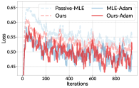
(a) training loss

(b) training accuracy

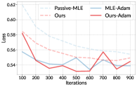
(c) evaluation loss

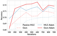
(d) evaluation accuracy

Figure 4: For the training stage with passive data collection, we compare our proposed method and MLE [Zhu et al., 2023] in with passive data collection combined with Adam. We report the average accuracy and loss of the reward model during the training process.

In previous experiments, we used SGD to update model parameters. In this section, we integrate the methods with the Adam optimizer [Kingma and Ba, 2015], i.e., adding the first and second momentum terms to the model updates. The results, shown in Figure 4, indicate that the Adam optimizer further enhances the performance of our method by leveraging the momentum term to accelerate convergence. With the momentum term, our method remains superior to the MLE-based method; however, the performance gap is reduced. We think that this is because the Adam optimizer incorporates second-order information for optimization, diminishing the advantage of our method compared to the SGD cases.

G.4 Comparison with DPO

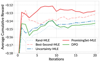
Figure 5: Comparison with DPO in the deployment stage.

We also compare with DPO (Direct Preference Optimization) [Rafailov et al., 2023] in the deployment stage, as a reward-free method, DPO optimizes the policy directly using preference feedback without explicit reward modeling. To ensure a fair comparison, we initialize the policy with 400 samples and use the same dataset settings as PPO to iteratively update the policy model using the DPO algorithm. The results are illustrated in Figure 5. While DPO outperforms the random baseline (Rand-MLE), it achieves lower cumulative rewards than the PromisingSet-based method. This result suggests that DPO’s online learning capability remains a challenge. In contrast, the reward model learned by our selection strategy effectively learned streaming data and continuously updates the policy as new data arrive, indicating that in our deployment stage, a reward model with PPO may be a more suitable choice for sequentially learning from new data.

References

- Abbasi-Yadkori et al. [2011] Yasin Abbasi-Yadkori, Dávid Pál, and Csaba Szepesvári. Improved algorithms for linear stochastic bandits. In Advances in Neural Information Processing Systems 24 (NIPS), pages 2312–2320, 2011.
- Abe and Long [1999] Naoki Abe and Philip M. Long. Associative reinforcement learning using linear probabilistic concepts. In Proceedings of the 16th International Conference on Machine Learning (ICML), pages 3–11. Morgan Kaufmann, 1999.
- Abeille et al. [2021] Marc Abeille, Louis Faury, and Clément Calauzènes. Instance-wise minimax-optimal algorithms for logistic bandits. In Proceedings of the 24th International Conference on Artificial Intelligence and Statistics (AISTATS), pages 3691–3699, 2021.
- Achiam et al. [2023] Josh Achiam, Steven Adler, Sandhini Agarwal, Lama Ahmad, Ilge Akkaya, Florencia Leoni Aleman, Diogo Almeida, Janko Altenschmidt, Sam Altman, Shyamal Anadkat, et al. GPT-4 technical report. ArXiv preprint, 2303.08774, 2023.
- Azar et al. [2024] Mohammad Gheshlaghi Azar, Zhaohan Daniel Guo, Bilal Piot, Rémi Munos, Mark Rowland, Michal Valko, and Daniele Calandriello. A general theoretical paradigm to understand learning from human preferences. In Proceedings of the 27th International Conference on Artificial Intelligence and Statistics (AISTATS), pages 4447–4455, 2024.
- Bai et al. [2022] Yuntao Bai, Andy Jones, Kamal Ndousse, Amanda Askell, Anna Chen, Nova DasSarma, Dawn Drain, Stanislav Fort, Deep Ganguli, Tom Henighan, Nicholas Joseph, Saurav Kadavath, Jackson Kernion, Tom Conerly, Sheer El Showk, Nelson Elhage, Zac Hatfield-Dodds, Danny Hernandez, Tristan Hume, Scott Johnston, Shauna Kravec, Liane Lovitt, Neel Nanda, Catherine Olsson, Dario Amodei, Tom B. Brown, Jack Clark, Sam McCandlish, Chris Olah, Benjamin Mann, and Jared Kaplan. Training a helpful and harmless assistant with reinforcement learning from human feedback. ArXiv preprint, 2204.05862, 2022.
- Bradley and Terry [1952] Ralph Allan Bradley and Milton E Terry. Rank analysis of incomplete block designs: I. the method of paired comparisons. Biometrika, 39(3/4):324–345, 1952.
- Burns et al. [2024] Collin Burns, Pavel Izmailov, Jan Hendrik Kirchner, Bowen Baker, Leo Gao, Leopold Aschenbrenner, Yining Chen, Adrien Ecoffet, Manas Joglekar, Jan Leike, Ilya Sutskever, and Jeffrey Wu. Weak-to-strong generalization: Eliciting strong capabilities with weak supervision. In Proceedings of the 41st International Conference on Machine Learning (ICML), 2024.
- Campolongo and Orabona [2020] Nicolò Campolongo and Francesco Orabona. Temporal variability in implicit online learning. In Advances in Neural Information Processing Systems 33 (NeurIPS), 2020.
- Cesa-Bianchi et al. [2004] Nicolò Cesa-Bianchi, Gábor Lugosi, and Gilles Stoltz. Minimizing regret with label efficient prediction. In Proceedings of the 17th Conference on Learning Theory (COLT), pages 77–92, 2004.
- Cesa-Bianchi et al. [2006] Nicolò Cesa-Bianchi, Claudio Gentile, and Luca Zaniboni. Worst-case analysis of selective sampling for linear classification. Journal of Machine Learning Research, 7:1205–1230, 2006.
- Christiano et al. [2017] Paul F. Christiano, Jan Leike, Tom B. Brown, Miljan Martic, Shane Legg, and Dario Amodei. Deep reinforcement learning from human preferences. In Advances in Neural Information Processing Systems 30 (NIPS), pages 4299–4307, 2017.
- Cui et al. [2023] Ganqu Cui, Lifan Yuan, Ning Ding, Guanming Yao, Wei Zhu, Yuan Ni, Guotong Xie, Zhiyuan Liu, and Maosong Sun. Ultrafeedback: Boosting language models with high-quality feedback. ArXiv preprint, 2310.01377, 2023.
- Das et al. [2024] Nirjhar Das, Souradip Chakraborty, Aldo Pacchiano, and Sayak Ray Chowdhury. Active preference optimization for sample efficient RLHF. ArXiv preprint, 2402.10500, 2024.
- Dong et al. [2024] Hanze Dong, Wei Xiong, Bo Pang, Haoxiang Wang, Han Zhao, Yingbo Zhou, Nan Jiang, Doyen Sahoo, Caiming Xiong, and Tong Zhang. RLHF workflow: From reward modeling to online RLHF. Transactions on Machine Learning Research, 2024. ISSN 2835-8856.
- Dudík et al. [2015] Miroslav Dudík, Katja Hofmann, Robert E. Schapire, Aleksandrs Slivkins, and Masrour Zoghi. Contextual dueling bandits. In Proceedings of The 28th Conference on Learning Theory (COLT), pages 563–587, 2015.
- Faury et al. [2022] Louis Faury, Marc Abeille, Kwang-Sung Jun, and Clément Calauzènes. Jointly efficient and optimal algorithms for logistic bandits. In Proceedings of the 25th International Conference on Artificial Intelligence and Statistics (AISTATS), pages 546–580, 2022.
- Freund et al. [1997] Yoav Freund, H Sebastian Seung, Eli Shamir, and Naftali Tishby. Selective sampling using the query by committee algorithm. Machine learning, 28:133–168, 1997.
- Huang et al. [2010] Sheng-Jun Huang, Rong Jin, and Zhi-Hua Zhou. Active learning by querying informative and representative examples. In Advances in Neural Information Processing Systems 23 (NIPS), pages 892–900, 2010.
- Ji et al. [2024] Kaixuan Ji, Jiafan He, and Quanquan Gu. Reinforcement learning from human feedback with active queries. ArXiv preprint, 2402.09401, 2024.
- Jin et al. [2021] Ying Jin, Zhuoran Yang, and Zhaoran Wang. Is pessimism provably efficient for offline rl? In Proceedings of the 38th International Conference on Machine Learning (ICML), pages 5084–5096, 2021.
- Kingma and Ba [2015] Diederik P Kingma and Jimmy Ba. Adam: A method for stochastic optimization. In Proceedings of 3rd International Conference on Learning Representations (ICLR), 2015.
- Kivinen and Warmuth [1997] Jyrki Kivinen and Manfred K. Warmuth. Exponentiated gradient versus gradient descent for linear predictors. Information and Computation, 132(1):1–63, 1997.
- Lee and Oh [2024] Joongkyu Lee and Min-hwan Oh. Nearly minimax optimal regret for multinomial logistic bandit. In Advances in Neural Information Processing Systems 36 (NeurIPS), page to appear, 2024.
- Li et al. [2024] Long-Fei Li, Yu-Jie Zhang, Peng Zhao, and Zhi-Hua Zhou. Provably efficient reinforcement learning with multinomial logit function approximation. In Advances in Neural Information Processing Systems 37 (NeurIPS), page to appear, 2024.
- Liu et al. [2024] Pangpang Liu, Chengchun Shi, and Will Wei Sun. Dual active learning for reinforcement learning from human feedback. ArXiv preprint, 2402.01306, 2024.
- Luce [1959] R Duncan Luce. Individual Choice Behavior: A Theoretical Analysis. Wiley, 1959.
- Orabona [2019] Francesco Orabona. A modern introduction to online learning. ArXiv preprint, 1912.13213, 2019.
- Ouyang et al. [2022] Long Ouyang, Jeffrey Wu, Xu Jiang, Diogo Almeida, Carroll Wainwright, Pamela Mishkin, Chong Zhang, Sandhini Agarwal, Katarina Slama, Alex Ray, et al. Training language models to follow instructions with human feedback. Advances in Neural Information Processing Systems 35 (NeurIPS), pages 27730–27744, 2022.
- Park et al. [2024] Junsoo Park, Seungyeon Jwa, Meiying Ren, Daeyoung Kim, and Sanghyuk Choi. Offsetbias: Leveraging debiased data for tuning evaluators. ArXiv preprint, 2407.06551, 2024.
- Plackett [1975] Robin L Plackett. The analysis of permutations. Journal of the Royal Statistical Society Series C: Applied Statistics, 24(2):193–202, 1975.
- Rafailov et al. [2023] Rafael Rafailov, Archit Sharma, Eric Mitchell, Christopher D. Manning, Stefano Ermon, and Chelsea Finn. Direct preference optimization: Your language model is secretly a reward model. In Advances in Neural Information Processing Systems 36 (NeurIPS), 2023.
- Rasley et al. [2020] Jeff Rasley, Samyam Rajbhandari, Olatunji Ruwase, and Yuxiong He. Deepspeed: System optimizations enable training deep learning models with over 100 billion parameters. In Proceedings of the 26th ACM SIGKDD Conference on Knowledge Discovery and Data Mining (KDD), pages 3505–3506, 2020.
- Saha [2021] Aadirupa Saha. Optimal algorithms for stochastic contextual preference bandits. In Advances in Neural Information Processing Systems 34 (NeurIPS), pages 30050–30062, 2021.
- Saha et al. [2023] Aadirupa Saha, Aldo Pacchiano, and Jonathan Lee. Dueling RL: reinforcement learning with trajectory preferences. In Proceedings of the 26th International Conference on Artificial Intelligence and Statistics (AISTATS), pages 6263–6289, 2023.
- Schulman et al. [2017] John Schulman, Filip Wolski, Prafulla Dhariwal, Alec Radford, and Oleg Klimov. Proximal policy optimization algorithms. ArXiv preprint, 1707.06347, 2017.
- Sekhari et al. [2024] Ayush Sekhari, Karthik Sridharan, Wen Sun, and Runzhe Wu. Contextual bandits and imitation learning with preference-based active queries. In Advances in Neural Information Processing Systems 36 (NeurIPS), page to appear, 2024.
- Settles [2009] Burr Settles. Active learning literature survey. Technical Report, 2009.
- Seung et al. [1992] H Sebastian Seung, Manfred Opper, and Haim Sompolinsky. Query by committee. In Proceedings of the 5th Annual Conference on Computational Learning Theory, pages 287–294, 1992.
- Touvron et al. [2023] Hugo Touvron, Louis Martin, Kevin Stone, Peter Albert, Amjad Almahairi, Yasmine Babaei, Nikolay Bashlykov, Soumya Batra, Prajjwal Bhargava, Shruti Bhosale, et al. Llama 2: Open foundation and fine-tuned chat models. ArXiv preprint, 2307.09288, 2023.
- Tran-Dinh et al. [2015] Quoc Tran-Dinh, Yen-Huan Li, and Volkan Cevher. Composite convex minimization involving self-concordant-like cost functions. In Proceedings of the 3rd International Conference on Modelling, Computation and Optimization in Information Systems and Management Sciences, pages 155–168, 2015.
- Xiong et al. [2024] Wei Xiong, Hanze Dong, Chenlu Ye, Ziqi Wang, Han Zhong, Heng Ji, Nan Jiang, and Tong Zhang. Iterative preference learning from human feedback: Bridging theory and practice for RLHF under kl-constraint. In Proceedings of the 41st International Conference on Machine Learning (ICML), 2024.
- Yue et al. [2012] Yisong Yue, Josef Broder, Robert Kleinberg, and Thorsten Joachims. The K-armed dueling bandits problem. Journal of Computer and System Sciences, 78(5):1538–1556, 2012.
- Zhang and Sugiyama [2023] Yu-Jie Zhang and Masashi Sugiyama. Online (multinomial) logistic bandit: Improved regret and constant computation cost. In Advances in Neural Information Processing Systems 36 (NeurIPS), pages 29741–29782, 2023.
- Zhu et al. [2023] Banghua Zhu, Michael Jordan, and Jiantao Jiao. Principled reinforcement learning with human feedback from pairwise or K-wise comparisons. In Proceedings of the 40th International Conference on Machine Learning (ICML), pages 43037–43067, 2023.