OscNet: Machine Learning on CMOS Oscillator Networks

Abstract

Machine learning and AI have achieved remarkable advancements but at the cost of significant computational resources and energy consumption. This has created an urgent need for a novel, energy-efficient computational fabric to replace the current computing pipeline. Recently, a promising approach has emerged by mimicking spiking neurons in the brain and leveraging oscillators on CMOS for direct computation. In this context, we propose a new and energy efficient machine learning framework implemented on CMOS Oscillator Networks (OscNet). We model the developmental processes of the prenatal brain’s visual system using OscNet, updating weights based on the biologically inspired Hebbian rule. This same pipeline is then directly applied to standard machine learning tasks. OscNet is a specially designed hardware and is inherently energy-efficient. Its reliance on forward propagation alone for training further enhances its energy efficiency while maintaining biological plausibility. Simulation validates our designs of OscNet architectures. Experimental results demonstrate that Hebbian learning pipeline on OscNet achieves performance comparable to or even surpassing traditional machine learning algorithms, highlighting its potential as a energy efficient and effective computational paradigm.

1 Introduction

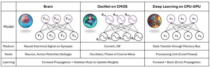
Figure 1: The Oscillator Network (OscNet) is a CMOS circuit inspired by the brain, where current serves as the medium for information transmission between oscillators. The network employs the Hebbian rule for learning, enabling adaptive and efficient connectivity among oscillators. Like the brain, OscNet calculates model responses and update weights with forward propagation only. Compared to recent deep learning models where back propagation is also needed, OscNet saves time and energy.

Machine learning, as the cornerstone of Artificial Intelligence (AI), has the capability to tackle a diverse array of significant challenges. Its applications [12, 11, 13, 10] span across critical domains such as healthcare [31, 68, 2], finance [22, 3, 28], and industry [6, 63]. However, with the development of AI, the time and energy costs associated with training models are becoming increasingly high and unsustainable [48, 5, 15, 21]. To save energy, there is an urgent need for new computational fabrics to replace the existing von Neumann architecture and CPU-GPU-based computation and training pipeline. Brain-inspired systems have become increasingly promising in recent years [16, 51], particularly Complementary Metal Oxide Semiconductor (CMOS) oscillator systems, which are being explored for optimization architectures [71]. These architectures have already been proven to solve some NP-hard problems, such as graph coloring, and can be applied in quantum computing gate emulation [72, 73].

In response to this, we propose a new and energy efficient computing and learning pipeline based CMOS Oscillator Networks (OscNet). OscNet computes with interactions between oscillators and learns with Hebbian rule. The advantages of OscNet include:

• OscNet is a brain-inspired computational architecture and is biologically meaningful. In this paper, OscNet is used to simulate the development of the human visual system before birth, specifically the process of establishing connections between retinal cells and lateral geniculate nucleus (LGN);

• In machine learning, we propose to update OscNet weights with forward propagation and Hebbian rule, eliminating the computational overhead of back propagation. It has similar or even higher performance with current deep learning pipelines and is energy efficient;

• From a hardware perspective, the integrated CMOS OscNet offers the benefits of compact area and compatibility with standard foundries, serving as a promising alternative to the von Neumann architecture.

In this paper, we propose the Multi-Input Multi-Output (MIMO) OscNet for image convolution, simulating the development of the human visual system before birth, where retinal cells and LGN neurons establish connections using Hebbian learning rules. We find that the Hebbian learning on MIMO OscNet is also suitable for unsupervised machine learning in Auto Encoder fashion, requiring only forward propagation and eliminating the time- and energy-consuming back propagation. OscNet is also specially designed to implement K-means. Furthermore, MIMO OscNet can be used for supervised linear regression. In all, the proposed inference and learning pipeline on OscNet is a promising alternative to current framework of machine learning on von Neumann architectures.

2 Proposed Model

2.1 OscNet and Potts Hamiltonian

CMOS Oscillator Network (OscNet) [72, 73, 71] operates with high-order injection locking, with local connections to neighboring oscillators. All oscillators are injected with a master pump signal at $N\textperiodcentered f_{0}$, where $f_{0}$ is oscillators’ natural oscillator frequency, and $N$ is a chosen integral. The phases of oscillators can be $n\frac{2\pi}{N}$, where $n=1,2...N-1$. This network mimics the activity of polychronous spiking neurons in the brain [40, 9], where each oscillator represents a single brain cell. In OscNet, all oscillators oscillate at the same frequency, and the information is encoded in the phases of the individual oscillators. The voltage across the oscillator $i$ at time $t$ is:

$$V_{i}(t)=A_{i}cos(\omega_{0}t+\theta_{i}),$$ (1)

where $\omega_{0}$ is the free-running frequency of the oscillator, $A_{i}$ is the amplitude, and $\theta_{i}$ is the phase. Each oscillator outputs a current based on its own state, while changes in its phase are determined by the influence of neighboring oscillators and the main pump, which can be explained by Impulse Sensitivity Function (ISF) theory [34, 70]. Phase changes of oscillator $i$ that is connected to neighboring oscillators can be represented by Kuramoto’s equation [65, 72]:

$$\frac{d\theta_{i}}{dt}=\sum_{(i,j)\in\mathcal{N}}K_{ij}sin(\theta_{i}-\theta_{j})+K_{p}sin(N\theta_{i}),$$ (2)

where $k_{i,j}$ represents the coupling strength between oscillator $i$ and $j$, $K_{p}$ models the main pump current and ISF, and $\mathcal{N}$ is the set of neighboring oscillators of $i$. The global Lyapunov function exists and will be minimized over time by the oscillator network [72, 33, 80]:

$$E(t)=\frac{N}{2}\sum_{(i,j)\in\mathcal{N}}K_{ij}cos(\theta_{i}-\theta_{j})+\sum_{i}K_{p}cos(N\theta_{i}).$$ (3)

Eq. 3 takes a similar form of Potts Hamiltonian [86]:

$$H=-\sum_{(i,j)\in\mathcal{N}}J_{ij}cos(\theta_{i}-\theta_{j})-\sum_{i}h_{i}.$$ (4)

Potts Hamiltonian was initially developed to model overall energy and phase transitions in ferromagnetic materials. The CMOS oscillator network can find the minimal value of Potts Hamiltonian and thus minimize energy of the system. In this paper, we model problems with Potts Hamiltonian, design structures of OscNet and it finds optimal phases of the system.

2.2 MIMO OscNet

We propose Multi-Input Multi-Output (MIMO) OscNet, which accepts data inputs and represents the data through the phases of oscillators. In the output layer, OscNet solves the system’s Potts Hamiltonian, achieving the same effect as the network’s forward propagation in current deep learning frameworks. The MIMO OscNet is shown in the middle of Fig. 1. Phases of input oscillators, denoted as $\theta_{i}$, are fixed, while the output layer oscillators, $\theta_{o}$, are free-running. The main pump of OscNet is $Nf_{0}$, and we assume that $N$ is infinite in this model. Thus the phases of oscillators can take any value in $[0,2\pi]$, and $cos(\theta-\theta_{i})$ can be anywhere between $-1$ and $1$. Each output oscillator $\theta_{oj}$ is influenced by the input data $\theta_{i}$ and the network connection weights, or more specifically, the coupling strength $w_{i,j}$ between the input and output oscillators. Additionally, there is no direct coupling between different output oscillators, such as $\theta_{oj_{1}}$ and $\theta_{oj_{2}}$, ensuring they do not interfere with each other. Since $J_{ij}$ can be either positive or negative, for simplicity, we ignore the negative sign in Eq. 8. $h_{i}$ is a time-independent term and can also be ignored in the differentiation. Consider an output oscillator $\theta_{o}$, its value is given by Potts Hamilton:

$$\theta_{oj}=argmin_{\theta}\>H=argmin_{\theta}\>\sum_{i=1}^{N}J_{ij}cos(\theta-\theta_{i}).$$ (5)

We igonre $h_{i}$ in Eq. 5 as it is independent of $\theta$. The Potts Hamilton can be solved by:

$$\frac{\partial H}{\partial\theta} =0$$ (6)

$$\frac{\partial H}{\partial\theta} =-\sum_{i=1}^{N}J_{ij}sin(\theta-\theta_{i})$$ (7)

$$=-\sum_{i=1}^{N}J_{ij}(sin\theta_{i}cos\theta-cos\theta_{i}sin\theta)$$

$$=-[cos\theta\sum_{i=1}^{N}J_{ij}sin\theta_{i}-sin\theta\sum_{i=1}^{N}J_{ij}cos\theta_{i}]$$

$$=\sqrt{(\sum_{i=1}^{N}J_{ij}sin\theta_{i})^{2}+(\sum_{i=1}^{N}J_{ij}cos\theta_{i})^{2}}sin(\theta-\theta_{0}),$$

So $\theta_{oj}$ is:

$$\theta_{oj}=\theta_{0}=arctan\frac{\sum_{i=1}^{N}J_{ij}sin\theta_{i}}{\sum_{i=1}^{N}J_{ij}cos\theta_{i}}.$$ (8)

MIMO OscNet has $N$ input oscillators and $M$ output oscillators. It is fully connected so there are $MN$ connections in total. Since the oscillators in the output layer do not interact with each other, the MIMO OscNet can be viewed as $M$ Multi-input Single-output OscNets sharing the same input but with different coupling strengths, simultaneously solving the Potts Hamiltonian. In the following chapters, we will demonstrate how MIMO OscNet can model biological development and solve machine learning problems.

3 Biological Views of OscNet

3.1 Image Convolution with OscNet

In image convolution, $I(x,y)$ and $I_{i}$ are pixel values at position $(x,y)$ and $i$. $I^{\prime}(x,y)$ is pixel value at position $(x,y)$, after convolution.

$$I^{\prime}(x,y)=\frac{\sum_{i=1}^{N}w_{i}I_{i}}{\sum_{i=1}^{N}w_{i}}.$$ (9)

Normalization is applied to Eq. 9. Gaussian blurring is a special case of convolution, where $w_{i}$ is sampled from a 2-dimensional Gaussian distribution. Considering Eq. 8 and Eq. 9 , we map:

$$w_{i}I_{i} =J_{i}sin\theta_{i},$$ (10)

$$w_{i} =J_{i}cos\theta_{i}.$$ (11)

So:

$$\theta_{i} =arctanI_{i},$$ (12)

$$J_{i} =\frac{w_{i}}{cos\theta_{i}}=w_{i}\sqrt{I_{i}^{2}+1}.$$ (13)

OscNet gives us $\theta=arctan\frac{\sum_{i=1}^{N}J_{i}sin\theta_{i}}{\sum_{i=1}^{N}J_{i}cos\theta_{i}}$, and $tan\theta$ is $I^{\prime}(x,y)$ after convolution (or blurring). By assigning appropriate coupling weights and phases to the input oscillators, the OscNet can automatically perform image convolution and blurring. The operation of OscNet for image convolution can be succinctly summarized as: given input pixels $I_{i}=tan\theta_{i}$, OscNet runs forward propagation once and we can read out from output oscillators that convoluted pixel is $I^{\prime}=tan\theta$. By using multiple output oscillators, we can perform image convolution in parallel.

3.2 Human Visual System Development

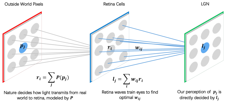
Figure 2: Modeling of human visual perception. Light from the real world travels to the retina, where it is processed by retina cells. These cells are densely connected to the LGN. The retina generates waves that help the brain optimize the weights $w_{ij}$ so that $l_{j}=p_{j}$, even without explicitly knowing the positions of the retina cells or having seen any real-world images beforehand.

In this section, we review the mechanisms of visual perception and the development of the visual system before birth, specifically the process of connecting the retina to the lateral geniculate nucleus (LGN) [14, 83, 50, 67]. When light enters the retinal cells, it is converted into electrical signals and then transmitted to the brain for processing. In digital images, pixels are evenly distributed along the x and y axes, but retinal cells are not uniformly distributed on the retina; instead, they are arranged in an irregular pattern. As a result, a straight line in the real world does not project as a straight line onto the retina. How do humans perceive a straight line as being straight?

The modeling of human perception of external light [62] is illustrated in Fig. 2. We model the real world as a set of pixels $p_{j}$ uniformly distributed along the x and y axes on a plane. According to the laws of light propagation, light from the outside world falls onto retinal cells, and the values of these retinal cells correspond to the intensity of the light received. The value of the retina cell $r_{i}$ is the summation of real-world pixels, under $P(p_{j})$, where $P$ models law of light transmission, effects of lens, and positional relationships between $p_{j}$ and $r_{i}$. Since the brain does not explicitly know the positions of retina cells, we do not explicitly know $P$. Retinal cells are densely connected to the LGN, where each LGN value represents a linear combination of values from several retinal cells. We assume that when the brain wants to know the value of pixels in a specific spatial location, it knows which LGN value to read. In other words, there exists a one-to-one mapping between LGN activity and the brain’s spatial perception. The value of LGN $l_{j}$ is decided by values of $r_{i}$ and connections $w_{ij}$ between retina cells and LGN, thus: $l_{j}=\sum_{i}w_{ij}r_{i}$. Therefore, the developmental process of the retinal-LGN connection can be formulated as an optimization problem:

$$\text{Find }w_{ij},\quad\text{so that }l_{j}=p_{j},$$ (14)

$$\text{s.t.}\quad l_{j}=\sum_{i}w_{ij}r_{i},$$

$$\quad\quad r_{i}=\sum_{j}P(p_{j}).$$

Before birth, the visual system undergoes preliminary development. The brain spontaneously generates retinal waves [4, 25, 26, 20, 43, 24], which act as a training signal to establish the correct connections between retinal cells and LGN. As a result, even before experiencing real-world images, the brain already knows that a straight line is straight. This developmental process can be effectively modeled using OscNet.

3.3 OscNet Modeling of Visual System

In the human visual system, transmission of information between retinal cells and the LGN can be seen as image convolution, where pixel values undergo a weighted average. Therefore, we can use forward propagation and Hebbian weight updating on OscNet to simulate how humans learn the connection weights between retinal cells and the LGN through retinal waves before birth. In OscNet, we use $tan\theta$ to represent numerical values, where $\theta$ is the phase of an oscillator. As shown in Algorithm 1, the Hebbian learning process involves updating retinal waves, performing forward propagation, and adjusting weights.

Algorithm 1 Hebbian Learning in OscNet with Retinal Waves

1:Initialize:

2:Fully connect retinal cells and LGN oscillators with randomly initialized connection weights.

3:for $i=1$ to $L$ do

4:  (a) Update retinal waves.

5:  (b) Perform OscNet forward propagation to compute LGN responses to retinal waves.

6:  (c) Read out values from LGN oscillators.

7:  (d) Update connection weights according to the Winner-Takes-All Hebbian rule.

8:end for

Compared to simulating this process on a von Neumann Architecture (VNA) computer, OscNet requires significantly fewer computational resources. With $n$ retinal cells and $m$ LGN neurons, VNA needs $nm$ computations to forward propagate, whereas OscNet achieves this in a single step.

Compared to deep learning, OscNet more closely aligns with biological development because:

• Forward propagation only: OscNet relies solely on forward propagation, mirroring brain development, whereas deep learning requires both forward and backward propagation;

• Local weight updates: In OscNet, weight updates depend only on local information. In biology, synaptic updates are influenced by the activities of the presynaptic and postsynaptic neurons. In contrast, deep learning’s weight updates depend on labels and the activities of neurons in higher layers of the network;

• Unsupervised learning in early visual system development: In the biological visual system, the retina-LGN pathway develops before birth, long before exposure to real-world images. The brain forms structures capable of perceiving a straight line as a straight line without ever having “seen” one. This process resembles unsupervised learning. In comparison, deep learning typically relies on supervised training.

4 Classification with OscNet

4.1 Auto Encoder with Hebbian Learning

In this section, we use MIMO OscNet for unsupervised Hebbian learning, like an AutoEncoder [59, 76, 87]. AutoEncoders utilize forward and backward propagation to update network weights, compressing input data into a specified dimension for efficient data encoding and representation. In contrast, OscNet requires only forward propagation to update weights and learn data features. It achieves results comparable to an AutoEncoder while being more energy-efficient, time-saving, and closely aligned with the brain’s natural learning process. The trained OscNet is then utilized for unsupervised classification and regression tasks. Additionally, we introduce a supervised linear transformation layer to refine the learned representations, following an unsupervised-pretraining and supervised-finetuning fashion.

Similar to Retina-LGN development in Algorithm 1, we update OscNet weights with Hebbian rule. MIMO OscNet has $N$ input and $M$ output oscillators with weight matrix $W_{ij}$, where $i\in[1,N]$ and $j\in[1,M]$. Given training data $(X)$, where $X$ is a feature vector of $N$ components. We assign input oscillator $i$ to phase $\theta_{i}=arctanX_{i}$. $X$ is forward propagated, so output oscillator $j$ will be

$$\theta_{j}=arctan\frac{\sum_{i=1}^{N}W_{ij}X_{i}}{\sum_{i=1}^{N}W_{ij}}.$$ (15)

We choose $j^{*}$ so that:

$$j^{*}=argmax_{j}tan\theta_{j}.$$ (16)

According to Hebbian rule, when an axon of cell A is near enough to excite a cell B and repeatedly or persistently takes part in firing it, some growth process or metabolic change takes place in one or both cells such that A’s efficiency, as one of the cells firing B, is increased [32]. Winner-Takes-All (WTA) strategy is adopted. We increase connections between the maximum $tanj$ and input oscillators, while other connections fade. The overall weight updating strategy is:

$$\text{Update}(W_{ij})=\begin{cases}W_{ij}+\tan\theta_{j^{*}}(X-\tan\theta_{j^{*}}W_{ij}),&j=j^{*},\\ W_{ij}-\lambda\tan\theta_{j^{*}}(X-\tan\theta_{j^{*}}W_{ij}),&j\neq j^{*},\end{cases}$$ (17)

where $\lambda$ is a coefficient that controls the rate at which the weights decay. In this way, OscNet learns features in the dataset in a unsupervised manner that aligns with brain development principles. The learned OscNet is ready for unsupervised classification and regression. Additional, OscNet can be used to train an additional linear regression layer in a supervised manner. This linear layer performs a weighted combination of the learned features to improve prediction accuracy. Fine-tuning involves only the linear regression layer, resulting in minimal parameters and low resource consumption. This approach of unsupervised pretraining followed by supervised finetuning [23, 60] is widely adopted in modern deep learning frameworks.

4.2 OscNet K-means

Given input $x_{i}$ and network weight $w_{ij}$, the output of OscNet $y_{j}$ can be written as:

$$y_{j}=\sum_{i}x_{i}w_{ij}=\mathbf{w}_{j}\cdot\mathbf{x}.$$ (18)

For OscNet Hebbian learning in clustering, a data point is clustered to class $j^{*}$ if $y_{j^{*}}=max_{j}y_{j}$. According to Eq. 18, we can define the overall energy term (or error) as the relative number of cosine similarity [36]. Thus the center of a class $C_{j}$ is ideally:

$$\mathbf{w}_{j}=\sum_{\mathbf{x}\in C_{j}}\frac{\sum\mathbf{x}}{\|\mathbf{x}\|}.$$ (19)

In OscNet, we use weight $\mathbf{w}_{j}$ to represent center of cluster $C_{j}$. Given input data $\mathbf{x}$ and current network weight $\mathbf{w}$, forward propagation of OscNet finds the cluster $\mathbf{x}$ belongs to by checking the maximum output oscillator. Thus we can use OscNet for K-means. OscNet only needs to run once to determine which cluster the data belongs to. Compared to calculating distances multiple times on a CPU, it saves both time and energy.

5 Regression with OscNet

In this section, we describe supervised learning using OscNet. Specifically, we apply OscNet to linear regression, where an analytical solution exists. Since nonlinear regression problems can be transformed into linear ones using polynomial transformations [57, 77], SVM [84, 74, 19], and kernels [69, 56, 82], the proposed OscNet can be applied to a broader range of regression problems.

5.1 Single Variable Linear Regression

We start with a single variable object function. The training data is denoted as $(x_{i},y_{i})$, $i=1,2,...N$ where $N$ is the number of training data. We aim to fit $f(x)=kx$ on the training data. The objective can be written as minimizing Mean Squared Error (MSE) loss:

$$l(k)=\sum_{i=1}^{N}(kx_{i}-y_{i})^{2}.$$ (20)

To find $k=argmin_{k}l(k)$, we compute the derivative of $l(k)$:

$$\frac{\partial l(k)}{\partial k} =\frac{2}{N}\sum_{i=1}^{N}(x_{i}^{2}k-x_{i}y_{i})=0.$$ (21)

Thus:

$$k=\frac{\sum_{i=1}^{N}x_{i}y_{i}}{\sum_{i=1}^{N}x_{i}^{2}}.$$ (22)

Comparing Eq. 22 and Eq. 8, we cast the regression problem to Potts Hamilton by:

$$x_{i}y_{i} =J_{i}sin\theta_{i},$$ (23)

$$x_{i}^{2} =J_{i}cos\theta_{i}.$$ (24)

This gives:

$$\theta_{i} =arctan\frac{y_{i}}{x_{i}},$$ (25)

$$J_{i} =\frac{x_{i}^{2}}{cos\theta_{i}}=x_{i}\sqrt{x_{i}^{2}+y_{i}^{2}}.$$ (26)

We can set the coupling strength following Eq. 25 and Eq. 26, so OscNet can find the solution $k$ to linear regression, according to Eq. 22

5.2 Multivariable Regression with Coordinate Descent

We focus on multivariable linear regression with coordinate descent. Coordinate Descent minimizes loss by iteratively minimizing a multivariable function along one coordinate direction at a time while keeping other variables fixed, which is commonly used in machine learning and statistics for solving regression problems. Please note that a lot of regression problem can be rewritten into linear regression. For example, $\theta_{1}x^{2}+\theta_{2}x$ can be rewritten into $\theta_{1}x_{1}+\theta_{2}x_{2}$. In kernel regression, we use kernel $\phi(x)$ and solve $f(\phi(\mathbf{x}))=\sum_{i=1}^{N}(\theta_{i}\phi_{i}(\mathbf{x}))+\theta_{0}$. It is also important to note that linear regression is a single-layer neural network in deep learning.

On training data $(\mathbf{x_{i}},y_{i})=(x_{i1},x_{i2},...,x_{iM},y_{i})$ where $i=1,2...N$, we aim to fit $f(\mathbf{\theta},\mathbf{x})=\theta_{0}+\sum_{k=1}^{M}\theta_{k}x_{k}$. The MSE loss function is:

$$l(\mathbf{\theta})=l(\theta_{0},\theta_{1},\theta_{2},...\theta_{m})=\sum_{i=1}^{N}(\theta_{0}+\sum_{k=1}^{M}\theta_{k}x_{ik}-y_{i})^{2}.$$ (27)

In coordinate descent, we choose $\theta_{j}$, fix every other $\theta_{k}$ ($k\neq j$), and find $\theta_{j}$ to minimize $l(\mathbf{\theta})$. So loss can be rewritten into:

$$l(\mathbf{\theta})=l(\theta_{j})=\sum_{i=1}^{N}(\theta_{j}x_{ij}-h_{i})^{2},$$ (28)

where $h_{i}=y_{i}-\theta_{0}-\sum_{k=1,i\neq j}^{M}\theta_{k}x_{k}$ is a constant, given that we fix every $\theta_{k}(k\neq j)$ and know $(\mathbf{x_{i}},y_{i})$ from training data. Eq. 28 is exactly the same with single variable regression Eq. 20. In coordinate descent, we iteratively choose $j$ and update$\theta_{j}$ until the loss function converges to a locally optimal value.

6 Simulations

To verify the effectiveness of OscNet at the circuit level, we simulate MIMO OscNet using MATLAB [39], based on Kuramoto’s equation [65]. Given the network structure, coupling strength, and the phase of the input oscillator, we observe the phase of the free-running oscillators, which serves as the output.

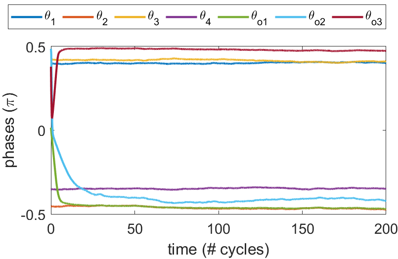
Figure 3: MIMO OscNet simulation for 4 inputs and 3 outputs.

We simulate MIMO OscNet with $N=4$ input oscillators and $M=3$ outputs. Each row represents an input oscillator $\theta_{i}$, and each column is an output oscillator $\theta_{j}$. Input numerical values are $X=[3,-7,4,-2]$, and encoded to $\theta=[0.397\pi,-0.455\pi,0.422\pi,-0.352\pi]$ following Eq. 12. The weights matrix is:

$$W=\begin{bmatrix}-3&-9&0\\ 8&2&-6\\ -1&7&10\\ 7&5&-1\end{bmatrix},$$ (29)

In OscNet, the weights of oscillator connections are encoded following Eq. 13. As shown in Fig. 3, OscNet finds phases of output oscillators to be $\theta_{o}=[-0.458\pi,-0.432\pi,0.489\pi]$, which corresponds to $O=[-7.545,-4.600,28.000]$. The simulation results agree with the theory.

7 Experiments

In the previous section, we validated the feasibility of MIMO OscNet. In this section, we use an unsupervised pretrained OscNet to perform unsupervised tasks followed by supervised fine-tuning.

7.1 Unsupervised Classification

We use the handwritten digit classification dataset MNIST. The number of input features is $N=784$, and the output has $M=10$ classes. We train the network using the Hebbian rule to update the weights. During the testing phase, given an input image, after forward propagation, if output oscillator $j$ exhibits the maximum response, we classify the image as belonging to class $j$. As a comparison, we also use an AutoEncoder [59, 76, 87]. The AutoEncoder has $N$ input nodes, $M$ hidden nodes in one layer, and $N$ output nodes, trained using error propagation. However, the performance of a single hidden-layer AutoEncoder is suboptimal. Therefore, we also include a two-hidden-layer AutoEncoder for comparison, where the two hidden layers have 128 and 10 nodes, respectively. Experimental results are shown in Table. 1. OscNet with Hebbian learning reaches a much higher accuracy than AutoEncoders. The learned features of OscNet and AutoEncoder are shown in Fig. 4. Please note that this is just a fully connected network, without using priors such as convolutional kernels. The receptive field corresponding to each hidden neuron is autonomously learned during training.

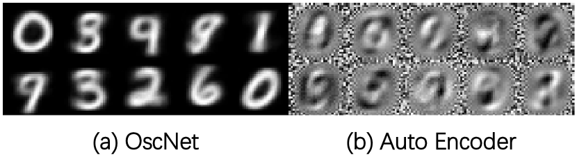
Figure 4: Learned features of OscNet and Auto Encoder on MNIST with 10 hidden neurons.

Table 1: Accuracy of OscNet and AutoEncoders on MNIST test set. Models are all trained on MNIST train set in a unsupervised manner.

Model	Accuracy (%)
AutoEncoder - 1 Hidden Layer	13.77
AutoEncoder - 2 Hidden Layer	28.72
OscNet (Ours)	57.31

7.2 Supervised Finetuning

After unsupervised pretraining of OscNet, we perform supervised training of a linear regression layer on the learned features and test the classification accuracy on MNIST. Experimental results are shown in Table. 2. Compared to the deep learning pipeline where an Auto Encoder-Auto Decoder structure is pretrained and a linear regression layer is fine-tuned on the AutoEncoder in a supervised manner, OscNet excels at more extreme data compression. With fewer hidden neurons, OscNet achieves higher accuracy, demonstrating superior compression and feature extraction. When the hidden layer size increases, OscNet achieves results comparable to those of the Auto Encoder. This suggests that OscNet, as a more energy-efficient pipeline, has the potential to replace existing machine learning frameworks without compromising accuracy or performance.

Table 2: OscNet and Hebbian rule pretraining, followed by finetuning a linear regression layer on MNIST. Auto Encoder pretraining - linear regression finetuing is the baseline, which is trained on error back propagation.

Model	# Hidden Neurons	Accuracy (%)
AutoEncoder	10	73.84
OscNet (Ours)	10	77.47
AutoEncoder	16	81.22
OscNet (Ours)	16	85.61
AutoEncoder	64	89.96
OscNet (Ours)	64	90.58
AutoEncoder	128	91.35
OscNet (Ours)	128	91.33

7.3 OscNet K-means

The experimental results of OscNet K-means is shown in Table. 3. OscNet with cosine similarity reaches almost same performance than K-means with Euclidean distance error implemented on CPU.

Table 3: K-means compared with OscNet K-means on MNIST.

Model	Accuracy (%)
K-means	59.46
OscNet K-means	60.84

8 Related Work

8.1 Polychronous Oscillatory Networks

The Ising model [79, 78, 38, 17] was discovered in the context of ferromagnetism in statistical mechanics. The Ising Machine leverages the natural tendency of such systems to minimize their energy, enabling it to efficiently find optimal solutions [53, 47, 18, 42]. It has been widely applied to various combinatorial optimization problems. In an Ising Machine, each node can only exist in one of two possible states. In this paper, we build upon the principles of CMOS oscillator networks and the Ising Machine to design a system capable of converging to the minimum of the Potts Hamiltonian, where each node can have multiple states. Polychronous Oscillator Networks on CMOS are inspired by spiking neurons, mimicking their interactions, and have been successfully applied to NP-hard problems such as Graph Coloring, as well as in designing quantum computers. Inspired by neural computing [66, 85, 64, 81] and their implementation on hardware [49, 35, 46], we design a MIMO OscNet structure, where some oscillators serve as inputs and others as outputs. The hardware can autonomously perform inference, effectively enabling forward propagation. The primary goal of this paper is to design an appropriate learning strategy to complement this hardware, enabling its application in machine learning tasks.

8.2 Hebbian Learning

Biological systems learn through signal forward propagation and Hebbian learning [29, 1]. In essence, Hebbian theory states that an increase in synaptic efficacy arises from the repeated and persistent stimulation of a postsynaptic cell by a presynaptic cell [8, 55]. Before birth, humans undergo initial learning of the visual system spontaneously. Retinal waves [4, 25, 26, 20, 43, 24, 37] are generated on the retina as input signals, and the connection weights between retinal cells and the LGN are updated based on Hebbian theory [62]. Similar learning mechanisms, rooted in Hebbian learning [27], are also applied in principal component analysis (PCA) [45], sparse coding [7], reinforcement learning [75, 61] and unsupervised learning in neural networks [44, 41, 54, 52, 30, 58]. Using the Winner-Takes-All (WTA) strategy, network weights are updated efficiently. In this paper, we model the early visual system development using Hebbian theory and OscNet to address the question: How do humans perceive a straight line as being straight in Sec. 3.2. We design a pipeline where forward propagation and Hebbian weight updating serve as the foundation for OscNet’s unsupervised learning. This pipeline demonstrates its applicability not only in unsupervised learning tasks but also in general supervised machine learning tasks.

9 Conclusion

In this paper, we propose OscNet, an energy-efficient machine learning framework based on CMOS oscillators. OscNet leverages interactions of oscillators to achieve minimization of Potts Hamiltonian. Compared to traditional deep learning architectures, OscNet more closely mirrors the structure of the human brain while being significantly more energy-efficient. We introduce a phase-based representation for numerical values in OscNet, applying it to machine learning tasks where solving the Potts Hamiltonian corresponds to forward propagation. Inspired by Hebbian learning in the human brain, we use OscNet to model the development of the prenatal human visual system and extend this model to unsupervised network pre-training. A trained OscNet can perform unsupervised classification in Auto Encoder or K-means fashion or be fine-tuned in a supervised manner with an additional layer. These promising features suggest that OscNet has the potential to become a computational fabric for next-generation AI systems.

References

- [1] Adams, P.: Hebb and darwin. Journal of theoretical Biology 195(4), 419–438 (1998)
- [2] Ahmad, M.A., Eckert, C., Teredesai, A.: Interpretable machine learning in healthcare. In: Proceedings of the 2018 ACM international conference on bioinformatics, computational biology, and health informatics. pp. 559–560 (2018)
- [3] Ahmed, S., Alshater, M.M., El Ammari, A., Hammami, H.: Artificial intelligence and machine learning in finance: A bibliometric review. Research in International Business and Finance 61, 101646 (2022)
- [4] Albert, M.V., Schnabel, A., Field, D.J.: Innate visual learning through spontaneous activity patterns. PLoS Computational Biology 4 (2008), https://api.semanticscholar.org/CorpusID:1493332
- [5] Bannour, N., Ghannay, S., Névéol, A., Ligozat, A.L.: Evaluating the carbon footprint of nlp methods: a survey and analysis of existing tools. In: Proceedings of the second workshop on simple and efficient natural language processing. pp. 11–21 (2021)
- [6] Bertolini, M., Mezzogori, D., Neroni, M., Zammori, F.: Machine learning for industrial applications: A comprehensive literature review. Expert Systems with Applications 175, 114820 (2021)
- [7] Boutin, V., Franciosini, A., Ruffier, F., Perrinet, L.: Effect of top-down connections in hierarchical sparse coding. Neural Computation 32(11), 2279–2309 (2020)
- [8] Brown, T.H., Kairiss, E.W., Keenan, C.L.: Hebbian synapses: biophysical mechanisms and algorithms. Annual review of neuroscience 13(1), 475–511 (1990)
- [9] Buzsáki, G., Draguhn, A.: Neuronal oscillations in cortical networks. Science 304, 1926 – 1929 (2004), https://api.semanticscholar.org/CorpusID:8002293
- [10] Cai, W., Hu, D., Yin, R., Deng, J., Fu, H., Yang, W., Gong, M.: Uncertainty quantification in stereo matching. arXiv preprint arXiv:2412.18703 (2024)
- [11] Cai, W., Jin, K., Hou, J., Guo, C., Wu, L., Yang, W.: Vdd: Varied drone dataset for semantic segmentation. arXiv preprint arXiv:2305.13608 (2023)
- [12] Cai, W., Ponomarenko, I., Yuan, J., Li, X., Yang, W., Dong, H., Zhao, B.: Spatialbot: Precise spatial understanding with vision language models. arXiv preprint arXiv:2406.13642 (2024)
- [13] Cai, W., Yang, W.: Object-level geometric structure preserving for natural image stitching. arXiv preprint arXiv:2402.12677 (2024)
- [14] Chapman, B., Stryker, M.P.: Development of orientation selectivity in ferret visual cortex and effects of deprivation. In: Journal of Neuroscience (1993), https://api.semanticscholar.org/CorpusID:1562405
- [15] Chien, A.A., Lin, L., Nguyen, H., Rao, V., Sharma, T., Wijayawardana, R.: Reducing the carbon impact of generative ai inference (today and in 2035). In: Proceedings of the 2nd workshop on sustainable computer systems. pp. 1–7 (2023)
- [16] Choudhary, S., Sloan, S., Fok, S., Neckar, A., Trautmann, E., Gao, P., Stewart, T., Eliasmith, C., Boahen, K.: Silicon neurons that compute. In: Artificial Neural Networks and Machine Learning–ICANN 2012: 22nd International Conference on Artificial Neural Networks, Lausanne, Switzerland, September 11-14, 2012, Proceedings, Part I 22. pp. 121–128. Springer (2012)
- [17] Cipra, B.A.: An introduction to the ising model. The American Mathematical Monthly 94(10), 937–959 (1987)
- [18] Cipra, B.A.: The ising model is np-complete. SIAM News 33(6), 1–3 (2000)
- [19] Cortes, C., Vapnik, V.N.: Support-vector networks. Machine Learning 20, 273–297 (1995), https://api.semanticscholar.org/CorpusID:52874011
- [20] Dähne, S., Wilbert, N., Wiskott, L.: Slow feature analysis on retinal waves leads to v1 complex cells. PLoS computational biology 10(5), e1003564 (2014)
- [21] Desislavov, R., Martínez-Plumed, F., Hernández-Orallo, J.: Compute and energy consumption trends in deep learning inference. arXiv preprint arXiv:2109.05472 (2021)
- [22] Dixon, M.F., Halperin, I., Bilokon, P.: Machine learning in finance, vol. 1170. Springer (2020)
- [23] Erhan, D., Courville, A., Bengio, Y., Vincent, P.: Why does unsupervised pre-training help deep learning? In: Proceedings of the thirteenth international conference on artificial intelligence and statistics. pp. 201–208. JMLR Workshop and Conference Proceedings (2010)
- [24] Feller, M., Kerschensteiner, D.: Retinal waves and their role in visual system development. In: Synapse development and maturation, pp. 367–382. Elsevier (2020)
- [25] Firth, S.I., Wang, C.T., Feller, M.B.: Retinal waves: mechanisms and function in visual system development. Cell calcium 37(5), 425–432 (2005)
- [26] Ge, X., Zhang, K., Gribizis, A., Hamodi, A.S., Sabino, A.M., Crair, M.C.: Retinal waves prime visual motion detection by simulating future optic flow. Science 373(6553), eabd0830 (2021)
- [27] Gerstner, W., Kistler, W.M.: Mathematical formulations of hebbian learning. Biological cybernetics 87(5), 404–415 (2002)
- [28] Goodell, J.W., Kumar, S., Lim, W.M., Pattnaik, D.: Artificial intelligence and machine learning in finance: Identifying foundations, themes, and research clusters from bibliometric analysis. Journal of Behavioral and Experimental Finance 32, 100577 (2021)
- [29] Grossberg, S.: Adaptive pattern classification and universal recoding: I. parallel development and coding of neural feature detectors. Biological cybernetics 23(3), 121–134 (1976)
- [30] Gupta, M., Ambikapathi, A., Ramasamy, S.: Hebbnet: A simplified hebbian learning framework to do biologically plausible learning. In: ICASSP 2021-2021 IEEE International Conference on Acoustics, Speech and Signal Processing (ICASSP). pp. 3115–3119. IEEE (2021)
- [31] Habehh, H., Gohel, S.: Machine learning in healthcare. Current genomics 22(4), 291 (2021)
- [32] Hebb, D.O.: The organization of behavior: A neuropsychological theory. Psychology press (2005)
- [33] van Hemmen, J.L., Wreszinski, W.F.: Lyapunov function for the kuramoto model of nonlinearly coupled oscillators. Journal of Statistical Physics 72, 145–166 (1993), https://api.semanticscholar.org/CorpusID:122867392
- [34] Hong, B., Hajimiri, A.: A general theory of injection locking and pulling in electrical oscillators—part i: Time-synchronous modeling and injection waveform design. IEEE Journal of Solid-State Circuits 54, 2109–2121 (2019), https://api.semanticscholar.org/CorpusID:198356617
- [35] Hoppensteadt, F.C., Izhikevich, E.M.: Pattern recognition via synchronization in phase-locked loop neural networks. IEEE Transactions on Neural Networks 11(3), 734–738 (2000)
- [36] Hu, X., Zhang, J., Qi, P., Zhang, B.: Modeling response properties of v2 neurons using a hierarchical k-means model. Neurocomputing 134, 198–205 (2014)
- [37] Hunt, J.J., Ibbotson, M., Goodhill, G.J.: Sparse coding on the spot: Spontaneous retinal waves suffice for orientation selectivity. Neural computation 24(9), 2422–2433 (2012)
- [38] Inagaki, T., Haribara, Y., Igarashi, K., Sonobe, T., Tamate, S., Honjo, T., Marandi, A., McMahon, P.L., Umeki, T., Enbutsu, K., et al.: A coherent ising machine for 2000-node optimization problems. Science 354(6312), 603–606 (2016)
- [39] Inc., T.M.: Matlab version: 9.13.0 (r2022b) (2022), https://www.mathworks.com
- [40] Izhikevich, E.M., Hoppensteadt, F.C.: Polychronous wavefront computations. Int. J. Bifurc. Chaos 19, 1733–1739 (2009), https://api.semanticscholar.org/CorpusID:18305391
- [41] Journé, A., Rodriguez, H.G., Guo, Q., Moraitis, T.: Hebbian deep learning without feedback. arXiv preprint arXiv:2209.11883 (2022)
- [42] Kazakov, V.A.: Ising model on a dynamical planar random lattice: exact solution. Physics Letters A 119(3), 140–144 (1986)
- [43] Kim, J., Song, M., Jang, J., Paik, S.B.: Spontaneous retinal waves can generate long-range horizontal connectivity in visual cortex. Journal of Neuroscience 40(34), 6584–6599 (2020)
- [44] Krotov, D., Hopfield, J.J.: Unsupervised learning by competing hidden units. Proceedings of the National Academy of Sciences 116(16), 7723–7731 (2019)
- [45] Lagani, G., Amato, G., Falchi, F., Gennaro, C.: Training convolutional neural networks with hebbian principal component analysis. arXiv preprint arXiv:2012.12229 (2020)
- [46] Lopez-Pastor, V., Marquardt, F.: Self-learning machines based on hamiltonian echo backpropagation. Physical Review X 13(3), 031020 (2023)
- [47] Lucas, A.: Ising formulations of many np problems. Frontiers in physics 2, 5 (2014)
- [48] Luccioni, S., Jernite, Y., Strubell, E.: Power hungry processing: Watts driving the cost of ai deployment? In: The 2024 ACM Conference on Fairness, Accountability, and Transparency. pp. 85–99 (2024)
- [49] Maffezzoni, P., Bahr, B., Zhang, Z., Daniel, L.: Oscillator array models for associative memory and pattern recognition. IEEE Transactions on Circuits and Systems I: Regular Papers 62(6), 1591–1598 (2015)
- [50] Manganaro, G.: Another look at cellular neural networks. 2021 17th International Workshop on Cellular Nanoscale Networks and their Applications (CNNA) pp. 1–4 (2021), https://api.semanticscholar.org/CorpusID:244663050
- [51] Mead, C., Ismail, M.: Analog VLSI implementation of neural systems, vol. 80. Springer Science & Business Media (2012)
- [52] Miconi, T.: Hebbian learning with gradients: Hebbian convolutional neural networks with modern deep learning frameworks. arXiv preprint arXiv:2107.01729 (2021)
- [53] Mohseni, N., McMahon, P.L., Byrnes, T.: Ising machines as hardware solvers of combinatorial optimization problems. Nature Reviews Physics 4(6), 363–379 (2022)
- [54] Moraitis, T., Toichkin, D., Journé, A., Chua, Y., Guo, Q.: Softhebb: Bayesian inference in unsupervised hebbian soft winner-take-all networks. Neuromorphic Computing and Engineering 2(4), 044017 (2022)
- [55] Munakata, Y., Pfaffly, J.: Hebbian learning and development. Developmental science 7(2), 141–148 (2004)
- [56] Nadaraya, E.A.: On estimating regression. Theory of Probability & Its Applications 9(1), 141–142 (1964)
- [57] Neal, R.M.: Pattern recognition and machine learning, by christopher m. bishop. Technometrics 49 (2007), https://api.semanticscholar.org/CorpusID:262612365
- [58] Network, F.N.: Optimal unsupervised learning in a single-layer linear. Neural Networks 2, 459–473 (1989)
- [59] Ng, A., et al.: Sparse autoencoder. CS294A Lecture notes 72(2011), 1–19 (2011)
- [60] Paine, T.L., Khorrami, P., Han, W., Huang, T.S.: An analysis of unsupervised pre-training in light of recent advances. arXiv preprint arXiv:1412.6597 (2014)
- [61] Pugh, J., Soltoggio, A., Stanley, K.: Real-time hebbian learning from autoencoder features for control tasks. In: Artificial Life Conference Proceedings. pp. 202–209. MIT Press One Rogers Street, Cambridge, MA 02142-1209, USA journals-info … (2014)
- [62] Raghavan, G., Thomson, M.: Neural networks grown and self-organized by noise. In: Neural Information Processing Systems (2019), https://api.semanticscholar.org/CorpusID:174798065
- [63] Rai, R., Tiwari, M.K., Ivanov, D., Dolgui, A.: Machine learning in manufacturing and industry 4.0 applications (2021)
- [64] Ramasubramanian, S.G., Venkatesan, R., Sharad, M., Roy, K., Raghunathan, A.: Spindle: Spintronic deep learning engine for large-scale neuromorphic computing. In: Proceedings of the 2014 international symposium on Low power electronics and design. pp. 15–20 (2014)
- [65] Sakaguchi, H., Shinomoto, S., Kuramoto, Y.: Local and grobal self-entrainments in oscillator lattices. Progress of Theoretical Physics 77, 1005–1010 (1987), https://api.semanticscholar.org/CorpusID:122040965
- [66] Schuman, C.D., Potok, T.E., Patton, R.M., Birdwell, J.D., Dean, M.E., Rose, G.S., Plank, J.S.: A survey of neuromorphic computing and neural networks in hardware. arXiv preprint arXiv:1705.06963 (2017)
- [67] Sernagor, E., Mehta, V.: The role of early neural activity in the maturation of turtle retinal function. The Journal of Anatomy 199(4), 375–383 (2001)
- [68] Shailaja, K., Seetharamulu, B., Jabbar, M.: Machine learning in healthcare: A review. In: 2018 Second international conference on electronics, communication and aerospace technology (ICECA). pp. 910–914. IEEE (2018)
- [69] Shawe-Taylor, J., Cristianini, N.: Kernel methods for pattern analysis (2004), https://api.semanticscholar.org/CorpusID:35730151
- [70] Smith, R.L., Lee, T.H.: Hybrid frequency domain simulation method to speed-up analysis of injection locked oscillators. 2021 IEEE International Midwest Symposium on Circuits and Systems (MWSCAS) pp. 722–726 (2021), https://api.semanticscholar.org/CorpusID:237520896
- [71] Smith, R.L., Lee, T.H.: Modeling of injection locking in neurons for neuromorphic and biomedical systems. 2021 IEEE International Symposium on Circuits and Systems (ISCAS) pp. 1–5 (2021), https://api.semanticscholar.org/CorpusID:235566110
- [72] Smith, R.L., Lee, T.H.: Polychronous oscillatory cellular neural networks for solving graph coloring problems. IEEE Open Journal of Circuits and Systems 4, 156–164 (2023), https://api.semanticscholar.org/CorpusID:257796022
- [73] Smith, R.L., Lee, T.H.: Quantum computing gate emulation using cmos oscillatory cellular neural networks. IEEE Transactions on Circuits and Systems II: Express Briefs 71, 4541–4545 (2024), https://api.semanticscholar.org/CorpusID:269642781
- [74] Smola, A., Scholkopf, B.: A tutorial on support vector regression. Statistics and Computing 14, 199–222 (2004), https://api.semanticscholar.org/CorpusID:15475
- [75] Stanley, K., Pugh, J., Bowren, J.: Fully autonomous real-time autoencoder-augmented hebbian learning through the collection of novel experiences. In: ALIFE 2016, the Fifteenth International Conference on the Synthesis and Simulation of Living Systems. pp. 382–389. MIT Press (2016)
- [76] Tschannen, M., Bachem, O., Lucic, M.: Recent advances in autoencoder-based representation learning. arXiv preprint arXiv:1812.05069 (2018)
- [77] Vapni, V.N.: The nature of statistical learning theory. In: Statistics for Engineering and Information Science (2000), https://api.semanticscholar.org/CorpusID:7138354
- [78] Wang, T., Roychowdhury, J.: Oscillator-based ising machine. arXiv preprint arXiv:1709.08102 (2017)
- [79] Wang, T., Roychowdhury, J.: Oim: Oscillator-based ising machines for solving combinatorial optimisation problems. In: Unconventional Computation and Natural Computation: 18th International Conference, UCNC 2019, Tokyo, Japan, June 3–7, 2019, Proceedings 18. pp. 232–256. Springer (2019)
- [80] Wang, T., Roychowdhury, J.S.: Oim: Oscillator-based ising machines for solving combinatorial optimisation problems. In: International Conference on Unconventional Computation and Natural Computation (2019), https://api.semanticscholar.org/CorpusID:81979522
- [81] Wanjura, C.C., Marquardt, F.: Fully nonlinear neuromorphic computing with linear wave scattering. Nature Physics 20(9), 1434–1440 (2024)
- [82] Watson, G.S.: Smooth regression analysis. Sankhyā: The Indian Journal of Statistics, Series A pp. 359–372 (1964)
- [83] Wiesel, T.N., Hubel, D.H.: Ordered arrangement of orientation columns in monkeys lacking visual experience. Journal of Comparative Neurology 158 (1974), https://api.semanticscholar.org/CorpusID:42437417
- [84] Williams, C.K.I.: Learning with kernels: Support vector machines, regularization, optimization, and beyond. IEEE Transactions on Neural Networks 16, 781–781 (2003), https://api.semanticscholar.org/CorpusID:7406938
- [85] Wright, L.G., Onodera, T., Stein, M.M., Wang, T., Schachter, D.T., Hu, Z., McMahon, P.L.: Deep physical neural networks trained with backpropagation. Nature 601(7894), 549–555 (2022)
- [86] Wu, F.Y.: The potts model. Reviews of Modern Physics 54, 235–268 (1982), https://api.semanticscholar.org/CorpusID:120281979
- [87] Zhai, J., Zhang, S., Chen, J., He, Q.: Autoencoder and its various variants. In: 2018 IEEE international conference on systems, man, and cybernetics (SMC). pp. 415–419. IEEE (2018)