Online Aggregation of Trajectory Predictors

Abstract

Trajectory prediction, the task of forecasting future agent behavior from past data, is central to safe and efficient autonomous driving. A diverse set of methods (e.g., rule-based or learned with different architectures and datasets) have been proposed, yet it is often the case that the performance of these methods is sensitive to the deployment environment (e.g., how well the design rules model the environment, or how accurately the test data match the training data). Building upon the principled theory of online convex optimization but also going beyond convexity and stationarity, we present a lightweight and model-agnostic method to aggregate different trajectory predictors online. We propose treating each individual trajectory predictor as an “expert” and maintaining a probability vector to mix the outputs of different experts. Then, the key technical approach lies in leveraging online data –the true agent behavior to be revealed at the next timestep– to form a convex-or-nonconvex, stationary-or-dynamic loss function whose gradient steers the probability vector towards choosing the best mixture of experts. We instantiate this method to aggregate trajectory predictors trained on different cities in the nuScenes dataset and show that it performs just as well, if not better than, any singular model, even when deployed on the out-of-distribution Lyft dataset.

I Introduction

Predicting future trajectories of traffic agents is a central task in autonomous driving. Traditionally, rule-based methods were used for their simplicity, efficiency, and explainability [1, 2, 3]. In contrast, recent studies have shown that deep learning-based approaches [4, 5, 6] achieve superior performance due to their ability to learn spatial relationships and inter-agent dynamics from rich high-dimensional data.

However, each trajectory predictor is often trained on a specific dataset with a specific architecture, raising challenges when encountering new unseen datasets, as distribution shifts can significantly degrade a model’s test-time performance. A standard approach to mitigate this issue is data augmentation, i.e., combine all possible datasets and train a large model that hopefully becomes a generalist. While the promise of general foundational models trained from large datasets has (mostly) been fulfilled by large language and vision models [7], their out-of-distribution (OOD) generalization ability remains to be rigorously evaluated [8, 9, 10]. Moreover, in the context of trajectory prediction, it is unclear yet whether such a globally dominant model exists, as the distribution of future agent behavior can be heavily influenced by local traffic rules and driving norms across geographical locations.

In this paper, we explore the use of online aggregation of trajectory predictors as an alternative approach to out-of-distribution generalization. In statistical learning terms, our framework can be considered an example of boosting [11, 12]. Particularly, we treat each trajectory predictor as a black-box “expert” –whether the predictor was hand-crafted or learned, what architecture was used for learning, and which dataset it was trained on are all unknown to us– and use a probability vector to mix the outputs of different experts. The technical problem then becomes how to update the probability vector such that the mixture-of-experts (MoE) model remains robust to distribution shifts.

To solve this problem, we leverage theory from the emerging field of online convex optimization (OCO) [13]. In particular, OCO considers a dynamic game between a player and an adversarial environment. In each round $t$, the player outputs a decision $z_{t}$, the environment chooses a (potentially adversarial) convex loss function $l_{t}(z_{t})$ and reveals the gradient $g_{t}=\nabla l_{t}(z_{t})$. The goal of the player is to design an algorithm that takes in $g_{t}$ and outputs $z_{t}$ to minimize the notion of regret:

$$\mathrm{Regret}_{T}(l_{1:T},u):=\sum_{t=1}^{T}l_{t}(z_{t})-\sum_{t=1}^{T}l_{t}(u),$$ (1)

where $T$ is the horizon of the game and $u$ is any fixed comparator. Intuitively, we wish the regret to be sublinear in $T$, then the algorithm will converge to the best fixed decision in hindsight. Classical and recent literature in online learning established that gradient descent and its variants can indeed attain sublinear regret, see [13, 14] and references therein.

Contribution. We borrow the OCO framework to design a principled and lightweight framework for online aggregation of multiple trajectory predictors. We first assume the output of each trajectory predictor is a Gaussian mixture model (GMM). Then, using the OCO language presented above, the player’s decision $z_{t}$ is the probability vector, resulting in an MoE model that is a mixture of GMMs, which is a new GMM. The loss function $l_{t}$ uses the true agent state revealed at time $t$ to evaluate the performance of the MoE model. The player finally uses the gradient of $l_{t}$ to perform “online gradient descent” to update the probability vector. When the loss function is chosen as the negative probability loss, it becomes linear in $z_{t}$. In this case, the most well-known algorithm for online minimization of a linear function over $z_{t}$ (a probability vector) is called exponentiated gradient (EG) [13]. However, we found the empirical convergence rate of EG is too slow to be practical. To mitigate this issue, we depart from EG and choose the recent squint algorithm [15] with Cutkosky clipping [16] to update the probability vector online, which demonstrated roughly 25 times faster empirical convergence (see Appendix -A).

We then go beyond the convexity and stationarity assumptions in OCO and engineer two heuristics for a nonconvex loss function and nonstationary environments (i.e., the distribution shift happens more than once). First, when the loss function is chosen as the top-$k$ minimum first displacement error (minFRDE_k, a variant of a common performance metric in the literature), we approximate it using a differentiable surrogate [17] and then apply squint. Second, if the environment is nonstationary, we apply a discount factor when computing losses from previous steps [18], which allows the algorithm to gracefully forget the past and adapt to new distribution shifts.

To study the performance of our algorithm, we pretrain three trajectory predictors on the Boston, Singapore, and Las Vegas splits of the nuScenes dataset [19]. Together with a rule-based trajectory predictor [20], we perform online aggregation on two out-of-distribution datasets: (i) the Pittsburgh split of nuScenes and (ii) the Lyft dataset [21]. We show that the MoE model performs on par or better than any singular model on various performance metrics.

To summarize, our contributions are:

• We introduce a framework for online aggregation of multiple trajectory predictors to gain robustness against distribution shifts. Notably, our framework is agnostic to the design of individual predictors, as long as each of them outputs a distribution of trajectories.

• We apply the theory of online convex optimization to design a lightweight algorithm for online aggregation. Specifically, we identified that the classical EG algorithm in OCO is impractical for online aggregation in trajectory prediction, whereas the recent squint algorithm enables fast adaptation.

• We extend the OCO framework to handle nonconvexity and nonstationarity, allowing the online aggregation algorithm to optimize for diverse scenarios.

II Related Works

Trajectory Prediction. Early works on trajectory prediction focused on rule-based models, operating under the assumption that humans typically conform to a set of rules and customs [22]. However, the performance of rule-based predictors relies heavily on the completeness and soundness of the predefined rules. Furthermore, the “rigidity” of the rules can fail to capture the nuanced and stochastic nature of human driving, leading to an inability to reason about uncertainty and adapt to multimodal outcomes in complex interactions. Learning-based methods can address these limitations by leveraging data to train generative models [4, 5, 6] that reason about uncertainty and provide multimodal outcomes. Various architectures have been explored, e.g., recurrent neural networks (RNNs) [23, 24], transformers [6], variational auto-encoders (VAEs) [4], generative adversarial networks (GANs) [25], and even large language models (LLMs) [26].

Trajectory Predictor Fusion. Despite their ability to model uncertainty and multimodal behaviors, learned predictors often struggle to generalize to OOD scenarios, where the test distribution differs from the training data.

This has led to recent works combining rule-based and learned predictors in series [27, 28, 29] and in parallel [20, 30, 31]. While our proposed architecture is also in parallel, it does not use a Bayesian method for fusion and instead builds upon online convex optimization.

Online Learning in Robotics. A notable application of online convex optimization (OCO) in robotics is online control, which dates back to at least [32]. This approach reformulates online optimal control as an OCO problem, leveraging algorithmic insights from the OCO literature [33]. Building on these ideas, adaptive online learning has enabled parameter-free optimizers for lifelong reinforcement learning [34]. OCO has also proven valuable for online adaptive conformal prediction [35], where it helps construct prediction sets that guarantee coverage despite distribution shifts [18, 36]. Inspired by these successes, we investigate OCO’s application to aggregating trajectory predictors.

III Online Aggregation

In this section, we present our framework for online aggregation of trajectory predictors. We first define the problem setup (§III-A) and spend most of the content on presenting the algorithm for the case of convex loss and stationary environment (§III-B). After that, the extension to nonconvex loss and nonstationary environment becomes natural (§III-C and §III-D). Fig. 1 overviews our approach.

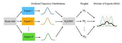
Figure 1: Online aggregation of trajectory predictors.

III-A Problem Setup

We are given $N$ trajectory predictors treated as black-box experts. We assume each trajectory predictor outputs a multimodal distribution parameterized as a categorical normal prediction, i.e., it predicts a probability vector $p\in\Delta_{L}$ over $L$ possible modes of future behavior. The $j$-th mode is modeled as a Gaussian distribution with mean $\mu_{j}\in\mathbb{R}^{K\times 3}$ (denoting the $xy$ position and heading $\theta$ of the agent in the next $K$ timesteps) and precision $h_{j}\in\mathbb{R}^{K\times 3}$ (e.g., $h_{j}(k,:)=[1/\sigma_{x}^{2},1/\sigma_{y}^{2},1/\sigma_{\theta}^{2}]^{T}$ represents the reciprocal of the variances in $x,y,\theta$ coordinates at the $k$-th prediction step). Let $\Sigma_{j}$ be the covariance matrix corresponding to $h_{j}$, we can write the output of the $i$-th predictor as a Gaussian Mixture Model (GMM):

$$\left\{(p_{1}^{i},\mu_{1}^{i},\Sigma_{1}^{i}),\cdots,(p_{L}^{i},\mu_{L}^{i},\Sigma_{L}^{i})\right\},\quad i=1,\dots,N$$ (2)

where $p^{i}_{j}\in\Delta_{L},\mu^{i}_{j}\in{{\mathbb{R}}^{K\times 3}},\Sigma_{j}^{i}\in(\mathbb{S}^{3}_{++})^{K},j=1,\dots,L$ ($\mathbb{S}^{3}_{++}$ denotes the set of $3\times 3$ positive definite matrices). Note that we use the superscript $i$ to index the $i$-th expert (trajectory predictor) and the subscript $j$ to index the $j$-th mode in the GMM.

Remark 1 (Generality).

In principle, our framework only requires each expert to output a distribution of trajectories that can be sampled from, and the distribution needs not be a GMM, see Appendix -D. Here we choose to present our framework by assuming each expert outputs a GMM for two reasons. (i) Many recent state-of-the-art trajectory predictors use GMMs to represent multimodal distributions, such as Trajectron++ [4], Wayformer [37], and MTR++ [38]. (ii) GMMs are easier to interpret than arbitrary distributions, and do not require sampling for online aggregation.

The Mixture-of-Experts Model. Given $N$ predictions of the form (2), we aggregate them by forming a mixture-of-experts (MoE) model. Particularly, the MoE model maintains a probability vector $\alpha\in\Delta_{N}$ where each $\alpha_{i}$ is used to weigh the importance of the $i$-th expert. Given $\alpha$, the MoE model outputs a new GMM model that is the mixture of $N\times L$ Gaussians

$$\Gamma(\alpha):=\left\{(\alpha_{i}p^{i}_{j},\mu^{i}_{j},\Sigma^{i}_{j})\right\}_{i=1,j=1}^{i=N,j=L}.$$ (3)

The goal of online aggregation is then to use online information to dynamically update $\alpha$.

III-B Convex Loss and Stationary Environment

We use OCO to update $\alpha$ in the MoE model (3). Let $\alpha_{t}$ be the probability vector “played” by the MoE model at time $t$, and $x_{t}\in{{\mathbb{R}}^{3}}$ be the true agent state revealed to the MoE model before it plays the next probability vector. A first choice for updating $\alpha_{t}$ given $x_{t}$ is to seek an $\alpha$ that maximizes the probability of $x_{t}$ given $\Gamma(\alpha_{t})$:

$$p(x_{t}|\Gamma(\alpha_{t}))=\sum_{i,j}\alpha_{i,t}p_{j,t}^{i}g(x_{t}|\mu^{i}_{j,t},\Sigma^{i}_{j,t})$$ (4)

where $g(x_{t}|\mu^{i}_{j,t},\Sigma^{i}_{j,t})$ denotes the probability density function (PDF) of a Gaussian distribution. In (4), we used the fact that the PDF of a GMM can be written as the weighted sum of the PDFs of its individual Gaussian components. Note that in (4) we added a subscript “$t$” to $(p,\mu,\Sigma)$ to make explicit their dependence on the time step. Finding the weights $\alpha$ that maximizes the probability $p(x_{t}|\Gamma(\alpha_{t}))$ is equivalent to finding the weights $\alpha$ that minimizes $-p(x_{t}|\Gamma(\alpha_{t}))$:

$$\ell_{t}(\alpha_{t})=-p(x_{t}|\Gamma(\alpha_{t})).$$ (5)

Clearly, the loss function is linear in $\alpha_{t}$ and its gradient with respect to $\alpha_{t}$ is

$$\nabla_{\alpha_{t,i}}\ell_{t}(\alpha_{t})=-\sum_{j}p^{i}_{j,t}g(x_{t}|\mu_{j,t}^{i},\Sigma^{i}_{j,t}),\ i=1,\dots,N.$$ (6)

The squint Algorithm. The de-facto algorithm for online minimization of the linear function $\ell_{t}(\alpha_{t})$ in (5) subject to $\alpha_{t}$ being a probability vector is the exponentiated gradient (EG) algorithm [13]. However, applying EG in the context of aggregating trajectory predictors is impractical because EG exhibits slow convergence (see Appendix -A for a description of the EG algorithm and results showing its slow convergence). To mitigate this issue, we introduce squint [15] as the algorithm to update $\alpha$, whose pseudocode is given in Algorithm 1 and follows the official implementation. Without going too deep into the theory, we provide some high-level insights.

• Goal of learning. Since the loss function is linear, the OCO problem reduces to hedging [39], or learning with expert advice [13]. In this setup, the $i$-th entry of the gradient ${g_{t}}\in{{\mathbb{R}}^{N}}$ in line 1 (for the discussion here let us first assume $g_{t}=\tilde{g}_{t}$) represents the loss of the $i$-th expert, for $i=1,\dots,N$. For online aggregation, one can check that the gradient in (6) represents the probability of $x_{t}$ under the $i$-th GMM and measures how well the $i$-th expert predicts the ground truth. By playing a MoE model using the probability vector $\alpha_{t}$, we suffer a weighted sum of individual expert losses, namely $\alpha_{t}^{\mathsf{T}}g_{t}$. The instantaneous regret $r_{t}$ defined in line 1 measures the relative performance of the MoE model with respect to each expert at time $t$, and the cumulative regret $R_{t}=\sum_{\tau=1}^{t}r_{t}$ computed in line 1 measures the relative performance over the time period until $T$. The goal of the learner (i.e., the MoE model) is to minimize each entry of $R_{t}$, i.e., to ensure that the regret with respect to any individual expert is small. By doing so, the learner is guaranteed to perform as well as the best expert (without knowing which expert is the best a priori).

• Bayes update. To achieve the goal of small regret, the squint algorithm essentially performs Bayes update. To see this, note that the algorithm starts with a prior distribution of expert weights $\alpha_{1}$, which represents the learner’s belief of which expert is the best, before receiving any online information. After the game starts, squint maintains the regret vector $R_{t}$, together with the cumulative regret squared vector $V_{t}=\sum_{\tau=1}^{t}r_{\tau}\circ r_{\tau}$ computed in line 1. The main update rule is written in (7) where the function $\xi(\cdot,\cdot)$ is a potential function called squint evidence. Note that the crucial difference between squint and the vanilla EG algorithm (see Appendix -A) is that squint uses second-order information, i.e., $V_{t}$. With this interpretation, we recognize (7) as an instance of Bayes’ rule with prior $\alpha_{1}$ and evidence measured by $\xi$. The detailed proof of why (7) guarantees small regret is presented in the original paper [15] and beyond the scope here due to its mathematical involvement.

• Gradient clipping   An assumption of the hedging setup is that individual expert losses need to be bounded, which may not hold for our problem. Therefore, in lines 1-1, we employ the gradient clipping method proposed in [16] to rescale the gradients. The gradient clipping technique has been a popular method in training deep neural networks [40, 41, 42].

Input: A prior distribution of the weights $\alpha_{1}$ for each expert

Initialize: Cumulative regret $R_{1}=0\in{{\mathbb{R}}^{N}}$, Cumulative regret squared $V_{1}=0\in{{\mathbb{R}}^{N}}$

1 for $t=1,2,\dots,T$ do

2    Compute $\ell_{t}$ as in (5) and define the gradient $\tilde{g}_{t}=\nabla_{\alpha_{t}}(\ell_{t})\in{{\mathbb{R}}^{N}}$

3   Set $G_{t}=\max(\max_{i\in[N]}(|\tilde{g}_{t,i}|),G_{t-1})$ ($\tilde{g}_{t,i}$ denotes the $i$-th element of $\tilde{g}_{t}$)

4   Define the clipped gradient $g_{t}=\frac{(\tilde{g}_{t}/G_{t})+1}{2}\in{{\mathbb{R}}^{N}}$ (element-wise division)

5   Define the instantaneous regret $r_{t}=\alpha_{t}^{\mathsf{T}}g_{t}-g_{t}\in{{\mathbb{R}}^{N}}$

6   Update

$$\alpha_{t+1,i}=\frac{\alpha_{1,i}\xi(R_{t,i},V_{t,i})}{\sum_{i}\alpha_{1,i}\xi(R_{t,i},V_{t,i})},\quad i=1,\dots,N$$ (7)

where

$$\hskip-11.38109pt\xi(R,V)=\sqrt{\pi}\exp{\left(\frac{R^{2}}{4V}\right)}\frac{\mathrm{erfc}(\frac{-R}{2\sqrt{V}})-\mathrm{erfc}(\frac{V-R}{2\sqrt{V}})}{2\sqrt{V}}$$ (8)

and $\mathrm{erfc}$ is the complementary error function $\mathrm{erfc}(x):=1-\frac{2}{\sqrt{\pi}}\int_{0}^{x}e^{-t^{2}}dt$

7   Update $R_{t+1}=R_{t}+r_{t}$ and $V_{t+1}=V_{t}+r_{t}\circ r_{t}$ (“$\circ$” denotes element-wise multiplication)

Algorithm 1 squint with Cutkosky Clipping

The squint algorithm guarantees sublinear regret [15, Theorem 4]. The loss function $\ell_{t}(\cdot)$ is linear in $\alpha$ and $\alpha$ lives in the probability simplex, which implies the optimal $\alpha$ in hindsight must be a one-hot vector that assigns $1$ to the best expert and $0$ to other experts [43]. Therefore, we conclude that squint guarantees convergence to the best expert in hindsight, as we will empirically show in §IV.

III-C Nonconvex Loss

The probability loss (5) intuitively considers the “average” performance of the MoE model in the sense that all the Gaussian modes are included (penalized) in computing the loss. In practice, however, we may not care about all modes of the MoE model but rather its top-$k$ modes. Formally, let $\alpha_{t}$ be the decision of the MoE model at time $t$ and denote $\phi_{t}=(\phi_{1,t},\dots,\phi_{k,t})\in[NL]$ as the indices of the top-$k$ modes in the MoE model (3)

$$\phi_{t}=(\phi_{1,t},\dots,\phi_{k,t})=\mathrm{argtopk}\{\alpha_{i,t}p^{i}_{j,t}\}_{i=1,j=1}^{i=N,j=L},$$ (9)

i.e., we rank the weights of all $NL$ modes –each mode has weight $\alpha_{i,t}p^{i}_{j,t}$– and then choose the indices of the largest $k$ modes. It is worth noting that $\phi_{t}$ is a function of $\alpha_{t}$. Let $x_{t}$ be the true agent state revealed at time $t$, the minimum first displacement error (minFRDE_k) is computed as

$$\ell_{t}(\alpha_{t})=\min_{i=1,\dots,k}\left\{\left\lVert x_{t}-\mu(\phi_{i})\right\rVert\right\},$$ (10)

where $\mu(\phi_{i})$ denotes the mean of the Gaussian distribution with index $\phi_{i}$.

The minFRDE_k loss in (10) is, unfortunately, not differentiable in $\alpha_{t}$ due to the non-differentiability of the “$\mathrm{argtopk}$” operation in (9). To fix this issue, we use the $\mathrm{softsort}$ surrogate introduced in [44], and additionally, employ a smooth approximation of the “$\min$” operator, i.e., $\mathrm{softmin}(x)=-\frac{1}{\beta}\log\left(\sum_{i=0}^{k}\exp(-\beta x_{i})\right)$ so that the gradients remain non-zero for all $\alpha_{i,t}$ that do not contain the top-$k$ modes ($\beta>0$ is known as the temperature scaling factor).

In summary, for the nonconvex and nonsmooth minFRDE_k loss (10), we perform a smooth approximation using $\mathrm{softsort}$ and $\mathrm{softmin}$, then we directly apply squint in Algorithm 1.

III-D Nonstationary Environment

The OCO framework presented so far (i.e., the regret in (1) and the squint algorithm) implicitly assumes a static environment. To see this, note that minimizing the regret (1) makes sense if and only if a good comparator $u$ exists in hindsight, which is typically the assumption of a stationary environment. However, this may not be the case for trajectory prediction. Imagine a vehicle on a road trip from Boston to Pittsburgh, or a driver who usually drives in suburban areas but occasionally goes to the city: in both situations the environments are nonstationary.

Fortunately, there exists an easy fix, as pointed out by [18]. The intuition there is simple: in nonstationary online learning, the key is to gracefully forget about the past and focus on data in a recent time window. Technically, [18] shows any stationary online learning algorithm can be converted to a nonstationary algorithm by choosing a discount factor when computing the loss functions. We borrow this intuition and design a nonstationary algorithm by simply adding a discount factor $\lambda<1$. In particular, the discounted squint algorithm replaces line 1 of Algorithm 1 with

$$R_{t+1}=\lambda R_{t}+r_{t},\quad V_{t+1}=\lambda^{2}V_{t}+r_{t}\circ r_{t}.$$ (11)

IV Experiments

We study the performance of our framework on the nuScenes dataset [19] and the Lyft dataset  [21].

Since trajectory prediction is a well-studied subfield of autonomous driving, our goal here is not to study whether our framework can deliver state-of-the-art performance against other methods, but rather to study the dynamics of our algorithm in the context of trajectory prediction, i.e., to investigate whether the OCO machinery and its variants can be a useful tool for trajectory prediction.

Pretraining Trajectory Predictors on City Splits. Our set of expert trajectory predictors contains three trajectory prediction models that share a common transformer-based architecture, but are trained on three location-based subsets of the training split of the NuPlan dataset [45]: Boston, Singapore, and Las Vegas, with the Pittsburgh subset reserved for evaluation. The model architecture uses the factored spatio-temporal attention mechanism used in the Scene Transformer [46] to encode the agent and neighbor histories, as well as a set of fixed anchor future trajectories. The models predict a mixture model, which consists of a categorical distribution over Gaussian modes whose means are computed as corrections to the fixed anchor trajectories.

Rule-based Predictor. The rule hierarchy (RH) predictor [31, Section IV.A] serves as our rule-based predictor, encoding expected agent behaviors through a prioritized set of rules [2]. These rules are arranged in decreasing order of importance: collision avoidance, stay within drivable area, traffic lights, speed limit, minimum forward progression, stay near the current lane polyline, stay aligned with the current lane polyline. The hierarchy is accompanied by a reward function $W$ that quantifies how well a trajectory adheres to these rules. Trajectory prediction with the RH predictor involves the following steps: First, we generate a trajectory tree that represents potential maneuvers that the vehicle can execute. Then, using the rule hierarchy reward $W$, we compute the reward for each branch of the trajectory tree. Finally, we treat these rewards as negative energy of a Boltzmann distribution to generate a discrete probability distribution over the branches of the trajectory tree. Sampling trajectories from this discrete probability distribution gives us the predicted trajectories. Interested readers can find more details in [31].

Performance Metrics. We evaluate the model’s performance on three popular performance metrics.

1. Top-$k$ Minimum Average Displacement Error (minADE_k). Using the same notation from (minFRDE_k), we denote $\phi_{t}=(\phi_{1,t},\dots,\phi_{k,t})\in[NL]$ as the indices of the top-$k$ modes in the MoE model. The minimum average displacement error (minADE_k) is then computed as

   $$\min_{i=1,\dots,k}\left\{\frac{1}{K}\sum_{\tau=1}^{K}\left\lVert x_{t}(\tau)-\mu(\phi_{i},\tau)\right\rVert\right\},$$

   where $K$ is the prediction horizon.

2. Top-$k$ Minimum Final Displacement Error (minFDE_k). Calculating minFDE_k is the same as calculating minADE_k, but only considering the error of the final predicted timestep:

   $$\min_{i=1,\dots,k}\left\{\left\lVert x_{t}(K)-\mu(\phi_{i},K)\right\rVert\right\}.$$

3. Negative Log Likelihood (NLL). The negative log likelihood of observing the groundtruth $x_{t}$ under the predicted (Mixture of Gaussian) distribution, i.e., applying $-\log(\cdot)$ to (4).

These performance metrics are averaged over a sliding window of length $500$ (stationary) and $5000$ (nonstationary) for better visualization.

IV-A Stationary Environment

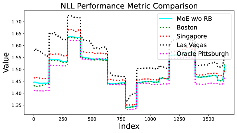
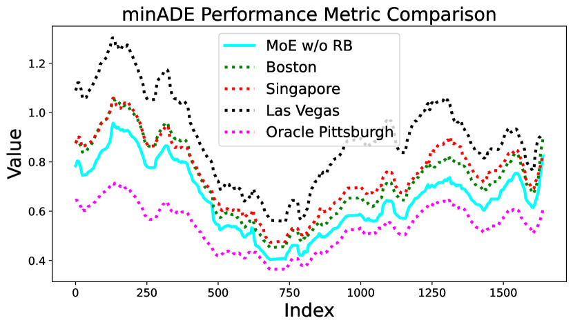
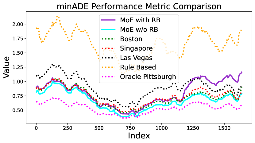
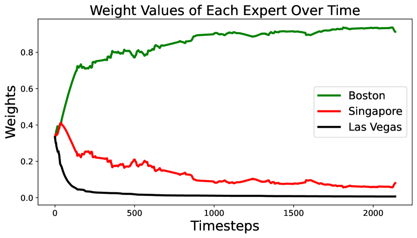
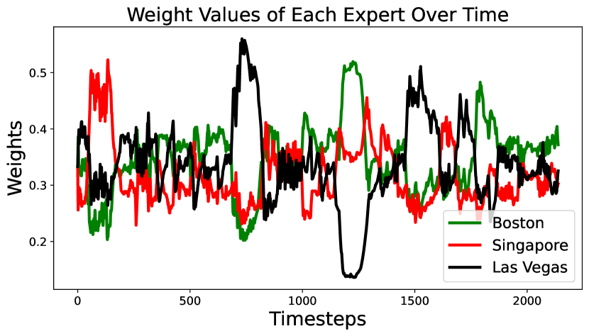
(a) Convex probability loss (5)	(b) Nonconvex minFRDEk loss (10)

Figure 2: Performance of MoE in a stationary distribution shift (from the Pittsburgh environment) using (a) convex loss and (b) nonconvex loss. From top to bottom: NLL performance of the MoE compared with the singular models; minADE performance of the MoE compared with the singular models; evolution of the probability vector. minFDE performance is shown in Appendix -C.

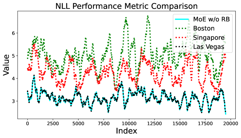
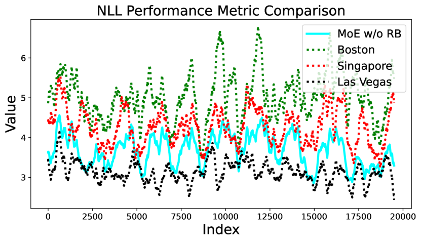
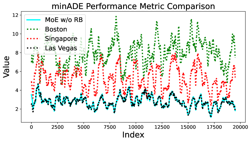
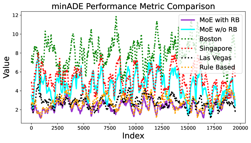
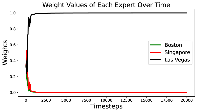
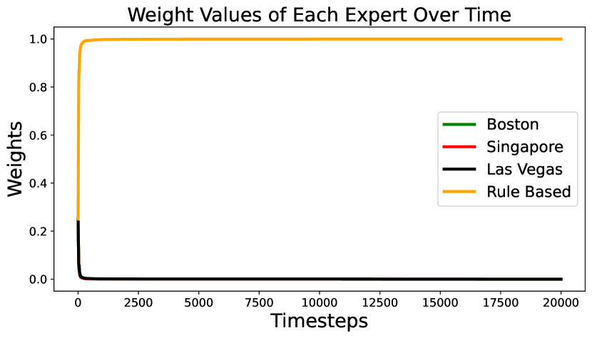
(a) Convex probability loss (5)	(b) Nonconvex minFRDEk loss (10)

Figure 3: Performance of MoE in a stationary distribution shift (from the Lyft dataset) using (a) convex loss and (b) nonconvex loss. From top to bottom: NLL performance of the MoE compared with the singular models; minADE performance of the MoE compared with the singular models; evolution of the probability vector.

Convex Loss. We first evaluate the performance of MoE using the convex probability loss (5). Since the rule-based trajectory predictor does not output covariance in its predictions, we only aggregate the three learned predictors. To simulate distribution shifts, we tested the MoE on the Pittsburgh environment of nuScenes. Fig. 2(a) plots the results. We have the following observations. (i) Looking at Fig. 2(a) bottom, as the theory predicted, the squint algorithm converges to choosing the best expert in hindsight, which is the model pretrained in the Boston split (this intuitively makes sense because Boston is similar to Pittsburgh). (ii) Looking at Fig. 2(a) top and middle, we see the MoE’s performance, in terms of both NLL and minADE, is better than any of the singular models, and is even close to the oracle Pittsburgh model (that is trained on Pittsburgh). Similar observations hold for the minFDE performance and are shown in Appendix -C. We then aggregate the pretrained models and test on the Lyft dataset [21], whose results are shown in Fig. 3(a). We observe that the MoE model quickly converges to choosing the Las Vegas model as the best expert, and the performance of the MoE model closely tracks that of the best expert Las Vegas.

Nonconvex Loss. We then evaluate the MoE’s performance using the nonconvex minFRDE_k loss. In this case, we have two MoEs, one that only aggregates the learned predictors (denoted MoE w/o RB), and the other that aggregates the rule-based predictor in addition (denoted MoE with RB). Fig. 2(b) plots the results of aggregation on the Pittsburgh dataset. We have the following observations. (i) Looking at Fig. 2(b) bottom, we see that, unlike the case of convex loss, the probability vector $\alpha$ does not converge. (ii) Even though the probability vector does not converge, the MoE’s performance is still better than all the other singular models when evaluated using the minADE performance metric (cf. Fig. 2(b) middle). (iii) When evaluated using the NLL performance metric (in which case we only evaluate MoE w/o RB because the rule-based predictor does not output covariance), the MoE’s performance is better than the Las Vegas model and close to the Boston and Singapore model, though slightly worse. This is expected because the minFRDE loss function does not encourage the minimization of the NLL metric. Fig. 3(b) plots the results of aggregation on the Lyft dataset. We observe that since the Lyft dataset is very different from nuScenes, pretrained models on nuScenes perform poorly but the rule-based predictor maintains good performance. In this case, the MoE model quickly converges to choosing the rule-based model as the best expert. We emphasize that the incorporation of the rule-based model into MoE would not have been possible without generalizing the OCO framework to handle the nonconvex and nonsmooth minFRDE_k loss.

IV-B Nonstationary Environment

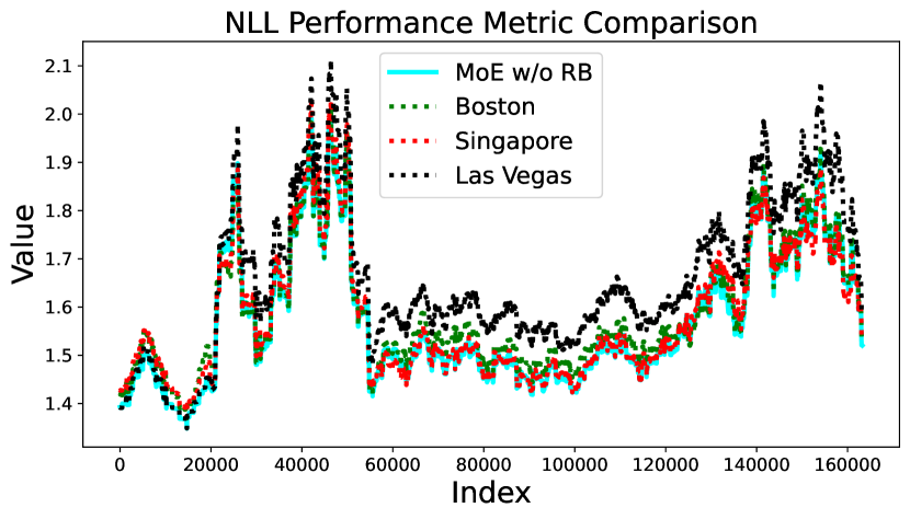
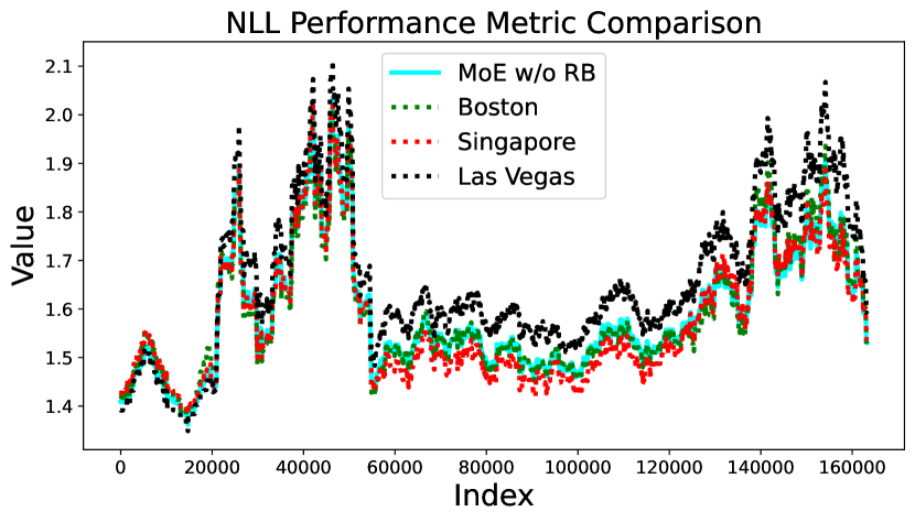
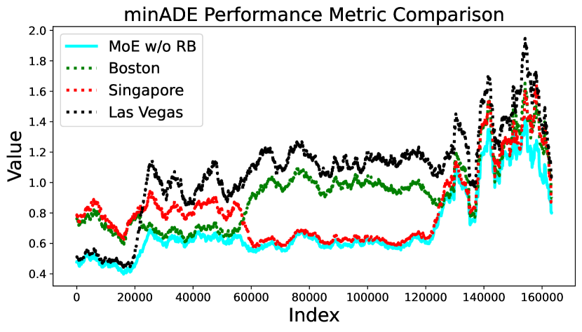
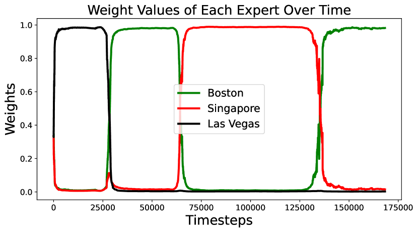
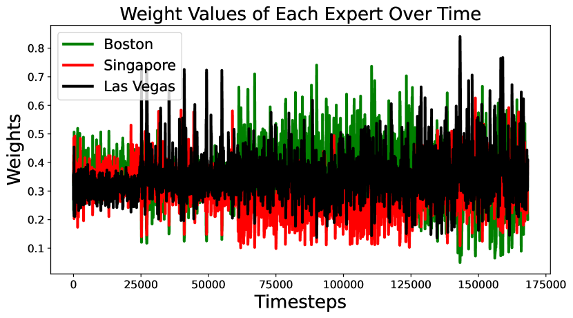
(a) Convex probability loss (5)	(b) Nonconvex minFRDEk loss (10)

Figure 4: Performance of MoE in nonstationary distribution shifts using (a) convex loss and (b) nonconvex loss. From top to bottom: NLL performance of the MoE compared with the singular models; minADE performance of the MoE compared with the singular models; evolution of the probability vector. minFDE performance is shown in Appendix -C.

We then let the distribution shifts happen three times, at roughly timestep 25,000, 60,000, and 130,000 from Las Vegas to Boston to Singapore to Pittsburgh.

Convex Loss. Fig. 4(a) plots the result using the convex probability loss. We observe that (i) the squint algorithm rapidly adapts the probability vector during shifts (Fig. 4(a) bottom). In each distribution shift, the algorithm quickly converges to the best expert within that time window. Notably, the squint algorithm accomplishes this without any prior knowledge of when the distribution shifts occur. (ii) The result of this rapid adaptation is shown in the performance plots (Fig. 4(a) top and middle). The MoE model’s performance tracks the performance of the best expert. Though the performance of each singular model fluctuates, the MoE’s performance is always close to the best singular model.

Nonconvex Loss. When using the nonconvex loss, the probability vector does not converge and it is hard to observe a pattern in the time series of probability vectors (Fig. 4(b) bottom). However, the performance of the MoE model remains robust to distribution shifts, consistently achieving near-optimal performance at all time steps.

V Conclusion

We draw from Online Convex Optimization theory and introduce a light-weight and model-agnostic framework to aggregate multiple trajectory predictors online. Our framework leverages the squint algorithm originally designed for hedging and extends it to the case of nonconvex and nonstationary environments. Results on the nuScenes and the Lyft datasets show that our framework effectively combines multiple singular models to form a stronger mixture model.

Limitation. (i) Aggregating multiple models comes at the cost of running several models online. While this overhead can be mitigated through GPU parallelization, future work should explore using smaller neural networks as individual experts to reduce runtime costs. (ii) Due to the scarcity of data splits, we aggregated only three and four models. Future work should investigate the aggregation of tens or even hundreds of models for trajectory prediction or other applications.

-A Exponentiated Gradient and Comparison with squint

The exponentiated gradient (EG) algorithm [13] is presented in Algorithm 2 (See [47] for a brief introduction).

Input: A prior distribution of the weights $\alpha_{1}$

1 for $t=1,2,\dots,T$ do

2    Compute $\ell_{t}$ as in (5) and define the gradient $\tilde{g}_{t}=\nabla_{\alpha_{t}}(\ell_{t})\in{{\mathbb{R}}^{N}}$

3   Set $G_{t}=\max(\max_{i\in[N]}(|\tilde{g}_{t,i}|),G_{t-1})$ ($\tilde{g}_{t,i}$ denotes the $i$-th element of $\tilde{g}_{t}$)

4   Define the clipped gradient $g_{t}=\frac{(\tilde{g}_{t}/G_{t})+1}{2}\in{{\mathbb{R}}^{N}}$ (element-wise division)

5   Update

$$w_{t+1,i}=\exp\left(-\frac{\sum_{\tau=1}^{t-1}g_{\tau}(i)\sqrt{\ln N}}{\sqrt{t}}\right)$$ (12)

6   Update $\alpha_{t+1}=\frac{w}{\sum_{i=1}^{N}w_{i}}$

Algorithm 2 Exponentiated Gradient

We evaluated both the EG algorithm and squint on the Las Vegas dataset, where we expect the algorithms to converge on choosing the Las Vegas model as the best expert. Fig. 5 shows the evolution of the probability vector $\alpha_{t}$ over time for (a) EG and (b) squint. Notably, squint converges approximately 25 times faster than EG, demonstrating a significant improvement in adaptation speed.

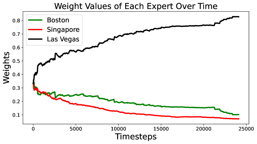
(a) Exponentiated Gradient

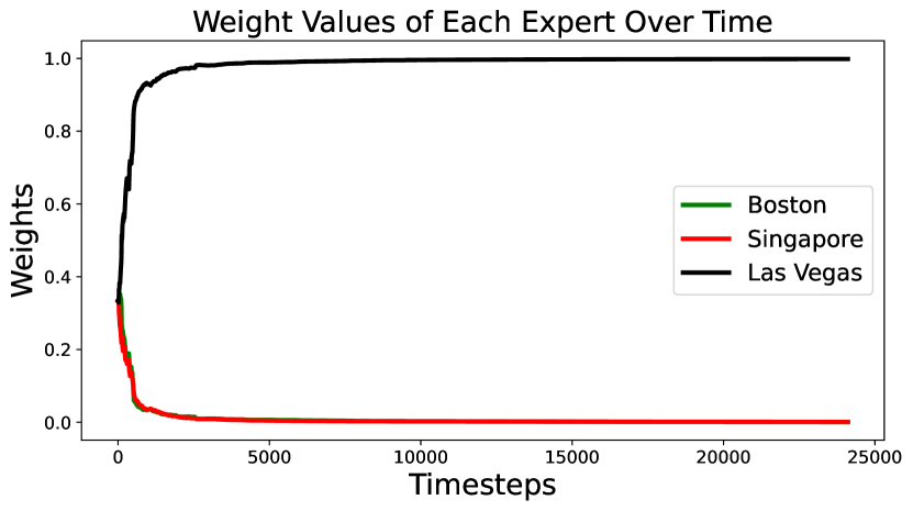
(b) squint

Figure 5: squint vs EG on the Las Vegas dataset.

-B Experimental Details

For the stationary environment, we evaluate our models using the nuplan_mini-pittsburgh dataset from nuScenes. To test performance under nonstationary conditions, we concatenate multiple datasets together in sequence: nuplan_mini-las_vegas, nuplan_val-boston, nuplan_val-singapore, nuplan_val-pittsburgh.

We use $\beta=10$ as the temperature scaling factor in $\mathrm{softmin}$.

We set the discount factor $\lambda=0.9999$ in the nonstationary setup.

We use $k=10$ in choosing the top-$k$ modes.

-C Further Experimental Results

Fig. 6 plots extra results in the stationary setup.

Fig. 7 plots extra results in the nonstationary setup.

At first glance, the behavior shown in Fig. 6 may seem counterintuitive since the probability vector favors the rule-based expert despite its poor performance. However, this preference stems from the rule-based expert’s underlying design: it first predicts the agent’s desired lane and then plans to maintain that position. While this strategy is typically effective, prediction errors jump up drastically when the initial lane choice is incorrect. This is then heavily emphasized by the sliding window averaging we employ, making the rule-based expert’s overall performance appear significantly worse than other experts, even though it performs well in most cases where the lane prediction is accurate.

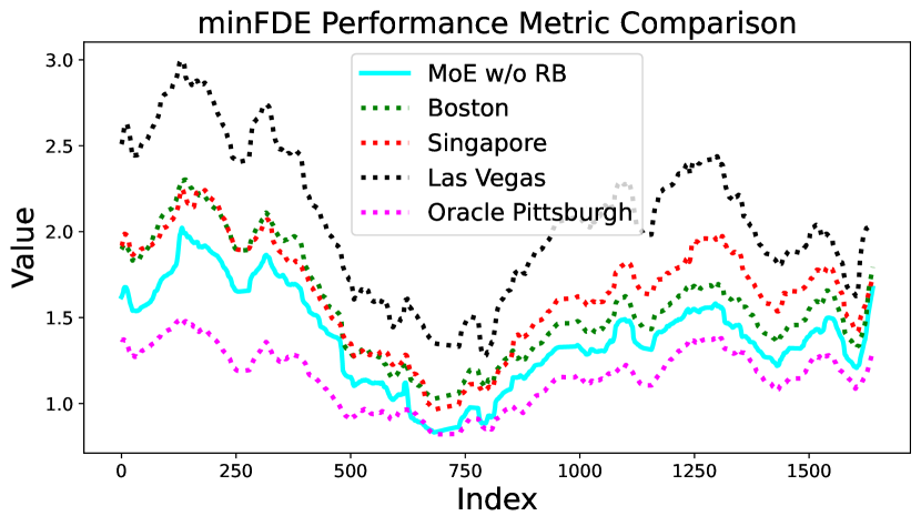
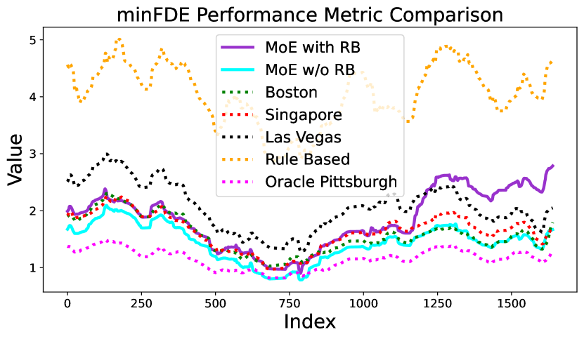
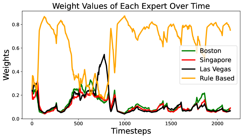
(a) Convex probability loss (5)	(b) Nonconvex minFRDEk loss (10) with RB

Figure 6: More results on the performance of MoE in a stationary setting using (a) probability loss and (b) minFRDE loss. (a) shows the minFDE performance metric. (b) top shows the minFDE performance metric and (b) bottom shows the evolution of the probability vector when aggregating three learned predictors and one rule-based predictor.

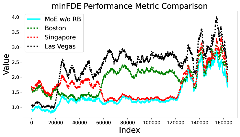
(a) Convex probability loss (5)

(b) Nonconvex minFRDEk loss (10)

Figure 7: minFDE performance metric in a nonstationary setting using (a) convex probability loss and (b) nonconvex minFRDE loss.

-D Generality of the Framework

In this section, we elaborate on Remark 1 and show that our online aggregation framework presented in Section III can handle cases where the pretrained predictors output arbitrary distributions (i.e., not necessarily GMMs), as long as they can be sampled from.

Problem Setup At time $t$, we are given $N$ expert trajectory predictors, where each predictor predicts an arbitrary distribution of trajectories. We assume that this arbitrary distribution can be sampled from, and, in particular, the $i$-th expert generates $M$ trajectory samples

$${\cal T}^{i}_{t}=\{x^{i}_{1,t},x^{i}_{2,t},\dots,x^{i}_{M,t}\},\quad i=1,\dots,N,$$ (13)

where the superscript $i$ denotes the expert index. Similar to Section III, we want to choose a probability vector $\alpha_{t}\in\Delta_{N}$, where each $\alpha_{i,t}$ represents the weight assigned to the $i$-th trajectory predictor.

Loss Function for OCO To evaluate the performance of our MoE, a natural strategy is to compute a suitable loss between the individual trajectory samples ${\cal T}^{i}_{t},i=1,\dots,N$ and the groundtruth trajectory $x_{t}$, and then seek to minimize the weighted sum of the individual losses. Formally, at time $t$, we design the loss function of $\alpha_{t}$ as

$$\ell_{t}(\alpha_{t})=\sum_{i=1}^{N}\alpha_{i,t}\ell_{t}^{i}({\cal T}^{i}_{t},x_{t}),$$ (14)

where the individual loss of each expert, $\ell_{t}^{i}(\cdot)$, is any meaningful loss function that computes the performance of the $i$-th expert. The simplest choice would be

$$\ell^{i}_{t}({\cal T}^{i}_{t},x_{t})=\frac{1}{M}\sum_{j=1}^{M}\|x^{i}_{j,t}-x_{t}\|^{2},$$ (15)

where the mean squared error is computed. Another choice, if the designer is only concerned with the “good” trajectory samples, is to pick the best $k$ samples and compute their mean squared error, i.e.,

$$\ell^{i}_{t}({\cal T}^{i}_{t},x_{t})=\frac{1}{k}\sum_{j=1}^{k}\mathrm{topk}\left\{\|x^{i}_{j,t}-x_{t}\|^{2}\right\}_{j=1}^{M},$$ (16)

where the function $\mathrm{topk}(\cdot)$ selects the $k$ minimum scalars.

squint. A crucial observation is that the loss function $\ell_{t}(\alpha_{t})$ in (14) remains a linear function of $\alpha_{t}$. Therefore, squint presented in Algorithm 1 can still be applied without any modifications.

Mixture of Experts from Importance Sampling. How do we form the Mixture-of-Experts (MoE) model in this case? The answer is to use importance sampling. Specically, the MoE model consists of a new set of $M$ trajectory samples drawn from the mixture of distributions (each generated by one expert), with the mixing weights being $\alpha_{t}$. One way to achieve this is to draw $\lfloor M\alpha_{i,t}\rfloor$ random samples from the $i$-th expert. Intuitively, if the weight of the first expert $\alpha_{1,t}$ decreases to near zero (due to the loss $\ell^{1}_{t}({\cal T}^{1}_{t},x_{t})$ being very large), then the MoE samples will effectively exclude the first expert.

Comparison with GMM. After the discussion above, we see that Online Convex Optimization (OCO) can be applied to the online aggregation of arbitrary distributions, as long as they can be sampled from. Moreover, the algorithm remains unchanged, with the only difference being in the computation of the loss functions. However, we emphasize that a key drawback of the loss function (14) is its reliance on sampling from the distributions, which may require a large number of samples $M$ to ensure fast convergence.

References

- [1] A. Censi, K. Slutsky, T. Wongpiromsarn, D. Yershov, S. Pendleton, J. Fu, and E. Frazzoli, “Liability, ethics, and culture-aware behavior specification using rulebooks,” in 2019 International Conference on Robotics and Automation (ICRA). IEEE, 2019, pp. 8536–8542.
- [2] S. Veer, K. Leung, R. K. Cosner, Y. Chen, P. Karkus, and M. Pavone, “Receding horizon planning with rule hierarchies for autonomous vehicles,” in 2023 IEEE International Conference on Robotics and Automation (ICRA). IEEE, 2023, pp. 1507–1513.
- [3] B. Helou, A. Dusi, A. Collin, N. Mehdipour, Z. Chen, C. Lizarazo, C. Belta, T. Wongpiromsarn, R. D. Tebbens, and O. Beijbom, “The reasonable crowd: Towards evidence-based and interpretable models of driving behavior,” in 2021 IEEE/RSJ International Conference on Intelligent Robots and Systems (IROS). IEEE, 2021, pp. 6708–6715.
- [4] T. Salzmann, B. Ivanovic, P. Chakravarty, and M. Pavone, “Trajectron++: Dynamically-feasible trajectory forecasting with heterogeneous data,” in European Conf. on Computer Vision (ECCV). Springer, 2020, pp. 683–700.
- [5] Y. Chen, B. Ivanovic, and M. Pavone, “Scept: Scene-consistent, policy-based trajectory predictions for planning,” in IEEE Conf. on Computer Vision and Pattern Recognition (CVPR), 2022, pp. 17 103–17 112.
- [6] Y. Yuan, X. Weng, Y. Ou, and K. M. Kitani, “Agentformer: Agent-aware transformers for socio-temporal multi-agent forecasting,” in Proceedings of the IEEE/CVF International Conference on Computer Vision, 2021, pp. 9813–9823.
- [7] R. Bommasani, D. A. Hudson, E. Adeli, R. Altman, S. Arora, S. von Arx, M. S. Bernstein, J. Bohg, A. Bosselut, E. Brunskill et al., “On the opportunities and risks of foundation models,” arXiv preprint arXiv:2108.07258, 2021.
- [8] B. Wang, W. Chen, H. Pei, C. Xie, M. Kang, C. Zhang, C. Xu, Z. Xiong, R. Dutta, R. Schaeffer et al., “Decodingtrust: A comprehensive assessment of trustworthiness in gpt models,” arXiv preprint arXiv:2306.11698, 2023.
- [9] D. M. H. Nguyen, T. N. Pham, N. T. Diep, N. Q. Phan, Q. Pham, V. Tong, B. T. Nguyen, N. H. Le, N. Ho, P. Xie et al., “On the out of distribution robustness of foundation models in medical image segmentation,” arXiv preprint arXiv:2311.11096, 2023.
- [10] H. Liu, W. Xue, Y. Chen, D. Chen, X. Zhao, K. Wang, L. Hou, R. Li, and W. Peng, “A survey on hallucination in large vision-language models,” arXiv preprint arXiv:2402.00253, 2024.
- [11] R. E. Schapire et al., “A brief introduction to boosting,” in Ijcai, vol. 99, no. 999. Citeseer, 1999, pp. 1401–1406.
- [12] R. Meir and G. Rätsch, “An introduction to boosting and leveraging,” in Advanced Lectures on Machine Learning: Machine Learning Summer School 2002 Canberra, Australia, February 11–22, 2002 Revised Lectures. Springer, 2003, pp. 118–183.
- [13] F. Orabona, “A modern introduction to online learning,” arXiv preprint arXiv:1912.13213, 2019.
- [14] Z. Zhang, H. Yang, A. Cutkosky, and I. C. Paschalidis, “Improving adaptive online learning using refined discretization,” in International Conference on Algorithmic Learning Theory. PMLR, 2024, pp. 1208–1233.
- [15] W. M. Koolen and T. van Erven, “Second-order quantile methods for experts and combinatorial games,” 2015.
- [16] A. Cutkosky, “Artificial constraints and lipschitz hints for unconstrained online learning,” arXiv preprint arXiv:1902.09013, 2019.
- [17] A. Grover, E. Wang, A. Zweig, and S. Ermon, “Stochastic optimization of sorting networks via continuous relaxations,” arXiv preprint arXiv:1903.08850, 2019.
- [18] Z. Zhang, D. Bombara, and H. Yang, “Discounted adaptive online learning: Towards better regularization,” in Intl. Conf. on Machine Learning (ICML), 2024.
- [19] H. Caesar, V. Bankiti, A. H. Lang, S. Vora, V. E. Liong, Q. Xu, A. Krishnan, Y. Pan, G. Baldan, and O. Beijbom, “nuscenes: A multimodal dataset for autonomous driving,” in Proceedings of the IEEE/CVF conference on computer vision and pattern recognition, 2020, pp. 11 621–11 631.
- [20] S. Veer, A. Sharma, and M. Pavone, “Multi-predictor fusion: Combining learning-based and rule-based trajectory predictors,” in Conference on Robot Learning (CoRL), 2023.
- [21] J. Houston, G. Zuidhof, L. Bergamini, Y. Ye, L. Chen, A. Jain, S. Omari, V. Iglovikov, and P. Ondruska, “One thousand and one hours: Self-driving motion prediction dataset,” in Conference on Robot Learning. PMLR, 2021, pp. 409–418.
- [22] A. Houenou, P. Bonnifait, V. Cherfaoui, and W. Yao, “Vehicle trajectory prediction based on motion model and maneuver recognition,” in 2013 IEEE/RSJ International Conference on Intelligent Robots and Systems, 2013, pp. 4363–4369.
- [23] A. Alahi, K. Goel, V. Ramanathan, A. Robicquet, L. Fei-Fei, and S. Savarese, “Social lstm: Human trajectory prediction in crowded spaces,” in 2016 IEEE Conference on Computer Vision and Pattern Recognition (CVPR), 2016, pp. 961–971.
- [24] A. Kamenev, L. Wang, O. B. Bohan, I. Kulkarni, B. Kartal, A. Molchanov, S. Birchfield, D. Nistér, and N. Smolyanskiy, “Predictionnet: Real-time joint probabilistic traffic prediction for planning, control, and simulation,” 2022.
- [25] A. Gupta, J. Johnson, L. Fei-Fei, S. Savarese, and A. Alahi, “Social GAN: Socially acceptable trajectories with generative adversarial networks,” in IEEE Conf. on Computer Vision and Pattern Recognition (CVPR), 2018, pp. 2255–2264.
- [26] I. Bae, J. Lee, and H.-G. Jeon, “Can language beat numerical regression? language-based multimodal trajectory prediction,” arXiv preprint arXiv:2403.18447, 2024.
- [27] H. Song, D. Luan, W. Ding, M. Y. Wang, and Q. Chen, “Learning to predict vehicle trajectories with model-based planning,” 2021.
- [28] D. Li, Q. Zhang, Z. Xia, K. Zhang, M. Yi, W. Jin, and D. Zhao, “Planning-inspired hierarchical trajectory prediction for autonomous driving,” 2023.
- [29] X. Li, G. Rosman, I. Gilitschenski, J. DeCastro, C.-I. Vasile, S. Karaman, and D. Rus, “Differentiable logic layer for rule guided trajectory prediction,” in Proceedings of the 2020 Conference on Robot Learning, ser. Proceedings of Machine Learning Research, J. Kober, F. Ramos, and C. Tomlin, Eds., vol. 155. PMLR, 16–18 Nov 2021, pp. 2178–2194. [Online]. Available: https://proceedings.mlr.press/v155/li21b.html
- [30] L. Sun, X. Jia, and A. D. Dragan, “On complementing end-to-end human behavior predictors with planning,” 2021.
- [31] J. Patrikar, S. Veer, A. Sharma, M. Pavone, and S. Scherer, “Rulefuser: Injecting rules in evidential networks for robust out-of-distribution trajectory prediction,” arXiv preprint arXiv:2405.11139, 2024.
- [32] N. Agarwal, B. Bullins, E. Hazan, S. Kakade, and K. Singh, “Online control with adversarial disturbances,” in International Conference on Machine Learning. PMLR, 2019, pp. 111–119.
- [33] E. Hazan and K. Singh, “Introduction to online nonstochastic control,” arXiv preprint arXiv:2211.09619, 2022.
- [34] A. Muppidi, Z. Zhang, and H. Yang, “Fast trac: A parameter-free optimizer for lifelong reinforcement learning,” Advances in Neural Information Processing Systems, vol. 37, pp. 51 169–51 195, 2024.
- [35] I. Gibbs and E. Candes, “Adaptive conformal inference under distribution shift,” Advances in Neural Information Processing Systems, vol. 34, pp. 1660–1672, 2021.
- [36] A. Bhatnagar, H. Wang, C. Xiong, and Y. Bai, “Improved online conformal prediction via strongly adaptive online learning,” in International Conference on Machine Learning. PMLR, 2023, pp. 2337–2363.
- [37] N. Nayakanti, R. Al-Rfou, A. Zhou, K. Goel, K. S. Refaat, and B. Sapp, “Wayformer: Motion forecasting via simple & efficient attention networks,” in 2023 IEEE International Conference on Robotics and Automation (ICRA). IEEE, 2023, pp. 2980–2987.
- [38] S. Shi, L. Jiang, D. Dai, and B. Schiele, “Mtr++: Multi-agent motion prediction with symmetric scene modeling and guided intention querying,” IEEE Transactions on Pattern Analysis and Machine Intelligence, 2024.
- [39] Y. Freund and R. E. Schapire, “A decision-theoretic generalization of on-line learning and an application to boosting,” Journal of Computer and System Sciences, vol. 55, no. 1, pp. 119–139, 1997.
- [40] R. Pascanu, T. Mikolov, and Y. Bengio, “Understanding the exploding gradient problem,” CoRR, abs/1211.5063, vol. 2, no. 417, p. 1, 2012.
- [41] E. Gorbunov, M. Danilova, and A. Gasnikov, “Stochastic optimization with heavy-tailed noise via accelerated gradient clipping,” Advances in Neural Information Processing Systems, vol. 33, pp. 15 042–15 053, 2020.
- [42] J. Zhang, S. P. Karimireddy, A. Veit, S. Kim, S. Reddi, S. Kumar, and S. Sra, “Why are adaptive methods good for attention models?” Advances in Neural Information Processing Systems, vol. 33, pp. 15 383–15 393, 2020.
- [43] R. T. Rockafellar, Convex Analysis. Princeton University Press, 1970.
- [44] S. Prillo and J. M. Eisenschlos, “Softsort: A continuous relaxation for the argsort operator,” 2020.
- [45] H. Caesar, J. Kabzan, K. S. Tan, W. K. Fong, E. Wolff, A. Lang, L. Fletcher, O. Beijbom, and S. Omari, “Nuplan: A closed-loop ml-based planning benchmark for autonomous vehicles,” 2022.
- [46] J. Ngiam, B. Caine, V. Vasudevan, Z. Zhang, H.-T. L. Chiang, J. Ling, R. Roelofs, A. Bewley, C. Liu, A. Venugopal et al., “Scene transformer: A unified architecture for predicting multiple agent trajectories,” arXiv preprint arXiv:2106.08417, 2021.
- [47] University of Washington, “Lecture 10: Exponentiated gradient descent,” 2012, cSE 599S: Special Topics in Theoretical Computer Science, Spring 2012. [Online]. Available: https://courses.cs.washington.edu/courses/cse599s/12sp/scribes/lecture10.pdf