Flexible inference of evolutionary accumulation dynamics using uncertain observational data

Abstract

Understanding and predicting evolutionary accumulation pathways is a key objective in many fields of research, ranging from classical evolutionary biology to diverse applications in medicine. In this context, we are often confronted with the problem that data is sparse and uncertain. To use the available data as best as possible, inference approaches that can handle this uncertainty are required. One way that allows us to use not only cross-sectional data, but also phylogenetic related and longitudinal data is using ‘hypercubic inference’ models. In this article we introduce HyperLAU, a new algorithm for hypercubic inference that makes it possible to use datasets including uncertainties for learning evolutionary pathways. Expanding the flexibility of accumulation modelling, HyperLAU allows us to infer dynamic pathways and interactions between features, even when large sets of particular features are unobserved across the source dataset. We show that HyperLAU is able to highlight the main pathways found by other tools, even when up to 50% of the features in the input data are uncertain.

1 Introduction

Many processes in the natural sciences and especially in biology and medicine can be modelled as the accumulation or loss of binary features [Diaz-Uriarte, 2023, Schill et al., 2024b]. Common examples include evolutionary processes, such as accumulation of mutations in cancer [Schwartz and Schäffer, 2017, Diaz-Uriarte and Vasallo, 2019, Beerenwinkel et al., 2015, Takeshima and Ushijima, 2019, Moen and Johnston, 2023], gene loss in mitochondria [Johnston and Williams, 2016, Maier et al., 2013], mutations in bacteria [Nichol et al., 2015, Tan et al., 2011, Greenbury et al., 2020], and the appearance of other phenotypic characters [Moen and Johnston, 2023, Nichol et al., 2015]. Other examples of accumulation processes include, for example, patients acquiring symptoms in progressing diseases [Dalgıç et al., 2021, Johnston et al., 2019, Schill et al., 2024a].

Understanding and predicting such processes can contribute both to the basic knowledge of the mechanisms involved, and to potential application – for example, in triaging patients [Johnston et al., 2019] and determining optimal treatments [Aga et al., 2024, Renz et al., 2024]. To address this problem many different types of mathematical models for accumulation processes have been derived over the last decades, many of them using discrete binary structures. Among the first models in this context, the Mk (Markov k-state) model [Pagel, 1994, Lewis, 2001] for the evolution of traits across a group of related species were introduced. Recently, [Johnston and Diaz-Uriarte, 2024] demonstrated how the Mk model can be used to infer accumulation processes, including the possibility of reversible transitions.

A large class of models has also been developed, mainly motivated by cancer progression, to infer accumulation pathways from independent, cross-sectional observations. Several of these attempt to construct a graphical structure describing dependencies between events (usually mutations). Such approaches include Oncogenetic Trees (OT) [Desper et al., 1999, Szabo and Boucher, 2002] and the Mutation Order (MO) model [Gao et al., 2022] for modelling the accumulation of mutations in cancer. A generalization of the OT model are the conjunctive Bayesian networks (CBN) [Beerenwinkel et al., 2006, Beerenwinkel et al., 2007] with its specialisations H-CBN [Gerstung et al., 2009] and CT-CBN [Beerenwinkel and Sullivant, 2009]. Here the tree structure is given up and every event can also have more than one ancestor. With the further development of [Montazeri et al., 2016], who introduced new inference methods, it became possible to use CT-CBNs also for large-scale inference. While the CBN models require all ancestor mutations before further progression, in the disjunctive Bayesian networks [Nicol et al., 2021] this assumption is relaxed to the extend that only one parent needs to be present that a mutation can happen. [Youn and Simon, 2012] developed a model that estimates the probability distribution for the order in which the mutations occur by maximizing a log-likelihood function. Here the input data has not to be binary, but can contain higher numbers when there is more than one mutation in a gene.

A separate class of these approaches consider probabilistic progression through a state space, with dependencies between events now changing transition probabilities rather than reflecting deterministic requirements. [Hjelm et al., 2006] learns the pairwise dependencies between chromosomal aberrations in cancer, using a Markov network on the state space of all possible subsets of the considered events, with dependencies restricted to being pairwise and amplifying. HyperTraPS [Johnston and Williams, 2016, Greenbury et al., 2020] and Mutual Hazard Networks (MHN) [Schill et al., 2020, Rupp et al., 2024, Schill et al., 2024a] are two more recent models for evolutionary accumulation. Both model pairwise interactions between events and use a reduced number of parameters by inferring a base rate for every mutation and additionally the pairwise interaction parameters. The MHN way to parameterize the transition probabilities was also the basis for several further developments by [Gotovos et al., 2021, Chen, 2023, Luo et al., 2023]. HyperTraPS-CT, a new development introducing continuous, uncertain timings and the ability to handle phylogenetic and cross-sectional data [Aga et al., 2024], and HyperHMM [Moen and Johnston, 2023] allows arbitrarily complex dependencies between the different mutations, by estimating every transition probability directly. An overview over the recent methods for modelling accumulation and loss of features is given in [Diaz-Uriarte, 2023] and [Schill et al., 2024b].

In several scientific and medical contexts, data on accumulation processes often includes uncertainties and unknown states. The extent to which existing models can handle this uncertainty is typically limited. In most of the named models, there are only general correction mechanisms or error rates included, which can account for some noise. MO [Gao et al., 2022] explicitly allows missing or ambiguous information for specific features, but is subject to the infinite-sites assumption (every event occurs at most once, prohibiting parallel evolution), which is not appropriate in several scientific contexts. HyperTraPS-CT [Aga et al., 2024] does not have this assumption, but represents data as a set of ancestor-descendant states and can only naturally deal with uncertainties in the descendant states, not in the ancestral ones. So far the only model that can fulfill all these requirements is the Mk-model [Johnston and Diaz-Uriarte, 2024] which, however, is limited to very few features due to the high computational runtime.

Here, we introduce HyperLAU (hypercubic transition paths with linear algebra for uncertainty), an approach for accumulation modelling that has no underlying infinite site assumption but can deal with longitudinal input data, including specified uncertainties in ancestor and descendant states. On the same time, it can handle input data with more features than the Mk-model in a smaller amount of time. Taking up the idea of an hypercubic transition graph and the pairwise MHN parameterization, but maintaining the option of longitudinal data as input, we developed an approach where precise positions of uncertainty can be specified in both the ancestor and descendant strings. In the center of the algorithm are simple matrix-vector multiplications, as known from linear algebra, which makes the approach intuitive and easy understandable (see Figure 1). Borrowing the idea for the option to model different orders of dependencies from [Greenbury et al., 2020], we additionally keep this flexibility, what is a further advantage of our model. We will particularly motivate the approach in the context of anti-microbial resistance (AMR) evolution – the evolution of pathogens to different drugs. AMR is one of the top threats to human health worldwide, with 4.95 million deaths associated with AMR in 2019 [Murray et al., 2022]. Data on bacterial drug resistance is often either inferred from genome information (leading to uncertainty) or measured using laborious experiments (often leading to incompleteness). The ability to handle incomplete, phylogenetically-related data is therefore a substantial advantage to accumulation models in this context.

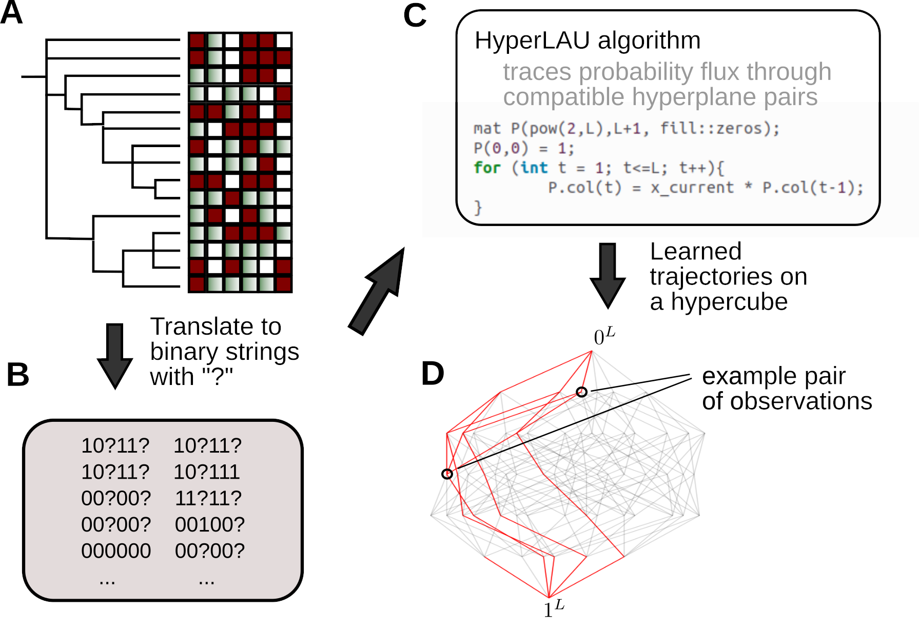
Figure 1: HyperLAU workflow. Learning evolutionary trajectories on a hypercube, based on data that contains uncertainties. (A) Dataset (structure can be cross-sectional or longitudinal) that contains information about the presence (red/dark) or absence (green/gradient) of certain features. White boxes indicate missing/uncertain information. (B) Translation of the data into binary barcodes, 1 = presence of the feature, 0 = absence. The uncertain positions are represented by a ‘?’. (C) The dataset in the form of barcode pairs is given to the HyperLAU algorithm, which consists of the optimization of a likelihood function, whose calculation is based on linear algebra. (D) The HyperLAU algorithm learns the evolutionary pathways and outputs the transition probabilities and fluxes, which can be used to make predictions.

2 Materials and methods

Hypercubic transition paths with Linear Algebra for Uncertainty. We consider a state space $S$ that is the set of all binary strings of length $L$, where $L$ is the number of features in our system. Each binary string describes a state by the presence (1) or absence (0) of each of these $L$ features. A transition from state $s_{i}$ to $s_{j}$ is allowed if the binary string $s_{j}$ differs from $s_{i}$ by the presence of exactly one ‘1’: that is, only transitions that involve the acquisition of one feataure are allowed. The resulting structure is a directed acyclic graph which we call a hypercubic transition graph. The HyperLAU algorithm can be used to learn the transition probabilities $a_{i,j}=\{X_{t}=s_{i}|X_{t-1}=s_{j}\}$ of a discrete Markov process $X_{t}$ on such a hypercubic transition graph.

The likelihood calculation finds the probability that a random walk that runs from the $000...$ state to the $111...$ state and emits exactly two signals compatible with the ancestral and descendant observations in a datapoint. Beginning with an initial guess of a transition matrix, we then optimize the likelihood.

The dataset we use consists of two binary strings for each data point, one ancestor and one descendant state. This way it is possible to describe an evolutionary development of one sample, either measured at two different time points (longitudinal data) or if they are ancestor and descendant. Even cross-sectional data can be used, by setting all positions of all ancestor strings to zero. This reflects the general assumption that every modelled trajectory originally started at the zero-state where no features are obtained. The strength of HyperLAU is thereby, that the strings in the data set can contain uncertain positions, which are indicated by a ‘?’ instead of a 0 or a 1, and describe a lack of knowledge. These uncertainty markers can appear in any number and in both the ancestor and the descendant state and are considered in the likelihood calculation.

HyperLAU allows for inference of the transition parameters under different models for interaction or independence between features involved. The user can choose what level of interactions or influences between the different features they want to allow. This is done by an input parameter model$\in\{F,1,2,3,4\}.$ For model $=F$, arbitrary interactions between all features are allowed. In this case, we learn a transition parameter for every allowed state-to-state transition by itself. We consider the whole transition matrix directly as the object we change in order to optimize the likelihood. For the four other models, state-state transition probabilities are functions of the changing feature and a set of contributions from acquired features, as also used in [Aga et al., 2024]. This means our parameter set consists of a base rate with which every feature occurs, and for model$\in\{2,3,4\}$ additional parameters that reflect the influence that the existence of a set of features can have on the rate with which another feature is obtained. In model = $1$, there is only the base rate and it does not matter what other features are already obtained. The other three models allow accordingly interactions of order two, three or four. In these models, influences between either single respectively pairs or triplets of already acquired features can increase or decrease the probability for other features to occur. During the optimization procedure we make changes only on this parameter set. The transition matrix, which still is used in the calculation of the likelihood, can easily be created from this parameter set.

The core piece of the new method that is presented here, is the calculation of the log-likelihood of seeing the input data for a given transition or rate matrix (see Algorithm 1). This involves the dealing with concrete specified uncertainties in form of uncertainty markers in descendant and ancestor state in the input data and, to the best of our knowledge, is not implemented in any existent method so far.

Algorithm 1 Pseudocode of the calculation of the likelihood with the HyperLAU method.

Input: Vectors with ancestor and descendant states of the data set and the corresponding frequency, length of the strings $L$, transition matrix $A$

Output: log-likelihood of seeing the input data given the transition matrix

1:Set $P_{.,t}=(1,0,...,0)$ (vector of length $2^{L}$, indicates probability distribution at $t=0$)

2:for  $t$ in $1:L$ do

3:  $P_{.,t}=A\cdot P_{.,t-1}$

4:end for

5:for every point in the data set do

6:  vector (length $2^{L}$) $c^{a}$ = binary entries, indicate compatible states for the ancestor

7:  vector (length $2^{L}$) $c^{d}$ = binary entries, indicate compatible states for the descendant

8:  for $t$ in $0:L$ do

9:   $P_{.,0}^{\text{comp}}=c^{a}\star P_{.,t}$ with $\star$ entry-wise multiplication

10:   if sum($P_{.,0}^{\text{comp}}$) $\neq 0$ then

11:     Initialize $Q$ = null-matrix of dimension $2^{L}\times L$

12:     $Q_{.,t}$ = $P_{.,0}^{\text{comp}}$

13:     for $s$ in $t+1:L$ do

14:      $Q_{.,s}$ = $A\cdot Q_{.,s-1}$

15:     end for

16:     for $s$ in $0:L$ do

17:      $Q_{.,s}^{\text{comp}}=c^{d}\star Q_{.,s}$

18:      if sum($Q_{.,s}^{\text{comp}}$) $\neq 0$ then

19:        store sum($Q_{.,s}^{\text{comp}}$)

20:      end if

21:     end for

22:   end if

23:  end for

24:  $lh=$ sum of all stored sum($Q_{.,s}^{\text{comp}}$) multiplied with normalization factor

25:  multiply $lh$ with the corresponding frequency of the data point

26:  take the logarithm for getting the log-likelihood and store this

27:end for

28:Sum over log-likelihoods for all data-points

To take the uncertainty markers that can occur in the dataset into account, we have to consider all nodes in the hypercube that are compatible with the observations:

Definition 2.1.

A node $i$ in the hypercube is compatible with an observation $k^{a}$ (ancestor) or $k^{d}$ (descendant) if and only if all positions in the string that are not represented by a uncertainty marker are equal.

For every observation $k^{i},\ i\in\{a,d\}$, in our dataset the information of compatibility is stored in a vector $c^{a}$ for the ancestor (a) string and a vector $c^{d}$ for the descendant (d) string, where we set $c^{i}_{h}=1$ if node $h$ is compatible with $k^{i}$ and 0 otherwise.
Because we assume that every trajectory starts at $0^{L}$ and in every evolutionary step exactly one new feature is obtained until we end up at $1^{L}$, we need $L+1$ steps to simulate a whole pathway. For a given transition matrix $A$ of the hypercube, we can compute a vector $P_{.,t}$ for every evolutionary step $t=0,...,L$, where $L$ is the length of the strings, i.e. the number of considered features. $P_{i,t}$ is then the probability of a trajectory being in evolutionary step $t$ at node $i$, where $i$ is the natural number that corresponds to the binary string. That means, every $P_{.,t}$ gives a probability distribution of occupancy for the different nodes of the hypercube at step $t$.
Set $P_{.,0}=[1,0,0,...]$. This reflects our assumption that every trajectory has to start in the state, where none of the features have yet been achieved. Then

$$P_{.,t}=A\cdot P_{.,t-1}=A^{t}\cdot P_{.,0}.$$ (1)

We can now go step-wise through the columns of the matrix $P=(P_{.,t})_{0\leq t\leq L}$, i.e. the evolutionary steps, and determine the likelihood assuming the ancestor data has its origin in this step. To keep only the information about the probability of being in a state that fits our data, we multiply $P_{.,t}$ entry-wise with $c^{a}$. For every $c^{a}\star P_{.,t}$ where there is at least one entry that is bigger than zero, we assume the ancestor can originate from step $t$ and continue by applying the same matrix-vector approach to get vectors $Q_{.,s}^{t,a},\ t\leq s\leq L$ containing the probability distribution for being in a certain node of the hypercube at step $s$ given that the trajectory reached already the ancestor state in step $t$ before. For $s=t$, $Q_{.,s}^{t,a}$ is set to the vector that results when multiplying $P_{.,t}$ entry-wise with $c^{a}$:

$$Q_{.,s}^{t,a}=c^{a}\star P_{.,t}\text{ for }s=t.$$

From here we continue just by multiplying with the transition matrix in the same way as in (1):

$$Q_{.,s+1}^{t,a}=A\cdot Q_{.,s}^{t,a}\quad\text{ for }s={t,...,L}.$$

Then we have to multiply every $Q_{.,s}^{t,a}$ this time with $c^{d}$ so that we end up with the sum of the probabilities also compatible with the descendant state of the data point. This is exactly the probability that a trajectory first goes through a node that is compatible with the ancestor state of the data set, and afterwards through a node that is compatible with the descendant state. We specifically allow the ancestor and the descendant state to be the same one.
Summarized, the likelihood function of seeing a data point can be described by the following formula:

$$\mathcal{L}((k^{a},k^{d})|A)=\frac{2}{(L+1)(L+2)}\cdot\sum_{t=0}^{L}\sum_{s=t}^{L}c^{d}\cdot Q_{.,s}^{t,a}$$ (2)

with

$$Q_{.,s}^{t,a}=A^{s-t}\cdot\left(c^{a}\star P_{.,t}\right).$$

Here $\star$ describes the component-wise multiplication of two vectors and the factor $2/(L+1)(L+2)$ is the normalization constant reflecting the $(L+1)(L+2)/2$ possible combinations of nodes on the hypercube at which ancestor and descendant can be sampled. Calculating Equation (2) for every entry in our data-set, take the logarithm and summing up the obtained log-likelihoods, we get an overall logarithmic likelihood of obtaining the data in the dataset, given the transition matrix. This is also the function that needs to be optimized by adapting the transition or rate matrix.

Optimization and convergence. The optimization process follows a simulated annealing process where in every loop the entries of the transition matrix, or in the reduced case the rate matrix, are changed a small amount. The reason why we preferred simulated annealing over a gradient based approach is its ability to escape local optima and has a good chance to find the global optimum. This is especially important because we have no prior knowledge about the shape of the optimization landscape. The initial temperature is set to 1 and decreased in every loop by dividing by a certain factor, which can be specified as an input parameter. For all results here presented, the temperature was divided by 1.001 in every step. As soon as the temperature falls below a threshold of $10^{-6}$, the iterations and with that the optimization process are stopped. This choice of parameter values gave us a sufficient level of convergence for the datasets we considered (for the progression trajectories of the likelihood see SI). All results of the tuberculosis data are obtained under model $F$.
With each iteration, every parameter is adjusted individually by a random number from the uniform distribution between -0.025 and 0.025. If this leads to a negative value, the parameter is set to zero. The new parameter matrix is accepted over the current one, if the corresponding log-likelihood is bigger than the one before, or if

$$\exp\left(\frac{-(l_{\text{old}}-l_{\text{new}})}{T}\right)>U(0,1),$$

where $l_{\text{old}}$ and $l_{\text{new}}$ are the two log-likelihoods, and $T$ the current temperature.

Bootstrapping. For determining the uncertainty of our inference results we implemented a bootstrap option on the input data. The number of bootstrap resamples can be specified via an input parameter in the command line. All reported CVs in this article are based on 10 bootstrap resamples.

Initial guess of the transition and the rate matrix. As initial guess of the transition matrix for model $F$, we implemented the matrix that represents a uniform distribution of edge weights among all possible nodes that can be directly achieved from the current state.
For models 1-4 we have to infer the parameters contained in a rate matrix setting only the base rates to one and all rates describing influences by sets of already obtained features to zero. Different than in the case of the transition matrix, here are all entries part of the optimization process and can be changed during the Simulated Annealing.
This initial guesses are a natural choice when there are no prior information or assumptions available. However, it is also possible to implement another initial guess, if necessary.

Manipulation of the datasets to artificially insert uncertainty. To establish that our model is able to predict the most likely evolutionary pathways even with uncertain states in the data, we created some test datasets by inserting random uncertainty markers in the original ones. For the toy-example case, we included the uncertainty feature-wise. For the tuberculosis dataset, we spread them uniformly over all positions. For doing so, for each relevant position in every string a random number was drawn from the uniform distribution between zero and one. If the random number was smaller than a specified threshold, the corresponding position in the dataset was changed to a ‘?’, if not, the original binary entry was kept. This procedure was done with thresholds 0.4 for the toy-example and 0.5 for the tuberculosis data. Doing so we get versions of the toy-example dataset with around 40% uncertainty markers in every feature each, as well as a version of the tuberculosis data with uncertainty markers in around 50% of all positions.

Implementation. The code is implemented in C++ and is freely available on Github: https://github.com/JessicaRenz/HyperLAU. The Armadillo library for linear algebra and scientific computing [Sanderson and Curtin, 2016, Sanderson and Curtin, 2019] is used in this code. Additionally there are also R scripts for creating the visualisations of the output, string manipulation and tree processing, which use the libraries ggplot2 [Wickham, 2016], stringr [Wickham, 2023], ggraph [Pedersen, 2024], ggpubr [Kassambara, 2023], igraph [Csardi and Nepusz, 2006, Csárdi et al., 2024] and dplyr [Wickham et al., 2023].

3 Results

3.1 HyperLAU on toy examples

First we demonstrate the effect of our algorithm on illustrative synthetic examples, which contain only a small number of features and a few data points each, so that it is easier to comprehend the obtained results (see concrete calculations in SI).
The first toy example is specified by the longitudinal dataset containing the following three entries: 0?0 - ?00, 10? - 1?0 and 11? - ?11. When considering only three features, there can be no interactions of higher dimension than two, so it is sufficient to consider the models $F$, 1 and 2. The results given by the different models are illustrated in Figure 2 A.

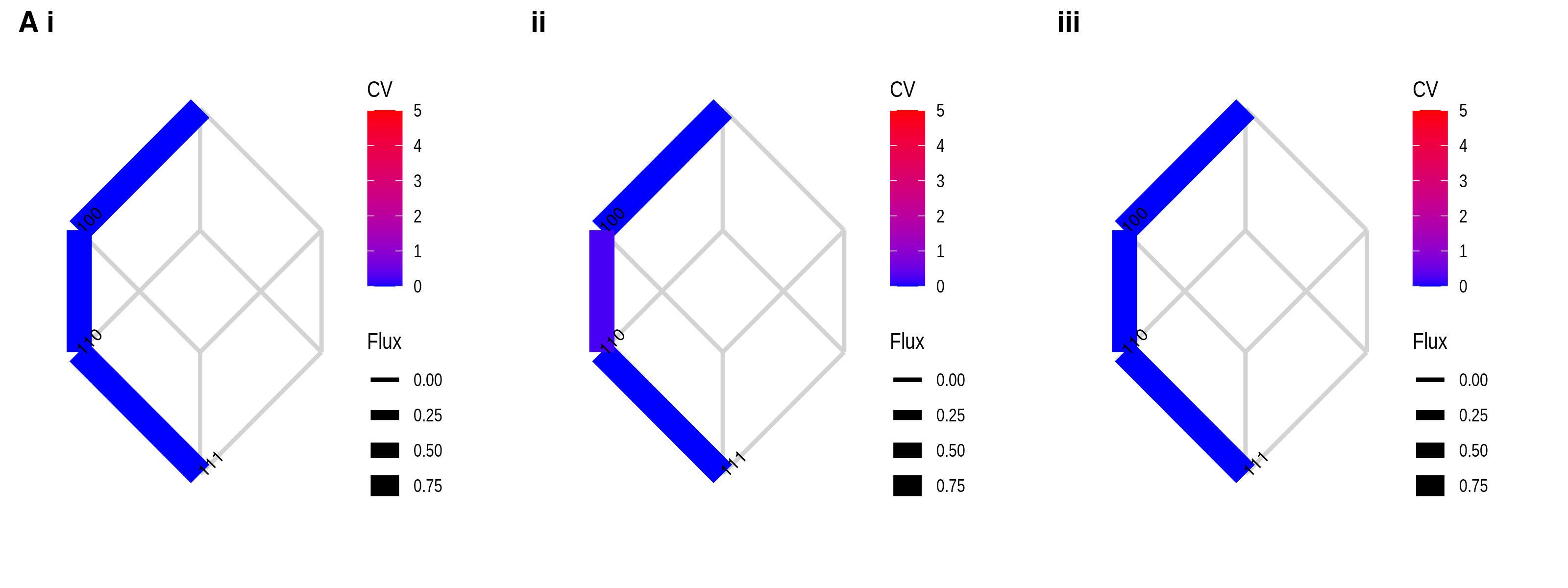
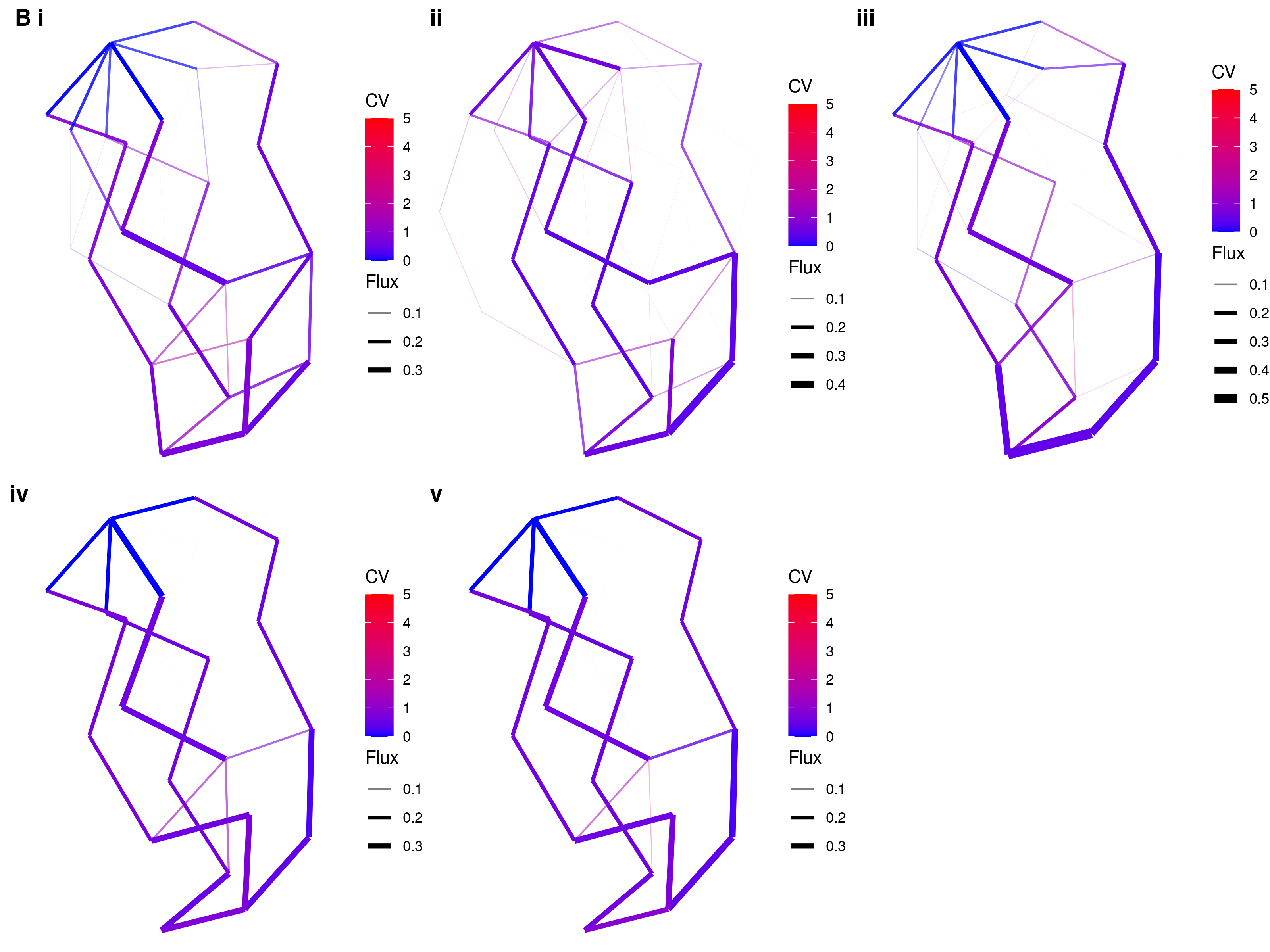
Figure 2: Visualization of the learned fluxes by HyperLAU based on some toy examples. The thickness of the edges represents the strength of the flux. The coefficient of variation (CV) is illustrated by the colour. A: Toy dataset including the data-points 0?0 - ?00, 10? - 1?0 and 11? - ?11, under model $F$ (A i), model 1 (A ii) and model 2 (A iii). The coloured edges correspond to a flux $\geq 0.05$. B: Artificially generated data, where pairs of features influence the occurrence of others (as used in [Aga et al., 2024]), learned (B i) under model $F$, (B ii) with HyperTraPS-CT [Aga et al., 2024], (B iii) under model $F$ but with randomly inserted ‘?’ at about 40% in all strings at feature 1, (B iv) under model 2, (B v) under model 2, but with randomly inserted ‘?’ at about 40% in all strings at feature 3.

To indicate the pairings compatible with the input data, we have to take into account that every ‘?’ could either be a zero or a one. From the first data point, we therefore get the compatible options 000 - 000 and 000 - 100. The other combinations, having 010 in the ancestor state, are not possible, because we assume the attainment of a feature to be irreversible, and the second position in the descendant is clearly marked by a zero. Following the same logic, the second sample gives us either 100 - 100 or 100 - 110, and the last one 110 - 111 or 111 - 111. The combination in which ancestor and descendant are represented by the same string, can’t tell us much about the further progress from the corresponding state. That restricts us to the set of 000 - 100, 100 - 110 and 110 - 111, what depicts the clear path 000 - 100 - 110 - 111. Looking at Figure 2 A, this is predicted by all three models.

The other toy example we present here, is already used to demonstrate the continuous-time version of HyperTraPS [Aga et al., 2024]. The data have its origin in a process, where pairs of already obtained features influence the further evolutionary trajectory in a non-additive way beyond the pairwise interaction picture of MHN. In Figure 2B, we demonstrate that the main tendency of the most likely pathways learned under the full model $F$ allowing arbitrary interactions fit the ones that are learned by HyperTraPS-CT in [Aga et al., 2024] (see Figure 2 B i - ii).

Also, after randomly replacing around 40% of the zeroes and ones representing feature 1 by uncertainty markers, the edges having a high flux are almost the same (Figure 2B iii). Model 2, which only takes into account the influence of existing individual factors, is not able to capture the same full structure (Figure 2B iv). Here we see again, that it can be necessary to allow higher-order interactions to get a better picture of the dynamics that are going one. But also under model 2 the inclusion of around 40% uncertainty in, for example, feature 3 (Figure 2B v) leads to a result that is extremely close to the results of the original data. This also holds for datasets including uncertainty in some of the other features (see SI) and demonstrates that HyperLAU can catch the underlying dynamics, even when up to 40% of the information about one feature is missing. This scenario is common, for example, when you merge datasets from several sources with a different set of features reported.

3.2 HyperLAU on tuberculosis drug resistance data with artificially introduced uncertainties

Additionally to the toy examples, we also want to demonstrate the power of HyperLAU on a real data set of multidrug-resistance data in tuberculosis. The data set we use consists of the binary indication of susceptibility or resistance to 10 drugs for each of 295 isolates and has previously been used to test several other accumulation models [Moen and Johnston, 2023, Greenbury et al., 2020]. It is originally published in [Casali et al., 2014]. We used the same ancestral reconstruction of the phenotypic resistance features as [Moen and Johnston, 2023]. This dataset only contains samples with no uncertainties, every feature in every sample can be clearly represented as a zero or a one. To test HyperLAU’s ability to reproduce inferences in the face of uncertain data, we artificially introduced uncertainties in this dataset, by exchanging every character in the original dataset with a possibility of 50% with a ‘?’, both for the ancestor and the descendant state. The considered features represent resistances against the first-line drugs 1, isoniazid (INH); 2, rifamycin (RIF); 3, pyrazinamide (PZA); 4, ethambutol (EMB) and 5, streptomycin (STR), as well as the second-line drugs 6, amikacin (AMI); 7, capreomycin (CAP); 8, maxifloxacin (MAX); 9, ofloxacin (OFL) and 10, prothionamide (PRO). Training HyperLAU on both datasets, we can compare the learned results (see Figure 3).

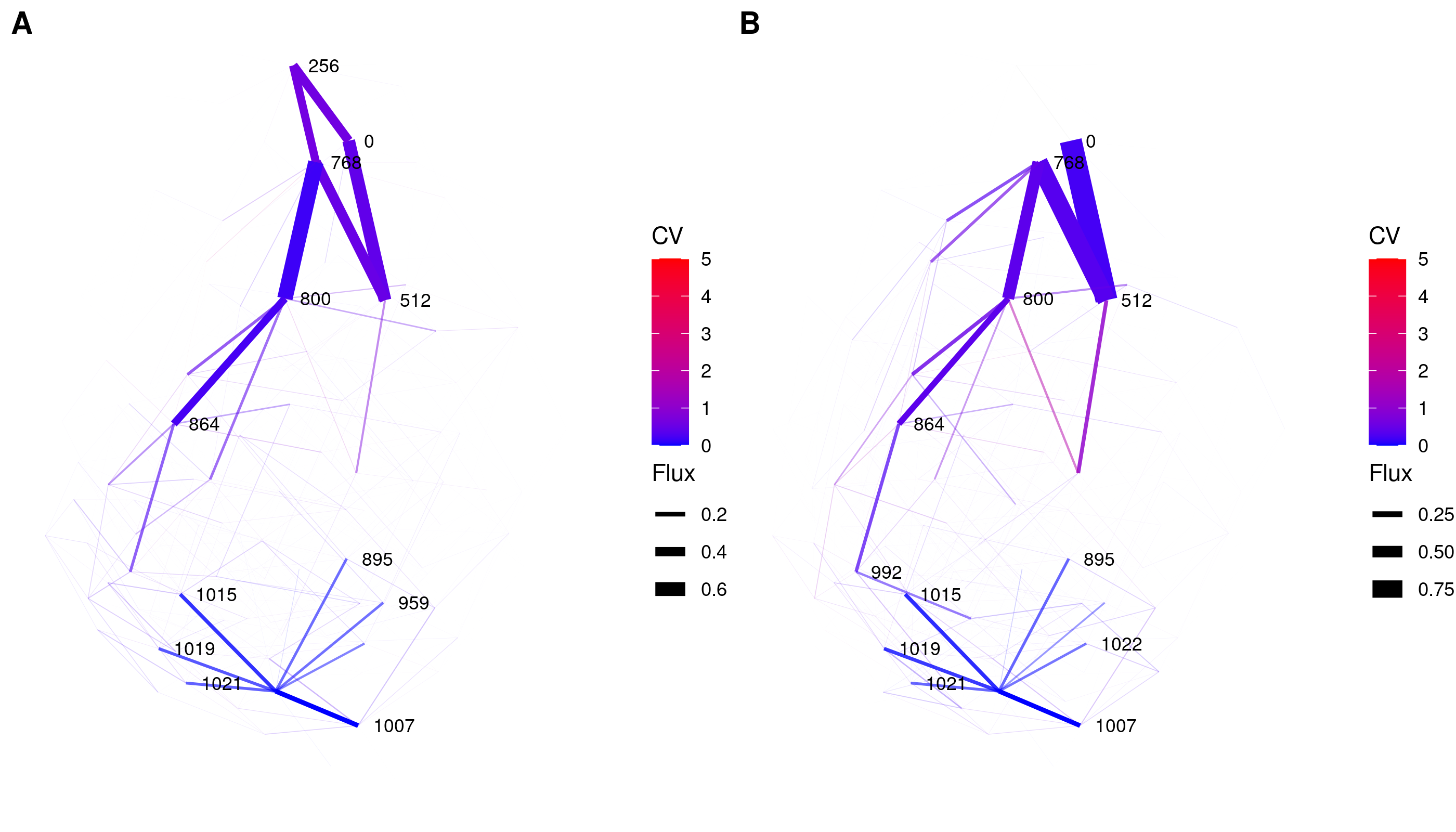
Figure 3: Visualisation of the fluxes learned by HyperLAU based on the tuberculosis data set [Casali et al., 2014]. The thickness of the edges represents the strength of the flux. The coefficient of variation (CV) is illustrated by the colour. A: Original dataset with no uncertainties was used (all samples with missing information were excluded). B: dataset used in A, but every position of the original dataset was replaced by a ‘?’ with probability 0.5. The nodes with the highest outgoing fluxes are labelled with the integer representing the corresponding string in binary notation: 256 = 0100000000, 512 = 10000000000, 768 = 1100000000, 800 = 1100100000, 864 = 1101100000, 992 = 1111100000,…

One can see that even with around 50% uncertain positions in the data, most among the edges with the highest predicted flux for the original data set, are still identified as such by HyperLAU. In the original dataset there is a clear indication that resistance to either INH or RIF is obtained first, although the order seems not unambiguously clear. Afterwards, the resistances against STR, EMB and PZA are acquired, before the further course becomes a bit more fanned out and seems to split into several competitive strains. These results match the results HyperHMM predicted on the same dataset [Moen and Johnston, 2023].
Considering the results of the data with inserted uncertainty, the dynamic in the beginning of obtaining resistance first against INH, then against RIF, STR, EMB and PZA is still very clear. However, in this case the version with INH before RIF is clearly favored. It is also visible that several other edges have a higher flux as before, although with a higher CV. This blurring is to be expected when having more uncertainty.
Of course, when interpreting these results, one has to keep in mind, that the ancestor and descendant relationships of the dataset result from a phylogenetic reconstruction. Introducing random uncertainty markers at each position in the dataset individually can lead to the situation, that two strings representing the same organism in reality, look differently in the end. Also the trajectory for every datapoint is assumed to start at the $0^{L}$ state and reach the considered ancestor state independent of all other datapoints, what is typically not the case for phylogenetically linked data. Nevertheless, for the purpose of showing that HyperLAU is able to capture the most likely and outstanding pathways of a real-world data set, even when up to 50% of the position in the input-data are uncertain this approach is sufficient.

4 Discussion

We introduced HyperLAU as a new tool to learn and model accumulation processes based on binary data which is able to deal with precisely specified uncertainties in input data that consists of an ancestor and a descendant state. An additional advantage of HyperLAU is, that there can be arbitrary interactions between different features taken into account, while there also is the option to reduce the parameter set and follow an approach as used for Mutual Hazard Networks or HyperTraPS. Our different case studies have shown that, given a dataset without any uncertainties, our results align with those of other models, and point out the power to use data without the need to exclude samples due to knowledge gaps.
The HyperLAU algorithm assumes the different data points in the input data to be independent of each other, what needs not to be true for all datasets. This should be kept in mind, and if necessary, previous preparations of the dataset should be done, to account for that. An important situation in which the here used independence assumption does not hold is when considering phylogenetically linked data. When treating all the pairwise ancestor - descendant pairs occurring in a phylogeny as datapoints, it would be necessary to ensure that the interpretation of the uncertainty markers among all strings that represent one and the same position in the phylogeny are consistent. For the moment, HyperLAU is not able to provide this, further work has to be done. Nevertheless, we believe that the possibility to handle uncertainties in ancestor and descendant of pairs in HyperLAU is the first step in this direction.
The Simulated Annealing process includes some random choices of changes in the parameters, so that it could be a valuable procedure to evaluate the results for different random seeds. Furthermore, we consider a setup, where all achieved features are irreversible, what is a simplification that does not necessarily hold true in the actual underlying biological process. Especially when considering antibiotic resistance, the loss of resistance genes that are located on a plasmid is an event that takes place in reasonable frequency. For implementing this option of reversibility, further work is needed, but we think that our linear algebra approach could also be a reasonable starting point for that, for example by allowing also upper-diagonal entries in the transition matrix to be positive.
A disadvantage compared to other models might be the longer run time when considering a larger amount of features. Additionally to the up-scaling due to matrix-vector multiplications with bigger matrices, the run-time also varies with the amount of uncertainty markers in the input-data. With more uncertainty, considerably more possible pathways have to be taken into account to calculate the likelihood. A possible way to address this problem could be the usage of another, more efficient optimization method, or the implementation of a tensor format as in [Schill et al., 2024b].
Compared to HyperTraPS-CT and MHN, which work in a continuous-time setup, HyperLAU is not able to take time as such a factor into account. The temporal order here is represented by evolutionary steps that occur after each other. It is, however, not possible to make statements about the real-life time-scale, in which the evolutionary process takes place. As shown by a case study in [Aga et al., 2024], modelling of such an accumulation process in continuous time instead of discrete time-steps, can lead to different results, when considering less-frequent features that have a fast capture time. Embedding this approach in a continuous-time framework would be an important next step, which further combines the advantages of the different approaches. For now, our hope is, that the here described method is a useful contribution, which allows us to learn accumulation processes on a broader data basis without a prior selection regarding completeness.

Supplementary Information

Calculation of the likelihood for the first toy example in subsection 3.1

This illustrative dataset consists of the following data points:

1. 0?0 ?00

2. 10? 1?0

3. 11? ?11

We can now calculate for every of these three data points the corresponding vectors $c^{a}$ and $c^{d}$ that indicate the compatible states in the hypercube:

1. $c^{a}=(1,0,1,0,0,0,0,0),\quad c^{d}=(1,0,0,0,1,0,0,0)$

2. $c^{a}=(0,0,0,0,1,1,0,0),\quad c^{d}=(0,0,0,0,1,0,1,0)$

3. $c^{a}=(0,0,0,0,0,0,1,1),\quad c^{d}=(0,0,0,1,0,0,0,1)$.

By the assumption, that every trajectory starts at $(0,0,0)$ at $t=0$, the probability distribution $P_{.,0}$ has to be

$$P_{.,0}=(1,0,0,0,0,0,0,0).$$

$P_{.,1},\ P_{.,2}$ and $P_{.,3}$ can be obtained by multiplication with the transition matrix $A=(a_{i,j})$, where $a_{i,j}$ is the probability of the transition from node $j$ to node $i$. So we get

$$\begin{split}P_{.,1}&=(0,a_{1,0},a_{2,0},0,a_{4,0},0,0,0),\\ P_{.,2}&=(0,0,0,a_{2,0}a_{3,2}+a_{1,0}a_{3,1},0,a_{4,0}a_{5,4}+a_{1,0}a_{5,1},a_{4,0}a_{6,4}+a_{2,0}a_{6,2},0)\text{ and }\\ P_{.,3}&=(0,0,0,0,0,0,0,1).\end{split}$$

Now we can calculate the likelihood for data point 1. First, we have to multiply the vectors $P_{.,i}$ coordinate-wise with $c^{a}$ to keep only the information that fit our data point.

$$\begin{split}c^{a}\star P_{.,0}&=(1,0,0,0,0,0,0,0)\\ c^{a}\star P_{.,1}&=(0,0,a_{2,0},0,0,0,0,0)\\ c^{a}\star P_{.,2}&=(0,0,0,0,0,0,0,0)\\ c^{a}\star P_{.,3}&=(0,0,0,0,0,0,0,0).\end{split}$$

In a next step we assume now that the ancestor state originates from step $t=0$. In this case we have to set $Q_{.,0}=c^{a}\star P_{.,0}=P_{.,0}$ and with that we obtain $Q_{.,1}=P_{.,1},\ Q_{.,2}=P_{.,2}$ and $Q_{.,3}=P_{.,3}$. Now we just have to check the compatibility with the descendant state by multiplying $Q_{.,i}$ entry-wise with $c^{d}$ and obtain

$$\begin{split}c^{d}\star Q_{.,0}&=(1,0,0,0,0,0,0,0)\\ c^{d}\star Q_{.,1}&=(0,0,0,0,a_{4,0},0,0,0)\\ c^{d}\star Q_{.,2}&=(0,0,0,0,0,0,0,0)\\ c^{d}\star Q_{.,3}&=(0,0,0,0,0,0,0,0).\end{split}$$

The same procedure we have to follow with assuming that the ancestor state originates from step $t=1$. In this case we set $Q_{.,1}=c^{a}\star P_{.,1}=(0,0,a_{2,0},0,0,0,0,0)$ and obtain by multiplying with $A$:

$$\begin{split}Q_{.,2}&=(0,0,0,a_{2,0}a_{3,2},0,0,a_{2,0}a_{6,3},0)\\ Q_{.,3}&=(0,0,0,0,0,0,0,a_{2,0}a_{3,2}+a_{2,0}a_{6,3}).\end{split}$$

Checking compatibility with the descendant state gives:

$$\begin{split}c^{d}\star Q_{.,1}&=(0,0,0,0,0,0,0,0)\\ c^{d}\star Q_{.,2}&=(0,0,0,0,0,0,0,0)\\ c^{d}\star Q_{.,3}&=(0,0,0,0,0,0,0,0),\end{split}$$

what means, that the assumption that the ancestor was sampled at $t=1$ cannot be true. The fact that both $c^{a}\star P_{.,2}$ and $c^{a}\star P_{.,3}$ are the null vectors indicate that the probability of the ancestor data point originate from step $t=2$ or $t=3$ is zero and we therefore don’t need to consider these option any further. Taking together the positive entries in all $c^{d}\star Q_{.,i}$ vectors and normalize them, we obtain the following likelihood of seeing the first data point given transition matrix $A$:

$$\mathcal{L}((0?0,?00)|A)=\frac{2}{4\cdot 5}(1+a_{4,0})=\frac{1}{10}(1+a_{4,0}).$$

Following the same procedure for 2. and 3., we get the likelihoods

$$\mathcal{L}((10?,1?0)|A)=\frac{1}{10}(a_{4,0}+a_{4,0}a_{6,4})$$

and

$$\mathcal{L}((11?,?11)|A)=\frac{1}{10}(a_{4,0}a_{6,4}+a_{2,0}a_{6,2}+1).$$

Taking the logarithm of the product of the likelihood expressions for the different data points, one ends up with the final log-likelihood for seeing this dataset given a matrix $A$ of

$$\begin{split}&\log\left(\frac{1}{10}(1+a_{4,0})\right)+\log\left(\frac{1}{10}(a_{4,0}+a_{4,0}a_{6,4})\right)+\log\left(\frac{1}{10}(a_{4,0}a_{6,4}+a_{2,0}a_{6,2}+1)\right)\\ =&\log\left(\left(\frac{1}{10}\right)^{3}(1+a_{4,0})(a_{4,0}+a_{4,0}a_{6,4})(a_{4,0}a_{6,4}+a_{2,0}a_{6,2}+1)\right).\end{split}$$

Figure 4: Progression of the best log-likelihood found until then of the first toy example under the different models during the SA process. The iteration number on the x-axes indicates the iteration number in the optimization under model $F$.

Figure 5: Progression of the best log-likelihood found until then of the second toy example under model $F$ during the SA process. The iteration number on the x-axes indicates the iteration number in the optimization. The different colours of the trajectories indicate in which feature the uncertainty markers were inserted in the corresponding simulation.

Figure 6: Progression of the best log-likelihood found until then of the second toy example under model 2 during the SA process. The iteration number on the x-axes indicates the iteration number in the optimization. The different colours of the trajectories indicate in which feature the uncertainty markers were inserted in the corresponding simulation.

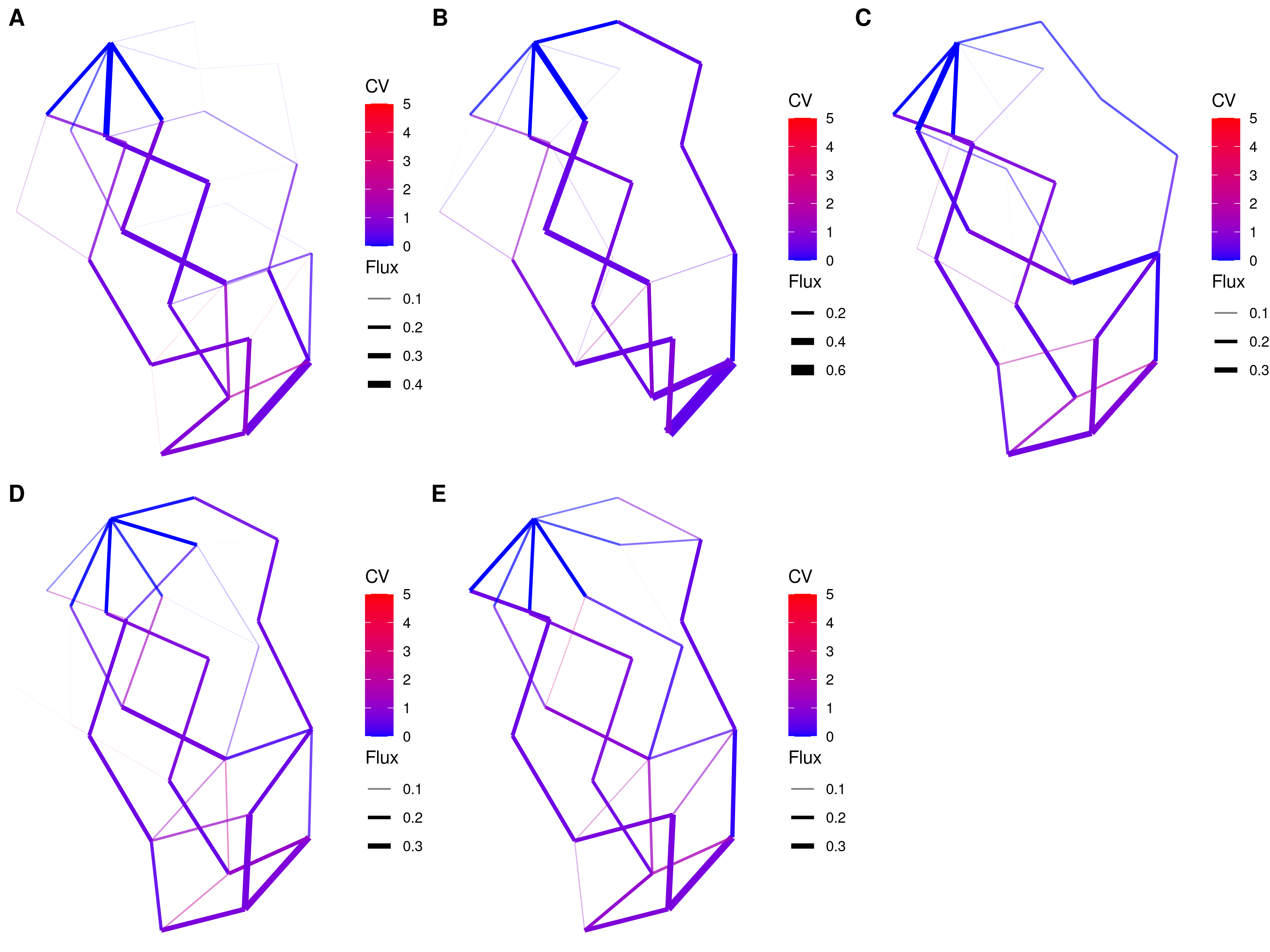
Figure 7: The learned pathways for the second dataset used in section 3.1 under model $F$, but with approximately 50% randomly inserted uncertainty markers in A: feature 2, B: feature 3, C: feature 4, D: feature 5, E: feature 6. The strength of the flux is indicated by the edge-width and the CV is marked by the colour of the edges.

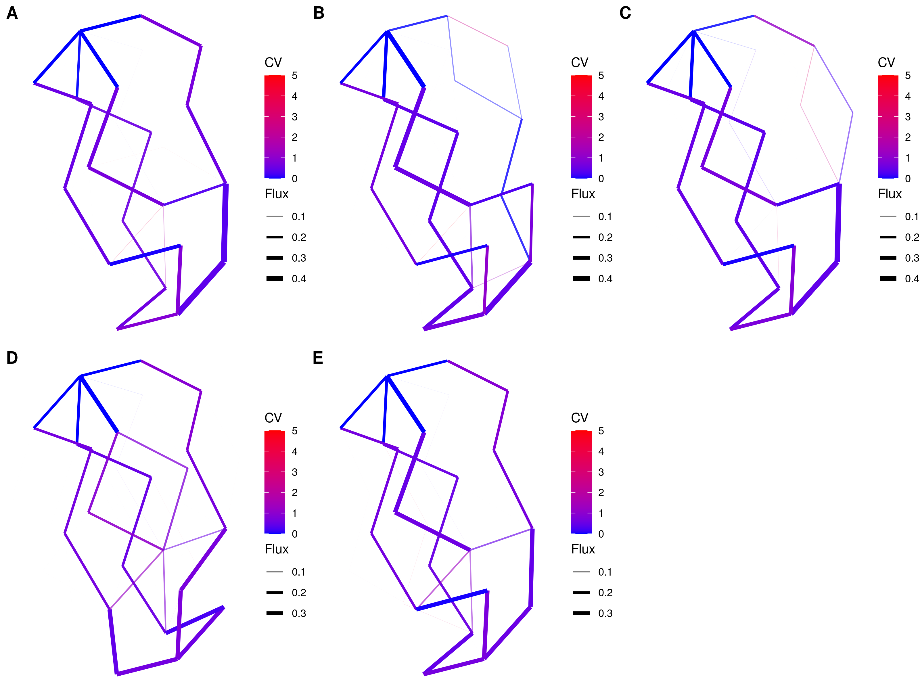
Figure 8: The learned pathways for the second dataset used in section 3.1 under model 2, but with approximately 40% randomly inserted uncertainty markers in A: feature 1, B: feature 2, C: feature 4, D: feature 5, E: feature 6. The strength of the flux is indicated by the edge-width and the CV is marked by the colour of the edges.

Figure 9: Progression of the best log-likelihood found until then of the reduced tuberculosis dataset without uncertainties and the dataset with approximately 50% randomly inserted uncertainty markers during the SA process. The iteration number on the x-axes indicates the iteration number in the optimization.

References

- [Aga et al., 2024] Aga, O. N. L., Brun, M., Dauda, K. A., Diaz-Uriarte, R., Giannakis, K., and Johnston, I. G. (2024). HyperTraPS-CT: Inference and prediction for accumulation pathways with flexible data and model structures. PLOS Computational Biology, 20(9):e1012393.
- [Beerenwinkel et al., 2006] Beerenwinkel, N., Eriksson, N., and Sturmfels, B. (2006). Evolution on distributive lattices. Journal of Theoretical Biology, 242(2):409–420.
- [Beerenwinkel et al., 2007] Beerenwinkel, N., Eriksson, N., and Sturmfels, B. (2007). Conjunctive Bayesian networks. Bernoulli, 13(4):893–909.
- [Beerenwinkel et al., 2015] Beerenwinkel, N., Schwarz, R. F., Gerstung, M., and Markowetz, F. (2015). Cancer Evolution: Mathematical Models and Computational Inference. Systematic Biology, 64(1):e1–e25.
- [Beerenwinkel and Sullivant, 2009] Beerenwinkel, N. and Sullivant, S. (2009). Markov models for accumulating mutations. Biometrika, 96(3):645–661.
- [Casali et al., 2014] Casali, N., Nikolayevskyy, V., Balabanova, Y., Harris, S. R., Ignatyeva, O., Kontsevaya, I., Corander, J., Bryant, J., Parkhill, J., Nejentsev, S., Horstmann, R. D., Brown, T., and Drobniewski, F. (2014). Evolution and transmission of drug-resistant tuberculosis in a Russian population. Nature Genetics, 46(3):279–286.
- [Chen, 2023] Chen, J. (2023). Timed hazard networks: Incorporating temporal difference for oncogenetic analysis. PLOS ONE, 18(3):e0283004.
- [Csardi and Nepusz, 2006] Csardi, G. and Nepusz, T. (2006). The igraph software package for complex network research. InterJournal, Complex Systems:1695.
- [Csárdi et al., 2024] Csárdi, G., Nepusz, T., Traag, V., Horvát, S., Zanini, F., Noom, D., and Müller, K. (2024). {igraph}: Network Analysis and Visualization in R.
- [Dalgıç et al., 2021] Dalgıç, Ö. O., Wu, H., Safa Erenay, F., Sir, M. Y., Özaltın, O. Y., Crum, B. A., and Pasupathy, K. S. (2021). Mapping of critical events in disease progression through binary classification: Application to amyotrophic lateral sclerosis. Journal of Biomedical Informatics, 123:103895.
- [Desper et al., 1999] Desper, R., Jiang, F., Kallioniemi, O.-P., Moch, H., Papadimitriou, C. H., and Schäffer, A. A. (1999). Inferring Tree Models for Oncogenesis from Comparative Genome Hybridization Data. Journal of Computational Biology, 6(1):37–51.
- [Diaz-Uriarte, 2023] Diaz-Uriarte, R. (2023). A picture guide to cancer progression and monotonic accumulation models: evolutionary assumptions, plausible interpretations, and alternative uses. arXiv. Preprint. http://arxiv.org/abs/2312.06824.
- [Diaz-Uriarte and Vasallo, 2019] Diaz-Uriarte, R. and Vasallo, C. (2019). Every which way? On predicting tumor evolution using cancer progression models. PLOS Computational Biology, 15(8):e1007246.
- [Gao et al., 2022] Gao, Y., Gaither, J., Chifman, J., and Kubatko, L. (2022). A phylogenetic approach to inferring the order in which mutations arise during cancer progression. PLOS Computational Biology, 18(12):e1010560.
- [Gerstung et al., 2009] Gerstung, M., Baudis, M., Moch, H., and Beerenwinkel, N. (2009). Quantifying cancer progression with conjunctive Bayesian networks. Bioinformatics, 25(21):2809–2815.
- [Gotovos et al., 2021] Gotovos, A., Burkholz, R., Quackenbush, J., and Jegelka, S. (2021). Scaling up Continuous-Time Markov Chains Helps Resolve Underspecification. In Advances in Neural Information Processing Systems, volume 34, pages 14580–14592. Curran Associates, Inc.
- [Greenbury et al., 2020] Greenbury, S. F., Barahona, M., and Johnston, I. G. (2020). HyperTraPS: Inferring Probabilistic Patterns of Trait Acquisition in Evolutionary and Disease Progression Pathways. Cell Systems, 10(1):39–51.e10.
- [Hjelm et al., 2006] Hjelm, M., Höglund, M., and Lagergren, J. (2006). New Probabilistic Network Models and Algorithms for Oncogenesis. Journal of Computational Biology, 13(4):853–865.
- [Johnston and Diaz-Uriarte, 2024] Johnston, I. G. and Diaz-Uriarte, R. (2024). A hypercubic Mk model framework for capturing reversibility in disease, cancer, and evolutionary accumulation modelling. bioRxiv. Preprint. https://www.biorxiv.org/content/10.1101/2024.06.27.600959v1.
- [Johnston et al., 2019] Johnston, I. G., Hoffmann, T., Greenbury, S. F., Cominetti, O., Jallow, M., Kwiatkowski, D., Barahona, M., Jones, N. S., and Casals-Pascual, C. (2019). Precision identification of high-risk phenotypes and progression pathways in severe malaria without requiring longitudinal data. npj Digital Medicine, 2(1):1–9.
- [Johnston and Williams, 2016] Johnston, I. G. and Williams, B. P. (2016). Evolutionary Inference across Eukaryotes Identifies Specific Pressures Favoring Mitochondrial Gene Retention. Cell Systems, 2(2):101–111.
- [Kassambara, 2023] Kassambara, A. (2023). ggpubr: ’ggplot2’ Based Publication Ready Plots. R package version 0.6.0.
- [Lewis, 2001] Lewis, P. O. (2001). A Likelihood Approach to Estimating Phylogeny from Discrete Morphological Character Data. Systematic Biology, 50(6):913–925.
- [Luo et al., 2023] Luo, X. G., Kuipers, J., and Beerenwinkel, N. (2023). Joint inference of exclusivity patterns and recurrent trajectories from tumor mutation trees. Nature Communications, 14(1):3676.
- [Maier et al., 2013] Maier, U.-G., Zauner, S., Woehle, C., Bolte, K., Hempel, F., Allen, J. F., and Martin, W. F. (2013). Massively Convergent Evolution for Ribosomal Protein Gene Content in Plastid and Mitochondrial Genomes. Genome Biology and Evolution, 5(12):2318–2329.
- [Moen and Johnston, 2023] Moen, M. T. and Johnston, I. G. (2023). HyperHMM: efficient inference of evolutionary and progressive dynamics on hypercubic transition graphs. Bioinformatics, 39(1):btac803.
- [Montazeri et al., 2016] Montazeri, H., Kuipers, J., Kouyos, R., Böni, J., Yerly, S., Klimkait, T., Aubert, V., Günthard, H. F., Beerenwinkel, N., and The Swiss HIV Cohort Study (2016). Large-scale inference of conjunctive Bayesian networks. Bioinformatics, 32(17):i727–i735.
- [Murray et al., 2022] Murray, C. J. L., Ikuta, K. S., Sharara, F., Swetschinski, L., Robles Aguilar, G., Gray, A., Han, C., Bisignano, C., Rao, P., Wool, E., Johnson, S. C., Browne, A. J., Chipeta, M. G., Fell, F., Hackett, S., Haines-Woodhouse, G., Kashef Hamadani, B. H., Kumaran, E. A. P., McManigal, B., Achalapong, S., Agarwal, R., Akech, S., Albertson, S., Amuasi, J., Andrews, J., Aravkin, A., Ashley, E., Babin, F.-X., Bailey, F., Baker, S., Basnyat, B., Bekker, A., Bender, R., Berkley, J. A., Bethou, A., Bielicki, J., Boonkasidecha, S., Bukosia, J., Carvalheiro, C., Castañeda-Orjuela, C., Chansamouth, V., Chaurasia, S., Chiurchiù, S., Chowdhury, F., Clotaire Donatien, R., Cook, A. J., Cooper, B., Cressey, T. R., Criollo-Mora, E., Cunningham, M., Darboe, S., Day, N. P. J., De Luca, M., Dokova, K., Dramowski, A., Dunachie, S. J., Duong Bich, T., Eckmanns, T., Eibach, D., Emami, A., Feasey, N., Fisher-Pearson, N., Forrest, K., Garcia, C., Garrett, D., Gastmeier, P., Giref, A. Z., Greer, R. C., Gupta, V., Haller, S., Haselbeck, A., Hay, S. I., Holm, M., Hopkins, S., Hsia, Y., Iregbu, K. C., Jacobs, J., Jarovsky, D., Javanmardi, F., Jenney, A. W. J., Khorana, M., Khusuwan, S., Kissoon, N., Kobeissi, E., Kostyanev, T., Krapp, F., Krumkamp, R., Kumar, A., Kyu, H. H., Lim, C., Lim, K., Limmathurotsakul, D., Loftus, M. J., Lunn, M., Ma, J., Manoharan, A., Marks, F., May, J., Mayxay, M., Mturi, N., Munera-Huertas, T., Musicha, P., Musila, L. A., Mussi-Pinhata, M. M., Naidu, R. N., Nakamura, T., Nanavati, R., Nangia, S., Newton, P., Ngoun, C., Novotney, A., Nwakanma, D., Obiero, C. W., Ochoa, T. J., Olivas-Martinez, A., Olliaro, P., Ooko, E., Ortiz-Brizuela, E., Ounchanum, P., Pak, G. D., Paredes, J. L., Peleg, A. Y., Perrone, C., Phe, T., Phommasone, K., Plakkal, N., Ponce-de Leon, A., Raad, M., Ramdin, T., Rattanavong, S., Riddell, A., Roberts, T., Robotham, J. V., Roca, A., Rosenthal, V. D., Rudd, K. E., Russell, N., Sader, H. S., Saengchan, W., Schnall, J., Scott, J. A. G., Seekaew, S., Sharland, M., Shivamallappa, M., Sifuentes-Osornio, J., Simpson, A. J., Steenkeste, N., Stewardson, A. J., Stoeva, T., Tasak, N., Thaiprakong, A., Thwaites, G., Tigoi, C., Turner, C., Turner, P., van Doorn, H. R., Velaphi, S., Vongpradith, A., Vongsouvath, M., Vu, H., Walsh, T., Walson, J. L., Waner, S., Wangrangsimakul, T., Wannapinij, P., Wozniak, T., Young Sharma, T. E. M. W., Yu, K. C., Zheng, P., Sartorius, B., Lopez, A. D., Stergachis, A., Moore, C., Dolecek, C., and Naghavi, M. (2022). Global burden of bacterial antimicrobial resistance in 2019: a systematic analysis. The Lancet, 399(10325):629–655.
- [Nichol et al., 2015] Nichol, D., Jeavons, P., Fletcher, A. G., Bonomo, R. A., Maini, P. K., Paul, J. L., Gatenby, R. A., Anderson, A. R. A., and Scott, J. G. (2015). Steering Evolution with Sequential Therapy to Prevent the Emergence of Bacterial Antibiotic Resistance. PLOS Computational Biology, 11(9):e1004493.
- [Nicol et al., 2021] Nicol, P. B., Coombes, K. R., Deaver, C., Chkrebtii, O., Paul, S., Toland, A. E., and Asiaee, A. (2021). Oncogenetic network estimation with disjunctive Bayesian networks. Computational and Systems Oncology, 1(2):e1027.
- [Pagel, 1994] Pagel, M. (1994). Detecting correlated evolution on phylogenies: a general method for the comparative analysis of discrete characters. Proceedings of the Royal Society, 255(1342):37–45.
- [Pedersen, 2024] Pedersen, T. L. (2024). ggraph: An Implementation of Grammar of Graphics for Graphs and Networks.
- [Renz et al., 2024] Renz, J., Dauda, K. A., Aga, O. N. L., Diaz-Uriarte, R., Löhr, I. H., Blomberg, B., and Johnston, I. G. (2024). Evolutionary accumulation modelling in AMR: machine learning to infer and predict evolutionary dynamics of multi-drug resistance. arXiv. Preprint. http://arxiv.org/abs/2411.00219.
- [Revell, 2024] Revell, L. J. (2024). phytools 2.0: an updated R ecosystem for phylogenetic comparative methods ( and other things). PeerJ, 12:e16505.
- [Rupp et al., 2024] Rupp, K., Schill, R., Süskind, J., Georg, P., Klever, M., Lösch, A., Grasedyck, L., Wettig, T., and Spang, R. (2024). Differentiated uniformization: a new method for inferring Markov chains on combinatorial state spaces including stochastic epidemic models. Computational Statistics.
- [Sanderson and Curtin, 2016] Sanderson, C. and Curtin, R. (2016). Armadillo: a template-based C++ library for linear algebra. Journal of Open Source Software, 1(2):26.
- [Sanderson and Curtin, 2019] Sanderson, C. and Curtin, R. (2019). Practical Sparse Matrices in C++ with Hybrid Storage and Template-Based Expression Optimisation. Mathematical and Computational Applications, 24(3).
- [Schill et al., 2024a] Schill, R., Klever, M., Lösch, A., Hu, Y. L., Vocht, S., Rupp, K., Grasedyck, L., Spang, R., and Beerenwinkel, N. (2024a). Overcoming Observation Bias for Cancer Progression Modeling. In Ma, J., editor, Research in Computational Molecular Biology, pages 217–234, Cham. Springer Nature Switzerland.
- [Schill et al., 2024b] Schill, R., Klever, M., Rupp, K., Hu, Y. L., Lösch, A., Georg, P., Pfahler, S., Vocht, S., Hansch, S., Wettig, T., Grasedyck, L., and Spang, R. (2024b). Reconstructing Disease Histories in Huge Discrete State Spaces. KI - Künstliche Intelligenz.
- [Schill et al., 2020] Schill, R., Solbrig, S., Wettig, T., and Spang, R. (2020). Modelling cancer progression using Mutual Hazard Networks. Bioinformatics, 36(1):241–249.
- [Schliep, 2011] Schliep, K. (2011). phangorn: phylogenetic analysis in R. Bioinformatics, 27(4):592–593.
- [Schliep et al., 2017] Schliep, K., Potts, A., Morrison, D. A., and Grimm, G. W. (2017). Intertwining phylogenetic trees and networks. Methods in Ecology and Evolution, 8(10):1212–1220.
- [Schwartz and Schäffer, 2017] Schwartz, R. and Schäffer, A. A. (2017). The evolution of tumour phylogenetics: principles and practice. Nature Reviews Genetics, 18(4):213–229.
- [Szabo and Boucher, 2002] Szabo, A. and Boucher, K. (2002). Estimating an oncogenetic tree when false negatives and positives are present. Mathematical Biosciences, 176(2):219–236.
- [Takeshima and Ushijima, 2019] Takeshima, H. and Ushijima, T. (2019). Accumulation of genetic and epigenetic alterations in normal cells and cancer risk. npj Precision Oncology, 3(1):1–8.
- [Tan et al., 2011] Tan, L., Serene, S., Chao, H. X., and Gore, J. (2011). Hidden Randomness between Fitness Landscapes Limits Reverse Evolution. Physical Review Letters, 106(19):198102.
- [Wickham, 2016] Wickham, H. (2016). ggplot2: Elegant Graphics for Data Analysis. Springer-Verlag New York.
- [Wickham, 2023] Wickham, H. (2023). stringr: Simple, Consistent Wrappers for Common String Operations.
- [Wickham et al., 2023] Wickham, H., François, R., Henry, L., Müller, K., and Vaughan, D. (2023). dplyr: A Grammar of Data Manipulation. R package version 1.1.4, https://github.com/tidyverse/dplyr, https://dplyr.tidyverse.org.
- [Youn and Simon, 2012] Youn, A. and Simon, R. (2012). Estimating the order of mutations during tumorigenesis from tumor genome sequencing data. Bioinformatics, 28(12):1555–1561.