Symmetric Tensor Coupling in Holographic Mean-Field Theory: Deformed Dirac Cones

Abstract

We extend the holographic mean-field theory to rank-two symmetric tensor order parameter field coupled with fermion. We classify the roles of symmetric tensor order according to the effect on the spectral density: cone-angle change, squashing, and tilting of the spectral light cones. In case of the over-tilted light cone, an analytic continuation of the Green’s function is necessary to preserve the continuity of the spectrum inside the lightcone. Our results provide agreements between the holographic spectra with those observed in real materials, such as type-II Dirac cones and strained graphene.

1 Introduction

The AdS/CFT correspondence has offered a powerful way to investigate strongly coupled quantum systems by examining their dual classical gravity dual Maldacena:1997re ; Witten:1998qj . Early studies of holography provided the set up to calculate the retarded Green’s functions and revealed the basic aspects of dynamics in boundary theories. Subsequently, the method has been widely used in condensed matter systems, most notably in transports Hartnoll:2009sz ; Faulkner:2009wj ; Faulkner:2010da ; Donos:2013eha ; Blake:2013bqa ; Donos:2014yya ; Kim:2014bza ; Davison_2014 ; Blake_2015 ; Hartnoll:2016apf ; Ge:2016lyn ; Donos:2018kkm and holographic superconductors Hartnoll:2008kx ; Hartnoll:2008vx ; Gubser:2008px ; Faulkner:2009am ; Horowitz_2009 ; Horowitz_2011 ; Kim:2013oba as well as fermion dynamics Iqbal:2009fd ; laia2011holographic ; Faulkner:2013bna .

Motivated by these developments, holographic mean-field theory (HMFT) was developed systematically as an effective method to incorporate the basic features of the fermion spectrum Oh:2020cym ; Sukrakarn:2023ncp appearing in the ARPES data of real fermion: by introducing order parameters $B_{A_{1}A_{2}A_{3}\cdots}$ that break symmetries in the bulk spacetime through fermionic bilinear couplings of the form

$$\mathcal{L}_{\mathrm{int}}=B_{A_{1}A_{2}A_{3}\cdots}\bar{\psi}\Gamma^{A_{1}A_{2}A_{3}\cdots}\psi,$$ (1)

it was observed that the holographic Green’s functions contains many of the features in the spectral functions of the fermions in the real system so that it was suggested that Sukrakarn:2023ncp the order parameter field due to the specific symmetry breaking could be used as a way to encode the effect of certain lattices. Naturally such scheme was applied to various types of holographic superconductors Yuk:2022lof ; Ghorai:2023wpu ; PhysRevD.109.066004 as well as to the Kondo lattice physics Im:2023ffg ; Han:2024rbr .

In Oh:2020cym ; Sukrakarn:2023ncp , the order parameters of scalar,vector, and antisymmetric tensor types were considered the results were classified, but the symmetric tensor coupling,

$$\mathcal{L}_{\mathrm{int}}=h_{MN}\bar{\psi}\Gamma^{(M}D^{N)}\psi,$$ (2)

with $h_{MN}$ being the rank-2 symmetric tensor field, was not considered. Also previous literature on symmetric tensors primarily focused on purely spatial components ($h_{ii}$ and $h_{ij}$), identifying them with $d$-wave order parameters in holographic superconductors with gap features in spectral densities and $U(1)$-symmetry breaking are present Horowitz_2009 ; Horowitz_2011 ; Kim:2013oba ; PhysRevD.109.066004 . Traceless spatial symmetric tensors were also studied and associated with quantum spin nematic phases PhysRevB.64.195109 ; PhysRevB.96.235140 , realized through linearized gravity PhysRevB.109.L220407 . However, the effects of time-time ($h_{tt}$), time-space ($h_{ti}$) has not been considered and general correspondence of the symmetric tensor and their counterparts in condensed matter systems have not been identified.

This work seeks to bridge the gap in understanding by systematically analyzing the effects of all tensor components from the view of the holographic mean-field theory (HMFT) framework: we extend HMFT by coupling one- and two-flavor spinors to a rank-two symmetric tensor in $\mathrm{AdS}_{5}$, providing analytic evaluations of Green’s functions and spectral densities (SDs) at the level of the probe without full backreaction.

It turns out that boundary components of the symmetric tensor field $h_{\mu\nu}$ coupled to Dirac spinors induce three distinct types of deformations in the resulting spectral densities: cone-angle change, squashing, and tilting. We present these possibilities schematically as follows:

$$h_{\mu\nu}=\begin{pmatrix}\pagecolor{yellow!20}h_{tt}&\pagecolor{blue!20}h_{tx}&\pagecolor{blue!20}h_{ty}&\pagecolor{blue!20}h_{tz}\\ \pagecolor{blue!20}h_{tx}&\pagecolor{red!20}h_{xx}&\pagecolor{red!20}h_{xy}&\pagecolor{red!20}h_{xz}\\ \pagecolor{blue!20}h_{ty}&\pagecolor{red!20}h_{xy}&\pagecolor{red!20}h_{yy}&\pagecolor{red!20}h_{yz}\\ \pagecolor{blue!20}h_{tz}&\pagecolor{red!20}h_{xz}&\pagecolor{red!20}h_{yz}&\pagecolor{red!20}h_{zz}\\ \end{pmatrix}\quad\text{where}\quad\left\{\begin{aligned} &\fcolorbox{black}{yellow!20}{\rule{0pt}{6pt}\rule{6pt}{0pt}}:\,\text{Cone-angle change},\\ &\fcolorbox{black}{red!20}{\rule{0pt}{6pt}\rule{6pt}{0pt}}:\,\text{Squashing},\\ &\fcolorbox{black}{blue!20}{\rule{0pt}{6pt}\rule{6pt}{0pt}}:\,\text{Tilting}+\text{Squashing}.\end{aligned}\right.$$ (3)

These symmetric tensor couplings can therefore reshape the spectral densities in various ways, with each component of $h_{\mu\nu}$ serving as a parameter that modifies Fermi velocities or induces tilts in specific direction.

It is remarkable that each symmetric tensor component can find a corresponding real system parameter counterpart in condensed matter systems. The strength of $h_{\mu\nu}$ can be associated with specific parameters in condensed matter systems by analyzing the spectral features under the symmetric tensor coupling.

For instance, the $h_{tt}$ component induces cone-angle change of the spectral densities, leading to the modification of the Fermi velocity under a uniform electric field D_az_Fern_ndez_2017 . Also, critically decreased Fermi velocity due to strong $h_{tt}$ coupling can be associated with the local flat band near the Dirac point observed in twisted bilayer graphene at the magic angle Lisi_2020 .

In the case of $h_{ti}$, the coupling induces a tilting of the SDs, which can be interpreted as a tilt parameter, leading to type-I, type-II, or type-III Dirac cones PhysRevX.9.031010 according to the coupling strength. For two flavour system, such classification leads to the corresponding Weyl semimetals Soluyanov_2015 of type-I, -II, -III. It turns out that such tilts can be realized through metric deformations and modifications of the Lorentz algebra Volovik_2016 ; Volovik_2021 ; PhysRevResearch.4.033237 ; PhysRevB.100.045144 , which will be reported in a separate publicationJW_2025 .

On the other hand, the spatial components $h_{ii}$ and $h_{ij}$ induce squashing, i.e, anisotropic scaling, on spectral density in momentum space. We can identify these spatial components as the rank-2 quadrupole order parameters of quantum spin nematic phases which also give rise to elliptical Fermi surfaces PhysRevB.64.195109 ; PhysRevB.96.235140 . Indeed, the effects of $h_{ij}$ resemble lattice deformations, such as strain and shear strain, described by a rank-2 strain tensor and observed in systems like strained and twisted (bilayer) graphene PhysRevB.88.085430 ; PhysRevResearch.4.L022027 , as well as in $\mathrm{Bi}_{2}\mathrm{Se}_{3}$-class materials Brems_2018 ; PhysRevB.84.195425 .

We summarize the correspondence between the symmetric tensor coupling and the real material examples in condensed matter in the table 1.

Order Types	Features in Holographic SD	Phenomena in Real Systems	System Parameter
$h_{tt}$	Cone-angle change	Tuning Fermi velocity in Dirac materials via a uniform electric field D_az_Fern_ndez_2017 .	Electric field
		Flat bands at local Dirac points emerge in twisted bilayer graphene at the magic angle Lisi_2020 .	Twist angle
$h_{ti}$	Tilting and squashing	Rotated energy dispersion in tilted type-I, type-II, and type-III Dirac/Weyl cones PhysRevX.9.031010 .	Tilt parameter
$h_{ii}$, $h_{ij}$	Squashing and rotation	Spatial components of symmetric tensor couplings identified as $d$-wave order parameters for holographic superconductors if there is a gap feature Kim:2013oba ; PhysRevD.109.066004 .	$d$-wave order parameters
		Quadrupolar two-rank tensors for quantum spin nematic phases PhysRevB.64.195109 ; PhysRevB.96.235140 , which can be realized by linearized gravity PhysRevB.109.L220407 .	Nematic order parameter
		Lattice deformation (strain and shear strain) in (bilayer) graphene PhysRevB.88.085430 ; PhysRevResearch.4.L022027 and $\mathrm{Bi}_{2}\mathrm{Se}_{3}$ Brems_2018 .	Strain tensor
		Anisotropic deformation of Dirac cones of superlattice graphene due to a periodic potential Park_2008 .	Superlattice structure

Table 1: Summary: Classification of symmetric tensor coupling components, their spectral features and examples in condensed matter systems.

Notice that the $h_{\mu\nu}$ components can be identified by matching measured Fermi velocities, cone angles, and tilting angles of the local energy dispersion for a given material, which constitute our primary results. For instance, figure 1 shows the band structure of graphene Katsnelson_2020 as an illustrative example of a Dirac dispersion that could be both qualitatively and quantitatively associated with symmetric tensor couplings at each local crossing point.

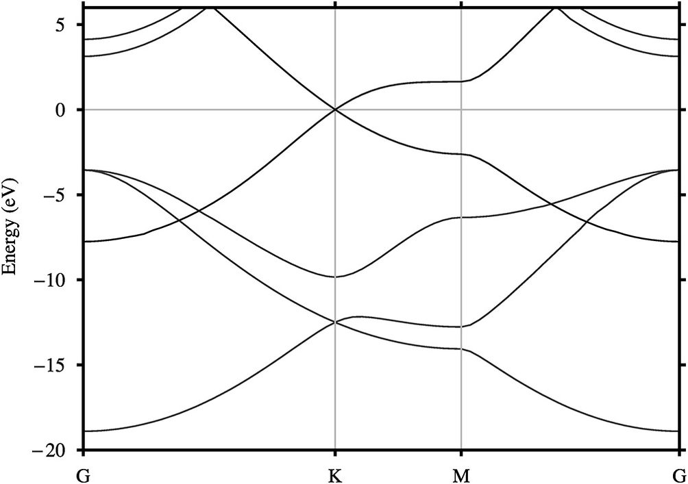
Figure 1: Graphene band structure, adapted from Katsnelson_2020 . Lattice deformations or interactions can reshape the Dirac cones in ways that may be effectively described by and identified with the effects of symmetric tensor couplings $h_{\mu\nu}$ on spectral densities.

The rest of this paper is organized as follows. In section 2, we define the bulk and boundary actions, introduce the symmetric tensor coupling, and derive the Dirac equation for holographic fermions. Sections 3 to 4 derive analytic retarded Green’s functions for one- and two-flavor spinors, categorizing the resulting spectral densities based on their scaling and rotational behavior under each $h_{\mu\nu}$ component. In section 5, we investigate over-tilted spectral densities and propose a formalism to ensure their well-defined nature. In section 6, we explore potential applications of the symmetric tensor coupling by comparing its components with analogous parameters in condensed matter systems. Finally, section 7 summarizes the main findings and discusses potential applications of this holographic mean-field theory approach to other condensed matter systems.

2 Holographic fermions with symmetric tensor coupling

We set up the notations for holographic fermions. Throughout this paper, $M,N,\cdots$ or $t,x,\cdots$ represent bulk indices on a five-dimensional manifold $\mathcal{M}$, while $a,b,\cdots$ or $\underline{t},\underline{x},\cdots$ denote the local tangent space indices in the vielbein formalism. Additionally, the indices $\mu,\nu,\cdots$ represent boundary indices on a four-dimensional $\partial\mathcal{M}$, while $i,j,\cdots$ denotes the spatial indices at the boundary. Now we define the action by

$$S_{\mathrm{tot}}=S_{\mathrm{bulk}}+S_{\mathrm{bdy}}+S_{g}+S_{\mathrm{int}},$$ (4)

$$S_{\mathrm{bulk}}=i\int_{\mathcal{M}}d^{5}x\sqrt{-g}\,\bar{\psi}(\overleftrightarrow{\not{D}}-m)\psi,$$ (5)

$$S_{\mathrm{bdy}}=i\int_{\partial\mathcal{M}}d^{4}x\sqrt{-gg^{rr}}\bar{\psi}\psi,$$ (6)

$$S_{g}=\int_{\mathcal{M}}d^{5}x\sqrt{-g}\left(R-2\Lambda\right),$$ (7)

$$S_{\mathrm{int}}=i\int_{\mathcal{M}}d^{5}x\sqrt{-g}\bar{\psi}h_{MN}\Gamma^{(M}D^{N)}\psi.$$ (8)

Here, $\overleftrightarrow{\not{D}}=\frac{1}{2}(\overrightarrow{\not{D}}-\overleftarrow{\not{D}})$, where $\not{D}=\Gamma^{M}D_{M}=\Gamma^{M}\left(\partial_{M}+\frac{1}{4}\omega_{abM}\Gamma^{ab}\right)$, and $\omega_{abM}$ denotes the spin connection. The field $g_{MN}$ is the background metric tensor associated with the cosmological constant $\Lambda$, whereas $h_{MN}$ represents a five-dimensional symmetric rank-2 tensor. In (6), $g^{rr}$ denotes the radial-radial component of the inverse metric. In this paper, we consider fermions in the probe limit.

We introduce the order parameter field $h_{MN}(r)$ in the form of a symmetric tensor, as given in (8), with the indices $M,N=t,x,y,z,r$. Throughout this paper, we particularly focus on the boundary components of $h_{MN}(r)$, defined as

$$h_{\mu\nu}(r)=\left.h_{MN}(r)\right|_{M,N\,=\,t,x,y,z}.$$ (9)

For simplicity, we occasionally denote this as $h_{\mu\nu}$. To ensure our model for interacting spinors is analytically solvable, we set the ansatz for (9) to a leading-order mean-field approximation, where the symmetric tensor minimally couples to the fermions, such that

$$h_{\mu\nu}(r)=\varphi_{\mu\nu}/r^{2}=\frac{1}{r^{2}}\begin{pmatrix}\varphi_{tt}&\varphi_{tx}&\varphi_{ty}&\varphi_{tz}\\ \varphi_{tx}&\varphi_{xx}&\varphi_{xy}&\varphi_{xz}\\ \varphi_{ty}&\varphi_{xy}&\varphi_{yy}&\varphi_{yz}\\ \varphi_{tz}&\varphi_{xz}&\varphi_{yz}&\varphi_{zz}\end{pmatrix},$$ (10)

where $\varphi_{\mu\nu}$ are constant parameters that characterize the strength of the symmetric tensor coupling. Until section 4, we assume $|\varphi_{\mu\nu}|<1$ for simplicity in examining the effects on spectral densities. In section 5, we will examine the case $|\varphi_{ti}|\geq 1$, which gives rise to critically tilted and over-tilted spectral densities.

3 One-flavor spinor

This section applies the holographic framework from section 2 to derive the analytic retarded Green’s function for a one-flavor spinor under symmetric tensor coupling. We further examine how this coupling induces scaling and rotational deformations in the spectral densities, providing a classification of symmetric tensor couplings based on their effects on the spectral density.

3.1 Dirac equation and source identification

Throughout this paper, we adopt the gamma matrix representation as

$$\begin{gathered}\Gamma^{\underline{t}}=-i\sigma_{1}\otimes\mathbbm{1}_{2\times 2},\quad\Gamma^{\underline{x}}=\sigma_{2}\otimes\sigma_{1},\quad\Gamma^{\underline{y}}=\sigma_{2}\otimes\sigma_{2},\quad\Gamma^{\underline{z}}=\sigma_{2}\otimes\mathbbm{1}_{2\times 2},\quad\\ \Gamma^{\underline{r}}=\sigma_{3}\otimes\mathbbm{1}_{2\times 2},\quad\Gamma^{ab}=\frac{1}{2}[\Gamma^{a},\Gamma^{b}].\end{gathered}$$ (11)

The gamma matrices satisfy the Clifford algebra $[\Gamma^{M},\Gamma^{N}]=2g^{MN}\mathbbm{1}_{5\times 5}$ in five dimension so that $\Gamma^{MN}$ contains some metric dependence. We define the metric of the bulk in the inverse radius coordinate as

$$ds^{2}=-\frac{f(r)}{r^{2}}dt^{2}+\frac{dx^{2}+dy^{2}+dz^{2}}{r^{2}}+\frac{dr^{2}}{r^{2}f(r)},$$ (12)

which is asymptotically $\mathrm{AdS}_{5}$. Also, in (7), $\Lambda=-6$ and we set the $\mathrm{AdS}_{5}$ radius to 1 throughout this paper. From the total action in (4), we can write down the bulk equation of motion for $\psi$ as

$$\begin{gathered}(\Gamma^{M}D_{M}-m)\psi+h_{MN}\Gamma^{(M}D^{N)}\psi=[(g+h)_{MN}\Gamma^{M}D^{N}-m]\psi=0,\end{gathered}$$ (13)

We put an ansatz of Dirac field as

$$\psi=(-gg^{rr})^{-1/4}e^{-i\omega t+ik_{x}x+ik_{y}y+ik_{z}z}\zeta(r),$$ (14)

where $\zeta(r)$ is a four-component spinor field. The term $(-gg^{rr})^{-1/4}$ was introduced to remove spin-connection term in Dirac equation, which greatly simplifies the system. For instance, in pure $\mathrm{AdS}_{5}$ geometry with the symmetric tensor given by (10), the Dirac equation is

$$\begin{gathered}\Gamma^{\underline{r}}\partial_{r}\zeta(r)+ir^{2}\Gamma^{\mu}(g+h)_{\mu\nu}k^{\nu}\zeta(r)-\dfrac{\mathrm{Tr}h}{2r}\Gamma^{\underline{r}}\zeta(r)-\dfrac{m}{r}\zeta(r)=0,\\ \text{where}\quad k^{\mu}=(\omega,\boldsymbol{k})=(\omega,k_{x},k_{y},k_{z})\quad\text{and}\quad\mathrm{Tr}h=g^{\mu\nu}h_{\mu\nu}(r).\end{gathered}$$ (15)

Notice that the order parameter field $h_{\mu\nu}$ could be considered as a metric perturbation. We will utilize this equation of motion when applying the flow equation and defining the retarded Green’s function in pure $\mathrm{AdS}_{5}$ system.

To define the retarded Green’s function, we first identify the source and condensation. For this, we decompose the spinor field in (14) as

$$\psi=\begin{pmatrix}\psi_{+}\\ \psi_{-}\end{pmatrix}\quad\text{and}\quad\zeta=\begin{pmatrix}\zeta_{+}\\ \zeta_{-}\end{pmatrix}.$$ (16)

Then, by applying the ansatz (14), the boundary action in (6) can be rewritten as

$$\begin{gathered}S_{\mathrm{bdy}}=i\int_{\partial\mathcal{M}}d^{4}x\bar{\zeta}\zeta=\int_{\partial\mathcal{M}}d^{4}x\zeta^{\dagger}(\sigma_{1}\otimes\sigma_{0})\zeta=\int_{\partial\mathcal{M}}d^{4}x\,\zeta^{\dagger}_{+}\zeta_{-}+\mathrm{h.c.}\end{gathered}$$ (17)

By varying the bulk action with respect to $\psi$ and add the variation of the first term in (17), it can be shown that the total action variation can be represented only in terms of $\zeta_{+}$ if the equation of motion is satisfied Iqbal:2009fd . Therefore, we interpret the boundary quantities of $\zeta_{+}$ and $\zeta_{-}$ as the two-component source and condensation, respectively. For notational clarity, we redefine the bulk quantities $\zeta_{+}$ and $\zeta_{-}$ as $\xi^{(S)}$ and $\xi^{(C)}$, respectively, corresponding to the source and condensation at the boundary:

$$\xi^{(S)}\equiv\zeta_{+}\quad\text{and}\quad\xi^{(C)}\equiv\zeta_{-}.$$ (18)

To find the retarded Green’s function, we extract the source and condensation terms from their corresponding bulk quantities, $\xi^{(S)}$ and $\xi^{(C)}$. To achieve this, we examine the boundary behavior of $\xi^{(S)}$ and $\xi^{(C)}$ by solving the Dirac equation in (13). We can represent the Dirac equation in terms of $\xi^{(S)}$ and $\xi^{(C)}$ in (18) as

$$\partial_{r}\xi^{(S)}+\mathbb{M}_{1}\xi^{(S)}+\mathbb{M}_{2}\xi^{(C)}=0,$$ (19)

$$\partial_{r}\xi^{(C)}+\mathbb{M}_{3}\xi^{(C)}+\mathbb{M}_{4}\xi^{(S)}=0.$$ (20)

where $\mathbb{M}_{1}$, $\mathbb{M}_{2}$, $\mathbb{M}_{3}$, and $\mathbb{M}_{4}$ are $2\times 2$ matrix-valued functions. We consider near-boundary behavior of $\xi^{(S)}$ and $\xi^{(C)}$ for pure $\mathrm{AdS}_{5}$ case by analytically solving (19) and (20). For spacelike spinors $|m|<1/2$, the leading $r$-dependent terms of the spinors $\xi^{(S)}$ and $\xi^{(C)}$ near the boundary are extracted as

$$\xi^{(S)}\approx r^{m+\mathrm{Tr}\varphi/2}\mathcal{J} \text{and}\quad\xi^{(C)}\approx r^{-m+\mathrm{Tr}\varphi/2}\mathcal{C},$$ (21)

$$\text{where}\quad\mathrm{Tr}\varphi=\eta^{\mu\nu}\varphi_{\mu\nu} \text{and}\quad\eta_{\mu\nu}=\mathrm{diag}(-1,1,1,1).$$

Here, $\varphi_{\mu\nu}$ is defined in (10), $\mathcal{J}$ and $\mathcal{C}$ are two-component spinors, representing the source and condensation, respectively. We will use these source and condensation terms to determine the retarded Green’s function for one-flavor spinors in the following section.

3.2 Definition of retarded Green’s function

When we define the retarded Green’s function from our chosen source and condensation, we adopt the formalism in Yuk:2022lof to express the retarded Green’s function and solve it analytically instead of solving the Dirac equation.

Because $\xi^{(S)}$ and $\xi^{(C)}$ are two-component spinors, each has two independent solutions. The general solution can therefore be expressed as a linear combination of these two solutions with constant coefficients. It is convenient to represent $\xi^{(S)}$ and $\xi^{(C)}$ in matrix form, separating the solution basis from their coefficients. For example, if we denote the two basis solutions for $\xi^{(S)}$ as $(\xi^{(S,1)}_{1},\xi^{(S,1)}_{2})^{T}$ and $(\xi^{(S,2)}_{1},\xi^{(S,2)}_{2})^{T}$, with the corresponding coefficients $c_{1}$ and $c_{2}$, then the spinor $\xi^{(S)}$ can be expressed as

$$\begin{gathered}\xi^{(S)}=c_{1}\begin{pmatrix}\xi^{(S,1)}_{1}\\ \xi^{(S,1)}_{2}\end{pmatrix}+c_{2}\begin{pmatrix}\xi^{(S,2)}_{1}\\ \xi^{(S,2)}_{2}\end{pmatrix}=\begin{pmatrix}\xi^{(S,1)}_{1}&\xi^{(S,2)}_{1}\\ \xi^{(S,1)}_{2}&\xi^{(S,2)}_{2}\end{pmatrix}\begin{pmatrix}c_{1}\\ c_{2}\end{pmatrix}=\mathbb{S}(r){\bf c},\\ \text{where}\quad\mathbb{S}(r)=\begin{pmatrix}\xi^{(S,1)}_{1}&\xi^{(S,2)}_{1}\\ \xi^{(S,1)}_{2}&\xi^{(S,2)}_{2}\end{pmatrix}\quad\text{and}\quad{\bf c}=\begin{pmatrix}c_{1}\\ c_{2}\end{pmatrix}.\end{gathered}$$ (22)

Likewise, we can represent the $\xi^{(C)}$ in a similar way. Meanwhile, due to the Dirac equations from (19) to (20), $\xi^{(C)}$ can be expressed in terms of $\xi^{(S)}$; that is, $\xi^{(C)}$ shares the same coefficient ${\bf c}$ as $\xi^{(S)}$, such that

$$\xi^{(C)}=\mathbb{C}(r){\bf c},$$ (23)

where $\mathbb{C}(r)$ is a $2\times 2$ matrix-valued function. From the boundary behavior of $\xi^{(S)}$ and $\xi^{(C)}$ in (21), we see that the leading terms $r^{\pm m+\mathrm{Tr}\varphi/2}$ of $\xi^{(S)}$ and $\xi^{(C)}$ at the boundary originate from those of $\mathbb{S}(r)$ and $\mathbb{C}(r)$ in (22) and (23), respectively, because ${\bf c}$ is a constant vector. Therefore, the boundary behavior of $\mathbb{S}(r)$ and $\mathbb{C}(r)$ is given by

$$\mathbb{S}(r)\approx r^{m+\mathrm{Tr}\varphi/2}\mathbb{S}_{0}\quad\text{and}\quad\mathbb{C}(r)\approx r^{-m+\mathrm{Tr}\varphi/2}\mathbb{C}_{0},$$ (24)

with constant matrices $\mathbb{S}_{0}$ and $\mathbb{C}_{0}$. Then, the spinors $\xi^{(S)}$ and $\xi^{(C)}$ are given by

$$\xi^{(S)}\approx r^{m+\mathrm{Tr}\varphi/2}\mathbb{S}_{0}{\bf c}\quad\text{and}\quad\xi^{(C)}\approx r^{-m+\mathrm{Tr}\varphi/2}\mathbb{C}_{0}{\bf c}.$$ (25)

Comparing (21) with (25), the source and condensation can be rewritten as

$$\mathcal{J}=\mathbb{S}_{0}{\bf c}\quad\text{and}\quad\mathcal{C}=\mathbb{C}_{0}{\bf c}\quad\hbox{ so that }\mathcal{C}=\mathbb{C}_{0}\mathbb{S}^{-1}_{0}\mathcal{J}.$$ (26)

We now can get the retarded Green’s function in terms of $\mathbb{S}_{0}$ and $\mathbb{C}_{0}$ from the total action. Meanwhile, since the bulk action does not contribute to the total action due to the equation of motion, the Green’s function is determined solely from the boundary action in (17). To achieve this, we rewrite the boundary action, which is denoted as the effective action $S_{\mathrm{eff}}$, near the boundary at $r=\epsilon$, in terms of $\mathcal{J}$ and $\mathcal{C}$ as

$$S_{\mathrm{eff}}=\int_{\partial\mathcal{M}}d^{4}x\,{\xi^{(S)}}^{\dagger}\xi^{(C)}+\mathrm{h.c.}=\int_{\partial\mathcal{M}}d^{4}x\,\epsilon^{\mathrm{Tr}\varphi}\mathcal{J}^{\dagger}\mathcal{C}+\mathrm{h.c.}$$ (27)

From the equation (26), the effective action can be rewritten in terms of the source only,

$$S_{\mathrm{eff}}=\int_{\partial\mathcal{M}}d^{4}x\,\epsilon^{\mathrm{Tr}\varphi}\mathcal{J}^{\dagger}(\mathbb{C}_{0}\mathbb{S}^{-1}_{0})\mathcal{J}+\mathrm{h.c.}$$ (28)

According to the linear response theory, the effective action can be represented as

$$S_{\mathrm{eff}}=\int_{\partial\mathcal{M}}d^{4}x\,\epsilon^{\mathrm{Tr}\varphi}\mathcal{J}^{\dagger}G_{R}\mathcal{J}+\mathrm{h.c.}$$ (29)

where $G_{R}$ is the retarded Green’s function for the source $\mathcal{J}$. By comparing (28) and (29), we identify the matrix-valued retarded Green’s function as

$$G_{R}=\mathbb{C}_{0}\mathbb{S}^{-1}_{0}.$$ (30)

On the other hand, the flow equation provides the bulk quantity $\mathbb{G}(r)$ defined by

$$\mathbb{G}(r)\equiv\mathbb{C}(r)\mathbb{S}^{-1}(r),$$ (31)

whose boundary behavior will give the retarded Green’s function $G_{R}$. Thus, to determine $G_{R}$ from $\mathbb{G}(r)$, we should look for the boundary behavior of $\mathbb{G}(r)$. From (24) and (30),

$$\mathbb{G}(r)=\mathbb{C}(r)\mathbb{S}^{-1}(r)\approx r^{-2m}\mathbb{C}_{0}\mathbb{S}^{-1}_{0}=r^{-2m}G_{R}.$$ (32)

Then, we can find the retarded Green’s function from the bulk quantity $\mathbb{G}(r)$ as

$$G_{R}=\lim_{r\to 0}r^{2m}\mathbb{G}(r)$$ (33)

Therefore, once we know $\mathbb{G}(r)$, we can calculate $G_{R}$. This is the calculational basis of our work.

Notice that from (33), we see that $\mathrm{Tr}\varphi/2$ in the boundary behavior of $\xi^{(S)}$ and $\xi^{(C)}$ does not affect to the definition of retarded Green’s function. Also, for spinors without the bulk mass, the retarded Green’s function is defined by the leading term of $\mathbb{G}(r)$ at the boundary.

3.3 Spectral densities in pure $\mathrm{AdS}_{5}$

If we find the equation satisified by $\mathbb{G}(r)$ satisfiying certain boundary condition at the horizon, we can derive the retarded Green’s function in (30) by solving it. It turns out that such equation is a first-order differential equation called flow equation PhysRevD.79.025023 ; Yuk:2022lof . We adopt the formalism in Yuk:2022lof to take the advantage that we can get the analytic Green’s function directly without explicitly solving for the spinors $\xi^{(S)}$ and $\xi^{(C)}$.

The flow equation can be set up using (19) and (20). For the explicit derivation, we refer the reader to the Appendix  A at the end of this paper. The flow equation for the bulk quantity $\mathbb{G}(r)$ is given by

$$\begin{gathered}\partial_{r}\mathbb{G}(r)+\mathbb{G}(r)\bar{\mathbb{M}}_{2}\mathbb{G}(r)+\mathbb{G}(r)\bar{\mathbb{M}}_{1}+\mathbb{M}_{3}\mathbb{G}(r)+\mathbb{M}_{4}=0,\\ \text{where}\quad\bar{\mathbb{M}}_{1}=-\mathbb{M}_{1}\quad\text{and}\quad\bar{\mathbb{M}}_{2}=-\mathbb{M}_{2}.\end{gathered}$$ (34)

This is a matrix version of Riccati equation introduced in PhysRevD.79.025023 . To solve this flow equation analytically, we restrict our analysis to the probe level analysis where we set the metric as the pure $\mathrm{AdS}_{5}$

$$ds^{2}=\dfrac{1}{r^{2}}\left(-dt^{2}+dx^{2}+dy^{2}+dz^{2}+dr^{2}\right).$$ (35)

In this case, the four matrices in (34) are given by

$$\begin{gathered}\bar{\mathbb{M}}_{1}=\left(\dfrac{m}{r}+\mathrm{Tr}h/2\right)\mathbbm{1}_{2\times 2},\quad\bar{\mathbb{M}}_{2}=-r^{2}\sigma^{\mu}(g+h)_{\mu\nu}k^{\nu},\\ \mathbb{M}_{3}=\left(\dfrac{m}{r}-\mathrm{Tr}h/2\right)\mathbbm{1}_{2\times 2},\quad\mathbb{M}_{4}=-r^{2}\bar{\sigma}^{\mu}(g+h)_{\mu\nu}k^{\nu},\\ \text{with}\quad\sigma^{\mu}=(\sigma_{0},\sigma^{i})\quad\text{and}\quad\bar{\sigma}=(\sigma_{0},-\sigma^{i}).\end{gathered}$$ (36)

Notice that the symmetric tensor couples with four-momentum with help of the metric. When we substitute (36) into (34), the flow equation becomes

$$\partial_{r}\mathbb{G}(r)-r^{2}\mathbb{G}(r)\sigma^{\mu}\mathbb{G}(r)(g+h)_{\mu\nu}k^{\nu}+\frac{2m}{r}\mathbb{G}(r)-r^{2}\bar{\sigma}^{\mu}(g+h)_{\mu\nu}k^{\nu}=0.$$ (37)

To solve this flow equation, we impose the "near-horizon" boundary condition for $\mathbb{G}(r)$, which is given byYuk:2022lof

$$\mathbb{G}(r\to\infty)=i\mathbbm{1}_{2\times 2}.$$ (38)

Notice that our horizon is at the center of the AdS which is at $r\to\infty$. This boundary condition together with the flow equation determines the $\mathbb{G}(r)$ uniquely.

Below, we present an analytical solution whose detailed derivation is included in Appendix A:

$$\begin{gathered}\mathbb{G}(r)=-\dfrac{K_{m+\frac{1}{2}}\left(|(\eta+\varphi)_{\mu\nu}k^{\nu}|r\right)}{K_{m-\frac{1}{2}}\left(|(\eta+\varphi)_{\mu\nu}k^{\nu}|r\right)}\dfrac{\bar{\sigma}^{\mu}(\eta+\varphi)_{\mu\nu}k^{\nu}}{|(\eta+\varphi)_{\mu\nu}k^{\nu}|}\\ \text{where}\quad|(\eta+\varphi)_{\mu\nu}k^{\nu}|^{2}=\eta^{\mu\nu}(\eta+\varphi)_{\mu\rho}k^{\rho}(\eta+\varphi)_{\nu\sigma}k^{\sigma}.\end{gathered}$$ (39)

From this $\mathbb{G}(r)$ the retarded Green’s function can be derived using (33). In the massless case ($m=0$), the retarded Green’s function simplifies to

$$G_{R}(\omega,\boldsymbol{k})=-\frac{\bar{\sigma}^{\mu}(\eta+\varphi)_{\mu\nu}k^{\nu}}{|(\eta+\varphi)_{\mu\nu}k^{\nu}|}.$$ (40)

The trace of this retarded Green’s function is

$$\mathrm{Tr}G_{R}(\omega,\boldsymbol{k})=\frac{-2(\eta+\varphi)_{t\mu}k^{\mu}}{\left|(\eta+\varphi)_{\nu\rho}k^{\rho}\right|}.$$ (41)

To understand the effects of symmetric tensor couplings on the Green’s function, it is useful to compare it with that of free fermions. When we let $\varphi_{\mu\nu}=0$ in (40), we recover the Green’s function for massless free spinorsIqbal:2009fd :

$$G_{R,\mathrm{free}}(\omega,\boldsymbol{k})=\frac{1}{\sqrt{|\boldsymbol{k}|^{2}-\omega^{2}}}\begin{pmatrix}k_{z}+\omega&k_{x}-ik_{y}\\ k_{x}+ik_{y}&-k_{z}+\omega\end{pmatrix},$$ (42)

whose trace is given by

$$\mathrm{Tr}G_{R,\mathrm{free}}=\frac{2\omega}{\sqrt{|\boldsymbol{k}|^{2}-\omega^{2}}}.$$ (43)

The spectral density is defined as the imaginary part of traced retarded Green’s function:

$$A(\omega,\boldsymbol{k})=\mathrm{Im}\left(\mathrm{Tr}G_{R}(\omega,\boldsymbol{k})\right).$$ (44)

We get the spectral density by taking the imaginary part of (43) after taking $\omega\to\omega+i\epsilon$ ($\epsilon>0$). For the result, see the figure 2. One should compare all other cases of interacting spinors with this.

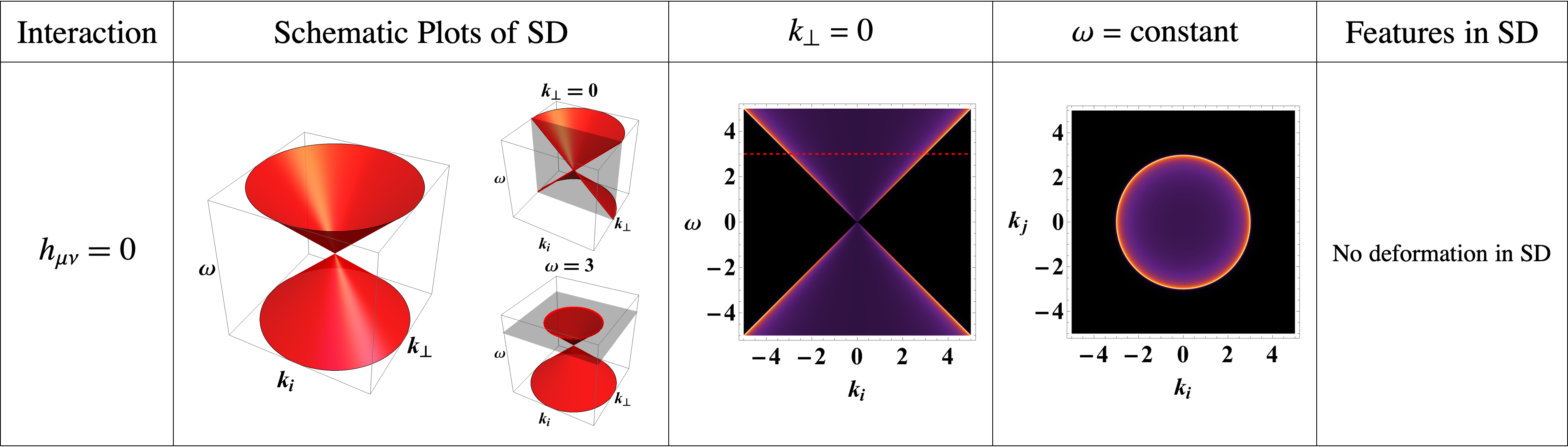
Figure 2: Schematic plots of the spectral density (SD) and its cross-sectional slices for free, massless, and spacelike fermions.

If we turn on each component of the symmetric tensor coupling in (40), we obtain the corresponding retarded Green’s function and the associated spectral density using (41) and (44). We classify the interaction type into $h_{tt}$, $h_{ti}$, $h_{ii}$, and $h_{ij}$ $(i\neq j)$ with $i,j={x,y,z}$. Let $k_{i}$ and $k_{j}$ be three-momentum components associated with the indices of $h_{ti}$, $h_{ii}$, and $h_{ij}$, and $k_{\perp}$ be the remaining three-momentum components. That is, for $h_{tx}$, $k_{i}=k_{x}$ and $k_{\perp}=\{k_{y},k_{z}\}$, whereas for $h_{xy}$, ${k_{i},k_{j}}={k_{x},k_{y}}$ and $k_{\perp}=k_{z}$.

It turns out that for all cases, the Green’s functions of interacting case can be obtained from that of the free fermion by a simple transformation of $(\omega,k_{i})$. We tabulated the result in the table 2.

Int.	Trace of analytic retarded Green’s function	Transformation
$h_{tt}$	$$\mathrm{Tr}G_{R}=\dfrac{2\omega}{\sqrt{\dfrac{|\boldsymbol{k}|^{2}}{(1-\varphi_{tt})^{2}}-\omega^{2}}}$$ (45)	$\begin{gathered}\boldsymbol{k}\to\dfrac{\boldsymbol{k}}{1-\varphi_{tt}}\\ \text{or}\\ \omega\to(1-\varphi_{tt})\omega\end{gathered}$
$h_{ti}$	$$\mathrm{Tr}G_{R}=\dfrac{2(\omega-\varphi_{ti}k_{i})}{\sqrt{\begin{pmatrix}\omega&k_{i}\end{pmatrix}\begin{pmatrix}-1+\varphi_{ti}^{2}&2\varphi_{ti}\\ 2\varphi_{ti}&1-\varphi_{ti}^{2}\end{pmatrix}\begin{pmatrix}\omega\\ k_{i}\end{pmatrix}+|\boldsymbol{k}_{\perp}|^{2}}}$$ (46)	$\begin{pmatrix}\omega\\ k_{i}\end{pmatrix}\to\begin{pmatrix}1&-\varphi_{ti}\\ \varphi_{t}&1\end{pmatrix}\begin{pmatrix}\omega\\ k_{i}\end{pmatrix}$
$h_{ii}$	$$\mathrm{Tr}G_{R}=\dfrac{2\omega}{\sqrt{(1+\varphi_{ii})^{2}k_{i}^{2}+|\boldsymbol{k}_{\perp}|^{2}-\omega^{2}}}$$ (47)	$k_{i}\to(1+\varphi_{ii})k_{i}$
$h_{ij}$	$$\mathrm{Tr}G_{R}=\dfrac{2\omega}{\sqrt{\begin{pmatrix}k_{i}&k_{j}\end{pmatrix}\begin{pmatrix}1+\varphi_{ij}^{2}&2\varphi_{ij}\\ 2\varphi_{ij}&1+\varphi_{ij}^{2}\end{pmatrix}\begin{pmatrix}k_{i}\\ k_{j}\end{pmatrix}+k_{\perp}^{2}-\omega^{2}}}$$ (48)	$\begin{gathered}\begin{pmatrix}k_{i}\\ k_{j}\end{pmatrix}\to R_{\frac{\pi}{4}}^{T}S_{\varphi}R_{\frac{\pi}{4}}\begin{pmatrix}k_{i}\\ k_{j}\end{pmatrix}\\ \begin{cases}R_{\frac{\pi}{4}}:\text{rotation by $\pi/4$}\\ S_{\varphi}=\mathrm{diag}(1-\varphi_{ij},1+\varphi_{ij})\end{cases}\end{gathered}$

Table 2: Traces of the analytic retarded Green’s function and the corresponding momentum transformations for one-flavor spinors under each interaction type (Int.) of symmetric tensor couplings.

Note that all $\mathrm{Tr}G_{R}$ have a branch-cut singularity. By taking the imaginary part of $\mathrm{Tr}G_{R}$ with $\omega\to\omega+i\epsilon$ ($\epsilon>0$), we classify four types of SD in the figure 3 based on their behavior.

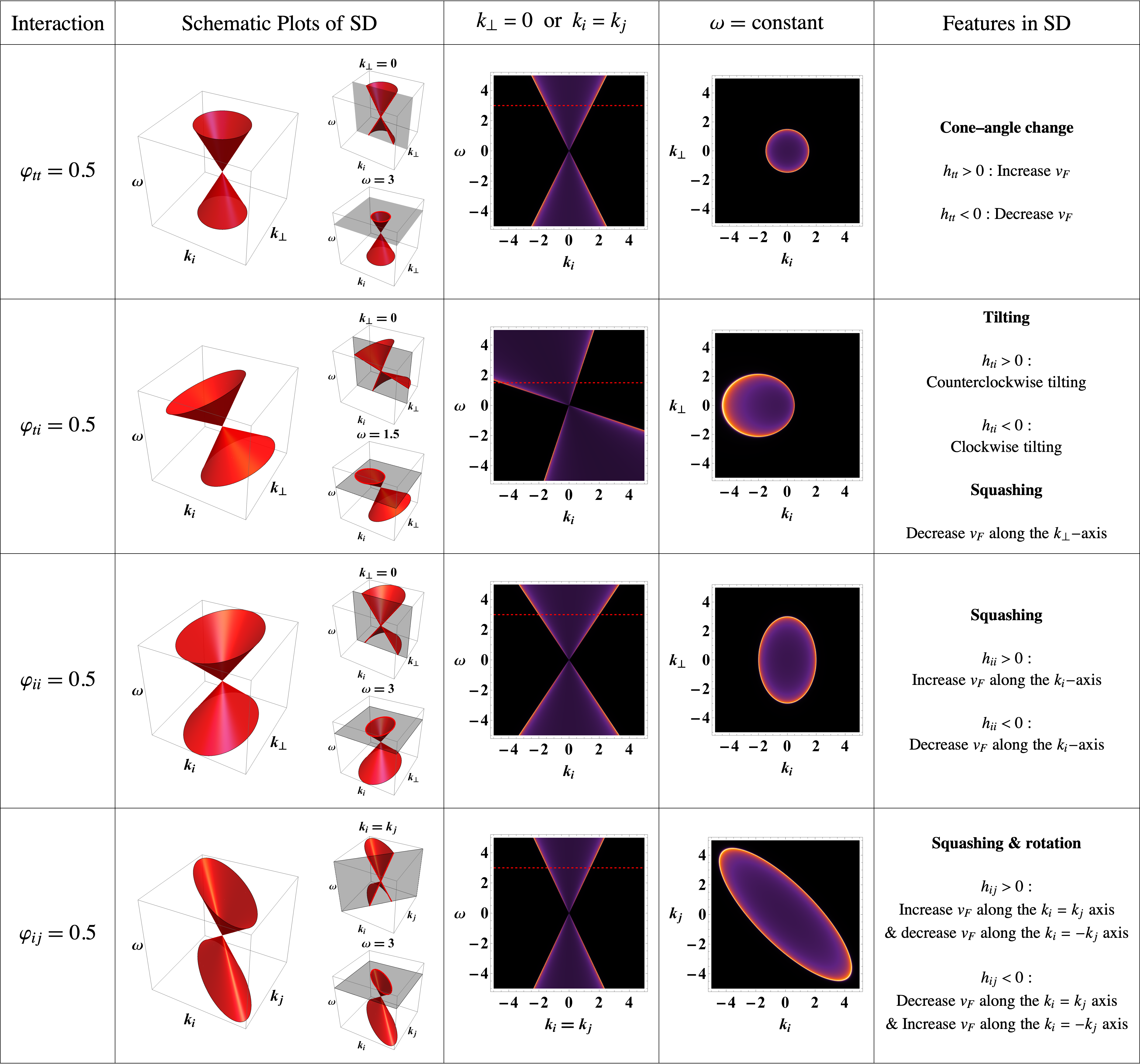
Figure 3: Classification of the spectral density (SD) for massless one-flavor fermions under each type of symmetric tensor coupling. Schematic plots of the SD with $\varphi_{\mu\nu}=0.5$ and their cross-sectional slices (gray planes and red dotted lines) are shown.

In figure 3, the Fermi velocity, $v_{F}$, is defined from the spectral densities as the slope of the SD’s shell in momentum space,

$$v_{F}=\nabla_{\boldsymbol{k}}E(\boldsymbol{k}),$$ (49)

where $E(\boldsymbol{k})$ represents the dispersion relation derived from the pole structure of $\mathrm{Tr}G_{R}$.

As depicted in the table 2 and figure 3, the spectral features associated with each symmetric tensor can be classified into a few categories: cone-angle change, tilting, squashing and rotation:

• The $h_{tt}$ component modifies the Fermi velocity uniformly, increasing it when $h_{tt}>0$ and decreasing it when $h_{tt}<0$, leading to cone-angle change on the spectral density.

• The $h_{ti}$ components induce tilting of spectral densities in the $\omega\text{-}k_{i}$ plane, causing a counterclockwise tilting for $h_{ti}>0$ and a clockwise tilting for $h_{ti}<0$, while preserving the $\pi/2$ cone angle in the same plane. Additionally, these components induce squashing effects on the spectral densities along each $k_{\perp}$-axis, resulting in a reduction of the Fermi velocity along that axis. This, in turn, increases the cone angle in the corresponding direction, independent of the sign of $\varphi_{ti}$. Overall, the $h_{ti}$ component induces asymmetry in the spectral density, including both tilting and squashing effects.

• The $h_{ii}$ components either increase ($h_{ii}>0$) or decrease ($h_{ii}<0$) the Fermi velocity along the $k_{i}$-axis, resulting in squashing effects on the spectral densities in the $k_{i}$-direction.

• The $h_{ij}$ components increase the Fermi velocity along the $k_{i}=k_{j}$ axis while decreasing it along the orthogonal axis ($k_{i}=-k_{j}$) when $h_{ij}>0$, and the effect is reversed for $h_{ij}<0$. As shown in the table 2, this coupling can be interpreted as inducing a squashing ($S_{\varphi}$ in the table 2) and rotation $\pi/4$ ($R_{\frac{\pi}{4}}$ in the table 2) effects on the spectral densities.

In summary, symmetric tensor couplings induce cone-angle change, squashing, and tilting effects on the spectral densities.

So far, we have analyzed the Green’s function and spectral densities for one-flavor spinors under symmetric tensor coupling. In the next section, this framework is extended to incorporate two-flavor spinors.

4 Two-flavor cases

In this section, we analyze the cases with two-flavor spinors coupled with symmetric tensor. The Green’s function and spectral densities for two-flavor spinors can be derived directly from those of the one-flavor cases by combining positive and negative coupling in the one-flavor cases. And so is the classification.

4.1 Dirac equation and source identification

For simplicity, we assume the masses of the flavors are identical. The actions for the two-flavor spinors with symmetric tensor coupling is given by

$$S_{\mathrm{bulk}}=i\sum_{i=1}^{2}\int_{\mathcal{M}}d^{5}x\sqrt{-g}\,\bar{\psi}^{(i)}(\overleftrightarrow{\not{D}}-m)\psi^{(i)},$$ (50)

$$S_{\mathrm{int}}=i\int_{\mathcal{M}}d^{5}x\sqrt{-g}\left(\bar{\psi}^{(1)}h_{MN}\Gamma^{(M}D^{N)}\psi^{(2)}+\bar{\psi}^{(2)}h_{MN}\Gamma^{(M}D^{N)}\psi^{(1)}\right),$$ (51)

$$S_{\mathrm{bdy}}=i\sum_{i=1}^{2}\int_{\partial\mathcal{M}}d^{4}x\sqrt{-gg^{rr}}\bar{\psi}^{(i)}\psi^{(i)}.$$ (52)

From the action, the bulk equations of motion for $\psi^{(i)}$ are given by

$$\begin{pmatrix}\not{D}-m&h_{MN}\Gamma^{(M}D^{N)}\\ h_{MN}\Gamma^{(M}D^{N)}&\not{D}-m\end{pmatrix}\begin{pmatrix}\psi^{(1)}\\ \psi^{(2)}\end{pmatrix}=0.$$ (53)

As in the one-flavor case, we adopt the following ansatz for the two-spinor field:

$$\psi^{(i)}=(-gg^{rr})^{-1/4}e^{-i\omega t+ik_{x}x+ik_{y}y+ik_{z}z}\zeta^{(i)}.$$ (54)

To define the source and condensation for two-flavor spinors, we decompose each flavor field as

$$\psi^{(1)}=\begin{pmatrix}\psi^{(1)}_{+}\\ \psi^{(1)}_{-}\end{pmatrix}\quad\text{and}\quad\psi^{(2)}=\begin{pmatrix}\psi^{(2)}_{+}\\ \psi^{(2)}_{-}\end{pmatrix},$$ (55)

where each $\psi_{\pm}^{(i)}$ ($i=1,2$) is a two-component spinor field. From the field decomposition in (54), we decompose $\zeta^{(i)}$ ($i=1,2$) in the same manner as

$$\zeta^{(1)}=\begin{pmatrix}\zeta^{(1)}_{+}\\ \zeta^{(1)}_{-}\end{pmatrix}\quad\text{and}\quad\zeta^{(2)}=\begin{pmatrix}\zeta^{(2)}_{+}\\ \zeta^{(2)}_{-}\end{pmatrix}.$$ (56)

Then, the boundary action (52) can be rewritten as

$$\begin{gathered}S_{\mathrm{bdy}}=i\sum_{i=1}^{2}\int_{\partial\mathcal{M}}d^{4}x\bar{\zeta}^{(i)}\zeta^{(i)}=\sum_{i=1}^{2}\int_{\partial\mathcal{M}}d^{4}x\,{\zeta^{\dagger}_{+}}^{(i)}\zeta_{-}^{(i)}+\mathrm{h.c.}\end{gathered}$$ (57)

When we vary the bulk action with respect to $\psi^{(i)}$ and add the boundary action variation, one can find that the total action variation can be expressed only in terms of the variation of $\zeta^{(1)}_{+}$ and $\zeta^{(2)}_{+}$ if the equations of motion are satisfied. Therefore, for the standard-standard (SS) quantization method, we identify the source and condensation as the boundary quantities of $(\zeta^{(1)}_{+},\zeta^{(2)}_{+})^{T}$ and $(\zeta^{(1)}_{-},\zeta^{(2)}_{-})^{T}$, respectively. For notational clarity, we denote these bulk quantities as

$$\xi^{(S)}\equiv\begin{pmatrix}\zeta^{(1)}_{+}\\ \zeta^{(2)}_{+}\end{pmatrix}\quad\mathrm{and}\quad\xi^{(C)}\equiv\begin{pmatrix}\zeta^{(1)}_{-}\\ \zeta^{(2)}_{-}\end{pmatrix}.$$ (58)

To extract the source and condensation from $\xi^{(S)}$ and $\xi^{(C)}$, we examine the boundary behavior of $\xi^{(S)}$ and $\xi^{(C)}$ by solving the equations of motion in (53). We observe that the leading terms of $\xi^{(S)}$ and $\xi^{(C)}$ are identical to those of the one-flavor case, as expressed in (21). Thus, we use the same notation, $\mathcal{J}$ and $\mathcal{C}$, as in (21) for the source and condensation of two-flavor spinors, respectively. We utilize this identification of source and condensation when defining the retarded Green’s function for two-flavor spinors.

4.2 Green’s function and spectral densities

To define the retarded Green’s function for two-flavor spinors, we employ our previous development for one-flavor spinors in the section 3.2.

Because $\xi^{(S)}$ and $\xi^{(C)}$ has the same form as (21), we adopt the same calculations in (22)–(26) to express $\mathcal{J}$ and $\mathcal{C}$ in terms of $\mathbb{S}_{0}$ and $\mathbb{C}_{0}$. In addition, notice that the effective action can be expressed in the same form as (27) by rewriting the boundary action in terms of $\xi^{(S)}$ and $\xi^{(C)}$. Therefore, we do the same calculations in (27)–(30) to define the Green’s function for two-flavor spinors, denoted as $\mathbb{G}(r)$, which is expressed as

$$\mathbb{G}_{R}=\mathbb{C}_{0}\mathbb{S}_{0}^{-1}.$$ (59)

We find that the Green’s function in this case can be obtained from that of the one-flavor cases in (33) via a similarity transformation, as detailed in Appendix B. The result is given by

$$\mathbb{G}_{R}=\frac{1}{2}\begin{pmatrix}G_{R}(h)+G_{R}(-h)&&G_{R}(h)-G_{R}(-h)\\ G_{R}(h)-G_{R}(-h)&&G_{R}(h)+G_{R}(-h)\end{pmatrix},$$ (60)

where $G_{R}(h)$ is the Green’s function for one-flavor spinors. Notice that we took Standard quantization for both fermion flavors. Now, the traced Green’s function for two-flavor spinors can be expressed in terms of the one-flavor Green’s function:

$$\mathrm{Tr}\mathbb{G}_{R}=\mathrm{Tr}G_{R}(h)+\mathrm{Tr}G_{R}(-h).$$ (61)

Using the table 2 and (61), we get the traced Green’s function for each tensor coupling and we present the result in the table 3.

Int.	Trace of analytic retarded Green’s function
$h_{tt}$	$$\mathrm{Tr}\mathbb{G}_{R}=\dfrac{2\omega}{\sqrt{\dfrac{\boldsymbol{k}^{2}}{(1-\varphi_{tt})^{2}}-\omega^{2}}}+(\varphi_{tt}\,\leftrightarrow\,-\varphi_{tt})$$ (62)
$h_{ti}$	$$\mathrm{Tr}\mathbb{G}_{R}=\dfrac{2(\omega-\varphi_{ti}k_{i})}{\sqrt{\begin{pmatrix}\omega&k_{i}\end{pmatrix}\begin{pmatrix}-1+\varphi_{ti}^{2}&2\varphi_{ti}\\ 2\varphi_{ti}&1-\varphi_{ti}^{2}\end{pmatrix}\begin{pmatrix}\omega\\ k_{i}\end{pmatrix}+|\boldsymbol{k}_{\perp}|^{2}}}+(\varphi_{ti}\,\leftrightarrow\,-\varphi_{ti})$$ (63)
$h_{ii}$	$$\mathrm{Tr}\mathbb{G}_{R}=\dfrac{2\omega}{\sqrt{(1+\varphi_{ii})^{2}k_{i}^{2}+|\boldsymbol{k}_{\perp}|^{2}-\omega^{2}}}+(\varphi_{ii}\,\leftrightarrow\,-\varphi_{ii})$$ (64)
$h_{ij}$	$$\mathrm{Tr}\mathbb{G}_{R}=\dfrac{2\omega}{\sqrt{\begin{pmatrix}k_{i}&k_{j}\end{pmatrix}\begin{pmatrix}1+\varphi_{ij}^{2}&2\varphi_{ij}\\ 2\varphi_{ij}&1+\varphi_{ij}^{2}\end{pmatrix}\begin{pmatrix}k_{i}\\ k_{j}\end{pmatrix}+k_{\perp}^{2}-\omega^{2}}}+(\varphi_{ij}\,\leftrightarrow\,-\varphi_{ij})$$ (65)

Table 3: Traces of the analytic retarded Green’s function for two-flavor spinors under each interaction type (Int.) of symmetric tensor couplings.

We observe the same classification of interaction types as in the one-flavor case discussed in Section 3.3, based on the components $h_{tt}$, $h_{ti}$, $h_{ii}$, and $h_{ij}$. By taking the imaginary part of (61), we obtain the spectral densities in SS-quantization in terms of those for the one-flavor case, such that

$$A(\omega,\boldsymbol{k})=\mathrm{Im}\left(\mathrm{Tr}\mathbb{G}_{R}\right)=\mathrm{Im}\left(\mathrm{Tr}G_{R}(h)\right)+\mathrm{Im}\left(\mathrm{Tr}G_{R}(-h)\right).$$ (66)

Thus, the spectral densities for two-flavor spinors are a combination of those for one-flavor cases with both positive and negative sign of interactions. From this, we get four types of spectral densities presented in the figure 4.

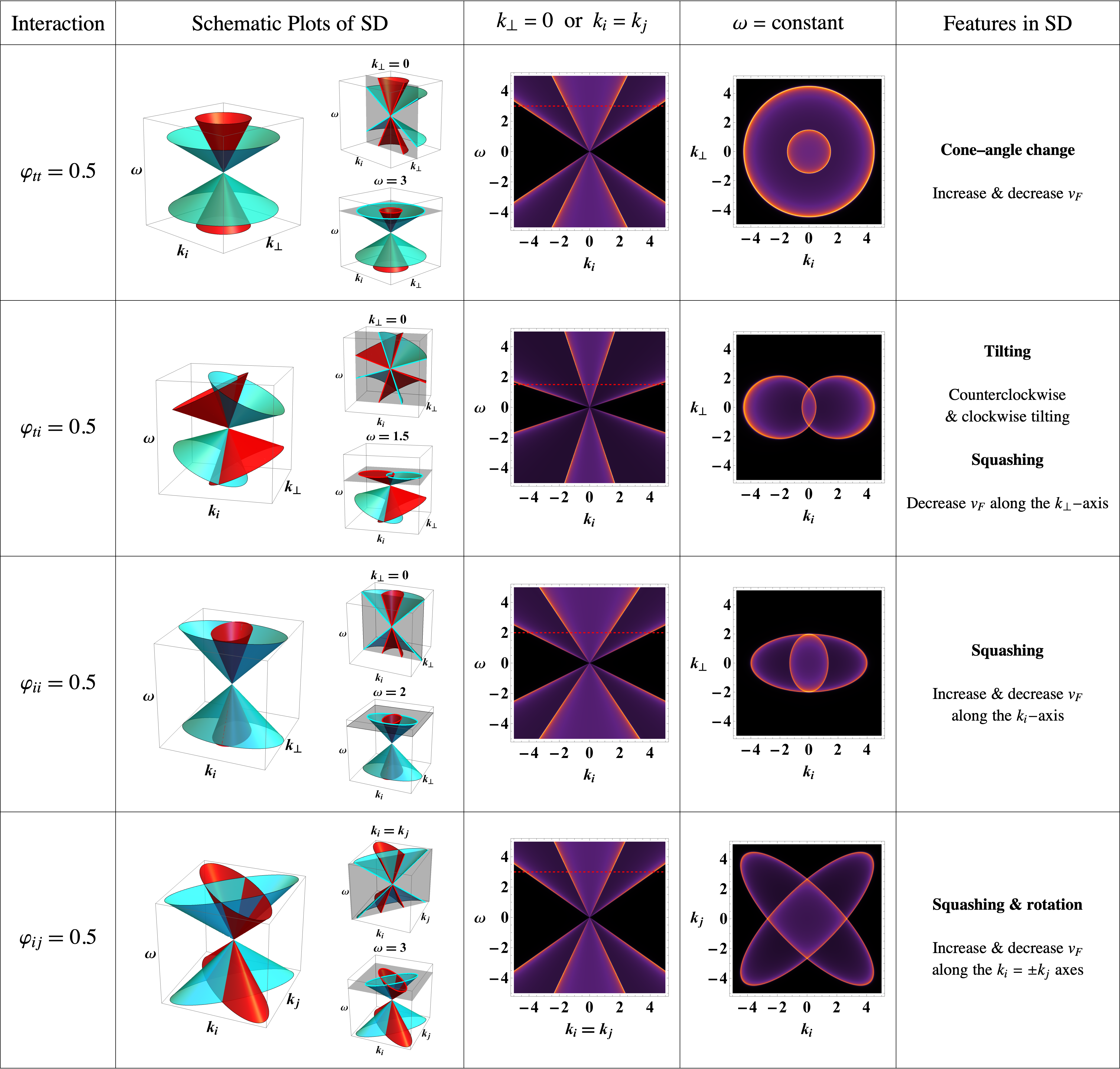
Figure 4: Classification of the spectral density (SD) for massless two-flavor fermions under each type of symmetric-tensor coupling. Schematic plots of the SD with $\varphi_{\mu\nu}=0.5$ and their cross-sectional slices (gray planes and red dotted lines) are shown. Red cones represent contributions from $h_{\mu\nu}>0$, while blue ones represent contributions from $-h_{\mu\nu}$.

From this figure and table 3, we see that the cone-angle change, squashing, and tilting for the one-flavor case can be seen here for both positive and negative coupling.

5 Over-tilted spectral density

In this section, we consider the spectral density with over-tilted cones where upward cone contains the region with negative frequency. One way to get such spectral cone is by introducing both $h_{ti}$ and $h_{ii}$. In this case, the trace of Green’s function is given by

$$\mathrm{Tr}G_{R}=\dfrac{2(\omega-\varphi_{ti}k_{i})}{\sqrt{\begin{pmatrix}\omega&k_{i}\end{pmatrix}\begin{pmatrix}-1+\varphi_{ti}^{2}&\varphi_{ti}(2+\varphi_{ii})\\ \varphi_{ti}(2+\varphi_{ii})&(1+\varphi_{ii})^{2}-\varphi_{ti}^{2}\end{pmatrix}\begin{pmatrix}\omega\\ k_{i}\end{pmatrix}+|\boldsymbol{k}_{\perp}|^{2}}}.$$ (67)

Over-tilted spectral cone can be obtained by imposing appropriate values of $\varphi_{ti}$ and $\varphi_{ii}$ in this formula. For the $\varphi_{ti}=1$ and $\varphi_{ii}=-1$, the result is shown in figure 5.

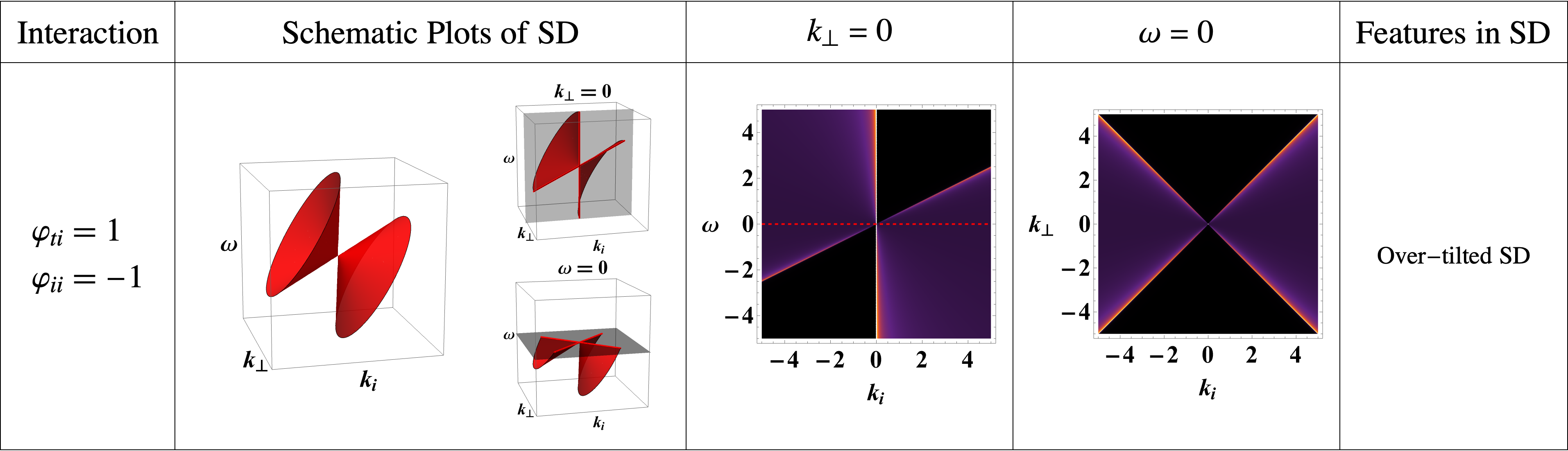
Figure 5: Schematic plots of the spectral density (SD) and its cross-sectional slices (gray planes and red dotted line) for $\varphi_{ti}=1$ and $\varphi_{ii}=-1$.

This spectral density correspond to type-II Dirac cones PhysRevX.9.031010 or Weyl cones at single local Weyl nodes in type-II Weyl semimetals Soluyanov_2015 . Notice that the cone angle in the vertical sectional plane increases due to the squashing effect of $\varphi_{ii}$ along the $k_{i}$-axis. We can produce over-tilted spectral densities by tuning $\varphi_{ti}$ alone, while maintaining their cone angle at $\pi/2$ by turning off $\varphi_{ii}$. Over-tilted spectral cone can be achieved for $\left|\varphi_{ti}\right|>1$ in (46).

5.1 Analytically continued spectral density

One technical issue is in the over tilted cone that there exists a $(\omega,k)$ region where the spectral density is ill-defined with naive value if we use naive infalling boundary condition at the horizon. To resolve this issue, we propose that spectral density should be an analytically continued in that $(\omega,k)$ region which can appear if $\left|\varphi_{ti}\right|>1$. This is the purpose of this subsection.

Within the range $0\leq|\varphi_{ti}|\leq 1$, the tilted spectral density is well-defined, as it remains positive across the entire momentum space. Also, at $\varphi_{ti}=1$, the spectral density exhibits critical tilting, as shown in the figure 6.

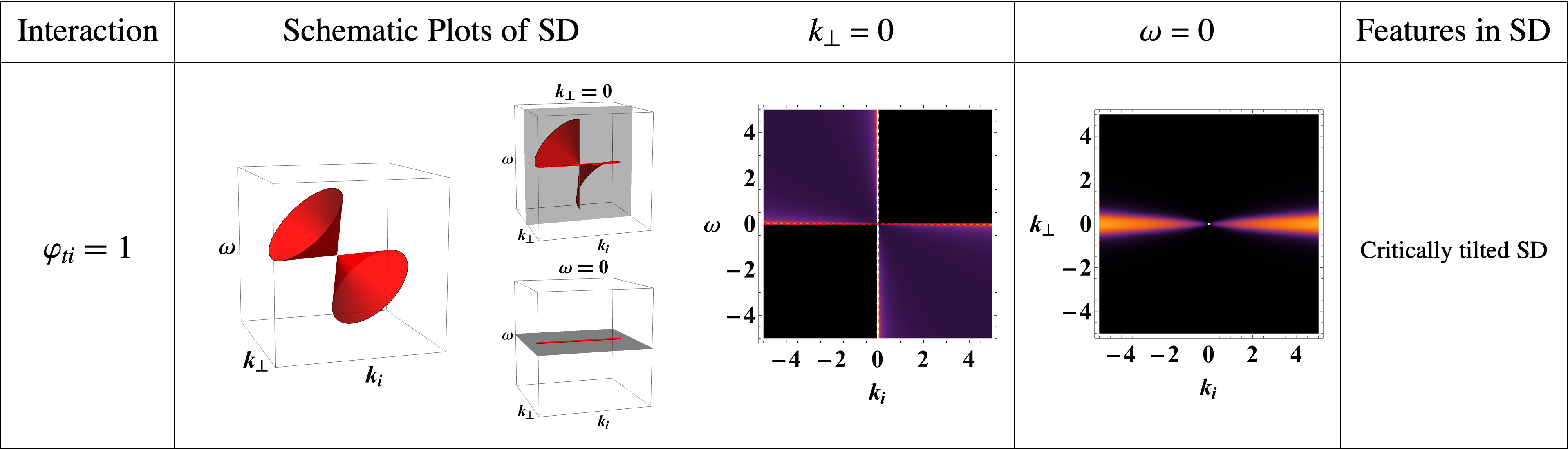
Figure 6: Schematic plots of the spectral density (SD) and its cross-sectional slices (gray planes and red dotted line) for $\varphi_{ti}=1$.

However, for $|\varphi_{ti}|>1$, the spectral densities become ill-defined due to the negative value of $A(\omega,k)$ in the region $\Sigma$ defined by

$$\begin{gathered}\Sigma:=\left\{(\omega,k_{i})\in\mathbb{R}^{2}\,\bigg{|}\,\min\left(A,B\right)\leq\omega\leq\max\left(A,B\right)\right\},\\ \text{where}\quad A=\frac{2\varphi_{ti}}{1-\varphi_{ti}^{2}}k_{i}\quad\text{and}\quad B=\mathrm{sgn}(\varphi_{ti})\left(\dfrac{1+\left|\varphi_{ti}\right|}{1-\left|\varphi_{ti}\right|}\right)k_{i},\end{gathered}$$ (68)

which is plotted in the figure 7.

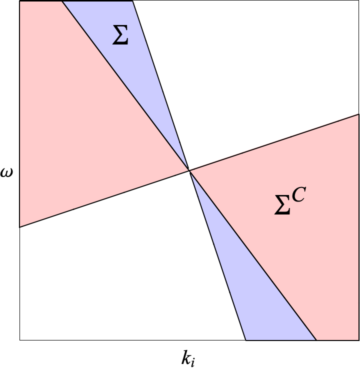
Figure 7: Schematic plot of the spectral density (SD) within the region $(\omega,k_{i})\in\Sigma$ as defined in (68). We impose an alternative near-horizon boundary condition on the Green’s function within the region $\Sigma$ for $|\varphi_{ti}|>1$ and patch it with the complementary region $\Sigma^{C}$, where the spectral densities remain positive.

To ensure the positivity of the spectral densities for $|\varphi_{ti}|>1$, we analytically continue to take the negative value of the square root in (46) in $\Sigma$ for $|\varphi_{ti}|>1$ so that it becomes

$$\mathrm{Tr}G_{R}=\dfrac{-2(\omega-\varphi_{ti}k_{i})}{\sqrt{\begin{pmatrix}\omega&k_{i}\end{pmatrix}\begin{pmatrix}-1+\varphi_{ti}^{2}&2\varphi_{ti}\\ 2\varphi_{ti}&1-\varphi_{ti}^{2}\end{pmatrix}\begin{pmatrix}\omega\\ k_{i}\end{pmatrix}+|\boldsymbol{k}_{\perp}|^{2}}},$$ (69)

$\text{for}\,\,\,(\omega,k_{i})\in\Sigma\,\,\,\mathrm{and}\,\,\,\left|\varphi_{ti}\right|>1.$ This sign change in $\Sigma$ is equivalent to the sign change in the near-horizon boundary condition of $\mathbb{G}(r)$ in $\Sigma$:

$$\mathbb{G}(r\to\infty)=\begin{cases}-i\mathbbm{1}_{2\times 2},&\mathrm{if}\,\,\,(\omega,k_{i})\in\Sigma\,\,\,\mathrm{and}\,\,\,\left|\varphi_{ti}\right|>1,\\ i\mathbbm{1}_{2\times 2},&\mathrm{elsewhere}.\end{cases}$$ (70)

For the explicit derivation, see Appendix D. This means that we should take outgoing condition for spinors if $(\omega,k)\in\Sigma$. This makes perfect sense since $\Sigma$ is the regime where the cone is down ward so that causality should be reversed. By imposing (70) on the flow equation, we find the solution of Green’s function as

$$G_{+}(\omega,\boldsymbol{k}):=\begin{cases}-G_{R}(\omega,\boldsymbol{k}),&\mathrm{if}\,\,\,(\omega,k_{i})\in\Sigma\,\,\,\mathrm{and}\,\,\,\left|\varphi_{ti}\right|>1,\\ G_{R}(\omega,\boldsymbol{k}),&\mathrm{elsewhere}.\end{cases}$$ (71)

Notice that the Green’s function within $\Sigma$ is equivalent to the advanced Green’s function, denoted as $G_{A}(\omega,\boldsymbol{k})$. Consequently, the spectral densities in $\Sigma$ can be identified as the those of the advanced Green’s function, denoted as $A_{A}(\omega,\boldsymbol{k})$. The correct over-tilted spectral densities, which we denote as $A_{+}(\omega,\boldsymbol{k})$, is given by

$$A_{+}(\omega,\boldsymbol{k})=\mathrm{Im}\left(\mathrm{Tr}G_{+}(\omega,\boldsymbol{k})\right):=\begin{cases}\mathrm{Im}\left(\mathrm{Tr}G_{A}(\omega,\boldsymbol{k})\right),&\mathrm{if}\,\,\,(\omega,k_{i})\in\Sigma\,\,\,\mathrm{and}\,\,\,\left|\varphi_{ti}\right|>1,\\ \mathrm{Im}\left(\mathrm{Tr}G_{R}(\omega,\boldsymbol{k})\right),&\mathrm{elsewhere}.\end{cases}$$ (72)

This spectral density is always positive and can be expressed as

$$A_{+}(\omega,\boldsymbol{k})=\left|A_{R}(\omega,\boldsymbol{k})\right|\quad\forall(\omega,\boldsymbol{k})\in\mathbb{R}^{4}\,\,\,\mathrm{and}\,\,\,\forall\varphi_{ti}\in\mathbb{R}.$$ (73)

We draw this for $\varphi_{ti}=2$ in the figure 8.

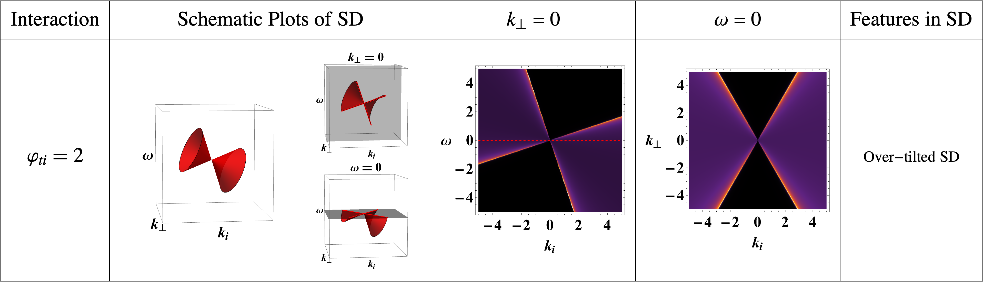
Figure 8: Spectral density $A_{+}(\omega,\boldsymbol{k})$ and its cross-sectional slices (gray planes and red dotted line) for $\varphi_{ti}=2$.

In summary, the well-defined over-tilted spectral densities can be achieved by imposing the correct causal structure for spinors.

5.2 Tilt angle of spectral density

We measure the tilting angle of the spectral density relative to the $\omega$-axis for a given $\varphi_{ti}$ value. The tilting angle is taken to be positive for a positive interaction. See the figure 9(a). By solving the dispersion relation in (73), we derive the tilting angle $\theta$ of the spectral density as a function of $\varphi_{ti}$:

$$\theta=\begin{cases}-\dfrac{\pi}{4}+\arctan\left(\dfrac{1+\varphi_{ti}}{1-\varphi_{ti}}\right),&\text{for}\,\,\,\varphi_{ti}\leq 1,\\[15.0pt] \dfrac{3\pi}{4}+\arctan\left(\dfrac{1+\varphi_{ti}}{1-\varphi_{ti}}\right),&\text{for}\,\,\,\varphi_{ti}>1.\\ \end{cases}$$ (74)

We present this relation in the figure 9(b).

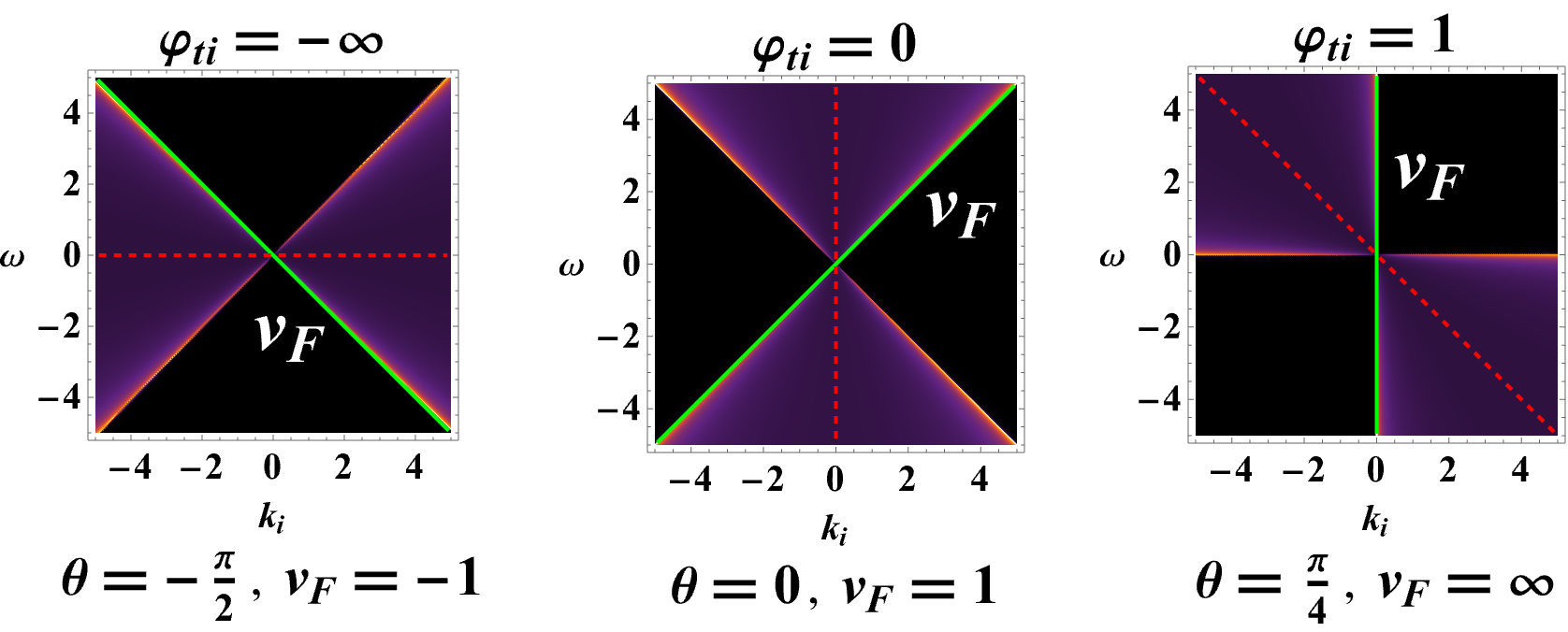
(a) Definition of the counterclockwise tilting angle $\theta$ (red, dashed) and the Fermi velocity (green, solid) within the region where the interaction strength satisfies $\varphi_{ti}\leq 1$.

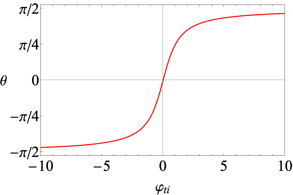
(b) SD’s rotated angle $\theta$ as a function of $\varphi_{ti}$.

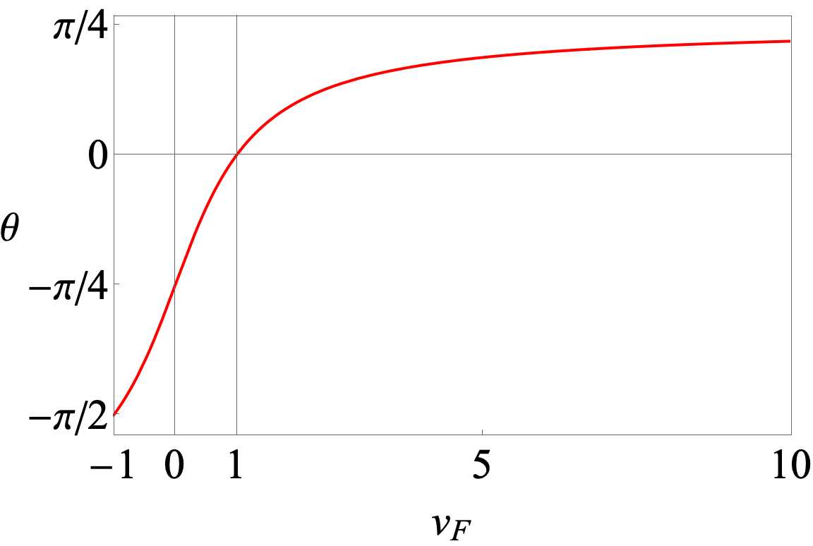
(c) SD’s rotated angle $\theta$ as a function of $v_{F}$.

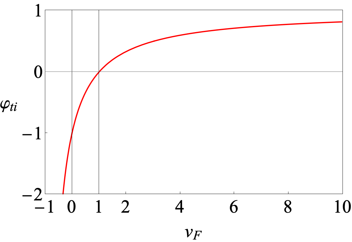
(d) SD’s corresponding $\varphi_{ti}$ as a function of $v_{F}$.

Figure 9: Relations between the Fermi velocity $v_{F}$, the tilting angle $\theta$ of the spectral density, and the coupling strength $\varphi_{ti}$.

From this figure, we see that the tilting angle approaches $\pm\pi/2$ as $\varphi_{ti}$ increases. We can also express the tilting angle $\theta$ in terms of the Fermi velocity $v_{F}$, defined as the positive slope of the spectral cone. See figure 9(a). The tilting angle can also be given as a function of $v_{F}$:

$$\theta=-\dfrac{\pi}{4}+\arctan v_{F}.$$ (75)

We plot this relation in the figure 9(c). As the Fermi velocity increases, the spectral cone asymptotically approaches to the critically tilted case. Finally, we find a relation between $\varphi_{ti}$ and the Fermi velocity by using (74) and (75) such that

$$\varphi_{ti}=\dfrac{v_{F}-1}{v_{F}+1},\quad\text{for}\,\,\,v_{F}\geq-1.$$ (76)

We plot this relation in the figure 9(d).

6 Holography of symmetric tensor coupling vs. Real material

In this section, we explore the application of our holographic mean-field theory with symmetric tensor coupling to condensed matter systems, focusing on the features of spectral densities. To achieve this, we establish the correspondence between the parameters $\varphi_{\mu\nu}$ and their counterparts in condensed matter systems by focusing on the local cone near the Dirac point.

• $h_{tt}$ vs. tuning Fermi velocity
  As shown in the table 2 and figure 3, the $h_{tt}$ component induces cone-angle change, leading to a uniform scaling of the Fermi velocity. The Fermi velocity of Dirac materials such as graphene, can be fine-tuned by applying a uniform electric field, as illustrated in the figure 10(a) quoted from D_az_Fern_ndez_2017 .

  

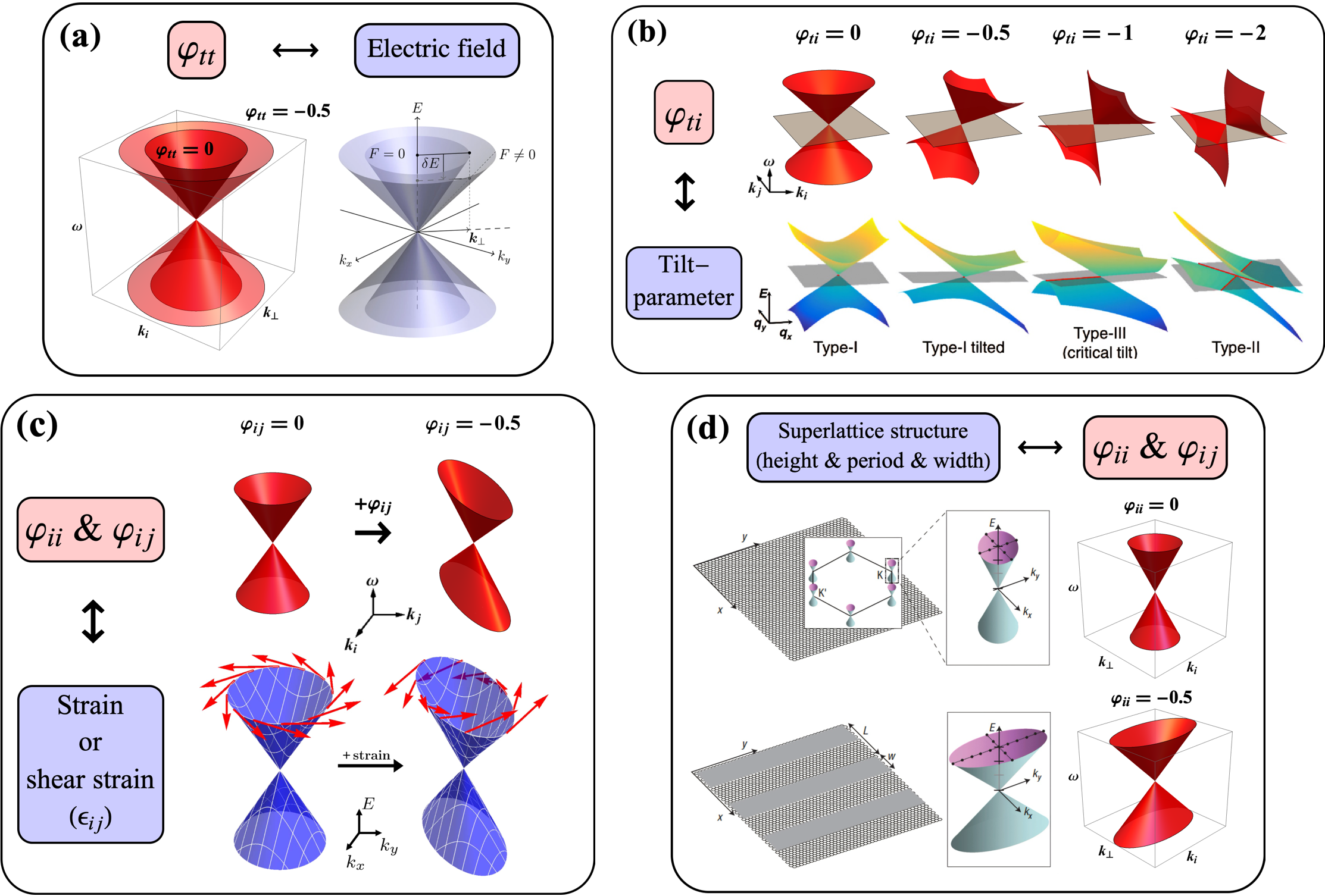
  Figure 10: Holography vs Real material : The red plots represent spectral densities for our holographic model while the blue plots represent those in real matterial system. (a) isotropic tuning of the Fermi velocity induced by a uniform electric field $F$, adapted from D_az_Fern_ndez_2017 ; (b) Tilted Dirac cones, adapted from PhysRevX.9.031010 ; (c) anisotropic Dirac cone on the surface of $\mathrm{Bi}_{2}\mathrm{Se}_{3}$ $(111)$ under strain or shear strain, adapted from Brems_2018 ; (d) squashed Dirac cones in superlattice graphene in periodic potential, adapted from Park_2008 .

  Therefore, the value of $\varphi_{tt}$ serves as the effect of an electric field, enabling isotropic tuning of the Fermi velocity of Dirac cones.

• $h_{tt}$ vs. twist angle
  The dispersion relation in (45) flattens as $\varphi_{tt}\to-\infty$, suggesting a significant suppression of the Fermi velocity. Such locally flat energy spectra are observed in twisted bilayer graphene, where flat bands emerge at the magic angle Lisi_2020 . This similarity gives the possible interpretation of $\varphi_{tt}$ as a parameter analogous to the twist angle in bilayer graphene.

• $h_{ti}$ vs. tilted cones
  $\varphi_{ti}$ serves as a tilt parameter for tilted type-I, II, and III Dirac cones, or Weyl cones at single local Weyl nodes in Weyl semimetals Soluyanov_2015 , as illustrated in the figure 10(b).

• $h_{ii}$ and $h_{ij}$ vs. spin nematic order $Q_{ij}$
  Previously, the spatial symmetric tensor has been used in $d$-wave holographic superconductor. However, our model does not give gap since our model does not have complex field coupled with $U(1)$ gauge field Kim:2013oba ; PhysRevD.109.066004 ; Ghorai:2023wpu . In the spin-nematic action within mean-field theory, the nematic order term PhysRevB.96.235140 parallels the interaction term in (8). So our model has more analogy with the spin-nematic phase characterized by a nematic order parameter $Q_{ij}$, s a quadrupole rank-2 symmetric and traceless tensor PhysRevB.64.195109 ; PhysRevB.96.235140 . Additionally, the spin nematic phase exhibits an anisotropic Fermi surface PhysRevB.96.235140 , which aligns with the squashing of spectral densities under $h_{ii}$ and $h_{ij}$ couplings shown in the figure 3. These parallels suggest that the spatial components $\varphi_{ii}$ and $\varphi_{ij}$ correspond to the $Q_{ij}$ in the spin nematic phase. An analogy between the nematic order and gravitational waves is discussed in PhysRevB.109.L220407 .

• $h_{ii}$ and $h_{ij}$ vs. strain tensor $\epsilon_{ij}$
  Squashing effect on spectral cone can also be found in two-dimensional graphene, where Dirac cones undergo anisotropic deformation due to strain or shear strain PhysRevB.88.085430 ; PhysRevResearch.4.L022027 . Additionally, as shown in the figure 10(c), anisotropic Dirac cones with elliptical equi-energy contours emerge on the $\mathrm{Bi}_{2}\mathrm{Se}_{3}$ $(111)$ surface under applied strain Brems_2018 . These deformations arise via a rank-2 strain tensor $\epsilon_{ij}$ in position or momentum space. It is remarkable that the strain tensor can be quantitatively matched with $\varphi_{ii}$ and $\varphi_{ij}$, as detailed in Appendix C. As a result, the values of $\varphi_{ii}$ and $\varphi_{ij}$ match with the strain tensor $\epsilon_{ij}$, describing Dirac cones that are squashed in the preferred direction.

• $h_{ii}$ and $h_{ij}$ vs. superlattice structure
  In the superlattice graphene, Dirac cones exhibit anisotropic deformation along a preferred direction in momentum space due to a periodically distributed potential Park_2008 , as illustrated in the figure 10(d). As discussed in Park_2008 , the renormalized Fermi velocity depends on the height, period, and width of the periodic potential. Therefore, the structural parameters of the potential can be corresponded to $\varphi_{ii}$ and $\varphi_{ij}$.

The symmetric tensor parameter $\varphi_{\mu\nu}$ can be mactched with measured parameters to reproduce the local energy dispersion of a material. For example, the Dirac cone on the $\mathrm{Bi}_{2}\mathrm{Se}_{3}$ $(221)$ surface exhibits an anisotropic electronic band structure with elliptical equi-energy contours PhysRevB.84.195425 . This anisotropic feature corresponds to the squashed spectral density induced by $h_{ii}$. This correspondence enables us to identify a negative value for $\varphi_{yy}$ to accurately reproduce the elliptical contours reported in PhysRevB.84.195425 . In summary, the values of $\varphi_{\mu\nu}$ can be determined by measuring the Fermi velocities, cone angles, and tilt angles of the local energy dispersion for a given material (See figure 1).

7 Discussion

In this work, we developed a holographic mean-field theory for one- and two-flavor spinors interacting with a rank-2 symmetric tensor field in an $\mathrm{AdS}_{5}$ background. By treating $h_{MN}$ as a order parameter field, we identified three primary effects on fermionic spectral densities: cone-angle change, squashing, and tilting, including over-tilted regimes.

For one-flavor spinors, we derived analytic solutions for the retarded Green’s function and spectral densities in pure $\mathrm{AdS}_{5}$, demonstrating how each boundary component $h_{\mu\nu}$ deforms the shape, cone angle, and Fermi velocity of the spectral densities. Extending this framework, we constructed two-flavor retarded Green’s functions by combining single-flavor solutions with opposite coupling signs. These results enabled a systematic classification of the symmetric tensor field’s roles into cone-angle change, squashing, and tilting effects. We further proposed a method for constructing over-tilted spectral densities ($|\varphi_{ti}|>1$) by patching regions with different causal structures.

In the section 6, we explored physical applications of symmetric tensor couplings, showing a potential phenomenological connection between holography and condensed matter physics. The $\varphi_{tt}$ component governs isotropic Fermi velocity rescaling, observed in Dirac materials under a uniform electric field. Indeed, strong $\varphi_{tt}$ coupling significantly flattens the dispersion, resembling the flat band observed in twisted bilayer graphene at the magic angle. The $\varphi_{ti}$ components acts as a tilt parameter for type-I Dirac or Weyl cones, while over-tilted spectral densities correspond to type-II or type-III Dirac/Weyl semimetals, known for their unique transport properties and causal structures. Spatial components $\varphi_{ii}$ and $\varphi_{ij}$ can be matched to quadrupolar nematic order in spin-nematic systems and strain tensors in strained graphene or $\mathrm{Bi}_{2}\mathrm{Se}_{3}$-class materials. Furthermore, the anisotropic spectral densities from these spatial components align with superlattice graphene under periodic potentials. These connections suggest that symmetric tensor couplings in our holographic model can qualitatively and quantitatively capture the spectral and energy dispersion features of real materials. This framework provides a holographic dictionary for phenomena such as tilted Dirac cones and lattice-driven anisotropic spectral properties.

We want to mention several directions for future research. First, we gave a qualitative mappings between symmetric tensor components and nematic order. And it would be interesing to establish more quantitative correspondence. Second, exploring the topological properties induced by symmetric tensor components, such as Berry curvature will offer promising avenues for further study.

Appendix A Flow equation: derivation and analytical solutions

In this section, we explicitly derive the flow equation in (34) and solve it to obtain the analytic bulk quantity $\mathbb{G}(r)$ in (39).

To set up the flow equation, we substitute the expression in (22) and (23) into the equations of motion in (19) and (20). Then, we get

$$\partial_{r}\mathbb{S}(r)+\mathbb{M}_{1}\mathbb{S}(r)+\mathbb{M}_{2}\mathbb{C}(r)=0,$$ (77)

$$\partial_{r}\mathbb{C}(r)+\mathbb{M}_{3}\mathbb{C}(r)+\mathbb{M}_{4}\mathbb{S}(r)=0,$$ (78)

because ${\bf c}$ is an arbitrary vector in the solution space. When we take a derivative with respect to $r$ on the bulk quantity $\mathbb{G}(r)$ in (31), since $\partial_{r}\mathbb{S}^{-1}=\mathbb{S}(r)^{-1}(\partial_{r}\mathbb{S}(r))\mathbb{S}^{-1}$, we have

$$\partial_{r}\mathbb{G} =\partial_{r}(\mathbb{C}(r)\mathbb{S}(r)^{-1})$$ (79)

$$=(\partial_{r}\mathbb{C}(r))\mathbb{S}(r)^{-1}+\mathbb{C}(r)\partial_{r}\mathbb{S}(r)^{-1}$$

$$=(\partial_{r}\mathbb{C}(r))\mathbb{S}(r)^{-1}-\mathbb{C}(r)\mathbb{S}(r)^{-1}(\partial_{r}\mathbb{S}(r))\mathbb{S}(r)^{-1}.$$

If we substitute (77) and (78) for $\partial_{r}\mathbb{S}(r)$ and $\partial_{r}\mathbb{C}(r)$ in (79), above equation becomes

$$\partial_{r}\mathbb{G}=\mathbb{G}(r)\mathbb{M}_{2}\mathbb{G}(r)+\mathbb{G}(r)\mathbb{M}_{1}-\mathbb{M}_{3}\mathbb{G}(r)-\mathbb{M}_{4}.$$ (80)

By defining $\bar{\mathbb{M}}_{1}\equiv-\mathbb{M}_{1}$ and $\bar{\mathbb{M}}_{2}\equiv-\mathbb{M}_{2}$, we arrive at the desired flow equation presented in (34). For the metric in (12), the four matrices in the flow equation are given by

$$\begin{gathered}\begin{aligned} \bar{\mathbb{M}}_{1}&=\left(\frac{m}{r\sqrt{f}}+\frac{\mathrm{Tr}h/2}{f}+\frac{r^{2}f^{\prime}}{4f^{2}}h_{tt}\right)\mathbbm{1}_{2\times 2}+\frac{r^{2}f^{\prime}}{4f\sqrt{f}}h_{ti}\sigma^{i},\\ \bar{\mathbb{M}}_{2}&=-\dfrac{r^{2}}{f}\left[(g+h)_{t\mu}\bar{k}^{\mu}\right]\mathbbm{1}_{2\times 2}-\dfrac{r^{2}}{\sqrt{f}}(g+h)_{\mu i}\bar{k}^{\mu}\sigma^{i},\\ \mathbb{M}_{3}&=\left(\frac{m}{r\sqrt{f}}-\frac{\mathrm{Tr}h/2}{f}-\frac{r^{2}f^{\prime}}{4f^{2}}h_{tt}\right)\mathbbm{1}_{2\times 2}+\frac{r^{2}f^{\prime}}{4f\sqrt{f}}h_{ti}\sigma^{i},\\ \mathbb{M}_{4}&=-\dfrac{r^{2}}{f}\left[(g+h)_{t\mu}\bar{k}^{\mu}\right]\mathbbm{1}_{2\times 2}+\dfrac{r^{2}}{\sqrt{f}}(g+h)_{\mu i}\bar{k}^{\mu}\sigma^{i},\end{aligned}\\ \text{where}\quad\bar{k}^{\mu}\equiv(\omega/f,\boldsymbol{k}).\end{gathered}$$ (81)

By letting $f=1$ for the pure $\mathrm{AdS}_{5}$ geometry, we can recover the four matrices in (36).

Now, we explicitly show how to derive the solution for $\mathbb{G}(r)$ in (39) using a specific ansatz for it. To solve the flow equation in (37), we set an ansatz of $\mathbb{G}(r)$ as

$$\mathbb{G}(r)=\begin{pmatrix}\mathcal{G}_{11}(r)&\mathcal{G}_{12}(r)\\ \mathcal{G}_{21}(r)&\mathcal{G}_{22}(r)\end{pmatrix}=\begin{pmatrix}a_{11}&a_{12}\\ a_{21}&a_{22}\end{pmatrix}\mathcal{G}(r)=\mathbb{A}\mathcal{G}(r),$$ (82)

where $a_{ij}$ are some constants while $\mathcal{G}(r)$ is a function. We substitute this ansatz into the flow equation (37), so it becomes

$$\mathbb{A}\partial_{r}\mathcal{G}(r)-r^{2}\mathbb{A}\sigma^{\mu}\mathbb{A}(g+h)_{\mu\nu}k^{\nu}\mathcal{G}^{2}(r)+\frac{2m}{r}\mathbb{A}\mathcal{G}(r)-r^{2}\bar{\sigma}^{\mu}(g+h)_{\mu\nu}k^{\nu}=0.$$ (83)

We normalize the coefficients ahead of $\partial_{r}\mathcal{G}$ by dividing $a_{11}$, $a_{12}$, $a_{21}$, and $a_{22}$ on each element of (83). That is, we multiply a matrix ${\scriptsize\begin{pmatrix}1&1\\ 1&1\end{pmatrix}}\mathbb{A}^{-1}$ on (83) so that

$$\begin{pmatrix}1&1\\ 1&1\end{pmatrix}\left(\mathbbm{1}_{2\times 2}\partial_{r}\mathcal{G}(r)-r^{2}\sigma^{\mu}\mathbb{A}(g+h)_{\mu\nu}k^{\nu}\mathcal{G}^{2}(r)+\frac{2m}{r}\mathcal{G}(r)-r^{2}\mathbb{A}^{-1}\bar{\sigma}^{\mu}(g+h)_{\mu\nu}k^{\nu}\right)=0.$$ (84)

Then, we get four differential equations with different coefficients ahead of $\mathcal{G}^{2}(r)$ and the constant terms in (84). We demand that these coefficients have to be same each other for a unique solution of $\mathcal{G}(r)$. Therefore, we impose

$$\sigma^{\mu}\mathbb{A}(g+h)_{\mu\nu}k^{\nu}=c_{1}\mathbbm{1}_{2\times 2}\quad\text{and}\quad\mathbb{A}^{-1}\bar{\sigma}^{\mu}(g+h)_{\mu\nu}k^{\nu}=c_{2}\mathbbm{1}_{2\times 2},$$ (85)

where $c_{1}$ and $c_{2}$ are some constants. By solving these two relations simultaneously with respect to $c_{1}$, $c_{2}$, $a_{12}$, $a_{21}$, and $a_{22}$, we represent $a_{12}$, $a_{21}$, $a_{22}$ in terms of $a_{11}$ as

$$\begin{gathered}a_{12}=-\frac{(\eta+\varphi)_{x\mu}k^{\mu}-i(\eta+\varphi)_{y\nu}k^{\nu}}{(\eta+\varphi)_{t\mu}k^{\mu}-(\eta+\varphi)_{z\mu}k^{\mu}}a_{11},\quad a_{21}=-\frac{(\eta+\varphi)_{x\mu}k^{\mu}+i(\eta+\varphi)_{y\nu}k^{\nu}}{(\eta+\varphi)_{t\mu}k^{\mu}-(\eta+\varphi)_{z\mu}k^{\mu}}a_{11},\\ a_{22}=\frac{(\eta+\varphi)_{t\mu}k^{\mu}+(\eta+\varphi)_{z\nu}k^{\nu}}{(\eta+\varphi)_{t\mu}k^{\mu}-(\eta+\varphi)_{z\mu}k^{\mu}}a_{11}.\end{gathered}$$ (86)

Or, we rewrite these relations in the matrix representation as

$$\begin{pmatrix}a_{11}&a_{12}\\ a_{21}&a_{22}\end{pmatrix}=\frac{\bar{\sigma}^{\mu}(\eta+\varphi)_{\mu\nu}k^{\nu}}{[(\eta+\varphi)_{t\rho}-(\eta+\varphi)_{z\rho}]k^{\rho}}a_{11}.$$ (87)

By substituting this relation into (82), we find

$$\mathbb{G}(r)=\begin{pmatrix}\mathcal{G}_{11}(r)&\mathcal{G}_{12}(r)\\ \mathcal{G}_{21}(r)&\mathcal{G}_{22}(r)\end{pmatrix}=\frac{1}{a_{11}}\begin{pmatrix}a_{11}&a_{12}\\ a_{21}&a_{22}\end{pmatrix}\mathcal{G}_{11}(r)=\frac{\bar{\sigma}^{\mu}(\eta+\varphi)_{\mu\nu}k^{\nu}}{[(\eta+\varphi)_{t\rho}-(\eta+\varphi)_{z\rho}]k^{\rho}}\mathcal{G}_{11}(r)$$ (88)

Therefore, once we solve $\mathcal{G}_{11}(r)$, we solve $\mathbb{G}(r)$ as well. By putting (88) into (37), we get four identical flow equations in the form of

$$\begin{gathered}\partial_{r}\mathcal{G}_{11}(r)+\frac{|(g+h)_{\mu\nu}k^{\nu}|^{2}}{(g+h)_{t\rho}k^{\rho}}r^{2}\mathcal{G}_{11}(r)^{2}+\frac{2m}{r}\mathcal{G}_{11}(r)-r^{2}(g+h)_{t\sigma}k^{\sigma}=0,\\ \text{where}\quad|(g+h)_{\mu\nu}k^{\nu}|^{2}=g^{\mu\nu}(g+h)_{\mu\rho}k^{\rho}(g+h)_{\nu\sigma}k^{\sigma}.\end{gathered}$$ (89)

Also, from (38) and (82), the near-horizon boundary condition for $\mathcal{G}_{11}(r)$ is given by

$$\mathcal{G}_{11}(r\to\infty)=i.$$ (90)

We obtain $\mathcal{G}_{11}(r)$ by solving (89) with the condition (90), then substitute this solution into (88) to obtain $\mathbb{G}(r)$. For spacelike spinors, this solution is given by (39).

Appendix B Derivation of correlator for two-flavor spinors

In this section, we show how to derive the retarded Green’s function for two-flavor spinors in (60).

We begin with the bulk and interaction actions in (50) and (51):

$$\begin{gathered}S_{\mathrm{bulk}}+S_{\mathrm{int}}=i\int_{\mathcal{M}}d^{5}x\sqrt{-g}\begin{pmatrix}\bar{\psi}^{(1)}&\bar{\psi}^{(2)}\end{pmatrix}\begin{pmatrix}\overleftrightarrow{\not{D}}-m&h_{MN}\Gamma^{(M}D^{N)}\\[5.0pt] h_{MN}\Gamma^{(M}D^{N)}&\overleftrightarrow{\not{D}}-m\end{pmatrix}\begin{pmatrix}\psi^{(1)}\\ \psi^{(2)}\end{pmatrix}\end{gathered}$$ (91)

Using the field ansatz in (54), we rewrite this action as

$$S_{\mathrm{bulk}}+S_{\mathrm{int}}=i\int_{\mathcal{M}}d^{5}x\begin{pmatrix}\bar{\zeta}^{(1)}&\bar{\zeta}^{(2)}\end{pmatrix}\begin{pmatrix}\overleftrightarrow{\not{D}}-m&h_{MN}\Gamma^{(M}D^{N)}\\[5.0pt] h_{MN}\Gamma^{(M}D^{N)}&\overleftrightarrow{\not{D}}-m\end{pmatrix}\begin{pmatrix}\zeta^{(1)}\\ \zeta^{(2)}\end{pmatrix}.$$ (92)

We diagonalize the interaction term in (92) using a similarity transformation with an $8\times 8$ matrix $\mathbb{U}$, given by

$$\mathbb{U}=\dfrac{1}{\sqrt{2}}\begin{pmatrix}\mathbbm{1}_{4\times 4}&\mathbbm{1}_{4\times 4}\\ \mathbbm{1}_{4\times 4}&-\mathbbm{1}_{4\times 4}\end{pmatrix}\quad\text{so that}\,\,\,\mathbb{U}^{-1}=\mathbb{U}.$$ (93)

The diagonalization results in

$$\begin{gathered}S_{\mathrm{bulk}}+S_{\mathrm{int}}=i\int_{\mathcal{M}}d^{5}x\begin{pmatrix}\bar{\zeta}^{(1)}&\bar{\zeta}^{(2)}\end{pmatrix}\mathbb{U}^{-1}\mathbb{U}\begin{pmatrix}\overleftrightarrow{\not{D}}-m&h_{MN}\Gamma^{(M}D^{N)}\\[5.0pt] h_{MN}\Gamma^{(M}D^{N)}&\overleftrightarrow{\not{D}}-m\end{pmatrix}\mathbb{U}^{-1}\mathbb{U}\begin{pmatrix}\zeta^{(1)}\\ \zeta^{(2)}\end{pmatrix}\\ =i\int_{\mathcal{M}}d^{5}x\begin{pmatrix}\bar{\phi}^{(1)}&\bar{\phi}^{(2)}\end{pmatrix}\begin{pmatrix}\overleftrightarrow{\not{D}}-m+h_{MN}\Gamma^{(M}D^{N)}&0\\ 0&\overleftrightarrow{\not{D}}-m-h_{MN}\Gamma^{(M}D^{N)}\end{pmatrix}\begin{pmatrix}\phi^{(1)}\\ \phi^{(2)}\end{pmatrix},\\ \mathrm{where}\quad(\phi^{(1)},\phi^{(2)})^{T}=(\phi^{(1)}_{+},\phi^{(1)}_{-},\phi^{(2)}_{+},\phi^{(2)}_{-})^{T}=\mathbb{U}(\zeta^{(1)},\zeta^{(2)})^{T}=\mathbb{U}(\zeta^{(1)}_{+},\zeta^{(1)}_{-},\zeta^{(2)}_{+},\zeta^{(2)}_{-})^{T}.\end{gathered}$$ (94)

Notice that the transformed fields $\phi^{(i)}$ ($i=1,2$) can be expressed in terms of $\xi^{(S)}$ and $\xi^{(C)}$ in (58) as

$$\begin{gathered}\begin{pmatrix}\phi^{(1)}_{+}\\ \phi^{(2)}_{+}\end{pmatrix}=\mathcal{U}\begin{pmatrix}\zeta^{(1)}_{+}\\ \zeta^{(2)}_{+}\end{pmatrix}=\mathcal{U}\xi^{(S)}\quad\text{and}\quad\begin{pmatrix}\phi^{(1)}_{-}\\ \phi^{(2)}_{-}\end{pmatrix}=\mathcal{U}\begin{pmatrix}\zeta^{(1)}_{-}\\ \zeta^{(2)}_{-}\end{pmatrix}=\mathcal{U}\xi^{(C)},\\ \mathrm{where}\quad\mathcal{U}=\dfrac{1}{\sqrt{2}}\begin{pmatrix}\mathbbm{1}_{2\times 2}&\mathbbm{1}_{2\times 2}\\ \mathbbm{1}_{2\times 2}&-\mathbbm{1}_{2\times 2}\end{pmatrix}\quad\text{so that}\,\,\,\mathcal{U}^{-1}=\mathcal{U}.\end{gathered}$$ (95)

From (95), the variation with respect to $\xi^{(S)}$ can be identified as the variation of the transformed field $(\phi_{+}^{(1)},\phi_{+}^{(2)})^{T}$. Likewise, the same identification holds for $\xi^{(C)}$ and $(\phi_{-}^{(1)},\phi_{-}^{(2)})^{T}$. Thus, the source for $\phi^{(i)}$ can be expressed in terms of that for $\psi^{(i)}$, and so can the condensation. By observing the boundary behavior of $\phi^{(i)}$, this correspondence is

$$\begin{gathered}\begin{pmatrix}\phi^{(1)}_{+}\\ \phi^{(2)}_{+}\end{pmatrix}\approx r^{m+\mathrm{Tr}\varphi/2}\mathcal{U}\mathcal{J}=r^{m+\mathrm{Tr}\varphi/2}\mathcal{J}_{\phi}\quad\text{and}\quad\begin{pmatrix}\phi^{(1)}_{-}\\ \phi^{(2)}_{-}\end{pmatrix}\approx r^{-m+\mathrm{Tr}\varphi/2}\mathcal{U}\mathcal{C}=r^{-m+\mathrm{Tr}\varphi/2}\mathcal{C}_{\phi},\\ \mathrm{where}\quad\mathcal{J}_{\phi}=\mathcal{U}\mathcal{J}\quad\mathrm{and}\quad\mathcal{C}_{\phi}=\mathcal{U}\mathcal{C}.\end{gathered}$$ (96)

Consequently, we choose $\mathcal{J}_{\phi}$ as the source and $\mathcal{C}_{\phi}$ as the condensation for $\phi^{(i)}$.

Because $\phi^{(1)}$ and $\phi^{(2)}$ are decoupled in $\eqref{eqB.4}$, finding the Green’s function for $\phi^{(i)}$ is more straightforward than for $\psi^{(i)}$. Thus, we first find the Green’s function for $\phi^{(i)}$, denoted as $\mathbb{G}_{\phi}$. We observe that the form of effective action in (57) remains identical for $\zeta^{(i)}$ and $\phi^{(i)}$, such that

$$S_{\mathrm{eff}}=i\sum_{i=1}^{2}\int_{\partial\mathcal{M}}d^{4}x\,\bar{\zeta}^{(i)}\zeta^{(i)}=i\sum_{i=1}^{2}\int_{\partial\mathcal{M}}d^{4}x\,\bar{\phi}^{(i)}\phi^{(i)}.$$ (97)

Therefore, this effective action defines the same form of the retarded Green’s function for $\mathcal{J}$ and $\mathcal{J}_{\phi}$, such that

$$S_{\mathrm{eff}}=\int_{\partial\mathcal{M}}d^{4}x\,\epsilon^{\mathrm{Tr}\varphi}\mathcal{J}^{\dagger}\mathbb{G}_{R}\mathcal{J}+\mathrm{h.c.}=\int_{\partial\mathcal{M}}d^{4}x\,\epsilon^{\mathrm{Tr}\varphi}\mathcal{J}^{\dagger}_{\phi}\mathbb{G}_{\phi}\mathcal{J}_{\phi}+\mathrm{h.c.}$$ (98)

where $\mathbb{G}_{R}$ is given in (59). By applying the transformation of source in (96) to (98), $\mathbb{G}_{\phi}$ can be expressed in terms of $\mathbb{G}_{R}$ as

$$\mathbb{G}_{\phi}=\mathcal{U}\mathbb{G}_{R}\,\mathcal{U}.$$ (99)

On the other hand, $\mathbb{G}_{\phi}$ is derived from the diagonalized action in (94) and is given by

$$\mathbb{G}_{\phi}=\mathrm{diag}\left(G_{R}(h),G_{R}(-h)\right),$$ (100)

where $G_{R}(h)$ is the retarded Green’s function for a one-flavor spinor. By using (99) and (100), we find the retarded Green’s function for $\psi^{(i)}$ in terms of the that for one-flavor spinors as

$$\mathbb{G}_{R} =\mathcal{U}^{-1}\mathbb{G}_{\phi}\,\mathcal{U}^{-1}$$ (101)

$$=\frac{1}{2}\begin{pmatrix}\mathbbm{1}_{2\times 2}&\mathbbm{1}_{2\times 2}\\ \mathbbm{1}_{2\times 2}&-\mathbbm{1}_{2\times 2}\end{pmatrix}\begin{pmatrix}G_{R}(h)&0\\ 0&G_{R}(-h)\end{pmatrix}\begin{pmatrix}\mathbbm{1}_{2\times 2}&\mathbbm{1}_{2\times 2}\\ \mathbbm{1}_{2\times 2}&-\mathbbm{1}_{2\times 2}\end{pmatrix}$$

$$=\frac{1}{2}\begin{pmatrix}G_{R}(h)+G_{R}(-h)&&G_{R}(h)-G_{R}(-h)\\ G_{R}(h)-G_{R}(-h)&&G_{R}(h)+G_{R}(-h)\end{pmatrix},$$

which is our previous result in (60).

Appendix C Holographic tensor coupling vs. Strain tensor

As we explained in the section 6, the spatial components of the symmetric tensor correspond to the strain tensor, observed in strained two-dimensional graphene, for instance. In this section, we quantitatively match the spatial components $\varphi_{ii}$ and $\varphi_{ij}$ with the strain tensor components $\epsilon_{ii}$ and $\epsilon_{ij}$. We follow the explicit construction of the Hamiltonian for strained graphene in PhysRevB.88.085430 and compare its energy dispersion with that of our spectral density. For notational clarity, we denote the indices $a,b=x,y$ for the strain tensor and spatial symmetric tensor components throughout this section.

We introduce a rank-2 symmetric strain tensor $\epsilon_{ab}$ as

$$\epsilon_{ab}=\begin{pmatrix}\epsilon_{xx}&\epsilon_{xy}\\ \epsilon_{xy}&\epsilon_{yy}\end{pmatrix},$$ (102)

which changes the position of an atom as $\boldsymbol{x}\to(\mathbbm{1}_{2\times 2}+\epsilon_{ab})\cdot\boldsymbol{x}$, where $\boldsymbol{x}$ is the two-dimensional position vector. This strain tensor induces distortion of the reciprocal lattice, leading to anisotropic deformation of the Dirac cone. Around the Dirac point, the Hamiltonian model is given byPhysRevB.88.085430

$$H=v_{0}\sigma^{a}(\delta_{ab}+(1-\beta)\epsilon_{ab})q^{b},$$ (103)

where $v_{0}$ is the Fermi velocity for the undeformed Dirac cone, $\sigma^{a}=(\sigma_{1},\sigma_{2})$, $\beta$ is the difference in hopping energy between the deformed and undeformed lattice, and $q^{a}$ is the momentum measured relative to the Dirac points. To compare this model with our spectral densities, we simply let $v_{0}=1$ and $q^{a}=(k_{x},k_{y})$ at the Dirac point. For the hypothetical case with $\beta=0$, the Hamiltonian in (103) reduces to

$$H=v_{0}\sigma^{a}(\delta_{ab}+\epsilon_{ab})q^{b}.$$ (104)

This $\beta=0$ limit simplifies the analysis of lattice distortion effects by isolating them from hopping energy modifications. The eigenvalues $E_{\pm}$ of the Hamiltonian in (104) are

$$E_{\pm}=\pm\sqrt{((1+\epsilon_{xx})^{2}+\epsilon_{xy}^{2})k_{x}^{2}+2\epsilon_{xy}(2+\epsilon_{xx}+\epsilon_{yy})k_{x}k_{y}+((1+\epsilon_{yy})^{2}+\epsilon_{xy}^{2})k_{y}^{2}}.$$ (105)

In our holographic model, the spectral density for $h_{xx}$, $h_{yy}$, and $h_{xy}$ couplings can be derived from (41). For the comparison with the two-dimensional strained graphene, we let $k_{z}=0$ so that the dispersion from the pole structure in $\mathrm{Tr}G_{R}$ is

$$\omega=\pm\sqrt{((1+\varphi_{xx})^{2}+\varphi_{xy}^{2})k_{x}^{2}+2\varphi_{xy}(2+\varphi_{xx}+\varphi_{yy})k_{x}k_{y}+((1+\varphi_{yy})^{2}+\varphi_{xy}^{2})k_{y}^{2}},$$ (106)

which can be exactly compared with the energy dispersion in (105) by letting $\varphi_{ab}\leftrightarrow\epsilon_{ab}$.

If lattice deformation induces a change in hopping energy ($\beta\neq 0$), the identification is given by

$$\varphi_{ab}\,\leftrightarrow\,(1-\beta)\epsilon_{ab},\quad\text{where}\quad a,b=x,y.$$ (107)

In the realistic case with $\beta\approx 3$ PhysRevB.88.085430 , the sign of $\varphi_{ab}$ corresponding to $(1-\beta)\epsilon_{ab}$ is flipped compared to the hypothetical case with $\beta=0$. Physically, the flipping of $\varphi_{ab}$’s sign corresponds to a reversal in the squashing behavior of the spectral densities, consistent with the $\pi/2$ rotation of strain effects observed in graphene PhysRevB.88.085430 under the hopping-energy modifications.

Appendix D Horizon regularity for over-tilted spectral densities

In this section, we derive the near-horizon boundary condition of $\mathbb{G}(r)$ in $\Sigma$, given in (70). For simplicity, we show this for the $h_{tx}$-coupling.

By solving the flow equation for $h_{tx}$-coupling, the solution for $\mathcal{G}_{11}(r)$ in (82) is given by

$$\mathcal{G}_{11}(r)=-\dfrac{\pi(h_{tx}k_{x}-k_{z}-\omega)\left(2e^{im\pi}K_{m+\frac{1}{2}}(br)+(1+ic_{1})I_{m+\frac{1}{2}}(br)\right)}{2b\,e^{im\pi}K_{m-\frac{1}{2}}(br)-\pi b\,(1+ic_{1})I_{m-\frac{1}{2}}(br)},$$ (108)

where $b$ is the square root in (69), given by $|(\eta+\varphi)_{\mu\nu}k^{\nu}|$, and $c_{1}$ is a constant that must be determined from the horizon regularity. The horizon behavior of this solution is

$$\mathcal{G}_{11}(r)\approx\dfrac{(e^{2br}(c_{1}-i)-e^{im\pi}(c_{1}+i))(h_{tx}k_{x}-k_{z}-\omega)}{b\,e^{2br}(c_{1}-i)+b\,e^{im\pi}(c_{1}+i)}.$$ (109)

Notice that the horizon regularity should be applied differently depending on the sign of $b$ because of the factor $e^{2br}$. For $b>0$, we choose $c_{1}=i$, which gives the ordinary boundary condition in (38). On the other hand, for $b<0$, we choose $c_{1}=-i$, which gives

$$\mathbb{G}(r\to\infty)=-i\mathbbm{1}_{2\times 2}\quad\text{for}\,\,\,b<0.$$ (110)

Therefore, a flipped sign of the square root in $\Sigma$ results in a flipped near-horizon boundary condition for $\mathbb{G}(r)$, suggested in (70).

References

- (1) J.M. Maldacena, The Large N limit of superconformal field theories and supergravity, Int.J.Theor.Phys. 38 (1999) 1113 [hep-th/9711200].
- (2) E. Witten, Anti-de Sitter space and holography, Adv. Theor. Math. Phys. 2 (1998) 253 [hep-th/9802150].
- (3) S.A. Hartnoll, Lectures on holographic methods for condensed matter physics, Class. Quant. Grav. 26 (2009) 224002 [0903.3246].
- (4) T. Faulkner, H. Liu, J. McGreevy and D. Vegh, Emergent quantum criticality, Fermi surfaces, and AdS(2), Phys. Rev. D83 (2011) 125002 [0907.2694].
- (5) T. Faulkner, N. Iqbal, H. Liu, J. McGreevy and D. Vegh, From Black Holes to Strange Metals, 1003.1728.
- (6) A. Donos and J.P. Gauntlett, Holographic Q-lattices, JHEP 04 (2014) 040 [1311.3292].
- (7) M. Blake and D. Tong, Universal Resistivity from Holographic Massive Gravity, Phys. Rev. D88 (2013) 106004 [1308.4970].
- (8) A. Donos and J.P. Gauntlett, The thermoelectric properties of inhomogeneous holographic lattices, JHEP 01 (2015) 035 [1409.6875].
- (9) K.-Y. Kim, K.K. Kim, Y. Seo and S.-J. Sin, Coherent/incoherent metal transition in a holographic model, JHEP 1412 (2014) 170 [1409.8346].
- (10) R.A. Davison, K. Schalm and J. Zaanen, Holographic duality and the resistivity of strange metals, Physical Review B 89 (2014) .
- (11) M. Blake and A. Donos, Quantum critical transport and the hall angle in holographic models, Physical Review Letters 114 (2015) .
- (12) S.A. Hartnoll, A. Lucas and S. Sachdev, Holographic quantum matter, 1612.07324.
- (13) X.-H. Ge, Y. Tian, S.-Y. Wu, S.-F. Wu and S.-F. Wu, Linear and quadratic in temperature resistivity from holography, JHEP 11 (2016) 128 [1606.07905].
- (14) A. Donos, J.P. Gauntlett, T. Griffin and V. Ziogas, Incoherent transport for phases that spontaneously break translations, JHEP 04 (2018) 053 [1801.09084].
- (15) S.A. Hartnoll, C.P. Herzog and G.T. Horowitz, Holographic Superconductors, JHEP 12 (2008) 015 [0810.1563].
- (16) S.A. Hartnoll, C.P. Herzog and G.T. Horowitz, Building a Holographic Superconductor, Phys.Rev.Lett. 101 (2008) 031601 [0803.3295].
- (17) S.S. Gubser, Breaking an Abelian gauge symmetry near a black hole horizon, Phys. Rev. D 78 (2008) 065034 [0801.2977].
- (18) T. Faulkner, G.T. Horowitz, J. McGreevy, M.M. Roberts and D. Vegh, Photoemission ’experiments’ on holographic superconductors, JHEP 03 (2010) 121 [0911.3402].
- (19) G.T. Horowitz and M.M. Roberts, Zero temperature limit of holographic superconductors, Journal of High Energy Physics 2009 (2009) 015–015.
- (20) G.T. Horowitz, Introduction to holographic superconductors, in From Gravity to Thermal Gauge Theories: The AdS/CFT Correspondence, p. 313–347, Springer Berlin Heidelberg (2011), DOI.
- (21) K.-Y. Kim and M. Taylor, Holographic d-wave superconductors, JHEP 08 (2013) 112 [1304.6729].
- (22) N. Iqbal and H. Liu, Real-time response in AdS/CFT with application to spinors, Fortsch. Phys. 57 (2009) 367 [0903.2596].
- (23) J.N. Laia and D. Tong, A holographic flat band, Journal of High Energy Physics 2011 (2011) 125.
- (24) T. Faulkner, N. Iqbal, H. Liu, J. McGreevy and D. Vegh, Charge transport by holographic Fermi surfaces, Phys. Rev. D88 (2013) 045016 [1306.6396].
- (25) E. Oh, Y. Seo, T. Yuk and S.-J. Sin, Ginzberg-Landau-Wilson theory for Flat band, Fermi-arc and surface states of strongly correlated systems, 2007.12188.
- (26) S. Sukrakarn, T. Yuk and S.-J. Sin, Mean field theory for strongly coupled systems: Holographic approach, JHEP 06 (2024) 100 [2311.01897].
- (27) T. Yuk and S.-J. Sin, Flow equation and fermion gap in the holographic superconductors, JHEP 02 (2023) 121 [2208.03132].
- (28) D. Ghorai, T. Yuk and S.-J. Sin, Fermi arc in p-wave holographic superconductors, JHEP 10 (2023) 003 [2304.14650].
- (29) D. Ghorai, T. Yuk and S.-J. Sin, Order parameter and spectral function in -wave holographic superconductors, Phys. Rev. D 109 (2024) 066004.
- (30) H. Im et al., Observation of Kondo condensation in a degenerately doped silicon metal, Nature Phys. 19 (2023) 676 [2301.09047].
- (31) Y.-K. Han, D. Ghorai, T. Yuk and S.-J. Sin, Mean field theory and holographic kondo lattice, 2407.01978.
- (32) V. Oganesyan, S.A. Kivelson and E. Fradkin, Quantum theory of a nematic fermi fluid, Phys. Rev. B 64 (2001) 195109.
- (33) R. Lundgren, H. Yerzhakov and J. Maciejko, Nematic order on the surface of a three-dimensional topological insulator, Phys. Rev. B 96 (2017) 235140.
- (34) L. Chojnacki, R. Pohle, H. Yan, Y. Akagi and N. Shannon, Gravitational wave analogs in spin nematics and cold atoms, Phys. Rev. B 109 (2024) L220407.
- (35) A. Díaz-Fernández, L. Chico, J.W. González and F. Domínguez-Adame, Tuning the fermi velocity in dirac materials with an electric field, Scientific Reports 7 (2017) .
- (36) S. Lisi, X. Lu, T. Benschop, T.A. de Jong, P. Stepanov, J.R. Duran et al., Observation of flat bands in twisted bilayer graphene, Nature Physics 17 (2020) 189–193.
- (37) M. Milićević, G. Montambaux, T. Ozawa, O. Jamadi, B. Real, I. Sagnes et al., Type-iii and tilted dirac cones emerging from flat bands in photonic orbital graphene, Phys. Rev. X 9 (2019) 031010.
- (38) A.A. Soluyanov, D. Gresch, Z. Wang, Q. Wu, M. Troyer, X. Dai et al., Type-ii weyl semimetals, Nature 527 (2015) 495–498.
- (39) G.E. Volovik, Black hole and hawking radiation by type-ii weyl fermions, JETP Letters 104 (2016) 645–648.
- (40) G.E. Volovik, Type-ii weyl semimetal versus gravastar, JETP Letters 114 (2021) 236–242.
- (41) V. Könye, C. Morice, D. Chernyavsky, A.G. Moghaddam, J. van den Brink and J. van Wezel, Horizon physics of quasi-one-dimensional tilted weyl cones on a lattice, Phys. Rev. Res. 4 (2022) 033237.
- (42) S.A. Jafari, Electric field assisted amplification of magnetic fields in tilted dirac cone systems, Phys. Rev. B 100 (2019) 045144.
- (43) J.-W. Seo, T. Yuk, S. Sukrakarn and S.-J. Sin, Tilted dirac cone in holographic material (to appear), .
- (44) M. Oliva-Leyva and G.G. Naumis, Understanding electron behavior in strained graphene as a reciprocal space distortion, Phys. Rev. B 88 (2013) 085430.
- (45) A. Parhizkar and V. Galitski, Strained bilayer graphene, emergent energy scales, and moiré gravity, Phys. Rev. Res. 4 (2022) L022027.
- (46) M.R. Brems, J. Paaske, A.M. Lunde and M. Willatzen, Symmetry analysis of strain, electric and magnetic fields in the bi2se3-class of topological insulators, New Journal of Physics 20 (2018) 053041.
- (47) C.-Y. Moon, J. Han, H. Lee and H.J. Choi, Low-velocity anisotropic dirac fermions on the side surface of topological insulators, Phys. Rev. B 84 (2011) 195425.
- (48) C.-H. Park, L. Yang, Y.-W. Son, M.L. Cohen and S.G. Louie, Anisotropic behaviours of massless dirac fermions in graphene under periodic potentials, Nature Physics 4 (2008) 213–217.
- (49) M.I. Katsnelson, The electronic structure of ideal graphene, in The Physics of Graphene, p. 1–23, Cambridge University Press (2020).
- (50) N. Iqbal and H. Liu, Universality of the hydrodynamic limit in ads/cft and the membrane paradigm, Phys. Rev. D 79 (2009) 025023.