I3S: Importance Sampling Subspace Selection for Low-Rank Optimization in LLM Pretraining

Abstract

Low-rank optimization has emerged as a promising approach to enabling memory-efficient training of large language models (LLMs). Existing low-rank optimization methods typically project gradients onto a low-rank subspace, reducing the memory cost of storing optimizer states. A key challenge in these methods is identifying suitable subspaces to ensure an effective optimization trajectory. Most existing approaches select the dominant subspace to preserve gradient information, as this intuitively provides the best approximation. However, we find that in practice, the dominant subspace stops changing during pretraining, thereby constraining weight updates to similar subspaces.

In this paper, we propose importance sampling subspace selection (I3S) for low-rank optimization, which theoretically offers a comparable convergence rate to the dominant subspace approach. Empirically, we demonstrate that I3S significantly outperforms previous methods in LLM pretraining tasks.

1 Introduction

Large language models (LLMs), pretrained on next-token prediction tasks, achieve human-level text generation capabilities and exhibit zero-shot transferability to various downstream tasks [4]. They are also fine-tuned or aligned with human preferences to be expert in downstream tasks [51, 40]. Over the past few years, there has been rapid progress in LLM development, characterized by consistent growth in the number of trainable parameters and the scale of datasets [1, 26, 10, 2]. The parameter count in language models has increased from 100 million [42] to over a hundred billion [9]. However, despite their enhanced expressiveness, such large models demand extensive GPU memory for pretraining [39]. Thus, a critical question arises:

How can we improve the memory efficiency of LLM pretraining?

In LLM pretraining, Adam is commonly used as the optimizer due to its superior optimization performance. However, a key limitation of Adam is its memory requirement, as it necessitates storing two optimizer states, each consuming as much memory as the model itself. This poses a significant challenge, given the substantial memory demands of the model’s parameters. To address this issue, researchers have explored low-rank optimization, where gradients are projected onto a low-rank subspace to reduce the memory consumption of optimizer states. These states are then projected back to their original size when updating the weights. For example, GaLore [62] and Q-GaLore [57] project gradients onto subspaces defined by the leading singular vectors corresponding to the largest singular values, a technique referred to as the dominant subspace. FLora [20] and GoLore [22], on the other hand, utilize unbiased random low-rank projections for gradients, employing the Johnson–Lindenstrauss transform. Grass [38] introduces sparse low-rank projections, which further reduce the gradient memory footprint as well as the computation and communication costs compared to dense low-rank projections. Lastly, Fira [5] builds on GaLore by fully leveraging the error in gradient low-rank approximation to achieve improved performance.

These methods are powerful because: 1)the gradients of LLMs during pretraining exhibit an intrinsic low-rank structure, making them well-suited for compression using low-rank approximation, and 2) low-rank approximation can be applied not only to Adam but also to other optimizers that use state information. For instance, Adafactor [45] employs rank-1 factorization on the second moment in Adam to reduce the memory required for storing the second moment. Adam-mini [54] eliminates over 99% of the effective learning rate in the second moment of Adam while achieving performance on par with—or even better than—Adam. Additionally, [11] and [29] propose low-precision optimizers with 8-bit and 4-bit optimizer states. Low-rank optimization integrates seamlessly with these Adam variants, further highlighting its importance and underscoring why it deserves significant attention.

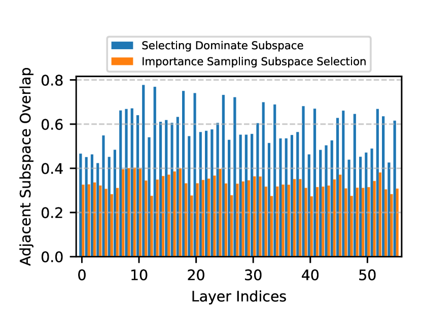
Figure 1: Adjacent subspace overlap of low-rank optimizer using difference subspace selection methods. Importance sampling subspace selection can lower the overlap between adjacent subspaces, thus it enables better exploration in more different subspaces in optimization trajectory.

A central question in low-rank optimization is how to maintain the performance of pretrained LLMs while using memory-efficient optimizers, as compared to full-rank optimization. One common paradigm in existing low-rank optimization methods is to update weights within the dominant subspace for a certain number of iterations and periodically update this dominant subspace. Nonetheless, the dominant subspaces of gradients in many layers stabilize almost completely after the early stages of pretraining [57]. Consequently, the weight updates during different periods predominantly remain within the same low-rank subspace, resulting in cumulative weight updates that struggle to achieve high rank. This limitation significantly hampers the language modeling capabilities of pretrained LLMs. Thus, it is natural to ask:

Is it possible to overcome the low-rank bottleneck of existing low-rank optimization methods without introducing additional overhead?

In this paper, we provide a positive answer to this question. We propose a novel method for subspace selection in low-rank optimization by introducing an appropriate degree of randomness in the selection process. In summary, the contributions of this study are as follows:

• We observe that highly similar adjacent subspaces in existing low-rank optimization methods diminish the diversity of weight updates, degrading the performance of pretrained LLMs.

• To address the low-rank bottleneck in existing low-rank optimization methods, we propose a novel subspace selection method called importance sampling subspace selection (I3S). This method enables low-rank optimizers to explore a broader range of subspaces in the optimization trajectory. Specifically, the low-rank subspace is spanned by $r$ singular vectors sampled from $m$ singular vectors for a gradient $G\in\mathbb{R}^{m\times n}$. Figure 1 illustrates how I3S reduces the overlap between adjacent subspaces during LLM pretraining.

• I3S can be integrated with various low-rank optimization methods, such as GaLore and Fira. It is robust to second-moment factorization and low-precision optimizer state storage. On pretraining tasks for the LLaMA model at different sizes, I3S consistently outperforms dominant subspace selection and reduces the performance gap between low-rank optimizers and full-rank Adam by up to 46.05%.

• From a theoretical aspect, analyzing I3S’s convergence is challenging, because the analysis of weighted sampling without replacement is unwieldy. Therefore, we make a mathematically tractable version of I3S called hybrid subspace selection. We prove that hybrid subspace selection achieves a similar convergence rate as GoLore [22] (Theorem 3.3 and Theorem 3.4) whereas delivering better empirical results (Figure 6). Furthermore, we find that the tunable parameter $r_{0}\in\mathbb{Z}$ in the hybrid subspace selection represents the trade-off between theoretical convergence rate and empirical training stability.

2 Preliminaries

In this section, we present the background required for our theoretical analysis and experiments. In our experiments (Section 4), we apply I3S to two low-rank optimization methods, GaLore and Fira, both of which can be combined with stateful optimizers (e.g., Adam, Adafactor, and Adam-mini).

To ensure clarity, the update rules for GaLore-Adam and Fira-Adam are briefly explained here. For more detailed explanations, please refer to the original papers [62, 5]. In presenting these methods, we show the update rules for the weights of a single layer in the neural network. We assume that the gradient at the $t$-th iteration is a matrix $G^{(t)}\in\mathbb{R}^{m\times n}$. Without loss of generality, we assume that $m<n$ and use $r$ to represent the rank of the low-rank subspace.

2.1 Update Rules of GaLore-Adam

GaLore-Adam [62] requires storing an orthogonal matrix $P^{(t)}\in\mathbb{R}^{m\times r}$ that satisfies $(P^{(t)})^{T}P^{(t)}=I_{r}$, which is updated after a certain number of iterations. Similar to full-rank Adam, GaLore-Adam also requires storing the first moment $M^{(t)}\in\mathbb{R}^{r\times n}$ and the second moment $V^{(t)}\in\mathbb{R}^{r\times n}$ for each layer’s weights, and updating the weights $W^{(t)}$:

$$R^{(t)} =(P^{(t)})^{T}G^{(t)}$$

$$M^{(t)} =\beta_{1}M^{(t-1)}+(1-\beta_{1})R^{(t)}$$

$$V^{(t)} =\beta_{2}V^{(t-1)}+(1-\beta_{2})R^{(t)}\circ R^{(t)}$$

$$N^{(t)} =\alpha P^{(t)}\frac{M^{(t)}}{\sqrt{V^{(t)}}+\xi}$$ (1)

$$x^{(t)} =x^{(t-1)}-\eta\cdot N^{(t)}.$$

where $\beta_{1}$ and $\beta_{2}$ are two hyperparameters for the online update of $M^{(t)}$ and $V^{(t)}$, the same as in Adam, respectively. $\eta$ denotes the learning rate, and $\xi$ denotes a small positive number for numerical stability.

2.2 Update Rules of Fira-Adam

Similar to GaLore-Adam, Fira also needs to store $M^{(t)}$, $V^{(t)}$, and $P^{(t)}$. The difference is that Fira-Adam additionally utilizes the low-rank approximation residual to update $W_{l}^{(t)}$.

$$S^{(t)} =(I-P^{(t)}(P^{(t)})^{T})G^{(t)}$$

$$x^{(t)} =x^{(t-1)}-\eta\cdot N^{(t)}-\eta\cdot\phi(S^{(t)}).$$

where $S^{(t)}$ represents the low-rank approximation error, $\phi(\cdot)$ represents a scaling function in Fira [5], and $N^{(t)}$ is calculated in the same way as in GaLore-Adam shown above (see Eq. (1)).

3 Method

In this section, we first show the adverse phenomenon of the frozen dominant subspace of mini-batch gradients. Then, to address this problem, we propose I3S for low-rank optimization. Finally, we provide the convergence analysis of low-rank optimization with I3S.

Algorithm 1 Low-rank Optimization with I3S

1: Input: The $l$-th layer weight $x_{l}^{(t)}\in\mathbb{R}^{m_{l}\times n_{l}}$, for all $l\in[N]$. Learning rate $\eta$, scale factor $\alpha$, decay rates $\beta_{1},\beta_{2}$, rank $r$, subspace change frequency $\tau\in\mathbb{Z}_{+}$, small constant for numerical stability $\xi$.

2: Initialize: for all $l\in[N]$ $V_{l}^{(0)},M_{l}^{(0)}\in\mathbb{R}^{r\times n_{l}}\leftarrow 0$

3: for $t=1\to T$ do

4:  for $l=1\to N$ do

5:   Compute the mini-batch gradient: $G_{l}^{(t)}\in\mathbb{R}^{m_{l}\times n_{l}}$

6:   $P_{l}^{(t)}\leftarrow\textsc{I3S}(G_{l}^{(t)},\tau)$ {see Algorithm 2}

7:   $x_{l}^{(t)}\leftarrow$ Run GaLore-Adam or Fira-Adam by $V_{l}^{(t-1)},M_{l}^{(t-1)},x_{l}^{(t)},P_{l}^{(t)},G_{l}^{(t)},\beta_{1},\beta_{2},\xi,\eta,\alpha$ {see Section 2.1 and 2.2 respectively}

8:  end for

9: end for

10: Return $x^{(T)}=(x_{1}^{(T)},x_{2}^{(T)},\cdots,x_{N}^{(T)})$

3.1 Frozen Dominate Subspace of Mini-batch Gradient

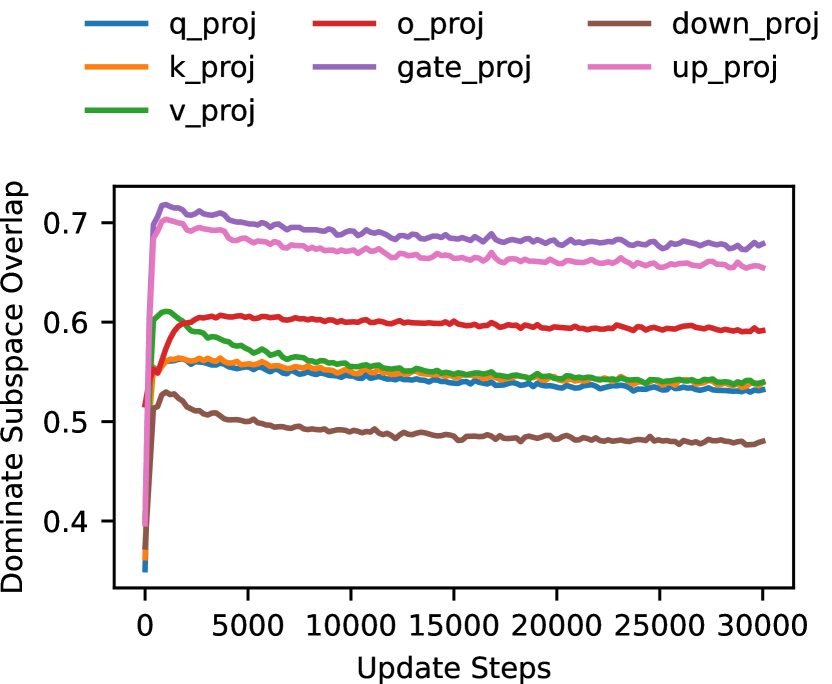
Figure 2: The average mini-batch gradient dominate subspace overlap in different linear layers over 8 blocks in LLaMA-60M model during pretraining. We measure the overlap between adjacent subspaces every 200 iterations.

[57] observes that the cosine similarity between adjacent dominant subspaces approaches 1.0 in some layers after a certain stage of LLM pretraining, indicating that the dominant subspace of the gradient almost stops evolving. We observe a similar phenomenon in our experiment as well. Figure 2 reports the average result of dominant subspace overlap in different layers across all blocks at different iterations. We notice that dominant subspace overlaps are low in all layers at the early stage of pretraining, but they increase drastically as pretraining progresses, eventually becoming stable at different levels. Among all layers, gate_proj and up_proj exhibit the highest subspace overlaps. Intuitively, a high overlap between adjacent subspaces is harmful for low-rank optimization. Considering an extreme case, when the overlap reaches 1.0, the low-rank optimizer can only change the weights within a fixed low-rank subspace. However, when the low-rank subspace shifts significantly over time, the overall weight update—formed by summing updates from various low-rank subspaces—can overcome the constraints of the low-rank bottleneck. For readability, we refer to this phenomenon as the frozen dominant subspace.

3.2 I3S: Importance Sampling Subspace Selection

Algorithm 2 I3S: Importance sampling subspace selection

1: Input: The mini-batch gradient at the iteration $t$, $G_{l}^{(t)}\in\mathbb{R}^{m\times n_{l}}$, where $l\in[N]$ denotes the layer. Subspace change frequency $\tau\in\mathbb{Z}_{+}$.

2: if $t\bmod\tau=0$ then

3:  $U_{l}^{(t)},S_{l}^{(t)},V_{l}^{(t)}\leftarrow\text{SVD}(G_{l}^{(t)})$

4:  $\mathcal{I}\leftarrow\textsc{Sample}([m],\mathrm{num}=r,\mathrm{weight}=S_{l}^{(t)})$

5:  $\mathcal{I}\leftarrow\textsc{Sort}(\mathcal{I})$

6:  $P_{l}^{(t)}\leftarrow U_{l}^{(t)}[:,\mathcal{I}]$

7: else

8:  $P_{l}^{(t)}\leftarrow P_{l}^{(t-1)}$ {Reuse the previous projector}

9: end if

10: Return $P_{l}^{(t)}$

To overcome the problem of the frozen dominate subspace problem, we propose I3S to construct low-rank subspace. Low-rank optimization with I3S is given in Algorithm 1. It can be seen that I3S does not change the overall structure of the original low-rank optimization algorithm but is a plug-and-play substitute for dominant subspace selection. Algorithm 2 gives the procedure of I3S. Line 4 denotes the weighted sampling without replacement. More precisely, each of the $m$ left singular vectors is equipped with a weight $\omega_{i}\in(0,1)$ proportional to its corresponding singular value $S_{i}$,

$$\omega_{i}=\frac{S_{i}}{\sum_{j=1}^{m}S_{j}}.$$

For an index set sample $\mathcal{I}=\left(I_{1},\cdots,I_{r}\right)$, the sampling probability can be written as

$$\mathbb{P}\left\{\left(I_{1},\cdots,I_{r}\right)=\left(i_{1},\cdots,i_{r}\right)\right\}$$

$$=\prod_{k=1}^{r}\frac{\omega_{i_{k}}}{1-\omega_{i_{1}}-\cdots-\omega_{i_{k-1}}}$$

Line 5 sorts the sampled indices in ascending order so that the newly updated subspace basis vectors can align with optimizer states well. Line 6 constructs the orthogonal basis of the new subspace.

By using weighted sampling without replacement, we make adjacent subspaces more different and make the optimization trajectory not be trapped in too similar subspaces during training. Another advantage of I3S is that it does not bring extra overhead.

3.3 Provable Convergence Guarantee

Algorithm 3 Hybrid subspace selection

1: Input: The mini-batch gradient at the iteration $t$, $G_{l}^{(t)}\in\mathbb{R}^{m\times n_{l}}$, where $l\in[N]$ denotes the layer. Subspace change frequency $\tau\in\mathbb{Z}_{+}$.

2: if $t\bmod\tau=0$ then

3:  $U_{l}^{(t)},S_{l}^{(t)},V_{l}^{(t)}\leftarrow\text{SVD}(G_{l}^{(t)})$

4:  $P_{l}^{(t)}[:,:r_{0}]\leftarrow U_{l}^{(t)}[:,:r_{0}]$ {Choose the first $r_{0}$ singular vectors deterministically.}

5:  $P_{l}^{(t)}[:,r_{0}:]\leftarrow\textsc{Unif}(U_{l}^{(t)}[:,r_{0}:],r-r_{0})$ {Choose $(r-r_{0})$ ones by uniform sampling from}

6:  $M_{l}^{(t)}\leftarrow(P_{l}^{(t)})^{T}P_{l}^{(t-1)}M_{l}^{(t-1)}$ {apply momentum projection}

7: else

8:  $P_{l}^{(t)}\leftarrow P_{l}^{(t-1)}$ {Reuse the previous projector}

9: end if

10: Return $P_{l}^{(t)}$

[22] points out that choosing the dominant subspace in low-rank optimization, as in GaLore, does not always guarantee convergence to the optimal solution. They propose a random sampling strategy in subspace selection that ensures provable convergence. However, their random sampling subspace does not significantly alleviate the performance gap between GaLore-Adam and full-rank Adam in the pretraining task, as reported in [22]. In contrast, our method shows empirical advantages, which are deferred to Section 4, and the convergence of our method is provided herein.

One tricky problem with our proposed I3S is the intractability of weighted sampling without replacement. Instead, we analyze a hybrid subspace selection method that is similar to the importance sampling we adopt in practice, as shown in Algorithm 3. The hybrid subspace selection involves choosing the first $r_{0}$ leading singular vectors deterministically out of $m$ available ones, and selecting $(r-r_{0})$ singular vectors from $(m-r_{0})$ singular vectors using uniform sampling. In total, the hybrid subspace selection still selects a rank-$r$ subspace. The difference between this approach and choosing the dominant subspace spanned by the $r$ leading singular vectors is that hybrid subspace selection introduces randomness into subspace selection. The difference between the hybrid subspace selection and using a JL-transform matrix, as in [22], is that the basis vectors in the hybrid subspace selection still align with the direction of mini-batch gradients. Empirically, this difference helps alleviate the gap between low-rank optimization and full-rank optimization. We choose this hybrid subspace selection as an alternative to importance sampling in theoretical analysis, but we do not extend it to our empirical experiments.

We treat an LLM as a neural network with $N$ layers, and each layer has a weight matrix, i.e., $x_{l}\in\mathbb{R}^{m\times n_{l}},\forall l\in[N]$. Without loss of generality, we assume that $m\leq n_{l}$. In practice, most LLMs do not have biases for attention blocks and MLP blocks, and low-rank optimization is only applied to the training weight matrix. Therefore, this abstraction is reasonable. Mathematically, our objective function is

$$f:\mathbb{R}^{m\times n_{1}}\times\mathbb{R}^{m\times n_{2}}\times\dots\times\mathbb{R}^{m\times n_{N}}\to\mathbb{R}$$

For all $x\in\mathrm{dom}(f)$, we denote $\nabla_{l}f(x)$ as $\frac{\partial f}{\partial X_{l}}\in\mathbb{R}^{m\times n_{l}}$. Below, we adopt two assumptions from [22] as follows.

Assumption 3.1 ($L$-smoothness).

Let $f:\mathbb{R}^{m\times n_{1}}\times\mathbb{R}^{m\times n_{2}}\times\dots\times\mathbb{R}^{m\times n_{N}}\to\mathbb{R}$ be our objective function. Let $L>0$. We assume $f$ is $L$-smooth, meaning that it satisfies

$$\left\|\nabla_{l}f(x)-\nabla_{l}f(y)\right\|_{F}\leq L\left\|x-y\right\|_{F}$$

for all $l\in[N]$.

Assumption 3.2 (Bounded and Centered Mini-batch Gradient Noise).

Let $\nabla_{l}f(x^{(t)})\in\mathbb{R}^{m\times n_{l}}$ be the gradient of our objective function for the $l$-th layer at the $t$-th iteration, where $t\in\mathbb{Z}_{+}$. Let $G_{l}^{(t)}\in\mathbb{R}^{m\times n_{l}}$ be the mini-batch gradient which is the noisy version of $\nabla_{l}f(x^{(t)})$.

For all $l\in[N]$, we assume there exists a least upper bound $\sigma_{l}^{2}\in\mathbb{R}$ for $\|G_{l}^{(t)}-\nabla_{l}f(x^{(t)})\|_{F}^{2}$, namely

$$\left\|G_{l}^{(t)}-\nabla_{l}f(x^{(t)})\right\|_{F}^{2}\leq\sigma_{l}^{2}$$

and

$$\mathbb{E}\left[G_{l}^{(t)}\right]=\nabla_{l}f(x^{(t)}).$$

Furthermore, we define $\sigma:=\max_{l\in[N]}\sigma_{l}$.

To compare with [22], we analyze low rank momentum stochastic gradient descent (MSGD). And the convergence rate of low rank MSGD with I3S (as in Algorithm 4) is given by the following theorem.

Theorem 3.3 (Convergence of GaLore-MSGD with hybrid subspace selection).

Under Assumption 3.1-3.2, if $T$ is large enough and we choose the following hyperparameters:

$$\beta_{1}=\left(1+\sqrt{\frac{\delta^{1.5}\sigma^{2}T}{L\Delta}}\right)^{-1},$$

$$\tau=\left\lceil\frac{64}{3\delta\beta_{1}}\right\rceil,$$

$$\eta=\left(4L+\sqrt{\frac{80L^{2}}{3\delta\beta_{1}^{2}}}+\sqrt{\frac{80\tau^{2}L^{2}}{3\delta}}+\sqrt{\frac{16\tau L^{2}}{3\beta_{1}}}\right)^{-1},$$

GaLore with hybrid subspace selection converges in a rate as follows:

$$\frac{1}{T}\sum_{t=0}^{T-1}\mathbb{E}\left[\left\|\nabla f(x^{(t)})\right\|_{F}^{2}\right]=\mathcal{O}\left(\frac{L\Delta}{\delta^{2.5}T}+\sqrt{\frac{L\Delta\sigma^{2}}{\delta^{3.5}T}}\right),$$ (2)

where $\Delta=f(x^{(0)})-\inf_{x}f(x)$, and $\delta=\frac{r-r_{0}}{m-r_{0}}$.

Proofs of Theorem 3.3 is deferred to Appendix A. Below, we present the convergence rate of GoLore [22].

Theorem 3.4 (Corollary 3 from [22]).

Under Assumption 3.1-3.2, let every notation be defined as in Theorem 3.3. Let $\underline{\delta}=\frac{r}{m}$.

Then, GoLore using small-batch stochastic gradients and MSGD converges as

$$\frac{1}{T}\sum_{t=0}^{T-1}\mathbb{E}\left[\left\|\nabla f(x^{(t)})\right\|_{F}^{2}\right]=\mathcal{O}\left(\frac{L\Delta}{\underline{\delta}^{2.5}T}+\sqrt{\frac{L\Delta\sigma^{2}}{\underline{\delta}^{3.5}T}}\right),$$

The Comparison Between Our Technique and Prior Work [22].

To directly compare our work with [22], we adopt the same hyperparameters used in their study. When examining the convergence rate, we note that the primary distinction lies in our use of $\delta=\frac{r-r_{0}}{m-r_{0}}$ (Theorem 3.3), whereas [22] uses $\underline{\delta}=\frac{r}{m}$ (Theorem 3.4). $r_{0}$ can be chosen from the range $[0,r)$. 1). When $r_{0}=0$, this hybrid subspace selection is equivalent to uniform sampling, though this brings the best convergence rate in theory, we observe empirically that uniform sampling sometimes leads to loss spiking, which is the least thing we want to see during training, as shown in Figure 5. 2). When $r_{0}>0$, hybrid subspace selection behaves similarly to I3S, which brings stable loss curve during training. This can be seen as a trade-off between theoretical convergence rate and empirical performance. Note that both the convergence rates of hybrid subspace selection and that of GoLore are better than using dominant subspace, which does not have provable convergence guarantee.

4 Experiments

4.1 Experiment Setting

Pre-training on C4 Dataset.

C4 [43], short for Colossal Clean Crawled Corpus, is a large-scale and open-source text data that are widely used in practice for pre-training transformer models, e.g., BERT [41], T5 [53], and GPT-models. C4 is also widely used in memory efficient optimization community to evaluate the performance of memory-efficient optimizer [20, 62, 57, 22]. In our experiment, we pretrain LLaMA models with different sizes on C4 dataset without data repetition over a sufficient amount of data [19].

Architecture and Hyperparameters

We evaluate different optimizers’ performance on Llama with 60 million, 130 million, 350 million, and 1.1 billion parameters. We adopt the same architecture as in [62]. For experiment with GaLore-Adam, Fira-Adam, and GoLore, we adopt the same hyperparameters as provided in their official codebase. For full-rank Adam, we adopt $\beta_{1}=0.9$, $\beta_{2}=0.999$, $lr=0.001$ except for LLaMA-60M model, whose learning rate is set to be 0.0025.

Table 1: Comparison with different version of Adam on pre-training LLaMA models with 60M, 130M, and 350M parameters on C4 dataset. Validation perplexity is reported.

	60M	130M	350M
Full-Rank Adam	27.71	23.27	18.21
GaLore-I3S-Adam	30.47	24.21	19.16
GaLore-Adam	31.50	24.88	19.68
PPL gap reduction	27.17%	41.61%	35.37%
Fira-I3S-Adam	28.12	22.22	17.25
Fira-Adam	28.42	22.37	17.35
PPL gap reduction	42.25%	—	—
GaLore-I3S-Adafactor	30.06	24.09	18.88
GaLore-Adafactor	31.13	24.79	19.45
PPL gap reduction	31.28%	46.05%	45.96%
GaLore-I3S-Adam-mini	31.66	24.87	19.41
GaLore-Adam-mini	32.08	25.46	19.89
PPL gap reduction	9.61%	26.94%	28.57%
GaLore-I3S-Adam (8bit)	30.55	24.67	18.16
GaLore-Adam (8bit)	31.62	25.35	18.63
PPL gap reduction	27.36%	32.69%	—
$r/d_{model}$	128/256	256/768	256/1024
Tokens	1.5B	2.2B	6B

4.2 Efficacy of I3S with different low-rank Adam optimizers

First, we evaluate the efficacy of I3S when combined with various low-rank Adam optimizers. Table 1 demonstrates that I3S consistently outperforms the selection of the dominant subspace. In cases where full-rank Adam achieves the lowest PPL, we also report the percentage reduction in the PPL gap achieved by I3S compared to using the dominant subspace. As shown in Table 1, I3S reduces the PPL gap by up to 46.05%. In scenarios where full-rank Adam does not achieve the lowest PPL, we observe that I3S still improves PPL compared to selecting leading singular vectors. I3S is effective not only with low-rank variants of Adam, such as GaLore-Adam and Fira-Adam, but also with low-rank optimizers that approximate second moments, e.g., GaLore-Adafactor and GaLore-Adam-mini. Results with the 8-bit optimizer highlight the robustness of I3S against low-precision optimizer state storage.

4.3 Scale Up to Llama-1.1B

Table 2: Comparison among full-rank Adam, GaLore-Adam, and Galore-I3S-Adam on pre-training LLaMA-1.1B on C4 dataset. Validation perplexity is reported.

	Full	GaLore-I3S-Adam	GaLore-Adam
1.1B	15.90	15.36	15.47
$r/d_{model}$	512/2048	512/2048	512/2048
Tokens	13.4B	13.4B	13.4B

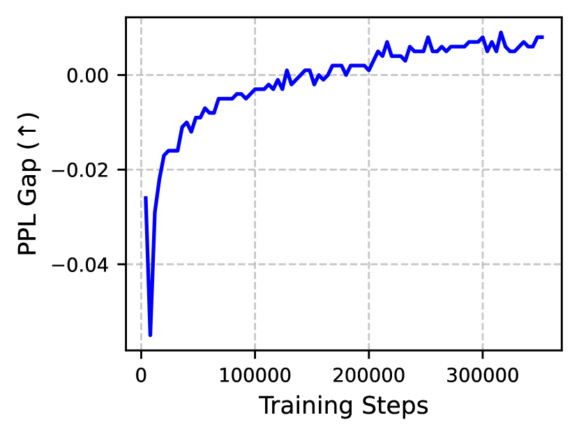
Figure 3: Perplexity gap between GaLore-Adam and GaLore-I3S-Adam during pretaining of LLaMA-1.1B on C4 dataset. PPL gap larger than 0.0 means GaLore-I3S-Adam has a lower PPL than GaLore-Adam.

We also verify the efficacy of I3S on LLaMA-1.1B’s pretraining. Due to limited computational resources, we test it only with GaLore-Adam. Table 2 shows that I3S remains effective on LLaMA-1.1B. Figure 3 illustrates that during the early stage of pretraining, using the dominant subspace performs better than I3S. However, as pretraining progresses, I3S demonstrates its superiority over the dominant subspace. This phenomenon aligns with the insight provided by [22], which suggests that using the dominant subspace during the later stages of pretraining, when noise dominates the gradient, fails to preserve gradient information effectively. While this insight partially explains the advantage of I3S, we provide a more explicit explanation from a new perspective in the next section.

4.4 I3S Enables Higher-rank Update

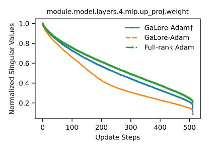
((a))

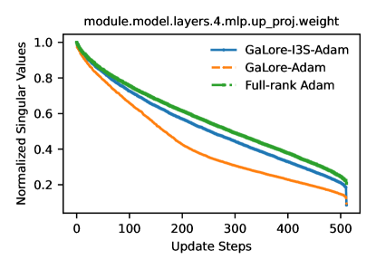
((b))

Figure 4: a). The left figure shows the subspace overlap between adjacent subspaces in GaLore-Adam and GaLore-I3S-Adam during pretraining on the LLaMA-60M model. The definition of subspace overlap is given in Eq. (3). b). The right figure shows normalized singular values of the weight difference between the 28k-step checkpoint and 30k-step checkpoint during pretraining on the LLaMA-60M model.

[57] provides an interesting observation that the similarity between adjacent subspaces in some layers gradually becomes very high during pretraining, we observe a similar phenomenon shown in Figure 2. In Figure 4(a), We observe a similar phenomenon herein in GaLore-Adam, i.e., the overlap between adjacent subspaces becomes large after the early stage of pretraining.

We adopt the metric to measure overlap between two subspaces from [13]. Given two orthonormal matrices $U,V\in\mathbb{R}^{m\times r}$, we have

$$U^{T}U=V^{T}V=I_{r},$$

the overlap between two subspaces spanned by $U$ and $V$ are defined as

$$\text{overlap}(U,V)=\frac{1}{r}\sum_{i=1}^{r}\|U^{T}V_{:,i}\|_{2}^{2},$$ (3)

where $V_{:,i}$ denotes the $i$-th column of V.

We adopt a different measure herein to show that the observation in [57] is not because of the bias of using cosine similarity, but it also exists when using other metrics to measure subspace overlap (or subspace similarity). An interesting fact is that subspace overlap in GaLore-I3S-Adam is much lower, which means GaLore-I3S-Adam tends to explore more different subspaces compared to GaLore-Adam. And as shown in Figure 4(b), because of this broader exploration to different subspaces, the update in GaLore-I3S-Adam has a slower-decaying singular values than that in GaLore-Adam, this indicates a ”higher-rank” update in GaLore-I3S-Adam, and we credit the advantage of I3S over using donminant subspace to it.

4.5 Ablation Study

Different Sampling Distribution and Loss Spiking

Figure 5: Training loss of GaLore-Adam with uniform subspace selection and importance subspace selection on LLaMA-130M’s pretraining. The curve shown in the figure is representative of three seeds.

Because we mentioned in previous context that introducing some randomness into subsapce selection helps to overcome the low-rank bottleneck of update, it is natural to ask what role does the leading singular vectors play in I3S. To answer this, we compare our proposed I3S and uniform singular vector sampling method. We find that I3S helps to avoid loss spiking problem, as shown in Figure 5. Singular vectors corresponding to the first few leading singular values are selected with high probability in importance sampling, and they play an important role in stabilizing training process. Uniform sampling adds too much randomness into subspace selection, which has a negative influence on stable training.

I3S and JL-transform

Figure 6: Evaluation PPL of pretrained LLaMA model with different sizes optimized low-rank Adam with I3S and JL-transform. The numbers of tokens for training are 1.5B, 2.2B, and 6B for 60M, 130M, and 350M model, respectively. Here we run GaLore-I3S-Adam as low-rank Adam with I3S, and GoLore as low-tank Adam with JL-transform.

Here, we demonstrate that I3S outperforms the JL-transform in low-rank optimization. Specifically, we compare GaLore-I3S-Adam with GaLore. The only difference between these two methods is that GaLore-I3S-Adam uses I3S to select the low-rank subspace, whereas GaLore applies the JL-transform to gradients to compress optimizer states. In Section 3.3, we have discussed the difference in convergence rates from a theoretical perspective. Figure 6 illustrates that I3S achieves significantly lower PPL compared to the JL-transform on pretraining tasks.

5 Related Work

Memory Efficient Parametrization.

LoRA [23] can be seen as a memory efficient parametrization of weights in LLMs and is widely used in fine-tuning. LoRA’s bottleneck lies in its low-rank structure and impedes its expressiveness. COLA [52], Delta-LoRA [61], and PLoRA [37] propose to increase the rank and improve the performance of LoRA. ReLoRA [31] and SLTrain [21] extend LoRA to pre-training tasks by merging and resetting adapters, and adopting low-rank plus sparse parameterization, respectively. MoRA [24] alleviate the shortcoming of low-rank disadvantage of LoRA by sharing same trainable parameters to achieve higher-rank update.

Memory Efficient Optimizer.

One way to achieve memory-efficient optimization is by using memory-efficient optimizers, which primarily aim to reduce the memory cost of optimizer states in Adam [28]. A series of works [45, 54, 32, 59] factorizes the second moment in Adam. Quantizing optimizer states and storing them in low-precision formats has also proven successful [29, 11]. Another line of work focuses on gradient compression methods. GaLore [62] and Q-GaLore [57] use SVD to apply dense low-rank projections to gradients. FLora [20] and GoLore [22] adopt random projection, while Grass [38] employs sparse low-rank projection to gradients.

Subspace Learning.

Existing studies provide sophisticated analyses of various subspace learning algorithms [7, 27, 25]. [13] claim that gradient descent primarily occurs in the dominant subspace, which is spanned by the top eigenvectors of the Hessian. In contrast, [44] argue that, due to noise in SGD, the alignment between the gradient and the dominant subspace is spurious, and learning does not occur in the dominant subspace but rather in its orthogonal complement, i.e., the bulk subspace. Intuitively, our findings align with those of [44], suggesting that selecting basis vectors based on specific sampling probabilities can enhance the performance of LLMs during pre-training.

6 Conclusion

In this study, we propose I3S for low-rank optimization in LLM pretraining. The motivation is to find an effective subspace selection method to overcome the low-rank bottleneck caused by the frozen dominant subspace in low-rank optimization. I3S samples singular vectors of mini-batch gradients with probabilities proportional to their singular values, this enables optimization trajectory to explore more different subspaces. Theoretically, in Theorem 3.3, we show that GaLore-I3S-MSGD achieves the same convergence rate as GoLore-MSGD, which is

$$\mathcal{O}\left(\frac{L\Delta}{\delta^{2.5}T}+\sqrt{\frac{L\Delta\sigma^{2}}{\delta^{3.5}T}}\right).$$

Empirically, we find that I3S improves the language modeling capability of pretrained models compared to using the dominant subspace, as verified by experiments involving I3S and dominant subspace selection with multiple low-rank optimizers. Additionally, we compare I3S with uniform singular vector sampling and the JL-transform used in GoLore [22], demonstrating I3S is better at minimizing the sacrifice in pretrained LLM performance compared to full-rank training.

Appendix

Appendix A Proofs of Lemmas and Theorems in Section 3.3

Algorithm 4 Low-rank MSGD with hybrid subspace selection

1: Input: The $l$-th layer weight $x_{l}^{(t)}\in\mathbb{R}^{m_{l}\times n_{l}}$, for all $l\in[N]$, step size $\eta>0$, hyperparameter for hybrid subspace selection $r_{0}$ and $r$, MSGD decay rate $\beta_{1}$.

2: Initialize: for all $l\in[N]$, $M_{l}^{(0)}=\mathbf{0}_{r_{l}\times n_{l}}$.

3: for $t=1\to T$ do

4:  for $l=1\to N$ do

5:   $G_{l}^{(t)}\leftarrow\nabla_{l}f(x^{(t)})+\varepsilon_{l}^{(t)}$ {get mini-batch gradient $G_{l}^{(t)}\in\mathbb{R}^{m_{l}\times n_{l}}$ using the gradient of the objective function $f$ and noise $\varepsilon_{l}^{(t)}\in\mathbb{R}^{m_{l}\times n_{l}}$.}

6:   if $t\bmod\tau=0$ then

7:    $\underbrace{U_{l}^{(t)}}_{m_{l}\times n_{l}},\underbrace{S_{l}^{(t)}}_{n_{l}\times n_{l}},\underbrace{V_{l}^{(t)}}_{n_{l}\times n_{l}}\leftarrow\text{SVD}(G_{l}^{(t)})$

8:    $P_{l}^{(t)}[:,:r_{0}]\leftarrow\underbrace{U_{l}^{(t)}[:,:r_{0}]}_{m_{l}\times r_{0}}$ {Choose the first $r_{0}$ singular vectors deterministically.}

9:    $P_{l}^{(t)}[:,r_{0}:]\leftarrow\underbrace{\mathsf{Unif}(U_{l}^{(t)}[:,r_{0}:],r-r_{0})}_{m_{l}\times(n_{l}-r_{0})}$ {Choose $(r-r_{0})$ ones by uniform sampling from}

10:    $\underbrace{M_{l}^{(t)}}_{r_{l}\times n_{l}}\leftarrow\underbrace{(P_{l}^{(t)})^{T}}_{r_{l}\times m_{l}}\underbrace{P_{l}^{(t-1)}}_{m_{l}\times r_{l}}\underbrace{M_{l}^{(t-1)}}_{r_{l}\times n_{l}}$ {apply momentum projection}

11:   else

12:    $P_{l}^{(t)}\leftarrow\underbrace{P_{l}^{(t-1)}}_{m_{l}\times r_{l}}$ {Reuse the previous projector}

13:   end if

14:   $\underbrace{R_{l}^{(t)}}_{r_{l}\times n_{l}}\leftarrow\underbrace{(P_{l}^{(t)})^{T}}_{r_{l}\times m_{l}}\underbrace{G_{l}^{(t)}}_{m_{l}\times n_{l}}$ {Project gradient into low-rank subspace}

15:   $\underbrace{M_{l}^{(t)}}_{r_{l}\times n_{l}}\leftarrow\beta_{1}\cdot\underbrace{M_{l}^{(t-1)}}_{r\times n_{l}}+(1-\beta_{1})\cdot\underbrace{R_{l}^{(t)}}_{r_{l}\times n_{l}}$ {Update momentum}

16:   $\underbrace{\tilde{M}_{l}^{(t)}}_{m_{l}\times n_{l}}\leftarrow\underbrace{P_{l}^{(t)}}_{m_{l}\times r_{l}}\underbrace{M_{l}^{(t)}}_{r_{l}\times n_{l}}$ {Project momentum back to full size}

17:   $\underbrace{x_{l}^{(t+1)}}_{m_{l}\times n_{l}}\leftarrow\underbrace{x_{l}^{(t)}}_{m_{l}\times n_{l}}-\eta\cdot\underbrace{\widetilde{M}_{l}^{(t)}}_{m_{l}\times n_{l}}$ {Update weight}

18:  end for

19: end for

Before proceeding to the proof of GaLore-MSGD with Importance Sampling, we need to adopt some important lemmas.

Lemma A.1 (Descent Lemma from [22]).

Under the assumption of L-smooth objective function, for update

$$x^{(t+1)}=x^{(t)}-\eta\widetilde{M}^{(t)},$$

we have

$$f(x^{(t+1)})\leq f(x^{(t)})-\left(\frac{1}{2\eta}-\frac{L}{2}\right)\left\|x^{(t+1)}-x^{(t)}\right\|_{F}^{2}+\frac{\eta}{2}\left\|\widetilde{M}^{(t)}-\nabla f(x^{(t)})\right\|_{F}^{2}-\frac{\eta}{2}\left\|\nabla f(x^{(t)})\right\|_{F}^{2}$$

We adopt similar proof routinue as in [22], first we need a Momentum Contraction Lemma for Sampling Subspace Selection, which is shown as Lemma A.2.

Lemma A.2 (Momentum Contraction).

Let $G_{l}^{(t)}$ be an unbiased estimator of the gradient $\nabla_{l}F(x^{(0)})$ with variance bounded by $\sigma_{l}^{2}$. Define

$$\delta=\frac{r-r_{0}}{m-r_{0}}$$

• Part 1. When $t=0$, we have

  $$\mathbb{E}\left[\left\|\widetilde{M}_{l}^{(0)}-\nabla_{l}f(x^{(0)})\right\|_{F}^{2}\right]\leq\left(1-(2\beta_{1}-\beta_{1}^{2})\frac{r-r_{0}}{m-r_{0}}\right)\mathbb{E}\left[\left\|\nabla_{l}f(x^{(0)})\right\|_{F}^{2}\right]+\beta_{1}^{2}\sigma_{l}^{2}.$$

• Part 2. When $t=k\tau$, $k\in\mathbb{N}$, we have

  $$\mathbb{E}\left[\left\|\widetilde{M}_{l}^{(t)}-\nabla_{l}f(x^{(t)})\right\|_{F}^{2}\right]-(1-(1-\frac{\delta}{4})\beta_{1})\mathbb{E}\left[\left\|\widetilde{M}_{l}^{(t-1)}-\nabla_{l}f(x^{(t-1)})\right\|_{F}^{2}\right]$$ (4)

  $$\leq \frac{2(1-\delta)}{\tau}\sum_{r=0}^{\tau-1}\mathbb{E}\left[\left\|\nabla_{l}f(x^{(k\tau+r)})\right\|_{F}^{2}\right]+\frac{5(1-\beta_{1})}{\beta_{1}\delta}\mathbb{E}\left[\left\|\nabla_{l}f(x^{(t)})-\nabla_{l}f(x^{(t-1)})\right\|_{F}^{2}\right]$$ (5)

  $$~+(\tau-1)(1-\delta)\sum_{r=0}^{\tau-2}\mathbb{E}\left[\left\|\nabla_{l}f(x^{(k\tau+r+1)})-\nabla_{l}f(x^{(k\tau+r)})\right\|\right]+\beta_{1}^{2}\sigma_{l}^{2}$$ (6)

• Part 3. When $t=k\tau+r$, $k\in\mathbb{N}$, $1\leq r\leq\tau-1$,

  $$\mathbb{E}\left[\left\|\widetilde{M}_{l}^{(t)}-\nabla_{l}f(x^{(t)})\right\|_{F}^{2}\right]-(1-(1-\frac{\delta}{4})\beta_{1})\mathbb{E}\left[\left\|\widetilde{M}_{l}^{(t-1)}-\nabla_{l}f(x^{(t-1)})\right\|_{F}^{2}\right]$$

  $$\leq \left(1-\frac{\delta}{2}\right)\beta_{1}\mathbb{E}\left[\left\|\nabla_{l}f(x^{(t)})\right\|_{F}^{2}\right]+\frac{5(1-\beta_{1})}{\beta_{1}\delta}\mathbb{E}\left[\left\|\nabla_{l}f(x^{(t)})-\nabla_{l}f(x^{(t-1)})\right\|_{F}^{2}\right]$$

  $$~+\frac{10r\beta_{1}}{\delta}\sum_{i=1}^{r}\mathbb{E}\left[\left\|\nabla_{l}f(x^{(k\tau+i)})-\nabla_{l}f(x^{(k\tau+i-1)})\right\|_{F}^{2}\right]+\beta_{1}^{2}\sigma_{l}^{2}$$

Proof.

Proof of Part 1.

When $t=0$, we have

$$\mathbb{E}\left[\left\|\widetilde{M}_{l}^{(0)}-\nabla_{l}f(x^{(0)})\right\|_{F}^{2}\right] =\mathbb{E}\left[\left\|\beta_{1}P_{l}^{(0)}\left(P_{l}^{(0)}\right)^{T}\left(G_{l}^{(0)}-\nabla_{l}f(x^{(0)})\right)\right\|_{F}^{2}\right]$$

$$\quad+\mathbb{E}\left[\left\|\left(\beta_{1}P_{l}^{(0)}\left(P_{l}^{(0)}\right)^{T}-I\right)\nabla_{l}f(x^{(0)})\right\|_{F}^{2}\right],$$ (7)

which follows from definition of $\widetilde{M}_{l}^{(0)}$ and the unbiasness of $G_{l}^{(0)}$. For the first term, using Assumption 3.2 we have

$$\mathbb{E}\left[\left\|\beta_{1}P_{l}^{(0)}\left(P_{l}^{(0)}\right)^{T}\left(G_{l}^{(0)}-\nabla_{l}f(x^{(0)})\right)\right\|_{F}^{2}\right]\leq\beta_{1}^{2}\sigma_{l}^{2}$$ (8)

For the second term, we have

$$\mathbb{E}\left[\left\|\left(I-\beta_{1}P_{l}^{(0)}\left(P_{l}^{(0)}\right)^{T}\right)\nabla_{l}f(x^{(0)})\right\|_{F}^{2}\right]$$

$$= \mathbb{E}_{\nabla_{l}f(x^{(0)})}\left[\mathbb{E}_{P_{l}^{(0)}}\left[\left\|\left(I-\beta_{1}P_{l}^{(0)}\left(P_{l}^{(0)}\right)^{T}\right)\nabla_{l}f(x^{(0)})\right\|_{F}^{2}\middle|\nabla_{l}f(x^{(0)})\right]\right]$$

$$= \mathbb{E}_{\nabla_{l}f(x^{(0)})}\left[\mathbb{E}_{P_{l}^{(0)}}\left[\mathrm{tr}\left(\nabla_{l}f(x^{(0)})^{T}\left(I-\beta_{1}P_{l}^{(0)}\left(P_{l}^{(0)}\right)^{T}\right)^{2}\nabla_{l}f(x^{(0)})\right)\middle|\nabla_{l}f(x^{(0)})\right]\right]$$

$$= \mathbb{E}_{\nabla_{l}f(x^{(0)})}\left[\mathrm{tr}\left(\mathbb{E}_{P_{l}^{(t)}}\left[\nabla_{l}f(x^{(0)})^{T}\left(I-\beta_{1}P_{l}^{(0)}\left(P_{l}^{(0)}\right)^{T}\right)^{2}\nabla_{l}f(x^{(0)})\middle|\nabla_{l}f(x^{(0)})\right]\right)\right]$$

$$= \mathbb{E}_{\nabla_{l}f(x^{(0)})}\left[\mathrm{tr}\left(\mathbb{E}_{P_{l}^{(t)}}\left[\sum_{j=r_{0}+1}^{m}\left(1-(2\beta_{1}-\beta_{1}^{2})\mathbf{1}_{\{j\}}\right)\cdot\nabla_{l}f(x^{(t)})^{T}U_{j}U_{j}^{T}\nabla_{l}f(x^{(0)})\middle|\nabla_{l}f(x^{(0)})\right]\right)\right]$$

$$= \mathbb{E}_{\nabla_{l}f(x^{(0)})}\left[\mathrm{tr}\left(\sum_{j=r_{0}+1}^{m}\left(1-(2\beta_{1}-\beta_{1}^{2})\frac{r-r_{0}}{m-r_{0}}\right)\cdot\nabla_{l}f(x^{(0)})^{T}U_{j}U_{j}^{T}\nabla_{l}f(x^{(0)})\right)\right]$$

$$\leq \left(1-(2\beta_{1}-\beta_{1}^{2})\frac{r-r_{0}}{m-r_{0}}\right)\cdot\mathbb{E}_{\nabla_{l}f(x^{(0)})}\left[\mathrm{tr}\left(\sum_{j=1}^{m}\nabla_{l}f(x^{(0)})^{T}U_{j}U_{j}^{T}\nabla_{l}f(x^{(0)})\right)\right]$$

$$= \left(1-(2\beta_{1}-\beta_{1}^{2})\frac{r-r_{0}}{m-r_{0}}\right)\mathbb{E}\left[\left\|\nabla_{l}f(x^{(0)})\right\|_{F}^{2}\right],$$ (9)

where the first step follows from the law of total expectation, the second step follows from $\|A\|_{F}=\sqrt{\mathrm{tr}(A^{T}A)}$, the third step follows from simple algebra, the fourth step follows from the fact that $P_{l}^{(0)}$ is selected by using hybrid subspace sampling method, the sixth step follows from $\mathbb{E}[aX]=a\mathbb{E}[X]$, and the last step follows from $\|A\|_{F}=\sqrt{\mathrm{tr}(A^{T}A)}$.

Combining Eq. (8) and Eq. (A) together, we have

$$\mathbb{E}\left[\left\|\widetilde{M}_{l}^{(0)}-\nabla_{l}f(x^{(0)})\right\|_{F}^{2}\right]\leq\left(1-(2\beta_{1}-\beta_{1}^{2})\frac{r-r_{0}}{m-r_{0}}\right)\mathbb{E}\left[\left\|\nabla_{l}f(x^{(0)})\right\|_{F}^{2}\right]+\beta_{1}^{2}\sigma_{l}^{2}.$$ (10)

Proof of Part 2. The proof of Part 2 is very similar to the proof of Part 2 in Lemma 10 from [22]. The difference is that we do not have

$$\mathbb{E}\left[\left\|P_{l}^{(t)}(P_{l}^{(t)})^{T}\left((1-\beta_{1})\widetilde{M}_{l}^{(t-1)}+\beta_{1}G_{l}^{(t)}-\nabla_{l}f(x^{(t)})\right)\right\|_{F}^{2}\right]$$

$$\leq\delta\cdot\mathbb{E}\left[\left\|\left((1-\beta_{1})\widetilde{M}_{l}^{(t-1)}+\beta_{1}G_{l}^{(t)}-\nabla_{l}f(x^{(t)})\right)\right\|_{F}^{2}\right],$$

but instead we have a slightly looser bound

$$\mathbb{E}\left[\left\|P_{l}^{(t)}(P_{l}^{(t)})^{T}\left((1-\beta_{1})\widetilde{M}_{l}^{(t-1)}+\beta_{1}G_{l}^{(t)}-\nabla_{l}f(x^{(t)})\right)\right\|_{F}^{2}\right]$$

$$\leq\mathbb{E}\left[\left\|\left((1-\beta_{1})\widetilde{M}_{l}^{(t-1)}+\beta_{1}G_{l}^{(t)}-\nabla_{l}f(x^{(t)})\right)\right\|_{F}^{2}\right].$$

Based on this and following the corresponding proof steps in [22], we can get Eq. (4).

Proof of Part 3. The result of Part 3 and the proof in Part 3 is the same as in [22]. ∎

Though our Momentum Contraction result is a little worse than the one in [22], we can still get the same result for Momentum Error Bound, as shown in Lemma A.3.

Lemma A.3 (Momentum Error Bound).

Define

$$\sigma^{2}=\sum_{l\in[N]}\sigma_{l}^{2}$$

Then we have

$$\sum_{t=0}^{K\tau-1}\mathbb{E}\left[\left\|\widetilde{M}^{(t)}-\nabla f(x^{(t)})\right\|_{F}^{2}\right]$$ (11)

$$\leq \left(\frac{5(1-\beta_{1})}{(1-\delta/4)\delta\beta_{1}^{2}}+\frac{5\tau(1-\tau)}{(1-\delta/4)\delta}+\frac{\tau-1}{(1-\delta/4)\beta}\right)L^{2}\sum_{t=0}^{K\tau-2}\mathbb{E}\left[\left\|x^{(t+1)}-x^{(t)}\right\|_{F}^{2}\right]$$ (12)

$$~+\left(\frac{1-\delta/2}{1-\delta/4}+\frac{2}{(1-\delta/4)\beta_{1}}\right)\sum_{t=0}^{K\tau-2}\mathbb{E}\left[\left\|\nabla f(x^{(t)})\right\|_{F}^{2}\right]+\frac{K\tau\beta_{1}\sigma^{2}}{1-\delta/4}$$ (13)

Proof.

The proof is in the similar manner as the proof of momentum error bound in [22]. However, because there is some difference between our momentum contraction result and their momentum contraction result, we show our proof here.

First we apply summation to Eq. • ‣ A.2 as follows:

$$\sum_{t=k\tau+1}^{(k+1)\tau-1}\mathbb{E}\left[\left\|\widetilde{M}_{l}^{(t)}-\nabla_{l}f(x^{(t)})\right\|_{F}^{2}\right]-\left(1-(1-\frac{\delta}{4})\beta_{1}\right)\sum_{t=k\tau+1}^{(k+1)\tau-1}\mathbb{E}\left[\left\|\widetilde{M}_{l}^{(t-1)}-\nabla_{l}f(x^{(t-1)})\right\|_{F}^{2}\right]$$

$$\leq \left(1-\frac{\delta}{2}\right)\beta_{1}\sum_{t=k\tau+1}^{(k+1)\tau-1}\mathbb{E}\left[\left\|\nabla_{l}f(x^{(t)})\right\|_{F}^{2}\right]$$

$$~+\frac{5(1-\beta_{1})}{\beta_{1}\delta}\sum_{t=k\tau+1}^{(k+1)\tau-1}\mathbb{E}\left[\left\|\nabla_{l}f(x^{(t)})-\nabla_{l}f(x^{(t-1)})\right\|_{F}^{2}\right]$$

$$~+\frac{10\beta_{1}}{\delta}\sum_{r=1}^{\tau-1}r\sum_{i=1}^{r}\mathbb{E}\left[\left\|\nabla_{l}f(x^{(k\tau+i)})-\nabla_{l}f(x^{(k\tau+i-1)})\right\|_{F}^{2}\right]$$

$$~+\beta_{1}^{2}\sigma_{l}^{2}(\tau-1)$$

$$\leq \left(1-\frac{\delta}{2}\right)\beta_{1}\sum_{t=k\tau+1}^{(k+1)\tau-1}\mathbb{E}\left[\left\|\nabla_{l}f(x^{(t)})\right\|_{F}^{2}\right]$$

$$~+\left[\frac{5(1-\beta_{1})}{\beta_{1}\delta}+\frac{5\beta_{1}\tau(\tau-1)}{\delta}\right]\sum_{t=k\tau}^{(k+1)\tau-2}\mathbb{E}\left[\left\|\nabla_{l}f(x^{(t+1)})-\nabla_{l}f(x^{(t)})\right\|_{F}^{2}\right]$$

$$~+\beta_{1}^{2}\sigma_{l}^{2}(\tau-1)$$ (14)

Then add Eq. (A) and Eq. (4) together, we have

$$\sum_{t=k\tau}^{(k+1)\tau-1}\mathbb{E}\left[\left\|\widetilde{M}_{l}^{(t)}-\nabla_{l}f(x^{(t)})\right\|_{F}^{2}\right]-\left(1-(1-\frac{\delta}{4})\beta_{1}\right)\sum_{t=k\tau}^{(k+1)\tau-1}\mathbb{E}\left[\left\|\widetilde{M}_{l}^{(t-1)}-\nabla_{l}f(x^{(t-1)})\right\|_{F}^{2}\right]$$

$$\leq \left[\left(1-\frac{\delta}{2}\right)\beta_{1}+\frac{2(1-\delta)}{\tau}\right]\sum_{t=k\tau}^{(k+1)\tau-1}\mathbb{E}\left[\left\|\nabla_{l}f(x^{(t)})\right\|_{F}^{2}\right]$$

$$~+\left[\frac{5(1-\beta_{1})}{\beta_{1}\delta}+\frac{5\beta_{1}\tau(\tau-1)}{\delta}+(\tau-1)(1-\delta)\right]\sum_{t=k\tau}^{(k+1)\tau-2}\mathbb{E}\left[\left\|\nabla_{l}f(x^{(t+1)})-\nabla_{l}f(x^{(t)})\right\|_{F}^{2}\right]$$

$$~+\beta_{1}^{2}\sigma_{l}^{2}\tau$$

Then applying summation over $k$ from 0 to $K$ and summation over all $l\in[N]$ gives us Eq. (11). ∎

Theorem A.4 (Convergence rate of GaLore-MSGD with sampling subspace selection).

Let $\eta>0$ be the learning rate. We define $m:=\min_{l\in[N]}m_{l}$. Let $\delta_{r_{0}}\in(0,1)$ be the relative low-rank approximation error of mini-batch gradient. We choose hyperparameter $\beta_{1}\in(0,1)$ to satisfy that $\widetilde{\delta}_{r_{0}}<1-\beta_{1}$, where

$$\widetilde{\delta}_{r_{0}}:=\max\left\{\left(1-\beta_{1}\right)^{2}\left(1-\frac{r-r_{0}}{m-r_{0}}\right),\delta_{r_{0}}\right\}.$$

and choose learning rate

$$\eta\leq\min\{\frac{1}{2L},\frac{1-\beta_{1}}{\sqrt{2}\beta_{1}L}\}.$$

We define

$$C_{r_{0}}:=(1-\beta_{1})^{2}+(1-\frac{r-r_{0}}{m-r_{0}})+\delta_{r_{0}}$$

and

$$\Delta:= ~\frac{1-\beta_{1}}{1-\beta_{1}-\widetilde{\delta}_{r_{0}}}(\frac{2}{\eta}\mathbb{E}[f(x^{(0)})-f(x^{*})]$$

$$~+\mathbb{E}[\|\widetilde{M}^{(0)}-\nabla f(x^{(0)})\|_{F}^{2}]).$$

Then, we have

$$~\frac{1}{(k+1)\tau}\sum_{t=0}^{(k+1)\tau-1}\mathbb{E}\left[\left\|\nabla f(x^{(t)})\right\|_{F}^{2}\right]$$

$$~\leq\frac{\Delta}{(k+1)\tau}+\frac{C_{r_{0}}}{1-\beta_{1}}\sigma^{2}$$

Proof.

From Lemma A.1, we have

$$f(x^{(t+1)})\leq f(x^{(t)})-\left(\frac{1}{2\eta}-\frac{L}{2}\right)\left\|x^{(t+1)}-x^{(t)}\right\|_{F}^{2}+\frac{\eta}{2}\left\|\widetilde{M}^{(t)}-\nabla f(x^{(t)})\right\|_{F}^{2}-\frac{\eta}{2}\left\|\nabla f(x^{(t)})\right\|_{F}^{2},$$

by simply rearrange different terms, we have

$$\frac{\eta}{2}\left\|\nabla f(x^{(t)})\right\|_{F}^{2}$$

$$\leq f(x^{(t)})-f(x^{(t+1)})-\left(\frac{1}{2\eta}-\frac{L}{2}\right)\left\|x^{(t+1)}-x^{(t)}\right\|_{F}^{2}+\frac{\eta}{2}\left\|\widetilde{M}^{(t)}-\nabla f(x^{(t)})\right\|_{F}^{2}$$

By summing over $t$ from 0 to $T$, we have

$$~\sum_{t=0}^{T}\mathbb{E}[\|\nabla f(x^{(t)})\|_{F}^{2}]$$

$$\leq ~\frac{2}{\eta}(f(x^{(0)})-f(x^{(*)}))-\frac{2}{\eta}(\frac{1}{2\eta}-\frac{L}{2})\sum_{t=0}^{T}\mathbb{E}[\|x^{(t+1)})-x^{(t)})\|_{F}^{2}]+\sum_{t=0}^{T}\mathbb{E}[\|\widetilde{M}^{(t)}-\nabla f(x^{(t)})\|_{F}^{2}]$$

$$\leq ~\frac{2}{\eta}(f(x^{(0)})-f(x^{(*)}))-\frac{2}{\eta}(\frac{1}{2\eta}-\frac{L}{2})\sum_{t=0}^{T}\mathbb{E}[\|x^{(t+1)})-x^{(t)})\|_{F}^{2}]$$

$$+ ~\sum_{t=1}^{T}\frac{\beta_{1}^{2}}{(1-\beta_{1})^{2}}\mathbb{E}[\|\nabla_{l}f(x^{(t)})-\nabla_{l}f(x^{(t-1)})\|_{F}^{2}]$$

$$+ ~\sum_{t=1}^{T}(1-\beta_{1})(1-\frac{r-r_{0}}{m-r_{0}})\mathbb{E}[\|\nabla_{l}f(x^{(t)})\|_{F}^{2}]$$

$$+ ~T\cdot(1-\beta_{1})\sigma_{l}^{2}$$

$$+ ~\frac{1}{1-\beta_{1}}\mathbb{E}[\|\widetilde{M}_{l}^{(0)}-\nabla_{l}f(x^{(0)})\|_{F}^{2}]$$

$$\leq ~\frac{2}{\eta}(f(x^{(0)})-f(x^{(*)}))-\frac{2}{\eta}(\frac{1}{2\eta}-\frac{L}{2})\sum_{t=0}^{T}\mathbb{E}[\|x^{(t+1)})-x^{(t)})\|_{F}^{2}]$$

$$+ ~\sum_{t=1}^{T}\frac{L^{2}\beta_{1}^{2}}{(1-\beta_{1})^{2}}\mathbb{E}[\|x^{(t)}-x^{(t-1)}\|_{F}^{2}]$$

$$+ ~\sum_{t=1}^{T}(1-\beta_{1})(1-\frac{r-r_{0}}{m-r_{0}})\mathbb{E}[\|\nabla_{l}f(x^{(t)})\|_{F}^{2}]$$

$$+ ~T\cdot(1-\beta_{1})\sigma_{l}^{2}$$

$$+ ~\frac{1}{1-\beta_{1}}\mathbb{E}[\|\widetilde{M}_{l}^{(0)}-\nabla_{l}f(x^{(0)})\|_{F}^{2}]$$

$$\leq ~\frac{2}{\eta}(f(x^{(0)})-f(x^{(*)}))$$

$$+ ~(\frac{L^{2}\beta_{1}^{2}}{(1-\beta_{1})^{2}}-\frac{2}{\eta}(\frac{1}{2\eta}-\frac{L}{2}))\sum_{t=0}^{T}\mathbb{E}[\|x^{(t+1)})-x^{(t)})\|_{F}^{2}]$$

$$+ ~\sum_{t=1}^{T}(1-\beta_{1})(1-\frac{r-r_{0}}{m-r_{0}})\mathbb{E}[\|\nabla_{l}f(x^{(t)})\|_{F}^{2}]$$

$$+ ~T\cdot(1-\beta_{1})\sigma_{l}^{2}$$

$$+ ~\frac{1}{1-\beta_{1}}\mathbb{E}[\|\widetilde{M}_{l}^{(0)}-\nabla_{l}f(x^{(0)})\|_{F}^{2}]$$

Then by reordering terms on both sides and using proper learning rate $\eta$, we have

$$\frac{1}{T}\mathbb{E}\left[\left\|\nabla f(x^{(t)})\right\|_{F}^{2}\right]$$

$$\leq\frac{1}{1-(1-\beta_{1})(1-\frac{r-r_{0}}{m-r_{0}})}\cdot\frac{2}{\eta}\cdot\frac{\Delta_{1}}{T}$$

$$~+\frac{1-\beta_{1}}{1-(1-\beta_{1})(1-\frac{r-r_{0}}{m-r_{0}})}\cdot\sigma^{2}$$

$$~+\frac{1-\beta_{1}}{1-(1-\beta_{1})(1-\frac{r-r_{0}}{m-r_{0}})}\cdot\frac{\Delta_{2}}{T}$$

where $\Delta_{1}=f(x^{(0)})-f(x^{*})$, $\Delta_{2}=\mathbb{E}\left[\left\|\widetilde{M}^{(0)}-\nabla f(x^{(0)})\right\|_{F}^{2}\right]$ ∎

Appendix B More Related Work

LLM Efficiency

Many other works study the LLM efficiency from other aspects. For example, low rank approximation [18, 49] can also be applied to improve the computational complexity of (masked) attention approximation [6, 33, 3]. [15, 46, 47, 14, 17, 50, 34] analyze the attention regression problems. [8] study the computational limits of Mamba. [48] investigate the expressibility of polynomial attention. [16] apply the sketching technique to develop the decentralized large language model.

Reinforcement Learning

In reinforcement learning (RL) [35, 36, 30, 56, 55], an agent learns to make sequential decisions by interacting with an environment to maximize a cumulative reward. RL algorithms, especially policy gradient methods (e.g., REINFORCE, PPO, TRPO) [58, 60, 12], often rely on stochastic gradient descent (SGD) or Adam for optimization. Our low-rank optimization techniques for Adam, which could, in theory, be applied to RL training to make policy optimization more memory-efficient.

References

- AAA+ [23] Josh Achiam, Steven Adler, Sandhini Agarwal, Lama Ahmad, Ilge Akkaya, Florencia Leoni Aleman, Diogo Almeida, Janko Altenschmidt, Sam Altman, Shyamal Anadkat, et al. Gpt-4 technical report. arXiv preprint arXiv:2303.08774, 2023.
- AAA+ [24] Marah Abdin, Jyoti Aneja, Hany Awadalla, Ahmed Awadallah, Ammar Ahmad Awan, Nguyen Bach, Amit Bahree, Arash Bakhtiari, Jianmin Bao, Harkirat Behl, et al. Phi-3 technical report: A highly capable language model locally on your phone. arXiv preprint arXiv:2404.14219, 2024.
- AS [23] Josh Alman and Zhao Song. Fast attention requires bounded entries. Advances in Neural Information Processing Systems, 36:63117–63135, 2023.
- Bro [20] Tom B Brown. Language models are few-shot learners. arXiv preprint arXiv:2005.14165, 2020.
- CFL+ [24] Xi Chen, Kaituo Feng, Changsheng Li, Xunhao Lai, Xiangyu Yue, Ye Yuan, and Guoren Wang. Fira: Can we achieve full-rank training of llms under low-rank constraint? arXiv preprint arXiv:2410.01623, 2024.
- CHL+ [24] Yifang Chen, Jiayan Huo, Xiaoyu Li, Yingyu Liang, Zhenmei Shi, and Zhao Song. Fast gradient computation for rope attention in almost linear time. arXiv preprint arXiv:2412.17316, 2024.
- CJM+ [23] Romain Cosson, Ali Jadbabaie, Anuran Makur, Amirhossein Reisizadeh, and Devavrat Shah. Low-rank gradient descent. IEEE Open Journal of Control Systems, 2023.
- CLL+ [24] Yifang Chen, Xiaoyu Li, Yingyu Liang, Zhenmei Shi, and Zhao Song. The computational limits of state-space models and mamba via the lens of circuit complexity. arXiv preprint arXiv:2412.06148, 2024.
- CND+ [23] Aakanksha Chowdhery, Sharan Narang, Jacob Devlin, Maarten Bosma, Gaurav Mishra, Adam Roberts, Paul Barham, Hyung Won Chung, Charles Sutton, Sebastian Gehrmann, et al. Palm: Scaling language modeling with pathways. Journal of Machine Learning Research, 24(240):1–113, 2023.
- DJP+ [24] Abhimanyu Dubey, Abhinav Jauhri, Abhinav Pandey, Abhishek Kadian, Ahmad Al-Dahle, Aiesha Letman, Akhil Mathur, Alan Schelten, Amy Yang, Angela Fan, et al. The llama 3 herd of models. arXiv preprint arXiv:2407.21783, 2024.
- DLSZ [21] Tim Dettmers, Mike Lewis, Sam Shleifer, and Luke Zettlemoyer. 8-bit optimizers via block-wise quantization. arXiv preprint arXiv:2110.02861, 2021.
- EIS+ [19] Logan Engstrom, Andrew Ilyas, Shibani Santurkar, Dimitris Tsipras, Firdaus Janoos, Larry Rudolph, and Aleksander Madry. Implementation matters in deep rl: A case study on ppo and trpo. In International conference on learning representations, 2019.
- GARD [18] Guy Gur-Ari, Daniel A Roberts, and Ethan Dyer. Gradient descent happens in a tiny subspace. arXiv preprint arXiv:1812.04754, 2018.
- GSWY [23] Yeqi Gao, Zhao Song, Weixin Wang, and Junze Yin. A fast optimization view: Reformulating single layer attention in llm based on tensor and svm trick, and solving it in matrix multiplication time. arXiv preprint arXiv:2309.07418, 2023.
- GSX [23] Yeqi Gao, Zhao Song, and Shenghao Xie. In-context learning for attention scheme: from single softmax regression to multiple softmax regression via a tensor trick. arXiv preprint arXiv:2307.02419, 2023.
- GSY [23] Yeqi Gao, Zhao Song, and Junze Yin. Gradientcoin: A peer-to-peer decentralized large language models. arXiv preprint arXiv:2308.10502, 2023.
- GSY [25] Yeqi Gao, Zhao Song, and Junze Yin. An iterative algorithm for rescaled hyperbolic functions regression. In International Conference on Artificial Intelligence and Statistics, 2025.
- GSYZ [24] Yuzhou Gu, Zhao Song, Junze Yin, and Lichen Zhang. Low rank matrix completion via robust alternating minimization in nearly linear time. In The Twelfth International Conference on Learning Representations, 2024.
- HBM+ [22] Jordan Hoffmann, Sebastian Borgeaud, Arthur Mensch, Elena Buchatskaya, Trevor Cai, Eliza Rutherford, Diego de Las Casas, Lisa Anne Hendricks, Johannes Welbl, Aidan Clark, et al. An empirical analysis of compute-optimal large language model training. Advances in Neural Information Processing Systems, 35:30016–30030, 2022.
- HCM [24] Yongchang Hao, Yanshuai Cao, and Lili Mou. Flora: Low-rank adapters are secretly gradient compressors. arXiv preprint arXiv:2402.03293, 2024.
- [21] Andi Han, Jiaxiang Li, Wei Huang, Mingyi Hong, Akiko Takeda, Pratik Jawanpuria, and Bamdev Mishra. Sltrain: a sparse plus low-rank approach for parameter and memory efficient pretraining. arXiv preprint arXiv:2406.02214, 2024.
- [22] Yutong He, Pengrui Li, Yipeng Hu, Chuyan Chen, and Kun Yuan. Subspace optimization for large language models with convergence guarantees. arXiv preprint arXiv:2410.11289, 2024.
- HSW+ [21] Edward J Hu, Yelong Shen, Phillip Wallis, Zeyuan Allen-Zhu, Yuanzhi Li, Shean Wang, Lu Wang, and Weizhu Chen. Lora: Low-rank adaptation of large language models. arXiv preprint arXiv:2106.09685, 2021.
- JHL+ [24] Ting Jiang, Shaohan Huang, Shengyue Luo, Zihan Zhang, Haizhen Huang, Furu Wei, Weiwei Deng, Feng Sun, Qi Zhang, Deqing Wang, et al. Mora: High-rank updating for parameter-efficient fine-tuning. arXiv preprint arXiv:2405.12130, 2024.
- JMR [23] Ali Jadbabaie, Anuran Makur, and Amirhossein Reisizadeh. Adaptive low-rank gradient descent. In 2023 62nd IEEE Conference on Decision and Control (CDC), pages 3315–3320. IEEE, 2023.
- JSM+ [23] Albert Q Jiang, Alexandre Sablayrolles, Arthur Mensch, Chris Bamford, Devendra Singh Chaplot, Diego de las Casas, Florian Bressand, Gianna Lengyel, Guillaume Lample, Lucile Saulnier, et al. Mistral 7b. arXiv preprint arXiv:2310.06825, 2023.
- KBDT [19] David Kozak, Stephen Becker, Alireza Doostan, and Luis Tenorio. Stochastic subspace descent. arXiv preprint arXiv:1904.01145, 2019.
- Kin [14] Diederik P Kingma. Adam: A method for stochastic optimization. arXiv preprint arXiv:1412.6980, 2014.
- LCZ [24] Bingrui Li, Jianfei Chen, and Jun Zhu. Memory efficient optimizers with 4-bit states. Advances in Neural Information Processing Systems, 36, 2024.
- LLWY [24] Junyan Liu, Yunfan Li, Ruosong Wang, and Lin Yang. Uniform last-iterate guarantee for bandits and reinforcement learning. In The Thirty-eighth Annual Conference on Neural Information Processing Systems, 2024.
- LMSR [23] Vladislav Lialin, Sherin Muckatira, Namrata Shivagunde, and Anna Rumshisky. Relora: High-rank training through low-rank updates. In The Twelfth International Conference on Learning Representations, 2023.
- LRZ+ [23] Yang Luo, Xiaozhe Ren, Zangwei Zheng, Zhuo Jiang, Xin Jiang, and Yang You. Came: Confidence-guided adaptive memory efficient optimization. arXiv preprint arXiv:2307.02047, 2023.
- LSSZ [24] Yingyu Liang, Zhenmei Shi, Zhao Song, and Yufa Zhou. Tensor attention training: Provably efficient learning of higher-order transformers. arXiv preprint arXiv:2405.16411, 2024.
- LSWY [23] Zhihang Li, Zhao Song, Zifan Wang, and Junze Yin. Local convergence of approximate newton method for two layer nonlinear regression. arXiv preprint arXiv:2311.15390, 2023.
- LWCY [23] Yunfan Li, Yiran Wang, Yu Cheng, and Lin Yang. Low-switching policy gradient with exploration via online sensitivity sampling. In International Conference on Machine Learning, pages 19995–20034. PMLR, 2023.
- LY [24] Yunfan Li and Lin Yang. On the model-misspecification in reinforcement learning. In International Conference on Artificial Intelligence and Statistics, pages 2764–2772. PMLR, 2024.
- MDL+ [24] Xiangdi Meng, Damai Dai, Weiyao Luo, Zhe Yang, Shaoxiang Wu, Xiaochen Wang, Peiyi Wang, Qingxiu Dong, Liang Chen, and Zhifang Sui. Periodiclora: Breaking the low-rank bottleneck in lora optimization. arXiv preprint arXiv:2402.16141, 2024.
- MLW+ [24] Aashiq Muhamed, Oscar Li, David Woodruff, Mona Diab, and Virginia Smith. Grass: Compute efficient low-memory llm training with structured sparse gradients. arXiv preprint arXiv:2406.17660, 2024.
- NSC+ [21] Deepak Narayanan, Mohammad Shoeybi, Jared Casper, Patrick LeGresley, Mostofa Patwary, Vijay Korthikanti, Dmitri Vainbrand, Prethvi Kashinkunti, Julie Bernauer, Bryan Catanzaro, et al. Efficient large-scale language model training on gpu clusters using megatron-lm. In Proceedings of the International Conference for High Performance Computing, Networking, Storage and Analysis, pages 1–15, 2021.
- OWJ+ [22] Long Ouyang, Jeffrey Wu, Xu Jiang, Diogo Almeida, Carroll Wainwright, Pamela Mishkin, Chong Zhang, Sandhini Agarwal, Katarina Slama, Alex Ray, et al. Training language models to follow instructions with human feedback. Advances in neural information processing systems, 35:27730–27744, 2022.
- PTH+ [23] Jacob Portes, Alexander Trott, Sam Havens, Daniel King, Abhinav Venigalla, Moin Nadeem, Nikhil Sardana, Daya Khudia, and Jonathan Frankle. Mosaicbert: A bidirectional encoder optimized for fast pretraining. Advances in Neural Information Processing Systems, 36:3106–3130, 2023.
- Rad [18] Alec Radford. Improving language understanding by generative pre-training. 2018.
- RSR+ [20] Colin Raffel, Noam Shazeer, Adam Roberts, Katherine Lee, Sharan Narang, Michael Matena, Yanqi Zhou, Wei Li, and Peter J Liu. Exploring the limits of transfer learning with a unified text-to-text transformer. Journal of machine learning research, 21(140):1–67, 2020.
- SAY [24] Minhak Song, Kwangjun Ahn, and Chulhee Yun. Does sgd really happen in tiny subspaces? arXiv preprint arXiv:2405.16002, 2024.
- SS [18] Noam Shazeer and Mitchell Stern. Adafactor: Adaptive learning rates with sublinear memory cost. In International Conference on Machine Learning, pages 4596–4604. PMLR, 2018.
- SSZ [23] Ritwik Sinha, Zhao Song, and Tianyi Zhou. A mathematical abstraction for balancing the trade-off between creativity and reality in large language models. arXiv preprint arXiv:2306.02295, 2023.
- SWY [23] Zhao Song, Weixin Wang, and Junze Yin. A unified scheme of resnet and softmax. arXiv preprint arXiv:2309.13482, 2023.
- SXY [23] Zhao Song, Guangyi Xu, and Junze Yin. The expressibility of polynomial based attention scheme. arXiv preprint arXiv:2310.20051, 2023.
- SYYZ [25] Zhao Song, Mingquan Ye, Junze Yin, and Lichen Zhang. Efficient alternating minimization with applications to weighted low rank approximation. In The Thirteenth International Conference on Learning Representations, 2025.
- SYZ [24] Zhao Song, Junze Yin, and Lichen Zhang. Solving attention kernel regression problem via pre-conditioner. In International Conference on Artificial Intelligence and Statistics, pages 208–216. PMLR, 2024.
- TMS+ [23] Hugo Touvron, Louis Martin, Kevin Stone, Peter Albert, Amjad Almahairi, Yasmine Babaei, Nikolay Bashlykov, Soumya Batra, Prajjwal Bhargava, Shruti Bhosale, et al. Llama 2: Open foundation and fine-tuned chat models. arXiv preprint arXiv:2307.09288, 2023.
- XQH [24] Wenhan Xia, Chengwei Qin, and Elad Hazan. Chain of lora: Efficient fine-tuning of language models via residual learning. arXiv preprint arXiv:2401.04151, 2024.
- Xue [20] L Xue. mt5: A massively multilingual pre-trained text-to-text transformer. arXiv preprint arXiv:2010.11934, 2020.
- ZCL+ [24] Yushun Zhang, Congliang Chen, Ziniu Li, Tian Ding, Chenwei Wu, Yinyu Ye, Zhi-Quan Luo, and Ruoyu Sun. Adam-mini: Use fewer learning rates to gain more. arXiv preprint arXiv:2406.16793, 2024.
- ZCY [23] Haochen Zhang, Xi Chen, and Lin F Yang. Adaptive liquidity provision in uniswap v3 with deep reinforcement learning. arXiv preprint arXiv:2309.10129, 2023.
- ZCZ+ [24] Zhi Zhang, Chris Chow, Yasi Zhang, Yanchao Sun, Haochen Zhang, Eric Hanchen Jiang, Han Liu, Furong Huang, Yuchen Cui, and Oscar Hernan Madrid Padilla. Statistical guarantees for lifelong reinforcement learning using pac-bayesian theory. arXiv preprint arXiv:2411.00401, 2024.
- ZJY+ [24] Zhenyu Zhang, Ajay Jaiswal, Lu Yin, Shiwei Liu, Jiawei Zhao, Yuandong Tian, and Zhangyang Wang. Q-galore: Quantized galore with int4 projection and layer-adaptive low-rank gradients. arXiv preprint arXiv:2407.08296, 2024.
- ZKOB [21] Junzi Zhang, Jongho Kim, Brendan O’Donoghue, and Stephen Boyd. Sample efficient reinforcement learning with reinforce. In Proceedings of the AAAI conference on artificial intelligence, volume 35, pages 10887–10895, 2021.
- ZLG+ [24] Pengxiang Zhao, Ping Li, Yingjie Gu, Yi Zheng, Stephan Ludger Kölker, Zhefeng Wang, and Xiaoming Yuan. Adapprox: Adaptive approximation in adam optimization via randomized low-rank matrices. arXiv preprint arXiv:2403.14958, 2024.
- ZM [21] Anton Zakharenkov and Ilya Makarov. Deep reinforcement learning with dqn vs. ppo in vizdoom. In 2021 IEEE 21st international symposium on computational intelligence and informatics (CINTI), pages 000131–000136. IEEE, 2021.
- ZQW+ [23] Bojia Zi, Xianbiao Qi, Lingzhi Wang, Jianan Wang, Kam-Fai Wong, and Lei Zhang. Delta-lora: Fine-tuning high-rank parameters with the delta of low-rank matrices. arXiv preprint arXiv:2309.02411, 2023.
- ZZC+ [24] Jiawei Zhao, Zhenyu Zhang, Beidi Chen, Zhangyang Wang, Anima Anandkumar, and Yuandong Tian. Galore: Memory-efficient llm training by gradient low-rank projection. arXiv preprint arXiv:2403.03507, 2024.