Hamiltonian Effective Field Theory for two-particle system containing long-range potential on the lattice

Abstract

We propose a systematic method to block-diagonalize the finite volume effective Hamiltonian for two-particle system with arbitrary spin in both the rest and moving frames. The framework is convenient and efficient for addressing the left-hand cut issue arising from the long-range potential, which are challenging in the framework of standard Lüshcer formula. Furthermore, the method provides a foundation for further extension to the three-particle system. We first benchmark our approach by examining several toy models, demonstrating its consistency with the standard Lüshcer formula in the absence of long-range interactions. In the presence of long-range potential, we investigate and resolve the effect of left-hand cut. As a realistic application, we calculate the finite volume spectrum of isoscalar $D\bar{D}^{*}$ system, where the well-known exotic state $\chi_{c1}(3872)$ is observed. The results are qualitatively consistent with the lattice QCD calculation, highlighting the reliability and potential application of our framework to the study of other exotic states in the hadron physics.

1 Introduction

With the rapid advancement of computational resources, lattice QCD (LQCD) is now capable of providing increasingly precise calculations of hadron physics based on the underlying QCD theory. The research paradigm of studying scattering process of two hadrons with regular potential on the lattice is well-established. Firstly, the energy levels are extracted by simulating the Green functions of various types of interpolators based on LQCD Lagrangian. Provided that the continuum limit has been reached, these energies are then translated into the scattering matrix utilizing the quantization condition formulated by Lüshcer in Ref. Luscher:1990ux or its extension applicable to the systems with spin and multiple channels in the rest or moving frame Rummukainen:1995vs ; Gockeler:2012yj ; Hansen:2012tf ; Kim:2005gf ; Liu:2005kr ; Li:2012bi . For more details, we refer to the review Briceno:2017max and references therein. To extract physical properties, the energy-dependence of the scattering matrix is parameterized, for example, through effective range expansion (ERE) near the threshold Bethe:1949yr ; Blatt:1949zz ; taylor2012scattering or K-matrix formalism taylor2012scattering ; weinberg2013lectures . By analyzing these parameterizations, the poles corresponding to the bound states or resonances can be ultimately identified.

However, since the discovery of doubly-charmed exotic state $T_{cc}$ LHCb:2021auc ; LHCb:2021vvq ; Lyu:2023xro ; Padmanath:2022cvl , whose mass is quite close to the $D^{0}D^{*+}$ threshold, it is realized that the paradigm is challenged when the left-hand cut arising from the one-pion-exchanged (OPE) long-range interaction approaches the threshold Hansen:2024ffk ; Du:2023hlu ; Raposo:2023oru ; Meng:2023bmz ; Collins:2024sfi ; Bubna:2024izx . More specifically, the OPE introduces a left-hand cut in the complex momentum plane starting at $\left(p_{\text{lhc}}^{\text{OPE}}\right)^{2}\approx-\frac{1}{4}m_{\text{eff}}^{2}$ where $m_{\text{eff}}^{2}=m_{\pi}^{2}-(m_{D^{*}}-m_{D})^{2}$. At the physical $m_{\pi}$, there is $m_{\text{eff}}^{2}<0$, indicating the need to recognize the system as a three-particle $DD\pi$ configuration. Although $m_{\pi}$ can be larger than physical value in the lattice calculation, leading to $m_{\text{eff}}^{2}>0$, the standard Lüscher formula still encounters difficulties above the left-hand cut. Specifically, the contribution from the terms proportional to $e^{-m_{\text{eff}}L}$, which are neglected in the standard $m_{\text{eff}}L$ in actual. Moreover, as will be discussed, the Lüscher formula which is originally derived above the threshold, can no longer be analytically continued to regions below the left-hand cut. To address these challenges, some modified Lüscher formulas have been proposed in Refs. Bubna:2024izx ; Raposo:2023oru , which suggest separating the short-range and long-range interaction. In Ref. Hansen:2024ffk , the effect of left-hand cut for $T_{cc}$ is incorporated by treating it as a $DD\pi$ three-particle system. In Ref. Meng:2023bmz , the EFT-based plane-waves expansion is used to address the issue. Furthermore, the convergence radius of ERE and the applicability of K-matrix parameterization are more limited due to the presence of left-hand cut. When the left-hand cut is close to the threshold, the convergence radius can be quite small, necessitating modifications to the ERE. The modifications allow the phase shift near the threshold to be parameterized more effectively in the presence of long-range interactions vanHaeringen:1981pb ; Du:2024snq . In summary, addressing the left-hand cut problem requires careful consideration of all these issues to ensure accurate theoretical treatment of systems like $T_{cc}$.

In fact, in addition to the standard Lüscher formula, there are some alternative and equivalent frameworks for extracting physical observables from the lattice simulations, such as the HALQCD method Ishii:2012ssm and Hamiltonian Effective Field Theory (HEFT) Hall:2013qba ; Wu:2014vma ; Li:2021mob , also referred to as the Finite Volume Hamiltonian(FVH) approach. The HALQCD framework employs Nambu-Bethe Salpeter wave functions to extract an effective potential, which is subsequently used to solve the scattering matrix via Schrödinger equation. In the present work, we focus on the HEFT, which was firstly introduced over a decade ago in Ref. Hall:2013qba and has been successfully applied to investigate various resonances including $\Lambda(1405)$ Hall:2014uca , $N^{*}(1535)/N^{*}(1650)$ Liu:2015ktc ; Abell:2023nex , $N^{*}(1440)$ Liu:2016uzk ; Wu:2017qve , and $D_{s0}(2317)$ Yang:2021tvc . Recently, a method called as EFT-based plane-wave expansions has been used in Refs. Meng:2023bmz ; Meng:2021uhz ; Meng:2024kkp to study the $DD^{*}$ and $NN$ systems on the lattice. It is important to note that the workflows of these two frameworks are fundamentally identical.

In the HEFT framework, the effective Hamiltonian plays a central role. In the finite volume, the Hamiltonian is expressed as a matrix whose eigenvalues are related to energy levels extracted from lattice simulations. In the infinite volume, the Hamiltonian serves as the kernel of Lippmann-Schwinger equation (LSE), which determines the scattering $T$-matrix. Notably, HEFT does not impose specific assumptions about the effective Hamiltonian except for the exclusion of loop integrals, allowing it to address challenges such as the left-hand cut and long-range interactions directly.

However, a technical issue arises due to the lattice symmetry group. Unlike the SO(3) symmetry of infinite volumes, lattice simulations respect only the discrete symmetry of a point group. The energy levels are extracted using interpolators belonging to specific irreducible representations (irreps) of lattice symmetry group. As a result, the finite-volume Hamiltonian should be projected onto the appropriate irreps in order to analyze the corresponding lattice spectra. In Refs. Li:2019qvh ; Li:2021mob , a partial wave method has been developed to facilitate such projections, which is convenient if the potential is expressed via a partial-wave expansion with few terms. However, this method breaks down for long-range interactions, which require an infinite number of terms in the expansion in the rigorous sense. In Refs. Meng:2021uhz ; Meng:2023vxy , an alternative method based on the projection operator, which is valid even with the inclusion of long-range interaction, is employed. This method largely relies on numerical calculations and therefore the efficiency primarily depends on the quality of codes, which may be inconvenient for unsophisticated readers wishing to employ it. In this paper, we propose a systematic and sophisticated method for projecting the finite-volume Hamiltonian onto irreps, applicable to two-particle systems with arbitrary spin. This method enable us to explicitly computes the matrix elements of the Hamiltonian for any given irrep, offering great convenience. Furthermore, this method can be easily generalized to three-particle system, a rapidly growing topic of interest, highlighting its potential applications in future studies.

The paper is organized as follows: In Sec. 2, the Hamiltonian Effective Field Theory (HEFT) is briefly introduced. In Sec. 3, the partial wave method for irrep decomposition given in Ref. Li:2019qvh is revisited and reformulated, with a few further advancements discussed. It is demonstrated that this method fails in the presence of long-range interaction. Sec. 4 constitutes the core of the paper, where the projection operator method for the irrep decomposition is developed in detail. Discussions are organized based on the spin and total momentum of the system. In Sec. 5, we apply the proposed method to a variety of toy models, enabling a comparison with the standard Lüscher formula and illustrating the effects of long range interaction. In Sec. 6, as a more practical application, the proposed method is employed to study the exotic state $\chi_{c1}(3872)$ on the lattice, where the long-range interaction may play an important role.

2 Introduction to the Hamiltonian Effective Field Theory

First of all let us make a brief introduction to HEFT. For a given hadronic system, the effective Hamiltonian describing its dynamics can be constructed using either effective field theory or phenomenological model, incorporating necessary symmetries. The interacting potential in the coordinate space is denoted by $V(\vec{x}_{1},\vec{x}_{2},\cdots,\vec{x}_{i}\,;\{\sigma\})$, where $\{\sigma\}$ collectively denotes the discrete indices such as spin and isospin, and $\vec{x}_{i}$ denotes the coordinates of the $i$-th particle.

In the lattice calculation, the periodic boundary conditions are often imposed in the configuration space of the path integral. From the perspective of effective theory, this modifies the interaction potential to an effective finite-volume potential $V^{L}$, given by Luscher:1986pf ; Luscher:1990ux

$$V^{L}(\vec{x}_{1},\,\cdots,\,\vec{x}_{i}\,;\{\sigma\})=\left(\prod\limits_{j=1}^{i}\sum\limits_{\vec{n}_{j}\in\mathbb{Z}^{3}}\right)V\left(\vec{x}_{1}+\vec{n}_{1}L,\,\cdots,\,\vec{x}_{i}+\vec{n}_{i}L\,;\{\sigma\}\right),$$ (1)

where $L$ is the size of the finite volume. The periodicity of the coordinate space discretizes the momentum space, permitting only the modes $\vec{p}_{\vec{n}}=\frac{2\pi}{L}\vec{n}$ with $\vec{n}\in\mathbb{Z}^{3}$. For the system consisting of two particles with definite total momentum $\vec{P}$ and spins $s_{1}$, $s_{2}$, the finite volume Hilbert space $\mathcal{H}_{L}$ is then given by

$$\mathcal{H}_{L}:=\mathrm{span}\left\{\ket{\vec{n},\lambda_{1},\lambda_{2}},\,\,\vec{n}\in\mathbb{Z}^{3},\lambda_{1}=-s_{1},\cdots,s_{1},\lambda_{2}=-s_{2},\cdots,s_{2}\right\}.$$ (2)

Because of the space translation symmetry, the potential only depends on the displacement of particles $\vec{r}=\vec{x}_{1}-\vec{x}_{2}$ and $\vec{r}^{\prime}=\vec{x}_{3}-\vec{x}_{4}$. In the momentum space, the finite volume effective potential is given by

$$V^{L}\left(\vec{n}^{\,\prime},\vec{n}\right) =\frac{1}{L^{3}}\int_{L^{3}}\int_{L^{3}}d\vec{r}d\vec{r}^{\,\prime}e^{i\frac{2\pi}{L}\left(\vec{n}^{\,\prime}\cdot\vec{r}^{\,\prime}-\vec{n}\cdot\vec{r}\right)}V^{L}\left(\vec{r}^{\,\prime},\vec{r}\right)$$ (3)

$$=\frac{1}{L^{3}}\sum\limits_{\vec{m},\vec{m}^{\,\prime}\in\mathbb{Z}^{3}}\int_{L^{3}}\int_{L^{3}}d\vec{r}d\vec{r}^{\,\prime}e^{i\frac{2\pi}{L}\left(\vec{n}^{\,\prime}\cdot\vec{r}^{\,\prime}-\vec{n}\cdot\vec{r}\right)}V\left(\vec{r}^{\,\prime}+\vec{m}^{\,\prime}L,\vec{r}+\vec{m}L\right)$$ (4)

$$=\frac{1}{L^{3}}\int_{\mathbb{R}^{3}}\int_{\mathbb{R}^{3}}d\vec{r}d\vec{r}^{\,\prime}e^{i\frac{2\pi}{L}\left(\vec{n}^{\,\prime}\cdot\vec{r}^{\,\prime}-\vec{n}\cdot\vec{r}\right)}V\left(\vec{r}^{\,\prime},\vec{r}\right)$$ (5)

$$=\left(\frac{2\pi}{L}\right)^{3}V\left(\vec{p}^{\prime}_{\vec{n}^{\prime}},\vec{p}_{\vec{n}}\right)$$ (6)

where the discrete indexes $\{\sigma\}$ are suppressed. In a word, up to a factor due to the different Fourier normalization in finite and infinite volume, the matrix elements of $\hat{V}^{L}$ and $\hat{V}$ in the momentum space share exactly the same expression as well as parameters, as long as no loop integration contributes to $\hat{V}$ . Note that the relation holds regardless of the range of interaction.

Provided that the finite volume effective Hamiltonian describes the relevant system effectively enough, its eigenvalues correspond to the lattice energy levels. In the infinite volume, the partial wave scattering matrix of the relevant system is solved from partial wave LSE,

$$T^{J}_{\alpha\beta}(p,k;E)=V^{J}_{\alpha\beta}(p,k)+\sum\limits_{\gamma}\int q^{2}dq\,V^{J}_{\alpha\gamma}(p,q)\,G_{\gamma}(q;E+i\epsilon)\,T^{J}_{\gamma\beta}(q,k;E)$$ (7)

where $J$ is the total angular momentum of the system, and $\alpha$, $\beta$, and $\gamma$ collectively denote the $z$-component of total angular momentum ($M$), the orbit angular momentum ($l$), total spin ($S$), and the channel. $T^{J}_{\alpha\beta}$ and $V^{J}_{\alpha\beta}$ are the partial wave amplitude of the transition matrix $T$ and potential $V$ in the the $JMlS$ basis Chung:1971ri ; weinberg2013lectures . The propagator is given by $G_{\alpha}(q;E)=\left(E-\sqrt{q^{2}+m_{\alpha_{1}}^{2}}-\sqrt{q^{2}+m_{\alpha_{2}}^{2}}\right)^{-1}$, where $m_{\alpha_{1}}$ and $m_{\alpha_{2}}$ are the masses of the particles in $\alpha$-channel. Depending on whether lattice energy levels and experimental scattering data are available to constrain the parameters of effective Hamiltonian, the calculations or predictions can be performed either from lattice results to experiment outcomes or vice versa.

Because of the discretized momentum space, the lattice symmetry group $G$ is typically a point group, such as $O_{h}$, $C_{4v}$, $C_{2v}$ and $C_{3v}$ or their double covers when the total momentum $\frac{\vec{P}L}{2\pi}=(0,0,0)$, $(0,0,1)$, $(0,1,1)$ and $(1,1,1)$, respectively. In order to compare with the lattice energy levels in a given irrep of $G$, the effective Hamiltonian in the finite volume should be projected onto the corresponding subspace. In the following section, we will briefly introduce the partial wave method, which performs the irrep decomposition by restricting of $O(3)$ to $G$, and then provide a more detailed discussion of the projection operator method. This latter approach directly constructs the irreps making it more elegant and convenient when dealing with the long-range potentials.

Finally, it is important to highlight the model-dependent and model-independent aspects of the HEFT method. While the effective Hamiltonian is always regarded as model-dependent, even when derived from an effective field theory, Lüscher formula guarantees a model-independent relationship between the finite volume energy levels and infinite volume scattering amplitude. More specifically, as long as various models can all accurately reproduce the finite volume spectrum, they will yield the same scattering amplitude at the corresponding lattice energy Wu:2014vma ; Abell:2021awi . Thus, HEFT is also model-independent in this regard.

3 Partial wave method

In Refs. Li:2019qvh ; Li:2021mob , the authors built a systematic method to extract the eigenvalues of the Hamiltonian $H^{L}=H_{0}+V^{L}$ when $V$ is defined by a partial-wave expansion. Here, we reformulate the method in a slightly different manner and make some extensions. For simplicity, we firstly consider a system consisting of two spinless particles with $\vec{P}=0$. The result can be easily generalized to the system with nonzero spin by incorporating the Clebsch-Gordon coefficient. Assume that the potential $V$ is given by

$$V(\vec{p},\vec{k})=\langle\vec{p}|\hat{V}|\vec{k}\rangle=\sum\limits_{l=0}^{l_{\text{cut}}}v_{l}(p,k)\sum\limits_{m=-l}^{l}Y_{lm}(\hat{p})Y^{*}_{lm}(\hat{k}),$$ (8)

where $Y_{lm}$ is the spherical harmonics. The finite volume potential in the operator form, $\hat{V}^{L}=\sum\limits_{\vec{n},\,\vec{n}^{\prime}}V^{L}\left(\vec{n}^{\prime},\vec{n}\right)\ket{\vec{n}^{\prime}}\bra{\vec{n}}$, reads

$$\hat{V}^{L}=\left(\frac{2\pi}{L}\right)^{3}\sum\limits_{N,N^{\prime}\in\mathbb{N}}\sum\limits_{l=0}^{l_{\text{cut }}}v_{l}\left(\frac{2\pi\sqrt{N^{\prime}}}{L},\frac{2\pi\sqrt{N}}{L}\right)\sum\limits_{m=-l}^{l}\ket{N^{\prime},l,m}\bra{N,l,m},$$ (9)

where $\ket{N,l,m}$ is defined as

$$\ket{N,l,m}=\begin{cases}\delta_{l0}\delta_{m0}\sqrt{\frac{1}{4\pi}}\ket{\vec{0}}\quad&\text{if}\,N=0\\ \sum\limits_{\vec{n}^{2}=N}Y_{lm}(\vec{n})\ket{\vec{n}}\quad&\text{if}\,N\neq 0\end{cases}.$$ (10)

Such states can be regarded as the finite volume analogs of the infinite volume partial wave state. Typically, $l_{\text{cut}}\leq 4$ in practice. In such case, the interacting space $\mathcal{H}_{L,\text{int}}$ is actually the subspace given by,

$$\mathcal{H}_{L,\text{int}}=\bigoplus\limits_{N\in\mathbb{N}}\left(\sum\limits_{l=0}^{l_{\text{cut}}}\mathcal{S}_{l}(N)\right)\subseteq\bigoplus\limits_{N\in\mathbb{N}}\mathcal{S}(N)\equiv\mathcal{H}_{L},$$

where

$$\mathcal{S}_{l}(N) :=\mathrm{span}\left\{\ket{N,l,m},\,\,m=-l,\cdots,l\right\},$$ (11)

$$\mathcal{S}(N) :=\mathrm{span}\{\ket{\vec{n},\,\vec{n}^{2}=N}\}.$$ (12)

Because the symmetry group $G$ is the subgroup of $O(3)$, for any $g\in G$ there is,

$$g\ket{N,l,m}=\sum\limits_{m^{\prime}}D^{l}_{m^{\prime}m}(g)\ket{N,l,m^{\prime}},$$ (13)

where $D^{l}$ is the Wigner-D matrix, the representation matrix of $O(3)$. Thus, $\mathcal{S}_{l}(N)$ furnishes the restricted representation of $O(3)$ to $G$, if it is nonempty. With the coefficients $[C^{l}]_{\Gamma r\alpha,\,m}$, one can construct the states that furnish the $\Gamma$-irrep of $G$

$$\ket{N,l,\Gamma,r,\mu}=\sum\limits_{m}[C^{l}]_{\Gamma r\mu,\,m}\ket{N,l,m}.$$ (14)

Here, $r$ and $\mu$ denote the occurrence of $\Gamma$ in $D^{l}$ and the column index of $D^{\Gamma}$, respectively. Explicit values of $[C^{l}]$ for $l\leq 4$ can be found in Ref. Bernard:2008ax .

Due to the breaking of $O(3)$ symmetry in the finite volume, different partial waves are mixed. To be specific, $\ket{N,l,m}$, and therefore $\ket{N,l,\Gamma,r,\mu}$, with different $l$-indices are not orthogonal in general and can even be linearly dependent. Consequently, for each $N$, it is necessary to orthonormalize the states with respect to $l$- and $r$- indices in order to obtain an orthonormal basis $\ket{N,\Gamma,F,\mu},F=1,\cdots,F_{\text{max}}$. Here, $F_{\text{max}}$ denotes the occurrence of $\Gamma$ in the space $\sum\limits_{l}^{l_{\text{cut}}}\mathcal{S}_{l}(N)$.

When $l_{\text{cut}}$ is sufficiently large such that $\sum\limits_{l=0}^{l_{\text{cut}}}\mathcal{S}_{l}(N)=\mathcal{S}(N)$, the workflow remains applicable in principle but becomes more cumbersome. To make a simplification, we note that $\mathcal{S}(N)$ can be further decomposed into $G$-invariant subspace $\mathcal{S}(\vec{n})$, defined as

$$\mathcal{S}(\vec{n})=\mathrm{span}\{g\ket{\vec{n}},\,g\in G\},$$ (15)

representing the space spanned by the $G$-orbit of $\ket{\vec{n}}$. For example, $\mathcal{S}(9)=\mathcal{S}((0,0,3))\oplus\mathcal{S}((2,2,1))$. By appropriately selecting a set of reference momentum vectors $\vec{n}_{o}$, $\mathcal{H}_{L}$ can be decomposed into $\mathcal{H}_{L}=\bigoplus\limits_{\vec{n}_{o}}\mathcal{S}(\vec{n}_{o})$. For the system at rest, there are only seven distinct patterns of reference momentum vectors: $(0,0,0)$, $(0,0,a)$, $(0,a,a)$, $(a,a,a)$, $(0,a,b)$ and $(a,a,b)$, $(a,b,c)$ where $a,b,c$ represent the distinct nonzero integers. The structure of $\mathcal{S}(\vec{n}_{o})$ is entirely determined by the pattern of $\vec{n}_{o}$ Doring:2018xxx . To proceed, we define states similar to Eq. (10) as follows:

$$\ket{\vec{n}_{o},l,m}=\begin{cases}\delta_{l0}\delta_{m0}\sqrt{\frac{1}{4\pi}}\ket{\vec{0}}\quad&\text{if}\,\,|\vec{n}_{o}|^{2}=0\\ \sum\limits_{\vec{n}^{\prime}\in\mathcal{S}(\vec{n}_{o})}Y_{lm}(\vec{n}^{\prime})\ket{\vec{n}^{\prime}}\quad&\text{if}\,\,|\vec{n}_{o}|^{2}\neq 0\end{cases},$$ (16)

and $\mathcal{S}_{l}(\vec{n}_{o})=\mathrm{span}\{\ket{\vec{n}_{o},l,m},\,m=-l,\cdots,l\}$. The occurrence $F^{\vec{n}_{o}}_{\text{max}}$ of $\Gamma$-irrep in a given $\mathcal{S}(\vec{n}_{o})$ is given by,

$$F^{\vec{n}_{o}}_{\text{max}}=\frac{\dim(\Gamma)}{|G|}\sum\limits_{g\in G}\chi^{\Gamma*}(g)\chi_{\vec{n}_{o}}(g),$$ (17)

where $|G|$ is the order of $G$. $\chi_{\vec{n}}(g)$ is the character of the representation $D(G)$ of $G$ in $\mathcal{S}(\vec{n}_{o})$ with entries defined by $[D(g)]_{\vec{n}^{\prime},\vec{n}^{\prime\prime}}:=\delta_{\vec{n}^{\prime},\,g\vec{n}^{\prime\prime}}$. Since the dimension of $\mathcal{S}(\vec{n}_{o})$ is finite, one can always find $F_{\text{max}}$ distinct $(l;r)$, such that the states $\ket{\vec{n}_{o},l,\Gamma,r,\mu}$(defined similarly to Eq. (14)) are linearly independent and span the subspace of $\mathcal{S}(\vec{n}_{o})$ that furnishes $\Gamma$-irrep. As a consequence, when $l_{\text{cut}}$ is sufficiently large such that $\sum\limits_{l=0}^{l_{\text{cut}}}\mathcal{S}_{l}(\vec{n}_{o})=\mathcal{S}(\vec{n}_{o})$, it requires only identification of how the states $\ket{\vec{n}_{o},l,\Gamma,r,\mu}$ with unchosen $(l;r)$ is expressed as the linear combination of the ones with chosen $(l;r)$ for the seven patterns of $\vec{n}$. However, such identification can still be cumbersome.

A choice of $(l;r)$ for the system consisting of two spinless particles with $\vec{P}=0$ is given in Ref. Doring:2018xxx . Here, we present the choice of $(l,J)$ for a system consisting of a (pseudo-)scalar particle and a (pseudo-)vector particle with $\vec{P}=0$ in Tab.1. As an example, for $\vec{n}_{o}=(0,0,1)$, $\ket{\vec{n}_{o},l,J,T_{1}^{+},\mu=1,2,3}$ with $(l,J)=(0,1),(2,1)$ form a complete basis for the subspace furnishing $T_{1}^{+}$ of $\mathcal{S}((0,0,1))$. The extension from the spinless system to the system with $S=1$ is not merely a naive angular momentum addition. As an example, for $\vec{n}_{o}=(0,0,a)$ or $(a,a,a)$, $\ket{\vec{n}_{o},l,J,T_{1}^{+},\mu}$ with $(l,J)=(2,1)$ and $(2,3)$ are actually linearly dependent, as we will see in a later section. These results can also be useful for the construction of two-mesons operator in the lattice simulation.

$(0,0,0)$	$\left\{(0,1)\right\}^{T_{1}^{+}}$
$(0,0,a)$	$\left\{(1,0)\right\}^{A_{1}^{-}}$, $\left\{(1,2)\right\}^{E^{-}}$, $\left\{(0,1),(2,1)\right\}^{T_{1}^{+}}$, $\left\{(1,1)\right\}^{T_{1}^{-}}$, $\left\{(1,2)\right\}^{T_{2}^{-}}$, $\left\{(2,2)\right\}^{T_{2}^{+}}$
$(0,a,a)$	$\left\{(1,0)\right\}^{A_{1}^{-}}$, $\left\{(3,3)\right\}^{A_{2}^{-}}$, $\left\{(2,3)\right\}^{A_{2}^{+}}$, $\left\{(2,2)\right\}^{E^{+}}$, $\left\{(1,2),(3,2)\right\}^{E^{-}}$,
	$\left\{(1,1),(3,3)\right\}^{T_{1}^{-}}$, $\left\{(0,1),(2,1),(2,3)\right\}^{T_{1}^{+}}$ , $\left\{(1,2),(3,2)\right\}^{T_{2}^{-}}$, $\left\{(2,2),(2,3)\right\}^{T_{2}^{+}}$
$(a,a,a)$	$\left\{(1,0)\right\}^{A_{1}^{-}}$, $\left\{(2,3)\right\}^{A_{2}^{+}}$, $\left\{(1,2)\right\}^{E^{-}}$, $\left\{(2,2)\right\}^{E^{+}}$, $\left\{(1,1)\right\}^{T_{1}^{-}}$,
	$\left\{(0,1),(2,1)\right\}^{T_{1}^{+}}$, $\left\{(1,2),(3,2)\right\}^{T_{2}^{-}}$, $\left\{(2,2)\right\}^{T_{2}^{+}}$
$(0,a,b)$	$\left\{(1,0),(3,4)\right\}^{A_{1}^{-}},\left\{(4,4)\right\}^{A_{1}^{+}},\left\{(2,3)\right\}^{A_{2}^{+}}$, $\left\{(3,3),(5,6)\right\}^{A_{2}^{-}}$, $\left\{(2,2),(4,4)\right\}^{E^{+}}$,
	$\left\{(1,2),(3,2),(3,4),(5,4)\right\}^{E^{-}}$, $\left\{(1,1),(3,3),(3,4),(5,4)\right\}^{T_{1}^{-}}$,
	$\left\{(0,1),(2,1),(2,3),(4,3),(4,4)\right\}^{T_{1}^{+}}$ , $\left\{(1,2),(3,2),(3,3),(5,5)\right\}^{T_{2}^{-}}$,
	$\left\{(2,2),(2,3),(4,3),(4,5),(6,5)\right\}^{T_{2}^{+}}$
$(a,a,b)$	$\left\{(1,0),(3,4)\right\}^{A_{1}^{-}}$, $\left\{(4,4)\right\}^{A_{1}^{+}}$, $\left\{(3,3)\right\}^{A_{2}^{-}}$, $\left\{(2,3),(4,3)\right\}^{A_{2}^{+}}$,
	$\left\{(1,2),(3,2),(3,4)\right\}^{E^{-}}$, $\left\{(2,2),(4,4),(4,5)\right\}^{E^{+}}$,
	$\left\{(1,1),(3,3),(3,4),(5,4)\right\}^{T_{1}^{-}},\left\{(0,1),(2,1),(2,3),(4,3),(4,4)\right\}^{T_{1}^{+}}$,
	$\left\{(1,2),(3,2),(3,3),(3,4),(5,4)\right\}^{T_{2}^{-}}$, $\left\{(2,2),(2,3),(4,3),(4,4)\right\}^{T_{2}^{+}}$
$(a,b,c)$	$\left\{(1,0),(3,4),(5,6)\right\}^{A_{1}^{-}}$, $\left\{(4,4),(6,6),(8,9)\right\}^{A_{1}^{+}}$,
	$\left\{(3,3),(5,6),(7,6)\right\}^{A_{2}^{-}}$, $\left\{(2,3),(4,3),(6,6)\right\}^{A_{2}^{+}}$,
	$\left\{(1,2),(3,2),(3,4),(5,4),(5,6),(7,7)\right\}^{E^{-}}$,
	$\left\{(2,2),(4,4),(4,5),(6,6),(6,7),(8,7)\right\}^{E^{+}}$,
	$\left\{(1,1),(3,3),(3,4),(5,4),(5,5),(5,6),(7,6),(7,8),(9,8)\right\}^{T_{1}^{-}}$,
	$\left\{(0,1),(2,1),(2,3),(4,3),(4,4),(4,5),(6,5),(6,6),(8,8)\right\}^{T_{1}^{+}}$,
	$\left\{(1,2),(3,2),(3,3),(3,4),(5,4),(5,5),(5,6),(7,6),(7,7)\right\}^{T_{2}^{-}}$,
	$\left\{(2,2),(2,3),(4,3),(4,4),(4,5),(6,5),(6,6),(6,7),(8,7)\right\}^{T_{2}^{+}}$

Table 1: The chosen $(l,J)$ to make $\ket{\vec{n},l,J,\Gamma,r=1,\mu}$ form a complete basis for the subspace that furnishes $\Gamma$-irrep in $\mathcal{S}(\vec{n})$. The intrinsic parity is assumed to be positive.

4 Projection operator method

The partial wave method, while convenient and effective in certain cases, becomes tedious even after simplification when there are plenty of partial waves involved. Moreover, the method breaks down if the long-range interaction is important, as such interactions necessitate infinite number of partial waves an rigorous description. To address these challenges, we propose the projection operator method which is much more efficient and practical in many cases, especially when the long-range potentials are included.

This section is organized as follows. In subsections 4.1-4.5, we systematically construct the basis for each subspace of the Hilbert space $\mathcal{H}_{L}$ that furnishes $\Gamma$-irrep of $G$. These bases are constructed for systems with different total momenta $\vec{P}$ and spins $s_{1},s_{2}$. Based on these results, $V^{L}$ is block-diagonalized into multiple blocks, each corresponding to a different $\Gamma$-irrep.

As an example and preview, for the spinless system at rest, the entries of $\Gamma$-irrep block are characterized by the reference momentum $\vec{n}_{o}$ and the occurrence $r$ of $\Gamma$ in $\mathcal{S}(\vec{n}_{o})$. These entries are expressed as:

$$V^{\Gamma}_{\vec{n}_{o}^{\prime}r^{\prime},\vec{n}_{o}r}=\sum\limits_{g}\mathcal{O}^{\Gamma}_{\vec{n}_{o}^{\prime}r^{\prime},\vec{n}_{o}r}(g)V^{L}\left(\vec{n}_{o}^{\prime},g\vec{n}_{o}\right),$$ (18)

where $\mathcal{O}^{\Gamma}(g)$ is the coefficient independent of the dynamical potential $V^{L}$. A detailed derivation will be given in the following subsections. For the readers who want to skip the derivation and directly utilize the results, we refer to subsection 4.6 and Appendix. D.

Until the subsection 4.7, it is assumed that two particles are not in the same isospin multiplets. The incorporation of isospin symmetry will be discussed in subsection 4.7. From now on, the intrinsic parity of the two-particle state under the parity inversion $\mathbb{P}$ is denoted by $\eta$. The order of any group or set $Q$ is denoted by $|Q|$.

4.1 $|\vec{P}|=0\,,\,s_{1}=s_{2}=0$

We refer the case as $K\pi$-system. This is the simplest but most fundamental case, from which the results can be extended to more complex system. First, we introduce the well-known projection operator $P^{\Gamma}_{\mu\nu}$ defined as

$$P^{\Gamma}_{\mu\nu}=\frac{\dim(\Gamma)}{\absolutevalue{G}}\sum\limits_{g\in G}\bar{D}^{\Gamma}_{\mu\nu}(g)g\,,$$ (19)

where $\bar{D}$ denotes the complex conjugate matrix of $D$. The convention for $D^{\Gamma}$ is clarified in Appendix A. Given a $S(\vec{n}_{o})$, we demonstrate that the complete basis of the subspace that furnishes $\Gamma$ is exactly the maximal linearly independent subset(MaxLIS) of the set $\{P^{\Gamma}_{\mu\nu}\ket{\vec{n}_{o}},\mu,\nu=1,\cdots,\dim(\Gamma)\}$. To prove, note that for any $\ket{\vec{n}^{\prime}}\in\mathcal{S}(\vec{n}_{o})$, there exists a $g_{0}\in G$ such that $\ket{\vec{n}^{\prime}}=g_{0}\ket{\vec{n}_{o}}$. Consequently,

$$P^{\Gamma}_{\mu\mu}\ket{\vec{n}^{\prime}}=\sum\limits_{\nu}D^{\Gamma}_{\mu\nu}(g_{0})P^{\Gamma}_{\mu\nu}\ket{\vec{n}_{o}},$$ (20)

implying that the component of $\ket{\vec{n}}$ corresponding to the $\mu$-th column of $\Gamma$-irrep is a linear combination of $P^{\Gamma}_{\mu\nu}\ket{\vec{n}_{o}}$. Therefore, the goal is to find out the MaxLIS for any given $\vec{n}_{o}$ and then orthonomarlize them to obtain a suitable basis of $\mathcal{S}(\vec{n}_{o})$. In Ref. Meng:2021uhz this is achieved by checking the linear independence of several states numerically followed by Gram-Schmidt process. In the current paper we adopt another systematic and sophisticated method. Briefly speaking, provided a set of states $\{\ket{v_{i}}\}$ and the inner product matrix $I_{ij}:=\langle v_{i}|v_{j}\rangle$, the orthnormalized basis of the set can be constructed with the help of the eigenvectors of $I_{ij}$. Specifically, let $\vec{\beta}^{i}=(\beta^{i}_{1},\beta^{i}_{2},\cdots)$ denote the orthonormalized eigenvectors of $I$ with non-zero eigenvalues $\kappa_{i}$, then $\left\{{\sqrt{\frac{1}{\kappa_{i}}}}\sum_{j}\beta^{i}_{j}\ket{v_{j}},i=1,\cdots\right\}$ serves as a set of orthonormalized basis. Consequently, we introduce the inner product matrix $I^{\Gamma}(\vec{n}_{o})$ up to a normalization factor, named as $I$-matrix, whose entries are given by

$$I^{\Gamma}_{\nu^{\prime}\nu}(\vec{n}_{o}) :=\frac{|G|}{\dim(\Gamma)}\bra{\vec{n}_{o}}P^{\Gamma^{\dagger}}_{\mu\nu^{\prime}}P^{\Gamma}_{\mu\nu}\ket{\vec{n}_{o}}=\frac{\dim(\Gamma)}{|G|}\sum\limits_{g,g^{\prime}\in G}D^{\Gamma}_{\mu\nu^{\prime}}(g^{\prime})\bar{D}_{\mu\nu}^{\Gamma}(g)\bra{\vec{n}_{o}}g^{\prime\dagger}g\ket{\vec{n}_{o}}$$

$$=\frac{\dim(\Gamma)}{|G|}\sum\limits_{g,h\in G}D^{\Gamma}_{\mu\nu^{\prime}}(gh^{-1})\bar{D}_{\mu\nu}^{\Gamma}(g)\bra{\vec{n}_{o}}h\ket{\vec{n}_{o}}=\sum\limits_{g\in G}\bar{D}^{\Gamma}_{\nu^{\prime}\nu}(g)\bra{\vec{n}_{o}}g\ket{\vec{n}_{o}}$$

$$=\sum\limits_{g\in\text{LG}(\vec{n}_{o})}\bar{D}^{\Gamma_{\eta}}_{\nu^{\prime}\nu}(g)\,,$$ (21)

where the Schur orthogonality relations $\sum_{g\in G}D^{\Gamma}_{\mu^{\prime}\nu^{\prime}}(g)\bar{D}^{\Gamma}_{\mu\nu}(g)=|G|/\dim(\Gamma)\delta_{\mu^{\prime}\mu}\delta_{\nu^{\prime}\nu}$ has been applied. $\Gamma_{\eta}$ denotes the irrep $A_{1}^{\eta}\times\Gamma$, incorporating the intrinsic parity. (Recall that $\eta$ denotes the intrinsic parity. For two pseudoscalar meson it is $(-1)^{2}=1$.) For example, $E^{+}_{\eta=-1}=A_{1}^{-}\times E^{+}=E^{-}$. The subgroup LG($\vec{n}_{o}$) denotes the little group regarding $\vec{n}_{o}$, consisting of the element $g$ such that $g\vec{n}_{o}=\vec{n}_{o}$. The $\mu$-independence is guaranteed by the Wigner-Eckart theorem and manifest explicitly in the last equation.

Furthermore, we demonstrate a pleasant property of $I^{\Gamma}(\vec{n}_{o})$: it is idempotent up to a scaling factor. To prove this, we apply the rearrangement theorem,

$$I^{\Gamma}(\vec{n}_{o}) =\sum\limits_{g\in\text{LG}(\vec{n}_{o})}\bar{D}^{\Gamma_{\eta}}(gh)=I^{\Gamma}(\vec{n}_{o})\bar{D}^{\Gamma_{\eta}}(h)$$ (22)

$$=\sum\limits_{g\in\text{LG}(\vec{n}_{o})}\bar{D}^{\Gamma_{\eta}}(hg)=\bar{D}^{\Gamma_{\eta}}(h)I^{\Gamma}(\vec{n}_{o}),\,\quad\forall h\in\text{LG}(\vec{n}_{o}),$$ (23)

which yields $[I^{\Gamma}(\vec{n}_{o})]^{2}=|\text{LG}(\vec{n}_{o})|\,I^{\Gamma}(\vec{n}_{o})$ after summing over $h\in\text{LG}(\vec{n}_{o})$ on both sides. Consequently, the eigenvalues of $I^{\Gamma}(\vec{n}_{o})$ can only be either $0$ or $|\text{LG}(\vec{n}_{o})|$. Let $[c^{\Gamma,r}_{\vec{n}_{o}}]$ denotes the $r$-th orthonormalized eigenvectors with nonzero eigenvalues, then the orthonormalized MaxLIS $\ket{\vec{n}_{o},\Gamma,r,\mu}$ are given by

$$\ket{\vec{n}_{o},\Gamma,r,\mu}=N^{\Gamma}_{\vec{n}_{o}}\sum\limits_{\nu}[c^{\Gamma,r}_{\vec{n}_{o}}]_{\nu}P^{\Gamma}_{\mu\nu}\ket{\vec{n}_{o}},$$ (24)

where the normalization factor $N_{\vec{n}_{o}}^{\Gamma}=\sqrt{\frac{\absolutevalue{G}}{\absolutevalue{\text{LG}(\vec{n}_{o})}\dim(\Gamma)}}$. It is apparent that the occurrence of $\Gamma$ in $\mathcal{S}(\vec{n}_{o})$ is the algebraic multiplicity of the eigenvalue $|\text{LG}(\vec{n}_{o})|$.

As a cross check, let us consider the case where the little group contains only the identity element, for example, $\vec{n}_{o}=(1,2,3)$. For this case $I^{\Gamma}$ is proportional to the identity matrix for any $\Gamma$ so the occurrence of $\Gamma$ is $\dim(\Gamma)$. On the other hand, because that for any $\vec{n}^{\prime}\in\mathcal{S}((1,2,3))$ there corresponds a distinct $g\in G$ such that $g\cdot(1,2,3)=\vec{n}^{\prime}$, $\mathcal{S}((1,2,3))$ is isomorphism to the group algebra of $O_{h}$. Therefore, $\mathcal{S}((1,2,3))$ actually furnishes the reducible regular representation, in which the occurrence of any irrep is indeed its dimension.

As mentioned earlier, there are only seven distinct patterns of reference momentum for two-particle system. For two $\vec{n}_{o}$ in the same $G$-orbit, for example, $(1,0,0)$ and $(0,1,0)$, the corresponding two $I^{\Gamma}(\vec{n}_{o})$ are equivalent up to a similarity transformation. Therefore, for clarity the patterns are specified as $(0,0,0)$, $(0,0,a)$, $(0,a,a)$, $(a,a,a)$, $(0,a,b)$, $(a,a,b)$(or $(b,b,a)$) and $(a,b,c)$ with constraints $0<a<b<c$ from now on. The eigenvectors $[c^{\Gamma,r}_{\vec{n}_{o}}]$ in this convention are provided in Appendix D.

4.2 $|\vec{P}|=0\,,s_{1}=s\in\mathbb{N}^{+},s_{2}=0$

We refer to the system as $\rho\pi$-system. The subspace $\mathcal{S}(\vec{n}_{o})$ is now defined as

$$\mathcal{S}(\vec{n}_{o})=\mathrm{span}\{g\ket{\vec{n}_{o},\lambda},\,g\in G,\lambda=-s,\cdots,s\},$$ (25)

where $\lambda$ denotes the $z$-component of the spin polarization. Note that the group element will now not only change the momentum but also mix the polarization as

$$g\ket{\vec{n},\lambda}=\sum\limits_{\lambda^{\prime}}D^{s}_{\lambda^{\prime}\lambda}(g)\ket{g\vec{n},\lambda^{\prime}}\quad\forall g\in O.$$ (26)

Inspired by the helicity formalism in the infinite volume Chung:1971ri , we introduce the helicity state for $\absolutevalue{\vec{n}}\neq 0$ as:

$$\ket{\vec{n},\underline{\lambda}}:=\sum\limits_{\lambda}D^{s}_{\lambda\underline{\lambda}}(R_{\text{st}}(\vec{n}))\ket{\vec{n},\lambda},$$ (27)

where $R_{\text{st}}(\vec{n})$ is the standard rotation that aligns $z$-axis with $\vec{n}$, i.e, $R_{\text{st}}(\vec{n})=e^{-i\phi_{\vec{n}}J_{z}}e^{-i\theta_{\vec{n}}J_{y}}$. In this paper we adopt the convention $0\leq\theta_{\vec{n}}\leq\pi$ and $-\pi\leq\phi_{\vec{n}}<\pi$. For $\vec{n}\parallel\hat{e_{z}}$, we define $\phi_{\vec{n}}=0$ if $n_{z}>0$ and $\phi_{\vec{n}}=-\pi$ if $n_{z}<0$ for consistency with the later discussion on parity inversion. Hereafter, states labeled by the underlined index refer to the helicity states rather than polarization states.

Let $Q^{+}$ and $Q^{-}$ denote the subset consisting of proper($\det=+1$) and improper($\det=-1$) elements of a given set $Q$, respectively. It can be proved that for any $g\in G^{+}$,

$$g\ket{\vec{n},\underline{\lambda}} =\sum\limits_{\lambda}D^{s}_{\lambda\underline{\lambda}}(R_{\text{st}}(\vec{n}))g\ket{\vec{n},\lambda}$$ (28)

$$=\sum\limits_{\lambda,\lambda^{\prime}}D^{s}_{\lambda\lambda^{\prime}}(R_{\text{st}}(g\vec{n}))D^{s}_{\lambda^{\prime}\underline{\lambda}}\left(R^{-1}_{\text{st}}(g\vec{n})gR_{\text{st}}(\vec{n})\right)\ket{g\vec{n},\lambda}$$ (29)

$$=\sum\limits_{\lambda}D^{s}_{\lambda\underline{\lambda}}(R_{\text{st}}(g\vec{n}))e^{-i\underline{\lambda}\varphi_{w}(\vec{n},g)}\ket{g\vec{n},\lambda}$$ (30)

$$=e^{-i\underline{\lambda}\varphi_{w}(\vec{n},g)}\ket{g\vec{n},\underline{\lambda}}.$$ (31)

The Wigner angle $\varphi_{w}(\vec{n},g)$ is defined by the following equation

$$D^{s}\left(e^{-i\varphi_{w}(\vec{n},g)J_{z}}\right)=D^{s}\left(R^{-1}_{\text{st}}(g\vec{n})gR_{\text{st}}(\vec{n})\right).$$ (32)

In a word, the momentum is altered in the usual manner, while the helicity remains unchanged. For an improper element, it is sufficient to investigate the parity inversion $\mathbb{P}$,

$$\mathbb{P}\ket{\vec{n},\underline{\lambda}} =\eta\sum\limits_{\lambda}e^{-i\lambda\phi_{\vec{n}}}d^{s}_{\lambda\underline{\lambda}}(\theta_{\vec{n}})\ket{-\vec{n},\lambda}$$ (33)

$$=\eta\sum\limits_{\lambda}e^{-i\lambda(\phi_{\vec{n}}\pm\pi)}e^{\mp i\pi s}d^{s}_{\lambda,-\underline{\lambda}}(\pi-\theta_{\vec{n}})\ket{-\vec{n},\lambda}$$ (34)

$$=\eta e^{\mp i\pi s}\ket{-\vec{n},-\underline{\lambda}}$$ (35)

$$=\eta(-1)^{s}\ket{-\vec{n},-\underline{\lambda}},$$ (36)

where we have used the property of Wigner-d matrix $d^{s}_{\lambda\lambda^{\prime}}(\theta)=(-1)^{s+\lambda}d^{s}_{\lambda,-\lambda^{\prime}}(\pi-\theta)$. Both momentum and helicity flip under the parity inversion. For later convenience, the definition of Wigner angle is extended into $\varphi_{w}(g,\vec{n}):=\varphi_{w}(g\mathbb{P},\vec{n})$ for $g\in G^{-}$.

To proceed, we introduce the subspace $\mathcal{S}_{\underline{\lambda}}(\vec{n}_{o}):=\mathrm{span}\{g\ket{\vec{n}_{o},\underline{\lambda}},\,g\in G\}\subset\mathcal{S}(\vec{n}_{o})$. Based on the previous result, it is apparent that $\mathcal{S}_{\underline{\lambda}}(\vec{n}_{o})\perp\mathcal{S}_{\underline{\lambda}^{\prime}}(\vec{n}_{o})$ if $\absolutevalue{\underline{\lambda}}\neq\absolutevalue{\underline{\lambda}^{\prime}}$. Furthermore, if no improper element $g_{0}$ satisfies $g_{0}\vec{n}_{o}=\vec{n}_{o}$ then $\mathcal{S}_{\underline{\lambda}}(\vec{n}_{o})\perp\mathcal{S}_{-\underline{\lambda}}(\vec{n}_{o})$. Otherwise, $\mathcal{S}_{\underline{\lambda}}(\vec{n}_{o})=\mathcal{S}_{-\underline{\lambda}}(\vec{n}_{o})$. To prove this, for any $g_{0}\in\text{LG}(\vec{n}_{o})^{-}$,

$$\mathcal{S}_{\underline{\lambda}}(\vec{n}_{o})=\mathrm{span}\{g\ket{\vec{n}_{o},\underline{\lambda}}\,,g\in G\}=\mathrm{span}\{gg_{0}\ket{\vec{n}_{o},-\underline{\lambda}}\,,g\in G\}=\mathcal{S}_{-\underline{\lambda}}(\vec{n}_{o}),$$ (37)

where the rearrangement theorem is applied. If $g_{1}\ket{\vec{n}_{o},\underline{\lambda}}\propto g_{2}\ket{\vec{n}_{o},-\underline{\lambda}}$ then the desired $g_{0}$ is $g_{1}^{-1}g_{2}$. Therefore, $\mathcal{S}(\vec{n}_{o})$ can be further decomposed into several $G$-invariant subspace as follows:

$$\mathcal{S}(\vec{n}_{o})=\begin{cases}\sum\limits_{\underline{\lambda}=0}^{s}\bigoplus\mathcal{S}_{\underline{\lambda}}(\vec{n}_{o})&\text{if}\,\,\text{LG}(\vec{n}_{o})^{-}\neq\O\\ \sum\limits_{\underline{\lambda}=-s}^{s}\bigoplus\mathcal{S}_{\underline{\lambda}}(\vec{n}_{o})&\text{otherwise}\end{cases}.$$ (38)

This allows us to focus on analyzing $\mathcal{S}_{\underline{\lambda}}(\vec{n}_{o})$ instead of the larger one $\mathcal{S}(\vec{n}_{o})$. For a two-particle system in the rest frame, all seven patterns of reference $\vec{n}_{o}$, except for $(abc)$, have a non-empty $\text{LG}(\vec{n}_{o})^{-}$. Given a specific $\underline{\lambda}$, the structure of $\mathcal{S}_{\underline{\lambda}}(\vec{n}_{o})$ is similar to the $\mathcal{S}(\vec{n}_{o})$ for two spinless particles discussed in the subsection 4.1. Consequently, the analysis methods previously developed can be directly applied here.

To proceed, we turn to the $I$-matrix, $I^{\Gamma}_{\underline{\lambda}}(\vec{n}_{o})$, defined as follows:

$$I^{\Gamma}_{\underline{\lambda}}(\vec{n}_{o})=\sum\limits_{g\in\text{LG}(\vec{n}_{o})}\bar{D}^{\Gamma}(g)\bra{\vec{n}_{o},\underline{\lambda}}g\ket{\vec{n}_{o},\underline{\lambda}}=\begin{cases}C^{\Gamma}_{\vec{n}_{o}}\sum\limits_{g\in\text{LG}(\vec{n}_{o})^{+}}\bar{D}^{\Gamma}(g)&\text{if}\quad\underline{\lambda}=0\\ \sum\limits_{g\in\text{LG}(\vec{n}_{o})^{+}}e^{-i\underline{\lambda}\varphi_{w}(\vec{n}_{o},g)}\bar{D}^{\Gamma}(g)&\text{if}\quad\underline{\lambda}\neq 0\end{cases},$$ (39)

where $C^{\Gamma}_{\vec{n}_{o}}$ is identity matrix $\mathbbm{1}$ if $\text{LG}(\vec{n}_{o})^{-}$ is empty. Otherwise, $C^{\Gamma}_{\vec{n}_{o}}=\mathbbm{1}+\eta(-1)^{s}\bar{D}^{\Gamma}(g_{0})$ with arbitrary element $g_{0}\in\text{LG}(\vec{n}_{o})^{-}$. Besides, since any element $g\in\text{LG}(\vec{n}_{o})^{+}$ should be a rotation around $\vec{n}_{o}$ with a certain angle $\omega$, we have $\varphi_{w}(\vec{n}_{o},g)=\omega$.

As in the previous subsection, $I^{\Gamma}_{\underline{\lambda}}(\vec{n}_{o})$ can be proved to be idempotent up to a scaling factor with the help of factorization

$$\bra{\vec{n}_{o},\underline{\lambda}}gh\ket{\vec{n}_{o},\underline{\lambda}}=\bra{\vec{n}_{o},\underline{\lambda}}g\ket{\vec{n}_{o},\underline{\lambda}}\bra{\vec{n}_{o},\underline{\lambda}}h\ket{\vec{n}_{o},\underline{\lambda}},\quad\forall g,h\in\text{LG}(\vec{n}_{o};\underline{\lambda})\,,$$

where $\text{LG}(\vec{n}_{o};\underline{\lambda})\equiv\text{LG}(\vec{n}_{o})^{+}$ if $\underline{\lambda}\neq 0$ and $\text{LG}(\vec{n}_{o})$ if $\underline{\lambda}=0$. The equation can be verified by inserting the closure relation $1=\sum_{\vec{n},\underline{\lambda}}\ket{\vec{n},\underline{\lambda}}\bra{\vec{n},\underline{\lambda}}$. Accordingly, the nonzero eigenvalues of $I^{\Gamma}_{\underline{\lambda}}(\vec{n}_{o})$ can only be $\absolutevalue{\text{LG}(\vec{n}_{o};\underline{\lambda})}$. Consequently, the orthonormalized basis furnishing the $\Gamma$ irrep of $\mathcal{S}_{\underline{\lambda}}(\vec{n}_{o})$ is given by

$$\ket{\vec{n}_{o},\underline{\lambda},\Gamma,r,\mu}=N^{\Gamma}_{\vec{n}_{o},\underline{\lambda}}\sum\limits_{\nu}[c^{\Gamma,r}_{\vec{n}_{o},\underline{\lambda}}]_{\nu}P^{\Gamma}_{\mu\nu}\ket{\vec{n}_{o},\underline{\lambda}},\quad\absolutevalue{\vec{n}_{o}}\neq 0,$$ (40)

where the normalization factor $N^{\Gamma}_{\vec{n}_{o},\underline{\lambda}}$ is $\sqrt{\frac{\absolutevalue{G}}{|\text{LG}(\vec{n}_{o};\underline{\lambda})|\dim\Gamma}}$ and $[c^{\Gamma,r}_{\vec{n}_{o},\underline{\lambda}}]$ continues to denote the orthonormalized eigenvectors with nonzero eigenvalues of $I^{\Gamma}_{\underline{\lambda}}(\vec{n}_{o})$.

It is important that the helicity state becomes ill-defined when $\absolutevalue{\vec{n}_{o}}=0$. In the case the irrep basis is constructed directly as follows:

$$\ket{\vec{0},\Gamma,r,\mu}=\sum\limits_{\lambda}[C^{J=s}]_{\Gamma r\mu,\,\lambda}\ket{\vec{0},\lambda},$$ (41)

where $[C^{J=s}]$ is the coefficient in Eq. (14).

4.3 $|\vec{P}|=0\,,\,s_{1}=s=\mathbb{N}+\frac{1}{2},s_{2}=0$

We refer to the system as $N\pi$-system. The discussion on the structure of Hilbert space in the previous subsection 4.2 is also applicable to the $N\pi$-system. However, a nontrivial issue is that the symmetry group $G$ now is the double cover of $O_{h}$, denoted as ${}^{2}O_{h}$. For each $g\in O_{h}$ there exists a counterpart $\bar{g}\in{}^{2}O_{h}$.

For the fermionic system, the relation $\bar{g}\ket{\vec{n},\underline{\lambda}}=-g\ket{\vec{n},\underline{\lambda}}$ holds. Besides, the phase factor arising from the parity inversion should be taken care of as follows,

$$\mathbb{P}\ket{\vec{n},\underline{\lambda}}=\eta e^{\mp i\pi s}\ket{-\vec{n},-\underline{\lambda}},$$ (42)

where “$-$” sign corresponds to $-\pi\leq\phi_{\vec{n}}<0$ and“$+$” sign corresponds to $0\leq\phi_{\vec{n}}<\pi$. In our convention of the reference momentum, the sign is always positive. The $I$-matrix now reads

$${}^{2}I^{\Gamma}_{\underline{\lambda}}(\vec{n}_{o}) =\sum\limits_{g\in{}^{2}O_{h}}\bra{\vec{n}_{o},\underline{\lambda}}g\ket{\vec{n}_{o},\underline{\lambda}}\bar{D}^{\Gamma}(g)$$ (43)

$$=\sum\limits_{g\in{}^{2}O}\bra{\vec{n}_{o},\underline{\lambda}}g\ket{\vec{n}_{o},\underline{\lambda}}\bar{D}^{\Gamma}(g)$$ (44)

$$=\sum\limits_{g\in{O}}\bra{\vec{n}_{o},\underline{\lambda}}g\ket{\vec{n}_{o},\underline{\lambda}}\left(\bar{D}^{\Gamma}(g)-\bar{D}^{\Gamma}(\bar{g})\right),$$ (45)

where in the second equation ${}^{2}O_{h}$ is replaced by ${}^{2}O$ because $\underline{\lambda}\neq 0$. As a cross check, notice that ${}^{2}I^{\Gamma}_{\underline{\lambda}}(\vec{n}_{o})\equiv 0$ for $\Gamma=A_{1}^{\pm},A_{2}^{\pm},E^{\pm},T_{1}^{\pm},T_{2}^{\pm}$ since $D^{\Gamma}(g)=D^{\Gamma}(\bar{g})$. This is expected since these irreps only couple to the integer spins. However, for $\Gamma=G_{1}^{\pm},G_{2}^{\pm},H^{\pm}$, there is $D^{\Gamma}(g)=-D^{\Gamma}(\bar{g})$. Explicitly, for these irreps there is

$${}^{2}I^{\Gamma}_{\underline{\lambda}}(\vec{n}_{o})=2\sum\limits_{g\in{O}}\bra{\vec{n}_{o},\underline{\lambda}}g\ket{\vec{n}_{o},\underline{\lambda}}\bar{D}^{\Gamma}(g)=2\sum\limits_{g\in H(\vec{n}_{o})}e^{-i\underline{\lambda}\varphi_{w}(\vec{n}_{o},g)}\bar{D}^{\Gamma}(g),$$ (46)

where $H(\vec{n}_{o})\subset O$ is the set consisting of the elements that remains $\vec{n}_{o}$ unchanged. The expression is identical to the Eq. (39), except for the factor $2$ arising from the double cover. The $I$-matrix is still idempotent, specifically, $({}^{2}I)^{2}=|\text{LG}(\vec{n}_{o};\underline{\lambda})|({}^{2}I)$. The expression for the irrep basis with $\absolutevalue{\vec{n}_{o}}\neq 0$ are exactly the same as in Eq. (40), with noting that $G$ and $\text{LG}(\vec{n}_{o})$ are ${}^{2}O_{h}$ and its little group, respectively. Besides, Eq. (46) is independent of the parity of irrep, implying that ${}^{2}I$ and its eigenvectors $[c^{\Gamma,r}_{\vec{n}_{o},\underline{\lambda}}]$ are identical for $\Gamma^{\pm}$.

4.4 $|\vec{P}|=0,\,s_{1}\neq 0,\,s_{2}\neq 0$

The previous results can be easily extended into the system consisting of two particles both with nonzero spin. The helicity state is now defined as

$$\ket{\vec{n},\underline{\lambda_{1}},\underline{\lambda_{2}}}:=\sum\limits_{\lambda_{1},\lambda_{2}}D^{s_{1}}_{\lambda_{1},\underline{\lambda_{1}}}(R_{\text{st}}(\vec{n}))D^{s_{2}}_{\lambda_{2},-\underline{\lambda_{2}}}(R_{\text{st}}(-\vec{n}))\ket{\vec{n},\lambda_{1},\lambda_{2}}.$$ (47)

Here, the two additional minus signs in $D^{s_{2}}_{\lambda_{2},-\underline{\lambda_{2}}}(R_{\text{st}}(-\vec{n}))$ arise because the momentum of the second particle is opposite to that of the first. For any $g\in O_{h}^{+}$ and parity inversion $\mathbb{P}$, there are

$$g\ket{\vec{n},\underline{\lambda_{1}},\underline{\lambda_{2}}} =e^{-i\left(\underline{\lambda_{1}}-\underline{\lambda_{2}}\right)\varphi_{w}\left(\vec{n},g\right)}\ket{g\vec{n},\underline{\lambda_{1}},\underline{\lambda_{2}}},\quad\forall g\in O_{h}^{+},$$ (48)

$$\mathbb{P}\ket{\vec{n},\underline{\lambda_{1}},\underline{\lambda_{2}}} =\eta e^{\mp i\pi(s_{1}-s_{2})}\ket{-\vec{n},-\underline{\lambda_{1}},-\underline{\lambda_{2}}}.$$ (49)

where the sign convention is the same as that in Eq. (42).

The space $\mathcal{S}(\vec{n}_{o})=\mathrm{span}\{\ket{\vec{n}_{o},\lambda_{1},\lambda_{2}},\,\lambda_{1}=-s_{1},\cdots,s_{1},\lambda_{2}=-s_{2},\cdots,s_{2}\}$ can be decomposed as

$$\mathcal{S}(\vec{n}_{o})=\begin{cases}\sum\limits_{\underline{\lambda_{1}}=-s_{1}}^{s_{1}}\sum\limits_{\underline{\lambda_{2}}=-s_{2}}^{s_{2}}\bigoplus\mathcal{S}_{\underline{\lambda_{1}},\underline{\lambda_{2}}}(\vec{n}_{o})&\text{if}\,\,\text{LG}(\vec{n}_{o})^{-}\neq\O\\ \sum\limits_{\underline{\lambda_{1}}\geq 0}^{s_{1}}\sum\limits_{\underline{\lambda_{2}}=-s_{2}}^{s_{2}}\bigoplus\mathcal{S}_{\underline{\lambda_{1}},\underline{\lambda_{2}}}(\vec{n}_{o})=\sum\limits_{\underline{\lambda_{1}}=-s_{1}}^{s_{1}}\sum\limits_{\underline{\lambda_{2}}\geq 0}^{s_{2}}\bigoplus\mathcal{S}_{\underline{\lambda_{1}},\underline{\lambda_{2}}}(\vec{n}_{o})&\text{otherwise}\end{cases},$$ (50)

where

$$\mathcal{S}_{\underline{\lambda_{1}},\underline{\lambda_{2}}}(\vec{n}_{o})=\mathrm{span}\left\{g\ket{\vec{n}_{o},\underline{\lambda_{1}},\underline{\lambda_{2}}},\,g\in G\right\}.$$ (51)

The $I$-matrix $I^{\Gamma}_{\underline{\lambda_{1}},\underline{\lambda_{2}}}(\vec{n}_{o})$ reads

$$I^{\Gamma}_{\underline{\lambda_{1}},\underline{\lambda_{2}}}(\vec{n}_{o}) =\sum\limits_{g\in\text{LG}(\vec{n}_{o})}\bar{D}^{\Gamma}(g)\bra{\vec{n}_{o},\underline{\lambda_{1}},\underline{\lambda_{2}}}g\ket{\vec{n}_{o},\underline{\lambda_{1}},\underline{\lambda_{2}}}$$ (52)

$$=\begin{cases}C^{\Gamma}_{\vec{n}_{o}}\sum\limits_{g\in\text{LG}(\vec{n}_{o})^{+}}\bar{D}^{\Gamma}(g)&\text{if}\quad\underline{\lambda_{1}}=\underline{\lambda_{2}}=0\\ \sum\limits_{g\in\text{LG}(\vec{n}_{o})^{+}}e^{-i\left(\underline{\lambda_{1}}\varphi_{w}(\vec{n}_{o},g)-\underline{\lambda_{2}}\varphi_{w}(-\vec{n}_{o},g)\right)}\bar{D}^{\Gamma}(g)&\text{if}\quad\underline{\lambda_{1}}+\underline{\lambda_{2}}\,\,\,\text{is integer}\\ 2\sum\limits_{g\in H(\vec{n}_{o})}e^{-i\left(\underline{\lambda_{1}}\varphi_{w}(\vec{n}_{o},g)-\underline{\lambda_{2}}\varphi_{w}(-\vec{n}_{o},g)\right)}\bar{D}^{\Gamma}(g)&\text{if}\quad\underline{\lambda_{1}}+\underline{\lambda_{2}}\,\,\,\text{is half-integer}\end{cases},$$ (53)

where $C^{\Gamma}_{\vec{n}_{o}}$ and $H(\vec{n}_{o})$ are the same as in Eq. (39) and Eq. (46), respectively.

4.5 $|\vec{P}|\neq 0$

For the moving system, the above results can be extended straightforwardly. The only primary difference is that the lattice symmetry group of the moving system now becomes the subgroup of $O_{h}$ or its double cover. For example, for the total momenta $\frac{\vec{P}L}{2\pi}=\left(0,0,1\right),\,\left(0,1,1\right)$ and $\left(1,1,1\right)$, the respective symmetry groups are $C_{4v},\,C_{2v}$ and $C_{3v}$ (or their double cover for fermionic system). As mentioned earlier, for the two-particle system at rest, there are seven patterns of reference momentum $\vec{n}_{o}$, fully characterizing the structure of the whole Hilbert space. For the moving system, the number of patterns reduce. Below, we list the patterns for the three most common cases: $\frac{\vec{P}L}{2\pi}=(0,0,1),\,(0,1,1)$ and $(1,1,1)$.

For $\frac{\vec{P}L}{2\pi}=\left(0,0,1\right)$, $G=C_{4v}$ consists of the elements that permute or flip the sign of first two components of $\vec{n}_{o}$. Therefore, there are four patterns as follows ($0<a<b$ and $*$ denotes arbitrary integer),

• $(0,0,*)_{1}$, i.e., the first two components are zero.

• $(0,a,*)_{1}$,i.e., the first component is zero while the second is not.

• $(a,a,*)_{1}$, i.e., the first two components are nonzero and identical.

• $(a,b,*)_{1}$, i.e., the first two components are nonzero and distinct.

For $\frac{\vec{P}L}{2\pi}=\left(0,1,1\right)$, $G=C_{2v}$ consists of the elements that permute the last two components or flip the sign of the first component of $\vec{n}_{o}$. Therefore, there are four patterns as follows ($a\neq b$ and $*$ denotes the nonzero integer)

• $(0,a,a)_{2}$, i.e., the first component is zero and the last two are identical.

• $(0,a,b)_{2}$, i.e., the first component is zero and the last two are distinct.

• $(*,a,a)_{2}$, i.e., the first component is nonzero and the last two are identical.

• $(*,a,b)_{2}$, i.e., the first component is nonzero and the last two are distinct.

For $\frac{\vec{P}L}{2\pi}=\left(1,1,1\right)$, $G=C_{3v}$ consists of the elements that permute the three components of $\vec{n}_{o}$. Therefore, there are three patterns as follows ($a\neq b\neq c$)

• $(a,a,a)_{3}$, i.e., all three components are identical.

• $(a,a,b)_{3}$, i.e., only the first two components are identical.

• $(a,b,c)_{3}$, i.e., all three components are distinct.

4.6 Matrix element of finite volume Hamiltonian

Based on the irrep basis provided in the previous subsections, the effective Hamiltonian is block-diagonalized into separate blocks corresponding to different irreps $\Gamma$. The matrix elements of the effective potential within $\Gamma$-block, denoted as $V^{\Gamma}$, for $K\pi$-, $\rho\pi$-, $N\pi$- and their coupled-channel systems are present in this subsection. The entries are specified by the reference momentum $\vec{n}_{o}$, helicity index $\underline{\lambda}$, and the occurrence index $r$ of $\Gamma$ within the space $\mathcal{S}_{\underline{\lambda}}(\vec{n}_{o})$.

For $K\pi$-system, the matrix element of $V^{\Gamma}$ reads,

$$V^{\Gamma}_{\vec{n}_{o}^{\prime}r^{\prime},\vec{n}_{o}r}= N_{\vec{n}_{o}}N_{\vec{n}_{o}^{\prime}}\sum\limits_{\nu,\nu^{\prime}}[c^{r^{\prime}}_{\vec{n}_{o}^{\prime}}]^{*}_{\nu^{\prime}}[c^{r}_{\vec{n}_{o}}]_{\nu}\bra{\vec{n}_{o}^{\prime}}P^{\Gamma\dagger}_{\mu\nu^{\prime}}\hat{V}^{L}P^{\Gamma}_{\mu\nu}\ket{\vec{n}_{o}}$$

$$= \sqrt{\frac{1}{\absolutevalue{\text{LG}(\vec{n}_{o})}\absolutevalue{\text{LG}(\vec{n}_{o}^{\prime})}}}\sum\limits_{g\in G}\left([c^{r^{\prime}}_{\vec{n}_{o}^{\prime}}]^{\dagger}\cdot\bar{D}^{\Gamma}(g)\cdot[c^{r}_{\vec{n}_{o}}]\right)\bra{\vec{n}_{o}^{\prime}}\hat{V}^{L}g\ket{\vec{n}_{o}}$$

$$= \sqrt{\frac{1}{\absolutevalue{\text{LG}(\vec{n}_{o})}\absolutevalue{\text{LG}(\vec{n}_{o}^{\prime})}}}\sum\limits_{\begin{subarray}{c}g\in\frac{G}{\text{LG}(\vec{n}_{o})}\\ h\in\text{LG}(\vec{n}_{o})\end{subarray}}\left([c^{r^{\prime}}_{\vec{n}_{o}^{\prime}}]^{\dagger}\cdot\bar{D}^{\Gamma}(g)\cdot\bar{D}^{\Gamma}(h)\cdot[c^{r}_{\vec{n}_{o}}]\right)\bra{\vec{n}_{o}^{\prime}}\hat{V}^{L}gh\ket{\vec{n}_{o}}$$

$$= \frac{N_{\vec{n}_{o}^{\prime}}}{N_{\vec{n}_{o}}}\sum\limits_{g\in\text{LC}(\vec{n}_{o})}\left([c^{r^{\prime}}_{\vec{n}_{o}^{\prime}}]^{\dagger}\cdot\bar{D}^{\Gamma}(g)\cdot[c^{r}_{\vec{n}_{o}}]\right)\bra{\vec{n}_{o}^{\prime}}\hat{V}^{L}g\ket{\vec{n}_{o}}$$

$$= \frac{N_{\vec{n}_{o}^{\prime}}}{N_{\vec{n}_{o}}}\sum\limits_{g\in\text{LC}(\vec{n}_{o})}\left([c^{r^{\prime}}_{\vec{n}_{o}^{\prime}}]^{\dagger}\cdot\bar{D}^{\Gamma_{\eta}}(g)\cdot[c^{r}_{\vec{n}_{o}}]\right)V^{L}\left(\vec{n}_{o}^{\prime},g\vec{n}_{o}\right),$$ (54)

where $N_{\vec{n}_{o}}\equiv N^{\Gamma}_{\vec{n}_{o}}$ and $[c^{r}_{\vec{n}_{o}}]\equiv[c^{\Gamma,r}_{\vec{n}_{o}}]$. $V^{L}$ is given in Eq.(6). $\text{LC}(\vec{n}_{o}):=G/\text{LG}(\vec{n}_{o})$ denotes the set of chosen representative elements for the left coset of $\text{LG}(\vec{n}_{o})$ in $G$. In the second equation the rearrangement theorem and Schur orthogonality relation are applied. In the third equation we employ the left-coset decomposition of $G$ regarding $\text{LG}(\vec{n}_{o})$. In the fourth equation we make use of the definition of $I$-matrix and the fact that $[c]$ is its eigenvector. In the last equation, the term in the parentheses is “kinematical” for it is independent of the dynamical Hamiltonian and is solely determined by the lattice symmetry group and reference momentum. This kind of factorization is universal.

For $\rho\pi$- and $N\pi$-systems, the helicity index $\underline{\lambda}$ ranges from $-s$ to $s$ if $\vec{n}_{o}$ is of the pattern $(a,b,c),\,(a,b,*)_{1},\,(*,a,b)_{2}$ and $(a,b,c)_{3}$. Otherwise, it only takes the positive values. The matrix elements for $\absolutevalue{\vec{n}_{o}^{\prime}},\absolutevalue{\vec{n}_{o}}\neq 0$ are given by

$$V^{\Gamma}_{\vec{n}_{o}^{\prime}\underline{\lambda^{\prime}}r^{\prime}\,,\,\vec{n}_{o}\underline{\lambda}r} =\frac{N_{\vec{n}_{o}^{\prime},\underline{\lambda}^{\prime}}}{N_{\vec{n}_{o},\underline{\lambda}}}\sum\limits_{g\in\text{LC}(\vec{n}_{o};\underline{\lambda})}\left([c^{r^{\prime}}_{\vec{n}_{o}^{\prime},\underline{\lambda}^{\prime}}]^{\dagger}\cdot\bar{D}^{\Gamma}(g)\cdot[c^{r}_{\vec{n}_{o},\underline{\lambda}}]\right)\bra{\vec{n}_{o}^{\prime},\underline{\lambda}^{\prime}}\hat{V}^{L}g\ket{\vec{n}_{o},\underline{\lambda}},$$ (55)

$$=\frac{N_{\vec{n}_{o}^{\prime},\underline{\lambda}^{\prime}}}{N_{\vec{n}_{o},\underline{\lambda}}}\left[\sum\limits_{g\in\text{LC}(\vec{n}_{o};\underline{\lambda})^{+}}\left([c^{r^{\prime}}_{\vec{n}_{o}^{\prime},\underline{\lambda}^{\prime}}]^{\dagger}\cdot\bar{D}^{\Gamma}(g)\cdot[c^{r}_{\vec{n}_{o},\underline{\lambda}}]\right)e^{-i\underline{\lambda}\varphi_{w}(g,\vec{n}_{o})}V^{L}_{\underline{\lambda}^{\prime}\underline{\lambda}}\left(\vec{n}_{o}^{\prime},g\vec{n}_{o}\right)\right.$$

$$\quad+\left.\sum\limits_{g\in\text{LC}(\vec{n}_{o};\underline{\lambda})^{-}}\left([c^{r^{\prime}}_{\vec{n}_{o}^{\prime},\underline{\lambda}^{\prime}}]^{\dagger}\cdot\bar{\tilde{D}}^{\Gamma}(g)\cdot[c^{r}_{\vec{n}_{o},\underline{\lambda}}]\right)e^{-i\underline{\lambda}\varphi_{w}(g,\vec{n}_{o})}V^{L}_{\underline{\lambda}^{\prime},-\underline{\lambda}}\left(\vec{n}_{o}^{\prime},g\vec{n}_{o}\right)\right],$$ (56)

where $N_{\vec{n}_{o},\underline{\lambda}}\equiv N^{\Gamma}_{\vec{n}_{o},\underline{\lambda}}$ and $[c^{r}_{\vec{n}_{o},r}]\equiv[c^{\Gamma,r}_{\vec{n}_{o},r}]$ are defined in Eq.(40). $\tilde{D}^{\Gamma}=\eta e^{i\pi s}D^{\Gamma}$ with $s=\frac{1}{2}(N\pi)$ or $1(\rho\pi)$ incorporates the intrinsic parity and the statistical property of the system. If either of or both of $\absolutevalue{\vec{n}_{o}}$ and $\absolutevalue{\vec{n}_{o}^{\prime}}$ vanish, then

$$V^{\Gamma}_{\vec{0}r^{\prime},\vec{n}_{o}\underline{\lambda}r}= \frac{\dim(\Gamma)}{\absolutevalue{G}}N_{\vec{n}_{o},\underline{\lambda}}\sum\limits_{g\in G}\sum\limits_{\lambda,\nu}[C^{J=s}]^{*}_{\Gamma r^{\prime}\mu,\lambda}\bra{\vec{0},\lambda}g\hat{V}^{L}\ket{\vec{n}_{o},\underline{\lambda}}\bar{D}_{\mu\nu}^{\Gamma}(g)[c^{r}_{\vec{n}_{o},\underline{\lambda}}]_{\nu},$$

$$= \frac{\dim(\Gamma)}{\absolutevalue{G}}N_{\vec{n}_{o},\underline{\lambda}}\sum\limits_{g\in G}\sum\limits_{\lambda^{\prime},\lambda,\nu}[C^{J=s}]^{*}_{\Gamma r^{\prime}\mu,\lambda}\bar{D}^{s}_{\lambda^{\prime}\lambda}\left(g^{-1}\right)V^{L}_{\lambda^{\prime}\underline{\lambda}}(\vec{0},\vec{n}_{o})\bar{D}_{\mu\nu}^{\Gamma}(g)[c^{r}_{\vec{n}_{o},\underline{\lambda}}]_{\nu},$$

$$= \frac{\dim(\Gamma)}{\absolutevalue{G}}N_{\vec{n}_{o},\underline{\lambda}}\sum\limits_{\mu^{\prime},\lambda^{\prime},\nu}\left(\sum\limits_{g\in G}D^{\Gamma}_{\mu\mu^{\prime}}\left(g\right)\bar{D}_{\mu\nu}^{\Gamma}(g)\right)[C^{J=s}]^{*}_{\Gamma r^{\prime}\mu^{\prime},\lambda^{\prime}}V^{L}_{\lambda^{\prime}\underline{\lambda}}(\vec{0},\vec{n}_{o})[c^{r}_{\vec{n}_{o},\underline{\lambda}}]_{\nu},$$

$$= N_{\vec{n}_{o},\underline{\lambda}}\sum\limits_{\lambda,\mu}[C^{J=s}]^{*}_{\Gamma r^{\prime}\mu,\lambda}[c^{r}_{\vec{n}_{o},\underline{\lambda}}]_{\mu}V^{L}_{\lambda\underline{\lambda}}(\vec{0},\vec{n}_{o}),$$ (57)

$$V^{\Gamma}_{\vec{0}r^{\prime},\vec{0}r}= \sum\limits_{\lambda^{\prime},\lambda}[C^{J=s}]^{*}_{\Gamma r^{\prime}\mu,\lambda^{\prime}}V^{L}_{\lambda^{\prime}\lambda}(\vec{0},\vec{0})[C^{J=s}]_{\Gamma r\mu,\lambda}.$$ (58)

For the $\rho\pi-K\pi$ coupled-channel system, the off-diagonal matrix elements are given by

$$V^{\Gamma}_{\vec{n}_{o}^{\prime}\underline{\lambda}r^{\prime},\,\vec{n}_{o}r} =\frac{N_{\vec{n}_{o}^{\prime},\underline{\lambda}}}{N_{\vec{n}_{o}}}\sum\limits_{g\in\text{LC}(\vec{n}_{o})}\left([c^{r^{\prime}}_{\vec{n}_{o}^{\prime},\underline{\lambda}}]^{\dagger}\cdot\bar{D}^{\Gamma_{\eta}}(g)\cdot[c^{r}_{\vec{n}_{o}}]\right)V^{L}_{\underline{\lambda}}(\vec{n}_{o}^{\prime},\vec{n}_{o}),$$ (59)

$$V^{\Gamma}_{\vec{0}r^{\prime},\,\vec{n}_{o}r} =N^{\Gamma}_{\vec{n}_{o}}\sum\limits_{\lambda,\mu}[C^{J=s}]^{*}_{\Gamma r^{\prime}\mu,\lambda}[c^{r}_{\vec{n}_{o}}]_{\mu}V^{L}_{\lambda}(\vec{0},\vec{n}_{o}).$$ (60)

Note that the expressions are not symmetric with respect to column and row indices. Since the Hamiltonian is hermitian, the transposed entries can be obtained directly. Matrix elements of more complex system are similar and thus not present. For readers who want to utilize our results, we provide the necessary ingredients for calculating the “kinematical” part in Appendix D.

In most cases, the potential is parameterized in the rest frame at most convenience. On the other hand, under Lorentz transformation $U(\Lambda)$, the states for $\rho\pi$-system, as an example, behaves as weinberg2005quantum

$$U(\Lambda)\,\ket{\vec{p},\lambda;\vec{P}}=\left(\frac{\mathcal{E}(\vec{p}_{\Lambda};\vec{P}_{\Lambda})}{\mathcal{E}(\vec{p};\vec{P})}\right)^{\frac{1}{2}}\sum\limits_{\lambda^{\prime}}D^{s=1}_{\lambda^{\prime}\lambda}\left(W\left(\Lambda,\vec{p}\right)\right)\ket{\vec{p}_{\Lambda},\lambda^{\prime};\vec{P}_{\Lambda}}\,,$$ (61)

where $W(\Lambda,\vec{p})$ is the Wigner rotation induced by the Lorentz boost, differing from that in the previous subsections. The explicit expression of $W(\Lambda,\vec{p})$ is given in the Ref. Jing:2024mag . $\mathcal{E}(\vec{p};\vec{P}):=\omega_{1}(\vec{p})\omega_{2}(\vec{P}-\vec{p})$ with $\omega_{i}(\vec{p})=\left(\vec{p}^{2}+m_{i}^{2}\right)^{\frac{1}{2}}$ and $\vec{p}_{\Lambda}$ is the three-momenta of $\Lambda p$ with $p^{0}=\omega(\vec{p})$. This prescription of Lorentz boost applying on the lattice is named as LWLY and justified in Ref. Li:2024zld . The potential in the moving frame and polarization representation, $V^{L,\vec{d}\neq 0}_{\lambda^{\prime}\lambda}$, can be defined by  Li:2021mob

$$V^{L,\vec{d}}_{\lambda^{\prime}\lambda}(\vec{n}^{\prime},\vec{n}):=\mathcal{J}^{\frac{1}{2}}_{\vec{d}}(\vec{n})\mathcal{J}^{\frac{1}{2}}_{\vec{d}}(\vec{n}^{\prime})\sum\limits_{\tilde{\lambda}^{\prime}\tilde{\lambda}}\bar{D}^{s=1}_{\tilde{\lambda}^{\prime}\lambda^{\prime}}\left(W(\Lambda,\vec{p}_{\vec{n}^{\prime}})\right)D^{s=1}_{\tilde{\lambda}\lambda}\left(W(\Lambda,\vec{p}_{\vec{n}})\right)V^{L,\vec{0}}_{\tilde{\lambda}^{\prime}\tilde{\lambda}}(\vec{n}^{\prime*},\vec{n}^{*})\,,$$ (62)

where $\mathcal{J}_{\vec{d}}(\vec{n}):=\frac{\mathcal{E}(\vec{p}_{\vec{n}^{*}};\vec{0})}{\mathcal{E}(\vec{p}_{\vec{n}};\vec{P}_{\vec{d}})}\frac{\omega_{1}(\vec{p}_{\vec{n}})+\omega_{2}(\vec{p}_{\vec{d}-\vec{n}})}{\omega_{1}(\vec{p}_{\vec{n}^{*}})+\omega_{2}(\vec{p}_{\vec{n}^{*}})}$. $\Lambda$ is the Lorentz boost along the opposite direction of $\vec{P}$ such that $\vec{P}_{\Lambda}=\vec{0}$. $\vec{n}^{*}$ is the momentum in rest frame which is given by

$$\vec{n}^{*}=\vec{n}+\left[\frac{\left(\gamma-1\right)\vec{n}\cdot\vec{d}}{\vec{d}^{2}}-\gamma\frac{\omega_{1}(\vec{p}_{\vec{n}})}{\omega_{1}(\vec{p}_{\vec{n}})+\omega_{2}(\vec{p}_{\vec{d}-\vec{n}})}\right]\vec{d}\,,$$ (63)

with $\gamma=\frac{\omega_{1}(\vec{p}_{\vec{n}})+\omega_{2}(\vec{p}_{\vec{d}-\vec{n}})}{\sqrt{(\omega_{1}(\vec{p}_{\vec{n}})+\omega_{2}(\vec{p}_{\vec{d}-\vec{n}}))^{2}+\vec{P}_{\vec{d}}^{2}}}$.

In addition, for $\rho\pi$-system with zero total momentum, in the most cases, the polarization index appears only in the polarization vector $\epsilon(\vec{n};\lambda)$, resulting in the factorization $V_{\lambda^{\prime}\lambda}(\vec{n}^{\prime},\vec{n})\sim f_{\mu\nu}(\vec{n}^{\prime},\vec{n})\epsilon^{\mu}(\vec{n}^{\prime};\lambda^{\prime})\epsilon^{\nu}(\vec{n};\lambda)$. Consequently, the potential in terms of helicity basis $\ket{\vec{n},\underline{\lambda}}$ can be directly derived by replacing $\epsilon(\vec{n},\lambda)$ by $\epsilon_{H}(\vec{n},\underline{\lambda}):=\sum\limits_{\lambda}D^{s}_{\lambda\underline{\lambda}}(R_{\text{st}}(\vec{n}))\epsilon(\vec{n},\lambda)$. The specific expression for $\epsilon$ and $\epsilon_{H}$ are given in the Appendix B for convenience.

4.7 Incorporation of isospin symmetry

In this subsection, we will discuss whether incorporating isospin symmetry requires modifications to the results in the above subsections, especially when the system consists of two particles in the same isospin multiplet. The state with definite isospin $I$ and total momentum $\vec{P}=\frac{2\pi}{L}\vec{d}$ is given by

$$\ket{\vec{n};\vec{d}}^{I,I_{z}} =\sum\limits_{i,j}C^{II_{z}}_{I_{1}i;I_{1}j}\ket{\pi^{i}(\vec{n})\pi^{j}(\vec{d}-\vec{n})},$$ (64)

where $\pi^{i}$ denotes the charged state in the isospin-$I_{1}$ multiplets and $C^{jm}_{j_{1}m_{1};j_{2}m_{2}}$ is the Clebsch-Gordon coefficient of $SU(2)$ group. The state satisfies the symmetry relation:

$$\ket{\vec{n};\vec{d}}^{I,I_{z}} =(-1)^{2s}\Delta^{I}_{I_{1}}\ket{\vec{d}-\vec{n};\vec{d}}^{I,I_{z}},$$ (65)

where $s=s_{1}=s_{2}$ is the spin of particle so $(-1)^{2s}=1$ for bosonic multiplets and $-1$ for fermionic multiplets. $\Delta^{I}_{I_{1}}=\pm 1$ is defined by the symmetry property $C^{I,I_{z}}_{I_{1}i;I_{1}j}=\Delta^{I}_{I_{1}}C^{I,I_{z}}_{I_{1}j;I_{1}i}$. The state is normalized as

$${}^{I,I_{z}}\langle\vec{n}^{\prime};\vec{d}|\vec{n};\vec{d}\rangle^{I,I_{z}}=\delta_{\vec{n},\vec{n}^{\prime}}+(-1)^{2s}\Delta^{I}_{I_{1}}\delta_{\vec{n},\vec{d}-\vec{n}^{\prime}}\,.$$ (66)

If $(-1)^{2s}\Delta^{I}_{I_{1}}=-1$ and $\frac{\vec{d}}{2}\in\mathbb{Z}^{3}$, Eq. (66) vanishes for $\vec{n}=\vec{n}^{\prime}=\frac{\vec{d}}{2}$ and the corresponding state should be removed from the Hilbert space. For example, for the physical $\pi\pi$ system with isospin $I=1$ and $\vec{d}=(0,0,2)$, the state with $\vec{n}=(0,0,1)$ vanishes and should be removed. Such exclusion is implemented by default in the subsequent discussions.

The $I$-matrix introduced in the previous subsections may need modifications when $\vec{n}$ and $\vec{d}-\vec{n}$ are in the same $G$-orbit. For $|\vec{d}|=0$, this is inevitable. Eq. (65) implies that $\ket{\vec{n};\vec{d}=\vec{0}}^{I,I_{z}}$ is the eigenstate of parity inversion $\mathbb{P}$. Consequently, the $I$-matrix defined in Eq. (4.1), for example, should be revised to

$$I^{\Gamma}_{\vec{n}_{o}}=\sum\limits_{g\in G}\bar{D}^{\Gamma}(g)\,{}^{I,I_{z}}\bra{\vec{n}_{o}}g\ket{\vec{n}_{o}}^{I,I_{z}} =\left(1+\Delta^{I}_{I_{1}}\mathcal{P}(\Gamma)\right)\sum\limits_{g\in\text{LG}(\vec{n}_{o})}\bar{D}^{\Gamma}(g),\,\, \text{for }\absolutevalue{\vec{n}_{o}}\neq 0,$$ (67)

$$I^{\Gamma}_{\vec{n}_{o}} =2\delta_{\Gamma,A_{1}^{+}}|G|, \text{for}\absolutevalue{\vec{n}_{o}}=0,$$ (68)

where $\mathcal{P}(\Gamma)$ is the parity of $\Gamma$-irrep and $\ket{\vec{n}}^{I,I_{z}}\equiv\ket{\vec{n};\vec{d}=\vec{0}}^{I,I_{z}}$. The second equation in Eq. (67) is because that the elements belonging to both $\text{LG}(\vec{n}_{o})$ and $\mathbb{P}\cdot\text{LG}(\vec{n}_{o})$ give contribution now. Therefore, the incorporation of isopin symmetry eliminates some certain irreps. For the remaining irreps, the basis defined in Eqs. (24) and (40) need an additional normalization factor $\sqrt{\frac{1}{2}}$ while the expression of matrix elements presented in subsection(4.6) remain unchanged.

For $|\vec{d}|\neq 0$, the necessary and sufficient condition for $\vec{n}_{o}$ and $\vec{d}-\vec{n}_{o}$ are in the same $G$-orbit is $\vec{n}_{o}\cdot\vec{d}=\frac{|\vec{d}|^{2}}{2}$. For $|\vec{d}|^{2}\leq 3$ this can only happen when $\vec{d}=(0,1,1)$ and $\vec{n}_{o}$ is of the pattern $(0,a,b)_{2}$ and $(*,a,b)_{2}$ with $a+b=1$. Therefore, when $0<|\vec{d}|^{2}\leq 3$, we pick the $\vec{n}_{o}$ such that $\vec{n}_{o}\cdot\vec{d}>\frac{|\vec{d}|^{2}}{2}$ and exclude those $\vec{n}_{o}\cdot\vec{d}<\frac{|\vec{d}|^{2}}{2}$ to avoid the double counting. For $\vec{d}=(0,0,1)$ and $(1,1,1)$, the results in the previous subsections can then be directly applied. In addition, for $\vec{d}=(0,1,1)$, if $\vec{n}_{o}$ is of pattern $(0,a,b)_{2}$ or $(*,a,b)_{2}$ with $a+b=1$, the $I$-matrix for these $\vec{n}_{o}$ should be revised as follows,

$$I^{\Gamma}_{\vec{n}_{o};\vec{d}} =\sum\limits_{g\in G\text{ for }\vec{d}}\bar{D}^{\Gamma}(g)\,{}^{I,I_{z}}\bra{\vec{n}_{o};\vec{d}}g\ket{\vec{n}_{o};\vec{d}}^{I,I_{z}}=\left(1+\Delta^{I}_{I_{1}}\bar{D}^{\Gamma}(g_{41})\right)\sum\limits_{g\in\text{LG}(\vec{n}_{o})\text{ for }\vec{d}}\bar{D}^{\Gamma}(g)$$

where $g_{41}$ is the element in $C_{2v}$ that interchanges the last two components of reference momentum, see Appendix A. As in the rest frame, some irreps are eliminated while the survived irreps need an additional normalization factor $\sqrt{\frac{1}{2}}$. For example, in $\mathcal{S}((0,1,0))$, the $B_{2}$ irrep vanishes when $I=0,2$ while $A_{1}$ irrep vanishes when $I=1$. This is consistent with the results in Refs. Dudek:2012gj ; Dudek:2012xn .

4.8 Discussion with other approaches

At the end of this section we compare our approach with other methods. As mentioned earlier, the partial wave method in Refs. Li:2019qvh ; Li:2021mob is particularly convenient when the potential $V$ is defined as a truncated partial wave expansion involving only a few terms. In such cases, the projection operator method, however, may be redundant. Specifically, as discussed in the previous subsections, the projection operator method is independent of the specific form of $V$ and the whole Hilbert space $\mathcal{H}_{L}$ is under investigation. Consequently, if the interacting subspace $\mathcal{H}_{L,\text{int}}$ is smaller than $\mathcal{H}_{L}$, the eigenvalues of the Hamiltonian under the basis given in the previous subsections will include the non-interacting energy which should be excluded. In contrast, the partial wave method becomes increasingly cumbersome when the expansion involves sufficiently many partial waves and even break down when the long-range interaction are included. In such case, the projection operator method is advantageous.

In Ref. Doring:2018xxx , the authors construct an orthonormal basis named “cubic harmonics” $X^{\Gamma}_{l}$ to perform the irrep decomposition of the whole $\mathcal{H}_{L}$ for spinless system. Their cubic harmonics are actually equivalent to the state $\ket{\vec{n}_{o},l,\Gamma,r,\mu}$ in Sec. 3. As an extension, in Tab. 1, we provide cubic harmonics for the system consisting of a (pseudo)scalar meson and a (axial)vector meson.

The projection operator $P^{\Gamma}$ defined in Eq. (19) is also employed in Ref. Meng:2021uhz to perform irrep decomposition. In that work, the authors firstly vary the state to be projected in order to numerically obtain a sufficient number of linear independent state (the occurrence of a given $\Gamma$ can be known in advance from Eq. (17)) and then perform orthonormalization by, for example, Gram-Schmidt procedure. The incoporation of isospin symmetry is not discussed there. In contrast, in this paper we construct the orthonormalized basis directly and analytically with the help of the $I$-matrix. The further extension to the three-particle system is straightforward in this framework. Besides, the incorporation of isospin symmetry, which plays a crucial role in reducing the dimension of the Hamiltonian matrix for the three-particle system, is seamlessly integrated into our approach. Furthermore, we are also able to provide the explicit expressions of the matrix elements of finite volume Hamiltonian, which differs from Ref. Meng:2021uhz and offers great convenience to readers who wish to apply our results.

5 Toy Models

In this section we apply our method to several toy models and compare the results with standard Lüscher formula in the rest frame. We focus on a $\rho\pi$-system with the effective potential of the following form

$$V_{\lambda^{\prime}\lambda}(\vec{p},\vec{k})=\frac{1}{(2\pi)^{3}}\left(\vec{\epsilon}^{*}_{\lambda^{\prime}}(\vec{0})\cdot\vec{\epsilon}_{\lambda}(\vec{0})\right)V(\vec{p},\vec{k})=\frac{1}{(2\pi)^{3}}\delta_{\lambda^{\prime}\lambda}V(\vec{p},\vec{k}),$$ (69)

whose partial wave expansion is given by

$$V^{J}_{l^{\prime}l}(p,k) =\sum\limits_{\lambda^{\prime},\lambda}\sqrt{\frac{(2l+1)4\pi}{2J+1}}\,C_{l^{\prime},\lambda-\lambda^{\prime};1\lambda^{\prime}}^{J\lambda}\,C^{J\lambda}_{l0;1\lambda}\int d\hat{\vec{p}}\,Y^{*}_{l^{\prime},\lambda-\lambda^{\prime}}(\hat{\vec{p}})\,V_{\lambda^{\prime}\lambda}(\vec{p},k\hat{e}_{z}),$$ (70)

$$=\frac{2\pi\sqrt{(2l+1)(2l^{\prime}+1)}}{2J+1}\left(\sum\limits_{\lambda}C_{l^{\prime}0;1\lambda}^{J\lambda}C_{l0;1\lambda}^{J\lambda}\right)\int\frac{d\cos\theta}{(2\pi)^{3}}P_{l}(\cos\theta)V(\vec{p},k\hat{e_{z}}).$$ (71)

The integration variable is the relative angle between $\vec{p}$ and $\vec{k}$. It can be directly verified that $V^{J}_{l^{\prime}l}$ is diagonal with respect to $l$ and $l^{\prime}$ due to the summation in parentheses. Thus, the partial wave LSE given in Eq. (7) reduces to a single integral equation for any $J$ and $l$, given by

$$T^{J}_{l}(p,k;E)=V^{J}_{l}(p,k)+\int q^{2}dq\,V^{J}_{l}(p,q)\,G(q;E+i\epsilon)\,T^{J}_{l}(q,k;E).$$ (72)

This indicates that different partial waves for a given $J$ are not dynamically coupled in the infinite volume for this toy model, which is not the general case. For different purposes, we investigate the following four toy models:

• Model I: $V(\vec{p},\vec{k})=c_{S}\left(\frac{\Lambda^{2}}{\vec{k}^{2}+\Lambda^{2}}\right)^{2}\left(\frac{\Lambda^{2}}{\vec{p}^{2}+\Lambda^{2}}\right)^{2}$

• Model II: $V(\vec{p},\vec{k})=c_{D}\left(\frac{1}{3}\left(\vec{p}\cdot\vec{k}\right)^{2}-\vec{p}^{2}\,\vec{k}^{2}\right)\frac{1}{\Lambda^{4}}\left(\frac{\Lambda^{2}}{\vec{k}^{2}+\Lambda^{2}}\right)^{4}\left(\frac{\Lambda^{2}}{\vec{p}^{2}+\Lambda^{2}}\right)^{4}$

• Model III: $V(\vec{p},\vec{k})=c_{S}\left(\frac{\Lambda^{2}}{\vec{k}^{2}+\Lambda^{2}}\right)^{2}\left(\frac{\Lambda^{2}}{\vec{p}^{2}+\Lambda^{2}}\right)^{2}+\frac{1}{2}\bigintsss d\cos\theta\frac{-g\,m_{\text{eff}}^{2}}{(\vec{p}+\vec{k})^{2}+m_{\text{eff}}^{2}}$

• Model IV: $V(\vec{p},\vec{k})=c_{S}\left(\frac{\Lambda^{2}}{\vec{k}^{2}+\Lambda^{2}}\right)^{2}\left(\frac{\Lambda^{2}}{\vec{p}^{2}+\Lambda^{2}}\right)^{2}+\frac{-g\,m_{\text{eff}}^{2}}{(\vec{p}+\vec{k})^{2}+m_{\text{eff}}^{2}}$

In Model I and Model II which feature pure $S$- and $D$-wave short-range potential respectively, we verify the equivalence between HEFT and the standard Lüscher formula in the absence of long-range interaction, and verify the correctness of the formulas provided in the body section. The potential in Model IV, which is much more non-trivial, consists of a $S$- wave short-range interaction and a long-range Yukawa-type interaction. In Model III, we isolate only the $S$ wave component of the long-range interaction to disentangle the effect from left-hand cut and higher partial waves. The explicit expression for the $S$-wave component of the long-range interaction is:

$$V^{S}_{\text{long-range}}(\vec{p},\vec{k})=\frac{1}{(2\pi)^{3}}\frac{-gm_{\text{eff}}^{2}}{4pk}\left[\ln\left(\left(p+k\right)^{2}+m_{\text{eff}}^{2}\right)-\ln\left((p-k)^{2}+m_{\text{eff}}^{2}\right)\right].$$ (73)

with $p=|\vec{p}|$ and $k=|\vec{k}|$. For all models, the masses of vector particle and pseudoscalar particle are set to $m_{1}=500$ MeV and $m_{2}=400$ MeV, respectively. The effective exchanged mass is set to $m_{\text{eff}}=100$ MeV, resulting in the left-hand cut starting at $\left(p_{\text{lhc}}^{\text{OPE}}\right)^{2}=-(50\,\text{MeV})^{2}$ in the complex momentum plane or $E_{\text{lhc}}^{\text{OPE}}-(m_{1}+m_{2})\approx-5.6$ MeV in the complex energy plane. The regulator mass $\Lambda$ is fixed at $1$ GeV. Throughout this section, we focus on the $T_{1}^{+}$-irrep, which is the most nontrivial one for the present models. The size of the finite volume size $L$ is set to $m_{\text{eff}}L=2$.

5.1 Model I and Model II

Investigating Model I and II allow us to verify the equivalence between HEFT and standard Lüscher formula. The standard Lüscher formula reads

$$1+i\,\rho\,T_{00}^{J=1}\left(1+i\mathcal{M}_{01,01}\right)=0\,,$$ (74)

for Model I and

$$\det\begin{pmatrix}1+i\,\rho\,T^{J=1}_{22}\left(1+i\mathcal{M}_{21,21}\right)&-\,\rho\,T^{J=1}_{22}\mathcal{M}_{21,23}\\ -\,\rho T^{J=3}_{22}\mathcal{M}_{23,21}&1+i\,\rho\,T^{J=3}_{22}\left(1+i\mathcal{M}_{23,23}\right)\end{pmatrix}{=}0\,,$$ (75)

for Model II, where $\rho=-\pi k_{\text{on}}\frac{\omega_{1}(k_{\text{on}})\omega_{2}(k_{\text{on}})}{E_{\text{cm}}}$ , $k_{\text{on}}=\frac{1}{2E_{\text{cm}}}\lambda^{\frac{1}{2}}\left(E_{cm},m_{1},m_{2}\right)$ with triangle function $\lambda(a,b,c)=(a^{2}-(b-c)^{2})(a^{2}-(b+c)^{2})$. $\mathcal{M}_{l^{\prime}J^{\prime},\,lJ}$ depends on $E$ and encodes the finite volume effect. It is clear that Eq. (74) provides a one-to-one relationship between $E$ and $T^{J=1}_{00}$ while the Eq. (75) involves $E$, $T^{J=1}_{22}$ and $T^{J=3}_{22}$. Detailed expressions of the relevant $\mathcal{M}$ are given in Appendix C. In our model the on-shell T-matrix $T^{J}_{ll}(k_{\text{on}},k_{\text{on}};E)$ can be parameterized as

$$T^{J}_{ll}=\rho^{-1}\exp(i\delta^{J}_{l})\sin\delta^{J}_{l}\,.$$ (76)

On the other hand, given coupling constant $c_{S}$ or $c_{D}$, the finite volume energies $\{E_{n}\}$ corresponds to the eigenvalues of finite volume Hamiltonian, and the infinite volume scattering matrix $[T^{J}_{ll}]_{\text{Ham}}$ can be derived from Eq. (72). Our workflow to verify the equivalence between Hamiltonian method and the standard Lüscher formula is as follows:

• For Model I, we take $\{E_{n}\}$ as input to obtain $[T^{J=1}_{00}]_{\text{L\"{u}scher}}$ using the Lüscher formula in Eq. (74) and compare with $[T^{J=1}_{00}]_{\text{Ham}}$.

• For Model II, we take $\{E_{n}\}$ as well as $[T^{J=3}_{22}]_{\text{Ham}}$ as input to obtain $[T^{J=1}_{22}]_{\text{L\"{u}scher}}$ using the Lüshcer formula in Eq. (75) and compare with $[T^{J=1}_{22}]_{\text{Ham}}$.

In Fig. 1, we present the results for both models. It is evident that the $[T^{J}_{ll}]_{\text{L\"{u}scher}}$ agrees pretty well with $[T^{J}_{ll}]_{\text{Ham}}$, confirming the equivalence between the Hamiltonian method and the standard Lüscher formula in the absence of long-range interaction. Besides, this also validates the formula provided in the previous section.

Besides, it is noticed that for Model II there are two energy levels near the non-interacting energy $E_{\text{free}}(|\vec{n}|^{2}=2)$, but only one near $E_{\text{free}}(|\vec{n}|^{2}=1)$ and $E_{\text{free}}(|\vec{n}|^{2}=3)$, as shown in Fig. 1. We demonstrate that this behavior is attributed to the $lS$ coupling. As mentioned in the Sec. 3, the partial wave components $(l,J)=(2,1)$ and $(2,3)$ contribute to $T_{1}^{+}$ irrep independently for $|\vec{n}|^{2}=2$, resulting in two energy levels, while they are linear dependent for $|\vec{n}|^{2}=1,3$, resulting in only one.

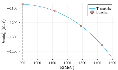
(a) Model I: repulsive potential: $c_{S}>0$

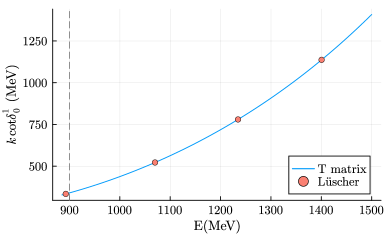
(b) Model I: attractive potential: $c_{S}<0$

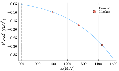
(c) Model II: repulsive potential: $c_{D}>0$

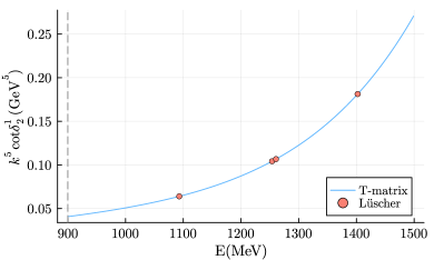
(d) Model II: attractive potential: $c_{D}<0$

Figure 1: Model I and II: $k_{\text{on}}\cot\delta^{1}_{0}$ and $k^{5}_{\text{on}}\cot\delta^{1}_{2}$ determined by standard Lüscher formula(solid circle) and partial wave LSE(solid line). The dashed line denotes the threshold $m_{1}+m_{2}$. The employed parameters are $|c_{S}|=4\times 10^{-5}/\text{MeV}^{2}$ and $|c_{D}|=3\times 10^{-3}/\text{MeV}^{2}$.

5.2 Model III

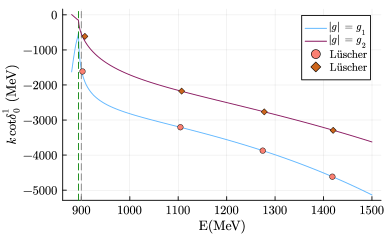
(a) repulsive potential: $c_{S}>0,\,g<0$

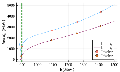
(b) attractive potential: $c_{S}<0,\,g>0$

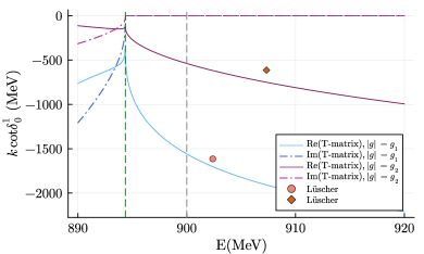
(c) detail near the threshold for (a)

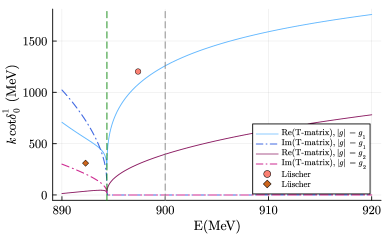
(d) detail near the threshold for (b)

Figure 2: Model III: $k_{\text{on}}\cot\delta^{1}_{0}$ determined by standard Lüscher formula(solid circle and diamond) and partial wave LSE(solid line). The gray and green dashed lines denote the threshold and endpoint of left-hand cut, respectively. Subfigures (c) and (d) provide detailed views of regions (a) and (b) near the threshold, offering a clearer perspective of the deviations is these regions. Below the left-hand cut, $k_{\text{on}}\cot\delta^{1}_{0}$ determined by partial wave LSE acquires a non-zero imaginary component, depicted by the dot-dashed line. The employed parameters are $(c_{S},g_{1},g_{2})=(1,1,5)\times 10^{-5}/\text{MeV}^{2}$

We now introduce the $S$-wave component of the long-range interaction into Model I to investigate the effect arising from the left-hand cut. We continue to take $\{E_{n}\}$ as input to obtain $[T^{J=1}_{00}]_{\text{L\"{u}scher}}$ via Eq. (74) and compare it to $[T^{J=1}_{00}]_{\text{Ham}}$ derived from Hamiltonian formalism. The results for various values of $c_{S}$ and $g$ are presented in the Fig. 2. We now make some discussions on the observations.

Firstly, at the the energy levels above the lowest one, $[T^{J=1}_{00}]_{\text{L\"{u}scher}}$ remains in agreement with the exact $[T^{J=1}_{00}]_{\text{Ham}}$, regardless of whether the interaction is attractive or repulsive. This suggests that the energy levels far from the left-hand cut are scarcely affected, and the standard Lüscher formula remains valid in this regime.

Secondly, for the lowest energy level, $[T^{J=1}_{00}]_{\text{L\"{u}scher}}$ apparently diverges from the exact $[T^{J=1}_{00}]_{\text{Ham}}$, regardless of whether it is below or above the threshold or left-hand cut. The deviation is related to the coupling strength $g$. The reason is that the lowest energy level is close to the left-hand cut so they experience the inescapable effect from the cut. The greater the role of the long-range interaction play, the more pronounced the deviation from the standard Lüscher formula.

Thirdly, for the attractive interactions, the lowest finite volume energy level can lie below the left-hand cut if the coupling is sufficiently strong. Under such conditions, the exact $k_{\text{on}}\cot\delta^{1}_{0}$ acquires a non-zero imaginary part. To be more specific, note that $k_{\text{on}}\cot\delta^{1}_{0}=ik_{\text{on}}+k_{\text{on}}(\rho T^{J=1}_{00})^{-1}$, where $T(E)=V+VG(E+i\epsilon)T(E)$. The unitarity of $S$-matrix ensures that $ik_{\text{on}}$ is always canceled by the corresponding factor in $T$-matrix arising from the propagator $G(E+i\epsilon)$. Consequently, $k_{\text{on}}\cot\delta^{1}_{0}$ remains real above the threshold if the potential is real (or hermitian). However, below the left-hand cut, due to the negative argument in log function, $V^{J=1}_{00}(k_{\text{on}},k_{\text{on}})$ introduces an additional non-vanishing imaginary part, which can not be canceled and ultimately results in the complex $k_{\text{on}}\cot\delta^{1}_{0}$. In contrast, the $k_{\text{on}}\cot\delta^{1}_{0}$ derived from standard Lüscher formula is always real when $q^{2}=\left(\frac{k_{\text{on}}L}{2\pi}\right)^{2}\in\mathbb{R}$. Therefore, at the energy below the left-hand cut, the standard Lüscher formula suffers a much more severe problem, as it violates the analyticity of the scattering matrix.

At this point, we would like to make a comment on the application of the Unitarized Chiral Perturbation Theory(UChPT) in the finite volume proposed in Ref. Doring:2011vk . Within the framework of UChPT in the infinite volume, it is concluded that, under a certain renormalization procedure, only the on-shell point of the potential contributes to the LSE. Consequently, the integral equation degenerates into a algebraic equation. When turning to the finite volume, it is concluded that the finite volume energy levels for a single partial wave and single channel system are determined by the equation:

$$V^{-1}(E)-\tilde{G}(E)=0,$$ (77)

where $\tilde{G}(E)\sim\frac{1}{L^{3}}\sum\limits_{\vec{n}}\frac{\omega_{1}+\omega_{2}}{\omega_{1}\omega_{2}}\frac{1}{E^{2}-(\omega_{1}+\omega_{2})^{2}}$. However, we argue that the Eq. (77) cannot be applicable in the presence of long-range interaction, at least below the left-hand cut, since $\tilde{G}(E)$ is real but $V^{-1}(E)$ becomes complex so Eq. (77) will never yield a real energy solution in that regime.

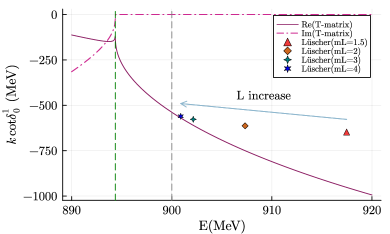
(a) repulsive potential: $c_{S}>0\,,g<0$

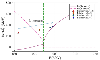
(b) attractive potential: $c_{S}<0\,,g>0$

Figure 3: Model III: Same as Figs. 2(c,d) with $|g|=g_{2}$. The solid makers denote the $k_{\text{on}}\cot\delta^{1}_{0}$ determined by standard Lüscher formula at several $L$, specifically $m_{\text{eff}}L=1.5,\,2,\,3,\,4$.

At last, in Fig. 3 we also present the $[T^{J=1}_{00}]_{\text{L\"{u}scher}}$ for the first energy level at several other values of $L$, specifically for $m_{\text{eff}}L=1.5,3,4$. It is evident that $[T^{J=1}_{00}]_{\text{L\"{u}scher}}$ converges to the exact $[T^{J=1}_{00}]_{\text{Ham}}$ as $L$ increases. The effect of the left-hand cut can be significant when $m_{\text{eff}}L$ is sufficiently small. In the presence of non-negligible long-range interaction, the Lüscher formula remains applicable only when $L$ is sufficiently large such that $m_{\text{eff}}L\gtrsim 4$ and the lowest energy level is above the left-hand cut. Unfortunately, this is impractical for the realistic systems whose $m_{\text{eff}}$ are quite small.

To gain further insight into these issues, we now briefly review the derivation of the standard ($S$-wave only) Lüscher formula. We focus initially on the above-threshold regime and subsequently perform the analytical continuation. The finite volume energy corresponds to the pole of $T^{L}(E)$ whose on-shell matrix elements are defined as Li:2024zld

$$T^{L}(k_{\text{on}},k_{\text{on}};E)=V(k_{\text{on}},k_{\text{on}})+\sum\limits_{\vec{q}}V(k_{\text{on}},q)G^{L}(q;E+i\epsilon)T^{L}(q,k_{\text{on}};E)\,,$$ (78)

where $q=|\vec{q}|$ and $G^{L}(q;E)=\left(\frac{2\pi}{L}\right)^{3}G(q;E)$. The Neumann series $T^{L}=\sum\limits_{n=0}^{\infty}V(G^{L}V)^{n}$ serves as a formal solution of Eq. (78). A key step in the derivation involves applying of Poisson formula:

$$\sum\limits_{\vec{q}}f(q)G^{L}(q;E+i\epsilon)=\sum\limits_{\vec{q}}\left(f(q)-f(k_{\text{on}})\right)G^{L}(q;E+i\epsilon)+f(k_{\text{on}})\sum\limits_{\vec{q}}G^{L}(q;E+i\epsilon)$$

$$=\int d\vec{q}\,f(q)G(q;E+i\epsilon)+f(k_{\text{on}})\left[\left(\frac{2\pi}{L}\right)^{3}\sum\limits_{\vec{q}}-\int d\vec{q}\right]G(q;E+i\epsilon)+\mathcal{O}(e^{-\kappa L})\,\,,$$ (79)

where $f(q)$ is assumed to be analytical in a strip including the real $q$-axis. The first term relates to the infinite volume contribution and the summation-minus-integration term encodes the finite volume effect which will ultimately lead to the Lüscher Zeta function. The exponential term, which is typically dropped, is given by the integral as

$$\mathcal{O}(e^{-\kappa L})\sim\sum\limits_{\vec{m}\neq\vec{0},\vec{m}\in\mathbb{Z}^{3}}\,\int d\vec{q}\,\frac{f(q)-f(k_{\text{on}})}{E-\omega_{1}(q)-\omega_{2}(q)+i\epsilon}\,e^{i\vec{m}\cdot\vec{q}L}$$ (80)

where $\kappa$ is a certain energy scale. For the realistic hadronic system with only short-range interaction, $\kappa\gtrsim m_{\pi}$. In order to illustrate the issue arising from long-range interaction, We now switch off the short-range interaction and apply the Poisson formula to the second term of Neumann series, i.e., the second term on the right-hand side of Eq. (78) with $T^{L}(q,k_{\text{on}};E)$ replaced by $V(q,k_{\text{on}})$. Then, $f(q;E)=\left[V^{S}_{\text{long-range}}(q,k_{\text{on}})\right]^{2}$ (Note that $f(q;E)$ also depends on $E$ implicitly), see Eq. (73). Due to the logarithm function, $f(q;E)$ features four branch cuts at $\pm k_{\text{on}}\pm iz$ with $z\geq m_{\text{eff}}$ on the complex $q$-plane. With the help of Cauchy theorem the integral in Eq. (80) can be converted into the integration along these branch cuts, which is expected to yield contributions of order $\mathcal{O}\left(A(E)e^{-m_{\text{eff}}L}\right)$, where $A(E)$ is a potentially $E$-dependent coefficient. As a consequence, the contribution from such exponential term may be underestimated if $m_{\text{eff}}$ is small enough, which disproves the neglect of it. Moreover, based on the previous observation, the coefficient $A(E)$ is expected to vanish as $E$ moves away from the left-hand cut, justifying the neglection of such term in that regime. In a word, in the above-threshold regime, the whole story is about the potential underestimated exponential term that is typically dropped in the derivation of Lüscher formula.

We now turn to the below-threshold regime. As shown in the subsection  5.1, the standard Lüscher formula can be safely analytically continued to the below-threshold regime in the absence of long-range interactions. However, this continuation is invalid in the presence of left-hand cut. Note that since $f(q;E)$ relates to the half on-shell elements of $V^{S}_{\text{long-range}}$, the most left-hand side of Eq. (5.2) is a analytical function of $E$ below the threshold along the real axis. In contrast, dropping the exponential term, the summation-minus-integration term in the right-hand side of the equation involves $f(k_{\text{on}}(E);E)$, which introduces a left-hand cut on the real $E$-axis. Therefore, Eq. (5.2) cannot be valid below the left-hand cut. (The continuation into the regime above the left-hand cut but below the threshold remains safe.) Obviously, it is the separation of on-shell point that ruins the continuation in the presence of long-range interaction Hansen:2024ffk , which is a necessary step when applying the Poisson formula above the threshold to get Lüscher formula.

5.3 Model IV

We now turn to the complete model, in which energy levels also receive contributions from higher partial waves. As in the previous subsections, we firstly calculate the energy levels $\{E_{n}\}$ and the scattering matrix elements $[T^{J}_{ll}]_{\text{Ham}}$ using the Hamiltonian method. Due to the inclusion of high partial wave, additional energy levels emerge compared to Model III. These new levels are initially degenerate with the non-interacting energies. As an distinct advantage of the Hamiltonian method, we are able to quantitatively analyze the contributions of different partial waves to $E_{n}$. Specifically, this can be achieved using the identity $\bra{E_{n}}\hat{V}_{L}\ket{E_{n}}=E_{n}-\bra{E_{n}}H_{0}\ket{E_{n}}$ where $\ket{E_{n}}$ denotes the eigenvector corresponding to $E_{n}$. On the other hand, $\hat{V}_{L}$ can also be expressed as the partial-wave expansion as follows,

$$\hat{V}_{L}=\left(\frac{2\pi}{L}\right)^{3}\sum\limits_{N^{\prime},N}\sum\limits_{l,J}V^{J}_{ll}\left(\sum\limits_{M=-J}^{J}\ket{N^{\prime},l,J,M}\bra{N,l,J,M}\right),$$ (81)

where

$$\ket{N,l,J,M}=\begin{cases}\delta_{l0}\delta_{J1}\sqrt{\frac{1}{4\pi}}\ket{\vec{0},M}\quad&\text{if}\,N=0\\ \sum\limits_{m,\lambda}C^{JM}_{lm,1\lambda}\sum\limits_{\vec{n}\,,\vec{n}^{2}=N}Y_{lm}(\vec{n})\ket{\vec{n},\lambda}\quad&\text{if}\,N\neq 0\end{cases},$$ (82)

which is similar to that in Eq. (10). Therefore, the contribution from $(l,J)$-component to $\bra{E_{n}}\hat{V}_{L}\ket{E_{n}}$, denoted by $[f^{J}_{ll}]_{n}$, is given by

$$[f^{J}_{ll}]_{n}=\left(\frac{2\pi}{L}\right)^{3}\sum\limits_{N^{\prime},N}V^{J}_{l,l}\left(\frac{2\pi\sqrt{N^{\prime}}}{L},\frac{2\pi\sqrt{N}}{L}\right)\sum\limits_{M=-J}^{J}\langle E_{n}|N^{\prime},l,J,M\rangle\langle N,l,J,M|E_{n}\rangle.$$ (83)

The $f^{J}_{ll}$ at few lowest levels are then examined. As examples, we present the $f^{J}_{ll}$ for an attractive interaction in Tabs. 2 and  3.

On the other hand, because of the inclusion of high partial waves, the complete standard Lüscher formula is now given by

$$\det\left[\delta_{ll^{\prime\prime}}\delta_{JJ^{\prime\prime}}\delta_{rr^{\prime\prime}}+i\rho\sum\limits_{l^{\prime},J^{\prime},r^{\prime}}\delta_{JJ^{\prime}}\delta_{rr^{\prime}}T^{J}_{l^{\prime},l}\left(\delta_{l^{\prime}l^{\prime\prime}}\delta_{J^{\prime}J^{\prime\prime}}\delta_{r^{\prime}r^{\prime\prime}}+i\mathcal{M}_{l^{\prime}J^{\prime}r^{\prime},l^{\prime\prime}J^{\prime\prime}r^{\prime\prime}}\right)\right]=0,$$ (84)

where $r$ is occurrence of $\Gamma$-irrep in $D^{J}$. For the first three energy levels that are 1) far from left-hand cut and 2) mainly contributed by $f^{J=1}_{00}$, we derive the $[T^{J=1}_{00}]_{\text{L\"{u}shcer,S-wave}}$ using Eq. (74) and $[T^{J=1}_{00}]_{\text{L\"{u}shcer,higher waves}}$ using Eq. (84). The latter incorporates a truncation of $l\leq 4,J\leq 4$ and takes $[T^{J=1,3}_{22}]_{\text{Ham}},[T^{J=3,4}_{44}]_{\text{Ham}}$ as input. The relevant $\mathcal{M}$-function are provided in Appendix C. By comparing two results, we are able to estimate the contributions of some high partial wave components from another perspective. The results are presented in Fig. 4.

$n$	1	$2^{*}$	3	$4^{*}$	5	6	$7^{*}$	8
$\Delta E_{\text{free}}$	0.0	199.1		366.7			514.3
$\Delta E_{n}$	-3.6	186.0	198.5	350.3	366.0	366.1	506.6	513.7
$\bra{E_{n}}\hat{V}_{L}\ket{E_{n}}$	-4.2	-15.3	-0.6	-17.2	-0.6	-0.6	-7.6	-0.6
$f^{1}_{00}$	-4.1	-14.5	0.0	-16.2	0.0	0.0	-6.9	0.0
$f^{1}_{22}$	0.0	0.0	-0.1	0.0	-0.1	-0.04	0.0	-0.08
$f^{3}_{22}$	0.0	0.0	-0.2	0.0	-0.1	-0.06	0.0	-0.06
$f^{3}_{44}$	-0.5 E-5	-0.06	-0.02	-0.01	-0.01	-0.04	-0.02	-0.01
$f^{4}_{44}$	-0.7 E-5	-0.07	-0.04	-0.01	-0.01	-0.1	-0.03	-0.02
$f^{5}_{44}$	-0.8 E-5	-0.09	-0.03	-0.01	-0.06	-0.1	-0.04	-0.08
$\sum f$	-4.1	-14.7	-0.39	-16.2	-0.28	-0.34	-7.0	-0.25

Table 2: Model IV: Contributions to energy levels from different partial wave components for the attractive potential characterized by $(c_{S},g)=(-2,0.5)\times 10^{-5}/\text{MeV}^{2}$. $\Delta E_{\text{free}}(\Delta E_{n})$ denotes the difference between $E_{\text{free}}(E_{n})$ and threshold $m_{1}+m_{2}$. The quantity $\sum f$ is the sum $\sum_{l\leq 4,J\leq 5}f^{J}_{ll}$. During the evaluation of $f^{J}_{ll}$, we truncate the momentum with $N\leq 10$ in Eq. (83), since the higher momentum components of $\ket{E_{n}}$ are supposed to negligible at low $E_{n}$. Energy levels marked with an asterisk ($*$) correspond to the solid circles in Fig. 4. All dimensional quantities in the table are presented in the units of MeV.

$n$	1	$2^{*}$	3	$4^{*}$	5	6	$7^{*}$	8
$\Delta E_{\text{free}}$	0.0	199.1		366.7			514.3
$\Delta E_{n}$	-8.1	180.2	194.5	344.3	361.9	362.0	501.7	509.5
$\bra{E_{n}}\hat{V}_{L}\ket{E_{n}}$	-8.9	-21.9	-4.6	-23.3	-4.8	-4.7	-12.5	-4.9
$f^{1}_{00}$	-8.8	-18.1	0.0	-19.3	0.0	0.0	-8.2	0.0
$f^{1}_{22}$	0.0	0.0	-0.9	0.0	-0.94	-0.31	0.0	-0.67
$f^{3}_{22}$	0.0	0.0	-1.3	0.0	-0.63	-0.47	0.0	-0.44
$f^{3}_{44}$	-0.5E-3	-0.5	-0.1	-0.1	-0.04	-0.34	-0.2	-0.06
$f^{4}_{44}$	-0.7E-3	-0.6	-0.3	-0.1	-0.10	-0.86	-0.2	-0.14
$f^{5}_{44}$	-0.9E-3	-0.7	-0.2	-0.1	-0.44	-0.64	-0.3	-0.62
$\sum f$	-8.8	-19.9	-2.8	-19.6	-2.2	-2.6	-8.9	-1.9

Table 3: Model IV: Same as Tab. 2, but with stronger coupling parameters $(c_{S},g)=(-2,4)\times 10^{-5}/\text{MeV}^{2}$.

Several discussions can be made based on the results. Firstly, from Tabs. 2 and 3, it is found that either $f_{00}^{J=1}=0,f^{J=1,3}_{22}\neq 0$ or vice versa, indicating that $E_{n}$ would not be simultaneously affected by $V^{J=1}_{00}$ and $V^{J=1,3}_{22}$. This result is straightforward to understand when Eq. (84) is truncated with $l\leq 2$ since in our toy model there is $T^{J}_{l^{\prime}l}\propto\delta_{l^{\prime}l}$ (which does not hold in general cases) and $\mathcal{M}_{2J,01}=\mathcal{M}_{01,2J}=0$ so Eq. (84) is factorized into two decoupled equations, namely, Eq. (74) and Eq. (75). We expect such factorization to hold even when no truncation is made.

Secondly, as shown in Fig. 4, it is evident that the $[T^{J=1}_{00}]_{\text{L\"{u}shcer,S-wave}}$ exhibits larger deviations from the $[T^{J=1}_{00}]_{\text{Ham}}$ as $g$ and $E_{n}$ increases. This observation aligns with the results in Tabs. 2 and  3, where $f^{J}_{ll\geq 2}$ becomes increasingly significant for larger $g$ and $E_{n}$. For a deeper insight, we switch off the short-range part and present the partial wave expansion of the potential $V_{00}(k\hat{e_{z}},k\hat{e_{z}})$ with truncation $J\leq J_{max}$ in Fig. 5. Near the lowest lattice momentum mode $k=0$, contributions from the high partial waves are highly suppressed and partial wave expansion converges rapidly, as expected. However, even near the second lowest mode, $k=\frac{2\pi}{L}\approx 300$ MeV, the contributions from higher partial waves become significant and the expansion converges much more slowly, as also mentioned in Refs. Epelbaum:2004fk ; Meng:2021uhz . The convergence may be even worse in the finite volume when $S$-wave contribution are not sufficiently dominant. As an example, for the fifth and sixth energy levels in Tab. 3, $\sum_{l\leq 4,J\leq 5}f^{J}_{ll}$ accounts for only half of the total contributions.

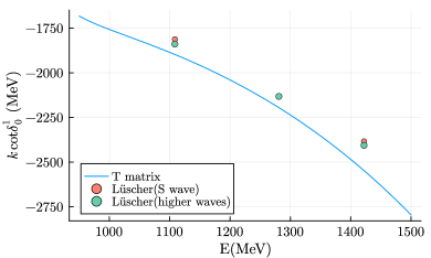
(a) repulsive potential: $c_{S}>0,\,g<0$

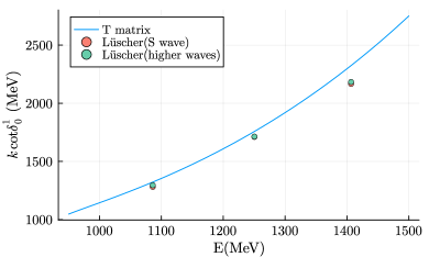
(b) attractive potential: $c_{S}<0,\,g>0$

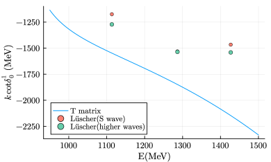
(c) repulsive potential: $c_{S}>0,\,g<0$

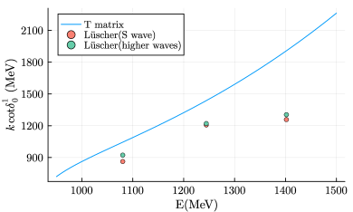
(d) attractive potential: $c_{S}<0,\,g>0$

Figure 4: Model IV: $k_{\text{on}}\cot\delta^{1}_{0}$ determined by standard Lüscher formula(solid circles) and partial wave LSE(solid line). The orange and green solid circles, which corresponds to the energy levels mainly contributed by the $S$-wave components of potential, are determined by Eq.(74) and Eq.(84), respectively. The employed parameters are $|c_{S}|=2\times 10^{-5}/\text{MeV}^{2}$ and $|g|=0.5\times 10^{-5}/\text{MeV}^{2}$ for the top row or $|g|=4\times 10^{-5}/\text{MeV}^{2}$ for the bottom row.

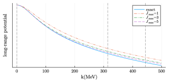
Figure 5: Model IV: partial wave expansion of potential $|V_{00}(k\hat{e}_{z},k\hat{e_{z}})|$ with truncation $J\leq J_{max}$ and $c_{S}=0$. The $y$-axis is set as log scale. The vertical gray dashed lines from left to right denote the lowest three lattice momentum $k=0,\frac{2\pi}{L}$ and $\frac{2\sqrt{2}\pi}{L}$.

Thirdly, in Fig. 4, $[T^{J=1}_{00}]_{\text{L\"{u}shcer, higher waves}}$ undergoes a noticeable shift compared to $[T^{J=1}_{00}]_{\text{L\"{u}shcer, S wave}}$ at the first and the third energy, while it remains nearly unchanged at the second energy. This can also be explained from Tabs. 2 and  3. It is found that $f^{J=3,4}_{44}$ at the second energy are quite small, rendering the corrections from $(l,J)=(4,3),(4,4)$ to Lüshcer formula are negligible. To achieve a noticeable shift at this energy the even higher partial waves $l\geq 6$ needs to be included in the truncation. In conclusion, higher partial waves can have sizable contribution to lattice energy levels and Lüscher formula, particularly when long-range interaction is sufficiently strong.

5.4 Conclusion

While some calculations in this section are specific to the current toy model, most of the conclusions are universal. In summary, the Hamiltonian method is equivalent to the Lüshcer formula up to a negligible exponential suppressed correction when long-range interaction is absent. However, when the long-range interaction becomes significant and left-hand cut approaches the threshold, the standard Lüscher formula gets in trouble in the energy region near the cut and requires modification. This issue becomes particularly severe if a lattice energy locates lies below the left-hand cut, as the standard Lüshcer formula violates the analyticity of the scattering matrix in this case. Moreover, if the long-range interaction is potentially significant, careful consideration of the contributions from high partial waves is suggested, when applying the standard Lüscher formula to describe high lattice energy levels. Neglecting these contributions can lead to inaccuracies in this case.

In practice, HEFT provides a convenient and efficient framework to bridge the finite volume energy levels and infinite volume scattering observables when the long-range potential is significant. The long-range part of the potential, which is generally constrained by experimental data, can be fixed (with potential assumptions such as the pion-mass dependence of coupling constant) during fitting the lattice energy levels. The short-range part of the potential can be parameterized with a few parameters, whose model-independence is guaranteed by (modified) Lüscher formula. Bubna:2024izx ; Raposo:2023oru

6 A more realistic application: $\chi_{c1}(3872)$

As a more realistic application, we calculate the finite volume energy levels of $I=0$ sector of $D\bar{D}^{*}+c.c.$ in the $T_{1}^{+}$ irrep, where the signal of the well-known exotic state $\chi_{c1}(3872)$, also known as $X(3872)$, can be observed. The discovery of $\chi_{c1}(3872)$ at 2003 starts a new era for hadron physics Belle:2003nnu . Since its observation, numerous phenomenological studies have been conducted to explore the nature of $\chi_{c1}(3872)$. Possible interpretations include a compact tetraquark or, more convincingly, a molecular bound state of $D\bar{D}^{*}$, mixed with $c\bar{c}$ core known as $\chi_{c1}(2P)$. We refer to Refs. Guo:2017jvc ; Brambilla:2019esw ; Chen:2016qju ; Esposito:2016noz for a comprehensive summary of the relevant phenomenological studies.

The signal of $\chi_{c1}(3872)$ has also been observed in lattice studies. Refs. Li:2024pfg ; Prelovsek:2013cra ; Lee:2014uta report the identification of a candidate for $\chi_{c1}(3872)$ using lattice QCD with $D\bar{D}^{*}$ and $c\bar{c}$ interpolators. Furthermore, the coupling of $\chi_{c1}(3872)$ to the $c\bar{c}$ core is suggested to be strong in Ref. Padmanath:2015era ; Bali:2011rd . More recently, the $D\bar{D}^{*}(I=0)$ scattering at four different $m_{\pi}$ has been studied. A bound state corresponding to $\chi_{c1}(3872)$ was reported at the highest $m_{\pi}$ by applying standard Lüscher formula Li:2024pfg .

In this section, we calculate the energy levels based on the model built in Ref. Wang:2023ovj , which successfully reproduces the binding energy of $\chi_{c1}(3872)$ as well as the line shape of $T_{cc}$ and $Z_{c}(3900)$ Yu:2024sqv . As mentioned earlier, the $\chi_{c1}(3872)$ can be interpreted as a mixture of $c\bar{c}$ core and a $D\bar{D}^{*}$ molecular component. The interaction between $\ket{D\bar{D}^{*}}$ states is given by the following potential:

$$V^{D\bar{D}^{*}}(\vec{p},\vec{k})=\frac{1}{2(2\pi)^{3}}\left(-3\bar{V}^{u}_{\pi}-3\bar{V}^{u}_{\rho}-\bar{V}^{u}_{\omega}+3\bar{V}^{t}_{\rho}+\bar{V}^{t}_{\omega}\right)\left(\frac{\Lambda^{2}}{\Lambda^{2}+\vec{k}^{2}}\right)^{2}\left(\frac{\Lambda^{2}}{\Lambda^{2}+\vec{p}^{2}}\right)^{2},$$ (85)

where the coefficients are the isospin factor. Note that the isospin breaking effect is not accounted for in this model. This is consistent with the current lattice simulation, which assumes $m_{u}=m_{d}$. Specifically, $\bar{V}^{t,u}_{\pi,\rho,\omega}=\frac{1}{2}\left(V^{t,u}_{\pi,\rho,\omega}(q_{t,u})+V^{t,u}_{\pi,\rho,\omega}(\tilde{q}_{t,u})\right)$ and

$$V^{u}_{\pi}(q) =-\left(\frac{g}{f_{\pi}}\right)^{2}\frac{\left(q\cdot\epsilon\right)\left(q\cdot\epsilon^{*}\right)}{q^{2}-m_{\pi}^{2}}$$ (86)

$$V^{u}_{\rho,\omega}(q) =-2\left(g_{v}\lambda\right)^{2}\frac{\left(q\cdot\epsilon\right)\left(q\cdot\epsilon^{*}\right)-q^{2}\left(\epsilon^{*}\cdot\epsilon\right)}{q^{2}-m_{\rho,\omega}^{2}}$$ (87)

$$V^{t}_{\rho,\omega}(q) =\frac{1}{2}\left(g_{v}\beta\right)^{2}\frac{\epsilon\cdot\epsilon^{*}}{q^{2}-m_{\rho,\omega}^{2}}$$ (88)

where

$$q_{u} =\left(\omega_{D^{*}}(\vec{k})-\omega_{D}(\vec{p}),\,\vec{p}+\vec{k}\right)\quad,\quad\tilde{q}_{u}=\left(\omega_{D^{*}}(\vec{p})-\omega_{D}(\vec{k}),\,\vec{p}+\vec{k}\right)$$ (89)

$$q_{t} =\left(\omega_{D^{*}}(\vec{k})-\omega_{D^{*}}(\vec{p}),\,\vec{p}+\vec{k}\right)\quad,\quad\tilde{q}_{t}=\left(\omega_{D}(\vec{p})-\omega_{D}(\vec{k}),\,\vec{p}+\vec{k}\right)$$ (90)

where $\epsilon$ denotes the polarization or helicity vector given in Appendix B. The parameters used are: $g=0.57$, $f_{\pi}=132.0$ MeV, $g_{v}=5.8$, $\beta=0.687$, $\lambda=0.683$/GeV and $\Lambda=1.0$ GeV. All particle masses, except for $m_{\pi}$, are taken as physical values. We set $m_{\pi}=150$ MeV, which is slightly higher than the physical value to avoid the three-body decay $D^{*}\to D\pi$. Otherwise, the system, strictly speaking, should be treated as a three-particle system. Based on the Quark-Pair-Creation(QPC) model, the pure $S$-wave interaction between the $\ket{c\bar{c}}$ and $\ket{D\bar{D}^{*}}$ is given by

$$V^{c\bar{c}}(\vec{k}_{D\bar{D}^{*}})=\gamma I_{D\bar{D}^{*},c\bar{c}}(|\vec{k}_{D\bar{D}^{*}}|)$$ (91)

where $\gamma=4.69$ represents the amplitude of producing the light quark pair and $I_{D\bar{D}^{*},c\bar{c}}$ is the overlap of the meson wave functions. The mass of $c\bar{c}$ core is set as $m_{\chi_{c1}(2P)}=3.95$ GeV. Further details of the QPC model can be found in Ref. Micu:1968mk .

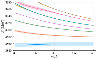
(a) full model

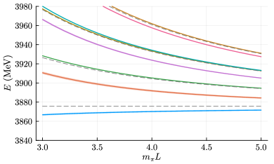
(b) model excluding $V^{c\bar{c}}$

Figure 6: Finite volume energy levels of $\chi_{c1}(3872)$ in $T_{1}^{+}$-irrep. The dashed lines denote the non-interacting energy of $D\bar{D}^{*}$. The shaded bands denote the uncertainty.

The energy levels in $T_{1}^{+}$-irrep calculated using full model and the model excluding $V^{c\bar{c}}$ are presented in the Fig. 6. The shaded bands denote the uncertainties estimated by bootstrapping parameter errors in the model. The uncertainty of $\gamma$ is not explicitly provided in the literature, but it is expected to be large. Here, we adopt $\gamma=4.69$ and manually assign a relative error of $10\%$ for analysis. In both cases, the energy levels are qualitatively consistent with the lattice results reported in Refs. Li:2024pfg ; Prelovsek:2013cra ; Lee:2014uta . Specifically speaking, there is a level below the $D\bar{D}^{*}$ threshold, a level situated between the non-interacting energies $D\bar{D}^{*}(\absolutevalue{\vec{n}}^{2}=1)$ and $D\bar{D}^{*}(\absolutevalue{\vec{n}}^{2}=2)$, and a level very close to and slightly above the non-interacting energy of $D\bar{D}^{*}(\absolutevalue{\vec{n}}^{2}=2)$. As in the previous section, the contributions from the different partial waves to the energy levels $f^{J}_{l^{\prime},l}$ are analyzed, with the results summarized in the Tab. 4. The first and the second energy levels are primarily contributed by the $S$-wave component. The third energy level is predominantly influenced by $V^{J=1,3}_{22}$, reflecting $D$-wave dominance. Note that although the third energy can be extracted by a $S$-wave interpolator due to the partial wave mixing as in Ref. Li:2024pfg , the $S$-wave Lüshcer formula cannot be applied to get the $S$-wave phase shift for this level. Furthermore, a energy situated between the non-interacting energies $D\bar{D}^{*}(\absolutevalue{\vec{n}}^{2}=2)$ and $D\bar{D}^{*}(\absolutevalue{\vec{n}}^{2}=3)$ is anticipated if more interpolators are employed.

$m_{\pi}L$	3			4			5
$n$	1	2	3	1	2	3	1	2	3
$\bra{E_{n}}\hat{V}_{L}\ket{E_{n}}$	-50.80	-23.03	0.74	-55.24	-12.98	0.57	-58.06	-6.46	0.33
$f^{1}_{00}$($V^{c\bar{c}}$)	-23.88	-12.83	-0.20	-25.87	-6.88	-0.10	-26.76	-3.32	-0.04
$f^{1}_{00}(V^{D\bar{D}^{*}})$	-12.57	-2.44	-0.01	-13.43	-1.92	-0.02	-13.38	-1.00	-0.01
$f^{1}_{02}=f^{1}_{20}$	-3.07	-0.74	0.13	-1.97	-0.30	0.08	-1.16	-0.08	0.03
$f^{1}_{22}$	0.01	0.00	0.73	0.02	0.00	0.40	0.01	0.00	0.23
$f^{3}_{22}$	0.02	0.00	0.47	0.00	0.00	0.32	0.00	0.00	0.19

Table 4: Contributions from several lowest partial wave components to the finite volume energy levels of the full model for $\chi_{c1}(3872)$ at $m_{\pi}L=3,4,5$. $f^{1}_{00}(V^{c\bar{c}})$ and $f^{1}_{00}(V^{D\bar{D}^{*}})$ denote the diagonal $S$-wave contribution from $V^{c\bar{c}}$ and $V^{D\bar{D}^{*}}$, respectively.

By comparing the qualitative behavior of energy levels as a function of $L$ in the subfigures of Fig. 6, we can discern the difference arising from the $c\bar{c}$ core. As depicted by the pink line, the presence of the $c\bar{c}$ core causes an energy level near the $m_{\chi_{c1}(2P)}$ to align closely with a lower non-interacting energy level at small $L$ and transition toward a higher non-interacting level as $L$ increases. Furthermore, it is possible for some energy levels to intersect with the non-interacting as shown in Fig. 7. The intersection corresponds to a Castillejo-Dalitz-Dyson(CDD) zeros arising from the competition between $V^{c\bar{c}}$ and $V^{D\bar{D}^{*}}$ interactions Castillejo:1955ed ; Li:2022aru ; Yang:2022vdb . The observation of these two behaviors will imply the existence of $c\bar{c}$ core. However, we acknowledge the significant technical challenges involved on lattice QCD, as these observations require lattice data of very high precision across multiple values of $L$.

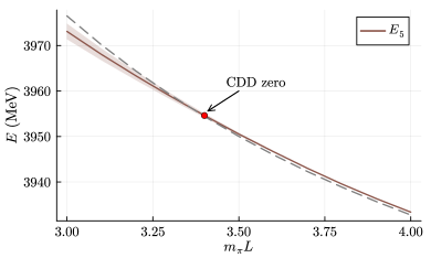
(a) full model

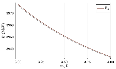
(b) model excluding $V^{c\bar{c}}$

Figure 7: Detail of the fifth energy level in Fig.6. The red circle in the left subfigure indicates the intersection with the non-interacting energy, suggesting the presence of a CDD zero due to the competition between $V^{c\bar{c}}$ and $V^{D\bar{D}^{*}}$. No intersection is found in the right subfigure.

7 Summary

In this paper, we introduce a systematic and sophisticated method for performing the irrep decomposition of the finite volume Hamiltonian for the two-particle system with general potential and arbitrary spins. This framework is applicable to systems in both the rest or moving frames. Based on the method, we provide the explicit expressions for matrix elements of finite volume effective Hamiltonian, offering a practical and user-friendly approach for readers who wish to apply Hamiltonian method to address the left-hand cut issue on the lattice. The method inherently incorporates the isospin symmetry and can be straightforwardly generalized into the three-particle system in the foreseeable future.

Utilizing this method, we investigate several toy models to compare the Hamiltonian method with the standard Lüscher formula. The two frameworks agree pretty well when long-range interaction is absent. However, in the presence of long range interaction, the standard Lüscher formula needs modification near the left-hand cut, especially for the energies situated below the left-hand cut. The influence of left-hand cut decreases as the size of finite volume increases. Furthermore, higher energy levels can receive the non-negligible contributions from the higher partial waves if the long-range interactions play a significant role. Therefore, to obtain the reliable results, the careful examination of the partial wave truncation is suggested when applying the standard Lüscher formula to these energy levels.

In addition, we calculate the finite volume spectrum of $\chi_{c1}(3872)$ using HEFT with the phenomenological model given in Refs. Wang:2023ovj ; Yu:2024sqv where the binding energy and line shapes of $T_{cc}$ and $Z_{c}(3900)$ are successfully reproduced. Our spectrum is qualitatively consistent with the lattice spectrum provided in Refs. Li:2024pfg ; Prelovsek:2013cra ; Lee:2014uta . We also explore the contributions from different partial waves to energy levels and examined the impact of $c\bar{c}$ core. This approach effectively addresses challenging problems in lattice QCD and holds potential for applications to the study of other exotic states in hadron physics.

Appendix A Conventions of symmetry group

In this appendix we clarify our conventions of the symmetry groups and their irreducible representations. Though the finite volume effective Hamiltonian are equivalent up to a similarity transformation and its eigenvalues are exactly identical, the specific expression of $I$-matrix and its eigenvectors differ from the conventions adopted. We follow the conventions in the Refs. Bernard:2008ax ; Doring:2018xxx ; Morningstar:2013bda and provide a brief summary here.

For $O_{h}$, we follow the conventions in Refs. Bernard:2008ax ; Doring:2018xxx . The 48 elements of $O_{h}$ can be divide into two subsets: $g_{i}$ with $i=1,\cdots\,,24$ making up $O$ group, and another 24 elements generated by multiplying parity inversion, $g_{i}=\mathbb{P}g_{i-24}$ for $25\leq i\leq 48$. As outlined in Tab. 2 of the Ref. Bernard:2008ax , $g_{i}$ with $1\leq i\leq 24$ are uniquely parameterized by a angle $\omega$ with $-\pi\leq\omega<\pi$ and a unit vector $\vec{m}$ with $m_{z}\geq 0$. The $O_{h}$ group has ten bosonic irrep $A_{1}^{\pm},A_{2}^{\pm},E^{\pm},T_{1}^{\pm},T_{2}^{\pm}$ with respecitve dimensions $1,1,2,3,3$. The specific matrix expressions for these irreps are provided in Tab. 1 of Ref. Doring:2018xxx , where the matrix elements are all real.

The order of ${}^{2}O_{h}$ is as twice as that of $O_{h}$. For each element $g\in O_{h}$ specified by $(\vec{m},\omega)$ there is a counterpart element $\bar{g}\in{}^{2}O_{h}$ specified by $(\vec{m},\omega+2\pi)$. The irreps of $O_{h}$ are also the irreps of ${}^{2}O_{h}$. Besides, there are six additional fermionic irreps, $G_{1}^{\pm},G_{2}^{\pm},H^{\pm}$. For bosonic irrep, $D^{\Gamma}(\bar{g})=D^{\Gamma}(g)$, while for fermonic irrep, $D^{\Gamma}(\bar{g})=-D^{\Gamma}(g)$. The specific matrix expressions are provided in Ref. Bernard:2008ax . Briefly speaking, the matrices of $G_{1}$ and $H$ corresponds to the Wigner-D matices $D^{J=\frac{1}{2}}$ and $D^{J=\frac{3}{2}}$, respectively. The relationship between $G_{1}$ and $G_{2}$ is the same as that between $A_{1}$ and $A_{2}$ as well as $T_{1}$ and $T_{2}$.

For the moving system, the lattice symmetry groups are the subgroup of $O_{h}$: $C_{4v}$, $C_{2v}$ and $C_{3v}$ or their double cover for $\frac{\vec{P}L}{2\pi}=(0,0,1),\,(0,1,1)\,,(1,1,1)$, respectively. As the subgroup of $O_{h}$, the group elements are given by $C_{4v}=\{g_{1},g_{14},g_{15},g_{24},g_{42},g_{43},g_{46},g_{47}\}$, $C_{3v}=\{g_{1},g_{2},g_{3},g_{41},g_{43},g_{45}\}$ and $C_{2v}=\{g_{1},g_{16},g_{41},g_{46}\}$. For other directions like $\frac{\vec{P}L}{2\pi}=(1,0,0)$ and $(1,1,0)$ we refer to Ref. Wu:2021xvz . We follow the Ref. Morningstar:2013bda for the conventions of the irreps of these groups. Roughly speaking, for $C_{4v}$ there are five irreps $A_{1},A_{2},B_{1},B_{2},E$ and two additional ones $G_{1},G_{2}$ for its double cover. The dimensions of these irreps are $1,1,1,1,2$ and $2,2$, respectively. For $C_{2v}$, there are four irreps $A_{1},A_{2},B_{1},B_{2}$ and one additional one $G$ for its double cover. The dimensions are $1,1,1,1$ and $2$, respectively. (Note that the definitions of $B_{1}$ and $B_{2}$ here are reversed compared to Ref. Dudek:2012gj ; Dudek:2012xn .) For $C_{3v}$, there are three irreps $A_{1},A_{2},E$ and three additional ones $F_{1},F_{2},G$ for its double cover. The dimensions are $1,1,2$ and $1,1,2$, respectively. The correspondence of the notations of generators in Ref. Morningstar:2013bda and here are as follows: $(C_{4z},I_{s}C_{2y})\leftrightarrow(g_{15},g_{47})$ for $C_{4v}$, $(C_{3\delta},I_{s}C_{2b})\leftrightarrow(g_{3},g_{43})$ for $C_{3v}$ and $(C_{2e},I_{s}C_{2f})\leftrightarrow(g_{16},g_{41})$ for $C_{2v}$, respectively. The specific matrix expressions of the generators for different irreps are provided in the Tab.(12-14) of Ref. Morningstar:2013bda . The matices for other elements can be obtained by appropriate multiplication. For convenience we present the multiplication as follows:

• For $C_{4v}$: $g_{1}=g_{15}^{4},\,g_{14}=g_{15}^{3},\,g_{24}=g_{15}^{2},\,g_{42}=g_{47}g_{15},\,g_{43}=g_{47}g_{15}^{3},\,g_{46}=g_{47}g_{15}^{2}$

• For $C_{3v}$: $g_{1}=g_{3}^{3},\,g_{2}=g_{3}^{2},\,g_{41}=g_{43}g_{3},\,g_{45}=g_{43}g_{3}^{2}$

• For $C_{2v}$: $g_{1}=g_{16}^{2},\,g_{46}=g_{41}g_{16}$

• For ${}^{2}C_{4v}$: $g_{1}=g_{15}^{8},\,g_{14}=g_{15}^{7},\,g_{24}=g_{15}^{6},\,g_{42}=g_{47}g_{15},\,g_{43}=g_{47}g_{15}^{3},\,g_{46}=g_{47}g_{15}^{2}$

• For ${}^{2}C_{3v}$: $g_{1}=g_{3}^{6},\,g_{2}=g_{3}^{5},\,g_{41}=g_{43}g_{3},\,g_{45}=g_{43}g_{3}^{2}$

• For ${}^{2}C_{2v}$: $g_{1}=g_{16}^{4},\,g_{46}=g_{41}g_{16}$

Appendix B Polarization vector and helicity vector

In this appendix we present the polarization vector $\epsilon(\vec{p},\lambda)$ and helicty vector $\epsilon_{H}(\vec{p},\underline{\lambda})$ for a spin-$1$ particle with $\vec{p}=\left(p,\theta,\phi\right)$ and mass $m$. For polarization vectorweinberg2005quantum ,

$$\epsilon(\vec{p},\lambda=0) =\begin{pmatrix}\frac{p}{m}\cos\theta\\ \left(\frac{E}{m}-1\right)\cos\theta\sin\theta\cos\phi\\ \left(\frac{E}{m}-1\right)\cos\theta\sin\theta\sin\phi\\ 1+\left(\frac{E}{m}-1\right)\cos^{2}\theta\end{pmatrix}$$ (92)

$$\epsilon(\vec{p},\lambda=-1) =\sqrt{\frac{1}{2}}\begin{pmatrix}\frac{p}{m}\sin\theta\,e^{i\phi}\\ 1+\left(\frac{E}{m}-1\right)\sin\theta\cos\phi\,e^{i\phi}\\ -i+\left(\frac{E}{m}-1\right)\sin\theta\sin\phi\,e^{i\phi}\\ \left(\frac{E}{m}-1\right)\cos\theta\,e^{i\phi}\end{pmatrix}$$ (93)

$$\epsilon(\vec{p},\lambda=+1) =-\epsilon^{*}(\vec{p},\lambda=-1)$$ (94)

For helicity vector, by definition, $\epsilon_{H}(\vec{p},\underline{\lambda})=\sum\limits_{\lambda}e^{-i\lambda\phi}d^{s}_{\lambda\underline{\lambda}}(\theta)\epsilon(\vec{p},\lambda)$

$$\epsilon_{H}(\vec{p},\underline{\lambda}=0) =\begin{pmatrix}\frac{p}{m}\\ \frac{E}{m}\frac{\vec{p}}{\absolutevalue{\vec{p}}}\end{pmatrix}$$ (95)

$$\epsilon_{H}(\vec{p},\underline{\lambda}=+1) =\sqrt{\frac{1}{2}}\begin{pmatrix}0\\ -\cos\theta\cos\phi+i\sin\phi\\ -\cos\theta\sin\phi-i\cos\phi\\ \sin\theta\end{pmatrix}$$ (96)

$$\epsilon_{H}(\vec{p},\underline{\lambda}=-1) =-\epsilon_{H}^{*}(\vec{p},\underline{\lambda}=+1)$$ (97)

Appendix C Specific expressions of the pertinent Lüshcer function

In this appendix we present the specific expressions of the symmetric Lüscher functions $\mathcal{M}_{l^{\prime}J^{\prime},lJ}=\mathcal{M}_{lJ,l^{\prime}J^{\prime}}$ that are pertinent to this work. For the general definition of $\mathcal{M}$ we refer to Ref. Woss:2018irj .

$$\mathcal{M}_{01,01} =\mathcal{M}_{21,21}=\frac{2\mathcal{Z}_{00}(1;q^{2})}{\sqrt{\pi}k_{\text{on}}L}$$ (98)

$$\mathcal{M}_{21,23} =-\frac{2}{7\pi}\sqrt{\frac{6}{\pi}}\mathcal{Z}_{40}(1;q^{2})$$ (99)

$$\mathcal{M}_{23,23} =\frac{2}{\pi}\left[\frac{1}{q}\sqrt{\frac{1}{4\pi}}\mathcal{Z}_{00}(1;q^{2})+\frac{1}{q^{5}}\frac{1}{7\sqrt{\pi}}\mathcal{Z}_{40}(1;q^{2})\right]$$ (100)

$$\mathcal{M}_{01,43} =-\frac{2}{3\pi^{3/2}}\frac{1}{q^{5}}\mathcal{Z}_{40}(1;q^{2})$$ (101)

$$\mathcal{M}_{21,43} =\frac{20}{21\left(2\pi\right)^{3/2}}\frac{1}{q^{5}}\mathcal{Z}_{40}(1;q^{2})$$ (102)

$$\mathcal{M}_{23,43} =-\frac{2}{\pi}\left[\frac{1}{q^{5}}\frac{5}{77}\sqrt{\frac{3}{\pi}}\mathcal{Z}_{40}(1;q^{2})+\frac{1}{q^{7}}\frac{25}{11\sqrt{39\pi}}\mathcal{Z}_{60}(1;q^{2})\right]$$ (103)

$$\mathcal{M}_{43,43} =\frac{2}{\pi}\left[\frac{1}{q}\sqrt{\frac{1}{4\pi}}\mathcal{Z}_{00}(1;q^{2})+\frac{1}{q^{5}}\frac{27}{154\sqrt{\pi}}\mathcal{Z}_{40}(1;q^{2})+\frac{1}{q^{7}}\frac{25}{66\sqrt{13\pi}}\mathcal{Z}_{60}(1;q^{2})\right]$$ (104)

$$\mathcal{M}_{01,44} =\frac{2\sqrt{2}}{\pi}\frac{1}{q^{5}}\sqrt{\frac{1}{5\pi}}\mathcal{Z}_{44}(1;q^{2})$$ (105)

$$\mathcal{M}_{21,44} =\frac{2\sqrt{2}}{\pi}\frac{1}{q^{5}}\sqrt{\frac{1}{10\pi}}\mathcal{Z}_{44}(1;q^{2})$$ (106)

$$\mathcal{M}_{23,44} =\frac{2\sqrt{2}}{\pi}\left[-\frac{1}{q^{5}}\frac{3}{11}\sqrt{\frac{3}{5\pi}}\mathcal{Z}_{44}(1;q^{2})+\frac{1}{q^{7}}\frac{5}{11}\sqrt{\frac{3}{13\pi}}\mathcal{Z}_{64}(1;q^{2})\right]$$ (107)

$$\mathcal{M}_{43,44} =\frac{2\sqrt{2}}{\pi}\left[-\frac{1}{q^{5}}\frac{9}{22\sqrt{5\pi}}\mathcal{Z}_{44}(1;q^{2})+\frac{1}{q^{7}}\frac{15}{22\sqrt{13\pi}}\mathcal{Z}_{64}(1;q^{2})\right]$$ (108)

$$\mathcal{M}_{44,44} =\frac{2}{\pi}\left[\frac{1}{q}\sqrt{\frac{1}{4\pi}}\mathcal{Z}_{00}(1;q^{2})-\frac{1}{q^{3}}\frac{17}{22\sqrt{5\pi}}\mathcal{Z}_{20}(1;q^{2})+\frac{1}{q^{5}}\frac{27}{286\sqrt{\pi}}\mathcal{Z}_{40}(1;q^{2})+\right.$$ (109)

$$\quad+\left.\frac{1}{q^{7}}\frac{1}{110\sqrt{13\pi}}\mathcal{Z}_{60}(1;q^{2})+\frac{1}{q^{9}}\frac{896}{715\sqrt{17\pi}}\mathcal{Z}_{80}(1;q^{2})\right]$$ (110)

where $q=\frac{k_{\text{on}}L}{2\pi}$ and Lüscher Zeta function

$$\mathcal{Z}_{lm}(s;x^{2})=\sum\limits_{\vec{n}\in\mathbb{Z}^{3}}\frac{\absolutevalue{\vec{n}}^{l}Y_{lm}(\vec{n})}{\left(\vec{n}^{2}-x^{2}\right)^{s}}.$$

The method for numerical evaluation of Lüscher Zeta function can be found in Ref. Gockeler:2012yj .

Appendix D Ingredients for matrix elements

In subsection 4.6 the expression of matrix element is provided. There are two parts, namely, kinematical part and dynamical part. The kinematical part is independent of the effective potential and entirely determined by the symmetry group and reference momentum. For convenience, we explicitly present the ingredients for kinematical part here.

It should be noted that many results depend on the conventions of irreps and the choices of reference momentum, though the eigenvalues of Hamiltonian are invariant under different conventions and choices. Our conventions of irreps and reference momentum have been discussed in Appendix A and Sec. 4, respectively. For convenience we provide the reference momentum $\vec{n}_{o}$ for $O_{h}$ with $|\vec{n}_{o}|\leq 100$ as: $(0,0,0)$, $(0,0,1)$, $(0,1,1)$, $(1,1,1)$, $(0,0,2)$, $(0,1,2)$, $(1,1,2)$, $(0,2,2)$, $(0,0,3)$, $(2,2,1)$, $(0,1,3)$, $(1,1,3)$, $(2,2,2)$, $(0,2,3)$, $(1,2,3)$, $(0,0,4)$, $(0,1,4)$, $(2,2,3)$, $(1,1,4)$, $(0,3,3)$, $(3,3,1)$, $(0,2,4)$, $(1,2,4)$, $(3,3,2)$, $(2,2,4)$, $(0,0,5)$, $(0,3,4)$, $(0,1,5)$, $(1,3,4)$, $(1,1,5)$, $(3,3,3)$, $(0,2,5)$, $(2,3,4)$, $(1,2,5)$, $(0,4,4)$, $(2,2,5)$, $(4,4,1)$, $(0,3,5)$, $(3,3,4)$, $(1,3,5)$, $(0,0,6)$, $(4,4,2)$, $(0,1,6)$, $(1,1,6)$, $(2,3,5)$, $(0,2,6)$, $(1,2,6)$, $(0,4,5)$, $(4,4,3)$, $(1,4,5)$, $(3,3,5)$, $(2,2,6)$, $(0,3,6)$, $(2,4,5)$, $(1,3,6)$, $(4,4,4)$, $(0,0,7)$, $(2,3,6)$, $(0,1,7)$, $(0,5,5)$, $(3,4,5)$, $(1,1,7)$, $(5,5,1)$, $(0,4,6)$, $(0,2,7)$, $(1,4,6)$, $(1,2,7)$, $(3,3,6)$, $(5,5,2)$, $(2,4,6)$, $(2,2,7)$, $(4,4,5)$, $(0,3,7)$, $(1,3,7)$, $(5,5,3)$, $(0,5,6)$, $(3,4,6)$, $(2,3,7)$, $(1,5,6)$, $(0,0,8)$, $(0,1,8)$, $(0,4,7)$, $(2,5,6)$, $(1,1,8)$, $(1,4,7)$, $(5,5,4)$, $(3,3,7)$, $(0,2,8)$, $(4,4,6)$, $(1,2,8)$, $(2,4,7)$, $(3,5,6)$, $(2,2,8)$, $(0,6,6)$, $(0,3,8)$, $(6,6,1)$, $(1,3,8)$, $(0,5,7)$, $(3,4,7)$, $(1,5,7)$, $(5,5,5)$, $(6,6,2)$, $(2,3,8)$, $(4,5,6)$, $(2,5,7)$, $(0,4,8)$, $(0,0,9)$, $(1,4,8)$, $(4,4,7)$, $(6,6,3)$, $(0,1,9)$, $(3,3,8)$, $(1,1,9)$, $(3,5,7)$, $(2,4,8)$, $(0,2,9)$, $(0,6,7)$, $(1,2,9)$, $(1,6,7)$, $(5,5,6)$, $(6,6,4)$, $(2,2,9)$, $(0,5,8)$, $(3,4,8)$, $(2,6,7)$, $(0,3,9)$, $(1,5,8)$, $(4,5,7)$, $(1,3,9)$, $(2,5,8)$, $(2,3,9)$, $(3,6,7)$, $(4,4,8)$, $(0,4,9)$, $(6,6,5)$, $(1,4,9)$, $(3,5,8)$, $(0,7,7)$, $(3,3,9)$, $(7,7,1)$, $(5,5,7)$, $(0,0,10)$, $(0,6,8)$.

The elements of little group $\text{LG}(\vec{n}_{o})$ and the corresponding left coset are presented in Tab. 5. For double cover group, the order of little group doubles while the left cosets remain unchanged. Specifically, if $g$ is an element of $\text{LG}(\vec{n}_{o})\subset G$, then both $g$ and $\bar{g}$ are elements of $\text{LG}(\vec{n}_{o})\subset{}^{2}G$.

The normalized eigenvectors with nonzero eigenvalues of $I$-matrix for $K\pi$, $N\pi$ and $\rho\pi$ system are presented in Tabs. 6-8. To make use of them correctly, several issues deserves to be mentioned:

1. Results for the patterns $(a,b,c),\,(a,b,*)_{1},\,(*,a,b)_{2},\,(a,b,c)_{3}$ are not shown since the their little group contains only the identity element and therefore $I^{\Gamma}=\mathbb{I}$. (Note that the helicity index needs to take all the values $\underline{\lambda}=-s,\cdots,s$ for these patterns.)

2. For $N\pi$ and $\rho\pi$ it is sufficient to present the results for non-negative helicity because, as shown in Tab. 5, $\text{LG}^{-}(\vec{n}_{o})$ are nonempty for all the patterns of $\vec{n}_{o}$ in Tabs. 7 and  8.

3. For $N\pi$ and $\rho\pi$ with $\vec{P}\neq 0$, the $I$-matrix may not entirely determined by the pattern of $\vec{n}_{o}$. For example, both $\vec{n}_{o}=(0,0,1)$ and $(0,0,-1)$ belong to $(0,0,*)_{1}$ but their $I$-matrix are not exactly the same. The reason is their little group contains non-trivial proper elements and the corresponding Wigner angle are different. Fortunately, the $I$-matrix for the system with $\vec{P}=0$ are entirely determined by the pattern of $\vec{n}_{o}$ since either the pattern entirely determines the direction of $\vec{n}_{o}$ or the only proper element in $\text{LG}(\vec{n}_{o})$ is identity element.

The Wigner rotation angle $\varphi_{w}(\vec{n}_{o},g)$ for $g\in\text{LC}(\vec{n}_{o})$ is also required. With the help of Mathematica or other scientific languages, they can be computed straightforwardly from their definition. For brevity, explicit results are not shown here. It is worth emphasizing that, for bosonic systems, $\varphi_{w}$ can be calculated using either bosonic or fermionic Wigner-D matrices. However, for fermionic systems, the fermionic Wigner-D matrices must be used or $\varphi_{w}$ may differ by $2\pi$, which makes difference.

	pattern	$\text{LG}(\vec{n}_{o})=\left\{g_{i}\right\}$	$\text{LC}(\vec{n}_{o})=\left\{g_{i}\right\}$
$O_{h}$	$(0,0,0)$	$i=1,\cdots,48$	$i=1$
	$(0,0,a)$	$i=1,14,15,24,42,43,46,47$	$i=1,2,3,4,6,18$
	$(0,a,a)$	$i=1,16,41,46$	$i=1,\cdots,10,11,17$
	$(a,a,a)$	$i=1,2,3,41,43,45$	$i=1,4,5,6,10,11,12,17$
	$(0,a,b)$	$i=1,46$	$i=1\cdots,24$
	$(a,a,b)$ or $(b,b,a)$	$i=1,43$	$i=1,\cdots,24$
	$(a,b,c)$	$i=1$	$i=1,\cdots,48$
$C_{4v}$	$(0,0,*)_{1}$	$i={1},{14},{15},{24},{42},{43},{46},{47}$	$i=1$
	$(0,a,*)_{1}$	$i=1,46$	$i=1,14,15,24$
	$(a,a,*)_{1}$	$i=1,43$	$i=1,14,15,24$
	$(a,b,*)_{1}$	$i=1$	$i={1},{14},{15},{24},{42},{43},{46},{47}$
$C_{2v}$	$(0,a,a)_{1}$	$i=1,16,41,46$	$i=1$
	$(0,a,b)_{2}$	$i=1,46$	$i=1,16$
	$(*,a,a)_{2}$	$i=1,41$	$i=1,16$
	$(*,a,b)_{2}$	$i=1$	$i=1,16,41,46$
$C_{3v}$	$(a,a,a)_{3}$	$i=1,2,3,41,43,45$	$i=1$
	$(a,a,b)_{3}$	$i=1,43$	$i=1,2,3$
	$(a,b,c)_{3}$	$i=1$	$i=1,2,3,41,43,45$

Table 5: The little group $\text{LG}(\vec{n}_{o})$ and the chosen left coset element $\text{LC}(\vec{n}_{o})$ for $O_{h}$, $C_{4v}$, $C_{2v}$ and $C_{3v}$. The conventions of elements are discussed in Appendix A.

$G$	pattern	$\text{[eigenvectors]}^{\Gamma}$
$O_{h}$	$(0,0,0)$	$\left[(1)\right]^{A_{1}^{+}}$
	$(0,0,a)$	$\left[(1)\right]^{A_{1}^{+}}$, $\left[(1,0)\right]^{E^{+}}$, $\left[(0,0,1)\right]^{T_{1}^{-}}$
	$(0,a,a)$	$\left[(1)\right]^{A_{1}^{+}}$, $\left[\frac{1}{2}\left(-1,\sqrt{3}\right)\right]^{E^{+}}$, $\left[\frac{1}{\sqrt{2}}\left(0,1,1\right)\right]^{T_{1}^{-}}$, $\left[(1,0,0)\right]^{T_{2}^{+}}$, $\left[\frac{1}{\sqrt{2}}\left(0,-1,1\right)\right]^{T_{2}^{-}}$
	$(a,a,a)$	$\left[(1)\right]^{A_{1}^{+},\,A_{2}^{-}}$, $\left[\frac{1}{\sqrt{3}}\left(1,1,1\right)\right]^{T_{1}^{-},\,T_{2}^{+}}$
	$(0,a,b)$	$\left[(1)\right]^{A_{1}^{+},\,A_{2}^{+}}$, $\left[(0,1),\,(1,0)\right]^{E^{+}}$, $\left[(1,0,0)\right]^{T_{1}^{+},\,T_{2}^{+}}$, $\left[\left(0,0,1\right),\left(0,1,0\right)\right]^{T_{1}^{-},\,T_{2}^{-}}$
	$(a,a,b)$	$\left[(1)\right]^{A_{1}^{+},\,A_{2}^{-}}$, $\left[(1,0)\right]^{E^{+}}$, $\left[(0,1)\right]^{E^{-}}$, $\left[\frac{1}{\sqrt{2}}\left(-1,1,0\right)\right]^{T_{1}^{+},\,T_{2}^{-}}$
	or $(b,b,a)$	$\left[\left(0,0,1\right),\frac{1}{\sqrt{2}}\left(1,1,0\right)\right]^{T_{1}^{-},\,T_{2}^{+}}$
$C_{4v}$	$(0,0,*)_{1}$	$\left[(1)\right]^{A_{1}}$
	$(0,a,*)_{1}$	$\left[(1)\right]^{A_{1},B_{1}},\left[(0,1)\right]^{E}$
	$(a,a,*)_{1}$	$\left[(1)\right]^{A_{1},\,B_{2}},\left[\frac{1}{\sqrt{2}}\left(1,1\right)\right]^{E}$
$C_{2v}$	$(0,a,a)_{2}$	$\left[(1)\right]^{A_{1}}$
	$(0,a,b)_{2}$	$\left[(1)\right]^{A_{1},\,B_{2}}$
	$(*,a,a)_{2}$	$\left[(1)\right]^{A_{1},\,B_{1}}$
$C_{3v}$	$(a,a,a)_{3}$	$[(1)]^{A_{1}}$
	$(a,a,b)_{3}$	$[(1)]^{A_{1}},\,[(0,1)]^{E}$

Table 6: The normalized eigenvectors with nonzero eigenvalue of $I$-matrix for $K\pi$-system. The intrinsic parity is assumed to be positive.

$G$	pattern	$\text{[eigenvectors]}^{\Gamma}_{\underline{\lambda}=+\frac{1}{2}}$
${}^{2}O_{h}$	$(0,0,a)$	$\left[(1,0)\right]^{G_{1}^{\pm}}$, $\left[(0,1,0,0)\right]^{H^{\pm}}$
	$(0,a,a)$	$\left[\frac{\left((\sqrt{2}+1)i,\,1\right)}{\sqrt{4+2\sqrt{2}}}\right]^{G_{1}^{\pm}}$, $\left[\frac{\left((-\sqrt{2}+1)i,\,1\right)}{\sqrt{4-2\sqrt{2}}}\right]^{G_{2}^{\pm}}$,
		$\left[\frac{\left(i(2-\sqrt{2}),\,\sqrt{3}-\sqrt{6},\,0,\,1\right)}{\sqrt{16-10\sqrt{2}}},\,\frac{\left(-\sqrt{3}+\sqrt{6},\,i(2-\sqrt{2}),\,1,\,0\right)}{\sqrt{16-10\sqrt{2}}}\right]^{H^{\pm}}$
	$(a,a,a)$	$\left[\frac{\left((1+i)(1+\sqrt{3}),\,2\right)}{2\sqrt{3+\sqrt{3}}}\right]^{G_{1}^{\pm},G_{2}^{\pm}}$, $\left[\frac{\left((1-i)(1+\sqrt{3}),\,2i,\,(1+i)(1+\sqrt{3}),\,2\right)}{2\sqrt{2(3+\sqrt{3})}}\right]^{H^{\pm}}$
	$(0,a,b)$	$\left[\left(0,1\right),\left(1,0\right)\right]^{G_{1}^{\pm},G_{2}^{\pm}}$, $\left[\left(1,0,0,0\right),\left(0,1,0,0\right),\left(0,0,1,0\right),\left(0,0,0,1\right)\right]^{H^{\pm}}$
	$(a,a,b)$	$\left[\left(0,1\right),\left(1,0\right)\right]^{G_{1}^{\pm},G_{2}^{\pm}}$, $\left[\left(1,0,0,0\right),\left(0,1,0,0\right),\left(0,0,1,0\right),\left(0,0,0,1\right)\right]^{H^{\pm}}$
	or $(b,b,a)$
${}^{2}C_{4v}$	$(0,0,*)_{1}$	$\left[(1,0)\right]^{G_{1}}(\text{if}\,\,*>0),\,\left[(0,1)\right]^{G_{1}}(\text{if}\,\,*<0)$
	$(0,a,*)_{1}$	$\left[\left(1,0\right),\left(0,1\right)\right]^{G_{1},G_{2}}$
	$(a,a,*)_{1}$	$\left[\left(1,0\right),\left(0,1\right)\right]^{G_{1},G_{2}}$
${}^{2}C_{2v}$	$(0,a,a)_{2}$	$\left[\frac{1}{\sqrt{2}}\left(i,1\right)\right]^{G}$
	$(0,a,b)_{2}$	$\left[\left(0,1\right),\left(1,0\right)\right]^{G}$
	$(*,a,a)_{2}$	$\left[\left(0,1\right),\left(1,0\right)\right]^{G}$
${}^{2}C_{3v}$	$(a,a,a)_{3}$	$\left[\frac{\left((1+i)(\sqrt{3}+1),2\right)}{2\sqrt{3+\sqrt{3}}}\right]^{G}$
	$(a,a,b)_{3}$	$\left[(1)\right]^{F_{1},\,F_{2}}$, $\left[(1,0),(0,1)\right]^{G}$

Table 7: The normalized eigenvectors with nonzero eigenvalue of $I$-matrix for $N\pi$-system. The intrinsic parity is assumed to be positive.

$G$	pattern	$\text{[ eigenvectors ]}^{\Gamma}_{\underline{\lambda}\geq 0}$
$O_{h}$	$(0,0,a)$	$\left[(1)\right]^{A_{1}^{-}}_{0}$ $\left[(1,0)\right]^{E^{-}}_{0},\left[(0,0,1)\right]^{T_{1}^{+}}_{0}$, $\left[\frac{1}{\sqrt{2}}\left(i,1,0\right)\right]^{T_{1}^{\pm}}_{1}$, $\left[\frac{1}{\sqrt{2}}(-i,1,0)\right]_{1}^{T_{2}^{\pm}}$
	$(0,a,a)$	$\left[(1)\right]^{A_{1}^{-}}_{0},\,\left[\frac{1}{2}(-1,\sqrt{3})\right]_{0}^{E^{-}},\,\left[\frac{1}{\sqrt{2}}(0,1,1)\right]_{0}^{T_{1}^{+}},\,\left[\frac{1}{\sqrt{2}}(0,-1,1)\right]_{0}^{T_{2}^{+}},\,\left[(1,0,0)\right]_{0}^{T_{2}^{-}}$,
		$\left[(1)\right]_{1}^{A_{2}^{\pm}},\,\left[\frac{1}{2}(\sqrt{3},1)\right]_{1}^{E^{\pm}},\,\left[(1,0,0),\frac{1}{\sqrt{2}}(0,-1,1)\right]_{1}^{T_{1}^{\pm}},\left[\frac{1}{\sqrt{2}}(0,1,1)\right]_{1}^{T_{2}^{\pm}}$
	$(a,a,a)$	$\left[(1)\right]_{0}^{A_{1}^{-},\,A_{2}^{+}},\,\left[\frac{1}{\sqrt{3}}(1,1,1)\right]_{0}^{T_{1}^{+},\,T_{2}^{-}},\,\left[\frac{1}{\sqrt{2}}(i,1)\right]_{1}^{E^{\pm}},\,\left[\frac{1}{\sqrt{3}}(e^{-\frac{2\pi i}{3}},e^{\frac{2\pi i}{3}},1)\right]_{1}^{T_{1}^{\pm},T_{2}^{\pm}}$
	$(0,a,b)$	$\left[(1)\right]_{0}^{A_{1}^{-},\,A_{2}^{-}}$, $\left[(0,1),(1,0)\right]_{0}^{E^{-}}$, $\left[(0,1,0),(0,0,1)\right]_{0}^{T_{1}^{+},T_{2}^{+}}$, $\left[(1,0,0)\right]_{0}^{T_{1}^{-},T_{2}^{-}}$,
		$\left[(1)\right]_{1}^{A_{1}^{\pm},\,A_{2}^{\pm}}$, $\left[(0,1),(1,0)\right]_{1}^{E^{\pm}}$, $\left[(1,0,0),(0,1,0),(0,0,1)\right]_{1}^{T_{1}^{\pm},T_{2}^{\pm}}$
	$(a,a,b)$	$\left[(1)\right]_{0}^{A_{1}^{-},\,A_{2}^{+}},\,\left[(0,1)\right]_{0}^{E^{+}},\,\left[(1,0)\right]_{0}^{E^{-}},\,\left[(-\frac{1}{\sqrt{2}},\frac{1}{\sqrt{2}},0)\right]_{0}^{T_{1}^{-},\,T_{2}^{+}}$
	or $(b,b,a)$	$\left[(0,0,1),(\frac{1}{\sqrt{2}},\frac{1}{\sqrt{2}},0)\right]_{0}^{T_{1}^{+},\,T_{2}^{-}}$,
		$\left[(1)\right]_{1}^{A_{1}^{\pm},\,A_{2}^{\pm}},\,\left[(0,1),(1,0)\right]_{1}^{E^{\pm}},\,\left[(1,0,0),(0,1,0),(0,0,1)\right]_{1}^{T_{1}^{\pm},\,T_{2}^{\pm}}$
$C_{4v}$	$(0,0,*)_{1}$	$\left[(1)\right]^{A_{2}}_{0},\,\left[\frac{1}{\sqrt{2}}(i,1)\right]^{E}_{1}(\text{if}\,\,*>0),\,\left[\frac{1}{\sqrt{2}}(-i,1)\right]^{E}_{1}(\text{if}\,\,*<0)$
	$(0,a,*)_{1}$	$[(1)]_{0}^{A_{2},\,B_{2}},\left[(1,0)\right]_{0}^{E}$, $\left[(1)\right]_{1}^{A_{1},\,A_{2},\,B_{1},\,B_{2}},\,\left[(1,0),(0,1)\right]_{1}^{E}$
	$(a,a,*)_{1}$	$\left[(1)\right]_{0}^{A_{2},B_{1}},\,\left[\frac{1}{\sqrt{2}}(-1,1)\right]_{0}^{E}$, $\left[(1)\right]_{1}^{A_{1},\,A_{2},\,B_{1},\,B_{2}},\,\left[(1,0),(0,1)\right]_{1}^{E}$
$C_{2v}$	$(0,a,a)_{2}$	$\left[(1)\right]_{0}^{A_{2}}$, $\left[(1)\right]_{1}^{B_{1},\,B_{2}}$
	$(0,a,b)_{2}$	$\left[(1)\right]_{0}^{A_{2},\,B_{1}}$, $\left[(1)\right]_{1}^{A_{1},\,A_{2},\,B_{1},\,B_{2}}$
	$(*,a,a)_{2}$	$\left[(1)\right]_{0}^{A_{2},\,B_{2}}$, $\left[(1)\right]_{1}^{A_{1},\,A_{2},\,B_{1},\,B_{2}}$
$C_{3v}$	$(a,a,a)_{3}$	$\left[(1)\right]_{0}^{A_{2}}$, $\left[\frac{1}{\sqrt{2}}(-i,1)\right]^{E}_{1}(\text{if}\,\,a>0),\,\left[\frac{1}{\sqrt{2}}(i,1)\right]^{E}_{1}(\text{if}\,\,a<0)$
	$(a,a,b)_{3}$	$\left[(1)\right]_{0}^{A_{2}},\left[(1,0)\right]_{0}^{E}$, $\left[(1)\right]_{1}^{A_{1},A_{2}}$, $\left[(1,0),(0,1)\right]_{1}^{E}$

Table 8: The normalized eigenvectors with nonzero eigenvalue of $I$-matrix for $\rho\pi$-system. The intrinsic parity is assumed to be positive.

References

- (1) M. Luscher, Two particle states on a torus and their relation to the scattering matrix, Nucl. Phys. B 354 (1991) 531.
- (2) K. Rummukainen and S.A. Gottlieb, Resonance scattering phase shifts on a nonrest frame lattice, Nucl. Phys. B 450 (1995) 397 [hep-lat/9503028].
- (3) M. Gockeler, R. Horsley, M. Lage, U.G. Meissner, P.E.L. Rakow, A. Rusetsky et al., Scattering phases for meson and baryon resonances on general moving-frame lattices, Phys. Rev. D 86 (2012) 094513 [1206.4141].
- (4) M.T. Hansen and S.R. Sharpe, Multiple-channel generalization of Lellouch-Luscher formula, Phys. Rev. D 86 (2012) 016007 [1204.0826].
- (5) C.h. Kim, C.T. Sachrajda and S.R. Sharpe, Finite-volume effects for two-hadron states in moving frames, Nucl. Phys. B 727 (2005) 218 [hep-lat/0507006].
- (6) C. Liu, X. Feng and S. He, Two particle states in a box and the S-matrix in multi-channel scattering, Int. J. Mod. Phys. A 21 (2006) 847 [hep-lat/0508022].
- (7) N. Li and C. Liu, Generalized Lüscher formula in multichannel baryon-meson scattering, Phys. Rev. D 87 (2013) 014502 [1209.2201].
- (8) R.A. Briceno, J.J. Dudek and R.D. Young, Scattering processes and resonances from lattice QCD, Rev. Mod. Phys. 90 (2018) 025001 [1706.06223].
- (9) H.A. Bethe, Theory of the Effective Range in Nuclear Scattering, Phys. Rev. 76 (1949) 38.
- (10) J.M. Blatt and J.D. Jackson, On the Interpretation of Neutron-Proton Scattering Data by the Schwinger Variational Method, Phys. Rev. 76 (1949) 18.
- (11) J.R. Taylor, Scattering theory: the quantum theory of nonrelativistic collisions, Courier Corporation (2012).
- (12) S. Weinberg, Lectures on Quantum Mechanics, Cambridge University Press (2013).
- (13) LHCb collaboration, Study of the doubly charmed tetraquark , Nature Commun. 13 (2022) 3351 [2109.01056].
- (14) LHCb collaboration, Observation of an exotic narrow doubly charmed tetraquark, Nature Phys. 18 (2022) 751 [2109.01038].
- (15) Y. Lyu, S. Aoki, T. Doi, T. Hatsuda, Y. Ikeda and J. Meng, Doubly Charmed Tetraquark Tcc+ from Lattice QCD near Physical Point, Phys. Rev. Lett. 131 (2023) 161901 [2302.04505].
- (16) M. Padmanath and S. Prelovsek, Signature of a Doubly Charm Tetraquark Pole in DD* Scattering on the Lattice, Phys. Rev. Lett. 129 (2022) 032002 [2202.10110].
- (17) M.T. Hansen, F. Romero-López and S.R. Sharpe, Incorporating DD effects and left-hand cuts in lattice QCD studies of the Tcc(3875)+, JHEP 06 (2024) 051 [2401.06609].
- (18) M.-L. Du, A. Filin, V. Baru, X.-K. Dong, E. Epelbaum, F.-K. Guo et al., Role of Left-Hand Cut Contributions on Pole Extractions from Lattice Data: Case Study for Tcc(3875)+, Phys. Rev. Lett. 131 (2023) 131903 [2303.09441].
- (19) A.B.a. Raposo and M.T. Hansen, Finite-volume scattering on the left-hand cut, JHEP 08 (2024) 075 [2311.18793].
- (20) L. Meng, V. Baru, E. Epelbaum, A.A. Filin and A.M. Gasparyan, Solving the left-hand cut problem in lattice QCD: Tcc(3875)+ from finite volume energy levels, Phys. Rev. D 109 (2024) L071506 [2312.01930].
- (21) S. Collins, A. Nefediev, M. Padmanath and S. Prelovsek, Toward the quark mass dependence of Tcc+ from lattice QCD, Phys. Rev. D 109 (2024) 094509 [2402.14715].
- (22) R. Bubna, H.-W. Hammer, F. Müller, J.-Y. Pang, A. Rusetsky and J.-J. Wu, Lüscher equation with long-range forces, JHEP 05 (2024) 168 [2402.12985].
- (23) H. van Haeringen and L.P. Kok, MODIFIED EFFECTIVE RANGE FUNCTION, Phys. Rev. A 26 (1982) 1218.
- (24) M.-L. Du, F.-K. Guo and B. Wu, Effective range expansion with the left-hand cut, 2408.09375.
- (25) HAL QCD collaboration, Hadron–hadron interactions from imaginary-time Nambu–Bethe–Salpeter wave function on the lattice, Phys. Lett. B 712 (2012) 437 [1203.3642].
- (26) J.M.M. Hall, A.C.P. Hsu, D.B. Leinweber, A.W. Thomas and R.D. Young, Finite-volume matrix Hamiltonian model for a system, Phys. Rev. D 87 (2013) 094510 [1303.4157].
- (27) J.-J. Wu, T.S.H. Lee, A.W. Thomas and R.D. Young, Finite-volume Hamiltonian method for coupled-channels interactions in lattice QCD, Phys. Rev. C 90 (2014) 055206 [1402.4868].
- (28) Y. Li, J.-j. Wu, D.B. Leinweber and A.W. Thomas, Hamiltonian effective field theory in elongated or moving finite volume, Phys. Rev. D 103 (2021) 094518 [2103.12260].
- (29) J.M.M. Hall, W. Kamleh, D.B. Leinweber, B.J. Menadue, B.J. Owen, A.W. Thomas et al., Lattice QCD Evidence that the (1405) Resonance is an Antikaon-Nucleon Molecule, Phys. Rev. Lett. 114 (2015) 132002 [1411.3402].
- (30) Z.-W. Liu, W. Kamleh, D.B. Leinweber, F.M. Stokes, A.W. Thomas and J.-J. Wu, Hamiltonian effective field theory study of the resonance in lattice QCD, Phys. Rev. Lett. 116 (2016) 082004 [1512.00140].
- (31) C.D. Abell, D.B. Leinweber, Z.-W. Liu, A.W. Thomas and J.-J. Wu, Low-lying odd-parity nucleon resonances as quark-model-like states, Phys. Rev. D 108 (2023) 094519 [2306.00337].
- (32) Z.-W. Liu, W. Kamleh, D.B. Leinweber, F.M. Stokes, A.W. Thomas and J.-J. Wu, Hamiltonian effective field theory study of the resonance in lattice QCD, Phys. Rev. D 95 (2017) 034034 [1607.04536].
- (33) J.-j. Wu, D.B. Leinweber, Z.-w. Liu and A.W. Thomas, Structure of the Roper Resonance from Lattice QCD Constraints, Phys. Rev. D 97 (2018) 094509 [1703.10715].
- (34) Z. Yang, G.-J. Wang, J.-J. Wu, M. Oka and S.-L. Zhu, Novel Coupled Channel Framework Connecting the Quark Model and Lattice QCD for the Near-threshold Ds States, Phys. Rev. Lett. 128 (2022) 112001 [2107.04860].
- (35) L. Meng and E. Epelbaum, Two-particle scattering from finite-volume quantization conditions using the plane wave basis, JHEP 10 (2021) 051 [2108.02709].
- (36) L. Meng, E. Ortiz-Pacheco, V. Baru, E. Epelbaum, M. Padmanath and S. Prelovsek, Doubly charm tetraquark channel with isospin from lattice QCD, 2411.06266.
- (37) Y. Li, J.-J. Wu, C.D. Abell, D.B. Leinweber and A.W. Thomas, Partial Wave Mixing in Hamiltonian Effective Field Theory, Phys. Rev. D 101 (2020) 114501 [1910.04973].
- (38) L. Meng and E. Epelbaum, Finite volume NN systems using plane wave expansion and eigenvector continuation, PoS LATTICE2022 (2023) 201.
- (39) M. Luscher, Volume Dependence of the Energy Spectrum in Massive Quantum Field Theories. 2. Scattering States, Commun. Math. Phys. 105 (1986) 153.
- (40) S.U. Chung, SPIN FORMALISMS, .
- (41) C.D. Abell, D.B. Leinweber, A.W. Thomas and J.-J. Wu, Regularization in nonperturbative extensions of effective field theory, Phys. Rev. D 106 (2022) 034506 [2110.14113].
- (42) V. Bernard, M. Lage, U.-G. Meissner and A. Rusetsky, Resonance properties from the finite-volume energy spectrum, JHEP 08 (2008) 024 [0806.4495].
- (43) M. Döring, H.W. Hammer, M. Mai, J.Y. Pang, t.A. Rusetsky and J. Wu, Three-body spectrum in a finite volume: the role of cubic symmetry, Phys. Rev. D 97 (2018) 114508 [1802.03362].
- (44) H.-J. Jing, S.-M. Wu and J.-J. Wu, Algorithms for partial wave amplitudes in the covariant L-S scheme, Phys. Rev. D 110 (2024) 016014 [2405.06576].
- (45) S. Weinberg, The Quantum Theory of Fields: Volume 1, Foundations, Cambridge University Press (2005).
- (46) Y. Li, J.-J. Wu, T.S.H. Lee and R.D. Young, Generalized boost transformations in finite volumes and application to Hamiltonian methods, JHEP 08 (2024) 178 [2404.16702].
- (47) J.J. Dudek, R.G. Edwards and C.E. Thomas, S and D-wave phase shifts in isospin-2 pi pi scattering from lattice QCD, Phys. Rev. D 86 (2012) 034031 [1203.6041].
- (48) Hadron Spectrum collaboration, Energy dependence of the resonance in elastic scattering from lattice QCD, Phys. Rev. D 87 (2013) 034505 [1212.0830].
- (49) A. Woss, C.E. Thomas, J.J. Dudek, R.G. Edwards and D.J. Wilson, Dynamically-coupled partial-waves in isospin-2 scattering from lattice QCD, JHEP 07 (2018) 043 [1802.05580].
- (50) M. Doring, U.-G. Meissner, E. Oset and A. Rusetsky, Unitarized Chiral Perturbation Theory in a finite volume: Scalar meson sector, Eur. Phys. J. A 47 (2011) 139 [1107.3988].
- (51) E. Epelbaum, W. Glockle and U.-G. Meissner, The Two-nucleon system at next-to-next-to-next-to-leading order, Nucl. Phys. A 747 (2005) 362 [nucl-th/0405048].
- (52) Belle collaboration, Observation of a narrow charmonium-like state in exclusive decays, Phys. Rev. Lett. 91 (2003) 262001 [hep-ex/0309032].
- (53) F.-K. Guo, C. Hanhart, U.-G. Meißner, Q. Wang, Q. Zhao and B.-S. Zou, Hadronic molecules, Rev. Mod. Phys. 90 (2018) 015004 [1705.00141].
- (54) N. Brambilla, S. Eidelman, C. Hanhart, A. Nefediev, C.-P. Shen, C.E. Thomas et al., The states: experimental and theoretical status and perspectives, Phys. Rept. 873 (2020) 1 [1907.07583].
- (55) H.-X. Chen, W. Chen, X. Liu and S.-L. Zhu, The hidden-charm pentaquark and tetraquark states, Phys. Rept. 639 (2016) 1 [1601.02092].
- (56) A. Esposito, A. Pilloni and A.D. Polosa, Multiquark Resonances, Phys. Rept. 668 (2017) 1 [1611.07920].
- (57) H. Li, C. Shi, Y. Chen, M. Gong, J. Liang, Z. Liu et al., Relevant Scattering in Lattice QCD, 2402.14541.
- (58) S. Prelovsek and L. Leskovec, Evidence for X(3872) from DD* scattering on the lattice, Phys. Rev. Lett. 111 (2013) 192001 [1307.5172].
- (59) Fermilab Lattice, MILC collaboration, Searching for the and on HISQ Lattices, 1411.1389.
- (60) M. Padmanath, C.B. Lang and S. Prelovsek, X(3872) and Y(4140) using diquark-antidiquark operators with lattice QCD, Phys. Rev. D 92 (2015) 034501 [1503.03257].
- (61) G.S. Bali, S. Collins and C. Ehmann, Charmonium spectroscopy and mixing with light quark and open charm states from =2 lattice QCD, Phys. Rev. D 84 (2011) 094506 [1110.2381].
- (62) G.-J. Wang, Z. Yang, J.-J. Wu, M. Oka and S.-L. Zhu, New insight into the exotic states strongly coupled with the from the , Sci. Bull. 69 (2024) 3036 [2306.12406].
- (63) K. Yu, G.-J. Wang, J.-J. Wu and Z. Yang, A Three-Coupled-Channel Analysis of Involving , , and , 2409.10865.
- (64) L. Micu, Decay rates of meson resonances in a quark model, Nucl. Phys. B 10 (1969) 521.
- (65) L. Castillejo, R.H. Dalitz and F.J. Dyson, Low’s scattering equation for the charged and neutral scalar theories, Phys. Rev. 101 (1956) 453.
- (66) Y. Li and J.-J. Wu, Inverse scattering problem with a bare state, Phys. Rev. D 105 (2022) 116024 [2204.05510].
- (67) Z. Yang, G.-J. Wang, J.-J. Wu, M. Oka and S.-L. Zhu, The investigations of the P-wave Bs states combining quark model and lattice QCD in the coupled channel framework, JHEP 01 (2023) 058 [2207.07320].
- (68) C. Morningstar, J. Bulava, B. Fahy, J. Foley, Y.C. Jhang, K.J. Juge et al., Extended hadron and two-hadron operators of definite momentum for spectrum calculations in lattice QCD, Phys. Rev. D 88 (2013) 014511 [1303.6816].
- (69) CSSM-QCDSF collaboration, Towards high partial waves in lattice QCD with an extended two-hadron operator, Phys. Rev. D 105 (2022) 074506 [2109.01557].