Cooperative Optimization of Grid-Edge Cyber and Physical Resources for Resilient Power System Operation

Abstract

The cooperative operation of grid-edge power and energy resources is crucial to improving the resilience of power systems during contingencies. However, given the complex cyber-physical nature of power grids, it is hard to respond timely with limited costs for deploying additional cyber and/or phyiscal resources, such as during a high-impact low-frequency cyber-physical event. Therefore, the paper examines the design of cooperative cyber-physical resource optimization solutions to control grid-tied cyber and physical resources. First, the operation of a cyber-physical power system is formulated into a constrained optimization problem, including the cyber and physical objectives and constraints. Then, a bi-level solution is provided to obtain optimal cyber and physical actions, including the reconfiguration of cyber topology (e.g., activation of communication links) in the cyber layer and the control of physical resources (e.g., energy storage systems) in the physical layer. The developed method improves grid resilience during cyberattacks and can provide guidance on the control of coupled physical side resources. Numerical simulation on a modified IEEE 14-bus system demonstrates the effectiveness of the proposed approach.

I Introduction

Power systems are inherently cyber-physical, with frequent and mandatory interactions between cyber and physical resources. In cyber-physical power systems (CPPSs), the operation of physical devices, such as generators, transformers, and loads, are integrated with the operation of cyber devices, such as routers, switches, and firewalls to continuously monitor, control, and optimize the grid performance [1]. Typically, the physical side of a CPPS is responsible for generating, transmitting, and distributing electric power. The physical side resources, such as distributed energy resources, have been proven valuable in providing ancillary services [2], enhancing grid efficiency, and improving grid resilience [3].

The majority of current work focuses on developing resilient physical power systems [4]. However, the physical operation of CPPSs heavily relies on cyber infrastructures that are prone to cyber threats, including all the digital and information technologies used to monitor, communicate, and control the physical assets [5, 6, 7]. To address the cyber threats, Sahu el al. [6] develop an automatic firewall configuration tool that can streamline the configuration of firewalls for utilities. To predict cyber risks, Rostami et al. [7] use a Bayesian attack graph to simulate attack paths and a Markov model to illustrate the consequences of attacks. Despite having distinct characteristics, ignoring the interconnectivity between cyber and physical layers could lead to failures in power system operation, especially under system contingencies. To enhance the resilience of CPPSs, another crucial perspective is to understand and learn the cooperation among grid cyber, physical, and cyber-physical components. For example, a tri-level optimization model is proposed in [8] to mitigate coordinated attacks on CPPSs, which involve physically short-circuiting transmission lines after compromising the communication network of protection relays. Besides, the development of redundant pathways and backup systems has proven efficacy in restoring operations during cyber-physical attacks [9].

Therefore, cooperative physical and cyber actions are essential to counteract malicious cyber-physical threats in CPPSs. In this paper, we investigate the cooperative optimization of grid-edge resources that interact between system operators and end-users for resilient power system operation. The contributions of this paper include: 1) Development of a synergized cyber-physical optimization framework that can be used to cooperatively operate cyber and physical resources in CPPSs; 2) Design a cyber topology reconfiguration and physical power system restoration strategy; and 3) Provide bi-level optimal cyber and physical response actions to enhance grid resilience during synthetic cyber-physical events.

In the rest of this paper, Section II presents the formulation of a CPPS. Section III designs the resilient cyber and physical system operation strategy. Section IV provides numerical simulation results. Section V concludes the paper.

II Problem Formulation

This section examines the operation of physical and cyber resources within a CPPS by formulating a constrained optimization problem that incorporates both physical and cyber objectives and constraints.

II-A Physical Power System

The physical power system operation is formulated into a standard AC optimal power flow (ACOPF) problem. The OPF minimizes the system operation costs, i.e., generation costs, subject to physical operational constraints, i.e., power balance, generation limits, and voltage bounds. The physical power network is described by a connected graph $\mathcal{G}\{\mathcal{N},\mathcal{E}\}$, where the set $\mathcal{N}=\{0,1,\ldots,n\}$ represents the buses, and the set $\mathcal{E}\subset\mathcal{N}\times\mathcal{N}$ represents the lines. The AC power flow equations can be written as [10]:

$$P_{ij}=(V_{i}^{2}-V_{i}V_{j}\cos(\theta_{i}-\theta_{j}))g_{ij}$$

$$\qquad\qquad\qquad-V_{i}V_{j}\sin(\theta_{i}-\theta_{j})b_{ij}, \forall ij\in\mathcal{E}$$ (1a)

$$Q_{ij}=(V_{i}V_{j}\cos(\theta_{i}-\theta_{j})-V_{i}^{2})b_{ij}$$

$$\qquad\qquad\qquad-V_{i}V_{j}\sin(\theta_{i}-\theta_{j})g_{ij}, \forall ij\in\mathcal{E}$$ (1b)

$$\sum_{j\in\mathcal{N}_{i}}P_{ij}\,=\sum_{g\in\mathcal{G}_{i}}P_{i,g}^{\mathrm{gen}}-\sum_{l\in\mathcal{L}_{i}}P_{i,l}^{\mathrm{load}}, \forall i\in\mathcal{N}$$ (1c)

$$\sum_{j\in\mathcal{N}_{i}}Q_{ij}=\sum_{g\in\mathcal{G}_{i}}Q_{i,g}^{\mathrm{gen}}-\sum_{l\in\mathcal{L}_{i}}Q_{i,l}^{\mathrm{load}}, \forall i\in\mathcal{N}$$ (1d)

where $P_{ij}$ and $Q_{ij}$ denotes the active and reactive power flow of line $ij$ from bus $i$ to bus $j$, respectively, $V_{i}$ denotes the voltage magnitude of bus $i$, $\theta_{i}$ denotes phase angle at bus $i$, $\mathcal{N}_{i}$ denotes the set of neighbor buses of bus $i$, $\mathcal{G}_{i}$ and $\mathcal{L}_{i}$ denote the set of generators and loads at bus $i$, respectively, $g_{ij}$ and $b_{ij}$ denote the conductance and susceptance of line $ij$, respectively, $P_{i,g}^{\mathrm{gen}}$ and $Q_{i,g}^{\mathrm{gen}}$ denote the active and reactive power output of generator $g$ at bus $i$, respectively, $P_{i,l}^{\mathrm{load}}$ and $Q_{i,l}^{\mathrm{load}}$ denote the active and reactive power of load $l$ at node $i$, respectively.

II-A1 Physical Objectives

The physical objective minimizes the generator’s generation cost, defined as:

$$f_{\mathrm{power}}\coloneqq\sum_{i\in\mathcal{N}}\sum_{g\in\mathcal{G}_{i}}\left(c_{i,g}^{2}\left(P_{i,g}^{\mathrm{gen}}\right)^{2}+c_{i,g}^{1}P_{i,g}^{\mathrm{gen}}+c_{i,g}^{0}\right)$$ (2)

where $c_{i,g}^{2}$, $c_{i,g}^{1}$, $c_{i,g}^{0}$ are cost parameters of the $g$th generator at bus $i$.

II-A2 Physical Constraints

The physical constraints include the generator’s generation limits, described by:

$$\underline{P}_{i,g}\leq P_{i,g}\leq\overline{P}_{i,g},\qquad\forall i\in\mathcal{N},g\in\mathcal{G}$$ (3)

where $\underline{P}_{i,g}$ and $\overline{P}_{i,g}$ denote the lower and upper bounds of the $g$th generator at bus $i$.

The voltage constraint can be expressed as:

$$\underline{v}V_{0}\leq V_{i}\leq\overline{v}V_{0},\qquad\forall i\in\mathcal{N}$$ (4)

which requires that the voltage magnitudes of all buses must be constrained within the range of $\left[\underline{v}V_{0},\bar{v}V_{0}\right]$, $\underline{v}$ and $\overline{v}$ represent the lower and upper bounds, respectively.

II-A3 Physical Power System Operation

The physical side power system optimization problem is formulated as:

$$\min_{P_{i,g}^{\mathrm{gen}},\,Q_{i,g}^{\mathrm{gen}}}\ \ f_{\mathrm{power}}$$ (5a)

$$\>\,\ \ \ \operatorname{s.t.}\ \ \eqref{eq_powerflow_full},\eqref{generator_limit},\eqref{voltage_limit}.$$ (5b)

II-B Cyber Network

Cyber (communication) network represents the communication topology among cyber nodes whose connectivity is controlled directly by cyber components, such as routers/firewalls. The cyber network is represented by a directed graph $\mathcal{G}^{\prime}\{\mathcal{N}^{\prime},\mathcal{E}^{\prime}\}$, where $\mathcal{N}^{\prime}=\{1,2,\dots,c\}$ denotes the set of cyber nodes and $\mathcal{E}^{\prime}\subset\mathcal{N}^{\prime}\times\mathcal{N}^{\prime}$ denotes the set of communication links between cyber nodes. Here, we use nodes and links to distinguish ‘buses’ and ‘lines’ in the physical power system. The cyber layer ensures connectivity among critical cyber nodes (e.g., critical cyber nodes can be defined by vulnerability score) while minimizing the costs of establishing such a communication network.

II-B1 Cyber Objectives

The cyber objective minimizes the total cost of deploying cyber resources and activating communication links, defined by:

$$f_{\mathrm{cyber}}\coloneqq\sum_{(\hat{\imath},\hat{\jmath})\in\mathcal{E}^{\prime}}c^{\prime}_{\hat{\imath}\hat{\jmath}}\cdot y_{\hat{\imath}\hat{\jmath}}+\sum_{\hat{\imath}\in\mathcal{V}^{\prime}}c^{\prime}_{\hat{\imath}}\cdot x_{\hat{\imath}}$$ (6)

where $y_{\hat{\imath}\hat{\jmath}}\in\{0,1\}$ denotes activation status of the communication link $\hat{\imath}\hat{\jmath}$ between node $\hat{\imath}$ and node $\hat{\jmath}$, $c^{\prime}_{\hat{\imath}\hat{\jmath}}$ denotes the cost of activating the communication link between nodes $\hat{\imath}$ and $\hat{\jmath}$, $x_{\hat{\imath}}\in\{0,1\}$ denotes the presence of a cyber resource at node $\hat{\imath}$, and $c^{\prime}_{\hat{\imath}}$ is the hardware/software cost of deploying a cyber resource at node $\hat{\imath}$.

II-B2 Cyber Constraints

Inspired by the Spanning Tree Protocol (STP) [11], the cyber communication network configuration is framed as a flow-based topology optimization problem. The STP is designed to function only on a “tree-like” network topology, meaning a graph without loops. In the cyber graph, by assuming an amount of information flows out of a root node to decrease till it reaches the end nodes, the cyber constraints are enforced on flow balance, flow capacity, link activation, resource deployment, and root node flow, respectively.

First, the total flow out of the root node $\hat{\imath}_{r}$ must equal the number of selected cyber nodes minus one, ensuring that the network forms a spanning tree:

$$\sum_{\hat{\jmath}:(\hat{\imath}_{r},\hat{\jmath})\in\mathcal{E}^{\prime}}h_{\hat{\imath}_{r}\hat{\jmath}}=\sum_{\hat{\imath}\in\mathcal{V}^{\prime}}x_{\hat{\imath}}-1$$ (7)

where $h_{\hat{\imath}_{r}\hat{\jmath}}$ denotes the flow on link $\hat{\imath}_{r}\hat{\jmath}$. Eq. (7) ensures that the flow originates from the root node and connects all active nodes in the cyber network.

Then, the total inflow and outflow of every cyber node except the root node, denoted as $\hat{\imath}\in\mathcal{V}^{\prime}_{\bar{\hat{\imath}}_{r}}$, must satisfy:

$$\sum_{\hat{\jmath}:(\hat{\jmath},\hat{\imath})\in\mathcal{E}^{\prime}}h_{\hat{\jmath}\hat{\imath}}-\sum_{\hat{\jmath}:(\hat{\imath},\hat{\jmath})\in\mathcal{E}^{\prime}}h_{\hat{\imath}\hat{\jmath}}=x_{\hat{\imath}}.\qquad\forall\hat{\imath}\in\mathcal{V}_{\bar{\hat{\imath}}_{r}}$$ (8)

Eq. (8) ensures that net flows at these nodes must equal the binary indicator $x_{\hat{\imath}}$ that represents the nodal status, i.e., active (1) and inactive (0).

The flow on each link is constrained further by an activation level of the communication link, defined by:

$$h_{\hat{\imath}\hat{\jmath}}\leq M\cdot y_{\hat{\imath}\hat{\jmath}},\qquad\forall\hat{\imath}\hat{\jmath}\in\mathcal{E}^{\prime}$$ (9)

where $M$ is a large constant representing the maximum possible flow on any edge, e.g., $M$ is the number of nodes.

Moreover, a communication link can be activated only if both endpoints are active, meaning that cyber resources are deployed at both nodes. This is described by the following edge activation and resource deployment constraints:

$$y_{\hat{\imath}\hat{\jmath}}\leq\min\{x_{\hat{\imath}},x_{\hat{\jmath}}\},\qquad\forall\hat{\imath}\hat{\jmath}\in\mathcal{E}^{\prime}$$ (10)

which ensures that the flow on link $\hat{\imath}\hat{\jmath}$ is only allowed if cyber resources are deployed at both nodes $\hat{\imath}$ and $\hat{\jmath}$.

II-B3 Cyber Resource Optimization

To summarize, the flow-based cyber topology optimization problem is formulated as:

$$\min_{y_{\hat{\imath}\hat{\jmath}},\,x_{\hat{\imath}}}\ \ f_{\mathrm{cyber}}$$ (11a)

$$\>\,\ \operatorname{s.t.}\ \ \eqref{flow_tree},\eqref{inoutflow_balance},\eqref{flow_limit},\eqref{activation_require}.$$ (11b)

Therefore, problem (11) takes the form of a mixed integer linear programming problem that can be solved by existing solvers. The flow-based approach ensures that any set of cyber nodes (such as critical nodes) are fully connected with minimized total costs on communication link activation and cyber resource deployment. Moreover, it can prioritize communication routes with less transmission delay by decreasing their communication link activation costs, which can improve the communication efficiency of the cyber network.

Remark 1

The presence of a cyber node can be represented by a router at a substation, and the router communicates with other nodes and the control center via communication links. The cost of building a communication link (e.g., Ethernet path) depends on the bandwidth of each Ethernet link, which can be manually adjusted to find the optimal cyber topology. In practice, the cost of building a communication link can also reflect the time delay requirements. $\square$

III Resilient Cyber-Physical Power System Operation

In this section, we probe into the coupled operation of cyber-physical resources to enhance grid resilience, then develop a constrained cyber-physical resilience optimization problem with cooperative bi-level solutions.

III-A Cyber-Physical Resilience

Cyber resilience is essential for operating CPPSs, as it enables the rapid reconfiguration of cyber topology between cyber nodes during a system contingency. We aim to first enhance cyber resilience on the cyber layer during a cyberattack, and then study the coupled cyber and physical actions to optimize the impacted physical power system operation. In specific, the cyber resilience is achieved by dynamically updating the cyber topology to 1) ensure the interconnection on a set of critical cyber nodes, and 2) interact cyber nodes with the physical layer to adaptively isolate the compromised cyber components. Regarding cyberattacks, we take the example of combined cyber-physical attacks that can lead to the isolation of a cyber node and the dysfunction of the generators.

Assume a set of critical cyber nodes denoted as $\mathcal{K}=\{\hat{\imath}_{\tilde{1}},\ldots,\hat{\imath}_{\tilde{k}}\}$, e.g., nodes responsible for controlling generator buses. During a cyberattack (e.g., false data injection), a corrupted cyber resource $\hat{\imath}_{\tilde{c}}\in\mathcal{K}$ needs to be isolated and replaced. To this end, we utilize a set of neighboring cyber resources $\mathcal{M}_{\hat{\imath}_{\tilde{c}}}$ of node $\hat{\imath}_{\tilde{c}}$, as potential candidates for reconstructing communication topology after the cyber attack. Importantly, the selection of neighboring cyber nodes has the benefits of: 1) providing faster control of physical resources with closer geographical distances; and 2) facilitating the reconstruction of cyber communication links with less rerouting costs. Therefore, the cyber reconfiguration guides the control of physical resources (e.g., flexible loads and backup ESSs) to quickly restore the power system to optimal operation states.

III-B Cyber-Physical Couplings

During a cyberattack, the change in the cyber topology could impact both ongoing communication network traffic and the operation of the physical assets. Cooperative cyber and physical actions from both cyber and physical layers are needed to achieve resilient grid operations. We build the cyber layer by extracting the critical physical buses as cyber nodes to show the cooperative actions from the cyber and physical layers. For example, Fig. 1 presents the CPPS that is built based on the WECC 9-bus test case [12].

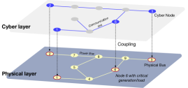
Figure 1: A depiction of cyber and physical topologies for CPPSs, with four critical cyber nodes and nine physical buses.

Though all physical layer nodes can be mapped to the cyber layer, at a minimum, the selection of critical cyber nodes should ensure the direct control of critical physical assets (e.g., generators). This allows lower costs on cyber resource deployment and flexibility on reconfiguring the cyber topology. As shown in Fig. 1, a set of predefined critical cyber nodes $K=\{1,2,3,6\}$ must be active and connected when constructing the cyber topology. Suppose cyber Node 6 is of high resilience priority due to the control of critical generation/load. On the compromise of Node 6, the cyber decision variable $\tilde{x}_{6}$ is used to decide whether to deploy another cyber resource and control of physical resources at Bus 6. For example, deploying an additional cyber resource while enabling a backup physical resource, such as a backup energy storage system (ESS), we have the cost objective of:

$$f_{\mathrm{res}}(\tilde{x}_{6},\bm{P}_{6}^{\mathrm{ess}})\coloneqq\tilde{c}^{\prime}_{6}\cdot\tilde{x}_{6}+(c_{6}^{\mathrm{ess}}+f_{\mathrm{ESS}}(\bm{P}_{6}^{\mathrm{ess}}))\cdot\tilde{x}_{6}$$ (12)

where $c_{6}^{\mathrm{ess}}$ denotes the startup cost of the backup ESS at Node 6, $\bm{P}_{6}^{\mathrm{ess}}\in\mathbb{R}^{T}$ denotes the charging/discharging profiles of the ESS across $T$ time intervals, and $f_{\mathrm{ESS}}(\cdot)$ can denote the ESS objective, e.g., battery degradation cost by $f_{\mathrm{ESS}}\coloneqq\|\bm{P}_{6}^{\mathrm{ess}}\|_{2}^{2}$. In return, the participation of a new ESS at the physical layer would require rescheduling of the physical side operation, enforcing new constraints on the ESS by:

$$\underline{P}_{i}^{\mathrm{ess}}\leq P_{i,t}^{\mathrm{ess}}\leq\overline{P}_{i}^{\mathrm{ess}},~\underline{e}_{i}\leq e_{i,t}^{\mathrm{ess}}\leq\overline{e}_{i}$$ (13)

where $e_{i,t}^{\mathrm{ess}}$ denotes the energy of the ESS at node $i$ at time $t$, $\underline{P}_{i}^{\mathrm{ess}}$ and $\overline{P}_{i}^{\mathrm{ess}}$ denote its lower and upper charging power limits, respectively, and $\underline{e}_{i}$ and $\overline{e}_{i}$ denote its lower and upper energy bounds, respectively.

III-C Cooperative Cyber-Physical Optimization

To ensure the optimal management of cyber and physical resources during power system contingencies, we develop the following resilient cyber-physical optimization model:

upper $$\min_{\mathscr{c}}\ \ \alpha_{1}f_{\mathrm{cyber}}$$ (14a)

$$\>\,\operatorname{s.t.}\ \ \eqref{flow_tree},\eqref{inoutflow_balance},\eqref{flow_limit},\eqref{activation_require}.$$ (14b)

lower $$\min_{\mathscr{p},\mathscr{r}}\ \ \alpha_{2}f_{\mathrm{power}}+\alpha_{3}f_{\mathrm{res}}$$ (14c)

$$\>\,\operatorname{s.t.}\ \ \eqref{eq_powerflow_full},\eqref{generator_limit},\eqref{voltage_limit},\eqref{ESS_individual_constraint}.$$ (14d)

where $\mathscr{c}=\{y_{\hat{\imath}\hat{\jmath}},\,x_{\hat{\imath}}\}$, $\mathscr{p}=\{\bm{P}_{i,g}^{\mathrm{gen}},\,\bm{Q}_{i,g}^{\mathrm{gen}}\}$, and $\mathscr{r}=\{\tilde{x}_{i},\bm{P}_{i}^{\mathrm{ess}}\}$ denote the sets of cyber, physical, and resilience variables, respectively, and $\alpha_{1}$, $\alpha_{1}$, and $\alpha_{3}$ are adjustable balancing coefficients. Problem (14) is framed as a bi-level optimization problem that incorporates both the cyber (upper) and cyber-physical (lower) layers into resilient CPPS operation.

To deploy the cooperative cyber-physical optimization model in (14), we propose an adaptive cyber and physical optimization algorithm shown in Algorithm 1.

Input: Cyber cost coefficients $c^{\prime}_{\hat{\imath}\hat{\jmath}}$, $c^{\prime}_{\hat{\imath}}$, $\tilde{c}^{\prime}_{\hat{\imath}}$, physical cost coefficients $c_{i,g}^{2}$, $c_{i,g}^{1}$, $c_{i,g}^{0}$, $c_{i}^{\mathrm{ess}}$, balancing coefficients $\alpha_{1}$, $\alpha_{1}$, $\alpha_{3}$, power system parameters.

Initialize: Solve (11) to initialize the cyber topology;

if Cyberattack is False then

    Solve (5) to control the physical resources based on the cyber topology;

   

else if Cyberattack is True then

    Isolate the corrupted cyber node $\hat{\imath}_{\tilde{c}}$;

    for Cyber sources $m\in\mathcal{M}_{\hat{\imath}_{\tilde{c}}}$ in parallel do

       Update the list of critical cyber nodes by replacing $\hat{\imath}_{\tilde{c}}$ with $m$;

       Solve (14a) and (14b) to find minimal cyber costs with $\tilde{x}_{6}$;

      

    end for

   Output updated cyber topology;

    Solve (14c) and (14d) to obtain physical actions in response to the cyberattack;

   

end if

Output: $\mathscr{c},\mathscr{p},\mathscr{r}$.

Algorithm 1 Adaptive cyber and physical resource optimization.

Algorithm 1 is suitable for cyber topology planning and providing response after cyber and/or physical attacks. In response to a cyber attack, the re-optimization allows cyber layer adaptively reroute the communication traffic by isolating the compromised cyber node(s) and updating the list of critical cyber nodes with minimal cyber costs. Afterwards, the physical power system is adjusted to utilize backup ESSs to return to an optimal operation status.

Remark 2

The cyber and physical layers can couple through both cooperative objectives (e.g., resilience goal) and competitive objectives (e.g., resource allocation cost). Problem (14) decouples the cyber and physical operation by designing a bi-level optimization problem. Note that the bi-level optimization problem doesnot ensure global optimality across both cyber and physical levels. Instead, it ensures optimality at both local cyber and physical levels while providing fast combined cyber and physical actions during cyber-physical contingencies. In this way, the bi-level solution also exemplifies the cyber-physical interactions through the allocation and control of cyber and physical resources. $\square$

IV Numerical Simulation

In the physical layer, consider the day-ahead power dispatch problem consisting of $T=12$ time steps with 2-hour intervals. The IEEE 14-bus test case is used as the test system, including 5 generators and loads connected to 11 buses (other than the slack bus and PV buses) [13, 14]. Bus 0 serves as the slack bus and maintains a normalized voltage magnitude of $V_{0}$. The upper and lower voltage magnitudes are set to be $\overline{V}=1.06V_{0}$ and $\underline{V}=0.94V_{0}$, respectively. The generator’s cost coefficients $c_{i,g}^{2}$, $c_{i,g}^{1}$, $c_{i,g}^{0}$ are set based on [14]. In the cyber layer, we map all physical buses into the cyber layer to obtain a potential list of cyber nodes based on the physical network topology. Then, the communication network consists of a single control center and certain substations, where the routers at the substation are denoted as critical cyber nodes that can control the cyber and physical assets within the area [15]. A set of generator nodes $\{1,2,3,6,8\}$ is initiated as critical cyber nodes that need to be connected. Node 1 is assumed to be the control center. All critical cyber nodes should be able to communicate with others. The cost coefficient for activating a cyber communication link can be referenced to the IEEE cost of Ethernet paths for the spanning tree [11]. We use solver IPOPT [16] to solve the optimization problem.

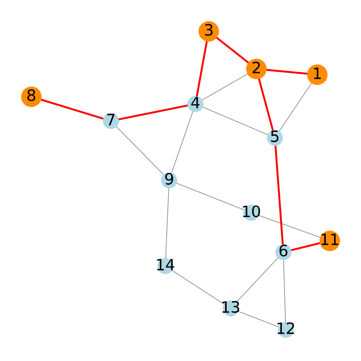
(a) Original cyber topology with Node 1 as the root node (before attack).

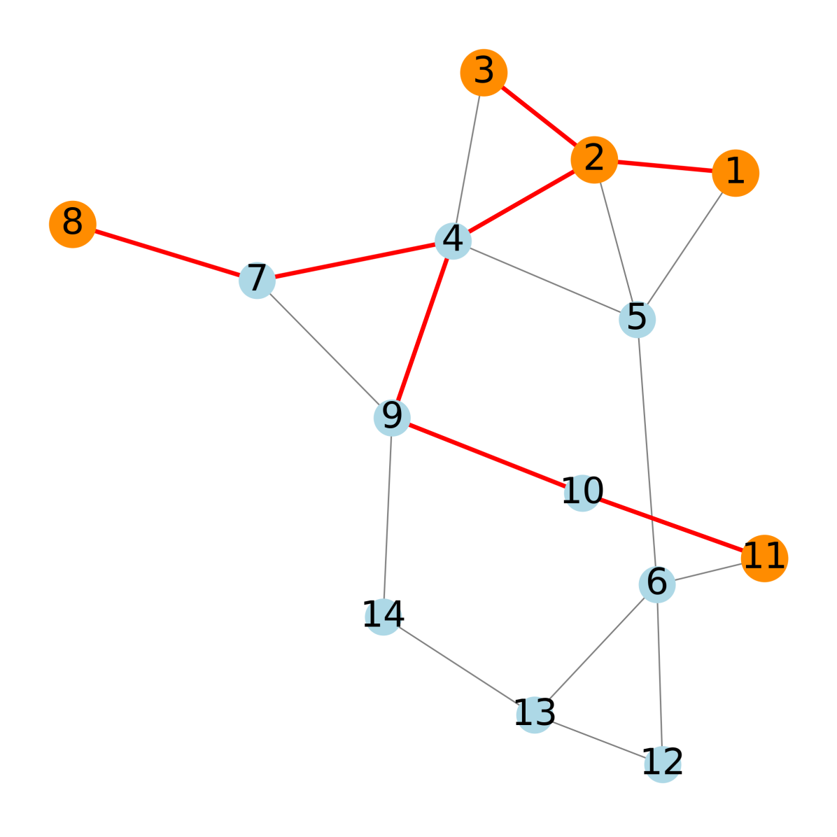
(b) Rerouted cyber topology (after attack).

Figure 2: Construction of cyber communication networks (black solid lines denote the physical power lines, critical cyber nodes are colored in orange).

Assume a combined cyber-physical attack that happens at 12:00, i.e., at time instance 6 that breaks one day into two equal length of periods. The cyber resource $x_{6}$ is attacked and needs to be isolated, and the generator $P_{6,g}^{\mathrm{gen}}$ at bus 6 is assumed to be out of operation caused by a physical disruption. Fig. 2(b) shows the reconfiguration of a cyber communication network after isolating Node 6. A set of neighboring cyber nodes $\mathcal{M}_{\tilde{6}}=\{11,12,13\}$ are candidates for replacing the cyber resource $x_{6}$. Following Algorithm 1, the neighboring cyber Node 11 is selected with minimal costs to reroute the cyber network. Subsequently, Node 11 controls the physical resources of bus 6, such as controlling or starting the ESS at bus 6. Fig. 3 shows the

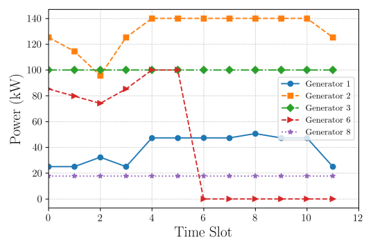
Figure 3: Active power generation of all generators after the cyber-physical attack.

shows the generators’ generations after the cyber-physical attack. As can be seen, Generator 6 stops functioning after time slot 6 with no active power generation. In Fig. 4,

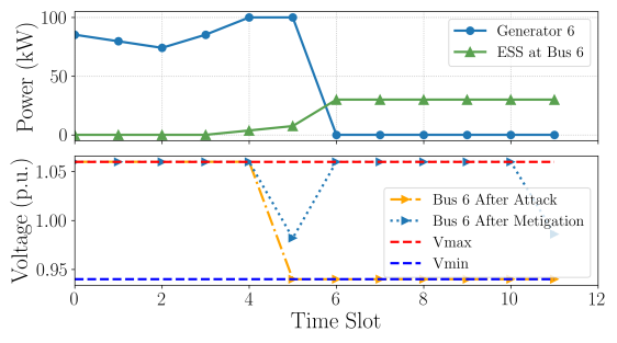
Figure 4: Active charging/discharging power of the ESS, and voltage magnitude of Bus 6 (before and after mitigation).

the upper figure shows that the ESS at Bus 6 starts to power the physical systems after the attack. The lower figure shows that the voltage magnitude of Bus 6 drops quickly after the attack, and the mitigation is effective in regulating the voltage to stay within the voltage limits.

V Conclusion and Future Work

In this paper, we present a synthesized cyber-physical resource optimization framework that cooperatively controls the cyber and physical resources within the power systems. By formulating the problem as a constrained optimization problem with cyber, physical, and cyber-physical objectives and constraints, we develop bi-level solutions to optimize the operation of cyber communication networks and physical power resources. The proposed method enhances grid resilience by cooperating the cyber and physical side actions, with adaptive response to cyber-physical contingencies. Numerical simulations on the modified IEEE 14-bus system validate the effectiveness of our approach, demonstrating its potential for the integrated control of grid-edge cyber and physical resources. Future work includes scaling up the solution to the large-scale cyber topology.

References

- [1] K. R. Davis, C. M. Davis, S. A. Zonouz, R. B. Bobba, R. Berthier, L. Garcia, and P. W. Sauer, “A cyber-physical modeling and assessment framework for power grid infrastructures,” IEEE Trans. Smart Grid, vol. 6, no. 5, pp. 2464–2475, 2015.
- [2] T. Li, B. Sun, Y. Chen, Z. Ye, S. H. Low, and A. Wierman, “Learning-based predictive control via real-time aggregate flexibility,” IEEE Trans. Smart Grid, vol. 12, no. 6, pp. 4897–4913, 2021.
- [3] X. Huo, H. Huang, K. R. Davis, H. V. Poor, and M. Liu, “A review of scalable and privacy-preserving multi-agent frameworks for distributed energy resources,” Adv. Appl. Energy, p. 100205, 2024.
- [4] M. Mahzarnia, M. P. Moghaddam, P. T. Baboli, and P. Siano, “A review of the measures to enhance power systems resilience,” IEEE Syst. J, vol. 14, no. 3, pp. 4059–4070, 2020.
- [5] M. F. Fard, X. Huo, and M. Liu, “Exploration of for-purpose decentralized algorithmic cyber attacks in EV charging control,” in Proc. 32nd Int. Symp. Ind. Electron., Helsinki, Finland, Jun. 19-21 2023, pp. 1–6.
- [6] A. Sahu, P. Wlazlo, N. Gaudet, A. Goulart, E. Rogers, and K. Davis, “Generation of firewall configurations for a large scale synthetic power system,” in Proc. IEEE Tex. Power Energy Conf., College Station, TX, USA, Feb. 28-Mar. 01 2022, pp. 1–6.
- [7] A. Rostami, M. Mohammadi, and H. Karimipour, “Reliability assessment of cyber-physical power systems considering the impact of predicted cyber vulnerabilities,” Int. J. Electr. Power Energy Syst., vol. 147, p. 108892, 2023.
- [8] K. Lai, M. Illindala, and K. Subramaniam, “A tri-level optimization model to mitigate coordinated attacks on electric power systems in a cyber-physical environment,” Appl. Energy, vol. 235, pp. 204–218, 2019.
- [9] T. R. B. Kushal and M. S. Illindala, “Decision support framework for resilience-oriented cost-effective distributed generation expansion in power systems,” IEEE Trans. Ind. Appl., vol. 57, no. 2, pp. 1246–1254, 2020.
- [10] M. B. Cain, R. P. O’neill, A. Castillo et al., “History of optimal power flow and formulations,” FERC, vol. 1, pp. 1–36, 2012.
- [11] “Spanning Tree Protocols.” [Online]. Available: https://www.ieee802.org/1/files/public/docs2009/aq-seaman-merged-spanning-tree-protocols-0509.pdf
- [12] R. Liu, C. Vellaithurai, S. S. Biswas, T. T. Gamage, and A. K. Srivastava, “Analyzing the cyber-physical impact of cyber events on the power grid,” IEEE Trans. Smart Grid, vol. 6, no. 5, pp. 2444–2453, 2015.
- [13] Illinois Information Trust Institute, “IEEE 14-bus system.” [Online]. Available: https://icseg.iti.illinois.edu/ieee-14-bus-system/
- [14] Matpower, “CASE14 power flow data for IEEE 14 bus test case.” [Online]. Available: https://matpower.org/docs/ref/matpower5.0/case14.html
- [15] M. R. Narimani, H. Huang, A. Umunnakwe, Z. Mao, A. Sahu, S. Zonouz, and K. Davis, “Generalized contingency analysis based on graph theory and line outage distribution factor,” IEEE Syst. J., vol. 16, no. 1, pp. 626–636, 2021.
- [16] L. T. Biegler and V. M. Zavala, “Large-scale nonlinear programming using IPOPT: An integrating framework for enterprise-wide dynamic optimization,” Comput. Chem. Eng., vol. 33, no. 3, pp. 575–582, 2009.