Mixed Quantum–Classical Dynamics Yields Anharmonic Rabi Oscillations

Abstract

We apply a mixed quantum–classical (MQC) approach to the quantum Rabi model, involving a classical optical field coupled self-consistently to a quantum two-level system. Under the rotating wave approximation, we analytically show this approach to yield persistent yet anharmonic Rabi oscillations, governed by an undamped and unforced Duffing equation. We consider the single-quantum limit, where we find such anharmonic Rabi oscillations to closely follow full-quantum results once zero-point energy is approximately enforced when initializing the optical field coordinate. Our findings provide guidance in the application of MQC dynamics to classes of problems involving small quantum numbers and far away from decoherence.

I Introduction

Mixed quantum–classical (MQC) dynamics offers a powerful framework for the simulation and interpretation of a wide range of phenomena. Throughout the last few decades, MQC dynamics has established itself as a preferred approach for the low-cost simulation of molecular systems, wherein nuclear motion is represented by classical coordinates while a quantum treatment is reserved for the electronic states C. Tully (1998); Nelson et al. (2014); Subotnik et al. (2016); Wang, Akimov, and Prezhdo (2016); Curchod and Martínez (2018); Crespo-Otero and Barbatti (2018). In recent years, it has been similarly employed for the modeling of materials Nie et al. (2014); Smith and Akimov (2019); Jiang et al. (2021); Lively et al. (2024); Krotz and Tempelaar (2024) and condensed-phase correlated phenomena Petrović, Weber, and Freericks (2024).

Although MQC dynamics is commonly found to provide accurate, or at least predictive, results, its realm of applicability remains poorly understood. According to the Bohr correspondence principle Bohr (1920), the classical approximation taken within MQC dynamics is justified so long as the relevant coordinates attain large quantum numbers. However, MQC dynamics has been shown to reach high accuracy even in cases where this criterion is grossly violated Tempelaar and Reichman (2017); Bondarenko and Tempelaar (2023). Such favorable performance may be explained based on the quasiclassical dynamics literature, where it has been shown that classical equations of motion approach quantum dynamics for harmonic potentials and in the short-time limit Heller (1981); Herman and Kluk (1984); Kay (2006). Yet, counterintuitive behaviors may arise once quantum and classical equations of motion are combined within a same framework, as famously exemplified by the Schrödinger cat thought experiment Schrödinger (1935). As an alternative, one may therefore resort to decoherence as a criterion for the applicability of MQC dynamics, meaning that the quantum–classical correlations should remain limited.

While most applications of MQC dynamics involve electron–nuclear coupling, light–matter interactions provide a complementary realm of applicability Sakko, Rossi, and Nieminen (2014); Ruggenthaler et al. (2018); Hoffmann et al. (2019a, b, 2020); Hsieh, Krotz, and Tempelaar (2023a, b); Weight, Li, and Zhang (2023). Notably, the canonical Rabi model, involving a two-level system (TLS) interacting with a single optical mode, was originally proposed within a MQC treatment, invoking a classical approximation for the mode Rabi (1937). While originally investigated under high field intensities and with neglect of feedback of the TLS onto the mode, a fully self-consistent treatment has since been explored A. Cives-esclop and Sánchez-Soto (1999), as well as behaviors in the quantum–classical crossover region Twyeffort Irish and Armour (2022). However, rapid advances in the areas of quantum optics Reiserer and Rempe (2015) and cavity quantum electrodynamics Ebbesen (2016); Ribeiro et al. (2018); Baranov et al. (2018); Hertzog et al. (2019); Hirai, Hutchison, and Uji-i (2020); Dunkelberger et al. (2022); Mandal et al. (2023); Xiang and Xiong (2024) have generated a particular interest in phenomena where field intensities approach the single-photon limit, as governed by the quantum Rabi model. Much remains to be learned about the applicability of MQC dynamics in this limit, and the ability of the quantum Rabi model to expose general guiding principles for MQC modeling.

In this Article, we apply MQC dynamics to the quantum Rabi model, specifically considering a TLS in its excited state interacting with a single resonant optical mode prepared in its ground state. When represented fully quantum-mechanically, this model is known to exhibit Rabi oscillations manifested as harmonic population fluctuations of the TLS Allen and Eberly (2012). As we show analytically within the rotating wave approximation (RWA), upon adopting a classical representation for the optical mode, Rabi oscillatory motion is instead governed by an undamped and unforced Duffing equation Duffing (1918). This equation involves an anharmonic term contributing a “mode softening effect” to the Rabi oscillations. The solutions to this equation are found to follow the quantum results closely upon (approximately) reinforcing zero-point energy when initializing the classical coordinate. These findings inform on the application of MQC dynamics to coherent phenomena involving small quantum numbers.

II Full-quantum representation

Before turning to MQC dynamics, we begin by briefly revisiting the quantum Rabi model within a full-quantum representation. For simplicity, we restrict ourselves to the scenario where the transition energy of the TLS is perfectly resonant with the optical mode. A schematic of this scenario is depicted in Fig. 1. Setting $\hbar=1$, and taking $\Omega$ to denote the TLS transition energy as well as the optical mode frequency, the corresponding Hamiltonian is given by

$$\hat{H}=\frac{1}{2}\left(\hat{p}^{2}+\Omega^{2}\hat{q}^{2}\right)+\Omega\ket{\phi_{\mathrm{e}}}\bra{\phi_{\mathrm{e}}}+\mu\Omega\lambda\hat{q}\left(\ket{\phi_{\mathrm{e}}}\bra{\phi_{\mathrm{g}}}+\mathrm{H.c.}\right).$$ (1)

Here, $\hat{q}$ and $\hat{p}$ are coordinate-like operators representing the optical mode, $\ket{\phi_{\mathrm{g}}}$ and $\ket{\phi_{\mathrm{e}}}$ refer to the ground and excited state of the TLS, $\mu$ is the associated transition dipole, $\lambda$ denotes the coupling strength between the TLS and the mode, and H.c. is short for Hermitian conjugate.

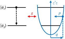
Figure 1: Schematic of the Rabi model. Shown are the ground and excited states of a two-level system (TLS), denoted $\ket{\phi_{\mathrm{g}}}$ and $\ket{\phi_{\mathrm{e}}}$, respectively. Also shown are the lowest two quantum levels of an optical mode, superimposed on a classical harmonic oscillator depiction, involving position and momentum coordinates $q$ and $p$, respectively. The classical optical occupancy, $z^{*}z$, is indicated. The coupling between the TLS and the optical mode is denoted as $g$.

The quantum Rabi Hamiltonian, Eq. 1, is commonly formulated by expressing the TLS in terms of Pauli spin matrices. We refrain from doing so, and instead adopt a ground- and excited-state notation, in order to simplify the forthcoming analysis, and to enforce a connection to quantum optics and quantum electrodynamics where the TLS commonly represents the lowest two states of an atom or other quantum emitter. In both research areas, optical phenomena commonly reach the single-quantum limit, while being amenable to the RWA. Under these conditions, Eq. 1 can be simplified by first expanding the position-like operator $\hat{q}$ into the optical ladder operators,

$$\hat{q}=\sqrt{\frac{1}{2\Omega}}\left(\hat{b}^{\dagger}+\hat{b}\right),$$ (2)

and by introducing the effective coupling constant $g\equiv\mu\lambda\sqrt{\Omega/2}$ (see Fig. 1). Application of the RWA, which relies on $\Omega\gg g$, then yields a single-quantum Jaynes–Cummings (JC) Hamiltonian Jaynes and Cummings (1963); Shore and Knight (1993) of the form

$$\hat{H}=\bar{\epsilon}+g\left(\ket{\phi_{\mathrm{e}}}\bra{\phi_{\gamma}}+\mathrm{H.c.}\right).$$ (3)

Here, $\ket{\phi_{\mathrm{e}}}$ implicitly assumes the optical mode to reside in its ground state, $\ket{0}$. The state $\ket{\phi_{\gamma}}$, on the other hand, denotes the first excitation of the optical mode, i.e., $\hat{b}^{\dagger}\ket{0}$, with the TLS in its ground state. Both $\ket{\phi_{\mathrm{e}}}$ and $\ket{\phi_{\gamma}}$ are degenerate and have an energy $\bar{\epsilon}=\frac{3}{2}\Omega$, with contributions $\Omega$ and $\frac{1}{2}\Omega$ due to the single quantum and the optical mode’s zero-point energy, respectively.

Upon an initialization of the TLS in state $\ket{\phi_{\mathrm{e}}}$, coherent energy exchange will ensue in the form of Rabi oscillations, manifested in the transient quantum populations. For state $\ket{\phi_{\mathrm{e}}}$, the population is given by $P_{\mathrm{e}}=|c_{\mathrm{e}}|^{2}$, with the wavefunction coefficient given by

$$c_{\mathrm{e}}=\Braket{\phi_{\mathrm{e}}|e^{-i\hat{H}t}|\phi_{\mathrm{e}}},$$ (4)

where $t$ denotes the time elapsed after initiation. This coefficient can be evaluated straightforwardly within the eigenbasis of the JC Hamiltonian, Eq. 3, with eigenvectors given by

$$\ket{\psi_{\pm}}=\frac{1}{\sqrt{2}}\left(\ket{\phi_{\mathrm{e}}}\pm\ket{\phi_{\gamma}}\right),$$ (5)

and with corresponding eigenenergies $\epsilon_{\pm}=\bar{\epsilon}\pm g$. It follows that

$$c_{\mathrm{e}} =\frac{1}{2}\left(\Braket{\psi_{+}|e^{-i\epsilon_{+}t}|\psi_{+}}+\Braket{\psi_{-}|e^{-i\epsilon_{-}t}|\psi_{-}}\right)$$

$$=e^{-i\bar{\epsilon}t}\cos(gt),$$ (6)

yielding

$$P_{\mathrm{e}}=\frac{1}{2}+\frac{1}{2}\cos\left(2gt\right),$$ (7)

which exposes Rabi oscillations at a frequency of $2g$.

Upon a replacement of the optical mode by a classical oscillator, Rabi oscillations can no longer be conveniently evaluated in the eigenbasis of the quantum Hamiltonian, and are to be evaluated in the physical basis instead. In order to contrast the resulting approach with that taken for the full-quantum representation, it is worth re-evaluating the latter within the physical basis. We reiterate that a formulation of the quantum Rabi Hamiltonian in terms of the TLS ground and excited states, rather than Pauli matrices, provides notational convenience in this evaluation, especially when we restrict ourselves to pure states of the TLS. In this case, we can describe the TLS in terms of the wavefunction

$$\ket{\Psi}=c_{\mathrm{e}}\ket{\phi_{\mathrm{e}}}+c_{\gamma}\ket{\phi_{\gamma}},$$ (8)

whose evolution is governed by the time-dependent Schrödinger equation, $i\ket{\dot{\Psi}}=\hat{H}\ket{\Psi}$. This yields dynamical equations for the wavefunction coefficients given by

$$\dot{c}_{\mathrm{e}}=-i\bar{\epsilon}c_{\mathrm{e}}-igc_{\gamma},\qquad\dot{c}_{\gamma}=-i\bar{\epsilon}c_{\gamma}-igc_{\mathrm{e}}.$$ (9)

When $\bar{\epsilon}\gg g$ (which is equivalent to $\Omega\gg g$), the evolution of the wavefunction coefficients will be dominated by phase oscillations at a frequency $\bar{\epsilon}$, due to the diagonal contributions to Eq. 9. Notably, these phase oscillations do not contribute to the population dynamics, which is instead dominated by a slower dynamical component. For that reason, it proves convenient to extract this component by dividing out the phase oscillations. Accordingly, we take

$$c_{\mathrm{e}}=\tilde{c}_{\mathrm{e}}e^{-i\bar{\epsilon}t},\qquad c_{\gamma}=\tilde{c}_{\gamma}e^{-i\bar{\epsilon}t},$$ (10)

where the slower component is denoted with a tilde. We note that, in principle, this decomposition can be performed even when $\bar{\epsilon}\gg g$ is violated. By application of the product rule for differentiation, it follows that

$$\dot{c}_{\mathrm{e}}=\dot{\tilde{c}}_{\mathrm{e}}e^{-i\bar{\epsilon}t}-i\bar{\epsilon}\tilde{c}_{\mathrm{e}}e^{-i\bar{\epsilon}t},\qquad\dot{c}_{\gamma}=\dot{\tilde{c}}_{\gamma}e^{-i\bar{\epsilon}t}-i\bar{\epsilon}\tilde{c}_{\gamma}e^{-i\bar{\epsilon}t}.$$ (11)

Combining Eqs. 9-11 yields

$$\dot{\tilde{c}}_{\mathrm{e}}=-ig\tilde{c}_{\gamma},\qquad\dot{\tilde{c}}_{\gamma}=-ig\tilde{c}_{\mathrm{e}},$$ (12)

upon which we find

$$\ddot{\tilde{c}}_{\mathrm{e}}=-g^{2}\tilde{c}_{\mathrm{e}}.$$ (13)

Under the initial conditions $\tilde{c}_{\mathrm{e}}=1$ and $\dot{\tilde{c}}_{\mathrm{e}}=0$, this is solved by $\tilde{c}_{\mathrm{e}}=\cos(gt)$, from which the transient excited-state population of the TLS follows as

$$P_{\mathrm{e}}=\tilde{c}_{\mathrm{e}}^{2}=\frac{1}{2}+\frac{1}{2}\cos\left(2gt\right),$$ (14)

in agreement with Eq. 7.

III Mixed quantum–classical representation

We now proceed by taking the classical approximation for the optical mode, starting from the quantum Rabi model. Accordingly, we replace the coordinate-like operators by their classical canonical coordinates in Eq. 1, i.e., $\hat{p}\rightarrow p$ and $\hat{q}\rightarrow q$. This substitution yields a MQC Rabi model, in which the the optical mode is represented by a classical harmonic oscillator, as depicted in Fig. 1. In the following, it proves convenient to represent the optical mode by means of a complex-valued classical coordinate defined as Krotz, Provazza, and Tempelaar (2021); Miyazaki, Krotz, and Tempelaar (2024)

$$z\equiv\sqrt{\frac{\Omega}{2}}\left(q+i\frac{p}{\Omega}\right).$$ (15)

Accordingly, the MQC Rabi Hamiltonian takes the form

$$\hat{H}=\Omega z^{*}z+\Omega\ket{\phi_{\mathrm{e}}}\bra{\phi_{\mathrm{e}}}+g\left(z^{*}+z\right)\left(\ket{\phi_{\mathrm{e}}}\bra{\phi_{\mathrm{g}}}+\mathrm{H.c.}\right).$$ (16)

We will now follow an approach similarly to that presented above for the full-quantum representation in the physical basis. As such, this approach differs from that taken previously for the MQC Rabi model based on Pauli matrices A. Cives-esclop and Sánchez-Soto (1999), and even though we sacrifice notational generalizability to mixed states, it simplifies the analysis considerably. First, the dynamical equations for the wavefunction coefficients take the form

$$\dot{c}_{\mathrm{e}} =-i(n+1)\Omega c_{\mathrm{e}}-ig\left(z^{*}+z\right)c_{\mathrm{g}},$$

$$\dot{c}_{\mathrm{g}} =-in\Omega c_{\mathrm{g}}-ig\left(z^{*}+z\right)c_{\mathrm{e}},$$ (17)

where we introduced the (classical) optical occupancy $n\equiv z^{*}z$, which is representative of the optical field intensity.

As before, it proves convenient to divide out the phase oscillations from the wavefunction coefficients. However, according to Eq. 17, the frequency of these phase oscillations is now dependent on $n$, which itself evolves in time. Accordingly, we take

$$c_{\mathrm{e}}=\tilde{c}_{\mathrm{e}}e^{-i\Omega\int n\;\mathrm{d}t}e^{-i\Omega t},\qquad c_{\mathrm{g}}=\tilde{c}_{\mathrm{g}}e^{-i\Omega\int n\;\mathrm{d}t},$$ (18)

where the integrals in the exponent are taken over the interval from initiation to the time at which the wavefunction coefficients are being evaluated. The equivalent of Eq. 11 now becomes

$$\dot{c}_{\mathrm{e}} =\dot{\tilde{c}}_{\mathrm{e}}e^{-i\Omega\int n\;\mathrm{d}t}e^{-i\Omega t}-i(n+1)\Omega c_{\mathrm{e}},$$

$$\dot{c}_{\mathrm{g}} =\dot{\tilde{c}}_{\mathrm{g}}e^{-i\Omega\int n\;\mathrm{d}t}-in\Omega c_{\mathrm{g}}.$$ (19)

Combining Eqs. 17-19 yields

$$\dot{\tilde{c}}_{\mathrm{e}}e^{-i\Omega t} =-ig\left(z^{*}+z\right)\tilde{c}_{\mathrm{g}},$$

$$\dot{\tilde{c}}_{\mathrm{g}} =-ig\left(z^{*}+z\right)\tilde{c}_{\mathrm{e}}e^{-i\Omega t}.$$ (20)

Our goal is to reformulate Eq. 20 into a single, closed-form equation for $\tilde{c}_{\mathrm{e}}$, similarly to Eq. 13 for the full-quantum case. To this end, we need to eliminate $z$ and $\tilde{c}_{\mathrm{g}}$. We first recognize that the dynamics of $z$ is governed by Miyazaki, Krotz, and Tempelaar (2024)

$$\dot{z}=-i\frac{\partial H}{\partial z^{*}}.$$ (21)

Adopting the Ehrenfest theorem Ehrenfest (1927), the classical Hamiltonian follows from the quantum Hamiltonian as

$$H =\braket{\Psi|\hat{H}|\Psi}$$

$$=\Omega z^{*}z+\Omega\tilde{c}_{\mathrm{e}}^{*}\tilde{c}_{\mathrm{e}}+g(z^{*}+z)\left(c_{\mathrm{e}}^{*}c_{\mathrm{g}}+\mathrm{H.c.}\right).$$ (22)

This yields

$$\dot{z}=-i\Omega z-ig\left(c_{\mathrm{e}}^{*}c_{\mathrm{g}}+\mathrm{H.c.}\right).$$ (23)

Similarly as for the wavefunction coefficients, it proves convenient to divide phase oscillations out of $z$, according to

$$z=\tilde{z}e^{-i\Omega t}.$$ (24)

Substitution into Eq. 20 yields

$$\dot{\tilde{c}}_{\mathrm{e}}=-ig\tilde{z}\tilde{c}_{\mathrm{g}},\qquad\dot{\tilde{c}}_{\mathrm{g}}=-ig\tilde{z}^{*}\tilde{c}_{\mathrm{e}},$$ (25)

where we adopted the RWA as we did for the quantum Rabi model. From this, it follows that

$$\ddot{\tilde{c}}_{\mathrm{e}} =-ig(\tilde{z}\dot{\tilde{c}}_{\mathrm{g}}+\dot{\tilde{z}}\tilde{c}_{\mathrm{g}})$$

$$=-g^{2}n\tilde{c}_{\mathrm{e}}-ig\dot{\tilde{z}}\tilde{c}_{\mathrm{g}},$$ (26)

where we used that the optical occupancy can be expressed as $n=\tilde{z}^{*}\tilde{z}$.

Evaluation of $\dot{\tilde{z}}$ proceeds in the same way as for the wavefunction coefficients. Accordingly, we first recognize that

$$\dot{z}=\dot{\tilde{z}}e^{-i\Omega t}-i\Omega z,$$ (27)

which combined with Eqs. 19 and 23 yields

$$\dot{\tilde{z}}=-ig\tilde{c}_{\mathrm{g}}^{*}\tilde{c}_{\mathrm{e}}.$$ (28)

Substitution into Eq. 26 results in

$$\ddot{\tilde{c}}_{\mathrm{e}}=-g^{2}\left(1+n-\tilde{c}_{\mathrm{e}}^{*}\tilde{c}_{\mathrm{e}}\right)\tilde{c}_{\mathrm{e}},$$ (29)

where we employed the normalization condition $\tilde{c}_{\mathrm{e}}^{*}\tilde{c}_{\mathrm{e}}+\tilde{c}_{\mathrm{g}}^{*}\tilde{c}_{\mathrm{g}}=1$ in order to eliminate $\tilde{c}_{\mathrm{g}}^{*}\tilde{c}_{\mathrm{g}}$.

So long as $\Omega\gg g$ is satisfied, the total combined energy of the TLS and the optical field is well approximated as $E=N\Omega$, with $N=\left(n+\tilde{c}_{\mathrm{e}}^{*}\tilde{c}_{\mathrm{e}}\right)$ representing the sum of the TLS and the optical occupancies. Since $E$ is a conserved quantity, so is $N$. If we initialize the TLS in its excited state, i.e., $\tilde{c}_{\mathrm{e}}=1$, and denote the initial optical occupancy as $n_{0}$, we thus have that $n+\tilde{c}_{\mathrm{e}}^{2}=n_{0}+1$. Moreover, if $\tilde{c}_{\mathrm{e}}$ initializes as real-valued, it will remain real-valued throughout the dynamics. Consequently, Eq. 29 simplifies to

$$\ddot{\tilde{c}}_{\mathrm{e}}=-\left(2+n_{0}\right)g^{2}\tilde{c}_{\mathrm{e}}+2g^{2}\tilde{c}_{\mathrm{e}}^{3}.$$ (30)

Eq. 30 takes the form of an undamped and unforced Duffing equation Duffing (1918), with a harmonic term $-(2+n_{0})g^{2}$ and with an anharmonic term $2g^{2}$. The Duffing equation is ubiquitous in many branches of physics and engineering, and has long been under scrutiny Kovacic and Brennan (2011); Cvetićanin (2013). Eq. 30 is generally solved in terms of Jacobi elliptic functions, with specific solutions dependent on the initial conditions taken. We note that insightful simplified forms of these solutions have remained out of reach. What is known, however, is that the solutions are periodic Abramowitz and Stegun (1968). As such, while the Duffing equation governing the population dynamics within the MQC Rabi model is markedly different from the quantum equivalent, Eq. 13, we find persistent oscillations to be retained, with oscillatory behavior dependent on the initial optical occupancy, $n_{0}$. Within this oscillatory motion, the anharmonic term in the Duffing equation exerts a “mode softening” effect.

There is a trivial limit for which a simple analytical solution to Eq. 30 is readily available, corresponding to $n_{0}=0$. In this limit, Eq. 30 reduces to $\ddot{\tilde{c}}_{\mathrm{e}}\approx 0$. If we reinforce $\dot{\tilde{c}}_{\mathrm{e}}=0$ as an initial condition, as before, we thus find a complete absence of dynamics in this limit. This result is consistent with the fundamental principle that spontaneous emission requires optical vacuum fluctuations to be incorporated Li et al. (2018). These are not automatically accounted for by classical coordinates, and vanish rigorously for $n_{0}=0$.

Incorporation of optical vacuum fluctuations thus require an initialization satisfying $n_{0}>0$. There are various possibilities in which this criterion can be satisfied. For now, however, we chose to remain agnostic to these possibilities, and instead proceed to systematically and numerically assess the effect of classical coordinate initialization on the MQC Rabi oscillations governed by Eq. 30. Notably, through the dependence of this equation on the initial optical occupancy, $n_{0}=z_{0}^{*}z_{0}$, these oscillations depend on the norm of the initial coordinate $z_{0}$, but not on its phase. This is a direct consequence of the condition $\Omega\gg g$, implying that phase oscillations are infinitely rapid compared to the coherent energy exchange between the TLS and the optical mode.

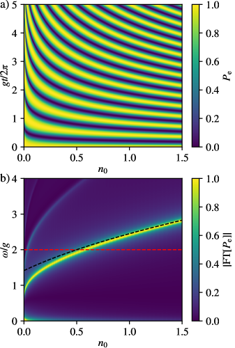
Figure 2: (a) Transient excited-state population of the two-level system (TLS), $P_{\mathrm{e}}=\tilde{c}_{\mathrm{e}}^{2}$, obtained from the solutions of the undamped and unforced Duffing equation, Eq. 30. Shown are results as a function of the initial optical occupancy, $n_{0}$. (b) Fourier transform of $P_{\mathrm{e}}$. Asymptotic frequency of the dominant harmonic given by Eq. 34 (black dash) and quantum Rabi oscillation at $\omega=2g$ (red dash) are indicated.

Shown in Fig. 2 (a) is the transient excited-state population of the TLS, $P_{\mathrm{e}}=\tilde{c}_{\mathrm{e}}^{2}$, obtained from the solutions to Eq. 30, as a function of $n_{0}$. As anticipated, clear periodic oscillations are observed. Evidently, the oscillation frequency is proportional to $n_{0}$, suggesting that the lack of dynamics in the limit $n_{0}\rightarrow 0$ can be understood as an oscillation with infinite periodicity. The frequency trend is further elucidated in Fig. 2 (b), showing the Fourier transform of $P_{\mathrm{e}}$ as a function of frequency, $\omega$, and initial optical occupancy, $n_{0}$. For each $n_{0}$, the Fourier transform was performed over a duration of $gt=200$, after multiplication of $P_{\mathrm{e}}$ by an exponential with an $1/e$ time of $gt=20$ to avoid clipping and after subtracting a 0.5 baseline, upon which the signal was normalized to the maximum peak. A dominant oscillatory component is observable alongside several minor components that vanish as $n_{0}$ increases. This is suggestive of harmonic oscillatory motion being recovered for $n_{0}\gg 0$. This limit turns out to be amenable to an approximate analytical treatment, providing deeper insights into MQC Rabi oscillations.

Accordingly, we first recognize that for $n_{0}\gg 0$ the anharmonic term will provide only a minor contribution to Eq. 30. As a result, we may expect the solution to this equation to be well-represented by the ansatz $\tilde{c}_{\mathrm{e}}=\cos(\tilde{\omega}t)$, where $\tilde{\omega}$ is the dominant harmonic that needs determining. Substituting this ansatz into Eq. 30 yields

$$-\tilde{\omega}^{2}\cos(\tilde{\omega}t) =-(2+n_{0})g^{2}\cos(\tilde{\omega}t)+\frac{3}{2}g^{2}\cos(\tilde{\omega}t)$$

$$\qquad+\frac{1}{2}g^{2}\cos(3\tilde{\omega}t),$$ (31)

where we used that

$$\cos^{3}(\tilde{\omega}t)=\frac{3}{4}\cos(\tilde{\omega}t)+\frac{1}{4}\cos(3\tilde{\omega}t).$$ (32)

The $\cos(3\tilde{\omega}t)$ term appearing on the right-hand side of Eq. 31 deserves a brief discussion. First, its prefactor is $\times 3$ smaller than that of the preceding term, which in turn is already a correction to the first term involving $n_{0}$. Hence, although our ansatz can be refined in order to include the $\cos(3\tilde{\omega}t)$ contribution, we expect resulting corrections to the dominant oscillation frequency to be minor. Instead, we proceed with Eq. 31 and balance only the $\cos(\tilde{\omega}t)$ terms. Doing so, and dividing by $\cos(\tilde{\omega}t)$, yields

$$\tilde{\omega}^{2}\approx\left(n_{0}+\frac{1}{2}\right)g^{2}.$$ (33)

The asymptotic Rabi oscillation frequency then follows as

$$\omega=2\tilde{\omega}\approx 2g\sqrt{n_{0}+1/2}.$$ (34)

This asymptote is indicated in Fig. 2, and the dominant component of the calculated MQC Rabi oscillation is seen to indeed approach this frequency with increasing $n_{0}$.

The asymptotic frequency given by Eq. 34 forms an interesting contrast with the known behavior of the Rabi model within a full-quantum treatment, for which we have $\omega=2g\sqrt{n_{0}+1}$ (with $n_{0}$ representing the quantum occupancy). Interestingly, the MQC Rabi model with neglect of feedback of the TLS on the classical optical field instead yields $\omega=2g\sqrt{n_{0}}$ Allen and Eberly (2012). As such, the self-consistent MQC Rabi model presented here emerges as an interesting “intermediate” between those limiting cases.

Another curious aspect of Eq. 34 pertains to the single-quantum limit. Here, Eq. 34 predicts $n_{0}=1/2$ to be the value for which MQC Rabi oscillations reproduce quantum Rabi oscillations at $\omega=2g$. For this occupancy, the classical field assumes an energy corresponding to that of vacuum fluctuations. This suggests that for MQC Rabi oscillations to reproduce the full-quantum result, the optical field needs to be initialized roughly at the zero-point energy. However, as seen in Fig. 2 (b), the dominant MQC Rabi component begins to undershoot Eq. 34 with decreasing occupancy, in order to satisfy $\omega\rightarrow 0$ for $n_{0}\rightarrow 0$. To offset this effect, MQC Rabi oscillations reproduce the quantum result (also indicated in Fig. 2 (b)) most closely at an occupancy exceeding the zero-point value, that is, at approximately $n_{0}=0.59$. This is evident from Fig. 2, where the quantum Rabi oscillation at $\omega=2g$ is indicated.

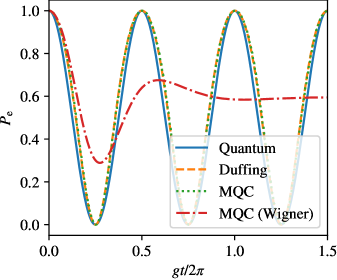
Figure 3: Excited-state population of the TLS, $P_{\mathrm{e}}=\tilde{c}_{\mathrm{e}}^{2}$, obtained from the solution to the undamped and unforced Duffing equation, Eq. 30, for $n_{0}=0.59$ (orange dash), compared with the full-quantum result (blue solid). Also shown are results from MQC dynamics under focused sampling (dotted) and under Wigner sampling (red dash-dotted), obtained using $\Omega=50$.

To assess how closely the MQC Rabi oscillation at $n_{0}=0.59$ follows the quantum result, we present in Fig. 3 a comparison of $P_{\mathrm{e}}=\tilde{c}_{\mathrm{e}}^{2}$ obtained from the Duffing equation, Eq. 30, with that from the quantum Rabi model, Eq. 7, as a function of time. As can be seen, both results are in broad agreement, with a matching dominant oscillation component. The mode-softening effect contained in the Duffing equation manifests as a population bias of the MQC Rabi oscillation towards the excited state of the TLS.

Fig. 3 includes MQC simulation results obtained by directly solving Eq. 16 for $n_{0}=0.59$. In these simulations, $\Omega=50g$ is taken in order to ensure that the RWA is applicable, and that the initial phase of the optical field does not affect the dynamics. The latter justifies an initialization of the classical coordinates at $p=0$ and $q>0$, and negates the need for trajectory sampling. The results coming out of this approach are in close agreement with those produced by the Duffing equation, Eq. 30, substantiating the validity of our analysis.

Our findings suggest that for the model at hand, MQC dynamics are best performed with an initialization of the classical coordinates with a well-defined energy lying slightly above the zero-point energy, by setting $n_{0}=0.59$. This contrasts with the approach commonly taken in MQC dynamics wherein classical coordinates are stochastically sampled from a Wigner quasi-probability distribution Wigner (1932), giving rise to a distribution of initial energies that average out to the zero-point energy. To further investigate this contrast, we have also included in Fig. 3 MQC simulation results where such Wigner sampling is conducted. Accordingly, $p$ and $q$ are stochastically drawn from the normal distribution

$$\Gamma(p,q)=\frac{1}{\pi}\mathrm{exp}\left(-\frac{p^{2}}{\Omega}-\Omega q^{2}\right),$$ (35)

while an average over 100 000 trajectories is taken, which proved necessary to ensure convergence. As is obvious from Fig. 3, such Wigner sampling performs poorly in reproducing the Rabi oscillations, yielding rapidly-decaying population dynamics instead of persistent oscillations. From Fig. 2, the rapid decay is attributed to Wigner sampling effectively taking an average over oscillatory dynamics with different $n_{0}$ values for which the distribution of frequencies is broad. In this process, $P_{\mathrm{e}}$ equilibrates to a value exceeding 0.5 in Fig. 3, attributable to the population bias towards the excited state of the TLS, resulting from the anharmonic term in the Duffing equation, Eq. 30.

The preference of enforcing $n_{0}$ to (roughly) match the zero-point energy, instead of Wigner sampling of trajectories, resonates with previous studies. At times referred to as “focused sampling”, such reinforcement of physical properties at the single-trajectory level Stock and Müller (1999) is commonly envisioned as a means to accelerate convergence with respect to the number of trajectories Bonella and Coker (2003); Bonella, Montemayor, and Coker (2005); Kim, Nassimi, and Kapral (2008) and has found applications in conjunction with various quasiclassical approaches Mandal, Yamijala, and Huo (2018); Runeson and Richardson (2019); Ananth (2022). Importantly, while focused sampling enables convergence at the single-trajectory level for the Rabi model studied here, its most essential effect is the remedying of unphysical behaviors arising under Wigner sampling. It should be noted that unphysical behaviors under Wigner sampling have been observed in previous studies Tempelaar and Reichman (2017); Bondarenko and Tempelaar (2023); Hsieh, Krotz, and Tempelaar (2023b).

IV Discussion

In summary, we have shown that Rabi oscillations can to a good approximation be reproduced by MQC dynamics, even in the single-quantum limit. The resulting population dynamics is governed by an undamped and unforced Duffing equation, Eq. 30, involving an anharmonic term, the solutions of which consist of persistent oscillatory functions with frequencies dependent on the initial occupancy of the optical mode. Rough agreement with the quantum result is found when this occupancy is initialized such that the zero-point energy is approximately enforced for the optical mode. These results underscore the advantage of so-called focused sampling techniques Stock and Müller (1999) in MQC dynamics over commonly-applied Wigner sampling. However, which approach is preferred may be highly susceptible to the problem at hand; something that is worthy of further inquiry.

As mentioned before, the quantum Rabi model has previously been subjected to a self-consistent MQC treatment such as presented here, but within a Pauli matrix representation A. Cives-esclop and Sánchez-Soto (1999). This analysis resulted in 5 coupled differential equations, upon which solutions could be derived in the form of Jacobi elliptic functions. As such, these solutions shows consistency with our Duffing equation analysis. We note that the corresponding dynamics was previously assessed exclusively for larger quantum numbers, for which the Jacobi elliptic functions become harmonic.

Here, we restricted ourselves to the scenario of a TLS interacting with a single optical mode. Previous studies have considered the performance of MQC dynamics under Wigner sampling to the scenario where the number of optical modes is large Hoffmann et al. (2019a, b); Saller, Kelly, and Geva (2021); Hsieh, Krotz, and Tempelaar (2023a, b). Under application of the Ehrenfest theorem, Eq. 22, this approach was shown to yield quantitative inaccuracies Hoffmann et al. (2019a, b); Saller, Kelly, and Geva (2021), and at times qualitative failures Hsieh, Krotz, and Tempelaar (2023a, b). These shortcomings are remedied by a recently-proposed scheme wherein optical vacuum fluctuations are selectively decoupled from the atomic ground state Hsieh, Krotz, and Tempelaar (2023a, b). It will thus be of interest to revisit such a “decoupled” Ehrenfest approach and incorporate the focused sampling scheme adopted in the present work, in order to deliver a MQC dynamics method providing optimal accuracy for both small and large mode numbers. Lastly, it is worth noting that the Rabi model bears similarities with other canonical scenarios, including the spin–boson model. As such, our findings may offer guidance to the application of MQC dynamics beyond the quantum Rabi model. Altogether, these efforts open new realms of accurate MQC modeling.

References

- C. Tully (1998) J. C. Tully, Faraday Discuss. 110, 407 (1998).
- Nelson et al. (2014) T. Nelson, S. Fernandez-Alberti, A. E. Roitberg, and S. Tretiak, Acc. Chem. Res. 47, 1155 (2014).
- Subotnik et al. (2016) J. E. Subotnik, A. Jain, B. Landry, A. Petit, W. Ouyang, and N. Bellonzi, Annu. Rev. Phys. Chem. 67, 387 (2016).
- Wang, Akimov, and Prezhdo (2016) L. Wang, A. Akimov, and O. V. Prezhdo, J. Phys. Chem. Lett. 7, 2100 (2016).
- Curchod and Martínez (2018) B. F. E. Curchod and T. J. Martínez, Chem. Rev. 118, 3305 (2018).
- Crespo-Otero and Barbatti (2018) R. Crespo-Otero and M. Barbatti, Chem. Rev. 118, 7026 (2018).
- Nie et al. (2014) Z. Nie, R. Long, L. Sun, C.-C. Huang, J. Zhang, Q. Xiong, D. W. Hewak, Z. Shen, O. V. Prezhdo, and Z.-H. Loh, ACS Nano 8, 10931 (2014).
- Smith and Akimov (2019) B. Smith and A. V. Akimov, J. Phys. Condens. Matter 32, 073001 (2019).
- Jiang et al. (2021) X. Jiang, Q. Zheng, Z. Lan, W. A. Saidi, X. Ren, and J. Zhao, Sci. Adv. 7, eabf3759 (2021).
- Lively et al. (2024) K. Lively, S. A. Sato, G. Albareda, A. Rubio, and A. Kelly, Phys. Rev. Res. 6, 013069 (2024).
- Krotz and Tempelaar (2024) A. Krotz and R. Tempelaar, J. Chem. Phys. 161, 044117 (2024).
- Petrović, Weber, and Freericks (2024) M. D. Petrović, M. Weber, and J. K. Freericks, Phys. Rev. X 14, 031052 (2024).
- Bohr (1920) N. Bohr, Z. Phys. 2, 423 (1920).
- Tempelaar and Reichman (2017) R. Tempelaar and D. R. Reichman, J. Chem. Phys. 148, 102309 (2017).
- Bondarenko and Tempelaar (2023) A. S. Bondarenko and R. Tempelaar, J. Chem. Phys. 158, 054117 (2023).
- Heller (1981) E. J. Heller, J. Chem. Phys. 75, 2923 (1981).
- Herman and Kluk (1984) M. F. Herman and E. Kluk, Chem. Phys. 91, 27 (1984).
- Kay (2006) K. G. Kay, Chem. Phys. 322, 3 (2006).
- Schrödinger (1935) E. Schrödinger, Sci. Nat. 23, 844 (1935).
- Sakko, Rossi, and Nieminen (2014) A. Sakko, T. P. Rossi, and R. M. Nieminen, J. Phys. Condens. Matter 26, 315013 (2014).
- Ruggenthaler et al. (2018) M. Ruggenthaler, N. Tancogne-Dejean, J. Flick, H. Appel, and A. Rubio, Nat. Rev. Chem. 2, 0118 (2018).
- Hoffmann et al. (2019a) N. M. Hoffmann, C. Schäfer, A. Rubio, A. Kelly, and H. Appel, Phys. Rev. A 99, 063819 (2019a).
- Hoffmann et al. (2019b) N. M. Hoffmann, C. Schäfer, N. Säkkinen, A. Rubio, H. Appel, and A. Kelly, J. Chem. Phys. 151, 244113 (2019b).
- Hoffmann et al. (2020) N. M. Hoffmann, L. Lacombe, A. Rubio, and N. T. Maitra, J. Chem. Phys. 153, 104103 (2020).
- Hsieh, Krotz, and Tempelaar (2023a) M.-H. Hsieh, A. Krotz, and R. Tempelaar, J. Phys. Chem. Lett. 14, 1253 (2023a).
- Hsieh, Krotz, and Tempelaar (2023b) M.-H. Hsieh, A. Krotz, and R. Tempelaar, J. Chem. Phys. 159, 221104 (2023b).
- Weight, Li, and Zhang (2023) B. M. Weight, X. Li, and Y. Zhang, Phys. Chem. Chem. Phys. 25, 31554 (2023).
- Rabi (1937) I. I. Rabi, Phys. Rev. 51, 652 (1937).
- A. Cives-esclop and Sánchez-Soto (1999) A. L. A. Cives-esclop and L. L. Sánchez-Soto, J. Mod. Opt. 46, 639 (1999).
- Twyeffort Irish and Armour (2022) E. K. Twyeffort Irish and A. D. Armour, Phys. Rev. Lett. 129, 183603 (2022).
- Reiserer and Rempe (2015) A. Reiserer and G. Rempe, Rev. Mod. Phys. 87, 1379 (2015).
- Ebbesen (2016) T. W. Ebbesen, Acc. Chem. Res. 49, 2403 (2016).
- Ribeiro et al. (2018) R. F. Ribeiro, L. A. Martínez-Martínez, M. Du, J. Campos-Gonzalez-Angulo, and J. Yuen-Zhou, Chem. Sci. 9, 6325 (2018).
- Baranov et al. (2018) D. G. Baranov, M. Wersäll, J. Cuadra, T. J. Antosiewicz, and T. Shegai, ACS Photonics 5, 24 (2018).
- Hertzog et al. (2019) M. Hertzog, M. Wang, J. Mony, and K. Börjesson, Chem. Soc. Rev. 48, 937 (2019).
- Hirai, Hutchison, and Uji-i (2020) K. Hirai, J. A. Hutchison, and H. Uji-i, ChemPlusChem 85, 1981 (2020).
- Dunkelberger et al. (2022) A. D. Dunkelberger, B. S. Simpkins, I. Vurgaftman, and J. C. Owrutsky, Annu. Rev. Phys. Chem. 73, 429 (2022).
- Mandal et al. (2023) A. Mandal, M. A. Taylor, B. M. Weight, E. R. Koessler, X. Li, and P. Huo, Chem. Rev. 123, 9786 (2023).
- Xiang and Xiong (2024) B. Xiang and W. Xiong, Chem. Rev. 124, 2512 (2024).
- Allen and Eberly (2012) L. Allen and J. H. Eberly, Optical resonance and two-level atoms (Courier Corporation, 2012).
- Duffing (1918) G. Duffing, Erzwungene Schwingungen bei veränderlicher Eigenfrequenz und ihre technische Bedeutung, 41-42 (Vieweg, 1918).
- Jaynes and Cummings (1963) E. Jaynes and F. Cummings, Proc. IEEE 51, 89 (1963).
- Shore and Knight (1993) B. W. Shore and P. L. Knight, J. Mod. Opt. 40, 1195 (1993).
- Note (1) We note that mixed states can always be evaluated by taking an average over pure-state trajectories.
- Note (2) Here, avoid the commonly used “semiclassical” denomination, in order to differentiate such treatment from that of a quasiclassical approach, for which similar terminology is oftentimes used.
- Krotz, Provazza, and Tempelaar (2021) A. Krotz, J. Provazza, and R. Tempelaar, J. Chem. Phys. 154, 224101 (2021).
- Miyazaki, Krotz, and Tempelaar (2024) K. Miyazaki, A. Krotz, and R. Tempelaar, J. Chem. Theory Comput. 20, 6500 (2024).
- Ehrenfest (1927) P. Ehrenfest, Z. Phys. 45, 455 (1927).
- Kovacic and Brennan (2011) I. Kovacic and M. J. Brennan, The Duffing equation: nonlinear oscillators and their behaviour (John Wiley & Sons, 2011).
- Cvetićanin (2013) L. Cvetićanin, Theoret. Appl. Mech. 40, 49 (2013).
- Abramowitz and Stegun (1968) M. Abramowitz and I. A. Stegun, Handbook of mathematical functions with formulas, graphs, and mathematical tables, Vol. 55 (US Government printing office, 1968).
- Li et al. (2018) T. E. Li, A. Nitzan, M. Sukharev, T. Martinez, H.-T. Chen, and J. E. Subotnik, Phys. Rev. A 97, 032105 (2018).
- Wigner (1932) E. Wigner, Phys. Rev. 40, 749 (1932).
- Stock and Müller (1999) G. Stock and U. Müller, J. Chem. Phys. 111, 65 (1999).
- Bonella and Coker (2003) S. Bonella and D. F. Coker, J. Chem. Phys. 118, 4370 (2003).
- Bonella, Montemayor, and Coker (2005) S. Bonella, D. Montemayor, and D. F. Coker, Proc. Natl. Acad. Sci. U.S.A. 102, 6715 (2005).
- Kim, Nassimi, and Kapral (2008) H. Kim, A. Nassimi, and R. Kapral, J. Chem. Phys. 129, 084102 (2008).
- Mandal, Yamijala, and Huo (2018) A. Mandal, S. S. Yamijala, and P. Huo, J. Chem. Theory Comput. 14, 1828 (2018).
- Runeson and Richardson (2019) J. E. Runeson and J. O. Richardson, J. Chem. Phys. 151, 044119 (2019).
- Ananth (2022) N. Ananth, Annu. Rev. Phys. Chem. 73, 299 (2022).
- Saller, Kelly, and Geva (2021) M. A. C. Saller, A. Kelly, and E. Geva, J. Phys. Chem. Lett. 12, 3163 (2021).