Microcausality without Lorentz invariance

Abstract

Microcausality—the vanishing of commutators outside the lightcone—is a fundamental property of relativistic quantum field theories. We derive its implications for two-point functions of scalar operators on Lorentz-breaking states. We restrict to spatially homogeneous and isotropic states, at zero and finite temperature, such as finite-density states of matter and primordial inflationary states. In a mixed $(t,\vec{k}\,)$ representation, we find certain analyticity and exponential boundedness conditions, which we verify in a variety of examples. Crucially, we discuss how our conditions can be tested within the regime of validity of Lorentz-breaking low-energy effective field theories, clarifying the role of the group velocity of low-energy excitations. In the cosmological case, we derive a positivity condition on an EFT coefficient in an inflationary background. Lastly, we comment on how microcausality can be used to constrain higher-point correlation functions, via suitable nested commutators.

1 Introduction

One of the defining properties of relativistic quantum field theories (QFT’s) is the fact that local observables commute at spacelike separations Strocchi ,

$$[{\cal O}_{1}(x),{\cal O}_{2}(y)]=0\qquad\mbox{if}\;(x-y)^{2}<0\;,$$ (1)

where ${\cal O}_{1}(x)$ and ${\cal O}_{2}(x)$ are any two bosonic, gauge-invariant local operators, and we are using the mostly-minus signature for the metric. This property goes under the name of microcausality.

As discussed at length in Dubovsky:2007ac , on the one hand microcausality is tied to Lorentz-invariance, but, on the other hand, since it is an operator statement, it must hold on all possible states of the theory, including Lorentz-breaking ones. Now, it so happens that the only Lorentz invariant state of a relativistic QFT is the vacuum. So, what are the implications of the above operator statement when we evaluate it on a state that is not the vacuum? The obvious answer is that certain correlation functions, in particular the retarded and advanced ones, must vanish outside the light-cone, regardless of the state of the system. In particular, for a generic state, such correlation functions will not be Lorentz-invariant, but they will still obey relativistic causality.

Such considerations were recently leveraged in Creminelli:2022onn ; Heller:2022ejw ; Creminelli:2024lhd in order to derive analytic properties of Fourier-space two-point functions in homogeneous and isotropic Lorentz-breaking states, with the goal of deriving sum rules and positivity bounds for the effective theories describing the low-energy physics of those states. Our approach and goal are similar, but we find it useful, as we will discuss, to consider correlation functions in a mixed $(t,\vec{k}\,)$ representation. This, among other things, has the advantage of allowing us to apply our results to cosmological correlators. Another advantage is that the analyticity and boundedness conditions in the mixed $(t,\vec{k}\,)$ representation are necessary and sufficient for microcausality, whereas analyticity of retarded correlators in $(\omega,\vec{k}\,)$ is only a necessary condition, unless supplemented by a different boundedness condition, as we will show.

In particular, we will consider generic spatially translationally and rotationally invariant states in a generic QFT that obeys microcausality. The states can be pure, such as the ground state of a superfluid, or mixed, such as the equilibrium, finite-temperature state of a normal fluid. We will never use Lorentz invariance—since our states break it—and so in a sense it is not even needed that the underlying QFT be Lorentz invariant, provided it obeys microcausality. By going to spatial Fourier space, $\vec{x}\to\vec{k}$, but retaining time instead of frequency as a variable, we will show that certain correlation functions $\tilde{G}(t,\vec{k}\,)$ must be

1. analytic in $\vec{k}$ in all of $\mathbb{C}^{3}$, or, using isotropy, analytic in the whole $|\vec{k}|^{2}$ complex plane;

2. bounded by

   $$\big{|}\tilde{G}(t,\vec{k}\,)\big{|}<f\big{(}\vec{k}\,\big{)}\,e^{|{\rm Im}({\vec{k}}\,)|\,t}\qquad\forall\vec{k}\in\mathbb{C}^{3}\;,$$ (2)

   where $f$ is a certain non-exponential factor.

We will first discuss in detail how these properties arise, their relation to analyticity properties in $(\omega,\vec{k})$ space and how they are satisfied in Lorentz-invariant theories (Secs. 2–4). We will then see how these properties are obeyed in a number of physical, Lorentz-breaking situations (Secs. 6–9). Sometimes, the analyticity property is obeyed thanks to quite nontrivial cancellations, including, in particular, for cosmological correlators in de Sitter space and in slow-roll inflationary theories (Sec. 9). In the latter case, exponential boundedness will be obeyed within the EFT regime only if a positivity condition on EFT coefficients is satisfied.

We will also discuss how our results do imply that microcausality can be tested within a Lorentz-breaking low-energy effective field theory, contrary to some claims in the literature (Sec. 5). In particular, we find that for an excitation that becomes stable at low momenta, the exponential boundedness criterion implies that, not surprisingly, the group velocity at the frequencies of interest must be subluminal (Sec. 5.2). If, on the other hand, the excitation in question has a sizable decay rate, the group velocity can exceed the speed of light, but only up to a certain degree. Nowhere in the derivation of these results does the so-called front velocity play an important role. Besides clarifying the emergence of the subluminality criterion and its detailed form from first principles, we will also show how microcausality can give strictly stronger bounds that cannot be derived by subluminality of group velocity (Sec. 6.2).

Notation and conventions. We use $\hbar=c=1$ units and the mostly minus signature for the spacetime metric (except Sec. 9). Since in most of the paper we do not use Lorentz invariance or covariance, by $k^{2}$ we will denote the square of the momentum $3$-vector, $k^{2}=\vec{k}\cdot\vec{k}$, rather than its relativistic counterpart $k_{\mu}k^{\mu}$. We will be working with complex vectors $\vec{k}\in{\mathbb{C}}^{3}$ and thus complex $k^{2}\in{\mathbb{C}}$. It will be useful to have a different notation for the absolute value of a complex number $z$ and the norm of a (real or complex) vector $\vec{v}$. For the former we write $|z|$, and for the latter ${||\vec{v}\,||}$. We use $\hat{G}$ to denote correlators in $(\omega,\vec{k})$ space, while $\tilde{G}$ will denote correlators in $(t,\vec{k})$ space.

2 The general statement

For a QFT obeying microcausality, consider a spatially homogeneous and isotropic state, pure or mixed, and a real $3$-scalar local operator $\phi(t,\vec{x})$. This could be a ‘fundamental’ field, that is one of the fields appearing in the path integral formulation of the theory, or a more general composite operator. Microcausality implies that the Green’s function

$$G_{c}(t,\vec{x})\equiv\langle\,[\phi(t,\vec{x}),\phi(0)]\,\rangle$$ (3)

vanishes outside the light-cone. Here, ‘$c$’ stands for ‘commutator’, and the average $\langle\dots\rangle$ stands for the expectation value $\langle\Psi|\dots|\Psi\rangle$ in the case of a pure state $|\Psi\rangle$, or for the trace ${\rm tr}\big{(}\rho\dots\big{)}$ in the case of a mixed state with density matrix $\rho$. We are considering this particular two-point function, but everything we say below applies equally well to the retarded and advanced two-point functions

$$G_{R}(t,\vec{x})=\theta(t)G_{c}(t,\vec{x})\;,\qquad G_{A}(t,\vec{x})=\theta(-t)G_{c}(-t,\vec{x})$$ (4)

as well. In fact, these also vanish for $t<0$ and $t>0$, respectively, but these additional properties will not play an essential role in our analysis. We will collect some results on commutator Green’s function in QFT in Appendix A.

Now, the vanishing of $G_{c}$ outside the lightcone means that, as a function of $\vec{x}$ at fixed $t$, $G_{c}$ has compact support, in a ball of radius $R=|t|$. It is a general result of distribution theory and complex analysis (Paley-Wiener theorem, see e.g. Stein ) that a function is of compact support if and only if its Fourier transform is analytic and exponentially bounded.

More precisely, if an $L^{1}$ function $f(\vec{x}\,)$ has compact support of radius $R$, its Fourier transform $\tilde{f}(\vec{k}\,)$ is, for all complex $\vec{k}$’s, analytic in the vector $\vec{k}$ and bounded by

$$|\tilde{f}(\vec{k})|<Ce^{{||{\rm Im}\,\vec{k}\,||}R}$$ (5)

for some constant $C$. If instead of a function we have a tempered distribution $\varphi(\vec{x}\,)$ of compact support, then its Fourier transform $\tilde{\varphi}(\vec{k}\,)$ is still analytic for all complex $\vec{k}$’s, but the boundedness condition involves a more general non-exponential factor:

$$|\tilde{\varphi}(\vec{k})|<C(D+{||\vec{k}\,||})^{N}e^{{||{\rm Im}\,\vec{k}\,||}R}\;,$$ (6)

for some positive constants $C$, $D$, and $N$, and for all complex $\vec{k}$’s.

Let us apply these results to our case. Our $G_{c}(t,\vec{x})$ is a distribution with support in a ball of radius $R=|t|$, and so its spatial Fourier transform $\tilde{G}_{c}(t,\vec{k}\,)$ is, for all complex $\vec{k}$’s,

1. analytic in the complex vector $\vec{k}$;

2. bounded by

   $$|\tilde{G}_{c}(t,\vec{k}\,)|<C(D+{||\vec{k}\,||})^{N}e^{{||{{\rm Im}}\,\vec{k}\,||}\cdot|t|}$$ (7)

   for some positive constants $C$, $D$, and $N$.

The Paley-Wiener theorem ensure that the converse is also true: if $\tilde{G}_{c}$ has these properties, then it is the Fourier transform of a distribution with compact support of radius $|t|$.

These are the properties that we will check over and over in the rest of the paper. Before we do so, a few comments are in order

• Since we are dealing with a scalar operator and with a rotationally invariant state, our $G_{c}$ can only depend on $\vec{x}$ through the combination $|\vec{x}|^{2}$. Similarly, its Fourier transform can only depend on $\vec{k}$ through the combination

  $$k^{2}\equiv\vec{k}\cdot\vec{k}\;,$$ (8)

  which is analytic in the complex vector $\vec{k}$. So, the analyticity condition above simply boils down to the requirement that $\tilde{G}_{c}$ be analytic in the variable $k^{2}$, for all complex $k^{2}$’s. Similarly, for an analytic function of $k^{2}$, the exponential boundedness condition can be rewritten as

  $$|\tilde{G}_{c}(t,\vec{k}\,)|<C(D+|k|)^{N}e^{|{{\rm Im}}\,k|\cdot|t|}\;,\qquad\forall k\in\mathbb{C}$$ (9)

  where $k$ is simply either of the two complex square roots of $k^{2}$:

  $$k\equiv\sqrt{k^{2}}.$$ (10)

  We prove this in Appendix B. From now on, we will use these simpler criteria when checking analyticity and exponential boundedness.

• On a related note, we are considering a single operator $\phi$ that is a scalar under rotations (but not necessarily under Lorentz transformations), and a rotationally invariant state. This is just for simplicity: our analysis can be extended to mixed correlation functions of more general operators, in general representations of rotations, and to states that are invariant under spatial translations but break rotations (in which case the comment above about $k^{2}$ does not apply). In fact, in Secs. 7 and 8.1 we will consider operators that transform as vectors of the rotation group.

• In the Paley-Wiener theorem, the non-exponential prefactors in the boundedness property involve ‘constants’ that are constant only as far as their $\vec{k}$-dependence is concerned. In our case we have another variable, $t$, which measures the radius of the support of $G_{c}$. Since in the following we will be taking the large $t$ limit, it is important to understand whether those non-exponential-in-$\vec{k}$ prefactors can in fact have an exponential dependence on $t$. It seems to us that this can only happen if the state under consideration is unstable. In what follows we will assume these coefficients to grow slower than an exponential.

• We have never assumed invariance under time-translations. Thanks to this, we can apply the conditions above to cosmological correlation functions, assuming microcausality holds there too. In fact, it is an interesting open question to what extent microcausality should apply to cases with dynamical gravity. More on this below.

• If one does assume invariance under time-translations, one can go to Fourier space for time as well and rephrase our conditions of analyticity in $\vec{k}$ space in terms of $\hat{G}_{c}(\omega,\vec{k})$. However, we found this representation more difficult to use, essentially because, as a function of $\omega$, $\hat{G}_{c}$ is in general a distribution rather than a function. This makes checking analyticity in $\vec{k}$ substantially more difficult. We give some more details on this in Appendix C. This form of analyticity should be distinguished from the analyticity properties in $(\omega,\vec{k})$ space of retarded correlation functions, which we will now discuss.

3 Microcausality in frequency vs time domain

This work is not the first to ask how microcausality is encoded in analytic properties of correlation functions. Previous works focused mainly on the frequency space representation of retarded correlators Creminelli:2022onn ; Heller:2022ejw ; Creminelli:2024lhd (for a detailed discussion of causality and analyticity in coordinate space see e.g. Bogolubov:1990ask ; Kravchuk:2021kwe ). In frequency space, microcausality implies that retarded correlation functions are analytic functions of complexified frequency and momentum in the region ${\rm Im}(\omega)>|{\rm Im}(\vec{k})|$. A complementary condition can be derived for advanced correlators, in the region ${\rm Im}(\omega)<-|{\rm Im}(\vec{k})|$. Notice that the analyticity properties of the commutator in frequency space are more subtle, since this can be written as a linear combination of advanced and retarded correlators, and the respective regions of analyticity have zero overlap (see however the discussion in Appendix C). Many interesting consequences can be derived from analyticity properties of retarded Green’s function, even in Lorentz-breaking states, as discussed at length in Creminelli:2022onn ; Heller:2022ejw ; Creminelli:2024lhd .

These properties are necessary conditions for microcausality, but in fact they are not sufficient. The easiest way to see this is by looking at some counterexamples:

• Consider a retarded correlator that is constant in a time-independent support in $\vec{x}$: $G_{R}(t,\vec{x})=\theta(t)\theta(R-|\vec{x}|)$.

• Consider the retarded correlator: $G_{R}(t,\vec{x})=\,\theta(t)\,e^{-|\vec{x}|^{2}/R^{2}}\;.$

In both cases it is easy to check that the Fourier transform in space and time is analytic in the region ${\rm Im}(\omega)>0$, and therefore also in the region of analyticity of causal retarded correlators ${\rm Im}(\omega)>|{\rm Im}(\vec{k})|$. On the other hand, neither correlator vanishes outside the lightcone defined by $|\vec{x}|=t$. Therefore, this form of analyticity is not sufficient to ensure microcausality.

In fact, under the same stability condition mentioned previously, microcausality implies some additional properties of retarded correlators:

$$\begin{split}&\hat{G}_{R}(\omega,\vec{k})\to 0\qquad{\rm for}\qquad{\rm Im}\,\omega\to+\infty\;,\quad\vec{k}\in{\mathbb{C}}^{3}\;\;{\rm fixed}\;,\\ &\hat{G}_{R}(\omega,\vec{k})\qquad{\rm grows\;at\;most\;polynomially\;for}\qquad({\rm Im}\,\omega-{||{\rm Im}\,\vec{k}\,||})\to+\infty\;.\end{split}$$ (11)

Similar properties hold for advanced correlators. To see how they arise, let us write the frequency space retarded correlator in terms of the commutator Green’s function in the mixed $(t,\vec{k}\,)$ representation. We have

$$\left|\hat{G}_{R}(\omega,\vec{k})\right|\leq\int_{0}^{\infty}dt|\tilde{G}_{c}(t,\vec{k})|\,|e^{i\omega t}|\leq\int_{0}^{\infty}dt\,C(t,\vec{k})\,e^{-({\rm Im}\,\omega-{||{\rm Im}\,\vec{k}\,||})t}\;,$$ (12)

where the first inequality follows from the definition, while in the second inequality we used the Paley-Wiener condition derived from microcausality and discussed in section 2. As long as $C(t,\vec{k})$ grows slower than an exponential in time, the last term can be identified as the Laplace transform of $C(t,\vec{k})$ with $s\equiv({\rm Im}\,\omega-{||{\rm Im}\,\vec{k}\,||})$. It is a standard result of analysis that this converges for $s>0$, and goes to zero in the limit $s\to+\infty$ if we take the limit with fixed $\vec{k}\in{\mathbb{C}}^{3}$. More generally, it can grow at most polynomially for $s\to\infty$, since $C(t,\vec{k})$ is a polynomial in $\vec{k}$ (see eq. (7)).

The asymptotic properties (11) are sufficient to exclude the counterexamples discussed above. An argument of Salehian and Creminelli shows that, together with analyticity, they are in fact sufficient conditions for microcausality.

4 The Lorentz invariant case

We can now consider some specific examples. As a warmup, we start with the Lorentz invariant case. Consider the commutator Green’s function for a free scalar field $\phi$ of mass $M\geq 0$ in its Poincaré invariant vacuum. A straightforward computation, as detailed in Appendix A, yields

$$\tilde{G}_{c}(t,\vec{k}\,)=-i\,\frac{\sin\big{(}\omega_{k}\,t\big{)}}{\omega_{k}}\;,\qquad\omega_{k}\equiv\sqrt{k^{2}+M^{2}}\;.$$ (13)

Because of the square-root structure, $\omega_{k}$ is not analytic in $k^{2}$. However, by Taylor-expanding $\sin(\omega_{k}\,t)$, which is an odd analytic function of $\omega_{k}$, we get that $\tilde{G}_{c}$ is an even analytic function of $\omega_{k}$. $\tilde{G}_{c}$ is thus analytic in $\omega^{2}_{k}=k^{2}+M^{2}$, and therefore analytic in $k^{2}$, for all $k^{2}\in\mathbb{C}$, as needed.

The exponential boundedness is more delicate to check. Ignoring non-exponential prefactors, we have

$$\tilde{G}_{c}(t,\vec{k}\,)\sim e^{\pm i\omega_{k}t},$$ (14)

which for real $\vec{k}$ oscillates at frequency $\omega_{k}$, that is, faster than $k$. This is the usual statement that the phase velocity $v_{\rm ph}=\omega_{k}/k$ of a massive particle is always superluminal. However, we have

$$|\tilde{G}_{c}(t,\vec{k}\,)|\lesssim e^{|{{\rm Im}}\,\omega_{k}|\cdot|t|}\;,$$ (15)

and it so happens that, even though $\omega_{k}$ is always bigger than $k$ for real $\vec{k}$, their imaginary parts obey the opposite inequality,

$$|{{\rm Im}}(\,\omega_{k})|\leq|{{\rm Im}}\,k|\;,$$ (16)

for all complex $\vec{k}$’s (we show this in Appendix D). And so, our Green’s function is analytic in $k^{2}$ and, up to non-exponential factors, bounded by

$$|\tilde{G}_{c}(t,\vec{k}\,)|\lesssim e^{|{{\rm Im}}\,k|\cdot|t|}\;,$$ (17)

as expected.

We can now combine what we just learned for a free massive scalar field, with the spectral decomposition of the vacuum two-point function of a generic scalar operator $\phi(x)$ in a generic interacting relativistic QFT. At the level of $T$-ordered correlation functions, the Källen-Lehman decomposition reads

$$\langle T\phi(t,\vec{x})\phi(0)\rangle=\int_{0}^{\infty}d\mu^{2}\rho(\mu^{2})\,G_{F}(t,\vec{x};\mu^{2})\;,$$ (18)

where the spectral density $\rho(\mu^{2})$ depends on the spectrum of the theory and on the operator $\phi$ under consideration, and $G_{F}(t,\vec{x};\mu^{2})$ is simply the Feynman propagator for a free scalar field of mass $\mu$. If instead of the $T$-ordered correlation function, we are interested in the expectation value of the commutator, we get exactly the same spectral decomposition, with the same $\rho(\mu^{2})$, but with $G_{F}$ replaced by the free massive scalar $G_{c}$ that we analyzed above, with mass $\mu$. That is, in $(t,\vec{k}\,)$ space we have

$$\tilde{G}_{c}(t,\vec{k}\,)=-i\int_{0}^{\infty}d\mu^{2}\rho(\mu^{2})\,\frac{\sin\big{(}\omega_{k}(\mu^{2})\,t\big{)}}{\omega_{k}(\mu^{2})}\;,\qquad\omega_{k}(\mu^{2})\equiv\sqrt{k^{2}+\mu^{2}}\;.$$ (19)

As we proved above, for all $\mu^{2}$’s the integrand is analytic in $k^{2}$ and exponentially bounded as in (17). Assuming the integral in $\mu^{2}$ converges, the resulting $\tilde{G}_{c}(t,\vec{k}\,)$, as a function of $\vec{k}$, obeys the same properties.

This shows that, not surprisingly, the conditions that follow from microcausality are automatically obeyed by generic scalar two-point functions in the Poincaré-invariant vacuum of a general relativistic QFT. We implicitly made use of Lorentz invariance, because we used, crucially, that the spectral density is only a function of the invariant mass $\mu^{2}$, rather than separately of $\omega$ and $\vec{k}$. As we will see below, without this property checking the analyticity of $G_{c}$ in specific examples can be quite involved, especially beyond tree-level.

5 Microcausality in effective field theory

An important question is whether microcausality can be checked within a Lorentz-breaking low-energy effective field theory without knowing what the UV completion is. The general counterargument is that resolving the lightcone involves having access to arbitrarily short distances and times, that is, arbitrarily high momenta and energies, which is clearly something impossible in EFT (see for example Hollowood:2007kt ; Hollowood:2007ku ; Hollowood:2015elj ).

However, our analyticity and exponential boundedness constraints apply for all values of $\vec{k}$ and $t$, and EFT allows us to systematically compute the low-$\vec{k}$, large $t$ behavior of correlators, to any desired order. In particular, analyticity at $\vec{k}=0$ is something that can be checked within EFT: as is well known Manohar:2018aog , for scattering amplitudes and $T$-ordered correlation functions, the non-analyticities in external momenta for $\omega$ and $\vec{k}$ within the regime of validity of the EFT are completely captured by the low-energy effective field theory; when one goes from $T$-ordered correlations functions to the expectation values of commutators, and from frequency space to time, our claim is that, if microcausality holds, such non-analyticities should disappear.

As to exponential boundedness, we would like to have a simple check that does not require us to know explicitly the prefactor in (7). We can then consider limits in which the exponent in

$$e^{{||{{\rm Im}}\,\vec{k}\,||}\cdot|t|}$$ (20)

is much larger than one. Within an EFT, we can achieve such a limit by taking

$$k\ll\Lambda_{k}\;,\quad t\gg\Lambda_{\omega}^{-1}\;,\quad\mbox{with }k\,t\gg 1\;,$$ (21)

where $\Lambda_{k}$ and $\Lambda_{\omega}$ are the momentum and energy UV cutoffs of the effective theory.

We thus reach the conclusion that we can reliably check whether a low-energy EFT is compatible with microcausality, while still being agnostic about the high momentum, high energy behavior of correlators.

5.1 Simple examples

To illustrate the previous discussion on microcausality in effective field theory, we can look at the case of a non-relativistic free field theory. Consider a relativistic free scalar $\phi(t,\vec{x})$ with mass $m$. In a non-relativistic approximation, $k\ll m$, this can be described in terms of the mode decomposition

$$\hat{\phi}(t,\vec{x}) =\hat{\psi}(t,\vec{x})e^{-imt}+\hat{\psi}^{\dagger}(t,\vec{x})e^{imt}$$ (22)

$$\hat{\psi}(t,\vec{x}) \simeq\int\dfrac{d^{3}k}{(2\pi)^{3}\sqrt{2m}}\,\hat{a}_{\vec{k}}\,e^{-iE_{k}t}e^{i\vec{k}\cdot\vec{x}}\;,\qquad E_{k}\simeq\frac{k^{2}}{2m}\;,$$ (23)

with a low-energy effective action for $\psi$

$$S_{\rm NREFT}=m\int\psi^{*}(t,\vec{x})\left(i\partial_{t}+\dfrac{\nabla^{2}}{2m}\right)\psi(t,\vec{x})\,d^{4}x.$$ (24)

The commutator $G_{c}=\langle[\psi,\psi^{\dagger}]\rangle$ is simply

$$\tilde{G}_{c}(t,\vec{k})=\dfrac{1}{2m}e^{-iE_{k}\,t}.$$ (25)

Analyticity in $k^{2}$ is trivially satisfied, because now $E_{k}$ is analytic in $k^{2}$. On the other hand, exponential boundedness (and thus microcausality) is satisfied only as long as $|{\rm Im}{\,k^{2}}|/2m\leq|{\rm Im}\,k|$, which is certainly the case in the non-relativistic approximation, $k\ll m$. On the other hand, had we not known about the relativistic UV completion of the non-relativistic effective theory, we could have used exponential boundedness to argue—correctly—that the momentum cut-off of the EFT should be at most $\Lambda_{\rm UV}\sim m$.

As another simple example, we can consider the derivatively coupled relativistic scalar of Ref. Adams:2006sv ,

$${\cal L}={\textstyle\frac{1}{2}}(\partial\phi)^{2}+{\textstyle\frac{1}{4}}\alpha(\partial\phi)^{4}+\dots,$$ (26)

where the dots in the effective Lagrangian stand for higher derivative interactions, involving higher powers of $\partial_{\mu}\phi$ and/or higher derivatives of $\phi$. It well known that $S$-matrix unitarity and analyticity requires $\alpha$ to be positive.

If we expand the action around a linear-in-time solution, $\phi(x)=C\,t+\pi(x)$, with a perturbatively small constant $C$, for the fluctuation $\pi(x)$ we get a Lorentz-breaking quadratic Lagrangian,

$${\cal L} \to{\textstyle\frac{1}{2}}(1+\alpha C^{2})(\partial\pi)^{2}+{\textstyle\frac{1}{2}}\alpha C^{2}\dot{\pi}^{2}+\dots$$ (27)

$$={\textstyle\frac{1}{2}}(1+2\alpha C^{2})\dot{\pi}^{2}-{\textstyle\frac{1}{2}}(1+\alpha C^{2})(\nabla\pi)^{2}+\dots$$ (28)

$$\to{\textstyle\frac{1}{2}}\dot{\pi}^{2}-{\textstyle\frac{1}{2}}(1-\alpha C^{2})(\nabla\pi)^{2}+\dots\;,$$ (29)

where in the last step we changed the normalization of $\pi$, and we expanded to first order in $\alpha C^{2}$.

At this order, the commutator $G_{c}=\langle[\pi,\pi]\rangle$ is simply

$$\tilde{G}_{c}(t,\vec{k})=-i\frac{\sin\left(\omega_{k}\,t\right)}{\omega_{k}}\;,\qquad\omega_{k}\simeq k(1-{\textstyle\frac{1}{2}}\alpha C^{2})\;.$$ (30)

Analyticity in $k^{2}$ now works exactly like in the relativistic case. However, exponential boundedness, clearly requires that $\alpha$ be positive, in agreement with the standard results.

The same of course holds for any free field whose Lagrangian starts, in a derivative expansion, as

$${\cal L}={\textstyle\frac{1}{2}}\dot{\pi}^{2}-{\textstyle\frac{1}{2}}c_{s}^{2}(\nabla\pi)^{2}+\dots\;,$$ (31)

where $c_{s}$ is an effective “sound speed”. Analyticity is automatic, while exponential boundedness, not surprisingly, requires

$$c_{s}\leq 1\;.$$ (32)

5.2 The emergence of the group velocity

Sometimes, the causal response of a system is dominated, at least in a certain range of times and wavenumbers and within some approximations, by a single excitation with definite dispersion law $\omega=\omega_{k}$. For example, if for some real $\vec{k}$ the Fourier-space retarded Green’s function $\tilde{G}_{R}(\omega,\vec{k}\,)$ has a pole at a relatively low $\omega=\omega_{k}$ and all other non-analyticities are at much higher $\omega$’s, then such a pole will dominate the response of the system at that wavenumber for times of order $\omega_{k}^{-1}$ and longer.

When such an approximation holds, ignoring non-exponential factors, one has

$$\tilde{G}_{R}(t,\vec{k}\,)\sim e^{-i\omega_{k}\,t}\;.$$ (33)

What are the implications of microcausality in this case? Without knowledge of the $\vec{k}$-dependence of the residue and thus of the non-exponential prefactor, we cannot check analyticity in $\vec{k}$, but we can at least check exponential boundedness. In order to obey it, we should have

$${\rm Im}\,\omega_{k}\leq|{\rm Im}\,k|\;.$$ (34)

Consider then such a constraint for $k$ close to the real axis: If the excitation’s frequency is real for real $\vec{k}$, that is, if our excitation is exactly stable, we have

$${\rm Im}\,\omega_{k}\big{|}_{k\to\mathbb{R}^{+}}\simeq\frac{d\omega_{k}}{dk}\,{\rm Im}\,k\;,$$ (35)

and so our constraint is obeyed for those $\vec{k}$’s if and only if the group velocity is subluminal,

$$|v_{g}(k)|\leq 1\;,\qquad v_{g}(k)\equiv\frac{d\omega_{k}}{dk}\;.$$ (36)

On the other hand, if for real $\vec{k}$ our excitation has a width $\Gamma_{k}>0$,

$${\rm Im}\,\omega_{k}=-\frac{\Gamma_{k}}{2}\;,\qquad k=\mathbb{R}^{+}\;,$$ (37)

then (35) gets modified as

$${\rm Im}\,\omega_{k}\big{|}_{k\to\mathbb{R}^{+}}=v_{g}\,{\rm Im}\,k-\frac{\Gamma_{k}}{2}\;,$$ (38)

where now the group velocity is defined as

$$v_{g}(k)=\frac{d\,{\rm Re}\,\omega_{k}}{dk}\;.$$ (39)

The exponential boundedness constraint now becomes

$$v_{g}(k)\,{\rm Im}\,k-\frac{\Gamma_{k}}{2}\leq|{\rm Im}\,k|\;.$$ (40)

Although $v_{g}$ and ${\rm Im}\,k$ can in principle have either sign, such a constraint is stronger for positive $v_{g}\cdot{\rm Im}\,k$. Without loss of generality, we can then rewrite it as

$$|v_{g}(k)|\leq 1+\frac{\Gamma_{k}}{2|{\rm Im}\,k|}\;.$$ (41)

That is, in this case the group velocity does not have to be subluminal.

That group velocities can be superluminal is old news—see for example Jackson:1998nia and references therein. What our analysis shows is the direct relationship of this statement with the width of the excitation in question. There appears to be no bound, since we derived the inequality (41) in the limit of infinitesimal ${\rm Im}\,k$, so that the right side is effectively infinite.

However, in the case of a narrow resonance, $\Gamma_{k}\ll{\rm Re}\,\omega_{k}$, this conclusion is premature. The reason is that, if $\omega_{k}$ varies smoothly as a function of $k$ in the region of interest, the relationship (38) is approximately correct for non-infinitesimal values of ${\rm Im}\,k$, as long as these are not too large. How large is too large? It depends on the dispersion relation at hand, but the important point is that the constraint (41) can give a non-trivial constraint on the group velocity.

As an example, consider phonons in a superfluid. At low momenta, they have a dispersion relation that can be parametrized as Landau9

$${\rm Re}\,\omega_{k}=c_{s}k\,\big{[}1+{\textstyle\frac{1}{3}}(k/\kappa)^{2}+{O}(k/\kappa)^{4}\big{]}\;,\qquad\Gamma\simeq c_{s}k\cdot\alpha(k/\kappa)^{4}\;,$$ (42)

where $c_{s}$ is the sound speed in the $k\to 0$ limit, $\kappa$ is a microscopic momentum scale that determines the validity of the derivative expansion, $k\ll\kappa$, and $\alpha$ is a (small) numerical parameter. The width comes from the decay of a phonon into two lower energy ones, which is more and more suppressed the lower $k$ is, since phonons are derivatively coupled. The group velocity is

$$v_{g}(k)=c_{s}[1+(k/\kappa)^{2}+\dots]\;,$$ (43)

and the approximation (38) is valid as long as

$${\rm Im}\,k\ll\kappa\;,$$ (44)

regardless of the value of ${\rm Re}\,k$, provided this is also much smaller than $\kappa$. Then, taking ${\rm Im}\,k$ of order ${\rm Re}\,k$ or larger in eq. (41) we simply get

$$v_{g}(k)\simeq c_{s}[1+(k/\kappa)^{2}\big{]}\leq 1+O(k/\kappa)^{4}\;.$$ (45)

That is: within the regime of validity of the low-energy phonon effective theory, the group velocity computed to order $k^{2}$ cannot be superluminal; in particular, $c_{s}$ must be strictly subluminal:

$$v_{g}(k\ll\kappa)\leq 1\;,\qquad c_{s}<1\;.$$ (46)

Such a conclusion will perhaps not surprise anybody, but here we derived it with a modicum of rigor. As we will see in Sec. 6.2, for this specific example the analysis is cleaner and more powerful at the level of correlation functions.

6 Superfluids

We now consider zero-temperature superfluids, which are the simplest systems that break Lorentz boosts spontaneously. In a relativistic QFT with a conserved $U(1)$ charge, a superfluid state is a state that i) has a nonzero density for that charge, and ii) spontaneously breaks the corresponding $U(1)$ symmetry. All such states break Lorentz boosts, because any nonzero charge density, $\langle J^{0}\rangle$, does so.

6.1 A simple UV complete theory

A simple relativistic UV completion to keep in mind is a finite-density state in the theory of a complex scalar $\Phi$ with $U(1)$ invariant quartic interactions Hui:2023pxc ; Creminelli:2023kze ,

$$S=\int d^{4}x\,|\partial\Phi|^{2}+M^{2}|\Phi|^{2}-\lambda|\Phi|^{4}\;,$$ (47)

where for simplicity we consider the positive $M^{2}$ case, so that the $U(1)$ symmetry is spontaneously broken already in the Poincaré invariant vacuum. Without loss of generality, we take the expectation value of $\Phi$ aligned with the positive real axis, ${\langle\Phi\rangle\in\mathbb{R}^{+}}$.

To study states with finite charge density, we introduce a chemical potential $\mu$. There is a gapless excitation—the superfluid phonon—and a gapped one, with dispersion relations Hui:2023pxc

$$\omega_{\pm}(k)=\sqrt{k^{2}+\frac{1}{2}\Delta^{2}\Big{(}1\pm\sqrt{1+4(1-c_{s}^{2}){k^{2}/\Delta^{2}}}\Big{)}}\;,$$ (48)

where ‘$-$’ corresponds to the gapless one and ‘$+$’ to the gapped one, and $c_{s}$ and $\Delta$ are, respectively, the sound speed and gap for $k\to 0$. Notice the double square root structure, which will make the analyticity-in-$k^{2}$ check quite nontrivial.

Moreover, the overlaps of the local fields $\Phi$ and $\Phi^{*}$ with the single particle states also involve double square roots. For simplicity, consider the real local field

$$\phi_{2}=\sqrt{2}\,{\rm Im}\,\Phi\;,$$ (49)

which interpolates the Goldstone already at vanishing chemical potential. For a single particle state $|\vec{k},\pm\rangle$, at tree level one finds Hui:2023pxc

$$Z_{\pm}(k)\equiv\langle\mu|\phi_{2}(0)|\vec{k},\pm\rangle=\mp\frac{i}{\sqrt{2}}\sqrt{1\pm\dfrac{(1-2c_{s}^{2})}{\sqrt{1+4(1-c_{s}^{2})k^{2}/\Delta^{2}}}}\;,$$ (50)

where $|\mu\rangle$ is the finite-$\mu$ ground state

Now consider the commutator of $\phi_{2}$ with itself in the finite-$\mu$ ground state,

$$G_{c}(t,\vec{x})=\langle\mu|[\phi_{2}(x),\phi_{2}(0)]|\mu\rangle\;.$$ (51)

Using the Källén-Lehmann decomposition, we find

$$\tilde{G}_{c}(t,\vec{k}\,)=\sum_{\alpha=\pm}|Z_{\alpha}(k)|^{2}\times(-i)\,\frac{\sin\left(\omega_{\alpha}(k)\,t\right)}{\omega_{\alpha}(k)}\;.$$ (52)

To obey microcausality, this should be analytic in $k^{2}$ and exponentially bounded.

As for analyticity: the squared absolute value and the $\frac{\sin z}{z}$ structure get rid of the outer square roots in $\omega_{\alpha}$ and $Z_{\alpha}$, but we are still left with the inner ones, which, if we consider the two excitations separately, do not cancel. However, when we consider the sum over $\alpha$, the associated non-analyticities do cancel, and we are left with a function that is analytic in $k^{2}$. A simple way to see how this can happen is to parametrize $\omega_{\alpha}^{2}$ and $|Z_{\alpha}|^{2}$ as

$$\omega_{\pm}^{2}=a\pm b\;,\quad|Z_{\pm}|^{2}=c\pm 1/{b}\;,\qquad b\equiv\sqrt{1+4(1-c_{s}^{2}){k^{2}/\Delta^{2}}}\;,$$ (53)

where $a$ and $c$ are analytic in $k^{2}$, and for simplicity we are neglecting a common, $k$-independent normalization factor in $Z_{\alpha}$. Then, Taylor expanding the $\sin$ in $\tilde{G}_{c}$ we get a series of terms of the form

$$\left(c+{1}/{b}\right)\left(a+{b}\right)^{n}+\left(c-{1}/{b}\right)\left(a-{b}\right)^{n}\;,\qquad n=0,1,2,\dots$$ (54)

For given $n$, such a combination is even in $b$ and, despite the apparent $1/b$ singularity, which cancels between the ‘$+$’ and ‘$-$’ contributions, analytic in $b$. We thus have analyticity in $b^{2}$, which implies analyticity in $k^{2}$!

Notice that the magic only works if we sum over both types of excitations. So, in a sense, the two types of excitations need each other, with precisely tuned properties ($\omega_{\alpha}$ and $Z_{\alpha}$) so that microcausality can be respected. How can this be consistent with effective field theory? After all, at low enough energies there should be a consistent description of the system in which we only keep the gapless excitation and, as we argued in the previous section, we should be able to check microcausality within that effective theory. Indeed, the non-analyticity associated with $b$ only shows up at large $k^{2}$: the branch point of that square root is at $k^{2}\gtrsim\Delta^{2}$ Hui:2023pxc . If we restrict our analysis to much smaller $k$’s, as one should in effective field theory, the contribution of each excitation to the commutator is separately analytic in $k^{2}$.

Exponential boundedness is more tedious to check. It holds separately for the two excitations’ contributions, but for the sake of brevity here we omit the proof.

6.2 The effective theory beyond leading order

Using the phonon low-energy effective theory, we can compute the one-loop corrections to our correlators, and check whether these obey analyticity and exponential boundedness as well—of course for momenta and times within the regime of validity of said effective theory.

We can do this for a generic phonon effective theory, not just for that associated with the UV completion we just described. The effective action is

$$S=\int d^{4}x\,P(X)+\mbox{higher derivatives}\;,$$ (55)

where $P$ is a smooth function, $X$ is defined as

$$X=\partial_{\mu}\psi\partial^{\mu}\psi,$$ (56)

and $\psi(x)$ is a Goldstone field that shifts under the broken $U(1)$ symmetry, $\psi\to\psi+a$.

The ground state at finite chemical potential $\mu$ corresponds to the background solution $\psi=\mu\,t$, and the superfluid phonon ${\pi}(x)$ describes fluctuations about such a background,

$$\psi(x)=\mu\,t+{\pi}(x)\;.$$ (57)

Then $P(X)$ can be written as

$$P(X)=P(\mu^{2}+2\mu\dot{{\pi}}+\dot{{\pi}}^{2}-(\nabla{\pi})^{2})\;,$$ (58)

which we can expand about $X=\mu^{2}$. Using the canonically normalized field

$$\pi_{c}=\sqrt{2P^{\prime}(\mu^{2})+4\mu^{2}P^{\prime\prime}(\mu^{2})}\,{\pi}\;,$$ (59)

where primes denote derivatives w.r.t. $X$, we can write the quadratic part of the action as

$$S_{\rm free}=\frac{1}{2}\int d^{4}x\,(\dot{\pi}_{c}^{2}-c_{s}^{2}\,(\nabla\pi_{c})^{2}),$$ (60)

where

$$c_{s}^{2}=\frac{P^{\prime}(\mu^{2})}{P^{\prime}(\mu^{2})+2\mu^{2}P^{\prime\prime}(\mu^{2})}\;.$$ (61)

Expanding the function $P(X)$ to cubic order in $\pi$, we find the interactions

$$S_{\rm int}=\int d^{4}x\,\big{[}g_{3}\,\dot{\pi}_{c}\partial_{\mu}\pi_{c}\partial^{\mu}\pi_{c}+h_{3}\,\dot{\pi}_{c}^{3}\big{]}+{\cal O}(\pi_{c}^{4}),$$ (62)

where

$$g_{3} =\frac{2P^{\prime\prime}(\mu^{2})\mu}{\left(2P^{\prime}(\mu^{2})+4\mu^{2}P^{\prime\prime}(\mu^{2})\right)^{\frac{3}{2}}},$$ (63)

$$h_{3} =\frac{4P^{\prime\prime\prime}(\mu^{2})\mu^{3}}{3\left(2P^{\prime}(\mu^{2})+4\mu^{2}P^{\prime\prime}(\mu^{2})\right)^{\frac{3}{2}}}.$$ (64)

Notice that, in principle, at one loop the two-point functions receives contributions from the quartic interactions as well. However, these do not depend on the external momentum, and are thus completely degenerate with local counterterms, with which eq. (55) has to be supplemented anyway. For our purposes, we can thus neglect the quartic interactions.

We spare the reader the computation of the one loop self-energy diagram, which, because of the lack of manifest Lorentz invariance, is quite tedious. The result is

$$i\Sigma(\omega,\vec{k}\,)=i\,\omega^{2}\left[A(\omega,k)-B(\omega,k)\log{\big{(}{c_{s}^{2}{k}^{2}-\omega^{2}}-i\epsilon\big{)}}\right],$$ (65)

where $A$ and $B$ are homogeneous polynomials of fourth-order, and the log has a branch cut on the negative real axis of its argument, that is, for $\omega^{2}>c_{s}^{2}k^{2}$. The polynomial $A$, similarly to the comments above about quartic interactions, is degenerate with higher-derivative local counterterms in the action. Related to this, it depends on the regularization and renormalization prescriptions used in the computation. However, the polynomial $B$ is calculable and, in particular, scheme-independent. It is

$$B(\omega,k)=\frac{1}{16\pi^{2}c_{s}^{7}}\big{[}b_{0}\cdot c_{s}^{4}{k}^{4}+b_{2}\cdot c_{s}^{2}k^{2}\omega^{2}+b_{4}\cdot\omega^{4}\big{]}\;,$$ (66)

with

$$b_{0} =\frac{1}{40}\big{(}{(49+22c_{s}^{2}+9c_{s}^{4})g_{3}^{2}+2c_{s}^{2}(11+9c_{s}^{2})g_{3}h_{3}+9c_{s}^{4}h_{3}^{2}}\big{)},$$ (67)

$$b_{2} =-\frac{1}{4}{\left((3+c_{s}^{2})g_{3}+c_{s}^{2}h_{3}\right)\left(g_{3}+3c_{s}^{2}g_{3}+3c_{s}^{2}h_{3}\right)},$$ (68)

$$b_{4} =\frac{1}{8}{(g_{3}+3c_{s}^{2}g_{3}+3c_{s}^{2}h_{3})^{2}}.$$ (69)

We checked that the imaginary part of such self-energy reproduces the correct decay rate for on-shell phonons through the optical theorem,

$$\Gamma=\frac{1}{\omega}\,\textrm{Im}\,\Sigma(\omega,\vec{k}\,)\;,\qquad\omega\to c_{s}k\;,$$ (70)

as computed for example in Hui:2023pxc .

From the one-loop self-energy, we can compute the one-loop corrected $T$-ordered correlation function of $\pi_{c}$ in the usual way:

$$G_{T}(\omega,\vec{k}\,) =\frac{i}{\omega^{2}-c_{s}^{2}k^{2}+Q_{c.t.}(\omega,k)+\Sigma(\omega,k)+i\epsilon}$$ (71)

$$=\frac{i}{\omega^{2}-c_{s}^{2}k^{2}+Q(\omega,k)-\omega^{2}B(\omega,k)\log(c_{s}^{2}{k}^{2}-\omega^{2}-i\epsilon)}\;,$$ (72)

where $Q_{c.t.}$ is a polynomial of terms of fourth and sixth order, coming from higher derivative corrections and local counterterms in the effective action, and $Q$ combines $Q_{c.t.}$ with $\omega^{2}A(\omega,k)$, and thus has a similar structure to $Q_{c.t.}$, but with different coefficients (which, in the effective theory, are arbitrary anyway).

From $G_{T}$, we can compute the retarded two-point function simply by changing the $i\epsilon$ prescription: all $\omega$’s should be replaced by $\omega+i\epsilon$. We thus have

$$G_{R}(\omega,\vec{k}\,)=\frac{i}{\omega^{\prime}{}^{2}-c_{s}^{2}k^{2}+Q(\omega^{\prime},k)-\omega^{\prime}{}^{2}B(\omega^{\prime},k)\log(c_{s}^{2}{k}^{2}-\omega^{\prime}{}^{2})}\;,\qquad\omega^{\prime}=\omega+i\epsilon\;.$$ (73)

Now, a necessary condition for this to obey microcausality is that it be analytic in $\omega$ and $k^{2}$ for

$${\rm Im}\,\omega>|{\rm Im}\,k|\;.$$ (74)

Recall that $Q$ and $B$ are polynomials. The potential sources of non-analyticity thus are the cut of the log and the zeroes of the denominator. As to the former, it happens to be located at

$$(\omega+i\epsilon)^{2}=c_{s}^{2}(k^{2}+m^{2})\;,\qquad m^{2}\in\mathbb{R}^{+}\;,$$ (75)

where $m^{2}$ is a coordinate along the cut. We can rewrite this as the dispersion relation for a relativistic massive particle,

$$\Omega^{2}=k^{2}+m^{2}\;,\qquad\Omega\equiv\frac{\omega+i\epsilon}{c_{s}}\;,$$ (76)

which, as proved in Appendix D, always has ${\rm Im}\,\Omega\leq|{\rm Im}\,k|$. We thus see that all points on the branch cut have

$${\rm Im}\,\omega\leq c_{s}|{\rm Im}\,k|-\epsilon<c_{s}|{\rm Im}\,k|\;,$$ (77)

which clearly does not intersect the desired analyticity region (74), provided the sound speed is subluminal, of course.

As to the poles of $G_{R}$, we must remember that we are working in effective field theory, which is reliable only at low momenta and frequencies. This means, in particular, that we can only consider the low-energy poles, and not all the spurious poles that we get from the high-order polynomials at the denominator. In other words, if at tree level we only have the two poles

$$\omega=\pm c_{s}k-i\epsilon\qquad\mbox{(leading order),}$$ (78)

at one-loop order we can only trust the perturbative corrections to these two poles, and we must disregard any new high-energy pole that arises because we changed the order of the polynomial at the denominator. And so, the leading correction to the poles comes not from our one-loop computation, but from the uncalculable quartic terms in $Q(\omega,k)$,

$$\omega\simeq\pm c_{s}k\big{(}1+\alpha k^{2}\big{)}-i\epsilon\;\qquad\alpha\equiv-\frac{Q(c_{s}k,k)}{2c^{2}_{s}k^{4}}\big{|}_{k\to 0}\qquad\mbox{(next to leading order).}$$ (79)

The imaginary parts obey

$${\rm Im}\,\omega\simeq\pm c_{s}{\rm Im}\,k\big{(}1+\alpha(3{\rm Re}^{2}k-{\rm Im}^{2}k)\big{)}\;.$$ (80)

Assuming $\alpha$ is positive, if we vary $k\in\mathbb{C}$ while keeping $|k|$ fixed and within the effective theory, say $|k|\lesssim\Lambda_{\rm UV}$, the ratio ${\rm Im}\,\omega/|{\rm Im}\,k|$ is maximized for $k$ close to the real axis:

$$\max\frac{{\rm Im}\,\omega}{|{\rm Im}\,k|}=c_{s}\big{(}1+3\alpha\,|k|^{2}\big{)}\;.$$ (81)

For this to be smaller than one, we need

$$\alpha<\frac{1-c_{s}}{3c_{s}|k|^{2}}\;.$$ (82)

Moving $|k|$ all the way to the UV cutoff of the effective theory, this can be interpreted as a parametric upper bound on the scale that controls the higher derivative corrections in (79):

$$\alpha\,\Lambda_{\rm UV}^{2}\lesssim\frac{1-c_{s}}{c_{s}}\;.$$ (83)

For $c_{s}$ of order one and not too close to one, the statement is that, not surprisingly, $\alpha$ cannot be much larger than unity in units of the UV cutoff. However, there are two interesting limiting cases:

1. For $c_{s}$ approaching the speed of light, the bound becomes much stricter: $\alpha$, in such units, must go to zero at least as

   $$\alpha\,\Lambda_{\rm UV}^{2}\lesssim{1-c_{s}}\;,\qquad c_{s}\to 1\;.$$ (84)

2. In the non-relativistic limit, where $c_{s}$ is much smaller than the speed of light, the bound becomes looser, but is still nontrivial

   $$\alpha\,\Lambda_{\rm UV}^{2}\lesssim\frac{1}{c_{s}}\;,\qquad c_{s}\ll 1\;.$$ (85)

We can actually check these statements in the UV completion discussed above: expanding the phonon’s dispersion relation $\omega_{-}(k)$ (48) up to $k^{3}$ order, we get

$$\alpha\simeq\frac{(1-c^{2}_{s})^{2}}{2c_{s}^{2}\Delta^{2}}\;,$$ (86)

where $\Delta$ is the gap, which can be thought as the energy cutoff of the phonon effective theory. For $c_{s}$ close to one, this is parametrically the same as the momentum cutoff $\Lambda_{\rm UV}$ and we get

$$\alpha\,\Lambda_{\rm UV}^{2}\sim{(1-c^{2}_{s})^{2}}\sim(1-c_{s})^{2}<(1-c_{s})\;,\qquad c_{s}\sim 1\;,$$ (87)

in agreement with our bound above. In the non-relativistic limit, with $c_{s}\ll 1$, we must remember that the gap $\Delta$ actually corresponds to the mass of a particle, times $c^{2}$, which is one in our units. For instance, for liquid helium, $\Delta$ is of order of the rest energy of a helium atom. We thus have that the momentum cutoff is $\Lambda_{\rm UV}\sim c_{s}\,\frac{\Delta}{c^{2}}$, in which case our $\alpha$ becomes

$$\alpha\,\Lambda^{2}_{\rm UV}\sim 1\;,\qquad c_{s}\ll 1\;,$$ (88)

which is very far from saturating our bound above.

This analysis is a simple extension of that in terms of the group velocity of Sec. 5.2. Notice however that for an effective theory with negative $\alpha$, from (80) we see that the ratio ${\rm Im}\,\omega/|{\rm Im}\,k|$ is maximized for imaginary $k$. The bound that we provided above is still correct (up to a factor of three), now for the absolute value of $\alpha$. But a negative $\alpha$ gives a negative contribution to the group velocity of our excitation, which means that if $c_{s}\leq 1$, there is no bound on a negative $\alpha$ coming from imposing subluminality of the group velocity. This is thus an explicit example that shows that our constraints on correlation functions are more powerful than imposing subluminality of group velocities.

7 Solids and framids

It is interesting to see how microcausality is obeyed in the EFT of solids. For simplicity, we consider only isotropic (that is, “amorphous”) solids—see e.g. Ref. Esposito:2020wsn for a discussion about this point. The quadratic part of the long-distance effective theory for the phonons reads Nicolis:2015sra

$$S=\dfrac{1}{2}\int d^{4}x\left[\dot{\vec{\pi}}\,^{2}-(c_{L}^{2}-c_{T}^{2})(\vec{\nabla}\cdot\vec{\pi})^{2}-c_{T}^{2}\left(\partial_{i}\pi_{j}\right)^{2}\right],$$ (89)

where $\vec{\pi}$ is a triplet of phonon fields transforming as a vector under rotations, and $c_{L}$ and $c_{T}$ are the propagation speeds for the longitudinal and transverse components of $\vec{\pi}=\vec{\pi}_{L}+\vec{\pi}_{T}$,

$$\vec{\nabla}\times\vec{\pi}_{L}=0\;,\qquad\vec{\nabla}\cdot\vec{\pi}_{T}=0\;.$$ (90)

Despite the different symmetry breaking pattern, the quadratic action for the EFT of the hypothetical “framids” is exactly the same Nicolis:2015sra , but there the Goldstone fields are associated directly with the spontaneously broken boosts rather than with translations. At the level of two-point functions, we can thus treat the two cases simultaneously.

The commutator Green’s function $\tilde{G}_{c}^{ij}=\langle\,[\pi^{i},\pi^{j}]\,\rangle$ in the $(t,\vec{k})$ representation is

$$\tilde{G}_{c}^{ij}(t,\vec{k}\,)=-i\;\hat{k}^{i}\hat{k}^{j}\,\dfrac{\sin(c_{L}k\,t)}{c_{L}k}-i\left(\delta^{ij}-\hat{k}^{i}\hat{k}^{j}\right)\dfrac{\sin(c_{T}k\,t)}{c_{T}k}\;,$$ (91)

which has a manifest longitudinal-plus-transverse structure,

Notice that we are now dealing with the commutator of fields that are not scalars under rotations. So, we will have to check analyticity in the complex vector $\vec{k}$ rather in the scalar combination $k^{2}$. Clearly, the longitudinal and transverse parts of $\tilde{G}_{c}^{ij}$ are not separately analytic in $\vec{k}$, since the unit vector $\hat{k}=\vec{k}/k$ is not analytic. But how can the non-analyticities cancel in their sum, given that the longitudinal and transverse contributions involve two independent parameters, $c_{L}$ and $c_{T}$? The situation becomes clearer if we reorganize the different structures thus:

$$\tilde{G}_{c}^{ij}(t,\vec{k}\,)=-i\;\hat{k}^{i}\hat{k}^{j}\,\Big{[}\dfrac{\sin(c_{L}k\,t)}{c_{L}k}-\dfrac{\sin(c_{T}k\,t)}{c_{T}k}\big{]}-i\;\delta^{ij}\,\dfrac{\sin(c_{T}k\,t)}{c_{T}k}\;.$$ (92)

The $\delta^{ij}$ piece is analytic in $k^{2}$, and thus in $\vec{k}$. Now, however, it is clear how the other piece is analytic as well: when Taylor expanding the sines, the leading terms exactly cancel—regardless of the values of $c_{L}$ and $c_{T}$—and one is left with the structure

$$\hat{k}^{i}\hat{k}^{j}\,\Big{[}\dfrac{\sin(c_{L}k\,t)}{c_{L}k}-\dfrac{\sin(c_{T}k\,t)}{c_{T}k}\big{]}=k^{i}k^{j}t^{3}f(k^{2}t^{2})\;,$$ (93)

where $f$ is an analytic function, and the offending unit vectors are gone. This may sound surprising, but is in fact required by consistency with microcausality! As to exponential boundedness, it works exactly like before: it is obeyed if and only if $c_{L}$ and $c_{T}$ are both subluminal.

A consequence of all this is that the fields $\vec{\pi}_{L}$ and $\vec{\pi}_{T}$ are not local fields, while their sum $\vec{\pi}$ is. Restricting one’s attention to the longitudinal or transverse sector does not preserve locality, and thus microcausality. This is perhaps not surprising, since extracting $\vec{\pi}_{L}$ and $\vec{\pi}_{T}$ from $\vec{\pi}$ requires applying non-local projectors.

Is analyticity always satisfied in EFT?

The previous examples could give the impression that analyticity is always satisfied in a low energy EFT, perhaps after some magic cancellations. In fact this is not the case, as the following example demonstrates. Consider the quadratic action:

$$S^{(2)}=\dfrac{1}{2}\int dtd^{3}x\left[\alpha(\partial_{i}\partial_{t}\pi)^{2}-\beta(\partial_{i}\partial^{i}\pi)^{2}\right]\;.$$ (94)

The Feynman propagator is easily derived

$$\dfrac{1}{k^{2}}\dfrac{-i}{\alpha\omega^{2}-\beta k^{2}+i\epsilon}\;,$$ (95)

and from this it is easy to see that the commutator does not have the required analyticity properties, since after isolating the real part (see App. A) and Fourier transforming in time we are left with a non-analytic factor of $1/k^{2}$. As a consequence, there is no regime of validity where this EFT can be made consistent with microcausality. A scalar field with this quadratic action is sometimes known as a “khronon” and the fact that this theory has instantaneous propagation was already noticed in Blas:2011ni ; Creminelli:2012xb .

A similar result can be obtained for generic high-derivative generalizations of solids of the form

$$S^{(2)}=\int\alpha(\vec{\nabla}\cdot\partial_{t}\vec{\pi})^{2}+\beta(\vec{\nabla}\times\partial_{t}\vec{\pi})^{2}+\gamma\vec{\nabla}^{2}(\vec{\nabla}\cdot\vec{\pi})^{2}+\delta\vec{\nabla}^{2}(\vec{\nabla}\times\vec{\pi})^{2}\;.$$ (96)

8 Normal fluids

8.1 Relativistic hydrodynamics

An interesting example to study is that of relativistic hydrodynamics (see also Ref. Heller:2022ejw for a complementary study of causality constraints in this context) . In a long-distance, low-frequency expansion, correlation functions in hydrodynamics can be derived purely from conservation laws and linear response theory. Restricting for simplicity to the correlation functions of the momentum density $T^{0i}(x)$, one finds the retarded Green’s function Kovtun:2012rj

$$\tilde{G}^{ij}_{R}(\omega,\vec{k}\,)=i\,{k}^{i}{k}^{j}\,\bar{w}\,\frac{c_{s}^{2}-i\omega\gamma_{s}}{\omega^{2}-c_{s}^{2}k^{2}+i\gamma_{s}\,\omega k^{2}}+(\delta^{ij}k^{2}-k^{i}k^{j})\eta\frac{i}{i\omega-\gamma_{\eta}k^{2}}\;,$$ (97)

where $\bar{w}$ is the equilibrium enthalpy density, $\eta$ is the shear viscosity, and $\gamma_{s}$ and $\gamma_{\eta}$ are diffusion constants related to the shear and bulk viscosity. We recognize again a longitudinal-plus-transverse structure, with the former being associated with sound waves and the latter with the shear modes. This correlation function is the correct one for so-called first-order hydrodynamics, which corresponds to the first non-trivial order in a derivative expansion beyond the perfect fluid limit.

Notice that now the longitudinal and transverse tensor structures involve directly the vector $\vec{k}$, in an analytic way, rather the unit vector $\hat{k}$. We can thus ignore them for our checks of analyticity.

As a function of $\omega$, $\tilde{G}_{R}$ has two sound poles, at

$$\omega_{\rm sound}^{\pm}\simeq\pm c_{s}k-i\frac{\gamma_{s}}{2}\,k^{2}\;,$$ (98)

and one shear pole, at

$$\omega_{\rm shear}=-i\gamma_{\eta}k^{2}\;.$$ (99)

Notice that, consistently with the derivative expansion, we can only trust the approximate expression for $\omega_{\rm sound}^{\pm}$ up to $k^{2}$ order, since higher order corrections would be affected by higher order terms in the derivative expansion, which we did not keep. Performing the frequency integrals, after some straightforward algebra for the sound modes we find

$$\frac{c_{s}^{2}-i\gamma_{s}\,\omega}{\omega^{2}-c_{s}^{2}k^{2}+i\gamma_{s}\,\omega k^{2}} \to-\theta(t)e^{-\frac{\gamma_{s}}{2}k^{2}t}\times$$ (100)

$$\Big{[}\frac{1}{1+\frac{\gamma_{s}^{2}}{4c_{s}^{2}}k^{2}}\Big{(}c_{s}\frac{\sin(c_{s}k\,t)}{k}-\frac{\gamma_{s}}{2}\cos(c_{s}k\,t)\Big{)}+\gamma_{s}\cos(c_{s}k\,t)\Big{]}\;.$$ (101)

All pieces are analytic in $k^{2}$, with the usual subtlety about $\frac{\sin z}{z}$, and, more importantly, with a subtlety about the pole at

$$k^{2}=-\frac{4c_{s}^{2}}{\gamma_{s}^{2}}\;.$$ (102)

This is outside the regime of validity of the hydrodynamic derivative expansion, and we should not push our analysis to such high values of $k^{2}$. To see this, it is enough to look at the expansion of the sound pole frequencies, (98). When $k$ becomes of order $c_{s}/\gamma_{s}$, the expansion breaks down.

For the shear modes, we simply get

$$\frac{1}{i\omega-\gamma_{\eta}k^{2}}\to-\theta(t)e^{-\gamma_{\eta}k^{2}\,t}\;,$$ (103)

which is clearly analytic in $k^{2}$.

As to exponential boundedness, the retarded Green’s function evolves in time according to the pole’s complex frequencies (98), (99). In order to be consistent with microcausality, these must obey

$${{\rm Im}\,\omega}<|{{\rm Im}\,k}|\;.$$ (104)

This is guaranteed within the regime of validity of the derivative expansion, provided of course $c_{s}$ is subluminal. To see this, notice that for both sound and shear poles, the strongest constraints come from taking $k$ purely imaginary. We find, respectively,

$$c_{s}+\frac{\gamma_{s}}{2}{\rm Im}\,k<1\;,\qquad{\gamma_{\eta}}\,{\rm Im}\,k<1\;.$$ (105)

The former constraint is tighter in general, because $c_{s}>0$ and $\gamma_{s}\gtrsim\gamma_{\eta}$ Kovtun:2012rj , so for simplicity let us consider just that. Similarly to what we did for superfluids, we can interpret that constraint as a bound on the momentum cutoff of the theory:

$$\Lambda_{\rm UV}\lesssim\frac{1-c_{s}}{\gamma_{s}}$$ (106)

As we argued above, we expect the derivative expansion to be break down at $k\sim c_{s}/\gamma_{s}$. This cutoff scale obeys the parametric bound (106), unless the sound speed is very close to one. We do not know of any fluid with such high sound speeds—in fact, at high temperatures or densities fluids are generically expected to approach the scale invariant value $c_{s}^{2}=1/(d-1)$, where $d$ is the number of spacetime dimensions (see however Joyce:2022ydd ; Nicolis:2023pye for counterexamples). It would be interesting to sharpen these arguments and maybe show that the existence of such a fluid would create a tension with microcausality.

The example of relativistic hydrodyamics is instructive also because of recurrent claims in the literature that first-order hydrodynamics is inconsistent with relativistic causality. As emphasized by many—see e.g. Baier:2008 —this is true only if one extrapolates the theory down to distance and time scales beyond the regime of validity of the derivative expansion, which one should not do. Our analysis is in perfect agreement with this conclusion.

8.2 Gravity waves in the ocean

Another instructive example of our constraints is furnished by the so-called (surface) gravity waves in the ocean. Not to be confused with gravitational waves, these are simply the vertical-displacement waves that we see on the ocean’s surface Landau6 .

Consider an infinitely deep, incompressible ocean in the presence of a constant gravitational acceleration $g$. The dispersion relation for gravity waves is Landau6

$$\omega_{k}=\sqrt{g\,k}\;,$$ (107)

where $\vec{k}$ is the horizontal wavevector. Such a dispersion relation is highly non-analytic, which is perhaps not surprising, since in order to get it one has to integrate out the bulk degrees of freedom. Also, our constraints do not say anything directly about the analyticity of the dispersion relation, only about the analyticity of certain Green’s functions. Still, the group velocity is

$$v_{g}=\frac{d\omega_{k}}{dk}=\sqrt{\frac{g}{2k}}\;,$$ (108)

which becomes infinite in the $\vec{k}\to 0$ limit.

Of course the dispersion relation above is derived in the non-relativistic limit, where there is no light-cone, and so no microcausality to talk about. However, the only propagating degrees of freedom in the bulk are the sound waves, which suggests that gravity waves should not propagate faster than the speed of sound. That is, they should obey sonic microcausality. Now, eq. (107) assumes that the ocean is incompressible, which, in particular, implies that the speed of sound is infinite. In order to check sonic microcausality, we need to drop the incompressibility assumption.

Using $g$ and the speed of sound, $c_{s}$, we can build a typical wavenumber scale and a corresponding frequency scale:

$$\kappa\equiv\frac{g}{2c_{s}^{2}}\;,\qquad\Omega\equiv c_{s}\kappa\;,$$ (109)

where the factor of 2 is useful for what follows. It is natural to expect the dispersion relation (107) to get modified as

$$\omega_{k}=\sqrt{g\,k}\,f(k/\kappa)\;,$$ (110)

for some function $f$, such that sonic microcausality holds. For example, one could expect a smooth transition between (107) at high $k$, and a sound wave-like dispersion relation, $\omega_{k}=c_{s}k$, at low $k$. An $f$ accomplishing this is, for example, $f(x)=\tanh(\sqrt{x/2})$. In fact, the situation is much more involved, and it requires analyzing in detail the analytic structure of the retarded Green’s function in frequency space.

For an infinitely deep, compressible ocean with, for simplicity, constant $c_{s}$, the surface-to-surface retarded Green’s function for a suitably normalized vertical displacement field is

$$\hat{G}_{R}(\omega,\vec{k}\,)=-2i\,\frac{2k^{2}-\omega^{2}+\omega^{2}\sqrt{1+k^{2}-(\omega+i\epsilon)^{2}}}{(\omega+i\epsilon)^{4}-4k^{2}}\;,$$ (111)

where, to avoid clutter, we are measuring $\omega$ and $k$ in units of the $\Omega$ and $\kappa$ defined above. (In particular, $c_{s}=1$ in these units.) The choice of the square root is such that the branch cut is on the negative real axis of its argument.

We are interested in

$$G_{R}(t,\vec{k}\,)=\int\frac{d\omega}{2\pi}\,\hat{G}_{R}(\omega,\vec{k}\,)e^{-i\omega t}\;.$$ (112)

This is the object that should be analytic in $\vec{k}$ (or, for simplicity, in $k^{2}$), and exponentially bounded. Consider for now $\vec{k}$ real, that is, $k^{2}$ real and positive. At first sight, (111) has four poles in the complex $\omega$ plane, at

$$\omega=\pm\sqrt{2k}-i\epsilon\;,\qquad\omega=\pm i\sqrt{2k}\;,$$ (113)

and two cuts, starting at

$$\omega=\pm\sqrt{1+k^{2}}\;,$$ (114)

and extending, respectively, to $\pm\infty$.

The first pair of poles in (113) corresponds exactly to the dispersion law (107)—$g=2$ in the units that we chose. That is, there is no modification to the gravity waves’ dispersion law due to compressibility. Were we to keep only the contribution of these poles, we would get

$$\tilde{G}_{R}(t,\vec{k}\,)=\theta(t)\,\big{(}k-1\big{)}\,\frac{\sin\big{(}\sqrt{2k}\,t\big{)}}{\sqrt{2k}}\;,$$ (115)

which is, most definitely, not analytic in $k^{2}$ at $k^{2}=0$. Clearly, the other non-analyticities of (111) must play an important role, at least for small $k^{2}$.

Let us thus analyze the analytic structure of (111) more carefully, keeping $k^{2}$ complex. It is not difficult to prove that, given our choice for the square root, the second pair of poles in (113) is always on the second sheet, and thus irrelevant for our purposes, whereas the first pair—the one giving rise to (115)—is on the first sheet if and only if

$$|{\rm Re}\,k|=\big{|}{\rm Re}\,\sqrt{k^{2}}\big{|}>1\;.$$ (116)

In particular, those poles also move to the second sheet at small enough $\vec{k}$. And, for $\vec{k}$ going to zero, there are no poles on the first sheet, but only cuts. The cuts correspond to the bulk sound-wave continuum. This means that at low-enough $\vec{k}$, there are no surface waves! Any disturbance sourced at the surface quickly disappears into the depths. This is vividly demonstrated in fig. 1.

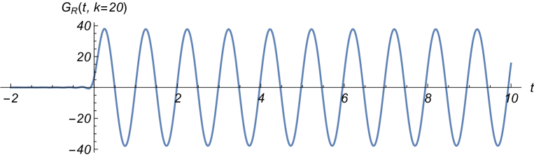
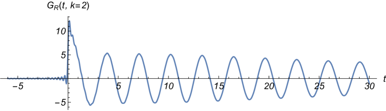
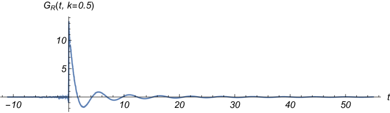
Figure 1: The time-dependence of the surface-to-surface retarded Green’s function $\tilde{G}_{R}(t,\vec{k})$ for gravity waves in an infinitely deep compressional ocean, from large horizontal wavenumbers (top) to small ones (bottom). At wavenumbers smaller than one (in the units discussed in the text), there are no waves propagating at the surface.

As for the cuts, they are located at

$$\omega^{2}=1+\mu^{2}+k^{2}\;,\qquad\mu^{2}\in\mathbb{R}^{+}\;,$$ (117)

where $\mu^{2}$ can be thought of as a coordinate along the cuts. For fixed $\mu^{2}$, this equation is simply the dispersion relation for a relativistic massive particle, with squared mass $M^{2}=1+\mu^{2}>0$. In such a case, as proved in Appendix D, for all complex $k$’s one has

$$|{\rm Im}\,\omega|\leq|{\rm Im}\,k|\;,$$ (118)

with the equality being attained only for ${\rm Im}\,k=0$. Moreover, splitting $\omega$ and $k^{2}$ into their real and imaginary parts, the imaginary part of (117) yields

$${\rm Re}(\omega){\rm Im}(\omega)={\textstyle\frac{1}{2}}\,{\rm Im}(k^{2})\;.$$ (119)

This equation tells us that the cuts lie along hyperbolae in the complex $\omega$ plane, identified by the imaginary part of $k^{2}$. After originating at the branch points ($\mu^{2}=0$), the cuts approach the real axis as

$${\rm Im}\,\omega\propto\frac{1}{{\rm Re}\,\omega}\;.$$ (120)

The analytic structure just described is shown in fig. 2.

We thus see that, for fixed but arbitrary complex $k^{2}$, the non-analyticities of (111) extend only up to some finite value of ${\rm Im}(\omega)$, and approach the real axis at ${\rm Re}(\omega)\to\pm\infty$. This allows us to redefine (112) for arbirtrary complex $k^{2}$ as the integral along a continuously deformed contour that avoids all the singularities but coincides with the original one for ${\rm Re}(\omega)\to\pm\infty$, such as that depicted in fig. 2. Such a definition coincides with the original one in (112) for real, positive $k^{2}$, but is however analytic for all complex $k^{2}$, because it is a convergent integral of an analytic function of $k^{2}$, eq. (111).

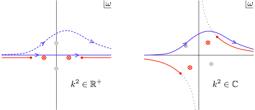
Figure 2: The analytic structure and contours described in the sect. 8.2. The greyed-out poles are in the second sheet, and one need not worry about them. The other poles also move to the second sheet for $|{\rm Re}\,k|<1$.

We thus reach the conclusion that, even though we are not able to compute the integral (112) explicitly, its output can be analytically extended to the whole complex $k^{2}$ plane.

We now come to the question of exponential boundedness. According to our definition of $G_{R}(t,\vec{k}\,)$ for complex $k^{2}$, we have

$$\tilde{G}_{R}(t,\vec{k}\,)=\int_{\gamma}\frac{d\omega}{2\pi}\,\hat{G}_{R}(\omega,\vec{k}\,)e^{-i\,{\rm Re}(\omega)t}e^{{\rm Im}(\omega)t}\;,$$ (121)

where $\gamma$ is the contour avoiding all singularities we just described. Up to non-exponential factors, we thus have

$$|\tilde{G}_{R}(t,k^{2})|\lesssim e^{\max_{\gamma}({\rm Im}\,\omega)\,t}\;,$$ (122)

and $\gamma$ can be pushed as low as the branch cuts and the poles on the first sheet.

As noted above, on the cuts we have $|{\rm Im}\,\omega|\leq|{\rm Im}\,k|$. The poles on the first sheet obey

$$\omega_{\rm pole}^{2}=2k$$ (123)

Taking the imaginary part, we have

$${\rm Re}(\omega_{\rm pole}){\rm Im}(\omega_{\rm pole})={\rm Im}\,k\;.$$ (124)

However, recall that these poles are on the first sheet only for $|{\rm Re}(k)|\geq 1$, which, using (123), implies

$${\rm Re}(\omega_{\rm pole})^{2}\geq{\rm Im}(\omega_{\rm pole})^{2}+2\geq 2\;.$$ (125)

Putting these two equations together we find

$$|{\rm Im}\,\omega_{\rm pole}|\leq\frac{|{\rm Im}\,k|}{\sqrt{2}}<|{\rm Im}\,k|\;.$$ (126)

In conclusion, our retarded Green’s function is analytic in $\vec{k}$ and bounded by

$$|\tilde{G}_{R}(t,\vec{k})|\lesssim e^{|{\rm Im}\,k|\,t}\;,$$ (127)

and thus obeys sonic microcausality, as expected.

9 Microcausality in cosmology

We now switch to curved spacetime and study if and how microcausality can be used to derive bounds on effective field theories in cosmological backgrounds. In this section, for convenience, we adopt the mostly plus signature.

9.1 Scalar field in de Sitter space

We start by analyzing a massless scalar field in de Sitter space. We want to check how its two-point function satisfies the analyticity and boundedness implied by microcausality through the Paley-Wiener theorem. We adopt flat slicing coordinates for de Sitter

$$ds^{2}=\dfrac{1}{H^{2}\tau^{2}}\Big{(}-d\tau^{2}+d\vec{x}\,^{2}\Big{)},$$ (128)

where $H$ is constant and $-\infty<\tau<0$. This is the de Sitter version of Poincaré coordinates. In particular, the lightcone corresponds to $|\Delta\vec{x}|=|\Delta\tau|$. Consider now a massless scalar in de Sitter,

$$S_{\rm free,dS}=\int\sqrt{-g}\left(-\dfrac{1}{2}g^{\mu\nu}\partial_{\mu}\phi\partial_{\nu}\phi\right)d^{4}x=\frac{1}{2}\int\dfrac{1}{H^{2}\tau^{2}}\left((\partial_{\tau}\phi)^{2}-(\partial_{i}\phi)^{2}\right)d\tau d^{3}x\,.$$ (129)

Choosing the Bunch-Davies vacuum by requiring that the two point function of $\phi$ reduces to the flat space result at early times with the correct normalization, we obtain the mode functions

$$f_{k}(\tau)=\dfrac{H}{\sqrt{2k^{3}}}\left(1+ik\tau\right)e^{-ik\tau},$$ (130)

where we used the notation of appendix A. To check microcausality we need to check analyticity and boundedness of

$$\tilde{G}_{c}(\tau_{1},\tau_{2},k) =2i\,{\rm Im}\left(f_{k}(\tau_{1})f_{k}^{*}(\tau_{2})\right)$$ (131)

$$=i\,\dfrac{H^{2}}{k^{3}}\Big{(}k(\tau_{1}-\tau_{2})\cos\big{(}k(\tau_{1}-\tau_{2})\big{)}-(1+k^{2}\tau_{1}\tau_{2})\sin\big{(}k(\tau_{1}-\tau_{2})\big{)}\Big{)}\;.$$

It is straightforward to check that this is analytic in complex $k^{2}$. Moreover, in the complex $k$ plane it is exponentially bounded by

$$|\tilde{G}_{c}(\tau_{1},\tau_{2},k)|\lesssim e^{|{\rm Im}\,k|\,|\tau_{1}-\tau_{2}|}\;.$$ (132)

This result is consistent with microcausality in the fixed de Sitter background (128), whose lightcone is determined by the condition $-d\tau^{2}+d\vec{x}\,^{2}=0$. For fixed $\tau_{1},\tau_{2}$, microcausality implies the vanishing of the position space commutator for $(\vec{x}_{1}-\vec{x}_{2})^{2}>(\tau_{1}-\tau_{2})^{2}$, which is equivalent to (132) through the Paley-Wiener theorem.

9.2 The EFT of inflation

We now consider the case in which the universe undergoes a phase of near-exponential inflation driven by a scalar field $\phi$. The scalar evolves according to a homogeneous time-dependent background solution $\phi_{0}(t)$, while the metric is a flat FRW background

$$ds^{2}=-dt^{2}+a(t)^{2}d\vec{x}\,^{2},$$ (133)

with $H(t)\equiv\dot{a}/a$. It is also useful to define the slow-roll parameters

$$\epsilon\equiv-\dfrac{\dot{H}}{H^{2}},\qquad\eta\equiv\dfrac{\dot{\epsilon}}{H\epsilon}.$$ (134)

The dynamics of the scalar field and of gravity are now mixed and we cannot treat $\phi$ as a simple test field on a fixed background. We use comoving (unitary) gauge in which the perturbations are defined by the conditions

$$\phi(t,\vec{x})=\phi_{0}(t),\qquad h_{ij}=a^{2}(t)\left(e^{2\zeta(t,\vec{x})}\delta_{ij}+\gamma_{ij}\right).$$ (135)

$h_{ij}$ is the induced metric on spatial slices defined by $\phi=\rm const$, $\zeta$ denotes the curvature perturbation in comoving gauge, sometimes called $\mathcal{R}$, and $\gamma_{ij}$ is transverse and traceless and parametrizes tensor modes.

The effective action for perturbations can be derived in great generality, without specifying the detailed dynamics of the underlying UV model, using the effective field theory of inflation Cheung:2007st .

At quadratic order, for curvature perturbations one gets

$$S_{\zeta}=\frac{1}{2}\int dtd^{3}x\,\frac{2M_{\rm Pl}^{2}\epsilon}{c_{s}^{2}}a^{3}\Big{(}\dot{\zeta}^{2}-c_{s}^{2}\frac{(\partial_{i}\zeta)^{2}}{a^{2}}\Big{)},$$ (136)

where $M_{\rm Pl}^{2}\equiv 1/(8\pi G)$ and the sound speed $c_{s}$ is defined by

$$\dfrac{1}{c_{s}^{2}}=1-\dfrac{2M_{2}^{4}}{M_{\rm Pl}^{2}\dot{H}}\;,$$ (137)

where $M_{2}(t)^{4}$ is the coefficient of the operator $(\delta g^{00})^{2}/2$ in the EFT of inflation. For instance, for a theory with action $S=\int\sqrt{-g}\,P(X,\phi)$, it is given by

$$M_{2}(t)^{4}=\dot{\phi}^{4}_{0}(t)\dfrac{\partial^{2}P(X,\phi)}{\partial X^{2}}\Bigg{|}_{\phi_{0}},\qquad{\rm where}\qquad X=g^{\mu\nu}\partial_{\mu}\phi\partial_{\nu}\phi.$$ (138)

Higher derivative corrections give Hubble-suppressed terms, which are negligible as long as $H$ is much smaller than the scales $M_{n}$ appearing in the EFT. For a $P(X,\phi)$ theory this corresponds to requirement that the UV scale $\Lambda$ suppressing higher powers of $X$ be parametrically smaller than $M_{\rm Pl}$, with $\Lambda^{2}/M_{\rm Pl}^{2}\ll\epsilon$.

It is convenient to adopt a new time variable $T$, which is related to conformal time but takes into account a possible time-dependence of $c_{s}$,

$$dT\equiv\frac{c_{s}(t)}{a(t)}dt\;.$$ (139)

The quadratic action simply becomes

$$S_{\zeta}=\frac{1}{2}\int dTd^{3}x\,Z(T)\Big{(}\zeta^{\prime}\,{}^{2}-(\partial_{i}\zeta)^{2}\Big{)}\;,\qquad Z(T)\equiv\frac{2M_{\rm Pl}^{2}\epsilon(T)}{c_{s}(T)}a^{2}(T)\;,$$ (140)

where primes denote derivatives w.r.t. $T$. The equation of motion for the mode functions takes the form

$$\zeta_{k}^{\prime\prime}+\dfrac{Z^{\prime}}{Z}\,\zeta_{k}^{\prime}+k^{2}\,\zeta_{k}=0\;,$$ (141)

where the “Hubble friction” coefficient is

$$\dfrac{Z^{\prime}}{Z}=\frac{aH}{c_{s}}\left(2+{\eta-s}\right),\qquad{\rm with}\quad s\equiv\dfrac{\dot{c}_{s}}{Hc_{s}}\;.$$ (142)

Up to now we did not make any slow-roll approximation. In order to find explicit solutions to this equations and derive constraints from microcausality we will now assume the slow-roll conditions that $\epsilon,\eta,s$ are much smaller than one, and solve our equation by keeping first-order terms only,

$$\zeta_{k}^{\prime\prime}+\dfrac{1-2\nu}{T}\,\zeta_{k}^{\prime}+k^{2}\,\zeta_{k}=0,\qquad{\rm where}\quad\nu\equiv\dfrac{1}{2}\big{(}3+2\epsilon+{\eta+s}\big{)}\;,$$ (143)

where since the only explicitly time-dependent parameters are of first-order in the slow-roll expansion, we can consistently treat $\nu$ as constant.

The above equation can be solved in terms of Hankel functions,

$$\zeta_{k}(\tau)=c_{1}\cdot(-T)^{\nu}H^{(1)}_{\nu}(-kT)+c_{2}\cdot{(-T)^{\nu}}H^{(2)}_{\nu}(-kT)\;.$$ (144)

The solution that has positive frequency at early times,

$$\zeta_{k}(T)\propto e^{-ik\,T},\qquad T\to-\infty$$ (145)

can be singled out by considering the asymptotic expansion of the Hankel functions for $T\to-\infty$,

$$H^{(1,2)}_{\nu}(-kT)\simeq\sqrt{\dfrac{2}{\pi(-kT)}}e^{\mp i(kT+\frac{\nu\pi}{2}+\frac{\pi}{4})}\;,$$ (146)

which tells us that $c_{2}$ should vanish. The coefficient $c_{1}$ can be determined from the Klein-Gordon product normalization condition (see eq. (171) in the appendix). Keeping into account the additional non-canonical $Z$ factor in the action (140), after some simple algebra we find

$$\zeta_{k}(\tau) \simeq\dfrac{\sqrt{\pi}}{2M_{\rm Pl}}\sqrt{\frac{-T}{Z(T)}}H^{(1)}_{\nu}(-kT)$$ (147)

$$\simeq\dfrac{\sqrt{\pi}}{2M_{\rm Pl}}\sqrt{\frac{(-T_{\star})^{-2\epsilon-\eta-s}}{\epsilon_{\star}{c_{s}}_{\star}}}H_{\star}\cdot(-T)^{\nu}H^{(1)}_{\nu}(-kT)\;,$$ (148)

where we chose an overall phase, $T_{\star}$ is an arbitrary time, and all starred quantities are evaluated there.

We consider now the constraints from microcausality. From eq. (174), the $\langle[\zeta,\zeta]\rangle$ commutator is

$$\tilde{G}_{c}(T_{1},T_{2};k)=2i\,{\rm Im}\left(\zeta_{k}(T_{1})\zeta_{k}^{*}(T_{2})\right)\propto{\rm Im}\left(H^{(1)}_{\nu}(-kT_{1})H^{(1)}_{\nu}(-kT_{2})^{*}\right)\;,$$ (149)

and this has to be an analytic function of $k^{2}$ and exponentially bounded. Let us first consider analyticity. It is convenient to express $H^{(1)}_{\nu}$ in terms of Bessel-$J$ functions:

$$H^{(1)}_{\nu}(y)=\dfrac{J_{-\nu}(y)-J_{\nu}(y)e^{-i\nu\pi}}{i\sin(\nu\pi)},\qquad H^{(1)}_{\nu}(y){}^{*}=\dfrac{J_{-\nu}(y)-J_{\nu}(y)e^{i\nu\pi}}{-i\sin(\nu\pi)},$$ (150)

where we kept the argument $y$ real in taking the complex conjugate. Then, up to irrelevant factors, our commutator is

$$\tilde{G}_{c}(T_{1},T_{2};k)\propto\Big{(}J_{-\nu}(-kT_{2})J_{\nu}(-kT_{1})-J_{-\nu}(-kT_{1})J_{\nu}(-kT_{2})\Big{)}$$ (151)

It so happens that the Bessel-$J$ functions can be written as

$$J_{\nu}(y)=y^{\nu}f_{\nu}(y^{2})\;,$$ (152)

where $f_{\nu}$ is an entire function of complex $y^{2}$. We thus see that in the commutator above, for arbitrary $T_{1}$ and $T_{2}$, all non-integer powers of $k$ cancel, and we are left with an entire function of $k^{2}$, as required by microcausality.

To check exponential boundedness without having to control non-exponential factors, we can consider the case in which at least one of the two operators is inserted at a large negative time, $kT_{1}\to-\infty$ (with fixed $k$). We stress that in doing so we are not restricting ourselves to probing the dynamics only on subhorizon scales or, equivalently, to considering the local dynamics of small wavepackets in a weakly curved background. In fact, by studying the $kT_{1}\to-\infty$, $kT_{2}\to 0$ case we are following a mode that gets stretched from subhorizon to superhorizon scales in the curved background. Using the asymptotic expansions of $H^{(1)}_{\nu}(y)$,

$$H^{(1)}_{\nu}(y)\simeq\sqrt{\dfrac{2}{\pi y}}e^{i(y-\frac{\nu\pi}{2}-\frac{\pi}{4})},\qquad{\rm for}\qquad y\to\infty$$ (153)

$$H^{(1)}_{\nu}(y)\simeq-\dfrac{i\,\Gamma(\nu)}{\pi}\left(\dfrac{y}{2}\right)^{-\nu},\qquad{\rm for}\qquad y\to 0$$ (154)

for $kT_{1}\to-\infty$, $kT_{2}\to 0$ we get that the commutator is of order

$$\tilde{G}_{c}(T_{1},T_{2};k)\sim\cos\left(-kT_{1}-\frac{\nu\pi}{2}-\frac{\pi}{4}\right)\;,$$ (155)

where we are omitting power-law prefactors. For complex $k$ we thus have

$$|\tilde{G}_{c}(T_{1},T_{2};k)|\sim e^{|{\rm Im}k|\,|T_{1}|}=e^{|{\rm Im}k|\cdot|\int^{\tau_{1}}c_{s}(\tau)d\tau|}\;$$ (156)

where $\tau$ is conformal time: similarly to the de Sitter case, the lightcone of an FRW metric in comoving coordinates is determined by the condition $-d\tau^{2}+d\vec{x}\,^{2}=0$, so that microcausality implies the vanishing of the position space commutator for $(\vec{x}_{1}-\vec{x}_{2})^{2}>(\tau_{1}-\tau_{2})^{2}$. We thus expect exponential boundedness for $\tilde{G}_{c}$ in the form

$$|\tilde{G}_{c}(T_{1},T_{2};k)|\lesssim e^{|{\rm Im}k|\cdot|\tau_{1}-\tau_{2}|}\;,$$ (157)

which in our case is obeyed as long as $c_{s}(\tau)\leq 1$, not surprisingly.

We can repeat the same analysis for the case in which both operators are inserted at early times, $kT_{1,2}\to-\infty$. We find

$$|\tilde{G}_{c}(T_{1},T_{2};k)|\lesssim e^{|{\rm Im}k|\cdot|\int^{\tau_{2}}_{\tau_{1}}c_{s}(\tau)d\tau|},$$ (158)

which again obeys microcausality as long as $c_{s}(\tau)\leq 1$.

From eq. (137), we thus see that in a theory that satisfies the Null Energy Condition (which requires $\dot{H}\leq 0$), microcausality implies

$$M_{2}(t)^{4}\geq 0\quad{\rm in\,the\,EFT\,of\,Inflation,}$$ (159)

$$\dfrac{\partial^{2}P(X,\phi)}{\partial X^{2}}\Bigg{|}_{\phi_{0}(t)}\geq 0\quad{\rm in\;a}\;P(X,\phi)\;{\rm theory}.$$ (160)

This bound is analogous to the similar statement derived in flat space. Notice however that in flat space one can argue that, in an interacting theory, the coefficient has to be strictly positive, whereas our argument only allows us to conclude that it must be non-negative. Moreover, the positivity statement relies on the fact that $\dot{H}\neq 0$ and does not directly apply to de Sitter space.

9.3 The EFT for inflation

We can consider analogous bounds in the so-called effective field theory for inflation Weinberg:2008hq , which corresponds to a different power-counting than that in the effective field theory of inflation Cheung:2007st . Up to field redefinitions and total derivatives the effective action for the inflaton field and gravity up to four derivatives takes the form Weinberg:2008hq

$$S_{\rm EH}=\int d^{4}x\sqrt{-g}\left(\dfrac{M_{\rm Pl}^{2}}{2}R-\dfrac{X}{2}-V(\phi)+f_{1}(\phi)\dfrac{X^{2}}{\Lambda^{4}}+f_{9}(\phi)W^{\mu\nu\rho\sigma}W_{\mu\nu\rho\sigma}\right),$$ (161)

where $X=g^{\mu\nu}\partial_{\mu}\phi\partial_{\nu}\phi$, $W^{\mu\nu\rho\sigma}$ is the Weyl tensor, and we dropped a parity odd $W\tilde{W}$ term that does not contribute to the quadratic action for scalar perturbations. The $f_{1}$ term contributes a correction to the sound speed of scalar perturbations in agreement with eqs. (137) and (138), where

$$\dfrac{\partial^{2}P(X,\phi)}{\partial X^{2}}\Bigg{|}_{\phi_{0}}=\dfrac{2f_{1}(\phi)}{\Lambda^{4}}.$$ (162)

The $f_{9}$ term contributes a correction equivalent to $\Delta f_{1}(\phi)=f_{9}(\phi)\cdot(\Lambda^{4}/3M_{\rm Pl}^{4})$ Weinberg:2008hq . We are left with

$$\dfrac{1}{c_{s}^{2}}=1-\dfrac{4\dot{\phi}_{0}(t)^{4}}{M_{\rm Pl}^{2}\dot{H}}\left(\dfrac{f_{1}(\phi)}{\Lambda^{4}}+\dfrac{f_{9}(\phi)}{3M_{\rm Pl}^{4}}\right).$$ (163)

The analysis of our previous section would then tell us that microcausality implies the positivity bound

$$\left(\dfrac{f_{1}(\phi)}{\Lambda^{4}}+\dfrac{f_{9}(\phi)}{3M_{\rm Pl}^{4}}\right)\geq 0.$$ (164)

While this conclusion is robust in the case in which the UV cutoff that controls the inflaton’s self-interactions is $\Lambda\ll M_{\rm Pl}$, a note of caution is warranted. In deriving bounds from microcausality we assumed a fixed gravitational background and used its light-cone to define microcausality. While this requirement seems reasonable in a framework in which gravity is treated as a classical background Dubovsky:2007ac , the notion of a lightcone become less well defined when dynamical gravity and field redefinitions for the metric are taken into account Adams:2006sv ; Bordin:2017hal . One possibility would be to define an underlying Minkowski space and treat the metric just as a tensor field living in such a flat space Visser:1998ua ; Adams:2006sv , but this procedure appears to be plagued by gauge ambiguities Gao:2000ga . So, our best hope to take advantage of microcausality in curved space seems to be that of sticking with a fixed background. The effects of dynamical gravity, together with quantum gravitational corrections, pollute the sharpness of the lightcone with $M_{\rm Pl}$ suppressed corrections, so that our statements are informative only when $M_{\rm Pl}$ suppressed effects can be neglected. This state of affairs closely parallels the case of S-matrix positivity bounds, where in the presence of dynamical gravity a $t$-channel pole in the forward limit complicates the analysis of gravitational theories, and in fact allows small regions of negativity Caron-Huot:2021rmr .

10 Discussion

We appear to live in a universe where Lorentz symmetry, if it’s broken at all, is broken spontaneously. Microcausality is thus expected to be satisfied, regardless of what Lorentz-breaking state one happens to be considering. As such, the commutator Green’s function $G_{c}$ (3), expressed as a function of time $t$ in (spatial) Fourier space, should (1) be analytic in the complex vector $\vec{k}$, and (2) be exponentially bounded, according to the Paley-Wiener theorem (7). These two statements combined can be shown to be equivalent to the vanishing of $G_{c}$ outside the lightcone in real space. When rotation is not broken, the analyticity property translates into analyticity in the complex $k^{2}\equiv\vec{k}\cdot\vec{k}$. And when considering an EFT, taking the large $kt$ limit while staying within the regime of validity of the EFT, it’s sufficient to focus on the exponential in exponential boundedness (21).

We consider the implications of these statements in a variety of settings, from superfluids, solids/framids, normal fluids to inflation. A few recurring themes emerge from these examples: (1) Not surprisingly, microcausality typically implies subluminal sound speed, though see Sec. 5.2 on the possibility of superluminal group velocity. (2) In verifying microcausality in an EFT, it’s crucial that one stays within the regime of validity of the EFT, i.e. $k$ and $\omega$ must stay below the cut-off of the theory in question. (3) In systems where multiple gapless degrees of freedom are present, analyticity sometimes requires cancelation among their respective contributions to the Green’s function. An example is the solid/framid with its longitudinal and transverse modes (Sec. 7). (4) In verifying the analyticity of the Green’s function in $(t,\vec{k})$ space, one might encounter an integral over $\omega$ for which care must be taken in choosing the integration contour. An example on gravity waves is discussed in Sec. 8.2. (5) Microcausality as stated so far concerns the two-point function, but in some cases, can be used to make statement about interactions. Examples can be found in the discussions on superfluid (Sec. 5.1) and on inflation (Sec. 9.3), where one starts from a manifestly Lorentz invariant theory and proceeds to consider a Lorentz violating background.

The last point raises a natural question: can we formulate a statement of microcausality that can be applied directly to higher-point functions? Consider the following nested commutator:

$$[{\cal O}_{3}(t,\vec{x}_{3}),[{\cal O}_{2}(t,\vec{x}_{2}),{\cal O}_{1}(0,0)]]\,.$$ (165)

It’s obvious that this vanishes if $(t,\vec{x}_{2})$ and $(0,0)$ are space-like separated. Making use of the Jacobi identity, and the fact that ${\cal O}_{3}$ and ${\cal O}_{2}$ are at equal time and therefore commute, we see that this nested commutator also vanishes if $(t,\vec{x}_{3})$ and $(0,0)$ are space-like separated. Thus, the corresponding 3-point function:

$$G_{c}^{(3)}(t,\vec{x}_{2},\vec{x}_{3})\equiv\langle[{\cal O}_{3}(t,\vec{x}_{3}),[{\cal O}_{2}(t,\vec{x}_{2}),{\cal O}_{1}(0,0)]]\rangle$$ (166)

vanishes if $|\vec{x}_{2}|^{2}>t^{2}$ or $|\vec{x}_{3}|^{2}>t^{2}$. Fourier transforming into $G_{c}^{(3)}(t,\vec{k}_{2},\vec{k}_{3})$ and invoking the Paley-Weiner theorem, we conclude $G_{c}^{(3)}(t,\vec{k}_{2},\vec{k}_{3})$ is analytic in complex $\vec{k}_{2}$ and $\vec{k}_{3}$, and is bounded by $e^{({||{\rm Im\,}\vec{k}_{3}\,||}+{||{\rm Im\,}\vec{k}_{2}\,||})\cdot|t|}$ up to prefactor. This statement can be straightforwardly generalized to

$$G_{c}^{(n)}(t,\vec{x}_{2},...\vec{x}_{n-1},\vec{x}_{n})\equiv\langle[{\cal O}_{n}(t,\vec{x}_{n}),[{\cal O}_{n-1}(t,\vec{x}_{n-1}),....[{\cal O}_{2}(t,\vec{x}_{2}),{\cal O}_{1}(0,0)]...]]\rangle\,,$$ (167)

which vanishes if any of the $|\vec{x}_{2}|^{2},...,|\vec{x}_{n}|^{2}$ exceeds $t^{2}$, resulting in analogous analyticity and boundedness statements on $G_{c}^{(n)}(t,\vec{k}_{2},...,\vec{k}_{n})$. It would be interesting to use these higher-point Green’s functions to constrain interacting theories with broken Lorentz, such as those that occur naturally in cosmology. We hope to explore this in the near future.

Appendix

Appendix A Some useful expressions for commutator two-point functions

We collect here some results on commutators of scalar fields in homogeneous and isotropic backgrounds. This assumption is not essential but simplifies some of the computations, while being general enough to treat interesting cases such as cosmological backgrounds, including inflation, superfluids, fluids, and relativistic hydrodynamics.

Free scalars.

Consider a (real) free scalar field $\phi(t,\vec{x})$ and assume that in canonical quantization it is quantized in terms of classical mode functions $u_{\bf k}$ of the form

$$u_{\bf k}(t,\vec{x})=f_{k}(t)e^{i\vec{k}\cdot\vec{x}},\qquad u^{*}_{\bf k}(t,\vec{x})=f^{*}_{k}(t)e^{-i\vec{k}\cdot\vec{x}}.$$ (168)

The field operator $\hat{\phi}$ and its conjugate momentum $\hat{\Pi}$ are then given by

$$\hat{\phi}(t,\vec{x})=\int\dfrac{d^{3}k}{(2\pi)^{3}}\left(u_{\bf k}(t,\vec{x})\hat{a}_{\bf k}+u^{*}_{\bf k}(t,\vec{x})\hat{a}^{\dagger}_{\bf k}\right),\qquad\hat{\Pi}(t,\vec{x})=\sqrt{h}\,\partial_{t}\phi\,,$$ (169)

where we denote by $h$ the spatial metric. The mode functions are normalized so that

$$\langle u_{\bf k},u_{\bf k^{\prime}}\rangle=(2\pi)^{3}\delta^{(3)}({\bf k}-{\bf k^{\prime}}),\qquad\langle u^{*}_{\bf k},u^{*}_{\bf k^{\prime}}\rangle=-(2\pi)^{3}\delta^{(3)}({\bf k}-{\bf k^{\prime}}),\qquad\langle u_{\bf k},u^{*}_{\bf k^{\prime}}\rangle=0,$$ (170)

with respect to the Klein-Gordon inner product, see for instance Birrell:1982ix . The normalization condition on the mode functions (168) can be expressed as

$$i\sqrt{h}\sqrt{g^{00}}(f_{k}^{*}\partial_{t}f_{k}-\partial_{t}f_{k}^{*}f_{k})=1.$$ (171)

With this normalization the equal-time canonical commutation relations

$$[\hat{\phi}(t,{\bf x}),\hat{\Pi}(t,{\bf x^{\prime}})]=i\delta^{(3)}({\bf x}-{\bf x^{\prime}})$$ (172)

are recovered for $[\hat{a}_{\bf k},\hat{a}^{\dagger}_{\bf k^{\prime}}]=(2\pi)^{3}\delta^{(3)}({\bf k}-{\bf k^{\prime}})$, and $[\hat{a}_{\bf k},\hat{a}_{\bf k^{\prime}}]=0$.

The commutator between two fields inserted at different spacetime points can now be easily computed and is given by

$$[\hat{\phi}(t_{1},\vec{x}_{1}),\hat{\phi}(t_{2},\vec{x}_{2})]=\int\dfrac{d^{3}k}{(2\pi)^{2}}\,2i\,{\rm Im}\left(f_{k}(t_{1})f_{k}^{*}(t_{2})\right)e^{i\vec{k}\cdot(\vec{x}_{1}-\vec{x}_{2})}.$$ (173)

Thanks to translational and rotational invariance, this is a function of $(\vec{x}_{1}-\vec{x}_{2})^{2}$ only and its Fourier transform with respect to spatial coordinates depends on the spatial momentum only through $k^{2}$. This expressions is valid as an operator statement, where on the right the identity operator is understood. It can be evaluated in arbitrary states or inserted in a generic multipoint correlation functions. When evaluated on the ground state it corresponds to the commutator Green’s function: we will only focus on this correlator and leave an analysis of more general correlation functions to future work.

It is the useful to define the Fourier transform with respect to $(\vec{x}_{1}-\vec{x}_{2})$:

$$\tilde{G}_{c}(t_{1},t_{2},\vec{k})\equiv 2i\,{\rm Im}\left(f_{k}(t_{1})f_{k}^{*}(t_{2})\right).$$ (174)

Since the commutator vanishes for space-like separations, $\tilde{G}_{c}(t_{1},t_{2},k)$ is constrained by the Paley-Wiener theorem to be analytic in $k^{2}$ and exponentially bounded as reviewed in section 2. We stress that this property is a necessary and sufficient condition for microcausality.

Commutator in terms of $T$-ordered two-point function.

When including interactions it is often convenient to study time-ordered correlators, and take advantage of Feynman rules and perturbative tools to compute loop correction. It is therefore useful to write the commutator Green’s function in terms of the time-ordered two-point function. It is convenient to do this either in frequency or in position space. We find

$$\hat{G}_{c}(\omega,\vec{k})=2\,{\rm sign}(\omega)\,{\rm Re}\,\hat{G}_{T}(\omega,\vec{k})$$ (175)

$$G_{c}(t,\vec{x})=2i\,{\rm sign}(t)\,{\rm Im}\,{G}_{T}(t,\vec{x})$$ (176)

These relations are fully non-perturbative. The former follows from a spectral representation of two-point functions—see e.g. Weinberg:1995mt . The latter follows immediately from the definitions of commutators and time-order correlators.

Appendix B Complex $\vec{k}$ vs. complex $k$

For any complex vector $\vec{k}\in\mathbb{C}^{3}$, define its real and imaginary parts

$$\vec{k}=\vec{R}+i\vec{I}\;,\qquad\vec{R},\vec{I}\in\mathbb{R}^{3}\;.$$ (177)

Then,

$$k^{2}\equiv\vec{k}\cdot\vec{k}=R^{2}-I^{2}+2i\,RI\cos\theta\;,$$ (178)

where $R\geq 0$ and $I\geq 0$ are the magnitudes of the corresponding real vectors, and $\theta$ is the angle between such vectors.

On the other hand, defining the complex number

$$k\equiv\sqrt{k^{2}}$$ (179)

and splitting it into its real and imaginary parts,

$$k={\cal R}+i{\cal I}\;,\qquad{\cal R},{\cal I}\in\mathbb{R}\;,$$ (180)

we have

$$k^{2}=k\,k={\cal R}^{2}-{\cal I}^{2}+2i\,{\cal R}{\cal I}\;.$$ (181)

Equating the two expression for $k^{2}$ and squaring the imaginary parts we get

$$R^{2}-I^{2} ={\cal R}^{2}-{\cal I}^{2}$$ (182)

$$R^{2}I^{2}\cos^{2}\theta ={\cal R}^{2}{\cal I}^{2}\;.$$ (183)

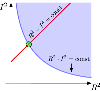
Figure 3: The geometry of certain real and imaginary parts described in the text.

Now, if we have an analytic function of $k^{2}$ bounded by

$$e^{||{\rm Im}\,\vec{k}\,||\cdot|t|}=e^{I\,|t|}\;,$$ (184)

it must be in fact bounded by the minimum of such an exponential over all possible complex vectors $\vec{k}$ that have the same $k^{2}$, or, equivalently, the same $k={\cal R}+i{\cal I}$. Plotting the conditions (182), (183) in the $(R^{2},I^{2})$ place for fixed ${\cal R}$ and ${\cal I}$—see fig. 3—, and keeping into account that $\cos^{2}\theta<1$, it is clear that the minimum of $I$ for constant $k$ is achieved for $R^{2}={\cal R}^{2}$, $I={\cal I}^{2}$, $\cos^{2}\theta=1$.

Therefore, our analytic function of $k^{2}$ should in fact be bounded by

$$e^{|{\cal I}|\,|t|}=e^{|{\rm Im}\,k|\,|t|}\;.$$ (185)

Appendix C Analyticity in $(\omega,\vec{k}\,)$ space

In the case of correlation functions in the mixed $(t,\vec{k}\,)$ representation, the analyticity and boundedness criterion is obtained for fixed $t$ or, in the distributional case, after smearing on time-dependent test functions of compact support. After Fourier transforming to frequency space, the analyticity statement one should check becomes: $\hat{G}_{c}(\omega,\vec{k})$ is a $\vec{k}$-dependent distribution in $\omega$ such that, when applied to any analytic test function $f(\omega)$, yields an analytic function of $\vec{k}$. This is because compact support functions are mapped to analytic functions under Fourier transform.

Let us look at the example of a free scalar in a Lorentz invariant theory. The commutator two-point function in frequency space is

$$\hat{G}_{c}(\omega,\vec{k})=2\pi\,{\rm sign}(\omega)\,\delta(p^{2}-M^{2}).$$ (186)

If we consider this as a distribution in $\omega$ on the space of analytic test functions $f(\omega)$, after integrating we obtain

$$\int\hat{G}_{c}(\omega,\vec{k})\,f(\omega)\dfrac{d\omega}{2\pi}=\dfrac{f(\omega_{k})}{2\omega_{k}}-\dfrac{f(-\omega_{k})}{2\omega_{k}}=\dfrac{f(\omega_{k})-f(-\omega_{k})}{2\omega_{k}}.$$ (187)

It easy easy to see that this is an even analytic function of $\omega_{k}=\sqrt{k^{2}+M^{2}}$, and thus an analytic function of $\vec{k}$.

The boundedness criterion is obtained after taking into account the exponential boundedness of the analytic test functions to which the compact support time-dependent test function are mapped under Fourier transform.

Appendix D ${\rm Im}\,\omega_{k}$ vs. ${\rm Im}\,k$

We want to show that

$$|{\rm Im}(\omega_{k})|\equiv|{\rm Im}(\sqrt{k^{2}+M^{2}})|\leq|{\rm Im}(k)|\;,\qquad(M^{2}\geq 0,\;k\in\mathbb{C})\;.$$ (188)

This is trivially true for $M=0$, therefore Let us focus on the case $M\neq 0$. Upon rescaling $k$ by $M$, this is the same as

$$|{\rm Im}(\sqrt{1+k^{2}})|\leq|{\rm Im}(k)|\;.$$ (189)

To prove this, we split $k$ and $\sqrt{1+k^{2}}$ into their real and imaginary parts

$$k={\cal R}+i\,{\cal I}\;,\qquad\sqrt{1+k^{2}}=R+i\,I\;,$$ (190)

and use the identity

$$(\sqrt{1+k^{2}})^{2}=1+(k)^{2}\;,$$ (191)

to obtain the equations

$$R^{2}-I^{2} =1+{\cal R}^{2}-{\cal I}^{2},$$ (192)

$$R^{2}\cdot I^{2} ={\cal R}^{2}\cdot{\cal I}^{2}.$$ (193)

The relevant geometry is still that of fig. 3.

We see that $R^{2}$ and $I^{2}$ are two nonnegative numbers whose product is the same as that of two other nonnegative numbers, ${\cal R}^{2}$ and ${\cal I}^{2}$, but whose difference is larger. We must have

$$R^{2}>{\cal R}^{2}\;,\qquad I^{2}\leq{\cal I}^{2}\;,$$ (194)

with the equality being attained only for $I={\cal I}=0$.

Therefore, in the whole $k$ complex plane, we have

$$|{\rm Re}\,\omega_{k}|>|{\rm Re}\,k|\;,\qquad|{\rm Im}\,\omega_{k}|\leq|{\rm Im}\,k|\qquad\qquad(M^{2}>0)\;.$$ (195)

Notice that the same analysis applies in the case of a tachyon, $M^{2}<0$, and yields the opposite inequalities,

$$|{\rm Re}\,\omega_{k}|<|{\rm Re}\,k|\;,\qquad|{\rm Im}\,\omega_{k}|\geq|{\rm Im}\,k|\qquad\qquad(M^{2}<0)\;.$$ (196)

References

- (1) F. Strocchi, Selected Topics on the General Properties of Quantum Field Theory. World Scientific, 1993, 10.1142/1807.
- (2) S. Dubovsky, A. Nicolis, E. Trincherini and G. Villadoro, Microcausality in curved space-time, Phys. Rev. D 77 (2008) 084016 [0709.1483].
- (3) P. Creminelli, O. Janssen and L. Senatore, Positivity bounds on effective field theories with spontaneously broken Lorentz invariance, JHEP 09 (2022) 201 [2207.14224].
- (4) M. P. Heller, A. Serantes, M. Spaliński and B. Withers, Rigorous Bounds on Transport from Causality, Phys. Rev. Lett. 130 (2023) 261601 [2212.07434].
- (5) P. Creminelli, O. Janssen, B. Salehian and L. Senatore, Positivity bounds on electromagnetic properties of media, JHEP 08 (2024) 066 [2405.09614].
- (6) E. M. Stein and R. Shakarchi, Complex Analysis, Princeton Lectures in Analysis. Princeton University Press, 2003.
- (7) N. N. Bogolubov, A. A. Logunov, A. I. Oksak and I. T. Todorov, eds., General Principles of Quantum Field Theory, vol. 10 of Mathematical Physics and Applied Mathematics. Springer, 1990, 10.1007/978-94-009-0491-0.
- (8) P. Kravchuk, J. Qiao and S. Rychkov, Distributions in CFT. Part II. Minkowski space, JHEP 08 (2021) 094 [2104.02090].
- (9) T. J. Hollowood and G. M. Shore, Causality and Micro-Causality in Curved Spacetime, Phys. Lett. B 655 (2007) 67 [0707.2302].
- (10) T. J. Hollowood and G. M. Shore, The Refractive index of curved spacetime: The Fate of causality in QED, Nucl. Phys. B 795 (2008) 138 [0707.2303].
- (11) T. J. Hollowood and G. M. Shore, Causality Violation, Gravitational Shockwaves and UV Completion, JHEP 03 (2016) 129 [1512.04952].
- (12) A. V. Manohar, Introduction to Effective Field Theories, 1804.05863.
- (13) A. Adams, N. Arkani-Hamed, S. Dubovsky, A. Nicolis and R. Rattazzi, Causality, analyticity and an IR obstruction to UV completion, JHEP 10 (2006) 014 [hep-th/0602178].
- (14) J. D. Jackson, Classical Electrodynamics. Wiley, 1998.
- (15) E. M. Lifshitz and L. P. Pitaevskii, Statistical physics: theory of the condensed state, vol. 9. Elsevier, 2013.
- (16) L. Hui, I. Kourkoulou, A. Nicolis, A. Podo and S. Zhou, S-matrix positivity without Lorentz invariance: a case study, JHEP 04 (2024) 145 [2312.08440].
- (17) P. Creminelli, M. Delladio, O. Janssen, A. Longo and L. Senatore, Non-analyticity of the S-matrix with spontaneously broken Lorentz invariance, JHEP 06 (2024) 201 [2312.08441].
- (18) A. Esposito, R. Krichevsky and A. Nicolis, Solidity without inhomogeneity: Perfectly homogeneous, weakly coupled, UV-complete solids, JHEP 11 (2020) 021 [2004.11386].
- (19) A. Nicolis, R. Penco, F. Piazza and R. Rattazzi, Zoology of condensed matter: Framids, ordinary stuff, extra-ordinary stuff, JHEP 06 (2015) 155 [1501.03845].
- (20) D. Blas and S. Sibiryakov, Horava gravity versus thermodynamics: The Black hole case, Phys. Rev. D 84 (2011) 124043 [1110.2195].
- (21) P. Creminelli, J. Norena, M. Pena and M. Simonovic, Khronon inflation, JCAP 11 (2012) 032 [1206.1083].
- (22) P. Kovtun, Lectures on hydrodynamic fluctuations in relativistic theories, J. Phys. A 45 (2012) 473001 [1205.5040].
- (23) A. Joyce, A. Nicolis, A. Podo and L. Santoni, Integrating out beyond tree level and relativistic superfluids, JHEP 09 (2022) 066 [2204.03678].
- (24) A. Nicolis, A. Podo and L. Santoni, The connection between nonzero density and spontaneous symmetry breaking for interacting scalars, JHEP 09 (2023) 200 [2305.08896].
- (25) R. Baier, P. Romatschke, D. T. Son, A. O. Starinets and M. A. Stephanov, Relativistic viscous hydrodynamics, conformal invariance, and holography, Journal of High Energy Physics 2008 (2008) 100.
- (26) L. D. Landau and E. M. Lifshitz, Fluid Mechanics: Volume 6, vol. 6. Elsevier, 1987.
- (27) D. Baumann, D. Green and T. Hartman, Dynamical Constraints on RG Flows and Cosmology, JHEP 12 (2019) 134 [1906.10226].
- (28) C. de Rham, A. J. Tolley and J. Zhang, Causality Constraints on Gravitational Effective Field Theories, Phys. Rev. Lett. 128 (2022) 131102 [2112.05054].
- (29) D. Green, Y. Huang, C.-H. Shen and D. Baumann, Positivity from Cosmological Correlators, JHEP 04 (2024) 034 [2310.02490].
- (30) M. Carrillo González, Bounds on EFT’s in an expanding universe, Phys. Rev. D 109 (2024) 085008 [2312.07651].
- (31) Y. Donath and E. Pajer, The in-out formalism for in-in correlators, JHEP 07 (2024) 064 [2402.05999].
- (32) C. Cheung, P. Creminelli, A. L. Fitzpatrick, J. Kaplan and L. Senatore, The Effective Field Theory of Inflation, JHEP 03 (2008) 014 [0709.0293].
- (33) S. Weinberg, Effective Field Theory for Inflation, Phys. Rev. D 77 (2008) 123541 [0804.4291].
- (34) L. Bordin, G. Cabass, P. Creminelli and F. Vernizzi, Simplifying the EFT of Inflation: generalized disformal transformations and redundant couplings, JCAP 09 (2017) 043 [1706.03758].
- (35) M. Visser, B. Bassett and S. Liberati, Superluminal censorship, Nucl. Phys. B Proc. Suppl. 88 (2000) 267 [gr-qc/9810026].
- (36) S. Gao and R. M. Wald, Theorems on gravitational time delay and related issues, Class. Quant. Grav. 17 (2000) 4999 [gr-qc/0007021].
- (37) S. Caron-Huot, D. Mazac, L. Rastelli and D. Simmons-Duffin, Sharp boundaries for the swampland, JHEP 07 (2021) 110 [2102.08951].
- (38) N. D. Birrell and P. C. W. Davies, Quantum Fields in Curved Space, Cambridge Monographs on Mathematical Physics. Cambridge University Press, Cambridge, UK, 1982, 10.1017/CBO9780511622632.
- (39) S. Weinberg, The Quantum theory of fields. Vol. 1: Foundations. Cambridge University Press, 6, 2005, 10.1017/CBO9781139644167.