General theory of slow non-Hermitian evolution

Abstract

Non-Hermitian systems are widespread in both classical and quantum physics. The dynamics of such systems has recently become a focal point of research, showcasing surprising behaviors that include apparent violation of the adiabatic theorem and chiral topological conversion related to encircling exceptional points (EPs). These have both fundamental interest and potential practical applications. Yet the current literature features a number of apparently irreconcilable results. Here we develop a general theory for slow evolution of non-Hermitian systems and resolve these contradictions. We prove an analog of the adiabatic theorem for non-Hermitian systems and generalize it in the presence of uncontrolled environmental fluctuations (noise). The effect of noise turns out to be crucial due to inherent exponential instabilities present in non-Hermitian systems. Disproving common wisdom, the end state of the system is determined by the final Hamiltonian only, and is insensitive to other details of the evolution trajectory in parameter space. Our quantitative theory, leading to transparent physical intuition, is amenable to experimental tests. It provides efficient tools to predict the outcome of the system’s evolution, avoiding the need to follow costly time-evolution simulations. Our approach may be useful for designing devices based on non-Hermitian physics and may stimulate analyses of classical and quantum non-Hermitian-Hamiltonian dynamics, as well as that of quantum Lindbladian and hybrid-Liouvillian systems.

Contents

1. I Background and the summary of results
2. II Non-Hermitian adiabatic theorem (“naïve theory”)
3. III Slow non-Hermitian evolution in the presence of noise (“advanced theory”)
4. IV Implications for non-Hermitian state conversion
   1. IV.1 Which state wins: the most growing vs the end-point fastest growing
   2. IV.2 Non-chiral state conversion upon encircling the exceptional point
   3. IV.3 Chiral state conversion without encircling the exceptional point
5. V Demonstrating the quantitative accuracy of the advanced theory
6. VI Proposals for experimental verification
7. VII Conclusions
8. A Derivation of analytical results
   1. A.1 Iterative adiabatic expansion
      1. A.1.1 Idea and first orders
      2. A.1.2 Solution to an arbitrary order
      3. A.1.3 Convergence and errors
      4. A.1.4 Subtleties
   2. A.2 The effect of fast noise
      1. A.2.1 Derivation
      2. A.2.2 Physical meaning and implications
9. B Discussion of previous explanations of unusual non-Hermitian state conversion and their connection to our advanced theory of Sec. III
   1. B.1 Non-chiral dynamics with EP encircling
   2. B.2 Chiral dynamics without EP encircling
10. C Further demonstration of quantitative accuracy of the advanced theory
    1. C.1 How we produce the state evolution curves with the advanced theory
    2. C.2 Closed evolution: without encircling the exceptional point
    3. C.3 Closed evolution: with encircling the exceptional point

I Background and the summary of results

In recent years, non-Hermitian Hamiltonians have attracted significant attention in the realms of both classical and quantum physics [1, 2, 3, 4, 5, 6]. In classical physics, they naturally appear in the context of lossy systems: friction in mechanical systems, resistive losses in electric circuits, light absoprtion — all these give rise to non-Hermitian Hamiltonians underlying the system dynamics [1, 2, 3]. In quantum systems, they appear when particles or states have a finite lifetime [7, 8, 3, 9, 10, 11, 12, 13, 14] or if one considers measurements with postselected outcomes [3, 15, 16]. Furthermore, quantum systems in contact with Markovian environment can be described by noisy non-Hermitian Hamiltonians [17, 18, 19, 20, 21] or by the Lindblad equation, whose Liouville superoperator can also be written as a non-Hermitian matrix [22, 23, 24, 25, 26, 27, 28, 29, 30, 31, 32, 33, 34, 35].

Non-Hermitian systems give rise to new effects and behaviors that do not appear in their Hermitian counterparts: e.g., non-Hermitian skin effect [36, 37, 38, 39, 4, 5, 6, 40] or topological phase transitions without gap closing [41]. Capturing the phenomenology of non-Hermitian systems sometimes requires adapting new unconventional methods, e.g., using a non-Bloch band theory instead of the conventional — and successful in Hermitian systems — Bloch theory [42]. The unusual properties of non-Hermitian systems may assist in a number of applications such as enhancing sensing sensitivity [43], manipulating quantum systems [13, 44], creating polarization-locked optical devices [45] and multimode switches [46, 47], or improving performance of quantum algorithms [48].

In this context, one effect that has attracted much attention is non-Hermitian state conversion. Under sufficiently slow non-Hermitian evolution, any initial state of the system is converted to one specific eigenstate of the Hamiltonian [49, 50, 51, 52, 53, 54, 55, 56, 57, 58, 59, 60, 26, 61, 62, 63, 64, 65, 66, 67, 12, 45, 68, 31, 69, 46]. Particularly interesting is the case of closed trajectories, as one can compare the effect of following the evolution in one or the opposite direction. The behavior is then classified as either chiral (the coversion result is different for the two directions) or non-chiral (the conversion result is the same). The chirality has been associated with the mutual location of the evolution trajectory in the parameter space and exceptional points (EPs) [49, 50, 51, 53, 54, 55, 58, 26, 63, 64, 65, 66, 12, 45, 69, 31, 70, 71, 72, 73, 74, 75, 76, 77]. However, a number of numerical and experimental examples is known, when this common intuition is challenged by numerical simulations and experimental data [56, 57, 59, 60, 67, 68, 35]. This underlines the fact that analytical understanding of non-Hermitian state conversion [50, 49, 51, 53, 55] is limited and does not provide an explanation for the latter examples.

It is worthwhile mentioning that recent works [78, 79, 35] stressed the importance of non-adiabaticity effects for non-Hermitian state conversion. References [78, 79] have shown that the result of conversion crucially depends on the degree of adiabaticity (evolution slowness) and that the conversion chirality does not qualitatively depend on the proximity of an EP. In particular, notions of instantaneously and trajectory-averaged dominant eigenstates have been introduced. Notably, these works rely on exact solutions for specific evolution examples — rendering the generality of the conclusions unclear.

The present work tackles the problem of slow non-Hermitian evolution from a general perspective. We develop a general theory of such dynamics in the absence (“naïve theory”) and in the presence (“advanced theory”) of uncontrolled fast perturbations (noise). We show that the inclusion of noise is essential, and its presence drastically alters the dynamics of non-Hermitian systems. The crucial role played by noise is a manifestation of inherent exponential instabilities featured by these systems.

While our theoretical analysis captures the general framework of slow non-Hermitian evolution (both in the presence and absence of EPs), we demonstrate its utility through the study of non-Hermitian state conversion. We demonstrate that the chirality of the conversion indeed has no relation to EPs. Instead, the system state is always converted to the “end-point fastest growing” state (the instantaneously dominant eigenstate at the end of the evolution trajectory). Furthermore, the conversion chirality is fully determined by the behavior of the eigenvalues of the Hamiltonian at the end points of the evolution trajectory.

Our results thus disprove the common wisdom, namely, that complete analysis of spectral evolution throughout the trajecotry taken in parameter space is needed in order to find the system’s final state. In fact, here we show that the slow evolution of such a system is determined by its final point in parameter space, and is insensitive to other characteristics of the trajectory.

Our quantitative theory leads to a transparent physical picture. Its predictions are amenable to experimental tests. Our approach provides efficient tools to theoretically study the slow evolution of the system, avoiding the need to follow costly time-evolution simulations. Our results can be straightforwardly generalized to quantum Lindbladian or hybrid-Liouvillian dynamics.

The structure of the paper is as follows. In Sec. II, we present the general theory of noiseless slow non-Hermitian evolution (“non-Hermitian adiabatic theorem”). We discuss how it predicts the common-wisdom expectations for non-Hermitian state conversion. We include noise into consideration in Sec. III and demonstrate how it changes the predictions for non-Hermitian state conversion. In Sec. IV, we exemplify how the predictions of the noiseless theory can fall wrong, while the noise-aware theory always gives the correct prediction for numerical simulations. We further demonstrate the theory’s quantitative accuracy in Sec. V. In Sec. VI, we discuss how to verify our theory experimentally. We conclude with a brief summary and outlook in Sec. VII.

We also provide several appendices. Appendix A describes the derivation of our analytical theory (both in the absence and presence of noise). Appendix B discusses the previous analytical explanations of unconventional conversion behavior [56, 57, 59, 60]: these have never appealed to the presence uncontrolled perturbations, which we show to be essential; we find most of these explanations erroneous, while one [60] is correct and consistent with our explanation, yet limited in applicability. Appendix C gives further numerical evidence for the quantitative accuracy of our theory.

II Non-Hermitian adiabatic theorem (“naïve theory”)

We consider the problem of evolution under a time-dependent non-Hermitian Hamiltonian $H(t)=H_{s}$ with $s=t/T\in[0,1]$, having in mind the limit of slow evolution, $T\rightarrow\infty$. The key object of interest is the evolution operator

$$\mathcal{U}(T,0)=\mathcal{T}\exp\left(-i\int_{0}^{T}dt\,H(t)\right),$$ (1)

where $\mathcal{T}$ stands for time ordering. Of particular interest is the effect of the evolution operator on the instantaneous eigenbasis of $H(t)$. To this end, we define the instantaneous eigenbasis through diagonalizing the Hamiltonian:

$$H(t)\equiv H_{s}=U(t)D(t)U^{-1}(t)\equiv U_{s}D_{s}U_{s}^{-1}.$$ (2)

The matrix $D(t)$ is composed of the Hamiltonian eigenvalues $\lambda_{n}(t)\equiv\lambda_{n,s}$ standing on the diagonal. The matrix $U(t)\equiv U_{s}$ encodes the instantaneous right eigenvectors of the Hamiltonian, $\left|n(t)\right\rangle=\left|n_{s}\right\rangle=U_{s}\left|n\right\rangle$, where $\left|n\right\rangle$ is a column vector $\left(0,\ldots,0,1,0,\ldots 0\right)^{\mathrm{T}}$ with $1$ on the $n$th postition. Note that we have implicitly assumed that such diagonalization is possible; we will further assume that it is unique. That is, we assume that there are no exceptional or degeneracy points on the evolution trajectory (these may be present elsewhere in the space of control parameters).

We develop a systematic expansion in powers of $T^{-1}$ and show that it is possible to represent the evolution operator as

$$\mathcal{U}(T,0)=U(T)\mathcal{E}(T,0)U^{-1}(0),$$ (3)

$$\mathcal{E}(T,0)=\left(\mathbb{I}+W(T)\right)\\ \times\exp\left(-i\int_{0}^{T}dt\,D(t)\right)\left(\mathbb{I}+\tilde{W}(0)\right).$$ (4)

Here $\mathcal{E}(T,0)$ encodes the evolution operator’s action in the instantaneous eigenbasis. The operators $W(t)$ and $\tilde{W}(t)$ are both $O(T^{-1})$ and are related to the eigenbasis evolution operator, $U^{-1}(t)\partial_{t}U(t)\propto T^{-1}$. Finally, we have neglected corrections $O(T^{-1})$ to the Hamiltonian eigenvalues, $D(t)$, inside the exponential — these are unimportant for our purposes. The derivation, detailed expressions for $W(t)$, $\tilde{W}(t)$, and the omitted corrections to $D(t)$, as well as a discussion of a few subtleties, can be found in Appendix A.1.

We call equations (3–4) the adiabatic theorem for non-Hermitian Hamiltonians. One sees that it is consistent with the common wisdom about non-Hermitian state conversion. Instantaneous eigenstates of the Hamiltonian grow/decay under the Hamiltonian’s action, as characterized by $\mathrm{Im}\,\int_{0}^{T}dt\,\lambda_{n}(t)$; the state with the largest value of this integral dominates the evolution by its end — which is why essentially any initial state gets converted to this “most growing” state.

To our knowledge, our result is the first proof of this conversion property of slow non-Hermitian evolution in complete generality, beyond previous proofs for two-level systems [49, 51, 53, 79]. Note also that the conversion is only accurate up to $O(T^{-1})$, as implied by $W(T)$, and not exponentially accurate in $T$. This has been previously pointed out in Ref. [64].

We note in passing the substantial mathematical literature on adiabatic evolution with non-Hermitian Hamiltonians [80, 81, 82], Hermitian Hamiltonians in complex time [83, 84, 85, 86, 87], or Lindbladians [22, 24, 30]. These works focused mostly on the dynamics within the subspace of the states with the largest $\mathrm{Im}\,\lambda_{n}(t)$ [81, 87, 82], as well as on Landau-Zener transition probabilities [83, 80, 84, 85, 86, 22, 24, 30]. This is distinct from our focus here, namely, conversion between eigenstates with different $\mathrm{Im}\,\lambda_{n}(t)$, for which Eqs. (3–4) provide an explicit answer.

III Slow non-Hermitian evolution in the presence of noise (“advanced theory”)

The consideration above assumed perfectly-controlled slow evolution. However, one cannot expect this in reality. In experiments, noise and uncontrolled perturbations will lead to appearance of an additional term in the Hamiltonian $H(t)\rightarrow\bar{H}(t)=H(t)+\varepsilon\delta H(t)$. In numerical simulations of non-Hermitian dynamics, numerical errors may and will occur. These can similarly be modelled by $\delta H(t)$. While both are typically small, we are dealing with a system that has exponential instabilities. Therefore, incorporating the analysis of perturbations is essential.

Our goal is to calculate the evolution operator in the presence of perturbations:

$$\mathcal{\bar{U}}(T,0)=\mathcal{T}\exp\left(-i\int_{0}^{T}dt\,\bar{H}(t)\right).$$ (5)

If the perturbation $\delta H(t)$ is also slow, the analysis of Sec. II can be repeated with the modified Hamiltonian, leading to a small modification of the instantaneous eigenstates and eigenvalues, but no qualitative change. Yet there is no reason to expect slowness from uncontrolled perturbations.

For fast perturbations, we expand $\mathcal{\bar{U}}(T,0)$ in perturbation series:

$$\mathcal{\bar{U}}(T,0)=\mathcal{U}(T,0)\\ -i\varepsilon\int_{0}^{T}dt_{1}\mathcal{U}(T,t_{1})\delta H(t_{1})\mathcal{U}(t_{1},0)\\ +O\left(\varepsilon^{2}\right),$$ (6)

where

$$\mathcal{U}(t_{2},t_{1})=\mathcal{T}\exp\left(-i\int_{t_{1}}^{t_{2}}dt\,H(t)\right)$$ (7)

represents unperturbed (noiseless) slow evolution and can be expressed in the form (3–4) with appropriately replaced time limits.

Note that $\mathcal{U}(T,0)=\mathcal{U}(T,t_{1})\mathcal{U}(t_{1},0)$ for any $t_{1}$, so that the role of $\delta H(t_{1})$ is to disrupt the noiseless adiabatic evolution at all possible intermediate times. Focus on $\delta H(t_{1})\mathcal{U}(t_{1},0)$. By the time $t_{1}$, essentially any initial state becomes aligned with one specific eigenstate $\left|n(t_{1})\right\rangle$ due to the unperturbed evolution $\mathcal{U}(t_{1},0)$. The perturbation at time $t_{1}$ generates amplitude of order $\varepsilon$ in other (generically — all other) instantaneous eigenstates of $H(t_{1})$. This effectively restarts the non-Hermitian state conversion process — with a new initial state and a different evolution trajectory: $H(t\in[t_{1},T])$ instead of $H(t\in[0,T])$. If the preferred state of $\mathcal{U}(T,t_{1})$ for some $t_{1}$ is different from that of $\mathcal{U}(T,0)$, the evolution outcome will change.

Namely, all states will be converted not to the most growing state (with the largest $\mathrm{Im}\int_{0}^{T}dt\,\lambda_{n}(t)$), but to the “end-point fastest growing” one — the one that has the largest $\mathrm{Im}\,\lambda_{n}(t)$ for the times near the end of the evolution (that is, for $t\in[T(1-y),T]$ for some interval length $yT$). One can understand this from the following consideration: all the “restarts” of conversion at $t_{1}\in[T(1-y),T]$ lead to the same the evolution outcome — conversion to the end-point fastest growing state. We illustrate this point with several numerical examples in Sec. IV.

IV Implications for non-Hermitian state conversion

Here we illustrate the predictions of the general theory above with a few examples using a specific $2\times 2$ non-Hermitian Hamiltonian. We discuss example trajectories that highlight the key effects predicted by our theory.

We use the Hamiltonian

$$H=\begin{pmatrix}\delta(t)+ig(t)&-1\\ -1&-\delta(t)-ig(t)\end{pmatrix}.$$ (8)

For each value of real parameters $\delta$ and $g$, it has two eigenvalues, $\lambda_{\pm}=\pm\sqrt{1+\left(\delta+ig\right)^{2}}$, and the corresponding right eigenstates $\left|\psi_{\pm}\right\rangle$. The Hamiltonian possesses two EPs: $\left(\delta=0,g=\pm 1\right)$. We will consider the system dynamics as the Hamiltonian parameters change according to

$$\delta(t)= \delta_{0}-R\sin\left(\omega t+\phi\right),$$

$$g(t)= g_{0}-R\cos\left(\omega t+\phi\right),$$ (9)

where parameters $\delta_{0}$, $g_{0}$, $R$, $\phi$ determine the specific trajectory as $t\in[0,T]$. The rate of evolution, $\omega$, is always chosen such that $\left|\omega\right|\ll\left|\lambda_{+}(t)-\lambda_{-}(t)\right|$, which guarantees the applicability of the above theory for slow evolution.

In the course of the evolution, the system state

$$\left|\psi(t)\right\rangle=\mathcal{N}(t)\left(c_{+}(t)\left|\psi_{+}(t)\right\rangle+c_{-}(t)\left|\psi_{-}(t)\right\rangle\right),$$ (10)

where $\mathcal{N}(t)$ is the normalization constant chosen in such a way that $\left|c_{+}(t)\right|^{2}+\left|c_{-}(t)\right|^{2}=1$. Throughout the paper, we call $\left|c_{\pm}(t)\right|^{2}$ the population of the respective instantaneous eigenstate.

According the theory of Sec. II and Eqs. (3–4), $c_{\pm}(t)\propto\exp\left(\mathrm{Im}\int_{0}^{t}dt\,\lambda_{\pm}(t)\right)$ (modulo the small corrections arising from $\tilde{W}(0)$ and $W(T)$). This dictates non-Hermitian conversion into the most growing state: the one with the biggest value of $\mathrm{Im}\int_{0}^{T}dt\,\lambda(t)$, when integrated over the whole trajectory. We will refer to this prediction as the naïve theory.

At the same time, Sec. III and Eq. (6) predict a more involved dynamics, ultimately leading to the conversion to the eigenstate that has the biggest $\mathrm{Im}\,\lambda(t)$ for the times towards the end of the trajectory. That is, to the end-point fastest growing state. We will refer to this prediction as the advanced theory.

Below we illustrate that the predictions of the advanced theory can always be trusted, whereas the naïve theory can make errors in predicting the result of conversion. We first illustrate this for open trajectories in Sec. IV.1. Then we focus on closed trajectories and illustrate how the chirality of non-Hermitian state conversion becomes disentangled from encircling EPs, cf. Secs. IV.2 and IV.3. These examples illustrate the qualitative predictive power of the advanced theory. For a demonstration that the advanced theory gives quantitatively accurate predictions, we refer the reader to Sec. V.

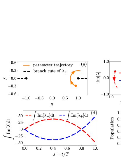
Figure 1: Open-trajectory evolution under Hamiltonian (8). The most growing state wins, in qualitative agreement with the naïve theory of Sec. II. This also agrees with the advanced theory of Sec. III, as the most growing state is also the end-point fastest growing one. (a) The trajectory in the parameter plane (orange) where the trajectory direction is shown with arrows and the orange dot depicts the starting point. The trajectory corresponds to the following parameters in Eq. (9): $\delta_{0}=0$, $g_{0}=1$, $R=0.3$, $T=500$, $\omega=-\pi/T$, $\phi=0.4\pi$. The black dots correspond to the EPs of the Hamiltonian, and the dashed lines correspond to the branch cuts of $\lambda_{\pm}$. (b) The trajectory of the eigenvalues $\lambda_{\pm}$ with arrows showing the trajectory direction. The eigevalues $\lambda_{\pm}$ at the start of the parameter trajectory are depicted as blue and red dots. (c) Riemann surface plot of $\mathrm{Im}\,\lambda_{\pm}(t)$ (red surface for $\lambda_{-}$, blue surface for $\lambda_{+}$). The state trajectory (black), with black dot depicting the starting point and the arrow showing the trajectory direction, corresponds to $\left|c_{+}(t)\right|^{2}\mathrm{Im}\,\lambda_{+}(t)+\left|c_{-}(t)\right|^{2}\mathrm{Im}\,\lambda_{-}(t)$. (d) The integrals $\mathrm{Im}\int_{0}^{t}dt\,\lambda_{\pm}(t)$ that govern the non-Hermitian state conversion under the naïve theory. (e) Population dynamics: the prediction of the naïve theory vs the numerical simulation. While qualitatively they agree — the state is ultimately converted to $\left|\psi_{+}\right\rangle$ — the location of the population switch is not the same ( $t_{1}\approx 0.8T$ vs $t_{1}^{\prime}\apprle 0.7T$).

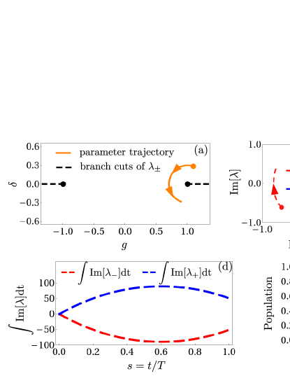
Figure 2: Open-trajectory evolution under Hamiltonian (8). The most growing state loses, in disagreement with the naïve theory of Sec. II. The end-point fastest growing state wins, in agreement with the advanced theory of Sec. III, which accounts for the errors of numerical simulation (in this example) and Hamiltonian control (in real experiments). (a) The trajectory in the parameter plane (orange) where the trajectory direction is shown with arrows and the orange dot depict the starting point. The trajectory corresponds to the following parameters in Eq. (9): $\delta_{0}=0$, $g_{0}=1$, $R=0.3$, $T=500$, $\omega=\pi/T$, $\phi=-0.6\pi$. The black dots correspond to the EPs of the Hamiltonian, and the dashed lines correspond to the branch cut of $\lambda_{\pm}$. (b) The trajectory of the eigenvalues $\lambda_{\pm}$ with arrows showing the trajectory direction. The eigevalues $\lambda_{\pm}$ at the start of the parameter trajectory are depicted as blue and red dots. (c) Riemann surface plot of $\mathrm{Im}\,\lambda_{\pm}(t)$ (red surface for $\lambda_{-}$, blue surface for $\lambda_{+}$). The state trajectory (black) , with black dot depicting the starting point and the arrow showing the trajectory direction, corresponds to $\left|c_{+}(t)\right|^{2}\mathrm{Im}\,\lambda_{+}(t)+\left|c_{-}(t)\right|^{2}\mathrm{Im}\,\lambda_{-}(t)$. (d) The integrals $\mathrm{Im}\int_{0}^{t}dt\,\lambda_{\pm}(t)$ that govern the non-Hermitian state conversion under the naïve theory. (e) Population dynamics: the prediction of the naïve theory vs the numerical simulation. The naïve theory predicts conversion to the most growing state $\left|\psi_{+}\right\rangle$, whereas the numerical simulation results in conversion to $\left|\psi_{-}\right\rangle$. The latter is in agreement with the advanced theory, as $\left|\psi_{-}\right\rangle$ is the end-point fastest growing state.

IV.1 Which state wins: the most growing vs the end-point fastest growing

We now discuss examples of how the naïve theory fails in quantitative (Fig. 1) and, most importantly, qualitative (Fig. 2) predictions for slow non-Hermitian evolution. We explain how the advanced theory gives the correct predictions.

Consider an open trajectory in the parameter space, cf. Fig. 1(a). Figure 1(b) shows the evolution of real and imaginary parts of $\lambda_{\pm}$ along the trajectory. As explained in Secs. II, III, the imaginary part $\mathrm{Im}\,\lambda_{\pm}$ is of key importance. Fig. 1(c) shows the state dynamics superimposed with the Riemann surface of $\lambda_{\pm}$. Namely, the black line shows $\left|c_{+}(t)\right|^{2}\mathrm{Im}\,\lambda_{+}(t)+\left|c_{-}(t)\right|^{2}\mathrm{Im}\,\lambda_{-}(t)$. One can see the typical feature of non-Hermitian state converison: starting in $\left|\psi_{-}\right\rangle$ with $\mathrm{Im}\,\lambda_{-}>0$, the system state adiabatically follows $\left|\psi_{-}\right\rangle$ until it suddenly switches to $\left|\psi_{+}\right\rangle$. The switch happens not immediately at the point at which $\mathrm{Im}\,\lambda_{-}=\mathrm{Im}\,\lambda_{+}=0$ (after which $\mathrm{Im}\,\lambda_{-}<0$ and $\mathrm{Im}\,\lambda_{+}>0$), but sometime later.

This can be qualitatively explained with the naïve theory of Sec. II, Eqs. (3–4). Indeed, Fig. 1(d) shows the evolution of $\int_{0}^{t}dt\,\mathrm{Im}\,\lambda_{\pm}(t)$. The integrals change their trends (growing/decreasing) at $t_{0}\approx 0.4T$, where $\mathrm{Im}\,\lambda_{-}=\mathrm{Im}\,\lambda_{+}=0$, however the amplification factors $\exp\left(\mathrm{Im}\int_{0}^{t}dt\,\lambda_{\pm}(t)\right)$ for the two states will only become equal at $t_{1}\approx 0.8T$, and soon after that, the population switch to $\left|\psi_{+}\right\rangle$ will happen.

The naïve theory, however, fails to explain the dynamics quantitatively, cf. Fig. 1(e). The numerical simulation shows that the population switch between $\left|\psi_{-}\right\rangle$ and $\left|\psi_{+}\right\rangle$ takes place at $t_{1}^{\prime}\apprle 0.7T$, i.e., significantly earlier than $\int_{0}^{t}dt\,\mathrm{Im}\,\lambda_{-}(t)=\int_{0}^{t}dt\,\mathrm{Im}\,\lambda_{+}(t)$. This can be explained by the advanced theory of Sec. II: The numerical simulation involes Trotterization of the evolution, which means that there is inherent error introduced every numerical time step $dt$. Interpreting this error as $\delta H(t)$ in Eq. (6), one can say that the error creates a small but finite population in $\left|\psi_{+}\right\rangle$. Similarly to the naïve theory, the population of $\left|\psi_{+}\right\rangle$ gets amplified once $t>t_{0}$. However, unlike in the naïve theory, the newly-created population of $\left|\psi_{+}\right\rangle$ does not need to overcome the suppression factor $\exp\left(\mathrm{Im}\int_{0}^{t_{0}}dt\,\left[\lambda_{+}(t)-\lambda_{-}(t)\right]\right)$ accumulated previously. This leads to the populations of $\left|\psi_{+}\right\rangle$ and $\left|\psi_{-}\right\rangle$ becoming equal at $t_{1}^{\prime}<t_{1}$.

A much more striking distinction between the predictions of the naïve and the advanced theories appears when one follows the same parameter trajectory in the reverse direction, cf. Fig. 2. Here the final state happens to be $\left|\psi_{-}\right\rangle$, and not $\left|\psi_{+}\right\rangle$, in contradiction with the naïve theory, cf. Fig. 2(e). This is, however, in agreement with the advanced theory, which predicts conversion to the end-point fastest growing state, which is $\left|\psi_{-}\right\rangle$: for $t_{0}\gtrsim 0.6T$, $\mathrm{Im}\,\lambda_{-}>0>\mathrm{Im}\,\lambda_{+}$, cf. Figs. 2(b, d). The mechanism is, again, the same: due to numerical errors, at every time step, a small fraction of population of $\left|\psi_{+}\right\rangle$ is converted to $\left|\psi_{-}\right\rangle$, whose population grows once $t_{0}\gtrsim 0.6T$; unlike in the naïve theory, the amplification factor does not need to overcome the huge suppression accumulated previously, $\exp\left(\mathrm{Im}\int_{0}^{t_{0}}dt\,\left[\lambda_{-}(t)-\lambda_{+}(t)\right]\right)$.

We strongly emphasize the following. One might think that numerical errors are an artifact of the simulation. That they can be eliminated with better numerical schemes and do not reflect experimental reality. In fact, quite the opposite stance should be taken. In a system with exponential instabilities, errors (however small) can lead to a qualitative change of behavior. Therefore, a better numerical scheme that reduces the uncontrolled errors, will not eliminate the reported effects as long as the evolution is sufficiently slow. That is, as long as the instabilities have enough time to grow and manifest. Similarly, any experimental implementation will necessarily have noise in the control parameters (even if tiny). Therefore, the behavior illustrated above — non-Hermitian evolution brings the system to the end-point fastest growing state, and not to the most growing one — is not an artifact, but is to be generically expected in the limit of slow evolution ($T\rightarrow\infty$).

IV.2 Non-chiral state conversion upon encircling the exceptional point

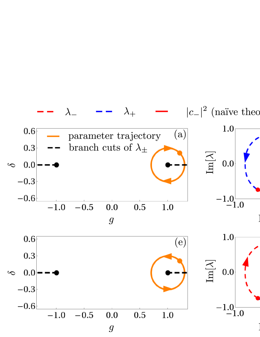
Figure 3: Non-chiral state conversion when encircling an exceptional point. The numerical result is in clear discrepancy with the predictions of the naïve theory. The advanced theory explains the numerical result, as $\left|\psi_{-}\right\rangle$ is the end-point fastest growing state for both encircling directions. (a) The trajectory for clockwise encircling in the parameter plane (orange) corresponds to the following parameters in Eq. (9): $\delta_{0}=0$, $g_{0}=1$, $R=0.3$, $T=500$, $\omega=-2\pi/T$, $\phi=-3\pi/4$. The trajectory direction is shown with arrows and the orange dot depict the starting point. The black dots correspond to the EPs of the Hamiltonian, and the dashed lines correspond to the branch cuts of $\lambda_{\pm}$. (b) The trajectory of the eigenvalues $\lambda_{\pm}$ corresponding to the clockwise trajectory. The eigevalues $\lambda_{\pm}$ at the start of the parameter trajectory are depicted as blue and red dots, and the arrows show the trajectory direction. (c) The population dynamics for clockwise encircling when the system is initialized in $\left|\psi_{-}\right\rangle$. (d) The population dynamics for clockwise encircling when the system is initialized in $\left|\psi_{+}\right\rangle$. (e) The trajectory for counterclockwise encircling in the parameter plane (orange) corresponds to the following parameters in Eq. (9): $\delta_{0}=0$, $g_{0}=1$, $R=0.3$, $T=500$, $\omega=2\pi/T$, $\varphi=-3\pi/4$. (f,g,h) Same as (b,c,d), but for the counterclockwise trajectory.

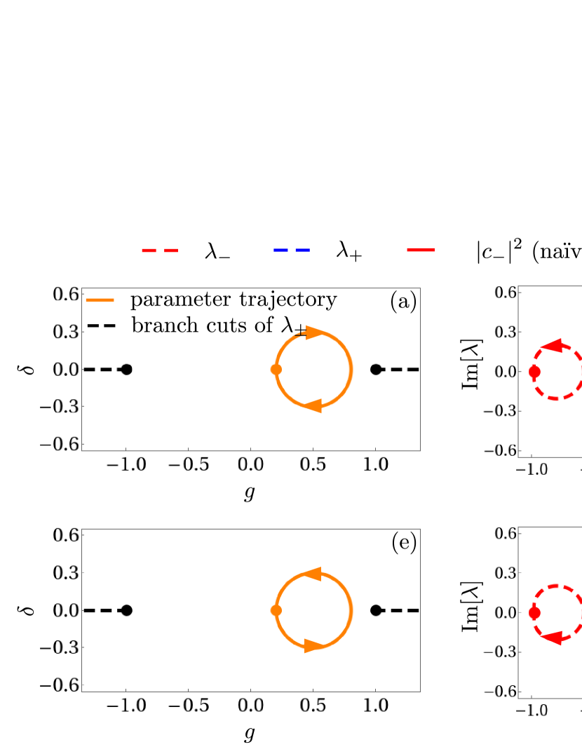
Figure 4: Chiral state conversion without encircling an exceptional point. The naïve theory predicts no conversion whatsoever, while the numerics predicts conversion to $\left|\psi_{-}\right\rangle$ ($\left|\psi_{+}\right\rangle$) for clockwise (counterclockwise) trajectory. This is explained by the advanced theory as the respective states are the end-point fastest growing in the respective cases. (a) The clockwise trajectory (orange) corresponds to the following parameters in Eq. (9): $\delta_{0}=0$, $g_{0}=0.5$, $R=0.3$, $T=500$, $\omega=-2\pi/T$, $\phi=0$. The trajectory direction is shown with arrows and the orange dot depict the starting point. The black dots correspond to the EPs of the Hamiltonian, and the dashed lines correspond to the branch cuts of $\lambda_{\pm}$. (b) The trajectory of the eigenvalues $\lambda_{\pm}$ corresponding to the clockwise trajectory. The eigevalues $\lambda_{\pm}$ at the start of the parameter trajectory are depicted as blue and red dots, and the arrows show the trajectory direction (c) The population dynamics for clockwise encircling when the system is initialized in $\left|\psi_{-}\right\rangle$. (d) The population dynamics for clockwise encircling when the system is initialized in $\left|\psi_{+}\right\rangle$. (e) The counterclockwise trajectory (orange) corresponds to the following parameters in Eq. (9): $\delta_{0}=0$, $g_{0}=0.5$, $R=0.3$, $T=500$, $\omega=2\pi/T$, $\varphi=0$. (f,g,h) Same as (b,c,d), but for the counterclockwise trajectory.

The convetional theoretical [49, 50, 51, 53, 55, 58, 64] and experimental [54, 26, 63, 66, 45, 12] expectation when ecircling an EP is for the state conversion to be chiral, i.e., dependent on the encircling direction. This is related to the non-analytic structure of the system eigenvalues $\lambda_{\pm}$ and eigenstates $\left|\psi_{\pm}\right\rangle$ at the EP [58]. However, there have also been theoretical [60] and experimental [59] reports about non-chiral behavior when encircling an EP, depending on the specific trajectory and/or its starting point.

Consider the trajectory that encircles an EP, as depicted in Figs. 3(a,e). The naïve theory predicts that for the clockwise encircling, essentially any initial state is converted into $\left|\psi_{+}\right\rangle$ (Figs. 3(c,d)), whereas for the counterclockwise one, essentially any initial state is converted into $\left|\psi_{-}\right\rangle$ (Figs. 3(g,h)). Which corresponds to the expected chiral behavior. However, the numerical curves in these panels tell a different story: for both encircling directions, numerical simulations predict conversion to $\left|\psi_{-}\right\rangle$ — the non-chiral behavior.

This behavior is easily explainable from our advanced theory. Notice that for both trajectories the end-point fastest growing state is $\left|\psi_{-}\right\rangle$, see Figs. 3(b,f). Therefore, the advanced theory predicts non-chiral conversion to $\left|\psi_{-}\right\rangle$, in agreement with the numerical simulations.

We note in passing that apart from numerical and experimental evidence, Ref. [59] provides analytical considerations to explain the non-chiral conversion, which — in contrast to our advanced theory — do not include fast noise in the course of evolution. These considerations turn out to be erroneous. By contrast, Ref. [60] provides a correct explanation — yet one specific to the trajectory considered in that work; this explanation is consistent with our advanced theory. We discuss these works in detail in Appendix B.

IV.3 Chiral state conversion without encircling the exceptional point

Another example of unconventional behavior concerns chiral conversion without encircling any EPs. Such behavior has been reported theoretically [56, 57] and experimentally [68].

Consider the trajectory depicted in Figs. 4(a,e). The naïve theory predicts no conversion whatsoever: if the system is initialized in $\left|\psi_{-}\right\rangle$, it ends up in $\left|\psi_{-}\right\rangle$ (Figs. 4(c,g)), and similarly for $\left|\psi_{+}\right\rangle$ (Figs. 4(d,h)). This is beacuse this trajectory is fine-tuned: it has $\mathrm{Im}\int_{0}^{T}dt\,\lambda_{\pm}(t)=0$. However, the numerical simulation predicts conversion to $\left|\psi_{-}\right\rangle$ for the clockwise trajectory (Figs. 4(c,d)) and to $\left|\psi_{+}\right\rangle$ for the counterclockwise one (Figs. 4(g,h)). Our advanced theory easily explains this: the respective states are the end-point fastest growing ones, as seen in Figs. 4(b,f).

Just as in the previous section, we note in passing that works [56, 57], apart from numerical studies, provided analytical arguments to explain this behavior within the framework of perfectly-controlled slow evolution. These arguments turn out to be erroneous and are discussed in detail in Appendix B.

V Demonstrating the quantitative accuracy of the advanced theory

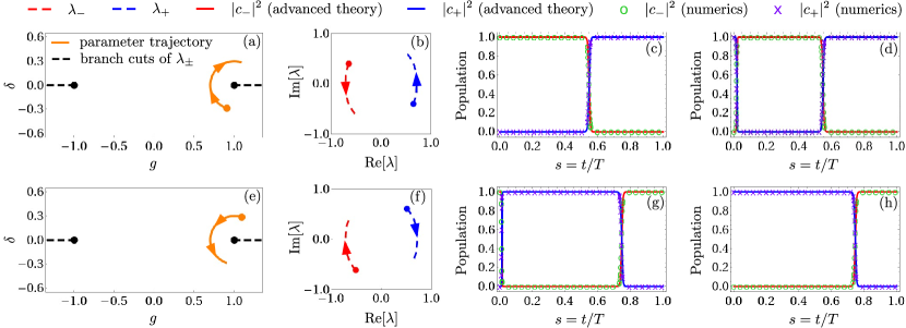
Figure 5: Open-trajectory evolution under the perturbed Hamiltonian $\bar{H}(t)$ (11). The parameter trajectories in panels (a) and (e) are identical to those in Fig. 1(a) and Fig. 2(a) respectively: $\delta_{0}=0$, $g_{0}=1$, $R=0.3$, $T=500$, $\omega=-\pi/T$, $\phi=0.4\pi$ for panel (a) and $\delta_{0}=0$, $g_{0}=1$, $R=0.3$, $T=500$, $\omega=\pi/T$, $\phi=-0.6\pi$ for panel (e). The trajectory direction is shown with arrows and the orange dot depict the starting point. Panels (b) and (f) show the evolution of the instantaneous eigenvalues of $\bar{H}(t)$. The eigevalues $\lambda_{\pm}$ at the start of the parameter trajectory are depicted as blue and red dots, and the arrows show the trajectory direction. Panels (c) and (g) show the population dynamics along the respective trajectories when starting in $\left|\psi_{-}\right\rangle$, while the panels (d) and (h) show the same when starting in $\left|\psi_{+}\right\rangle$. The evolutions in numerical simulations and as predicted by the advanced theory of Sec. III are in quantitative agreement.

In this section, we demonstrate that our advanced theory of Sec. III gives not only correct qualitative predictions, but is also capable of accurately predicting the quantitative behavior. We demonstrate this by considering time dynamics that corresponds to non-Hermitian conversion.

The advanced theory invokes fast perturbation on top of controlled slow evolution. As we have argued above, such perturbations will appear generically in experiments and in numerical simulations. However, in order to demonstrate quantitative accuracy, one needs to know the dominant source of perturbation. To this end, we consider the evolution under the Hamiltonian

$$\bar{H}(t)=H(t)+\varepsilon\delta H(t),$$ (11)

with $H(t)$ as defined in Eqs. (8–9) and

$$\delta H(t)=\begin{pmatrix}0&\cos\Omega t\\ \cos\Omega t&0\end{pmatrix}.$$ (12)

In the examples below, we choose $\varepsilon=10^{-4}$ and $\Omega=2\pi/5$. The choice of parameters is dictated by the following considerations. The perturbation size $\varepsilon$ is chosen small in order not to affect the instantaneous eigenstates and eigenvalues of $\bar{H}$ to any significant degree. The perturbation frequency $\Omega$ is chosen to be much larger than $\left|\omega\right|\leq 2\pi/T=2\pi/500$ ($\omega$ being the same as in Figs. 1–4). At the same time, $\Omega$ is chosen to be of the same order as the distance between the eigenvalues of $H(t)$, $\left|\lambda_{+}(t)-\lambda_{-}(t)\right|\sim 1$. This is done in order to ensure that $\varepsilon\delta H(t)$ is roughly resonant and thus is the dominant perturbation in our numerical simulations. Other, uncontrolled, perturbations are still inherently present in our numerical simulations due to time discretization. However, being close to resonant, the controlled perturbation $\varepsilon\delta H(t)$ is more important than the uncontrolled perturbations.

For our demonstration, we use the same parameter trajectories as considered in Sec. IV.1. The example of Fig. 1 considered evolution along an open trajectory without any controlled perturbations ($\varepsilon=0$). The naïve theory of Sec. II was able to predict the outcome of the evolution qualitatively, however, the time at which the population switch takes place was predicted incorrectly. The same trajectory is used for Figs. 5(a–d), now including the controlled perturbation (11–12). By comparing Fig. 5(b) with Fig. 1(b), one sees that the perturbation $\varepsilon\delta H(t)$ does not have any noticeable effect on the Hamiltonian eigenvalues. At the same time the population switch in the numerical simulation now takes place at $t_{1}^{\prime\prime}<0.6T$ (cf. Figs. 5(c,d)), as opposed to $t_{1}^{\prime}>0.6T$ in Fig. 1(e). This shows that the perturbation $\varepsilon\delta H(t)$ of Eq. (12) has a noticeable impact on the evolution, stronger than the numerical errors. Using the theory of Sec. III, Eq. (6), we calculate the evolution of state populations, as presented in Figs. 5(c,d). One sees that the numerical simulation and the predictions of our advanced theory are in very good quantitative agreement.

The same applies for the reversed trajectory. Figure 2 showed a population switch at $t_{1}^{\prime}>0.8T$, which is not predicted at all by the naïve theory that assumes perfectly-controlled slow evolution. We explained in Sec. IV.1 how the advanced theory qualitatively predicts this reversal by highlighting the role of the end-point fastest growing state (as opposed to the most growing state). Figures 5(e–h) show that the advanced theory also captures the dynamics quantitatively. Again, despite no noticeable effect on the eigenvalues in Fig. 5(f) compared to Fig. 2(b), the manually added perturbation $\varepsilon\delta H(t)$ provokes the population switch at $t_{1}^{\prime\prime}<0.8T$, cf. Figs. 5(g,h). As $t_{1}^{\prime\prime}<t_{1}^{\prime}$, this shows the dominance of $\varepsilon\delta H(t)$ over numerical errors. And the result of numerical simulations is in a very good quantitative agreement with the predictions of the advanced theory, cf. Figs. 5(g,h).

We provide details on how the advanced theory curves have been produced and also further examples of quantitative agreement between the advanced theory and the numerical simulations in Appendix C. There we consider closed evolution trajectories associated with chiral and non-chiral non-Hermitian state conversion.

VI Proposals for experimental verification

Below we list a few paradigmatic tests of our theory, that may be relevant for various experimental platforms.

Recent experiments [68] have demonstrated chiral state transfer when not encircling an EP. Our theory predicts that the conversion result is determined by the eigenvalues of the non-Hermitian Hamiltonian towards the end of the evolution. This implies that simply changing the starting point on the same closed trajectory in the parameter space can change the conversion behavior from chiral to non-chiral, cf. Figs. 8 and 9 in Appendix C.

More delicate tests of our theory are possible by changing the evolution speed while still staying within the applicability domain of the theory. Let us assume that the strength and spectrum of noise do not depend on details of the controlled evolution. Our theory indicates that depending on the speed of the controlled evolution during different segments of the trajectory (e.g., on the evolution time $T$), the populations of different eigenmodes introduced by the noise will or will not have enough time to grow, following the analysis of Sec. III. When the predictions of our naïve (no noise) and advanced (high-frequency noise) theories differ, one can switch between the two behaviors by appropriately choosing $T$ (so that the noise-induced perturbations do or do not have ample time to be amplified).

Further test of our theory would be to compare runs with the same initial and final Hamiltonian parameters, but different trajectories in parameter space. In the appropriate limit (full-fledged noise-induced perturbations), the final state should not depend on the trajectory.

Finally, in order to verify the quantitative accuracy of our theory, one could controllably add noise to the system evolution. Making sure that the controlled noise is dominant over the environmental influences, one could predict the time dynamics quantitatively, similarly to what was done in Sec. V.

VII Conclusions

Here we have presented a general comprehensive analytic approach for analyzing slow non-Hermitian dynamics. Our theory comprises two layers. We first address controllable slow non-Hermitian evolution. We next add the effect of fast perturbations on top of the slow evolution. This is a classical way of modeling of high-frequency-noise components that represent coupling to environment. They are expected both in experiments and in numerical simulations. Combined with inherent exponential instabilities of non-Hermitian systems, this second layer of our theory becomes indispensable when it comes to non-Hermitian dynamics and radically changes the expected behaviors.

The resulting description greatly simplifies the analysis of such systems. Simulating the full slow evolution along a certain trajectory in the Hamiltonian’s parameter space is no more needed to infer the end state. Instead, the resulting state of the system is determined by the final point in parameter space. It is insensitive to the trajectory traversed and its time dependence. To experimentally test our theory one may design different trajectories that end up at the same point in parameter space and compare the resulting states.

We have applied our theory to analyze the effect of non-Hermitian state conversion with a special focus on its chirality. We have shown that our theory allows for predicting the conversion chirality qualitatively, explaining all the known behaviors. We have further shown that given the knowledge of the dominant fast perturbation, our theory produces quantitatively accurate predictions for the specific conversion times. Ultimately, we have shown that the chirality of slow non-Hermitian state conversion in the real world is not related to the physics of EPs. Instead, it is determined by the system’s decay rate spectrum at the ends of the evolution trajectory. Hence the chiral state conversion is non-topological. This provides a simple example of how beautiful mathematical constructions (the relation between the non-analiticity at exceptional points and chiral non-Hermitian state conversion) are washed out by the “stern realities of life”, i.e., noise.

In practical terms, our theory advances the understanding of slow non-Hermitian dynamics. The clear intuitive picture it provides can simplify simulations and design of devices involving few- and many-body, quantum and classical non-Hermitian systems. Our theory is straightforward to generalize to more complex descriptions of open systems, such as quantum systems governed by Lindbladians or hybrid Liouvillians.

Code availability

The Wolfram Mathematica code used to produce the Figures of the manuscript and the respective simulations can be found on a GitHub repostory [88].

Appendix A Derivation of analytical results

In this Appendix, we provide derivations of our general results for slow non-Hermitian evolution, which we have concisely presented in Secs. II and III. Section A.1 focuses on the case of genuine slow evolution, whereas Sec. A.2 considers the effect of uncontrolled fast noise. We emphasize that the results of this Appendix are valid for arbitrary trajectories in the parameter space (closed or open) as long, as the evolution is sufficiently smooth and no exceptional points or degeneracy points lie exactly on the trajectory.

A.1 Iterative adiabatic expansion

A.1.1 Idea and first orders

Consider a time-dependent Hamiltonian $H(t)=H_{s}$ with $s=t/T\in[0,1]$. The Hamiltonian may be Hermitian or non-Hermitian and is time-dependent. The values it takes at the initial and final moments of the evolution are $H(t=0)=H_{0}$ and $H(t=T)=H_{1}$, and the parameter $T\rightarrow\infty$ determines the speed of changing one Hamiltonian into another along a fixed sequence of Hamiltonians $H_{s}$. We assume that there are no exceptional or degeneracy points on the evolution trajectory, that is, at all $t\in[0,T]$ the Hamiltonian $H(t)$ can be diagonalised:

$$H(t)\equiv H_{s}=U(t)D(t)U^{-1}(t)\equiv U_{s}D_{s}U_{s}^{-1},$$ (13)

with $D(t)\equiv D_{s}$ being a diagonal matrix with all diagonal entries distinct. The diagonal entries of $D(t)$ are the Hamiltonian eigenvalues $\lambda_{n}(t)\equiv\lambda_{n,s}$. The matrix $U(t)\equiv U_{s}$ encodes the right eigenvectors of the Hamiltonian, $\left|n(t)\right\rangle=\left|n_{s}\right\rangle=U_{s}\left|n\right\rangle$, where $\left|n\right\rangle$ is a column vector $\left(0,\ldots,0,1,0,\ldots 0\right)^{\mathrm{T}}$ with $1$ on the $n$th postition.

The system state $\left|\psi(t)\right\rangle$ obeys the Schrödinger equation

$$i\partial_{t}\left|\psi(t)\right\rangle=H(t)\left|\psi(t)\right\rangle.$$ (14)

Our task is to express the final state $\left|\psi(T)\right\rangle$ through the initial state $\left|\psi(0)\right\rangle$ in the limit of $T\rightarrow\infty$. In order to explicitly keep track of the powers of $T$, we switch to the variable $s$. We define $\left|\psi(s=t/T)\right\rangle\equiv\left|\psi(t)\right\rangle$. Note that the quantities with $s$ as a subscript do not depend on $T$, whereas the evolution of $\left|\psi(s)\right\rangle$ does implicitly depend on $T$ (thence the difference in notation). The Schrödinger equation now looks

$$i\partial_{s}\left|\psi(s)\right\rangle=TH_{s}\left|\psi(s)\right\rangle.$$ (15)

The natural first step for solving this evolution is to work in the eigenbasis of $H_{s}$. Define $\left|\varphi(s)\right\rangle=U_{s}^{-1}\left|\psi(s)\right\rangle$. Then

$$i\partial_{s}\left|\varphi(s)\right\rangle=T\left[D_{s}-X^{(1)}(s)\right]\left|\varphi(s)\right\rangle,$$ (16)

where $X^{(1)}(s)=\frac{1}{T}iU_{s}^{-1}\partial_{s}U_{s}$. Note that the term involving $X^{(1)}(s)$ is small compared to the leading term $D_{s}$. The smallness of $X^{(1)}$, however, does not allow one to neglect it, as its contribution over the evolution of duration $T$ may be finite.

In order to arrive at a controllable approximation, introduce $V_{1}(s)$ that diagonalizes $D_{s}-X^{(1)}(s)$:

$$D_{s}-X^{(1)}(s)=V_{1}(s)\Delta_{1}(s)\left[V_{1}(s)\right]^{-1},$$ (17)

and

$$\left|\varphi_{1}(s)\right\rangle=\left[V_{1}(s)\right]^{-1}\left|\varphi(s)\right\rangle.$$ (18)

Here $\Delta_{1}(s)=D_{s}+D^{(1)}(s)$ is diagonal. Within the perturbation theory in $X^{(1)}$, one finds that

$$V_{1}(s)=\mathbb{I}+W^{(1)}(s),$$ (19)

$$W^{(1)}(s)=\sum_{m\neq n}\left|m\right\rangle\frac{\left\langle m\right|X^{(1)}(s)\left|n\right\rangle}{\lambda_{m,s}-\lambda_{n,s}}\left\langle n\right|+O\left(T^{-2}\right)$$ (20)

and

$$D^{(1)}(s)=\sum_{n}\left|n\right\rangle\lambda_{n}^{(1)}(s)\left\langle n\right|,$$ (21)

$$\lambda_{n}^{(1)}(s)=-\left\langle n\right|X^{(1)}(s)\left|n\right\rangle+O\left(T^{-2}\right).$$ (22)

Then

$$i\partial_{s}\left|\varphi_{1}(s)\right\rangle=T\left[\Delta_{1}(s)-X^{(2)}(s)\right]\left|\varphi_{1}(s)\right\rangle,$$ (23)

where $X^{(2)}(s)=\frac{1}{T}i\left[V_{1}(s)\right]^{-1}\partial_{s}V_{1}(s)$. Note that $\partial_{s}V_{1}(s)=\partial_{s}W^{(1)}(s)\propto 1/T$, so that $X^{(2)}(s)=O\left(T^{-2}\right)$. Therefore, one can neglect the contribution of $X^{(2)}(s)$ for the evolution of duration $T$ and approximately write

$$i\partial_{s}\left|\varphi_{1}(s)\right\rangle\approx T\Delta_{1}(s)\left|\varphi_{1}(s)\right\rangle,$$ (24)

which is immediately solved by

$$\left|\varphi_{1}(s)\right\rangle=\exp\left(-iT\int_{0}^{s}d\sigma\Delta_{1}(\sigma)\right)\left|\varphi_{1}(0)\right\rangle.$$ (25)

Note that the time ordering in the exponential is unnecessary since $\Delta^{(1)}(\sigma)$ is always diagonal.

The solution for $\left|\varphi(s)\right\rangle$ follows immediately as

$$\left|\varphi(s)\right\rangle=V_{1}(s)\exp\left(-iT\int_{0}^{s}d\sigma\Delta_{1}(\sigma)\right)\left[V_{1}(0)\right]^{-1}\left|\varphi(0)\right\rangle.$$ (26)

Applying this formula for $s=1$ (i.e., $t=T$), one finds

$$\left|\varphi(s=1)\right\rangle=\exp\left(-iT\int_{0}^{1}d\sigma\Delta_{1}(\sigma)\right)\left|\varphi(0)\right\rangle\\ +W^{(1)}(1)\exp\left(-iT\int_{0}^{1}d\sigma\Delta_{1}(\sigma)\right)\left|\varphi(0)\right\rangle\\ +\exp\left(-iT\int_{0}^{1}d\sigma\Delta_{1}(\sigma)\right)W^{(1)}(0)\left|\varphi(0)\right\rangle\\ +O\left[T^{-2}\exp\left(-iT\int_{0}^{1}d\sigma\Delta_{1}(\sigma)\right)\right].$$ (27)

In the exponentials, $T\int_{0}^{1}d\sigma\Delta_{1}(\sigma)=T\int_{0}^{1}d\sigma D(\sigma)+T\int_{0}^{1}d\sigma D^{(1)}(\sigma)$. $D(s)\propto T^{0}$, so the first integral is proportional to $T$, whereas the integral of $D^{(1)}(t)$ is proportional to $T^{0}$ and can be neglected.

This leads us to the final formula,

$$\left|\varphi(s=1)\right\rangle\approx\exp\left(-iT\int_{0}^{1}d\sigma D(\sigma)\right)\left|\varphi(0)\right\rangle\\ +W^{(1)}(1)\exp\left(-iT\int_{0}^{1}d\sigma D(\sigma)\right)\left|\varphi(0)\right\rangle\\ +\exp\left(-iT\int_{0}^{1}d\sigma D(\sigma)\right)W^{(1)}(0)\left|\varphi(0)\right\rangle.$$ (28)

Let us discuss the meaning of the three terms in this expression.

The first term corresponds to the conventional adiabatic approximation: each eigenstate of the instantaneous Hamiltonian evolves with the respective eigenvalue. In the case of a Hermitian $H_{s}$, $D(\sigma)$ is always real, so that each eigenstate simply accumulates the dynamic phase (and the geometric phase would be given by $T\int_{0}^{1}d\sigma D^{(1)}(\sigma)$ in Eq. (27), which we neglected in Eq. (28)). In the non-Hermitian case, the diagonal entries of $D(\sigma)$ may have an imaginary part, corresponding to some states growing and some decaying. Therefore, for sufficiently large $T$, one expects this term to align with the most growing (least decaying) eigenstate, i.e., the state $\left|n_{s=1}\right\rangle$, for which the integral of the growth rate over the entire trajectory, $\mathrm{\mathrm{Im}\,}\int_{0}^{1}ds\lambda_{n,s}$, is the largest. If, however, the most growing state has zero amplitude in the intial state $\left|\varphi(0)\right\rangle$, then this term aligns with the second most growing state (unless the amplitude of this state is also zero, and so on).

The second term in Eq. (28) tells that due to finite $T$, the adiabatic limit is violated, and the final state $\left|\varphi(s=1)\right\rangle$ is only equal to the most growing eigenstate up to $O(T^{-1})$ corrections. Finally, the last term implies that due to adiabaticity violation at the beginning of the evolution, population of all $\left|n_{s=0}\right\rangle$ is generically generated, and therefore the above remark concerning the amplitudes in the initial state is insignificant: generically, for sufficiently large $T$, the state $\left|\varphi(s=1)\right\rangle$ aligns with the most growing among the eigenstates $\left|n_{s=1}\right\rangle$.

Equation (28) thus predicts and describes the non-Hermitian state conversion: essentially any initial state under slow non-Hermitian evolution gets converted into the most growing eigenstate. All the other states are suppressed. Naïvely, one expects this suppression to be exponential in $T$. However, the conversion accuracy is only $O(T^{-1})$ due to adiabaticity violation at the end of the evolution.

A.1.2 Solution to an arbitrary order

Having demonstrated in Sec. A.1.1 that the lowest order of the adiabatic expansion captures the physics of the non-Hermitian state conversion, we are now in a position to develop a systematic expansion in powers of $T$ and demonstrate that further orders do not bring qualitative changes. Instead of neglecting $X^{(2)}$ in Eq. (23), define $V_{2}(s)$ that diagonalizes $\Delta_{1}(s)-X^{(2)}(s)$:

$$\Delta_{1}(s)-X^{(2)}(s)=V_{2}(s)\Delta_{2}(s)\left[V_{2}(s)\right]^{-1},$$ (29)

and

$$\left|\varphi_{2}(s)\right\rangle=\left[V_{2}(s)\right]^{-1}\left|\varphi_{1}(s)\right\rangle.$$ (30)

Here $\Delta_{2}(s)=\Delta_{1}(s)+D^{(2)}(s)$ is diagonal. Within the perturbation theory in $X^{(2)}$, one finds that

$$V_{2}(s)=\mathbb{I}+W^{(2)}(s),$$ (31)

$$W^{(2)}(s)=\sum_{m\neq n}\left|m\right\rangle\frac{\left\langle m\right|X^{(2)}(s)\left|n\right\rangle}{\lambda_{m,s}-\lambda_{n,s}}\left\langle n\right|+O\left(T^{-3}\right)$$ (32)

and

$$D^{(2)}(s)=\sum_{n}\left|n\right\rangle\lambda_{n}^{(2)}(s)\left\langle n\right|,$$ (33)

$$\lambda_{n}^{(2)}(s)=-\left\langle n\right|X^{(2)}(s)\left|n\right\rangle+O\left(T^{-3}\right).$$ (34)

Then

$$i\partial_{s}\left|\varphi_{2}(s)\right\rangle=T\left[\Delta_{2}(s)-X^{(3)}(s)\right]\left|\varphi_{2}(s)\right\rangle,$$ (35)

where $X^{(3)}(s)=\frac{1}{T}i\left[V_{2}(s)\right]^{-1}\partial_{s}V_{2}(s)$. Note that $\partial_{s}V^{(1)}(s)=\partial_{s}W^{(2)}(s)\propto 1/T^{2}$, so that $X^{(3)}(s)=O\left(T^{-3}\right)$.

Similarly, one can iteratively define for any order $k$

$$\left|\varphi_{k}(s)\right\rangle=\left[V_{k}(s)\right]^{-1}\left|\varphi_{k-1}(s)\right\rangle\\ =\left[V_{k}(s)\right]^{-1}\ldots\left[V_{1}(s)\right]^{-1}\left|\varphi(s)\right\rangle,$$ (36)

obeying

$$i\partial_{s}\left|\varphi_{k}(s)\right\rangle=T\left[\Delta_{k}(s)-X^{(k)}(s)\right]\left|\varphi_{k}(s)\right\rangle,$$ (37)

with

$$X^{(k)}(s)=\frac{1}{T}i\left[V_{k-1}(s)\right]^{-1}\partial_{s}V_{k-1}(s)=O\left(T^{-k}\right).$$ (38)

The matrices $V_{k}(s)$ are defined as diagonalisers of $\Delta_{k-1}(s)-X^{(k-1)}(s)$:

$$\Delta_{k-1}(s)-X^{(k-1)}(s)=V_{k}(s)\Delta_{k}(s)\left[V_{k}(s)\right]^{-1},$$ (39)

$$\Delta_{k}(s)=\Delta_{k-1}(s)+D^{(k)}(s),\quad D^{(k)}=O\left(T^{-k}\right),$$ (40)

$$V_{k}(s)=\mathbb{I}+W^{(k)}(s),\quad W^{(k)}(s)=O\left(T^{-k}\right).$$ (41)

Note that we mark the objects of order $T^{-k}$ by the superscript $(k)$, such as $X^{(k)}$ or $W^{(k)}$, whereas other objects appearing at $k$th iteration and having subscript $k$, like $V_{k}$, are not small.

Neglecting the small term $X^{(k)}(s)\sim T^{-k}$ in Eq. (37), one then obtains that

$$\left|\varphi(s)\right\rangle\approx U_{k}(s)\exp\left(-iT\int_{0}^{s}d\sigma\Delta_{k}(\sigma)\right)\left[U_{k}(0)\right]^{-1}\left|\varphi(0)\right\rangle,$$ (42)

$$U_{k}(s)=V_{1}(s)V_{2}(s)\ldots V_{k}(s)=\mathbb{I}+W_{k}(s),$$ (43)

$$\left[U_{k}(s)\right]^{-1}=\left[V_{k}(s)\right]^{-1}\ldots\left[V_{2}(s)\right]^{-1}\left[V_{1}(s)\right]^{-1}=\mathbb{I}+\tilde{W}_{k}(s),$$ (44)

Therefore,

$$\left|\varphi(s=1)\right\rangle=\exp\left(-iT\int_{0}^{1}d\sigma\Delta_{k}(\sigma)\right)\left|\varphi(0)\right\rangle\\ +W_{k}(1)\exp\left(-iT\int_{0}^{1}d\sigma\Delta_{k}(\sigma)\right)\left|\varphi(0)\right\rangle\\ +\exp\left(-iT\int_{0}^{1}d\sigma\Delta_{k}(\sigma)\right)\tilde{W}_{k}(0)\left|\varphi(0)\right\rangle\\ +W_{k}(1)\exp\left(-iT\int_{0}^{1}d\sigma\Delta_{k}(\sigma)\right)\tilde{W}_{k}(0)\left|\varphi(0)\right\rangle\\ +O\left(T^{-k-1}\exp\left(-iT\int_{0}^{1}d\sigma\Delta_{k}(\sigma)\right)\right).$$ (45)

Notice that $\Delta_{k}(s)=D(s)+O\left(T^{-1}\right)$, so the physics described by this formula is the same as the one of Eq. (28). The only significant difference is the appearance of the fourth term, involving both $W_{k}$ and $\tilde{W}_{k}$, each of which is $O(T^{-1})$. This term shows that the non-Hermitian conversion is never exponentially perfect but is only accurate up to $O(T^{-1})$ corrections due to non-adiabaticity at the end of the trajectory — something hinted at already by the second term in Eq. (28).

A.1.3 Convergence and errors

Remark that the solution (45) is valid to order $T^{-k}$ for arbitrary $k$, and is therefore asymptotically exact. It is important to note, however, that the iterations do not necessarily converge to the exact solution as $k\rightarrow\infty$. I.e., our expansion may be an asymptotic expansion, but not a convergent one.

In order to appreciate the difference, consider the Landau-Zener problem for Hermitian Hamiltonians [90, 91, 92, 93, 94]. Consider a two-level Hamiltonian

$$H(t)=\begin{pmatrix}\frac{1}{2}\lambda t&\eta\\ \eta&-\frac{1}{2}\lambda t\end{pmatrix}$$ (46)

controlling the system evolution from $t=-t_{0}/2$ until $t=t_{0}/2$; we take $\lambda>0$ and $\eta>0$ for simplicity. For the evolution time $t_{0}\rightarrow\infty$ the initial state $\left(1,0\right)^{\mathrm{T}}$ (which is the ground state at $t\rightarrow-\infty$) may become at $t\rightarrow\infty$ the new ground state $\left(0,1\right)^{\mathrm{T}}$ or the excited state $\left(1,0\right)^{\mathrm{T}}$. The latter happens with the Landau-Zener probability $P_{\mathrm{LZ}}=\exp\left(-2\pi\eta^{2}/\lambda\right)$ [90, 91, 92, 93, 94]. The speed of evolution is controlled by $\lambda$. In particular, for $\lambda\rightarrow 0$, $P_{\mathrm{LZ}}$ vanishes, in agreement with the adiabatic theorem. For small but finite $\lambda$, $P_{\mathrm{LZ}}$ is exponentially small and is non-analytic as $\lambda\rightarrow 0$.

Now compare this to the predictions of Eq. (45). In order to make a link with our definitions, introduce $E_{0}=\lambda t_{0}$, $T=t_{0}$, and take the limit of $t_{0}\rightarrow\infty$ such that $E_{0}=\mathrm{const}$. That is, $\lambda=E_{0}/t_{0}\rightarrow 0$ and $T=E_{0}/\lambda\rightarrow\infty$. The matrix diagonalizing the Hamiltonian (46) is $U(t)\equiv U_{s}=\mathbb{I}+O(\eta/E_{0})$, cf. Eq. (13). Therefore, $W_{k}(1)$ and $\tilde{W}_{k}(0)$ in Eq. (45) are $\propto\eta/E_{0}$, so that in the Landau-Zener limit $E_{0}\rightarrow\infty$, the equation predicts vanishing probability up to corrections of order $T^{-k-1}$ for any $k$. On one hand, this is consistent with the exact Landau-Zener result $P_{\mathrm{LZ}}=\exp\left(-.../\lambda\right)=\exp\left(-...T\right)$. On the other hand, expansion (45) does not enable one to obtain the exponentially small answer.

Two remarks are due in relation to the above comparison. First, we have deliberately avoided a discussion of the order of limits above. However, a proper rewriting of the Landau-Zener formula in the newly-defined units, $P_{\mathrm{LZ}}=\exp\left(-2\pi\eta^{2}T/E_{0}\right)$, hints that the exact way of taking limits $\eta T\rightarrow\infty$ and $E_{0}/\eta\rightarrow\infty$ is important. The ways they are taken in the Landau-Zener problem ($E_{0}\rightarrow\infty$ while keeping $E_{0}/T$ constant) and in the derivation of expansion (45) (first $T\rightarrow\infty$, and then $E_{0}\rightarrow\infty$) are different. Therefore, the above comparison to the Landau-Zener problem only serves to illustrate the possibility of effects not captured by our expansion, but not to prove their existence.

Second, when considering finite $E_{0}$ (equivalently, finite $t_{0}$), the Landau-Zener formula aqcuires corrections, which are power-law in $T$ [95, 96, 97, 98, 99]. We expect our expansion to work in this setting. However, we have not investigated this problem in detail.

We note in passing that a number of works have investigated non-Hermitian Landau-Zener problems [80, 100]. Further, some recent works considered Hermitian Landau-Zener problems in the presence of Lindbladian terms [22, 24, 30].

A.1.4 Subtleties

Here we emphasize a few subtleties which do not influence the validity of Eq. (45), yet should be taken into account when interpreting its implications.

Corrections to non-Hermitian state conversion. The first and third terms in Eq. (45) describe non-Hermitian state conversion. Non-adiabaticity at the beginning of the evolution leads to generating amplitudes on all the instantaneous eigenstates. Then due to the eigenvalues having an imaginary part, the final state aligns with the most growing eigenstate $\left|n_{s}\right\rangle$ as $T\rightarrow\infty$. Based on these two terms, one may conclude that the conversion is exponentially accurate, and the contributions of other eigenstates are suppressed by factors of $\exp(-\ldots T)$. The second and fourth terms, however, clearly show that the non-adiabaticity at the end of the evolution generates transitions from the most growing eigenstate $\left|n_{s}\right\rangle$ to other eigenstates $\left|m_{s}\right\rangle$. Given that $W_{k}$ is generically $\propto T^{-1}$, this means that the conversion is only power-law accurate. This has been previously pointed out in Ref. [64].

Non-generic Hamiltonians. The above interpretation of conversion is based on the assumtion that the matrix $\tilde{W}_{k}(0)$ has all off-diagonal matrix elements non-zero, i.e., the non-adiabaticity at the beginning of the evolution generates components on all instantaneous eigenstates of the Hamiltonian. While generically true, this may not be the case for Hamiltonians featuring a special structure. For example, if $H_{s}$ admits a symmetry $\mathcal{S}$, $\left[H_{s},\mathcal{S}\right]=0$ for all “times” $s$, then all the matrix elements of $\tilde{W}_{k}(0)$ connecting states in different symmetry sectors will vanish. I.e., the conversion will happen to the most growing state within the symmetry sector. Similarly, if the Hamiltonian concerns two distinct subsystems (i.e., $H_{s}=H_{1,s}\otimes\mathbb{I}+\mathbb{I}\otimes H_{2,s}$) and the evolution concerns only one of them ($H_{2,s}\equiv H_{2,0}$), the conversion will only concern the part of the state related to the first system, while the second component of the state will remain intact.

A.2 The effect of fast noise

The consideration of Sec. A.1 assumed a controlled adiabatic evolution. However, in practice the evolution is never perfectly controlled due to systematic deviations and noise in the system parameters. Non-Hermitian systems feature exponential instabilities, making it mandatory to investigate the effect of such imperfections. Systematic imperfections and noise that is adiabatically slow, do not generate qualitatively new effects. They can be incorporated into the theory of Sec. A.1 as part of the system Hamiltonian. At most, they may change the specific form of the eigenstates and which of the eigenstates grows the most over the course of the evolution.

In contrast non-adiabatic noise may lead to qualitatively new effects by generating non-adiabatic transitions amidst the evolution. Below we show that this leads to a qualitative change: it is not the most growing state that wins in the course of the evolution, but the state that grows the last along the trajectory (cf. Sec. III). Below we derive the theory of non-Hermitian state conversion in the presence of fast (non-adiabatic) noise and explain its implications.

A.2.1 Derivation

In Sec. A.1, we have shown that the evolution under time-dependent Hamiltonian $H(t)=H_{s}$ with $s=t/T\in[0,1]$ for $T\rightarrow\infty$ is governed by the operator

$$\mathcal{U}(T,0)=\mathcal{T}\exp\left(-i\int_{0}^{T}dt\,H(t)\right)\\ =U(T)\mathcal{E}(T,0)U^{-1}(0),$$ (47)

$$\mathcal{E}(T,0)=\exp\left(-iT\int_{0}^{1}d\sigma\Delta_{k}(\sigma)\right)\\ +W_{k}(1)\exp\left(-iT\int_{0}^{1}d\sigma\Delta_{k}(\sigma)\right)\\ +\exp\left(-iT\int_{0}^{1}d\sigma\Delta_{k}(\sigma)\right)\tilde{W}_{k}(0)\\ +W_{k}(1)\exp\left(-iT\int_{0}^{1}d\sigma\Delta_{k}(\sigma)\right)\tilde{W}_{k}(0)\left|\varphi(0)\right\rangle\\ +O\left(T^{-k-1}\exp\left(-iT\int_{0}^{1}d\sigma\Delta_{k}(\sigma)\right)\right),$$ (48)

where $U(t)$ encodes the instantaneous eigenbasis of $H(t)$, cf. Eq. (13), $\Delta_{k}(s)=D_{s}+O\left(T^{-1}\right)$ are diagonal matrices $D_{s}$ encoding the instantaneous eigenvalues $\lambda_{n}(t)=\lambda_{n,s}$ of $H(t)$ plus some unimportant non-adiabatic corrections, $W_{k}(s)$ and $\tilde{W}_{k}(s)$ encode the non-adiabatic effects of eigenbasis evolution along the trajectory, and the form of $\mathcal{E}(T,0)$ is readily inferred from Eq. (45). The operator $\mathcal{U}(T,0)$ predicts conversion of essentially any initial state into one specific eigenstate $\left|n(T)\right\rangle$ of $H(T)$ in the limit $T\rightarrow\infty$; the final eigenstate $\left|n\right\rangle$ is the state that has the largest integral $\mathrm{Im}\int_{0}^{1}d\sigma\lambda_{n,\sigma}$ — that is, the eigenstate that grows the most over the course of the evolution.

Consider now the evolution generated by $\bar{H}(t)=H(t)+\varepsilon\delta H(t)$, where $\delta H(t)$ is a correction to the Hamiltonian due to imperfect control of the system parameters and $\varepsilon\ll 1$ controls its smallness. If this correction can be incorporated in the framework of slow evolution, such that one can write $\bar{H}(t=sT)=\bar{H}_{s}$, the predictions of Eqs. (52–53) hold: there is conversion to the most growing eigenstate of $\bar{H}$. The adiabatic perturbation may change the exact form of the eigenstate or may change which of the eigenstates wins. In contrast, we are interested in the effect of fast perturbations, which cannot be incorporated into the framework of iterative adiabatic expansion of Sec. A.1.

We are interested in calculating the evolution operator

$$\mathcal{\bar{U}}(T,0)=\mathcal{T}\exp\left(-i\int_{0}^{T}dt\,\bar{H}(t)\right),$$ (49)

which under the perturbation theory in $\delta H(t)$ can be expressed as

$$\mathcal{\bar{U}}(T,0)=\mathcal{U}(T,0)\\ -i\varepsilon\int_{0}^{T}dt_{1}\mathcal{U}(T,t_{1})\delta H(t_{1})\mathcal{U}(t_{1},0)\\ -\varepsilon^{2}\int_{0}^{T}dt_{2}\int_{0}^{t_{2}}dt_{1}\mathcal{U}(T,t_{2})\delta H(t_{2})\mathcal{U}(t_{2},t_{1})\delta H(t_{1})\mathcal{U}(t_{1},0)\\ +O\left(\varepsilon^{3}\right),$$ (50)

where

$$\mathcal{U}(t_{2},t_{1})=\mathcal{T}\exp\left(-i\int_{t_{1}}^{t_{2}}dt\,H(t)\right).$$ (51)

Applying the result of Sec. A.1 to the evolution between $t_{1}=s_{1}T$ and $t_{2}=s_{2}T$, one can write that

$$\mathcal{U}(t_{2},t_{1})=U(t_{2})\mathcal{E}(t_{2},t_{1})U^{-1}(t_{1}),$$ (52)

$$\mathcal{E}(t_{2},t_{1})=\exp\left(-iT\int_{s_{1}}^{s_{2}}d\sigma\Delta_{k}(\sigma)\right)\\ +W_{k}(s_{2})\exp\left(-iT\int_{s_{1}}^{s_{2}}d\sigma\Delta_{k}(\sigma)\right)\\ +\exp\left(-iT\int_{s_{1}}^{s_{2}}d\sigma\Delta_{k}(\sigma)\right)\tilde{W}_{k}(s_{1})\\ +W_{k}(s_{2})\exp\left(-iT\int_{s_{1}}^{s_{2}}d\sigma\Delta_{k}(\sigma)\right)\tilde{W}_{k}(s_{1})\left|\varphi(0)\right\rangle\\ +O\left(T^{-k-1}\exp\left(-iT\int_{s_{1}}^{s_{2}}d\sigma\Delta_{k}(\sigma)\right)\right).$$ (53)

In other words, for slow evolution between $t_{1}$ and $t_{2}$, essentially any initial state at $t_{1}$ becomes one specific eigenstate $\left|n(t_{2})\right\rangle$ at the end of the time interval. The specific eigenstate is determined by the largest integral $\mathrm{Im}\int_{s_{1}}^{s_{2}}d\sigma\lambda_{n,\sigma}$ — i.e., the eignestate that grows the most during this interval wins.

The implication of the above conclusion for the perturbed evolution is drastic. To the first order in $\delta H$,

$$\mathcal{\bar{U}}(T,0)=\mathcal{U}(T,0)\\ -i\varepsilon\int_{0}^{T}dt_{1}\mathcal{U}(T,t_{1})\delta H(t_{1})\mathcal{U}(t_{1},0)\\ +O\left(\varepsilon^{2}\right).$$ (54)

Note that $\mathcal{U}(T,0)=\mathcal{U}(T,t_{1})\mathcal{U}(t_{1},0)$ for any $t_{1}$, so that the role of $\delta H(t)$ is to disrupt the unperturbed (noiseless) evolution at all possible intermediate times. Focus on $\varepsilon\delta H(t_{1})\mathcal{U}(t_{1},0)$. By the time $t_{1}=s_{1}T$, essentially any initial state becomes aligned with one specific eigenstate $\left|n(t_{1})\right\rangle$ due to the unperturbed evolution $\mathcal{U}(t_{1},0)$. The perturbation at time $t_{1}$ generates amplitude of order $\varepsilon$ in other (generically — all other) eigenstates of $H(t_{1})$. This effectively restarts the non-Hermitian state conversion process. If the preferred state of $\mathcal{U}(T,t_{1})$ for some $t_{1}$ is different from that of $\mathcal{U}(T,0)$, the evolution outcome may change. We discuss the details of this in Sec. A.2.2.

A.2.2 Physical meaning and implications

In order to understand, how the perturbation term in Eq. (54) can change the outcome of the evolution, consider the following simplified example. Consider a two-level system with $\mathrm{Im}\,\lambda_{1,s}>\mathrm{Im}\,\lambda_{2,s}$ for $s\in[0,s_{0})$, $\mathrm{Im}\,\lambda_{1,s}<\mathrm{Im}\,\lambda_{2,s}$ for $s\in(s_{0},1]$, where $0<s_{0}<1$, and $\mathrm{Im}\int_{0}^{1}d\sigma\lambda_{1,\sigma}>\mathrm{Im}\int_{0}^{1}d\sigma\lambda_{2,\sigma}$. The last statement implies that the unperturbed (noiseless) evolution $\mathcal{U}(T,0)$ converts essentially any state into the first eigenstate, $\left|n=1\right\rangle$. However, the late parts of the evolution, $\mathcal{U}(T,sT)$ for any $s\geq s_{0}$, have a different preference: $\mathrm{Im}\int_{s\geq s_{0}}^{1}d\sigma\lambda_{1,\sigma}<\mathrm{Im}\int_{s\geq s_{0}}^{1}d\sigma\lambda_{2,\sigma}$. The late parts of the evolution would convert essentially any initial state to $\left|n=2\right\rangle$. The reason why this does not happen in the unperturbed evolution is because by $t=s_{0}T$, the system is aligned with $\left|n=1\right\rangle$ up to corrections $\sim\exp\left(T\mathrm{Im}\int_{0}^{s_{0}}d\sigma\left[\lambda_{2,\sigma}-\lambda_{1,\sigma}\right]\right)$; the exponential growth of $\left|n=2\right\rangle$ amplitude relative to that of $\left|n=1\right\rangle$ for $t>s_{0}T$, $\exp\left(T\mathrm{Im}\int_{s_{0}}^{1}d\sigma\left[\lambda_{2,\sigma}-\lambda_{1,\sigma}\right]\right)$, is smaller than its suppression in the first part of the evolution: $\exp\left(T\mathrm{Im}\int_{0}^{1}d\sigma\left[\lambda_{2,\sigma}-\lambda_{1,\sigma}\right]\right)\ll 1$.

In the presence of the perturbation, the situation changes drastically. The dominant eigenstate now dominates by the factor of $\varepsilon^{-1}$ only — not exponentially in $T$. For example, if the state at $s=s_{0}$ is $\left|n=1\right\rangle$, the perturbation at $s_{0}$ will create amplitude $O(\varepsilon)\gg\exp\left(-T\mathrm{Im}\int_{0}^{s_{0}}d\sigma\left[\lambda_{2,\sigma}-\lambda_{1,\sigma}\right]\right)$ for $\left|n=2\right\rangle$. Then the final state at $t=T$ will be

$$\underbrace{\exp\left(T\mathrm{Im}\int_{s_{0}}^{1}d\sigma\lambda_{1,\sigma}\right)\left|n=1\right\rangle}_{\mathcal{U}(T,s_{0}T)\left|n=1\right\rangle}+\underbrace{\varepsilon\exp\left(T\mathrm{Im}\int_{s_{0}}^{1}d\sigma\lambda_{2,\sigma}\right)\left|n=2\right\rangle}_{\varepsilon\mathcal{U}(T,s_{0}T)\delta H(s_{0}T)\left|n=1\right\rangle}.$$ (55)

The ratio of the second and the first amplitudes is $\varepsilon\exp\left(T\mathrm{Im}\int_{s_{0}}^{1}d\sigma\left[\lambda_{2,\sigma}-\lambda_{1,\sigma}\right]\right)\gg 1$ for $T\rightarrow\infty$. Therefore, the perturbation at $t=s_{0}T$ (or any later time) makes the system align with $\left|n=2\right\rangle$ state.

This example illustrates that the presence of fast perturbations drastically changes the properties of non-Hermitian state conversion during slow evolution: while Eqs. (52–53) predict conversion of essentially any initial state to the eigenstate that grows the most in the course of the evolution duration, Eq. (54) predicts conversion to the eigenstate that grows the most in the latest stint of the evolution. The latter is the fundamental reason why the chirality of non-Hermitian state conversion is not tied to encircling exceptional points, as illustrated in the main text.

Appendix B Discussion of previous explanations of unusual non-Hermitian state conversion and their connection to our advanced theory of Sec. III

We have demonstrated in Sec. IV that the theory introduced in Sec. III predicts and explains the phenomenology of non-Hermitian state conversion, including the exceptions to the naïvely expected behavior. The latter are puzzling to understand without invoking uncontrolled fast perturbations. At the same time, these exceptions have been previously discussed in the literature and have been provided with some theoretical explanations — without talking of uncontrolled perturbations! Here we discuss the instances of such explanations known to us. We show that two out of three explanations have errors in them. One explanation is correct, yet specific for a class of trajectories considered in that work; this one is consistent with our general theory of Sec. III. We thus claim that the advanced analytical theory introduced in the present work is comprehensive in describing non-Hermitian state conversion under slow evolution.

B.1 Non-chiral dynamics with EP encircling

Reference [59] has reported experimental, numerical, and analytical results demonstrating non-chiral conversion dynamics when encircling an EP. We have no reasons to doubt the experimental and numerical results presented in Ref. [59]. However, we will now show that the analytical considerations presented in that paper in Section “V. Theoretical demonstration of the nonchiral dynamics” contain an interpretation error and do not actually explain non-chiral dynamics upon encircling a single EP.

In the section in question, Ref. [59] considers the Hamiltonian identical to our Eq. (8) and trajectories that can be described by our Eq. (9) with $\delta_{0}=0$, $g_{0}=1$, and $\phi=\pi/2$. That is, the same trajectory as in our Sec. IV.2 modulo a change in the starting point. Section V of Ref. [59] proceeds to solve the Schrödinger equation, $i\partial_{t}\left|\psi\right\rangle=H(t)\left|\psi\right\rangle$. The authors find an exact solution in terms of hypergeometric functions and demonstrate non-chiral behavior in the limit of the trajectory radius $R\rightarrow\infty$. Evidently, for $R\rightarrow\infty$, the trajectory encircles both EPs present in the system. Indeed, in this case no chiral dynamics is expected for perfectly-controlled slow evolution, cf. Ref. [58], — in agreement with the above result of Ref. [59]. However, clearly, this calculation does not explain the absence of chiral dynamics upon encircling a single EP.

Reference [60] has reported numerical and analytical results demonstrating non-chiral conversion dynamics when encircling an EP. We believe their results to be correct and will now discuss their analytical part, presented in Section “V. Theoretical demonstration of the dynamics” of Ref. [60].

Reference [60] also employs the Hamiltonian identical to our Eq. (8). However, the trajectory studied in that paper is highly non-trivial. The trajectory is continuous, but not smooth. It consists of three smooth pieces, see Figs. 2 and 8 of Ref. [60]. The authors find an exact solution for the last part of the trajectory (again, in terms of hypergeometric functions). They show that the prediction of conversion during the last part of the trajectory coincides with the results of numerical simulations and explains the non-chiral dynamics.

Notice that this explanation is strikingly similar to the prediction of our advanced theory — the last part of the trajectory determines the conversion outcome. At the same time, Ref. [60] does not consider fast noise, which is an essential ingredient of our advanced theory. Why does the explanation of Ref. [60] work then? The reason is the non-smooth trajectory they consider.

The predictions of our naïve theory in Eqs. (3–4) are valid for infinitely smooth trajectories. For a non-smooth (yet perfectly controlled and slow) trajectory, Eqs. (3–4) can be applied to each smooth part, and then the evolution operators for each part should be multiplied in order to obtain the evolution operator for the whole trajectory. Upon the multiplication, the operators $W$ and $\tilde{W}$ in Eq. (4) play the same role as the perturbation $\delta H$ in Eq. (6) in the advanced theory. They slightly reshuffle the populations of all instantaneous eigenstates in the system. This way, the exponential suppression of the previous parts of the trajectory does not undermine the ability of the end-point fastest growing eigenstate to become dominant.

Therefore the explanation of Ref. [60] is correct. Yet it is specific to non-smooth trajectories chosen deliberately, whereas our advanced theory is applicable to general situations.

B.2 Chiral dynamics without EP encircling

Reference [56] and its erratum [57] have reported numerical and analytical results demonstrating chiral conversion without encircling an EP. Further, experimental confirmation of such behavior has been recently obtained [68]. We have no reasons to doubt the validity of the numerical findings of Refs. [56, 57] and the experimental findings of Ref. [68]. However, we will now show that the analytical considerations of Refs. [56, 57] contain a flaw and actually do not predict the phenomenon.

Reference [56] employs the same Hamiltonian as in our Eq. (8) an the trajectories that can be described by our Eq. (9) with $\delta_{0}=0$, $\phi=\pi/2$, and various values of $g_{0}$. That is, the same as the trajectory considered in Sec. IV.3, modulo the freedom of choosing the trajectory center, $g_{0}\in[0,1)$, and radius, $R<1-g_{0}$. The authors use the Schrödinger equation, $i\partial_{t}\left|\psi\right\rangle=H(t)\left|\psi\right\rangle$, for $\left|\psi\right\rangle=\left(a(t),b(t)\right)^{\mathrm{T}}$ to obtain

$$b(t)=a(t)\left(\delta(t)+ig(t)\right)-ia^{\prime}(t),$$ (56)

$$a^{\prime\prime}(t)+a(t)\left[1-g_{0}^{2}+e^{i\omega t}R\left(2g_{0}+i\gamma\right)-e^{2i\omega t}R^{2}\right]=0.$$ (57)

Assuming $R$ small and neglecting the $R^{2}$ term, Eq. (57) is then solved via

$$a(t)=C_{1}I_{\nu}(x_{0}e^{i\omega t/2})+C_{2}K_{\nu}(x_{0}e^{i\omega t/2}),$$ (58)

where $I_{\nu}$ and $K_{\nu}$ are the modified Bessel functions, $\nu=2\omega^{-1}\sqrt{1-g_{0}^{2}}$, $x_{0}=s\omega^{-1}\sqrt{R(2g_{0}+i\omega)}$, and $C_{1}$, $C_{2}$ are arbitrary constants. Then considering $t=2\pi/\omega$ and taking the limit of $\omega\rightarrow 0$, Ref. 57 derives the prediction of conversion to one of the eigenstates for $\omega>0$, and to the other one for $\omega<0$, which constitutes a prediction for chiral state conversion.

Note that this consideration concerns perfectly-controllable slow evolution, and no fast noise. Therefore, our naïve theory would predict no conversion whatsoever as $\mathrm{Im}\int_{0}^{T}dt\,\lambda_{\pm}(t)=0$, cf. Sec. IV.3. Our advanced theory would predict chiral conversion — but only due to the uncontrollable fast noise. We resolve this contradiction between our theory and the analysis of Refs. [56, 57] by showing that Eq. (58) does not actually predict conversion in the limit $\omega\rightarrow 0$.

To this end, we rewrite Eq. (58) as

$$a(t)=AJ_{\nu}(x_{0}e^{i\omega t/2})+BJ_{-\nu}(x_{0}e^{i\omega t/2}),$$ (59)

where $J_{\nu}$ is the Bessel function of the first kind, and $A$, $B$ are arbitrary constants. Note that the argumets of the Bessel functions return to their original values after two evolution periods, $t\rightarrow t+4\pi/\omega$. For a function without branch cuts, this would immediately imply the absence of any amplification, as the dynamics is periodic. However, $J_{\nu}(z)$ has a branch cut $z\in(-\infty,0)$. This means that the amplification, if any, comes from the mismatch on the branch cut. Using the Taylor expansion series, one can express the Bessel function as

$$J_{\nu}(z)=\left(z/2\right)^{\nu}\,_{0}F_{1}(\nu+1;-z^{2}/4)/\Gamma(\nu+1),$$ (60)

where $\,{}_{0}F_{1}$ is a generalized hypergeometric function. This hypergeometric function, $\,{}_{0}F_{1}$, is an entire function, which implies that it does not have any singularities for finite $z$. In particular, no branch cuts. Therefore, the branch cut mismatch of the Bessel function for $z<0$ comes from $z^{\nu}$ and is characterized by $J_{\nu}(z+i0)/J_{\nu}(z-i0)=e^{2\pi i\nu}$. Given that $\nu\in\mathbb{R}$, neither $J_{\nu}(x_{0}e^{i\omega t/2})$, nor $J_{-\nu}(x_{0}e^{i\omega t/2})$ undergoes amplification — not only for $\omega\rightarrow 0$, but for any $\omega$. Further, even for the evolution of one time period, $t\rightarrow t+2\pi/\omega$, the Bessel function changes only by a phase:

$$J_{\pm\nu}(x_{0}e^{i\omega t/2})\rightarrow J_{\pm\nu}(x_{0}e^{i\omega t/2}e^{i\pi})\\ =e^{\pm i\pi\nu}J_{\pm\nu}(x_{0}e^{i\omega t/2}).$$ (61)

One, therefore, finds that Eq. (59) and, equivalently, Eq. (58) does not predict amplification of one or another eigenstate, only non-trivial coherent dynamics. This is in agreement with the prediction of our theory for perfectly-controlled slow evolution. The erroneous analytical result of Refs. [56, 57] apparently stems from a mistake when using the asymptotic expansions of $I_{\nu}$ and $K_{\nu}$ in the limit $\omega\rightarrow 0$.

As for the numerical results of Refs. [56, 57], they can be understood in terms of our advanced theory incorporating uncontrolled fast noise stemming from small numerical inaccuracies, as discussed in Sec. IV.3. We believe that the same explanation by fast noise applies to the experimental results of Ref. [68].

Appendix C Further demonstration of quantitative accuracy of the advanced theory

In this Appendix we demonstrate that the advanced theory of Sec. III can provide quantitatively accurate predictions for non-Hermitian evolution on the closed parameter space trajectories. We discuss examples without (Sec. C.2) and with (Sec. C.3) encircling an EP. In all the examples, the evolution is generated by the perturbed Hamiltonian (11), whose unperturbed part is described with Eqs. (8–9) and the perturbation is described by Eq. (12) with $\varepsilon=10^{-4}$ and $\Omega=2\pi/5$. The need for explicitly including a controlled perturbation was explained in Sec. V.

C.1 How we produce the state evolution curves with the advanced theory

The advanced theory that takes fast perturbations into account is defined by Eq. (6) together with Eqs. (3–4) and should be supplemented by the expressions for the $W$ and $\tilde{W}$ operators as derived in Appendix A. For the sake of the reader, here we present explicit formulas we use to produce the advanced theory predictions in Figs. 5–9.

According to Eq. (6), the system state

$$\left|\psi(t)\right\rangle=\mathcal{\bar{U}}(t,0)\left|\psi(0)\right\rangle=\mathcal{U}(T,0)\left|\psi(0)\right\rangle-i\varepsilon\int_{0}^{T}dt_{1}\mathcal{U}(T,t_{1})\delta H(t_{1})\mathcal{U}(t_{1},0)\left|\psi(0)\right\rangle.$$ (62)

In turn, Eqs. (3–4) give

$$U^{-1}(t_{2})\mathcal{U}(t_{2},t_{1})U(t_{1})=\left(\mathbb{I}+W(t_{2})\right)\exp\left(-i\int_{t_{1}}^{t_{2}}d\tau\,D(\tau)\right)\left(\mathbb{I}+\tilde{W}(t_{1})\right)\\ \approx\exp\left(-i\int_{t_{1}}^{t_{2}}d\tau\,D(\tau)\right)+W^{(1)}(t_{2})\exp\left(-i\int_{t_{1}}^{t_{2}}d\tau\,D(\tau)\right)-\exp\left(-i\int_{t_{1}}^{t_{2}}d\tau\,D(\tau)\right)W^{(1)}(t_{1}),$$ (63)

where neglected the terms of $O\left(T^{-2}\right)$, after using Eqs. (43–44, 41) and (19–20).

Switching to the instantaneous eigenbasis $\left|\varphi(t)\right\rangle=U^{-1}(t)\left|\psi(t)\right\rangle$, combining the above, and neglecting the terms of $O\left(T^{-2}\right)$, one gets

$$\left|\varphi(t)\right\rangle=\underbrace{\left(\exp\left(-i\int_{0}^{t}d\tau\,D(\tau)\right)+W^{(1)}(t)\exp\left(-i\int_{0}^{t}d\tau\,D(\tau)\right)-\exp\left(-i\int_{0}^{t}d\tau\,D(\tau)\right)W^{(1)}(0)\right)\left|\varphi(0)\right\rangle}_{\text{term 1}}\\ \underbrace{-i\varepsilon\int_{0}^{t}dt_{1}\exp\left(-i\int_{t_{1}}^{t}d\tau\,D(\tau)\right)\delta\tilde{H}(t_{1})\exp\left(-i\int_{0}^{t_{1}}d\tau\,D(\tau)\right)\left|\varphi(0)\right\rangle}_{\text{term 2}}\\ \underbrace{-i\varepsilon W^{(1)}(t)\int_{0}^{t}dt_{1}\exp\left(-i\int_{t_{1}}^{t}d\tau\,D(\tau)\right)\delta\tilde{H}(t_{1})\exp\left(-i\int_{0}^{t_{1}}d\tau\,D(\tau)\right)\left|\varphi(0)\right\rangle}_{\text{term 3}}\\ \underbrace{+i\varepsilon\int_{0}^{t}dt_{1}\exp\left(-i\int_{t_{1}}^{t}d\tau\,D(\tau)\right)\delta\tilde{H}(t_{1})\exp\left(-i\int_{0}^{t_{1}}d\tau\,D(\tau)\right)W^{(1)}(0)\left|\varphi(0)\right\rangle}_{\text{term 4}}\\ \underbrace{+i\varepsilon\int_{0}^{t}dt_{1}\exp\left(-i\int_{t_{1}}^{t}d\tau\,D(\tau)\right)\left[W^{(1)}(t_{1}),\delta\tilde{H}(t_{1})\right]\exp\left(-i\int_{0}^{t_{1}}d\tau\,D(\tau)\right)\left|\varphi(0)\right\rangle}_{\text{term 5}},$$ (64)

where $\delta\tilde{H}(t_{1})=U^{-1}(t_{1})\delta H(t_{1})U(t_{1})$ is the perturbation in the instantaneous eigenbasis and

$$\left[W^{(1)}(t_{1}),\delta\tilde{H}(t_{1})\right]=W^{(1)}(t_{1})\delta\tilde{H}(t_{1})-\delta\tilde{H}(t_{1})W^{(1)}(t_{1}).$$ (65)

The expression for $W^{(1)}(t)$ should be evaluated using Eq. (20). The term numbering in Eq. (64) corresponds to their labeling in our code [88] that was used to produce Figs. 5–9.

C.2 Closed evolution: without encircling the exceptional point

The evolution not encircling any exceptional points can generate both non-chiral and chiral state conversion behaviors. We start with a non-chiral example. As can be seen in Fig. 6, irrespective of the trajectory direction, essentially any initial state is converted to $\left|\psi_{+}\right\rangle$. This is easy to understand since always $\mathrm{Im}\,\lambda_{+}>0>\mathrm{Im}\,\lambda_{-}$, and therefore $\left|\psi_{+}\right\rangle$ is always the end-point fastest growing state. The theoretical population dynamics calculated according to the advanced theory is in quantitative agreement with the numerical simulations.

For a different trajectory, cf. Fig. 7, the conversion is chiral. A clockwise trajectory results in conversion to $\left|\psi_{-}\right\rangle$, while following the same trajectory in the counterclockwise direction results in conversion to $\left|\psi_{+}\right\rangle$. In fact, this is the same trajectory that was considered in Sec. IV.3. As it was explained there, the conversion is to the end-point fastest growing state. Comparing the numerical results in Fig. 7 and Fig. 4, one can clearly see the effect of perturbation $\varepsilon\delta H(t)$ (12) that is present in Fig. 7 and absent in Fig. 4. This shows that $\varepsilon\delta H(t)$ is the dominant pertrubation in the system, overshadowing the numerical errors. The theoretical population dynamics calculated according to the advanced theory is in quantitative agreement with the numerical simulations, as can be seen in Figs. 7(c,d,g,h).

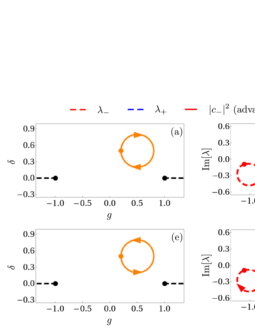
Figure 6: Closed trajectory not encircling an EP can lead to non-chiral state conversion. (a) and (e) — The clockwise and counterclockwise trajectories (orange) correspond to the following parameters in Eq. (9): $\delta_{0}=0.5$, $g_{0}=0.5$, $R=0.3$, $T=500$, $\omega=-2\pi/T$, $\phi=0$ (clockwise); $\delta_{0}=0.5$, $g_{0}=0.5$, $R=0.3$, $T=500$, $\omega=2\pi/T$, $\phi=0$ (counterclockwise). The trajectory direction is shown with arrows and the orange dot depict the starting point. The black dots correspond to the EPs of the Hamiltonian, and the dashed lines correspond to the branch cuts of $\lambda_{\pm}$. (b) and (f) — The trajectory of the eigenvalues $\lambda_{\pm}$ corresponding to the respective trajectory. The effect of perturbation $\varepsilon\delta H(t)$, cf. Eqs. (11–12) is clearly not noticeable here. The eigevalues $\lambda_{\pm}$ at the start of the parameter trajectory are depicted as blue and red dots, and the arrows show the trajectory direction. (c) and (g) — The population dynamics for the respective trajectory when the system is initialized in $\left|\psi_{-}\right\rangle$. (d) and (h) — The population dynamics for the respective trajectory encircling when the system is initialized in $\left|\psi_{+}\right\rangle$.

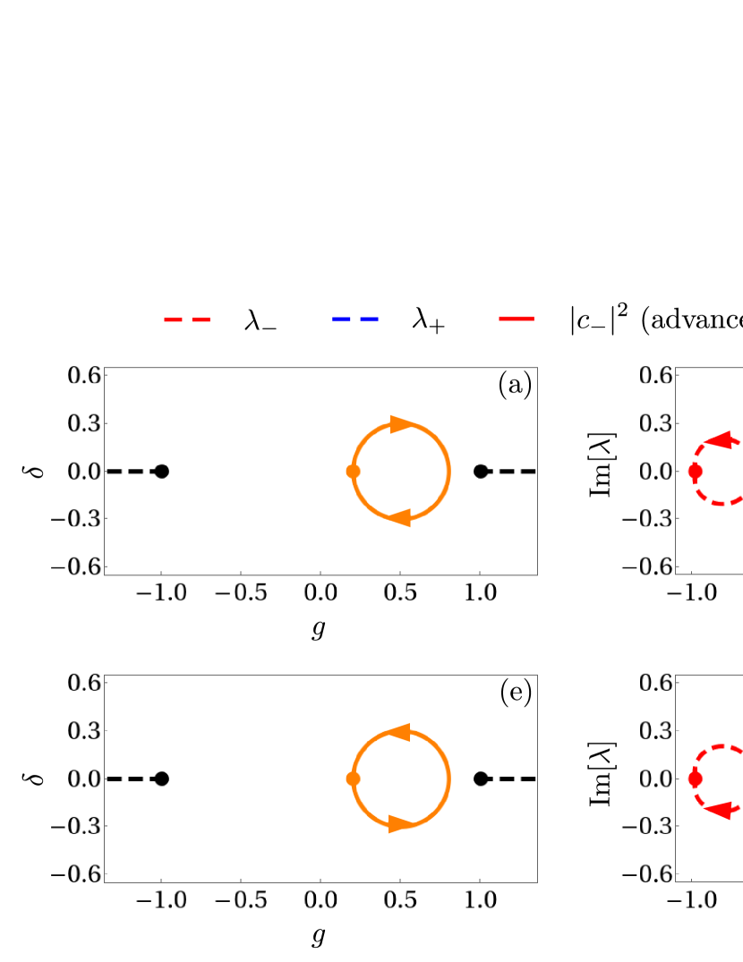
Figure 7: Closed trajectory not encircling an EP can lead to chiral state conversion. (a) and (e) — The clockwise and counterclockwise trajectories (orange) correspond to the following parameters in Eq. (9): $\delta_{0}=0$, $g_{0}=0.5$, $R=0.3$, $T=500$, $\omega=-2\pi/T$, $\phi=0$ (clockwise); $\delta_{0}=0$, $g_{0}=0.5$, $R=0.3$, $T=500$, $\omega=2\pi/T$, $\phi=0$ (counterclockwise). The trajectory direction is shown with arrows and the orange dot depict the starting point. The black dots correspond to the EPs of the Hamiltonian, and the dashed lines correspond to the branch cuts of $\lambda_{\pm}$. (b) and (f) — The trajectory of the eigenvalues $\lambda_{\pm}$ corresponding to the respective trajectory. The effect of perturbation $\varepsilon\delta H(t)$, cf. Eqs. (11–12) is clearly not noticeable here. The eigevalues $\lambda_{\pm}$ at the start of the parameter trajectory are depicted as blue and red dots, and the arrows show the trajectory direction. (c) and (g) — The population dynamics for the respective trajectory when the system is initialized in $\left|\psi_{-}\right\rangle$. (d) and (h) — The population dynamics for the respective trajectory encircling when the system is initialized in $\left|\psi_{+}\right\rangle$.

C.3 Closed evolution: with encircling the exceptional point

The evolution encircling an EP can similarly generate both non-chiral and chiral state conversion behaviors. The more conventional chiral conversion upon encircling an EP is shown in Fig. 8. Panels (c–d) and (g–h) show quantitative agreement between the numerical simulations and the predictions of the advanced theory.

The non-chiral conversion is exemplified in Fig. 9. The parameter trajectory is the same as in Sec. IV.2. Comparing the times of population switches between Figs. 9 and 3, one sees that, again, here the controlled perturbation $\varepsilon\delta H(t)$ (12) overshadows the perturbations due to numerical errors. Under these conditions, panels (c–d) and (g–h) show quantitative agreement between the numerical simulations and the predictions of the advanced theory. Note that the times of last population switch are not the same for the clockwise and the counterclockwise trajectories. This is because $\mathrm{Im}\,\lambda_{-}$ becomes larger than $\mathrm{Im}\,\lambda_{+}$ at different times depending on the trajectory direction. This further illustrates that it is the end-point fastest growing state that wins — the overall growth/decay over the early parts of the trajectory does not matter.

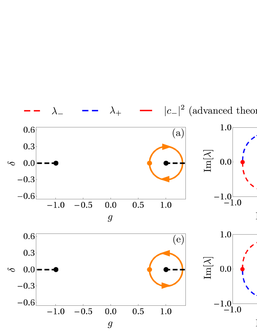
Figure 8: Closed trajectory encircling an EP can lead to chiral state conversion. (a) and (e) — The clockwise and counterclockwise trajectories (orange) correspond to the following parameters in Eq. (9): $\delta_{0}=0$, $g_{0}=1$, $R=0.3$, $T=500$, $\omega=-2\pi/T$, $\phi=0$ (clockwise), $\delta_{0}=0$, $g_{0}=1$, $R=0.3$, $T=500$, $\omega=2\pi/T$, $\phi=0$ (counterclockwise). The trajectory direction is shown with arrows and the orange dot depict the starting point. The black dots correspond to the EPs of the Hamiltonian, and the dashed lines correspond to the branch cuts of $\lambda_{\pm}$. (b) and (f) — The trajectory of the eigenvalues $\lambda_{\pm}$ corresponding to the respective trajectory. The effect of perturbation $\varepsilon\delta H(t)$, cf. Eqs. (11–12) is clearly not noticeable here. The eigevalues $\lambda_{\pm}$ at the start of the parameter trajectory are depicted as blue and red dots, and the arrows show the trajectory direction. (c) and (g) — The population dynamics for the respective trajectory when the system is initialized in $\left|\psi_{-}\right\rangle$. (d) and (h) — The population dynamics for the respective trajectory encircling when the system is initialized in $\left|\psi_{+}\right\rangle$.

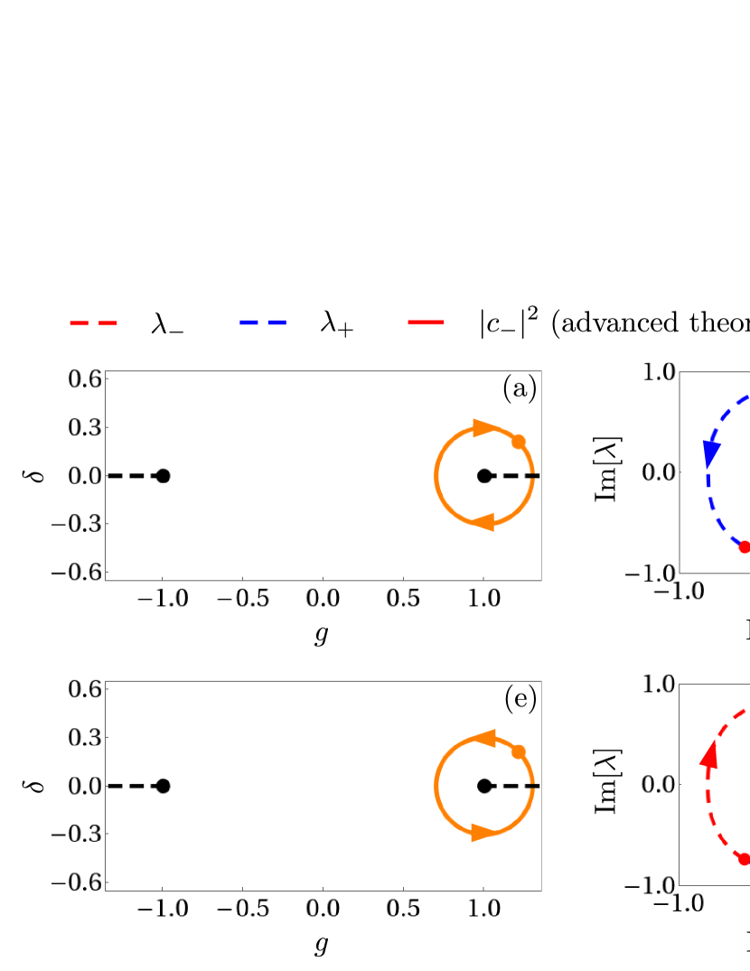
Figure 9: Closed trajectory encircling an EP can lead to non-chiral state conversion. (a) and (e) — The clockwise and counterclockwise trajectories (orange) correspond to the following parameters in Eq. (9): $\delta_{0}=0$, $g_{0}=1$, $R=0.3$, $T=500$, $\omega=-2\pi/T$, $\phi=-3\pi/4$ (clockwise), $\delta_{0}=0$, $g_{0}=1$, $R=0.3$, $T=500$, $\omega=2\pi/T$, $\phi=-3\pi/4$ (counterclockwise). The trajectory direction is shown with arrows and the orange dot depict the starting point. The black dots correspond to the EPs of the Hamiltonian, and the dashed lines correspond to the branch cuts of $\lambda_{\pm}$. (b) and (f) — The trajectory of the eigenvalues $\lambda_{\pm}$ corresponding to the respective trajectory. The effect of perturbation $\varepsilon\delta H(t)$, cf. Eqs. (11–12) is clearly not noticeable here. The eigevalues $\lambda_{\pm}$ at the start of the parameter trajectory are depicted as blue and red dots, and the arrows show the trajectory direction. (c) and (g) — The population dynamics for the respective trajectory when the system is initialized in $\left|\psi_{-}\right\rangle$. (d) and (h) — The population dynamics for the respective trajectory encircling when the system is initialized in $\left|\psi_{+}\right\rangle$.

References

- Bender [2007] C. M. Bender, Making sense of non-Hermitian Hamiltonians, Reports Prog. Phys. 70, 947 (2007).
- Bender [2019] C. M. Bender, PT Symmetry in Quantum and Classical Physics (World Scientific (Europe), 2019).
- Ashida et al. [2020] Y. Ashida, Z. Gong, and M. Ueda, Non-Hermitian physics, Adv. Phys. 69, 249 (2020), arXiv:2006.01837 .
- Bergholtz et al. [2021] E. J. Bergholtz, J. C. Budich, and F. K. Kunst, Exceptional topology of non-Hermitian systems, Rev. Mod. Phys. 93, 15005 (2021), arXiv:1912.10048 .
- Okuma and Sato [2023] N. Okuma and M. Sato, Non-Hermitian Topological Phenomena: A Review, Annu. Rev. Condens. Matter Phys. 14, 83 (2023).
- Banerjee et al. [2023] A. Banerjee, R. Sarkar, S. Dey, and A. Narayan, Non-Hermitian topological phases: principles and prospects, J. Phys. Condens. Matter 35, 10.1088/1361-648X/acd1cb (2023).
- Lévy and Williams [1982] L. P. Lévy and W. L. Williams, Role of Damping and Invariance in Induced Transitions in , Phys. Rev. Lett. 48, 1011 (1982).
- Naghiloo et al. [2019] M. Naghiloo, M. Abbasi, Y. N. Joglekar, and K. W. Murch, Quantum state tomography across the exceptional point in a single dissipative qubit, Nat. Phys. 15, 1232 (2019).
- Michishita and Peters [2020] Y. Michishita and R. Peters, Equivalence of Effective Non-Hermitian Hamiltonians in the Context of Open Quantum Systems and Strongly Correlated Electron Systems, Phys. Rev. Lett. 124, 196401 (2020), arXiv:2001.09045 .
- Abbasi et al. [2020] M. Abbasi, W. Chen, and K. W. Murch, Observing Non-Hermitian Evolution of a Single Dissipative Qubit Near an Exceptional Point, in Quantum 2.0 Conf. 2020 (2020) pp. 4–5.
- Chen et al. [2021] W. Chen, M. Abbasi, Y. N. Joglekar, and K. W. Murch, Quantum Jumps in the Non-Hermitian Dynamics of a Superconducting Qubit, Phys. Rev. Lett. 127, 140504 (2021), arXiv:2103.06274 .
- Chen et al. [2022a] W. Chen, M. Abbasi, B. Ha, S. Erdamar, Y. N. Joglekar, and K. W. Murch, Decoherence-Induced Exceptional Points in a Dissipative Superconducting Qubit, Phys. Rev. Lett. 128, 110402 (2022a), arXiv:2111.04754 .
- Li et al. [2023] Z.-Z. Li, W. Chen, M. Abbasi, K. W. Murch, and K. B. Whaley, Speeding Up Entanglement Generation by Proximity to Higher-Order Exceptional Points, Phys. Rev. Lett. 131, 100202 (2023).
- Ohnmacht et al. [2024] D. C. Ohnmacht, V. Wilhelm, H. Weisbrich, and W. Belzig, Non-hermitian topology in multiterminal superconducting junctions, arXiv:2408.01289 (2024).
- Huang et al. [2019] M. Huang, R.-K. Lee, L. Zhang, S.-M. Fei, and J. Wu, Simulating Broken -Symmetric Hamiltonian Systems by Weak Measurement, Phys. Rev. Lett. 123, 080404 (2019).
- Snizhko et al. [2020] K. Snizhko, P. Kumar, and A. Romito, Quantum Zeno effect appears in stages, Phys. Rev. Res. 2, 033512 (2020), arXiv:2003.10476 .
- Chenu et al. [2017] A. Chenu, M. Beau, J. Cao, and A. del Campo, Quantum Simulation of Generic Many-Body Open System Dynamics Using Classical Noise, Phys. Rev. Lett. 118, 140403 (2017), arXiv:1608.01317 .
- Dupays et al. [2020] L. Dupays, I. L. Egusquiza, A. del Campo, and A. Chenu, Superadiabatic thermalization of a quantum oscillator by engineered dephasing, Phys. Rev. Res. 2, 033178 (2020), arXiv:1910.12088 .
- Dupays and Chenu [2021] L. Dupays and A. Chenu, Shortcuts to Squeezed Thermal States, Quantum 5, 449 (2021), arXiv:1810.13295 .
- Martinez-Azcona et al. [2023] P. Martinez-Azcona, A. Kundu, A. del Campo, and A. Chenu, Stochastic Operator Variance: An Observable to Diagnose Noise and Scrambling, Phys. Rev. Lett. 131, 160202 (2023), arXiv:2302.12845 .
- Martinez-Azcona et al. [2024] P. Martinez-Azcona, A. Kundu, A. Saxena, A. del Campo, and A. Chenu, Quantum Dynamics with Stochastic Non-Hermitian Hamiltonians, arXiv:2407.07746 (2024).
- Avron et al. [2011] J. E. Avron, M. Fraas, G. M. Graf, and P. Grech, Landau-Zener Tunneling for Dephasing Lindblad Evolutions, Commun. Math. Phys. 305, 633 (2011), arXiv:0912.4640 .
- Albert et al. [2016] V. V. Albert, B. Bradlyn, M. Fraas, and L. Jiang, Geometry and Response of Lindbladians, Phys. Rev. X 6, 041031 (2016), arXiv:1512.08079 .
- Fraas and Hänggli [2017] M. Fraas and L. Hänggli, On Landau–Zener Transitions for Dephasing Lindbladians, Ann. Henri Poincaré 18, 2447 (2017).
- Minganti et al. [2019] F. Minganti, A. Miranowicz, R. W. Chhajlany, and F. Nori, Quantum exceptional points of non-Hermitian Hamiltonians and Liouvillians: The effects of quantum jumps, Phys. Rev. A 100, 062131 (2019), arXiv:1909.11619 .
- Pick et al. [2019] A. Pick, S. Silberstein, N. Moiseyev, and N. Bar-Gill, Robust mode conversion in NV centers using exceptional points, Phys. Rev. Res. 1, 013015 (2019), arXiv:1905.00759 .
- Lieu et al. [2020] S. Lieu, M. McGinley, and N. R. Cooper, Tenfold Way for Quadratic Lindbladians, Phys. Rev. Lett. 124, 040401 (2020), arXiv:1908.08834 .
- Kumar et al. [2021] P. Kumar, K. Snizhko, and Y. Gefen, Near-unit efficiency of chiral state conversion via hybrid-Liouvillian dynamics, Phys. Rev. A 104, L050405 (2021), arXiv:2105.02251 .
- Kumar et al. [2022] P. Kumar, K. Snizhko, Y. Gefen, and B. Rosenow, Optimized steering: Quantum state engineering and exceptional points, Phys. Rev. A 105, L010203 (2022).
- Joye [2022] A. Joye, Adiabatic Lindbladian Evolution with Small Dissipators, Commun. Math. Phys. 391, 223 (2022), arXiv:2106.15749 .
- Bu et al. [2023] J.-T. Bu, J.-Q. Zhang, G.-Y. Ding, J.-C. Li, J.-W. Zhang, B. Wang, W.-Q. Ding, W.-F. Yuan, L. Chen, S. K. Özdemir, F. Zhou, H. Jing, and M. Feng, Enhancement of Quantum Heat Engine by Encircling a Liouvillian Exceptional Point, Phys. Rev. Lett. 130, 110402 (2023), arXiv:2302.13450 .
- Zhou et al. [2023] Y.-L. Zhou, X.-D. Yu, C.-W. Wu, X.-Q. Li, J. Zhang, W. Li, and P.-X. Chen, Accelerating relaxation through Liouvillian exceptional point, Phys. Rev. Res. 5, 043036 (2023), arXiv:2305.12745 .
- Larson and Qvarfort [2023] J. Larson and S. Qvarfort, Exceptional Points and Exponential Sensitivity for Periodically Driven Lindblad Equations, Open Syst. Inf. Dyn. 30, 2350008 (2023), arXiv:2306.12322 .
- Pavlov et al. [2024] A. I. Pavlov, Y. Gefen, and A. Shnirman, Topological transitions in quantum jump dynamics: Hidden exceptional points, arXiv:2408.05270 (2024).
- Gao et al. [2025] H. Gao, K. Sun, D. Qu, K. Wang, L. Xiao, W. Yi, and P. Xue, Photonic chiral state transfer near the Liouvillian exceptional point, arXiv:2501.10349 (2025).
- Okuma et al. [2020] N. Okuma, K. Kawabata, K. Shiozaki, and M. Sato, Topological Origin of Non-Hermitian Skin Effects, Phys. Rev. Lett. 124, 86801 (2020), arXiv:1910.02878 .
- Kawabata et al. [2019] K. Kawabata, K. Shiozaki, M. Ueda, and M. Sato, Symmetry and Topology in Non-Hermitian Physics, Phys. Rev. X 9, 041015 (2019), arXiv:1812.09133 .
- McDonald and Clerk [2020] A. McDonald and A. A. Clerk, Exponentially-enhanced quantum sensing with non-Hermitian lattice dynamics, Nat. Commun. 11, 5382 (2020), arXiv:2004.00585 .
- Li et al. [2021] T. Li, Y.-S. Zhang, and W. Yi, Two-Dimensional Quantum Walk with Non-Hermitian Skin Effects, Chinese Phys. Lett. 38, 030301 (2021), arXiv:2005.09474 .
- Spring et al. [2023] H. Spring, V. Könye, A. R. Akhmerov, and I. C. Fulga, Lack of near-sightedness principle in non-Hermitian systems, arXiv:2308.00776 (2023).
- Matsumoto et al. [2020] N. Matsumoto, K. Kawabata, Y. Ashida, S. Furukawa, and M. Ueda, Continuous Phase Transition without Gap Closing in Non-Hermitian Quantum Many-Body Systems, Phys. Rev. Lett. 125, 260601 (2020), arXiv:1912.09045 .
- Kawabata et al. [2020] K. Kawabata, N. Okuma, and M. Sato, Non-Bloch band theory of non-Hermitian Hamiltonians in the symplectic class, Phys. Rev. B 101, 195147 (2020), arXiv:2003.07597 .
- Wiersig [2020] J. Wiersig, Prospects and fundamental limits in exceptional point-based sensing, Nat. Commun. 11, 2454 (2020).
- Teixeira et al. [2023] W. S. Teixeira, V. Vadimov, T. Mörstedt, S. Kundu, and M. Möttönen, Exceptional-point-assisted entanglement, squeezing, and reset in a chain of three superconducting resonators, Phys. Rev. Res. 5, 033119 (2023).
- Li et al. [2022] A. Li, W. Chen, H. Wei, G. Lu, A. Alù, C.-w. Qiu, and L. Chen, Riemann-Encircling Exceptional Points for Efficient Asymmetric Polarization-Locked Devices, Phys. Rev. Lett. 129, 127401 (2022).
- Arkhipov et al. [2023] I. I. Arkhipov, A. Miranowicz, F. Minganti, S. K. Özdemir, and F. Nori, Dynamically crossing diabolic points while encircling exceptional curves: A programmable symmetric-asymmetric multimode switch, Nat. Commun. 14, 2076 (2023).
- Arkhipov et al. [2025] I. I. Arkhipov, P. Lewalle, F. Nori, S. K. Özdemir, and K. B. Whaley, State Permutation Control in Non-Hermitian Multiqubit Systems with Suppressed Non-Adiabatic Transitions, arXiv:2501.16160 (2025).
- Chen et al. [2022b] Y.-Q. Chen, S.-X. Zhang, C.-Y. Hsieh, and S. Zhang, A non-Hermitian Ground State Searching Algorithm Enhanced by Variational Toolbox, arXiv:2210.09007 (2022b).
- Uzdin et al. [2011] R. Uzdin, A. Mailybaev, and N. Moiseyev, On the observability and asymmetry of adiabatic state flips generated by exceptional points, J. Phys. A Math. Theor. 44, 435302 (2011).
- Berry and Uzdin [2011] M. V. Berry and R. Uzdin, Slow non-Hermitian cycling: exact solutions and the Stokes phenomenon, J. Phys. A Math. Theor. 44, 435303 (2011).
- Gilary et al. [2013] I. Gilary, A. A. Mailybaev, and N. Moiseyev, Time-asymmetric quantum-state-exchange mechanism, Phys. Rev. A 88, 010102 (2013).
- Graefe et al. [2013] E.-M. Graefe, A. A. Mailybaev, and N. Moiseyev, Breakdown of adiabatic transfer of light in waveguides in the presence of absorption, Phys. Rev. A 88, 033842 (2013), arXiv:1207.5235 .
- Milburn et al. [2015] T. J. Milburn, J. Doppler, C. A. Holmes, S. Portolan, S. Rotter, and P. Rabl, General description of quasiadiabatic dynamical phenomena near exceptional points, Phys. Rev. A 92, 052124 (2015), arXiv:1410.1882 .
- Doppler et al. [2016] J. Doppler, A. A. Mailybaev, J. Böhm, U. Kuhl, A. Girschik, F. Libisch, T. J. Milburn, P. Rabl, N. Moiseyev, and S. Rotter, Dynamically encircling an exceptional point for asymmetric mode switching, Nature 537, 76 (2016).
- Hassan et al. [2017a] A. U. Hassan, B. Zhen, M. Soljačić, M. Khajavikhan, and D. N. Christodoulides, Dynamically Encircling Exceptional Points: Exact Evolution and Polarization State Conversion, Phys. Rev. Lett. 118, 093002 (2017a), arXiv:1706.09938 .
- Hassan et al. [2017b] A. U. Hassan, G. L. Galmiche, G. Harari, P. LiKamWa, M. Khajavikhan, M. Segev, and D. N. Christodoulides, Chiral state conversion without encircling an exceptional point, Phys. Rev. A 96, 052129 (2017b).
- Hassan et al. [2017c] A. U. Hassan, G. L. Galmiche, G. Harari, P. LiKamWa, M. Khajavikhan, M. Segev, and D. N. Christodoulides, Erratum: Chiral state conversion without encircling an exceptional point [Phys. Rev. A 96 , 052129 (2017)], Phys. Rev. A 96, 069908 (2017c).
- Zhong et al. [2018] Q. Zhong, M. Khajavikhan, D. N. Christodoulides, and R. El-Ganainy, Winding around non-Hermitian singularities, Nat. Commun. 9, 4808 (2018).
- Zhang et al. [2018] X.-L. Zhang, S. Wang, B. Hou, and C. T. Chan, Dynamically Encircling Exceptional Points: In situ Control of Encircling Loops and the Role of the Starting Point, Phys. Rev. X 8, 021066 (2018), arXiv:1804.09145 .
- Zhang et al. [2019] X.-L. Zhang, J.-F. Song, C. T. Chan, and H.-B. Sun, Distinct outcomes by dynamically encircling an exceptional point along homotopic loops, Phys. Rev. A 99, 063831 (2019).
- Feilhauer et al. [2020] J. Feilhauer, A. Schumer, J. Doppler, A. A. Mailybaev, J. Böhm, U. Kuhl, N. Moiseyev, and S. Rotter, Encircling exceptional points as a non-Hermitian extension of rapid adiabatic passage, Phys. Rev. A 102, 040201 (2020), arXiv:2004.05486 .
- Li et al. [2020] A. Li, J. Dong, J. Wang, Z. Cheng, J. S. Ho, D. Zhang, J. Wen, X.-l. Zhang, C. T. Chan, A. Alù, C.-w. Qiu, and L. Chen, Hamiltonian Hopping for Efficient Chiral Mode Switching in Encircling Exceptional Points, Phys. Rev. Lett. 125, 187403 (2020).
- Choi et al. [2020] Y. Choi, J. W. Yoon, J. K. Hong, Y. Ryu, and S. H. Song, Direct observation of time-asymmetric breakdown of the standard adiabaticity around an exceptional point, Commun. Phys. 3, 140 (2020).
- Ribeiro and Marquardt [2021] H. Ribeiro and F. Marquardt, Accelerated Non-Reciprocal Transfer of Energy Around an Exceptional Point, arXiv:2111.11220 (2021).
- Laha et al. [2021] A. Laha, D. Beniwal, and S. Ghosh, Successive switching among four states in a gain-loss-assisted optical microcavity hosting exceptional points up to order four, Phys. Rev. A 103, 023526 (2021).
- Liu et al. [2021] W. Liu, Y. Wu, C.-K. Duan, X. Rong, and J. Du, Dynamically Encircling an Exceptional Point in a Real Quantum System, Phys. Rev. Lett. 126, 170506 (2021), arXiv:2002.06798 .
- Sun and Yi [2023] K. Sun and W. Yi, Chiral state transfer under dephasing, Phys. Rev. A 108, 013302 (2023).
- Nasari et al. [2022] H. Nasari, G. Lopez-Galmiche, H. E. Lopez-Aviles, A. Schumer, A. U. Hassan, Q. Zhong, S. Rotter, P. LiKamWa, D. N. Christodoulides, and M. Khajavikhan, Observation of chiral state transfer without encircling an exceptional point, Nature 605, 256 (2022).
- Guria et al. [2024] C. Guria, Q. Zhong, S. K. Ozdemir, Y. S. S. Patil, R. El-Ganainy, and J. G. E. Harris, Resolving the topology of encircling multiple exceptional points, Nat. Commun. 15, 1369 (2024).
- Fan et al. [2023] Z. Fan, D. Long, X. Mao, G.-Q. Qin, M. Wang, G.-Q. Li, and G.-L. Long, Proximity-encirclement of exceptional points in a multimode optomechanical system, arXiv:2305.15682 (2023).
- Zhang et al. [2023] Y. Zhang, W. Liu, S. Ren, T. Chai, Y. Wang, H. Long, K. Wang, B. Wang, and P. Lu, Asymmetric Switching of Edge Modes by Dynamically Encircling Multiple Exceptional Points, Phys. Rev. Appl. 19, 064050 (2023).
- Qi et al. [2024] H. Qi, Y. Li, X. Wang, Y. Li, X. Li, X. Wang, X. Hu, and Q. Gong, Dynamically Encircling Exceptional Points in Different Riemann Sheets for Orbital Angular Momentum Topological Charge Conversion, Phys. Rev. Lett. 132, 243802 (2024).
- Shan et al. [2024] Z.-l. Shan, Y.-k. Sun, R. Tao, Q.-d. Chen, Z.-n. Tian, and X.-l. Zhang, Non-Abelian Holonomy in Degenerate Non-Hermitian Systems, Phys. Rev. Lett. 133, 053802 (2024).
- Alizadeh and Amirkhizi [2024] V. Alizadeh and A. V. Amirkhizi, In-Plane Stress Waves in Layered Media: I. Non-Hermitian Degeneracies and Modal Chirality, arXiv:2409.16162 (2024).
- Zhang et al. [2024] H. Zhang, T. Liu, Z. Xiang, K. Xu, H. Fan, and D. Zheng, Topological eigenvalues braiding and quantum state transfer near a third-order exceptional point, arXiv:2412.14733 (2024).
- Ho et al. [2024] K. Ho, S. Perna, S. Wittrock, S. Tsunegi, H. Kubota, S. Yuasa, P. Bortolotti, M. D’Aquino, C. Serpico, V. Cros, and R. Lebrun, Controlling encirclement of an exceptional point using coupled spintronic nano-oscillators, arXiv:2412.17037 (2024).
- Chavva and Ribeiro [2025] V. Chavva and H. Ribeiro, Topological Operations Around Exceptional Points via Shortcuts to Adiabaticity, arXiv:2501.07454 (2025).
- Nye [2023] N. S. Nye, Universal state conversion in discrete and slowly varying non-Hermitian cyclic systems: An analytic proof and exactly solvable examples, Phys. Rev. Res. 5, 10.1103/PhysRevResearch.5.033053 (2023).
- Nye and Kantartzis [2024] N. S. Nye and N. V. Kantartzis, Adiabatic state conversion for (a)cyclic non-Hermitian quantum Hamiltonians of generalized functional form, APL Quantum 1, 10.1063/5.0225403 (2024).
- Kvitsinsky and Putterman [1991] A. Kvitsinsky and S. Putterman, Adiabatic evolution of an irreversible two level system, J. Math. Phys. 32, 1403 (1991).
- Nenciu and Rasche [1992] G. Nenciu and G. Rasche, On the adiabatic theorem for nonself-adjoint Hamiltonians, J. Phys. A. Math. Gen. 25, 5741 (1992).
- Avron et al. [2012] J. E. Avron, M. Fraas, G. M. Graf, and P. Grech, Adiabatic Theorems for Generators of Contracting Evolutions, Commun. Math. Phys. 314, 163 (2012), arXiv:1106.4661 .
- Hwang and Pechukas [1977] J.-T. Hwang and P. Pechukas, The adiabatic theorem in the complex plane and the semiclassical calculation of nonadiabatic transition amplitudes, J. Chem. Phys. 67, 4640 (1977).
- Joye and Pfister [1991] A. Joye and C. E. Pfister, Full asymptotic expansion of transition probabilities in the adiabatic limit, J. Phys. A. Math. Gen. 24, 753 (1991).
- Joye et al. [1991] A. Joye, H. Kunz, and C.-E. Pfister, Exponential decay and geometric aspect of transition probabilities in the adiabatic limit, Ann. Phys. (N. Y). 208, 299 (1991).
- Joye [1997] A. Joye, Exponential Asymptotics in a Singular Limit for n-Level Scattering Systems, SIAM J. Math. Anal. 28, 669 (1997).
- Joye [2007] A. Joye, General Adiabatic Evolution with a Gap Condition, Commun. Math. Phys. 275, 139 (2007).
- [88] https://github.com/KyryloSnizhko/SlowNonHermitianEvolution.
- Longhi and Feng [2023] S. Longhi and L. Feng, Complex Berry phase and imperfect non-Hermitian phase transitions, Phys. Rev. B 107, 085122 (2023).
- Zener [1932] C. Zener, Non-adiabatic crossing of energy levels, Proc. R. Soc. London. Ser. A, Contain. Pap. a Math. Phys. Character 137, 696 (1932).
- Landau [1932] L. D. Landau, On the theory of transfer of energy at collisions II, Phys. Z. Sowjetunion 2, 46 (1932).
- Stueckelberg [1932] E. C. G. Stueckelberg, Theorie der unelastischen Stösse zwischen Atomen, Helv. Phys. Acta 5, 369 (1932).
- Majorana [1932] E. Majorana, Atomi orientati in campo magnetico variabile, Nuovo Cim. 9, 43 (1932).
- Landau and Lifshitz [1977] L. D. Landau and E. M. Lifshitz, Pre-dissociation, in Quantum Mech. Non-relativistic Theory (Pergamon, New York, 1977) 3rd ed., pp. 342–351.
- Rubbmark et al. [1981] J. R. Rubbmark, M. M. Kash, M. G. Littman, and D. Kleppner, Dynamical effects at avoided level crossings: A study of the Landau-Zener effect using Rydberg atoms, Phys. Rev. A 23, 3107 (1981).
- Mullen et al. [1989] K. Mullen, E. Ben-Jacob, Y. Gefen, and Z. Schuss, Time of Zener tunneling, Phys. Rev. Lett. 62, 2543 (1989).
- Lubin et al. [1990] D. Lubin, Y. Gefen, and I. Goldhirsch, Zener dynamics beyond Zener’s assumptions, Phys. A Stat. Mech. its Appl. 168, 456 (1990).
- Shimshoni and Gefen [1991] E. Shimshoni and Y. Gefen, Onset of dissipation in Zener dynamics: Relaxation versus dephasing, Ann. Phys. (N. Y). 210, 16 (1991).
- Shimshoni and Stern [1993] E. Shimshoni and A. Stern, Dephasing of interference in Landau-Zener transitions, Phys. Rev. B 47, 9523 (1993).
- Malla et al. [2023] R. K. Malla, J. Cen, W. J. M. Kort-Kamp, and A. Saxena, Quantum dynamics of non-Hermitian many-body Landau-Zener systems, arXiv:2304.03471 (2023).