Path Planning for Masked Diffusion Model Sampling

Abstract

In this paper, we explore how token unmasking order influences generative quality in masked diffusion models (MDMs). We derive an expanded evidence lower bound (ELBO) that introduces a planner to select which tokens to unmask at each step. Our analysis reveals that alternative unmasking strategies can enhance generation performance. Building on this, we propose Path Planning (P2), a sampling framework that uses a pre-trained BERT model or the denoiser itself to guide unmasking decisions. P2 generalizes all known MDM sampling strategies and significantly improves performance across diverse domains, including language generation (in-context learning, code generation, story infilling, mathematical reasoning, reverse curse correction) and biological sequence generation (protein and RNA sequences).

1 Introduction

Inspired by the success of diffusion models in continuous space and the desire for bidirectional reasoning, much work has sought to design performant training algorithms for discrete diffusion models. While there are many possible discrete noising processes, most successful discrete diffusion approaches have converged to absorbing state diffusion (Austin et al., 2021; Lou et al., 2023) with new, simplified training objectives resulting in scalable masked diffusion models (MDMs) (Sahoo et al., 2024; Shi et al., 2024; Gat et al., 2024).

While most recent work has focused on improving MDM training, considerably less attention has been given to the impact of inference techniques on overall generative performance. This raises a question: Can we design new inference strategies to improve generative quality? In this paper, we answer affirmatively by investigating how the order in which tokens are unmasked during MDM inference affects generative quality. While the MDM reverse process requires that each token is uniformly likely to be unmasked at a given step, this correctly reconstructs the true data distribution only under a perfect denoiser (for further discussion of this perspective, see Appendix D.1). However, since any trained MDM is inherently imperfect and does not yield a tight ELBO, it has been empirically observed that a uniformly random unmasking order is suboptimal in many settings (Ou et al., 2024; Shih et al., 2022; Li et al., 2021).

We begin our study by reexamining the typical MDM ELBO and show that, for a fixed denoiser, we can expand the ELBO to include two additional terms, both involving a “planner” whose role is to select which tokens should be unmasked at a given inference step as well as optionally choosing already unmasked tokens to be remasked. Our ELBO shows that while the optimal planner for the optimal denoiser is indeed uniform unmasking, the strategy prescribed by the reverse process, one can obtain better generative quality for an imperfect denoiser through the use of a well tuned, non-uniform planner. Of particular note is that the ELBO’s planner terms are effectively a reweighting of the typical MLM objective with additional small differences due to an added dependence on the denoiser.

These observations lead to our proposed method, Path Planning (P2), which makes use of the expanded ELBO to introduce a family of planners for use at inference time. Crucially, by noting the similarity between the planner ELBO terms and the typical MLM objective we show that in practice we can obtain effective planners fully training-free by employing either pre-trained BERT-type models or simply using the already trained denoiser. Moreover, P2 is shown the generalize all known existing sampling strategies in the MDM literature (see Table 1). We validate our training-free planning framework across a diverse set of experimental settings, showing that by using P2 a 1B parameter MDM model can outperform a 7B Llama model in math reasoning while far outpacing state-of-the-art ARMs for code generation on same same-sized models. At the same time, for biological sequence design we show that the combination of P2 and DPLM (Wang et al., 2024a) leads to state-of-the-art generation quality for proteins, while for RNA design we outperform competitive models and observe that our sequences lead to higher structural plausibility than even true, naturally occurring sequences.

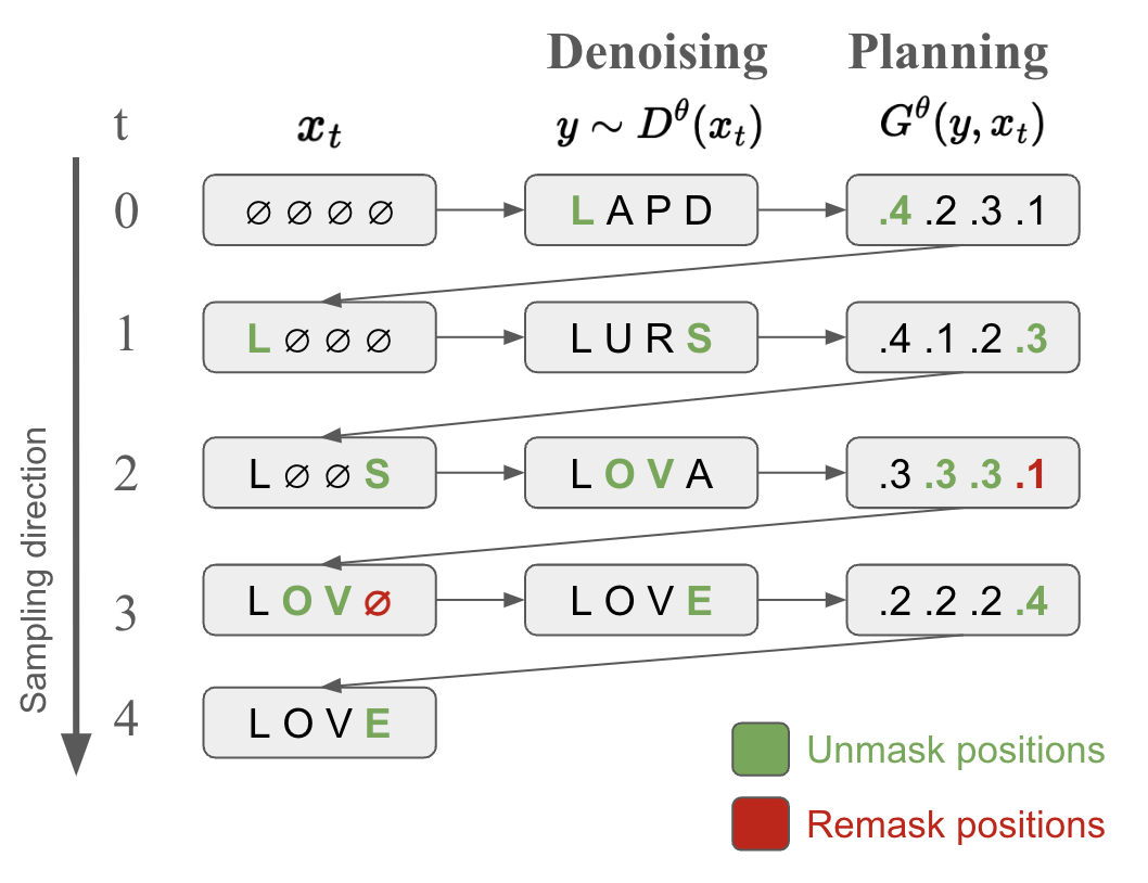
Figure 1: An example of the P2 sampling strategy (see Algorithm 1). In each step, the denoiser $D^{\theta}(\cdot)$ makes predictions and the planner $G^{\theta}(\cdot)$ ranks and selects positions to unmask (green colored) and remask (red colored).

2 Background

Notation

We will denote by $S=\{1,\ldots,N\}$ a finite dictionary of tokens, by $\bar{S}=S\cup\{M\}$ the extension of this dictionary via the addition of some masked state $M$. For a metric space $\mathcal{X}$, we define by $\mathcal{P}(\mathcal{X})$ the space of Borel probability measures on $\mathcal{X}$. When $\mathcal{X}$ is finite we endow $\mathcal{X}$ with the discrete metric and let $|\mathcal{X}|$ denote the cardinality of $\mathcal{X}$. With some abuse of notation we freely identify $\mu\in\mathcal{P}(\mathcal{X})$ with a column vector in $[0,1]^{|X|}$ corresponding to the associated probability mass function. We denote by $\delta_{x}\in\mathcal{P}(\mathcal{X})$ the probability measure such that $\delta_{x}(y)\coloneqq 1$ if $x=y$ and $0$ otherwise and by $\text{Unif}(\mathcal{X})\in\mathcal{P}(\mathcal{X})$ the uniform probability measure on $\mathcal{X}$. We suppose that we are interested in generating sequences of length $L$ comprised of elements of $S$ from some data distribution $p_{\text{data}}\in\mathcal{P}(S^{L})$. We use $x_{i}$ to denote the $i$’th coordinate of an elements $x\in\bar{S}^{L}$, and $x^{-i}$ to denote the element in $\bar{S}^{L-1}$ which is the same as $x$ but with the $i$’th token removed. For $x\in\bar{S}^{L}$ and $y\in\bar{S}$, we denote by $x^{-i,y}$ the element in $\bar{S}^{L}$ which is the same as $x$ but with the $i$’th token replaced by $y$. We denote by $M^{L}\coloneqq(M,\dots,M)\in\bar{S}^{L}$.

2.1 Masked Diffusion Models

In a masked diffusion model, one starts with a a collection of probability mass functions given by, for $y\in\bar{S}^{L}$ and $t\in[0,1]$:

$$P_{t}(y;p_{\text{data}})\coloneqq\alpha(t)p_{\text{data}}(y)+(1-\alpha(t))\delta_{M^{L}}(y)$$ (1)

for a monotone-decreasing, continuously differentiable noise scheduler $\alpha:[0,1]\rightarrow[0,1]$ with $\alpha(0)=1$ and $\alpha(1)=0$, and finds continuous time Markov chain $\overset{\leftarrow}{X}_{t}$ such that $\mathbb{P}(X_{t}=x)=P_{1-t}(x;p_{\text{data}})$.

A rate matrix generating $\overset{\leftarrow}{X}_{t}$ is given for $x\neq y\in\bar{S}^{L}$, by:

$$\overset{\leftarrow}{Q}(y,x)=-\frac{\dot{\alpha}(1-t)}{1-\alpha(1-t)}\sum_{i=1}^{L}\delta_{M}(x_{i})p^{i}_{data}(y_{i}|x_{\neq M})\delta_{y^{-i}}(x^{-i})$$

and $\overset{\leftarrow}{Q}(x,x)=\frac{\dot{\alpha}(1-t)}{1-\alpha(1-t)}\sum_{i=1}^{L}\delta_{M}(x_{i})$ (see e.g. (Ou et al., 2024) Theorem 1). Here for $z\in\bar{S}^{L}$, $z_{\neq M}$ denotes the coordinates of $z$ which are not equal to $M$, and for $i\in\{1,\ldots,L\}$, and $j\in S$:

$$p^{i}_{data}(j|z_{\neq M})\coloneqq p_{data}(\{x:x_{i}=j\}|z_{\neq M}).$$

One then attempts to approximate $\overset{\leftarrow}{X}_{t}$ with $X^{\theta,\text{mask}}_{t}$ with transition matrix given for $x\neq y$ by:

$$Q^{\theta,\text{mask}}_{t}(y,x) \coloneqq-\frac{\dot{\alpha}(1-t)}{1-\alpha(1-t)}\sum_{i=1}^{L}\delta_{M}(x_{i})D_{i,y_{i}}^{\theta}(x)\delta_{y^{-i}}(x^{-i}).$$ (2)

Here we are using the “mean parametrization” of the approximate backwards matrix. That is, we have a neural network parameterized by $\theta$ which gives a “denoising function” $D^{\theta}:\bar{S}^{L}\rightarrow\mathcal{P}(S)^{L}$, with the hope that

$$D_{i,\cdot}^{\theta}(x)\approx p^{i}_{data}(\cdot|x_{\neq M})\in\mathcal{P}(S).$$ (3)

In particular, one enforces during inference that $D^{\theta}_{i,y_{i}}(x)=\delta_{x_{i}}(y_{i})$ if $x_{i}\neq M$.

Approximate samples from the data distribution are then obtained via simulating the Markov chain $X^{\theta,\text{mask}}$ with $X^{\theta,\text{mask}}_{0}=M^{L}$ to time 1.

3 Path Planning

Table 1: Generalization of Existing Sampling Methods within Our P2 Framework. Mask Planner ($G^{M}_{j}(y,x)$) gives the likelihood that a mask token should be unmasked. Unmask Planner ($G^{U}_{j}(y,x)$) gives the likelihood that an unmask token should be kept. $D^{\theta}_{j,y_{j}}(x)$ gives the prediction probability of the denoiser at position j for token $y_{j}$. $B^{\theta}(\cdot)$ is a BERT. $G^{\theta}(\cdot)$ is an external planner.

Method	Remasking	Planning	Stochasticity Control	Mask Planner ($G^{M}_{j}(y,x)$)	Unmask Planner ($G^{U}_{j}(y,x)$)
Ancestral (Shi et al., 2024; Sahoo et al., 2024)	✗	✗	✗	$\mathcal{U}(0,1)$	1
Greedy Ancestral (Gong et al., 2024)	✗	✓	✗	$D^{\theta}_{j,y_{j}}(x)$	1
DFM Sampling (Campbell et al., 2024)	✗	✗	✓	$\mathcal{U}(0,1)$	$\mathcal{U}(0,1)$
RDM Sampling (Zheng et al., 2023; Wang et al., 2024a, b)	✓	✓	✗	$D^{\theta}_{j,y_{j}}(x)$	$D^{\theta}_{j,y_{j}}(x)$
DDPD (Liu et al., 2024)	✓	✓	✗	$G^{\theta}_{j}(y)$	$G^{\theta}_{j}(y)$
Path Planning (Self-Planning, ours)	✓	✓	✓	$D^{\theta}_{j,y_{j}}(x)$	$D^{\theta}_{j,y_{j}}(x)$
Path Planning (BERT Planner, ours)	✓	✓	✓	$D^{\theta}_{j,y_{j}}(x)$	$B^{\theta}_{j,y_{j}}(y)$

3.1 Mathematical Formulation

In order to formulate P2 we begin by modifying the jump matrix for the approximate backwards process (Eq. 2), introducing a new function $G^{\theta}:S^{L}\times\bar{S}^{L}\rightarrow[0,1]^{L}$, which we refer to as the planner. $G_{j}^{\theta}(y,x)$ approximates the likelihood that the $j$’th token in a partially denoised sequence $x\in\bar{S}^{L}$ should be (re)sampled given the conditional information about the rest of the sequence $x$ and of the clean data $y$ as predicted by $D^{\theta}$. In Section 3.3, we discuss potential choices of planners and how previous works fall into this general framework.

We next define $F^{\theta}:\bar{S}^{L}\times\bar{S}^{L}\rightarrow[0,1]^{L}$ by

$$F^{\theta}_{j}(y,x) \coloneqq\delta_{M}(x_{j})\mathbb{E}_{Y\sim D^{\theta}(x)}[G^{\theta}_{j}(Y^{-j,y_{j}},x)]$$

$$+(1-\delta_{M}(x_{j}))\mathbb{E}_{Y\sim D^{\theta}(x)}[G^{\theta}_{j}(Y^{-j,x_{j}},x)]$$

where here we use the shorthand $Y\sim D^{\theta}(x)$ to mean $Y\sim\otimes_{i=1}^{L}D^{\theta}_{i,\cdot}(x)$.

Via our interpretation of the role of $G^{\theta}$, $F_{j}^{\theta}(y,x)$ gives the likelihood that the $j$’th position of $x$ should be (re)sampled given the information about the rest of the sequence $x$ and the data’s $j$’th token via averaging out the information provided about the rest of the data’s tokens from $D^{\theta}$.

Finally, we define

$$\hat{D}^{\theta}_{i,y_{i}}(x)=D^{\theta}_{i,y_{i}}(x)\delta_{M}(x_{i})+\frac{D^{\theta}_{i,y_{i}}(x^{-i,M})}{1-D^{\theta}_{i,x_{i}}(x^{-i,M})}(1-\delta_{M}(x_{i})).$$

That is, when $x_{i}$ is masked $\hat{D}^{\theta}_{i,y_{i}}(x)$ approximates the probability that the $i$’th token of $x$ should be unmasked to $y_{i}$ given the conditional information about the unmasked tokens in $x$, and when $x^{i}$ is not masked, $\hat{D}^{\theta}_{i,y_{i}}(x)$ approximates the probability that $i$’th token of $x$ should be resampled to a value other than $x_{i}$, given the conditional information about the unmasked tokens in $x$ other than $x_{i}$.

We now seek to modify $Q^{\theta,\text{mask}}$ from Eq. 2 in a way so that $F^{\theta}$ - by way of the planner $G^{\theta}$ - plays the role of selecting which position should be unmasked/resampled and $\hat{D}^{\theta}$ plays the role of choosing what it should be (re)sampled to.

For $x\neq y\in\bar{S}^{L}$, we thus set:

$$Q^{\theta}_{t}(y,x)\coloneqq-\frac{\dot{\alpha}(1-t)}{1-\alpha(1-t)}\sum_{i=1}^{L}F^{\theta}_{i}(y,x)\hat{D}^{\theta}_{i,y_{i}}(x)\delta_{y^{-i}}(x^{-i}).$$ (4)

For reference, we provide a computationally viable Gillespie sampling method (Gillespie, 1977, 1976) which approximates samples from $X^{\theta}$ with jump matrix $Q^{\theta}$ and provides intuition for the role of the Planner is given by Algorithm 4 in Appendix D.3.

Observing Algorithm 4, we see that P2 allows for the planner $G^{\theta}$ to guide the denoising process towards a more optimal path of denoising orders using the information from both the partially noised sequence $x_{t}$ and the predicted clean sequence $y$ from the denoiser, and further introduces the ability to resample previously masked tokens using information from both the partially generated sequence and the output of the denoiser.

The interpretation of the Planner as a mechanism for guiding the denoising process toward an optimal path is furthered by the following:

Proposition 1.

Define $P^{\theta}_{1}\in\mathcal{P}(S)$ by $P^{\theta}_{1}(x)=\mathbb{P}(X^{\theta}_{1}=x)$, where $X^{\theta}$ is the CTMC with rate matrix given in Equation Eq. 4. Then we have an “Evidence Based Lower Bound” $E(x^{0})\leq\log(P^{\theta}_{1}(x^{0}))$ for each fixed $x^{0}\in S^{L}$ given by $E(x^{0})=E_{MP}(x^{0})+E_{UP}(x^{0})+E_{D}(x^{0})$, where:

$$E_{MP}(x^{0}) =-\int_{0}^{1}\frac{\dot{\alpha}(t)}{1-\alpha(t)}\mathbb{E}_{X_{t}\sim P_{t}(\cdot;\delta_{x^{0}})}\biggl{[}\sum_{i=1}^{L}\delta_{M}([X_{t}]_{i})$$

$$\times\mathbb{E}_{Y\sim D^{\theta}(X_{t})}[\log(G^{\theta}_{i}(Y^{-i,x^{0}_{i}},X_{t}))]\biggr{]}dt$$

$$E_{UP}(x^{0}) =-\int_{0}^{1}\frac{\dot{\alpha}(t)}{1-\alpha(t)}\mathbb{E}_{X_{t}\sim P_{t}(\cdot;\delta_{x^{0}})}\biggl{[}\sum_{i=1}^{L}(1-\delta_{M}([X_{t}]_{i}))$$

$$\times\mathbb{E}_{Y\sim D^{\theta}(X_{t})}[\log(1-G^{\theta}_{i}(Y^{-i,x_{i}^{0}},X_{t}))]\biggr{]}dt$$

$$E_{D}(x^{0}) =-\int_{0}^{1}\frac{\dot{\alpha}(t)}{1-\alpha(t)}\mathbb{E}_{X_{t}\sim P_{t}(\cdot;\delta_{x^{0}})}\biggl{[}\sum_{i=1}^{L}\delta_{M}([X_{t}]_{i})$$

$$\times\log(D^{\theta}_{i,x^{0}_{i}}(X_{t}))\biggr{]}dt.$$

Here $P_{t}$ is defined per Eq. 1.

This ELBO offers a simple interpretation, recalling we seek to maximize the expected value of each term with respect to $x_{0}\sim p_{data}$. $E_{MP}(x^{0})$ optimizes the role of the Planner as it pertains to masked tokens in a partially denoised sequence. That is, as a mechanism for selecting the a viable masked position to insert a “clean” token as suggested by $D^{\theta}$. If $D^{\theta}$ suggests to unmask the coordinate $i$ to a value which is representative of the data distribution, then $G^{\theta}_{i}$ should be large so that the $i$’th position is selected. $E_{UP}(x^{0})$ optimizes the role of the Planner as it pertains to unmasked tokens in a partially denoised sequence. That is, as a mechanism for selecting the an unmasked token to resample via remasking and inserting back into $D^{\theta}$. If the $i$’th token already contains a token which is representative of the data distribution, then $G^{\theta}_{i}$ should be small, so that the $i$’th token remains in the sequence. $E_{D}(x^{0})$ is the the ELBO used for the denoiser of a standard masked diffusion model (see Eq. 13).

It is worth observing that $E(x^{0})\leq E_{D}(x^{o})$, so our ELBO is necessarily a worse lower bound than that arrived at via a standard masked diffusion model. One can observe that setting $G^{\theta}_{i}(y,x)=\delta_{M}(x)$, $E_{MP}(x)=E_{UP}(x)=0$, and a standard masked diffusion model is recovered. However, the ELBO is only a bound on the KL divergence between the true data distribution and the approximate one (see the discussion in Appendix C.5). Moreover, our ELBO provides a mathematically-backed methodology for assessing when a choice of pretrained model may serve as an effective planner for a given denoiser. In Table 4, we show that planners ranging from 8M to 3B parameters have similar ELBO and thus have similar generation performance (Figure  4). Lastly, it provides a methodology for training a Planner for a given denoiser, or training both in tandem, in a principled way. Training models for this specific purpose is an interesting avenue for future research.

3.2 A Family of Planners: The P2 Sampling Strategy

Here we introduce the P2 sampling strategy, which allows for controllability over the role of the planner, exploitation of the information provided about all tokens in the sequence from $G^{\theta}$ and $D^{\theta}$, and guaranteed convergence of the sampling procedure to a fully unmasked sequence.

We decompose the planner into two components:

$$G_{j}^{\theta}(y,x) =\delta_{M}(x_{j})G_{j}^{\theta,M}(y,x)$$

$$+(1-\delta_{M}(x_{j}))(1-G_{j}^{\theta,U}(y,x)).$$

That is, the “masked token planner” $G_{j}^{\theta,M}(y,x)$ predicts the liklihood that a masked token at the $j$’th position should be unmasked, and the “unmasked token planner” $G_{j}^{\theta,U}(y,x)$ predicts the likelihood that an unmasked token at the $j$’th position should be kept.

We then employ a modified “top k” sampling strategy, which introduces the possibility of changing multiple tokens per iteration and better exploits the information provided by the scheduler. We define $\kappa:\{1,\ldots,L\}\rightarrow\{1,\ldots,L\}$ to be any monotone non-decreasing function with $\kappa(L)=L$, which will serve as an “unmasking scheduler” for how many tokens should be denoised at a given time step. In particular, at the $t$’th iteration, $\kappa(t)$ tokens are guaranteed to be unmasked in the partially generated sequence.

We further introduce a stochasticity strength parameter $\eta$, and define the family of probability measures:

$$\tilde{G}^{\eta}_{j}(x,y)\propto\eta\delta_{M}(x_{j})G_{j}^{M}(y,x)+(1-\delta_{M}(x_{j}))G_{j}^{U}(y,x)$$ (5)

for $\eta\geq 0$. Note that while the Planner $G^{\theta}_{j}$ determines if the $j$’th token is a valid candidate to change (a masked token to an unmasked one or vice versa), $\tilde{G}^{\eta}_{j}$ determines whether the $j$’th token is valid to be unmasked (or kept unmasked if it already is). As $\eta$ increases, we will keep fewer unmasked tokens, so the frequency of remasking increases. Tuning $\eta$ allows us to control the stochasticity (frequency of remasking) of the sampling process as proposed in DFM (Campbell et al., 2024), which is overlooked in existing sampling strategies (Shi et al., 2024; Gong et al., 2024; Zheng et al., 2023; Wang et al., 2024a, b; Liu et al., 2024).

Letting TopPos${}_{k}(v)$ return the indices of the largest $k$ values in a non-negative vector $v$, our sampling algorithm is given in Alg. 1. See also 1 for a diagram exhibiting a toy example of generation with P2 Sampling.

Algorithm 1 P2 Sampler (Pytorch Implementation in Appendix E).

1:Initialize: $t\leftarrow 0$, $x_{0}\leftarrow(M,\dots,M)$, planner $G^{\theta}$, denoiser $D^{\theta}$, scheduler $K$

2:for $t=1:L$ do

3:  Plan:

4:  Sample $y\sim D^{\theta}(x_{t})$

5:  UpdatePos $\leftarrow\text{TopPos}_{\kappa(t)}\big{(}\tilde{G}^{\theta}_{\cdot}(y,x_{t})\big{)}$

6:  Denoise:

7:  for $j\in\text{UpdatePos}$ do

8:    if $[x_{t}]_{j}=M$ then

9:    $[x_{t}]_{j}\leftarrow y_{j}$

10:    end if

11:  end for

12:  for $j\notin\text{UpdatePos}$ do

13:    if $[x_{t}]_{j}\neq M$ then

14:    $[x_{t}]_{j}\leftarrow M$

15:    end if

16:  end for

17:end for

18:return $x_{L}$

3.3 Plug-and-Play Path Planning Sampler

3.3.1 Self-Planning with Denoiser-Predicted Probabilities

We propose a self-planning mechanism by leveraging denoiser-predicted probabilities to guide unmasking and remasking decisions. Within the P2 framework, the unmask planner and mask planner are unified by setting $G^{U}_{j}(y,x)=G^{M}_{j}(y,x)=D^{\theta}_{j,y_{j}}(x)$, that is, the denoiser itself serves as the planner. For mask positions, the denoiser is trained to predict tokens given the surrounding context, and the predicted probabilities serve as confidence estimates for the correctness of token predictions. This methodology aligns with established practices in the literature (Gong et al., 2024; Chang et al., 2022; Zheng et al., 2023; Wang et al., 2024a, b). However, a concern arises for unmasked positions, as these tokens act as context during training and are not directly supervised. This raises the question: Are the predicted probabilities for unmask positions meaningful? Our empirical evaluation demonstrates that, despite the absence of supervision for unmask positions, the ELBO (weighted cross-entropy loss, see Prop. 1) for unmasked tokens surpasses that of BERT, which explicitly trains on both masked and unmasked tokens (see Table 4). Furthermore, ablating the denoiser-predicted probabilities for unmasked positions by replacing them with uniformly sampled values results in significant performance degradation (see Table 5). This evidence confirms that the probabilities for unmask tokens are indeed informative, even without direct training. We hypothesize two key factors behind this phenomenon. 1) During masked token prediction, the model inherently learns robust representations of unmasked tokens for predicting the masked positions. 2) The model’s output layer projects embeddings of both masked and unmasked tokens into a shared logits space. Consequently, unmasked tokens can yield meaningful logits.

3.3.2 BERT-planning

In BERT-planning, we introduce a class of special planner BERT (Devlin et al., 2019), a bidirectional language model trained to predict the correct tokens given the corrupted sequences (15% of tokens masked and 1.5% of tokens uniformly flipped to other tokens). Despite such a simple training objective, BERT learns to estimates the naturalness of a token with the predicted probabilities which demonstrates wide application in zero-shot mutation prediction (Hie et al., 2022). Compared to training a dedicated planner that is equal-size to denoiser as in DDPD (Liu et al., 2024), BERT is more versatile, flexible in sizes and often available in common tasks such as text (Devlin et al., 2019; Liu et al., 2019; Lan et al., 2019), protein (Lin et al., 2023; Hayes et al., 2025; Wang et al., 2024a, b) and RNA (Penić et al., 2024).

Let $B^{\theta}:S^{L}\rightarrow\mathcal{P}(S)^{L}$ be a pretrained BERT model, so that $B^{\theta}_{j,y_{j}}(y)$ is assigning the probability that the jth token in the sequence $y$ is clean. In BERT planning we set unmask planner to be the BERT $G_{j}^{U}(y,x)=B^{\theta}_{j,y_{j}}(y)$ and mask planner to be the denoiser $G_{j}^{M}(y,x)=D_{j,y_{j}}^{\theta}(x)$.

3.4 P2 Generalizes Existing Sampling Methods

In Table 1, we show the existing sampling methods fit into our P2 framework with specific parameters. Ancestral sampling disables the remasking by setting the Unmasked Planner ($G^{U}_{j}(y,x)$) to always output 1, i.e., the likelihood that an unmask token should be kept is always 1, and the mask planner $G^{M}_{j}(y,x)$ functions as a uniform sampler as it randomly selects mask positions. Greedy ancestral sampling improves open this by using the denoiser $D^{\theta}_{j,y_{j}}(x)$ as the mask planner $G^{M}_{j}(y,x)$. DFM sampling randomly selects positions, and enables remasking by introducing a tunable stochasticity strength $\eta$. RDM functions identically to our self-planning by using the denoiser for both mask and unmask planning but it omits the stochasticity control with the default stochasticity strength $\eta=1$. DDPD introduces external planners and purely relies on the planner for both mask and unmask position planning with default stochasticity strength $\eta=1$. See Appendix D.2 for further comparison of P2 with DDPD.

4 Experiments

4.1 Protein Sequence Generation

Table 2: Protein Sequence Generation Benchmark. The arrows indicate whether higher (↑) or lower (↓) values are better. See Figure LABEL:fig:perf_vs_len for a detailed comparison.

Model Name	pLDDT (↑)	pTM (↑)	pAE (↓)	Foldability (%) (↑)	Entropy (↑)	Diversity (%) (↑)
EvoDiff	31.84	0.21	24.76	0.43	4.05	93.19
ESM3	34.13	0.23	24.65	1.50	3.99	93.44
Progen2-small	49.38	0.28	23.38	4.48	2.55	89.31
Progen2-large	55.07	0.35	22.00	11.87	2.73	91.48
Progen2-medium	57.94	0.38	20.81	12.75	2.91	91.45
DPLM-150M	80.23	0.65	12.07	48.14	3.14	92.80
DPLM-150M + P2	80.98	0.68	11.43	49.86	3.25	92.63
DPLM-650M	80.02	0.67	11.69	51.86	3.20	91.45
DPLM-650M + P2	80.78	0.68	11.39	53.43	3.24	91.97

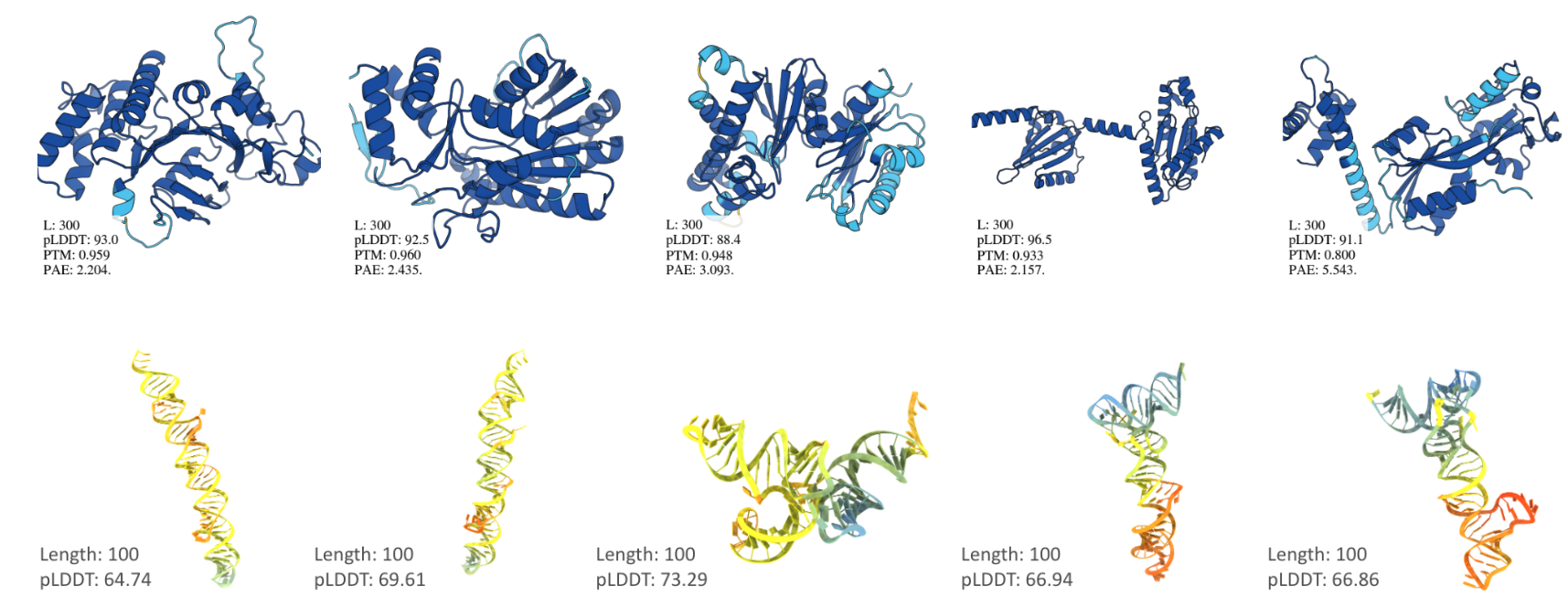
Figure 2: Visualizing the predicted structures of generated protein (top) and RNA (bottom) sequences. The protein structures are predicted by ESMFold (Lin et al., 2023) and the RNA structures are predicted by AlphaFold3 (Abramson et al., 2024). Additional structures depicted in Figure LABEL:fig:protein_structures_group1.

Setup and Evaluation. We benchmark our method against state-of-the-art protein sequence generation models, including discrete diffusion models (DPLM (Wang et al., 2024a), EvoDiff (Alamdari et al., 2024), and ESM3 (Hayes et al., 2025)), an autoregressive model (ProGen2 (Nijkamp et al., 2022)), and masked language models (ESM2 (Lin et al., 2023)). Each model generates 100 sequences across lengths in $[200,300,\dots,800]$, following their respective sampling strategies, with modifications ensuring fair evaluation. Protein sequence quality is assessed using ESMFold (Lin et al., 2023), measuring foldability through pLDDT, pTM, and pAE scores. We define foldability as the percentage of sequences satisfying pLDDT $>80$, pTM $>0.7$, and pAE $<10$. Additionally, we analyze token entropy and sequence diversity to detect mode collapse. Further details on experimental settings and evaluation metrics are provided in the Appendix LABEL:sec:protein_benchmark_eval.

Results. As summarized in Table 2, our P2 algorithm applied to DPLM (150M and 650M) consistently improves all folding metrics—pLDDT, pTM, and pAE—outperforming the default RDM sampling strategy (Zheng et al., 2023). Importantly, this improvement does not compromise token entropy or sequence diversity, highlighting P2’s ability to maintain diversity while enhancing quality.

When compared to baselines, including the 2.7B ProGen2-Large autoregressive model and discrete diffusion counterparts ESM3 and EvoDiff, P2 demonstrates remarkable foldability improvements. Visualizations of predicted structures for generated sequences are shown in Figure 2, illustrating P2’s ability to generate highly foldable, structurally plausible proteins. Detailed performance comparisons across sequence lengths are provided in Figure LABEL:fig:perf_vs_len. Overall, these results motivated us to experimentally validate generated sequences.

4.2 The Design Space of Path Planning

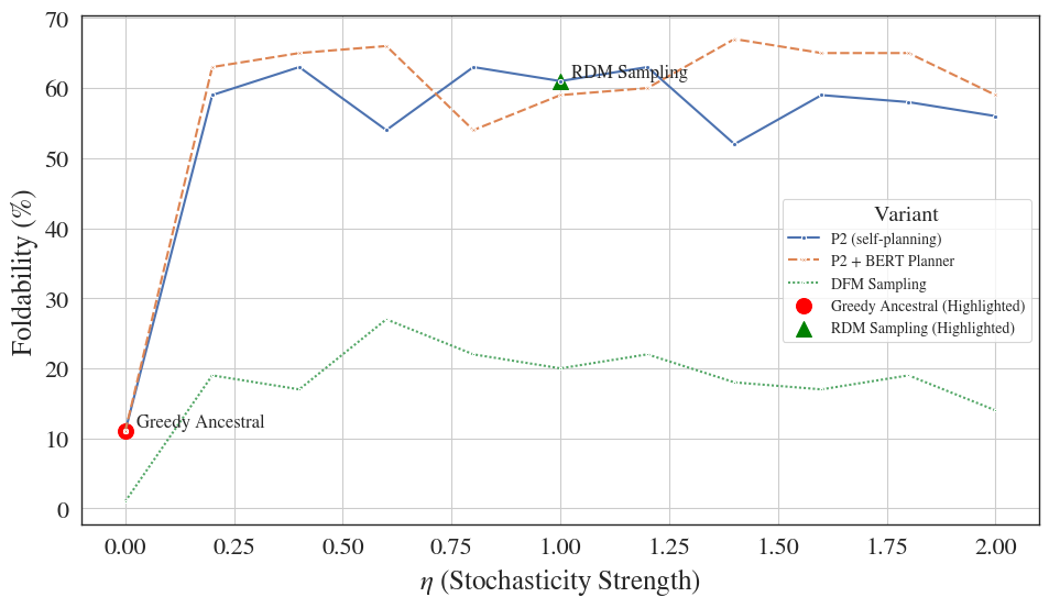
Figure 3: The Design Space of P2 (See Figure LABEL:fig:appendix_design_space_p2 for more). P2 Generalizes existing sampling algorithms with specific stochasticity strength and planner choice.

Our Path Planning (P2) framework generalizes existing sampling strategies, including vanilla ancestral sampling, greedy ancestral sampling, RDM sampling, and DFM sampling, by incorporating specific parameterizations. In Figure 3, we instantiate these sampling algorithms and evaluate their performance on protein sequence generation, focusing on foldability (additional metric results are provided in Figure LABEL:fig:appendix_design_space_p2).

Vanilla and greedy ancestral sampling employ a stochasticity strength of 0, effectively disabling remasking, which results in poor performance. DFM sampling introduces tunable stochasticity, leading to improved performance over ancestral sampling; however, it lacks trajectory planning, which limits its effectiveness. RDM sampling, by contrast, enables remasking with a default stochasticity strength of 1 and utilizes the denoiser’s confidence for self-planning, yielding better sampling quality.

P2 combines the advantages of these existing algorithms, offering both controllable stochasticity strength and planning guidance. By tuning stochasticity strength, P2 can enhance RDM sampling and optionally leverage an external BERT planner to further steer the sampling trajectory toward generating high-quality sequences.

4.3 Ablation of Path Planning

Table 3: Ablation of Sampling Strategies. Path planning (P2) outperforms existing sampling strategies, including DDPD. The arrows indicate whether higher (↑) or lower (↓) values are better.

Sampling Algorithm	pLDDT (↑)	pTM (↑)	pAE (↓)	Foldability (%) (↑)	Entropy (↑)	Diversity (%) (↑)
Vanilla Ancestral	44.08	0.34	20.61	2.00	4.03	93.63
RDM Sampling	74.67	0.71	10.33	43.00	3.85	93.12
P2 + 8M BERT Planner	78.24	0.74	9.11	44.50	3.80	92.77
DDPD + 8M BERT Planner	46.51	0.24	23.20	0.25	0.31	51.69
Ancestral	52.67	0.46	17.64	7.75	3.98	93.42

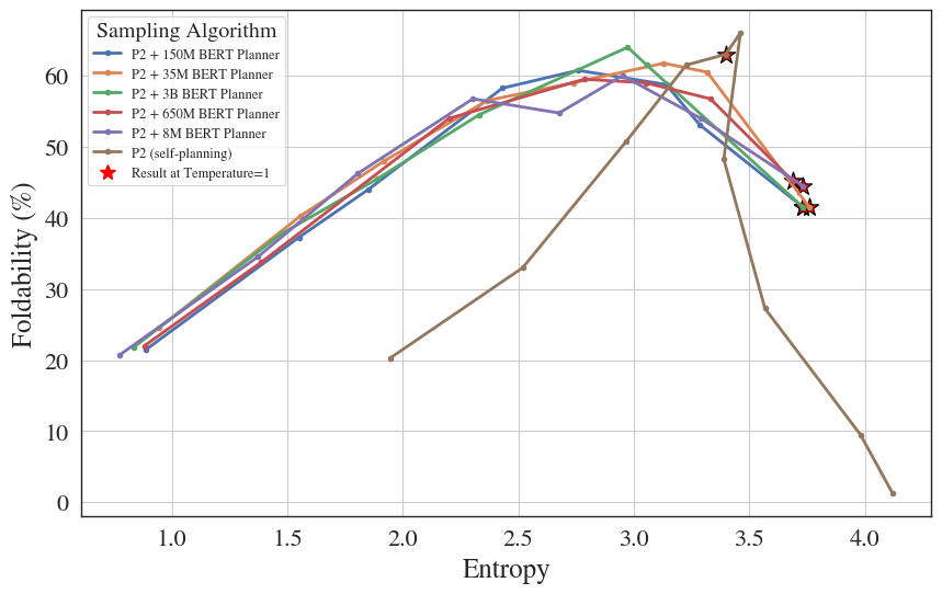
Figure 4: Ablation of the Planner Size: an 8M BERT planner functions similarly to a 3B BERT. Self-planning performs better in a default temperature of 1. We sweep the temperature from 0.1 to 2.0 and plot the scaling between the resultant sequence entropy and the foldability. For more see Figure LABEL:fig:more_ablation_planner.

Table 4: Comparison of negative ELBOs for Path Planning Planners and self-planning, averaged on 20 runs. Lower values ($\downarrow$) indicate better ELBO. The ELBO is computed at default temperature 1, corresponding to the star-annotation results in Figure 4.

Method	Unmasked pos.-ELBO ($\downarrow$)	Masked pos.-ELBO ($\downarrow$)
P2 + Planner ESM2-8M	22.5	13.4
P2 + Planner ESM2-35M	22.0	13.4
P2 + Planner ESM2-150M	21.8	13.4
P2 + Planner ESM2-650M	21.7	13.4
P2 + Planner ESM2-3B	21.6	13.4
P2 (self-planning)	15.7	13.4

Table 5: Ablation study of self-planning. We compare self-planning using denoiser-predicted probabilities with a uniformly sampled probability baseline. finetuned MDM refers to MDM fine-tuned from BERT (DPLM-150M (Wang et al., 2024a)), while tfs-MDM refers to MDM trained from scratch.

Configuration	pLDDT (↑)	pTM (↑)	pAE (↓)	Foldability (↑)	Entropy (↑)	Diversity (↑)
finetuned MDM	82.62	0.72	9.15	63.00	3.40	93.05
finetuned MDM + Uniform	72.61	0.66	11.82	39.00	4.01	93.62
tfs-MDM	74.67	0.71	10.33	43.00	3.85	93.12
tfs-MDM + Uniform	59.88	0.52	15.57	20.00	4.00	93.57

In this section, we utilize the protein sequence generation task as an ablation benchmark to analyze the implications of our Path Planning (P2) design choices. We experiment with the ESM2 (Lin et al., 2023) family of protein language models, including versions with 8M, 35M, 150M, 650M, and 3B parameters, for variants incorporating a BERT planner. For the denoiser, we train a 150M MDM from scratch, using the same architecture as ESM2-150M and DPLM-150M, for 500k steps with approximately 320k tokens per step. Training details are provided in Appendix LABEL:sec:training-detail-MDM-protein.

Results. Table 3 demonstrates that our P2 approach consistently outperforms existing sampling strategies across all folding metrics, while maintaining strong token entropy and sequence diversity. Notably, results are further enhanced when an external BERT planner is utilized. To provide a comparative perspective, we perform an apple-to-orange evaluation against a planner-based sampling algorithm, DDPD, equipped with the same BERT planner. DDPD is prone to generating low-entropy, repetitive sequences with poor foldability, as it relies exclusively on the planner to dictate both unmasking and remasking. In contrast, P2 separates these responsibilities: remasking is delegated to the BERT planner, while unmasking is guided by the denoiser itself. This decomposition mitigates the planner’s bias and leverages the denoiser’s planning capabilities effectively.

In Figure 4, we ablate the size of the planner and evaluate foldability under varying temperatures (entropy). Additional metric results are shown in Figure LABEL:fig:more_ablation_planner. Our findings reveal that an 8M BERT planner is sufficient to guide a 150M MDM, achieving competitive performance relative to its 3B counterpart across a broad range of entropy values. Furthermore, the BERT planner demonstrates superior scalability compared to the self-planning variant, preserving foldability under extreme high and low temperature conditions.

Self-Planning Analysis. In our self-planning approach, we leverage the predicted probabilities from unmasked positions to guide unmasking decisions. This raises a key question: Are the predicted probabilities from unmasked tokens meaningful? We conducted an ablation study where we replaced predicted probabilities for unmasked tokens with uniformly random values and performed the experiments on two MDM variants: one trained from scratch and another fine-tuned from a BERT-based model (DPLM-150M (Wang et al., 2024a)). The DPLM-150M was fine-tuned from ESM2, which was pretrained to predict both masked and randomly mutated tokens, making it more likely to inherit meaningful logits for unmasked positions. As shown in Table 5, randomizing unmasked token probabilities leads to a substantial decline in performance across both variants. This finding confirms that unmasked token logits are informative, despite the lack of direct supervision. It is also evidenced by the ELBO from Proposition 1 in Table 4 where self-planning displays an even better ELBO compared with BERT planners, further validating its effectiveness.

4.4 Sampling Efficiency

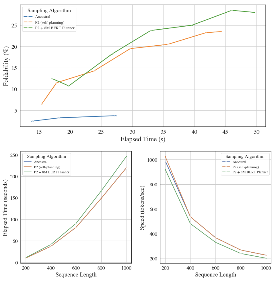
Figure 5: Top: Performance vs. Sampling Time (steps). Bottom: Running Time (left) and Speed (right) vs. Sequence Length.

Increasing the number of sampling steps generally enhances generative quality, albeit with increased computational time. To evaluate the scaling efficiency, we benchmark three sampling algorithms—ancestral sampling, P2 (self-planning), and P2 augmented with an 8M BERT planner—on the task of protein sequence generation. We measure the foldability across increasing sampling steps in terms of elapsed time (benchmarked on NVIDIA A100 GPUs). In Figure 5 top, P2 achieves superior foldability compared to ancestral sampling, while the inclusion of the external BERT planner demonstrates exceptional scalability, particularly at higher sampling steps. In Figure 5 bottom, we further analyze inference efficiency by examining elapsed time and speed (tokens per second) as a function of sequence length. P2 with self-planning maintains the same inference cost as ancestral sampling, as it does not rely on an external model. Conversely, P2 with the BERT planner doubles the number of sampling steps due to one additional BERT evaluation. However, since the planner is a lightweight 8M model compared to the 150M MDM, the overhead is negligible. This is evident in the figure, where the performance gap between P2 (self-planning) and P2 with the 8M BERT planner becomes indistinguishable at higher sampling scales.

4.5 Language Generation

Table 6: Language generation benchmarks, including reading comprehension (TriQA), last word completion task (LAMBADA), math reasoning (GSM8K), story infilling (ROCStories), and code generation. Baseline results are adopted from (Nie et al., 2024; Gong et al., 2024). For the infilling task, we use ROUGE-1/2/L score; for other tasks, we use the accuracy (%) metric. We employ P2 for the MDMs (1.1B) (Nie et al., 2024) and DiffuLLama (7B) (Nie et al., 2024) and show consistent improvement.

Model	TriQA (↑)	LAMBADA (↑)	GSM8K (↑)	ROCStories (↑)	Code (↑)
GPT2-S (127M)	4.0	25.9	44.8	(7.8/0.8/7.4)	1.6
DiffuGPT-S (127M)	2.0	45.0	50.2	13.7/1.4/12.6	0.3
SEDD-S (170M)	1.5	12.4	45.3	11.9/0.7/10.9	0.7
GPT2-M (355M)	6.7	37.7	50.7	(8.6/0.9/8.2)	2.6
DiffuGPT-M (355M)	3.8	60.5	52.6	18.7/2.7/17.0	2.9
SEDD-M (424M)	1.8	23.1	53.5	13.1/1.4/12.2	0.5
Plaid1B (1.3B)	1.2	8.6	32.6	12.1/1.1/11.2	0.1
TinyLlama (1.1B)	-	43.22	-	-	-
GPT-2 (1.5B)	-	44.61	-	-	-
Llama-2 (7B)	45.4	68.8	58.6	(11.6/2.1/10.5)	1.7
MDM (1.1B)	-	52.73	58.5	-	-
MDM (1.1B) + P2	-	52.88	60.9	-	-
DiffuLLama (7B)	18.5	53.72	-	20.31/2.83/18.16	13.2
DiffuLLama (7B) + P2	18.8	54.80	-	25.44/7.10/23.41	17.6

It has been widely pointed out that the existing evaluation such as toy datasets and NLL in text generation can be easily gamed to achieve low perplexity (Zheng et al., 2024a). In our evaluation, we follow the language benchmarking from SMDM (Gong et al., 2024) and DiffuLLama (Nie et al., 2024), and investigate the capabilities of MDMs in real-world evaluation language generation tasks that have been largely overlooked in prior works (Austin et al., 2021; Lou et al., 2023; Sahoo et al., 2024; Shi et al., 2024). We additionally provide the experiments of breaking the reverse curse in the Appendix LABEL:sec:BREAKING_THE_REVERSE_CURSE.

Benchmarks. We consider TriviaQA (Joshi et al., 2017) to test the reading comprehension of models and the last word completion task Lambada (Paperno et al., 2016) to test how models capture long-range dependencies in text. These two tasks are measured by exact match accuracy, i.e., given a prompt, we use MDMs to generate responses and calculate matching accuracy against the ground truth. Additionally, we employ complex tasks such as GSM8K (Cobbe et al., 2021), grade school math problem, to assess the math reasoning and story-infilling task using ROCStories (Mostafazadeh et al., 2016) and evaluate using ROUGE score (Lin, 2004). To test the code infilling, we also adopted Humaneval (Bavarian et al., 2022) single line infilling task, which is evaluated by pass@1 rate. We employ Language Model Evaluation Harness framework (Biderman et al., 2024) for performance assessment.

Baselines. We adopt the baselines and their results from previous works (Nie et al., 2024; Gong et al., 2024), including continuous diffusion model Plaid1B (1.3B) (Gulrajani & Hashimoto, 2023), discrete diffusion model SEDD-S (170M), SEDD-M (424M) (Lou et al., 2023), MDM (1B) (Gong et al., 2024), DiffuLLama(7B) (Nie et al., 2024), DiffuGPT-S (127M), DiffuGPT-M (355M) (Nie et al., 2024), and autoregressive models GPT2-S (127M), GPT2-M (355M), GPT-2 (1.5B) (Radford et al., 2019), TinyLlama (1.1B) (Zhang et al., 2024) and Llama-2 (7B) (Touvron et al., 2023).

Setup. We equip existing mask diffusion models MDM (1.1B) and DiffuLLama (7B) with our path planning and compare them with the default ancestral sampling results. For P2, we sweep the stochasticity strength from 0 to 2.0 with a step size of 0.2 and report the best results.

Results. As shown in Table 6, equipping with P2, we consistently improve the generation performance in the five benchmarks. In tasks that require more extensive global bidirectional reasoning, math reasoning GSM8K story infilling ROCStories, and code generation, P2 consistently exhibits improved performance by a large margin compared to the ancestral sampling. Compared to AR models that rely solely on left-toright modeling capabilities, P2 presents impressive generation accuracy; in code generation, where P2 achieves 17.6% pass@1 rate (vs. 1.7% of respective autoregressive model Llama-2 (7B)). In math reasoning, P2 enables a 1.1B-parameter MDM to outperform 7B-parameter Llama2 (60.9% vs. 58.5%). We attribute the success of P2 in complex language generation task to the remasking that corrects potential mistakes made in previous steps and promotes MDMs to generate robust answers.

4.6 RNA Sequence Generation

Table 7: RNA Sequence Generation Benchmark. The ”Native” row represents subsampled natural RNA sequences. ”MDM” refers to a pretrained 150M Masked Diffusion Model trained on RNACentral (Petrov, 2021).

Sequence Source	pLDDT (↑)	MFE (kcal/mol) (↓)	Entropy (↑)	GC Content (%) (↑)
Native	48.26	-35.83	1.96	49.64
RiNALMo-150M	59.01	-30.12	1.29	29.50
RiNALMo-650M	46.99	-31.90	1.33	28.06
MDM + Ancestral	68.12	-48.46	1.93	60.84
MDM + RDM	67.35	-47.54	1.89	59.42
MDM + P2 (self-planning)	69.41	-48.21	1.89	59.84
MDM + P2 + Planner RiNALMo-150M	73.28	-51.91	1.86	65.47

Experimental Setup. We train a 150M Masked Diffusion Model (MDM) trained on 27M RNA sequences from RNACentral (Petrov, 2021) over 100K steps with a batch size of 320K tokens.

We adopted the protein sequence evaluation protocols, using an external folding model (Shen et al., 2024) to estimate structural quality via pLDDT. We additionally calculate the Minimum Free Energy (MFE), GC Content (%), and sequence entropy. We generate 100 RNA sequences of 100 base pairs (bp) each. Visualizations are described in Appendix LABEL:sec:rna_vis.

Baselines. Two RNA language models, RiNALMo-150M and RiNALMo-650M (Penić et al., 2024), served as primary language model baselines. Additionally, a reference set of 100 native 100-bp RNA sequences was included for comparative purposes. We apply the existing sampling strategies along with the two P2 variants self-planning and BERT-planning (RiNALMo-150M) to the MDM. We evaluated stochasticity parameters ranging from 0 to 2 in 0.02 increments.

Results. As summarized in Table 7, self-planning outperforms native sequences baseline models (RiNALMo), and existing sampling strategies. Employing the RiNALMo planner further improves the key metrics, including pLDDT, predicted minimum free energy (MFE), and GC content with slight compromises in MFE and GC content.

5 Conclusion

We demonstrated that unmasking order significantly impacts the generative performance of masked diffusion models (MDMs). By expanding the ELBO formulation, we introduced a planner that optimizes token selection during inference. We proposed Path Planning (P2), a sampling framework that generalizes all existing MDM sampling strategies. P2 delivers state-of-the-art improvements across diverse tasks, including language generation and biological sequence design, enabling MDMs to outperform larger autoregressive models. Our findings highlight the importance of inference strategies in discrete diffusion models, paving the way for more efficient and effective sequence generation.

6 Acknowledgments

Fred extends sincere gratitude to Jiaxin Shi, Xinyou Wang, Zaixiang Zheng, Chengtong Wang, and Bowen Jing, Kaiwen Zheng for their invaluable insights on DPLM. Fred devotes his special thank-you to Tian Wang for playing ping-pong with him during the project. Zack likewise extends his gratitude to Jim Nolen for his invaluable insights.

The authors acknowledge funding from UNIQUE, CIFAR, NSERC, Intel, and Samsung. The research was enabled in part by computational resources provided by the Digital Research Alliance of Canada (https://alliancecan.ca), Mila (https://mila.quebec), and NVIDIA.

7 Author Contributions

F.Z.P. proposed the initial idea and conducted the experiments on language and protein modeling. Z.B. formulated the mathematical framework. S.P. carried out the experiments on RNA. F.Z.P. and Z.B. jointly wrote the manuscript, with all other authors contributing revisions and refinements. A.T., S.Y., and P.C. supervised the project.

8 Impact Statement

We introduce Path Planning (P2), a principled framework for optimizing the sampling order in masked diffusion models (MDMs), improving their generative quality across diverse sequence modeling tasks. By integrating path planning into the diffusion sampling process, P2 corrects early-stage errors, enhances sample fidelity, and generalizes existing sampling strategies. Our results demonstrate that P2 significantly improves state-of-the-art performance in protein and RNA sequence generation, as well as in language modeling applications such as reasoning and code generation. However, like any powerful generative method, P2 carries potential risks, including unintended applications in adversarial sequence design. We encourage responsible use and ethical oversight to ensure that P2 advances beneficial scientific and medical discoveries while mitigating risks of misuse.

Appendix

Appendix A Reproducibility Statement

We provide the PyTorch implementation in Appendix Section E. For the experiments, we integrate our approach into the SMDM (Gong et al., 2024) GitHub codebase to obtain the results for ”MDM (1.1B) + P2” reported in Table 6. Similarly, the results for ”DiffuLLaMA (7B) + P2” in Table 6 are derived using the DiffuLLaMA (Nie et al., 2024) GitHub codebase. For the protein sequence generation experiments, we utilize the DPLM (Wang et al., 2024a) open-source codebase. The RNA sequence generation results are obtained by adapting the DPLM codebase for MDM training, combined with the RiNALMo (Penić et al., 2024) language model architecture.

Appendix B Related Works

Masked Diffusion Models (MDMs) represent a promising alternative to autoregressive models for discrete data generation, particularly in language modeling. Recent advancements have focused on simplifying and generalizing the MDM framework to improve performance and training efficiency (Shi et al., 2024; Sahoo et al., 2024). These studies introduced a continuous-time variational objective for MDMs, expressed as a weighted integral of cross-entropy losses, facilitating the training of models with state-dependent masking schedules. At the GPT-2 scale, these MDMs outperformed prior diffusion-based language models and demonstrated superior capabilities in zero-shot language modeling tasks (Nie et al., 2024; Gong et al., 2024).

MDMs generate sequences starting from a fully masked input and progressively unmasking positions until a clean sequence is reached. Once a token is unmasked, it will stay unchanged. However, there is not guarantee that the state is correct, considering the approximation errors arise from the imperfect fit to real-world data distributions. Additionally, time discretization (Zhao et al., 2024) and numerical errors (Zheng et al., 2024b) may further the error incurred during sampling processes.

To address these challenges, several solutions have been proposed. These include methods allowing models to revise prior predictions and guiding sampling trajectories using internal or external knowledge. Examples include informed correctors (Zhao et al., 2024), greedy ancestral methods (Gong et al., 2024), and RDM sampling techniques (Zheng et al., 2023; Wang et al., 2024a), which leverage model scores to replace random masking with targeted corrections. None of these works, however, allow for the use of an external planner, and  (Zheng et al., 2023; Wang et al., 2024a) are simply using a top-k sampling strategy without any concern for the theoretical underpinnings of the sampling strategies viability.

In terms of theoretically-backed methods for selecting the denoising order during a generative model’s sampling process, the current literature is quite sparse. (Shih et al., 2022; Li et al., 2021) discuss this task from the perspective of Any-Order Autoregressive models, with (Li et al., 2021) requiring a specially-trained external planner model using a specially designed architecture and Shih et al. (2022) taking the perspective that a fixed family of possible generation orders should be chosen a priori to eliminate redundancy.

The most closely related work to ours is likely the recent DDPD (Liu et al., 2024) introduced a generative process divided into a planner, which identifies corrupted positions, and a denoiser, which refines these positions. Though they discuss the ability to employ a MDM denoiser within their framework, their analysis and sampling is through the lens of uniform discrete diffusion models. In particular, as with (Li et al., 2021), the success of their strategy is contingent upon training a large specialized planner model of comparable size to the denoiser itself. Moreover, in their framework, since they are based on uniform diffusion models, the partially de-noised sequence never contains any masked states, and there is no way for the planner to be separated into masked and unmasked components to design a sampling strategy with guaranteed finite-time along the lines of our Algorithm 1. Given the possible perceived similarity of this concurrent work with ours, we provide a thorough comparison of DDPD with P2 in Appendix 3, highlighting the greater flexibility and difference in role of P2s’ planners.

Appendix C Additional Background

C.1 Discrete Diffusion/Flow Models: Problem Setup

Here we discuss the general formulation of the problem setup and motivation behind discrete diffusion (Austin et al., 2021; Lou et al., 2023; Sun et al., 2022; Campbell et al., 2022) and discrete flow models (Campbell et al., 2024; Gat et al., 2024). This helps contextualize this manuscript in the broader landscape of the generative modeling framework, as well as introduce some additional notation that will be useful for the mathematical derivations in Appendix D.

Suppose we have a set if $N$ tokens, $S=\{1,\ldots,N\}$, and samples of sequences of length $L$ comprised of elements of $S$ from some distribution $p_{data}\in\mathcal{P}(S^{L})$. We seek to generate new samples from $p_{data}$ via learning a “denoising” function $D^{\theta}$ which allows one to sample from $p^{\theta}\approx p_{data}$.

To find such a function, we choose a family of probability measures $\{P_{t}(\cdot;\mu)\}_{t\in[0,1],\mu\in\mathcal{P}(S^{L})}$ such that $P_{0}(\cdot;\mu)=\mu$ and $P_{1}=\pi$, where $\pi\in\mathcal{P}(S^{L})$ is some easily-sampled from reference distribution. Then we find $\{\overset{\leftarrow}{X}_{t}\}_{t\in[0,1]}$ a continuous-time Markov chain with $\mathbb{P}(\overset{\leftarrow}{X}_{t}=x)=\overset{\leftarrow}{P}(x;p_{data})\coloneqq P_{1-t}(x;p_{data})$, and seek to use the “denoising function” $D^{\theta}$ to simulate a continuous time Markov chain $\{X^{\theta}_{t}\}_{t\in[0,1]}$ which is close in distribution to $\overset{\leftarrow}{X}$. In the end, we will have that taking $X^{\theta}_{0}\sim\pi$ and simulating the chain to time 1, $X^{\theta}_{1}\overset{d}{\approx}\overset{\leftarrow}{X}_{1}\sim p_{data}$. To understand what this process $X^{\theta}$ is and why the use of this intermediary Markov chain is useful for finding a choice of $D^{\theta}$, we first briefly review the theory of continuous time Markov chains in Appendix C.2.

C.2 Time-Inhomogeneous Continuous Time Markov Chains (CTMC)

A (time-inhomogenous) continuous-time Markov chain $\{X_{t}\}_{t\geq 0}$ on a finite set $\mathcal{X}$ is a stochastic process satisfying the Markov property, which can be formally summarized $\mathbb{P}(X_{t}=y|X_{s_{1}}=x_{1},\ldots,X_{s_{k}}=x_{k},X_{s}=x)=\mathbb{P}(X_{t}=y|X_{s}=x),\forall y,x_{1},\ldots,x_{k},x\in\mathcal{X},0\leq s_{1}<s_{2}<\ldots<s_{k}<s<t\leq 1$. One can construct such a process by specifying a ”rate matrix” $Q_{t}\in{\mathbb{R}}^{|\mathcal{X}|\times|\mathcal{X}|}$ with $Q_{t}(y,x)>0$ and $Q_{t}(x,x)=-\sum_{y\neq x}Q(y,x)$ for all $x\neq y\in\mathcal{X}$ and $t\geq 0$. Along with an initial distribution $\mu\in\mathcal{P}(\mathcal{X})$, $Q$ determines the 1-dimensional time marginals $\mathbb{P}(X_{t}=\cdot)\in\mathcal{P}(\mathcal{X})$ via the Kolmogorov equation:

$$\frac{d}{dt}\mathbb{P}(X_{t}=\cdot) =Q_{t}\mathbb{P}(X_{t}=\cdot),\qquad t\geq 0$$ (6)

$$\mathbb{P}(X_{0}=x) =\mu(x),\qquad x\in\mathcal{X}.$$

When the above holds, we will say $Q$ “generates” $X$. Note that one can see necessarily that if $Q$ generates $X$, $Q_{t}(y,x)\coloneqq\lim_{s\downarrow t}\frac{d}{ds}\mathbb{P}(X_{s}=y|X_{t}=x),x\neq y\in\mathcal{X}$. Knowing the entries of $Q$ also provides a means of generating samples from $X_{t}$ at any given time, since paths of $\{X_{t}\}_{t\geq 0}$ can be realized via a sequence of jump times $\{\tau_{n}\}_{n\in\mathbb{N}}$, with $\tau_{i}=\inf\{t>\tau_{i-1}:X_{t}\neq X_{\tau_{i-1}}\}$ and the effective discrete-time jump process $\{X_{\tau_{i}}\}_{i\in\mathbb{N}}$. Then

$$\mathbb{P}(X_{\tau_{i+1}}=y|X_{\tau_{i}}=x,\tau_{i}=t)=-\frac{Q_{t}(y,x)}{Q_{t}(x,x)},$$ (7)

and

$$\log(\mathbb{P}(\tau_{i+1}>t|X_{\tau_{i+1}}=x,\tau_{i}=s))=\int_{s}^{t}Q_{p}(x,x)dp.$$

For more background on time-inhomogenous continuous-time Markov chains, see e.g. Chapter 2 of (Yin & Zhang, 2013) or the appendix of (Ren et al., 2024).

C.3 The Role of the Denoiser and the Approximate Backwards Process

In the “discrete diffusion model” framework, one in fact starts with specifying a rate matrix $Q_{t}$ generating some Markov chain $\{X_{t}\}_{t\in[0,1]}$ with $X_{0}\sim p_{data}$ and $X_{1}\sim\pi$ and defines $P_{t}(x;p_{data})\coloneqq\mathbb{P}(X_{t}=x)$. $\overset{\leftarrow}{X}_{t}$ is then simply defined as $X_{1-t}$, and a rate matrix $\overset{\leftarrow}{Q}_{t}$ which generates $\overset{\leftarrow}{X}$ can be found from $Q_{t}$ via an application of Bayes’ rule (see Prop. 3.2 in (Sun et al., 2022)). In the “Discrete Flow Model” framework, one instead starts with a desired interpolation $P_{t}(\cdot;p_{data})$ between $p_{data}$ and $\pi$, and constructs a rate matrix $\overset{\leftarrow}{Q}_{t}$ generating a $\overset{\leftarrow}{X}_{t}$ with one-dimensional time marginals $\overset{\leftarrow}{P}_{t}(\cdot;p_{data})$ a posteriori.

As explained above, in order to generate samples of $\overset{\leftarrow}{X}_{t}$ at a given time (and in particular of $\overset{\leftarrow}{X}_{1}\sim p_{data}$), it is sufficient to have access to the entries of $\overset{\leftarrow}{Q}_{t}$. In both settings, however, the entries of $\overset{\leftarrow}{Q}_{t}$ will naturally depend on the unknown distribution $p_{data}$, and hence, using the form of this dependence, a the denoiser function $D^{\theta}$ is constructed in an attempt to approximate these unknown quantities. This results in a rate matrix $Q^{\theta}_{t}\approx\overset{\leftarrow}{Q}_{t}$, which generates the approximate backwards Markov chain $\{X^{\theta}_{t}\}_{t\in[0,1]}$. The distribution of the output of the resulting sampling scheme is then

$$p^{\theta}=P^{\theta}_{1}=\mathbb{P}(X^{\theta}_{1}=\cdot).$$

The form of the denoiser, as well as the choice of $P_{t},\overset{\leftarrow}{Q},$ and $Q^{\theta}$ in our particular setup are introduced in Sections 2.1 and 2.1.

C.4 The Conditional Backwards Process

A pervasive assumption made in the literature is that for any fixed $x^{0}\in S^{L}$,

$$P_{t}(y;\delta_{x^{0}})=\prod_{i=1}^{L}p_{t}(y_{i}|x^{0}_{i})$$ (8)

for a family of probability measures $\{p_{t}(\cdot|x^{0}_{i})\}_{t\in[0,1]}\subset\mathcal{P}(S)$. We denote by $\overset{\leftarrow}{X}^{x^{0}}$ the “conditional backwards process,” on the point $x^{0}$, defined as the Markov chain with distribution $\mathbb{P}(\overset{\leftarrow}{X}^{x_{0}}_{t}=y)=\overset{\leftarrow}{P}(y;\delta_{x^{0}})$, and by $\overset{\leftarrow}{Q}^{x^{0}}$ its rate matrix. The coordinates $(\overset{\leftarrow}{X}^{x_{0}}_{1},\ldots,\overset{\leftarrow}{X}^{x_{0}}_{L})$ of $\overset{\leftarrow}{X}^{x_{0}}$ are thus assumed independent, and each described by a continuous-time Markov chain $\{\overset{\leftarrow}{x}^{i}_{t}\}_{t\in[0,1]}$ with rate matrix $\hat{\overset{\leftarrow}{Q}}^{x^{0}_{i}}_{t}\in{\mathbb{R}}^{N\times N}$ for $i=1,\ldots,L$, $t\in[0,1]$ that yields $\mathbb{P}(\overset{\leftarrow}{x}^{i}_{t}=y_{i})=\overset{\leftarrow}{p}_{t}(y_{i}|x^{0}_{i})$ for all $t\in[0,1]$ and $y_{i}\in S$. The hope in making this assumption is that each coordinate of $X^{\theta}_{t}\approx\overset{\leftarrow}{X}_{t}$ will be able to be simulated independently in parallel without introducing significant error (Sun et al., 2022).

$P_{t}(y;\mu)$ is taken to be linear in $\mu$, so we have $P_{t}(y;p_{data})=\sum_{x\in S^{L}}P_{t}(y;\delta_{x})p_{data}(x)$, and hence specifying $p_{t}(j|i),i,j\in S$ is what ultimately what determines the form of $\overset{\leftarrow}{Q}_{t}$ and hence the functions needed to be approximated by $D^{\theta}$ in order to construct $Q^{\theta}$. The most common choices explored this far in the literature are the “uniform diffusion,” (Lou et al., 2023; Schiff et al., 2024) which sets

$$p_{t}(j|i)=\alpha(t)\delta_{i}(j)+\frac{1-\alpha(t)}{S}$$ (9)

for $\alpha:[0,1]\rightarrow[0,1]$ with $\alpha(0)=1,\alpha(1)=0$ and the “masked diffusion,” which is out subject of focus.

Note that in the Discrete Diffusion Model framework, $p_{t}(j|i)$ is not always defined explicitly, and is often implicitly prescribed by asserting the “forward noising” process is the independent evolution of a CTMC on $S$ with rate matrix $\hat{Q}_{t}\in{\mathbb{R}}^{N\times N}$ on each coordinate (see e.g. Equations (15) and (16) in (Lou et al., 2023)). $p_{t}(j|i)$ is then found by solving Eq. 6 with $Q=\hat{Q}$ and $\mu=\delta_{i}$.

In the case of a “masked diffusion model,” one extends $S$ to $\bar{S}=S\cup\{M\}$ for $M$ some “masked state” outside the dictionary of tokens $S$, and takes:

$$p_{t}(j|i)=\alpha(t)\delta_{i}(j)+(1-\alpha(t))\delta_{M}(j),\quad i,j\in\bar{S}$$ (10)

for a monotone-decreasing, continuously differentiable noise scheduler $\alpha:[0,1]\rightarrow[0,1]$ with $\alpha(0)=1$ and $\alpha(1)=0$. This choice of forward/noising process has been seen to outperform the uniform diffusion process (Schiff et al., 2024) as well as other choices of $p_{t}$ (Austin et al., 2021) consistently among applications. If corresponds to the coordinate-wise forward matrix $\hat{Q}_{t}(j,i)=\sigma(t)\delta_{M}(j)(1-\delta_{M}(i)),i\neq j\in\bar{S}$ with $\sigma(t)=-\frac{d}{dt}\log(\alpha(t))$, and through Eq. 8 yields Eq. 1.

In the masked-diffusion setting, both the Discrete Flow Model and Discrete Diffusion Model framework use the rate matrices for the conditional reversed process’ coordinates ((Campbell et al., 2024) Appendix F.1.):

$$\hat{\overset{\leftarrow}{Q}}^{x^{0}_{i}}_{t}(j,i) =-\frac{\dot{\alpha}(1-t)}{1-\alpha(1-t)}\delta_{M}(i)\delta_{x^{0}_{i}}(j),\quad i,j\in\bar{S}.$$

The resulting conditional rate matrix generating $\overset{\leftarrow}{X}^{x^{0}}_{t}$ is then, for $x\neq y\in\bar{S}^{L}$:

$$\overset{\leftarrow}{Q}_{t}^{x^{0}}(y,x)=-\frac{\dot{\alpha}(1-t)}{1-\alpha(1-t)}\sum_{i=1}^{L}\delta_{M}(x_{i})\delta_{x^{0}_{i}}(y_{i})\delta_{y^{-i}}(x^{-i})$$ (11)

with $\overset{\leftarrow}{Q}_{t}^{x^{0}}(x,x)=\frac{\dot{\alpha}(1-t)}{1-\alpha(1-t)}\sum_{i=1}^{L}\delta_{M}(x_{i})$.

C.5 Role of the ELBO

The training objective in general is obtained via the same methodology in both the Discrete Flow and Discrete Diffusion Model framework – in fact this methodology can also be used for continuous diffusion models and denoising processes described by more general Markovian dynamics (Benton et al., 2024).

We seek to minimize the KL divergence:

$$D_{KL}(p_{data}||P^{\theta}_{1}) =\sum_{x\in S^{L}}p_{data}(x)\log\left(\frac{p_{data}(x)}{P^{\theta}_{1}(x)}\right)$$

$$=\sum_{x\in S^{L}}p_{data}(x)\log p_{data}(x)-\sum_{x\in S^{L}}p_{data}(x)\log(P^{\theta}_{1}(x)).$$

The first term, the entropy of $p_{data}$ is constant in $\theta$, and so we turn our attention to finding an “Evidence Based Lower Bound”

$$E(x^{0})\leq\log(P^{\theta}_{1}(x^{0}))$$

for each fixed $x^{0}\in S^{L}$.The loss that we seek to minimize will is then defined as:

$$\mathcal{L}_{E}\coloneqq-\sum_{x\in S^{L}}p_{data}(x)E(x).$$ (12)

Letting $\mathbb{P}^{x}\in\mathcal{P}(D([0,1];S^{L}))$ denote the Law (on the Skorokhod space of all cádlág paths from $[0,1]$ to $S^{L}$) of $\overset{\leftarrow}{X}^{x^{0}}$ and $\mathbb{P}^{\theta}\in\mathcal{P}(D([0,1];S^{L}))$ the same but for $X^{\theta}$, we have, by the data-processing inequality (see, e.g. (Budhiraja & Dupuis, 2019) Lemma 2.4 (f)):

$$\log(P^{\theta}_{1}(x^{0}))=-D_{KL}(\delta_{x^{0}}||P^{\theta}_{1})\geq-D_{KL}(\mathbb{P}^{x^{0}}||\mathbb{P}^{\theta})\coloneqq E(x^{0}),$$

That is, in order to make sure the approximate reverse process has the desired terminal distribution, by minimizing $\mathcal{L}_{E}$ we attempt to make it so that the entire path of the approximate reverse process matches that of the exact one.

$E(x^{0})$ can be found via an application of Girsanov’s Theorem for Markov Jump processes (see e.g. Theorem III.5.34 in (Jacod & Shiryaev, 2013) for a general result or (Ren et al., 2024) Theorem 3.3 for the specific Markov Chain setting), and is expressed solely in terms of $\overset{\leftarrow}{Q}^{x^{0}}$, $D^{\theta}$, and $P_{t}(\cdot;\delta_{x})$. In the masked diffusion setting, where $Q^{\theta}$ is given by $Q^{\theta,\text{mask}}$ from Eq. 2 and $\overset{\leftarrow}{Q}^{x^{0}}$ is given by Eq. 11, this expression is ((Sahoo et al., 2024) Equation (10)):

$$E_{mask}(x^{0}) =-\int_{0}^{1}\frac{\dot{\alpha}(t)}{1-\alpha(t)}\mathbb{E}_{X_{t}\sim P_{t}(\cdot;\delta_{x^{0}})}\left[\sum_{i:[X_{t}]_{i}=M}\log(D_{i,x^{0}_{i}}^{\theta}(X_{t}))\right]dt,$$ (13)

with $P_{t}$ as in Eq. 1. This is exactly $E_{D}$ from Proposition 1.

Appendix D Mathematical Details

D.1 Equivalence of MDMs with AOARMs

Here, for completeness, we recall the connection between Masked Diffusion Models and Any-Order Autoregressive Models (Uria et al., 2014; Hoogeboom et al., 2022) as described in (Zheng et al., 2024b; Ou et al., 2024). We start by providing a simplified derivation of the equivalence of the two types of models’ sampling schemes.

We begin by obtaining the diagonals for the matrix Eq. 2. Recalling $D^{\theta}_{i,y_{i}}(x)=\delta_{x_{i}}(y_{i})$ if $x_{i}\neq M$, and $\sum_{y_{i}=1}^{N}D^{\theta}_{i,y_{i}}(x)=1$ if $x_{i}=M$:

$$-\sum_{y\neq x}Q^{\theta}_{t}(y,x) =\frac{\dot{\alpha}(1-t)}{1-\alpha(1-t)}\sum_{i=1}^{L}\delta_{M}(x_{i})\sum_{y_{i}\neq x_{i}}D_{i,y_{i}}^{\theta}(x)$$

$$=\frac{\dot{\alpha}(1-t)}{1-\alpha(1-t)}\sum_{i=1}^{L}\delta_{M}(x_{i})\sum_{y_{i}=1}^{N}D_{i,y_{i}}^{\theta}(x)$$

$$=\frac{\dot{\alpha}(1-t)}{1-\alpha(1-t)}\sum_{i=1}^{L}\delta_{M}(x_{i}).$$

Then, if one considers the effective jump chain’s transition probabilities as described in Eq. 7, we have, for $x\neq y$:

$$\mathbb{P}(X^{\theta,\text{mask}}_{\tau_{k+1}}=y|X^{\theta,\text{mask}}_{\tau_{k}}=x,\tau_{k}=t)=\mathbb{P}(X^{\theta,\text{mask}}_{\tau_{k+1}}=y|X^{\theta,\text{mask}}_{\tau_{y}}=x)=\frac{\sum_{i=1}^{L}\delta_{M}(x_{i})D_{i,y_{i}}^{\theta}(x)\delta_{y^{-i}}(x^{-i})}{\sum_{i=1}^{L}\delta_{M}(x_{i})}.$$

We note that this is zero when the Hamming distance $d_{HAM}(x,y)\neq 1$.

Then, for any $j\in\{1,\ldots,N\}$:

$$\mathbb{P}([X^{\theta,\text{mask}}_{\tau_{k+1}}]_{j}\neq[X^{\theta,\text{mask}}_{\tau_{k+1}}]_{j}|X^{\theta,\text{mask}}_{\tau_{k}}=x,\tau_{k}=t) =\sum_{y\in\bar{S}^{L}:y_{j}\neq x_{j}}\mathbb{P}([X^{\theta,\text{mask}}_{\tau_{k+1}}]_{j}=y|X^{\theta,\text{mask}}_{\tau_{k}}=x)$$

$$=\sum_{y\in\bar{S}^{L}:y_{j}\neq x_{j}}\frac{\sum_{i=1}^{L}\delta_{M}(x_{i})D_{i,y_{i}}^{\theta}(x)\delta_{y^{-i}}(x^{-i})}{\sum_{i=1}^{L}\delta_{M}(x_{i})}$$

$$=\sum_{y_{j}\neq x_{j}}\frac{\delta_{M}(x_{j})D_{j,y_{j}}^{\theta}(x)}{\sum_{i=1}^{L}\delta_{M}(x_{i})}$$

$$=\frac{\delta_{M}(x_{j})\sum_{y_{j}=1}^{N}D_{j,y_{j}}^{\theta}(x)}{\sum_{i=1}^{L}\delta_{M}(x_{i})}$$

$$=\frac{\delta_{M}(x_{j})}{\sum_{i=1}^{L}\delta_{M}(x_{i})}$$

and, for $x$ such that $x_{j}=M$:

$$\mathbb{P}([X^{\theta,\text{mask}}_{\tau_{k+1}}]_{j}=y^{\prime}_{j}|X^{\theta,\text{mask}}_{\tau_{k}}=x,\tau_{k}=t,[X^{\theta,\text{mask}}_{\tau_{k+1}}]_{j}\neq[X^{\theta,\text{mask}}_{\tau_{k+1}}]_{j})$$

$$=\frac{\mathbb{P}([X^{\theta,\text{mask}}_{\tau_{k+1}}]_{j}=y^{\prime}_{j},[X^{\theta,\text{mask}}_{\tau_{k+1}}]_{j}\neq[X^{\theta,\text{mask}}_{\tau_{k+1}}]_{j})|X^{\theta,\text{mask}}_{\tau_{k}}=x,\tau_{k}=t)}{\mathbb{P}([X^{\theta,\text{mask}}_{\tau_{k+1}}]_{j}\neq[X^{\theta,\text{mask}}_{\tau_{k+1}}]_{j})|X^{\theta,\text{mask}}_{\tau_{k}}=x,\tau_{k}=t)}$$

$$=\frac{\sum_{i=1}^{L}\delta_{M}(x_{i})}{\delta_{M}(x_{j})}\sum_{y\in\bar{S}^{L}:y_{j}=y^{\prime}_{j}\neq x_{j}}\mathbb{P}([X^{\theta,\text{mask}}_{\tau_{k+1}}]_{j}=y|X^{\theta,\text{mask}}_{\tau_{k}}=x)$$

$$=\sum_{y\in\bar{S}^{L}:y_{j}=y^{\prime}_{j}\neq x_{j}}\sum_{i=1}^{L}\delta_{M}(x_{i})D_{i,y_{i}}^{\theta}(x)\delta_{y^{-i}}(x^{-i})$$

$$=\delta_{M}(x_{j})D_{j,y^{\prime}_{j}}^{\theta}(x)$$

$$=D_{j,y^{\prime}_{j}}^{\theta}(x).$$

Defining for $x\in\bar{S}^{L}$, $M(x)\coloneqq\{j\in\{1,\dots,L\}:x_{j}=M\}$, the corresponding Gillespie sampling scheme (Gillespie, 1977, 1976) for a standard masked diffusion model is thus as follows:

Algorithm 2 Gillespie Sampler for Masked Diffusion Models

1:Initialize: $x_{0}\leftarrow(M,M,\dots,M)$, denoiser $D^{\theta}$

2:for $t=1:L$ do

3:  Choose Random Coordinate for Unmasking:

4:  Sample dimension $d^{\prime}\sim\operatorname{Unif}\big{(}M(x_{t})\big{)}$

5:  Denoise:

6:  Sample $y_{d^{\prime}}\sim D^{\theta}_{d^{\prime},\cdot}(x_{t})$

7:  $[x_{t+1}]_{d^{\prime}}\leftarrow y_{d^{\prime}}$

8:end for

9:return $x_{L}$

Letting $\mathbb{S}_{L}$ be the set of all permutations of $\{1,\ldots,L\}$, we then have:

$$\mathbb{P}(X^{\theta,\text{mask}}_{1}=x) =\frac{1}{L!}\sum_{\sigma\in\mathbb{S}_{L}}\prod_{i=1}^{L}D^{\theta}_{\sigma(i),x_{\sigma(i)}}(x^{-\sigma(\geq i),M})$$

$$=\mathbb{E}_{\sigma\sim\text{Unif}(\mathbb{S}_{L})}\left[\mathbb{P}(X^{\theta,\text{mask}}_{1}=x|\sigma)\right]$$

where $x^{\sigma(<i),M}\in\bar{S}^{L}$ is $x$ but with $x_{\sigma(j)}=M,\forall j\geq i$. Here $\sigma(i)$ represents the coordinate which is unmasked at time $\tau_{i}$. From this it is clear that with each unmasking, $D^{\theta}$ is gaining additional conditional information about the sequence it is denoising, and could potentially benefit from backtracking and remasking previously unmasked tokens.

Moreover, in (Ou et al., 2024), it is proved that the loss that $D^{\theta}$ is trained on (see Eq. 12 and Eq. 13) is equivalent to:

$$\mathcal{L}_{\text{mask}}(\theta) =-\mathbb{E}_{x\sim p_{data}}\left[\mathbb{E}_{\sigma\sim\text{Unif}(\mathbb{S}_{L})}\left[\log\left(\mathbb{P}(X^{\theta,\text{mask}}_{1}=x|\sigma)\right)\right]\right]$$

$$=\mathbb{E}_{\sigma\sim\text{Unif}(\mathbb{S}_{L})}\left[D_{KL}(p_{data}||\mathbb{P}(X^{\theta,\text{mask}}_{1}=\cdot|\sigma))\right]+H(p_{data}),$$

where $H$ is the Shannon Entropy of $p_{data}$. This is minimized with value $H(p_{data})$ if and only if $\mathbb{P}(X^{\theta,\text{mask}}_{1}=\cdot|\sigma)=p_{data},\forall\sigma\in\mathbb{S}_{L}$; that is, if every choice of unmasking order exactly recovers the data distribution.

It becomes clear that if the training objective used for a Masked Diffusion Model was made uniformly $0$, every choice of unmasking order would exactly recover the data distribution (the KL divergence is $0$ if and only if the distributions are equal - see e.g. (Budhiraja & Dupuis, 2019) Lemma 2.1). In practice, however, $D^{\theta}$ is far from perfect (and even if it were, it is trained using samples form $p_{data}$, so would just recover those samples). As such, not all such orders will be created equal - that is there will be denoising orders $\sigma,\hat{\sigma}\in\mathbb{S}_{L}$ such that

$$D_{KL}(p_{data}||\mathbb{P}(X^{\theta,\text{mask}}_{1}=\cdot|\sigma))>>D_{KL}(p_{data}||\mathbb{P}(X^{\theta,\text{mask}}_{1}=\cdot|\hat{\sigma})).$$

This was observed empirically in (Ou et al., 2024) Appendix G.4, (Shih et al., 2022), and (Li et al., 2021) Section 6.

D.2 Comparison with DDPD

As it the most similar work to ours in the existing literature, here we provide a thorough comparison with DDPD (Liu et al., 2024). Given that our objective is to plan a denoising order assuming access to a Masked Diffusion Model for our denoiser (as with DDPD-MaskD) and not to train a uniform diffusion-based denoiser from scratch (as with DDPD-DFM-Uni), we focus on their framework in the former setting.

Even with DDPD-MaskD, the framework uses a “uniform discrete diffusion” Eq. 9 as the starting-point for their token-wise forward noising process, as opposed to the “masked diffusion” forward noising process Eq. 10 used in our work. They modify the state space $S^{L}$ to $\tilde{S}^{L}$, where $\tilde{S}=S\times\{N,D\}$. Dor $(y,z)\in\tilde{S}^{L}$, $(y_{i},z_{i})$ denotes the pair describing the state $y_{i}\in S$ in of $i$’th token and $z_{i}\in\{N,D\}$ denotes whether that token is noise $(N)$ or data $(D)$. They then modify the forward noising process to:

$$p_{t}((j,\zeta)|i)=\alpha(t)\delta_{(i,D)}(j,\zeta)+\frac{1-\alpha(t)}{S}\delta_{N}(\zeta),\quad i,j\in S,\quad\zeta\in\{N,D\},$$

see Equation (17) therein.

Thus, their reference distribution $\pi\in\mathcal{P}(\tilde{S}^{L})$ is given by $\pi=\text{Unif}(S^{L})\otimes\delta_{N^{L}}$, where $N^{L}\in\{N,D\}^{L}$ consists of all $N$’s, and the corresponding backwards processes’ $S^{L}$ marginal is initialized at the $\text{Unif}(S^{L})$ as opposed to $\delta_{M^{L}}$ as in our setting.

They approximate a resulting true backward process on $S^{L}$’s rate matrix $\overset{\leftarrow}{Q}_{t}$ (given by Proposition 3.1 therein) with $Q^{\theta,\text{DDPD}}_{t}$ given by:

$$Q^{\theta,\text{DDPD}}_{t}(y,x) =-\frac{\dot{\alpha}(1-t)}{1-\alpha(1-t)}\sum_{i=1}^{L}G^{\theta,\text{DDPD}}_{i,N}(x)\mathbb{E}_{Z\sim G^{\theta}(x)}[D^{\theta}_{i,y_{i}}(x^{Z,-i,M})]\delta_{y^{-i}}(x^{-i})$$

where $D^{\theta}:\bar{S}^{L}\rightarrow\mathcal{P}(S)^{L}$ is a denosier for a masked diffusion model trained via the ELBO Eq. 13 as in Eq. 3. Here for $x\in S^{L}$, $z\in\{N,D\}^{L}$, $x^{z,-i,M}\in\bar{S}^{L}$ is obtained from $x$ via:

$$x^{z}_{j}=\begin{cases}M,&\quad z_{j}=N\\ x_{j},&\quad z_{j}=D,j\neq i\\ M,&\quad j=i\end{cases}.$$

$G^{\theta,\text{DDPD}}:S^{L}\rightarrow\mathcal{P}(\{N,D\})^{L}$ is another neural network with $G^{\theta,\text{DDPD}}_{i,N}(x)$ approximating the probability that the $i$’th coordinate of $x\in\mathcal{S}^{L}$ is noise, and is trained via Eq. 12 with $E(x^{0})=E^{\text{DDPD}}(x^{0})$ given by:

$$E^{\text{DDPD}}(x^{0}) =E^{\text{DDPD}}_{P}(x^{0})+E^{\text{DDPD}}_{D}(x^{0})$$

$$E^{\text{DDPD}}_{P}(x^{0}) =-\int_{0}^{1}\frac{\dot{\alpha}(t)}{1-\alpha(t)}\mathbb{E}_{(\tilde{X}_{t},Z_{t})\sim P^{\text{DDPD}}_{t}(\cdot|\delta_{(x^{0},D^{L})})}\biggl{[}\sum_{i=1}^{L}\log\left(G^{\theta,\text{DDPD}}_{i,[Z_{t}]_{i}}(\tilde{X}_{t})\right)\biggr{]}dt$$

$$E^{\text{DDPD}}_{D}(x^{0}) =-\int_{0}^{1}\frac{\dot{\alpha}(t)}{1-\alpha(t)}\mathbb{E}_{(\tilde{X}_{t},Z_{t})\sim P^{\text{DDPD}}_{t}(\cdot|\delta_{(x^{0},D^{L})})}\biggl{[}\sum_{i=1}^{L}\delta_{[Z_{t}]_{i}=N}\mathbb{E}_{\hat{Z}\sim G^{\theta,\text{DDPD}}(\tilde{X}_{t})}\left[\log\left(D^{\theta}_{i,x^{0}_{i}}(\tilde{X}_{t}^{\hat{Z},-i,M})\right)\right]\biggr{]}dt$$

$$P_{t}((y,z)|\delta_{(x^{0},D^{L})}) \coloneqq\alpha(t)\delta_{(x^{0},D^{L})}(y,z)+\frac{(1-\alpha(t))}{S^{L}}\delta_{N^{L}}(z),\qquad y\in S^{L},z\in\{N,D\}^{L}$$

Note that in the above ELBO, $E^{\text{DDPD}}_{D}$ is slightly modified from what which they present in Theorem 4.1. As written, they would take the expected value with respect to $G^{\theta,\text{DDPD}}$ inside the second $\log$, which requires $2^{L-1}$ function evaluations of $D^{\theta}$. When the denoiser $D^{\theta}$ is given by that of a masked diffusion, one should instead use the above, which can be readily arrived at the same proof with an extra application of Jensen’s inequality.

Comparing this with our Proposition Eq. 1, the comparison between DDPD and P2 becomes evident: $E^{\text{DDPD}}_{P}(x^{0})$ is playing the role of $E_{UP}(x^{0})+E_{MP}(x^{0})$ (that is, it yields the training objective for the Planner) and $E^{\text{DDPD}}_{D}(x^{0})$ is playing the role of $E_{D}(x^{0})$ (that is, it yields the training objective for the denoiser). However, we note the following key distinguishing factors:

1. In P2, $E_{D}$ is the same as the ELBO originally used to train the denoiser $D^{\theta}$: that is, $D^{\theta}$ has already be trained to maximize $\mathbb{E}_{x_{0}\sim p_{\text{data}}}[E_{D}(x^{0})]$. Meanwhile, $E^{\text{DDPD}}_{D}$ depends on the output of $G^{\theta,\text{DDPD}}$, increasing the importance of the role of planner in the quality of the generations output. For this reason, DDPD must train an external Planner whose model size is comparable to that of the denoiser - they are essentially asking the planner to play a role akin to the denoiser in a uniform diffusion model. Meanwhile, due to the “flipped” importance of the roles of the planner and denoiser in P2, we show that we can use lightweight BERT models or even the denoiser itself as an effective Planner. See Table 3, where we confirm DDPD’s inability to make use of such lightweight models.

2. In P2, we separate the Planner’s training objective into two components. This is natural because our planner may use information both from the partially masked data $X_{t}$ and the output of the denoiser $Y$. Meanwhile, in DDPD, the Planner only has access to $\tilde{X}_{t}$-unmasked data perturbed by random flips of its tokens. Because DDPD’s generation process is grounded in a uniform diffusion process, there is no ability to separate the Planner into unmasked and masked components as we do in Section Eq. 3.2. In particular, their framework does not allow for a general enough planner to introduce our stochasticity strength parameter $\eta$ and design an algorithm analogous to the P2 Sampler 1.

The practical differences between DDPD and P2 are further elucidated by comparing their Gillespie sampling strategy (Algorithm 1 therein) with ours (see Alg. 4). For convenience, we reproduce it here.

Letting $\hat{G}^{\theta,\text{DDPD}}:S^{L}\rightarrow\mathcal{P}(\{1,\ldots,L\})$ be given by $\hat{G}^{\theta,\text{DDPD}}_{j}(x)=\frac{G^{\theta,\text{DDPD}}_{j,N}(x)}{\sum_{j=1}^{L}G^{\theta,\text{DDPD}}_{j,N}(x)}$, DDPD’s Gillespie sampling algorithm is given by Alg. 3.

Algorithm 3 DDPD Sampler

1:init $i\leftarrow 0,x_{0}\sim\operatorname{Unif}(S^{L})$, planner $G^{\theta,\text{DDPD}}$, denoiser $D^{\theta}$, maximum steps $T$

2:for $t=1:T$ do

3:  Plan Sample dimension $d^{\prime}\sim\hat{G}_{\cdot}^{\theta,\text{DDPD}}(x_{t})$

4:  Denoise Sample $z\sim G^{\theta,\text{DDPD}}$

5:  Sample $y_{d^{\prime}}\sim D^{\theta}_{d^{\prime},\cdot}(x_{t}^{z,-i,M})$

6:  Update: $[x_{t+1}]_{d^{\prime}}\leftarrow y_{d^{\prime}}$

7:end for

8:return $x_{T}$

As is clear from Alg. 3, in DDPD, the input to the Planner only depends on some unmasked, randomly flipped sequence of tokens, and does not depend on the output of the denoiser, and the input to the denoiser is entirely dependent on the output of the planner. Meanwhile, in P2, the Planner may use the both the information about the partially unmasked sequence (whose unmasked tokens all result from samples from the denoiser) and the output of the denoiser, and the input to the denoiser only depends on the output of the planner insofar as it may choose to remask a single token.

D.3 Deriving the P2 Gillespie Scheme Alg. 4

Let $\{\tau_{k}\}_{k\in\mathbb{N}}$ be the jump times for the CTMC $X^{\theta}$ with rate matrix $Q^{\theta}$ as described in Equation Eq. 4 (see Appendix C.2). To derive a Gillespie sampling scheme, we need to find the transition probabilities for the effective jump chain as described in Eq. 7. We first need to obtain the diagonal entries for the jump matrix $Q^{\theta}$. We have for $x\in\bar{S}^{L}$:

$$-\sum_{y\neq x}Q^{\theta}_{t}(y,x) =\frac{\dot{\alpha}(1-t)}{1-\alpha(1-t)}\sum_{i=1}^{L}\sum_{y_{i}=1,y_{i}\neq x_{i}}^{N}F^{\theta}_{i,N}(y,x)\hat{D}^{\theta}_{i,y_{i}}(x)$$

$$=\frac{\dot{\alpha}(1-t)}{1-\alpha(1-t)}\sum_{i=1}^{L}\biggl{[}\delta_{M}(x_{i})\sum_{y_{i}=1,y_{i}\neq x_{i}}^{N}\mathbb{E}_{Z\sim D^{\theta}(x)}[G^{\theta}_{i}(Z^{-i,y_{i}})]D^{\theta}_{i,y_{i}}(x)$$

$$+\frac{(1-\delta_{M}(x_{i}))}{1-D^{\theta}_{i,x_{i}}(x^{-i,M})}\sum_{y_{i}=1,y_{i}\neq x_{i}}^{N}\mathbb{E}_{Z\sim D^{\theta}(x)}[G^{\theta}_{i}(Z^{-i,x_{i}},x)]D^{\theta}_{i,y_{i}}(x^{-i,M})\biggr{]}$$

$$=\frac{\dot{\alpha}(1-t)}{1-\alpha(1-t)}\sum_{i=1}^{L}\delta_{M}(x_{i})\mathbb{E}_{Z\sim D^{\theta}(x)}[G^{\theta}_{i}(Z,x)]+(1-\delta_{M}(x_{i}))\mathbb{E}_{Z\sim D^{\theta}(x)}[G^{\theta}_{i}(Z^{-i,x},x)]$$

$$=Q^{\theta}_{t}(x,x).$$

Then for $x\neq y\in\bar{S}^{L}$, $k\in\mathbb{N}$, and $t\in[0,1]$:

$$\mathbb{P}(X^{\theta}_{\tau_{k+1}}=y|X^{\theta}_{\tau_{k}}=x,\tau_{k}=t)=\frac{\sum_{i=1}^{L}F^{\theta}_{i}(y,x)\hat{D}^{\theta}_{i,y_{i}}(x)\delta_{y^{-i}}(x^{-i})}{\sum_{i=1}^{L}\delta_{M}(x_{i})\mathbb{E}_{Z\sim D^{\theta}(x)}[G^{\theta}_{i}(Z,x_{i})]+(1-\delta_{M}(x_{i}))\mathbb{E}_{Z\sim D^{\theta}(x)}[G^{\theta}_{i}(Z^{-i,x},x)]}.$$

We note that this is zero when the Hamming distance $d_{HAM}(x,y)\neq 1$ and independent of $t$ and $k$.

Then, for $j\in\{1,\ldots,N\}$ and $x,y,k,t$ as before:

$$\mathbb{P}([X^{\theta}_{\tau_{k+1}}]_{j}\neq[X^{\theta}_{\tau_{k+1}}]_{j}|X^{\theta}_{\tau_{k}}=x,\tau_{k}=t)$$

$$=\sum_{y\in\bar{S}^{L}:y_{j}\neq x_{j}}\mathbb{P}([X^{\theta,\text{mask}}_{\tau_{k+1}}]_{j}=y|X^{\theta,\text{mask}}_{\tau_{k}}=x)$$

$$=\sum_{y\in\bar{S}^{L}:y_{j}\neq x_{j}}\frac{\sum_{i=1}^{L}F^{\theta}_{i}(y,x)\hat{D}^{\theta}_{i,y_{i}}(x)\delta_{y^{-i}}(x^{-i})}{\sum_{i=1}^{L}\delta_{M}(x_{i})\mathbb{E}_{Z\sim D^{\theta}(x)}[G^{\theta}_{i}(Z,x)]+(1-\delta_{M}(x_{i}))\mathbb{E}_{Z\sim D^{\theta}(x)}[G^{\theta}_{i}(Z^{-i,x},x)]}$$

$$=\sum_{y_{j}=1,y_{j}\neq x_{j}}^{N}\frac{F^{\theta}_{j}(y,x)\hat{D}^{\theta}_{j,y_{j}}(x)}{\sum_{i=1}^{L}\delta_{M}(x_{i})\mathbb{E}_{Z\sim D^{\theta}(x)}[G^{\theta}_{i}(Z,x)]+(1-\delta_{M}(x_{i}))\mathbb{E}_{Z\sim D^{\theta}(x)}[G^{\theta}_{i}(Z^{-i,x},x)]}$$

$$=\frac{\delta_{M}(x_{j})\mathbb{E}_{Z\sim D^{\theta}(x)}[G^{\theta}_{j}(Z,x)]+(1-\delta_{M}(x_{j}))\mathbb{E}_{Z\sim D^{\theta}(x)}[G^{\theta}_{j}(Z^{-j,x_{j}},x)]}{\sum_{i=1}^{L}\delta_{M}(x_{i})\mathbb{E}_{Z\sim D^{\theta}(x)}[G^{\theta}_{i}(Z,x)]+(1-\delta_{M}(x_{i}))\mathbb{E}_{Z\sim D^{\theta}(x)}[G^{\theta}_{i}(Z^{-i,x_{i}},x)]}$$

$$=:P(j,x)$$

and for $y^{\prime}_{j}\in S$ with $y^{\prime}_{j}\neq x_{j}$:

$$\mathbb{P}([X^{\theta}_{\tau_{k+1}}]_{j}=y^{\prime}_{j}|X^{\theta}_{\tau_{k}}=x,\tau_{k}=t,[X^{\theta}_{\tau_{k+1}}]_{j}\neq[X^{\theta}_{\tau_{k+1}}]_{j})$$

$$=\frac{\mathbb{P}([X^{\theta}_{\tau_{k+1}}]_{j}=y^{\prime}_{j},[X^{\theta}_{\tau_{k+1}}]_{j}\neq[X^{\theta}_{\tau_{k+1}}]_{j}|X^{\theta}_{\tau_{k}}=x,\tau_{k}=t)}{\mathbb{P}([X^{\theta}_{\tau_{k+1}}]_{j}\neq[X^{\theta}_{\tau_{k+1}}]_{j})|X^{\theta}_{\tau_{k}}=x,\tau_{k}=t)}$$

$$=\sum_{y\in\bar{S}^{L}:y_{j}=y^{\prime}_{j}\neq x_{j}}\frac{\mathbb{P}([X^{\theta}_{\tau_{k+1}}]_{j}=y^{\prime}_{j}|X^{\theta}_{\tau_{k}}=x)}{\mathbb{P}([X^{\theta}_{\tau_{k+1}}]_{j}\neq[X^{\theta}_{\tau_{k+1}}]_{j})|X^{\theta}_{\tau_{k}}=x,\tau_{k}=t)}$$

$$=\frac{F^{\theta}_{j}(x^{-j,y^{\prime}_{j}},x)\hat{D}^{\theta}_{j,y^{\prime}_{j}}(x)}{\delta_{M}(x_{j})\mathbb{E}_{Z\sim D^{\theta}(x)}[G^{\theta}_{j}(Z,x)]+(1-\delta_{M}(x_{j}))\mathbb{E}_{Z\sim D^{\theta}(x)}[G^{\theta}_{j}(Z^{-j,x_{j}},x)]}$$

$$=\frac{\delta_{M}(x_{j})\mathbb{E}_{Z\sim D^{\theta}(x)}[G^{\theta}_{j}(Z^{-j,y^{\prime}_{j}},x)]D^{\theta}_{j,y^{\prime}_{j}}(x)+(1-\delta_{M}(x_{j}))\mathbb{E}_{Z\sim D^{\theta}(x)}[G^{\theta}_{j}(Z^{-j,x_{j}},x)]\frac{D^{\theta}_{j,y^{\prime}_{j}}(x^{-i,M})}{1-D^{\theta}_{i,x_{i}}(x^{-i,M})}}{\delta_{M}(x_{j})\mathbb{E}_{Z\sim D^{\theta}(x)}[G^{\theta}_{j}(Z,x)]+(1-\delta_{M}(x_{j}))\mathbb{E}_{Z\sim D^{\theta}(x)}[G^{\theta}_{j}(Z^{-j,x_{j}},x)]}$$

$$=\delta_{M}(x_{j})\frac{\mathbb{E}_{Z\sim D^{\theta}(x)}[G^{\theta}_{j}(Z^{-j,y^{\prime}_{j}},x)]}{\mathbb{E}_{Z\sim D^{\theta}(x)}[G^{\theta}_{j}(Z,x)]}D^{\theta}_{j,y^{\prime}_{j}}(x)+(1-\delta_{M}(x_{j}))\frac{D^{\theta}_{j,y^{\prime}_{j}}(x^{-i,M})}{1-D^{\theta}_{i,x_{i}}(x^{-i,M})}$$

$$=:\tilde{P}(j,x,y^{\prime}_{j}).$$

Thus, an exact Gillespie sampling scheme would be given by (Gillespie, 1977, 1976):

When the chain is in state $x\in\bar{S}^{L}$, sample a dimension $d^{\prime}\sim\hat{P}(\cdot,x)$ to change, then sample a value $y\sim\tilde{P}(d^{\prime},x,\cdot)$ to change it to.

In practice it is impractical to approximate these expected values with respect to $Z\sim D^{\theta}(x)$, as this would require many function evaluations of the denoiser. However, assuming that the token space is large, conditioning on the value of one coordinate should have little impact on the expected output of the Planner over the entire sequence (see e.g. the discussion under Proposition 3.5. and Appendix E.4 in (Liu et al., 2024)). Given that Alg. 4 is provided for the purpose of exposition and in practice we make use of Alg. 1 in sampling, we use this intuition to formally approximate:

$$\tilde{P}(j,x,y^{\prime}_{j})\approx\delta_{M}(x_{j})D^{\theta}_{j,y^{\prime}_{j}}(x)+(1-\delta_{M}(x_{j}))\frac{D^{\theta}_{j,y^{\prime}_{j}}(x^{-i,M})}{1-D^{\theta}_{i,x_{i}}(x^{-i,M})}$$

and

$$P(j,x)\approx\frac{\mathbb{E}_{Z\sim D^{\theta}(x)}[G^{\theta}_{j}(Z,x)]}{\sum_{i=1}^{L}\mathbb{E}_{Z\sim D^{\theta}(x)}[G^{\theta}_{i}(Z,x)]}\approx\mathbb{E}_{Z\sim D^{\theta}(x)}[\hat{G}_{j}(Z,x)],$$

where : $\hat{G}^{\theta}:S^{L}\times\bar{S}^{L}\rightarrow\mathcal{P}(\{1,\ldots,L\})$ is given by:

$$\hat{G}_{j}(y,x)\coloneqq\frac{G^{\theta}_{j}(y,x)}{\sum_{j=1}^{L}G^{\theta}_{j}(y,x)}.$$

We then arrive at:

Algorithm 4 Our Gillespie Sampler

1:Initialize: $t\leftarrow 0,x_{0}\leftarrow(M,\dots,M)$, planner $G^{\theta}$, denoiser $D^{\theta}$, maximum steps $T$

2:for $t=1:T$ do

3:  Plan Sample $y\sim D^{\theta}(x_{t})$

4:  Sample dimension $d^{\prime}\sim\hat{G}^{\theta}_{\cdot}(y,x_{t})$

5:  Denoise

6:  if $[x_{t}]_{d^{\prime}}\neq M$ then

7:    $[x_{t}]_{d}\leftarrow M$

8:    Resample $y_{d^{\prime}}\sim D^{\theta}_{d^{\prime},\cdot}(x_{t})$

9:    $[x_{t+1}]_{d^{\prime}}\leftarrow y_{d^{\prime}}$

10:  else

11:    $[x_{t+1}]_{d^{\prime}}\leftarrow y_{d^{\prime}}$

12:  end if

13:end for

14:return $x_{T}$

D.4 Proof of the ELBO Proposition 1

As per the discussion in Section C.5, it suffices to find a lower bound on $-D_{KL}(\mathbb{P}^{x^{0}}||\mathbb{P}^{\theta})$, where $\mathbb{P}^{x^{0}}$ is the Law of the continuous time Markov chain $\overset{\leftarrow}{X}^{x^{0}}$ with rate matrix $\overset{\leftarrow}{Q}^{x^{0}}$ given by Eq. 11, $\mathbb{P}^{\theta}$ is the Law of the continuous time Markov chain $X^{\theta}$ with rate matrix $Q^{\theta}$ given by Eq. 4, and $\overset{\leftarrow}{X}^{x^{0}}_{0}=X^{\theta}_{0}=M^{L}$. Via an application of Girsanov’s Theorem for CTMCs (see e.g. Theorem III.5.34 in (Jacod & Shiryaev, 2013) for a general result or (Ren et al., 2024) Theorem 3.3 for the specific CTMC setting):

$$-D_{KL}(\mathbb{P}^{x^{0}}||\mathbb{P}^{\theta})$$

$$=-\int_{0}^{1}\mathbb{E}_{X_{t}\sim P_{1-t}(\cdot;\delta_{x^{0}})}\biggl{[}\sum_{y\neq X_{t}}Q^{\theta}_{t}(y,X_{t})-\overset{\leftarrow}{Q}^{x^{0}}(y,X_{t})+\overset{\leftarrow}{Q}^{x^{0}}(y,X_{t})\log\left(\frac{\overset{\leftarrow}{Q}^{x^{0}}(y,X_{t})}{Q^{\theta}_{t}(y,X_{t})}\right)\biggr{]}dt$$

$$=-\int_{0}^{1}\mathbb{E}_{X_{t}\sim P_{1-t}(\cdot;\delta_{x^{0}})}\biggl{[}-Q^{\theta}_{t}(X_{t},X_{t})+\overset{\leftarrow}{Q}^{x^{0}}(X_{t},X_{t})+\sum_{y\neq X_{t}}\overset{\leftarrow}{Q}^{x^{0}}(y,X_{t})\log\left(\frac{\overset{\leftarrow}{Q}^{x^{0}}(y,X_{t})}{Q^{\theta}_{t}(y,X_{t})}\right)\biggr{]}dt$$

$$=-\int_{0}^{1}\frac{\dot{\alpha}(t)}{1-\alpha(t)}\mathbb{E}_{X_{t}\sim P_{t}(\cdot;\delta_{x^{0}})}\biggl{[}\sum_{i=1}^{L}\delta_{M}([X_{t}]_{i})(1-\mathbb{E}_{Y\sim D^{\theta}(X_{t})}[G^{\theta}_{i}(Y,X_{t})])$$

$$-(1-\delta_{M}([X_{t}]_{i}))\mathbb{E}_{Y\sim D^{\theta}(X_{t})}[G^{\theta}_{i}(Y^{-i,[X_{t}]_{i}},X_{t})]+\delta_{M}([X_{t}]_{i})\log(F^{\theta}_{i}(x^{0},X_{t})\hat{D}^{\theta}_{i,x^{0}_{i}}(X_{t}))\biggr{]}dt,$$

where in the third equality we have inserted the definitions of $\overset{\leftarrow}{Q}^{x^{0}}$ and $Q^{\theta}$ and reversed the role of the time parameter $t\mapsto 1-t$, and $P_{t}$ is as in Eq. 1.

We consider this as 4 parts:

$$E_{1}(x^{0}) \coloneqq-\int_{0}^{1}\frac{\dot{\alpha}(t)}{1-\alpha(t)}\mathbb{E}_{X_{t}\sim P_{t}(\cdot;\delta_{x^{0}})}\biggl{[}\sum_{i=1}^{L}\delta_{M}([X_{t}]_{i})(1-\mathbb{E}_{Y\sim D^{\theta}(X_{t})}[G^{\theta}_{i}(Y,X_{t})]\biggr{]}dt$$

$$E_{2}(x^{0}) \coloneqq-\int_{0}^{1}\frac{\dot{\alpha}(t)}{1-\alpha(t)}\mathbb{E}_{X_{t}\sim P_{t}(\cdot;\delta_{x^{0}})}\biggl{[}\sum_{i=1}^{L}(1-\delta_{M}([X_{t}]_{i}))\left(-\mathbb{E}_{Y\sim D^{\theta}(X_{t})}[G^{\theta}_{i}(Y^{-i,[X_{t}]_{i}},X_{t})]\right)\biggr{]}dt$$

$$E_{3}(x^{0}) \coloneqq-\int_{0}^{1}\frac{\dot{\alpha}(t)}{1-\alpha(t)}\mathbb{E}_{X_{t}\sim P_{t}(\cdot;\delta_{x^{0}})}\biggl{[}\sum_{i=1}^{L}\delta_{M}([X_{t}]_{i})\log(F^{\theta}_{i}(x^{0},X_{t}))\biggr{]}dt$$

$$E_{4}(x^{0}) \coloneqq-\int_{0}^{1}\frac{\dot{\alpha}(t)}{1-\alpha(t)}\mathbb{E}_{X_{t}\sim P_{t}(\cdot;\delta_{x^{0}})}\biggl{[}\sum_{i=1}^{L}\delta_{M}([X_{t}]_{i})\log(\hat{D}^{\theta}_{i,x^{0}_{i}}(X_{t}))\biggr{]}dt$$

Recalling that $\dot{\alpha}(t)\leq 0$ for all $t\in[0,1]$ and $G^{\theta}_{i}(y,x)\in[0,1]$ for all $i\in\{1,\dots,L\}$, $y\in S^{L}$ and $x\in\bar{S}^{L}$, we see $E_{1}(x^{0})$ is positive for all $x^{0}\in S^{L}$, and artificially attempting to ensure that the rates of the original CTMC and our modified one do not differ too much out of masked positions (see the discussion of the “Rate Forcing Term” in Appendix C.2 of (Campbell et al., 2024)). Hence we simply bound it below by zero:

$$E_{1}(x^{0})\geq 0,$$

because we are only interested in $P^{\theta}_{1}$ being close to $p_{data}$, not the entire trajectory of the chains $X^{\theta}$ and $\overset{\leftarrow}{X}$ being close.

For the $E_{2}(x^{0})$ we note that, by definition of $P_{t}$, when $[X_{t}]_{i}\neq M$, it is equal to its initial value $x^{0}_{i}$. Along with the bound $-z\geq\log(1-z),\forall z\in[0,1)$, this yields:

$$E_{2}(x^{0})\geq-\int_{0}^{1}\frac{\dot{\alpha}(t)}{1-\alpha(t)}\mathbb{E}_{X_{t}\sim P_{t}(\cdot;\delta_{x^{0}})}\biggl{[}\sum_{i=1}^{L}(1-\delta_{M}([X_{t}]_{i}))\log(\mathbb{E}_{Y\sim D^{\theta}(X_{t})}[1-G^{\theta}_{i}(Y^{-i,x_{i}^{0}},X_{t})])\biggr{]}dt.$$

Applying Jensen’s inequality to move the expected value with respect to $D^{\theta}(X_{t})$ outside of the log yields:

$$E_{2}(x^{0})\geq E_{UP}(x^{0}),\forall x^{0}\in S^{L}.$$

For $E_{3}(x^{0})$ we note that, by definition, when $[X_{t}]_{i}=M$, $F_{i}^{\theta}(x^{0},X_{t})=\mathbb{E}_{Y\sim D^{\theta}(X_{t})}[G^{\theta}_{j}(Y^{-i,x^{0}_{i}},X_{t})]$. An application of Jensen’s inequality to $D^{\theta}(X_{t})$ outside of the log yields:

$$E_{3}(x^{0})\geq E_{MP}(x^{0}),\forall x^{0}\in S^{L}.$$

Finally, for $E_{4}(x^{0})$, we note that, by definition, when $[X_{t}]_{i}=M$, $\hat{D}^{\theta}_{i,x^{0}_{i}}(X_{t})=D^{\theta}_{i,x^{0}_{i}}(X_{t})$, so

$$E_{4}(x^{0})=E_{MP}(x^{0}),\forall x^{0}\in S^{L}.$$

This results in the desired bound.

Appendix E Implementation Details

In Listing LABEL:lst:pps-code, we provide a self-contained PyTorch implementation of our Path-Planning Sampling procedure. The code consists of three core components, each addressing a distinct step in the sampling process:

1) topk_lowest_masking:

Given a matrix of scalar scores, this function returns a boolean mask that flags the “lowest-scoring” positions per row. The user can specify how many positions should be re-masked by providing a cutoff_len tensor. Internally, the function sorts the score matrix and determines the threshold score for each row before comparing every score to this cutoff.

2) stochastic_sample_from_categorical:

This function draws samples from a categorical distribution using Gumbel noise. It first applies Gumbel noise to the input logits (if a non-zero temperature is specified), then computes the $\log$-softmax to obtain token probabilities. The sampled tokens and their corresponding log probabilities are returned.

3) path_planning_sampling:

Positions initially set to the mask_token_id are iteratively predicted and updated. At each iteration, we:

1. Compute model logits and identify positions that remain masked.

2. Sample from the model outputs via stochastic_sample_from_categorical.

3. Integrate a planner (if provided) to re-score predictions for currently unmasked positions, giving users the flexibility to incorporate any additional guidance or constraints.

4. Construct a score and re-mask positions with the lowest scores. Fixed positions are ignored by assigning them infinite scores so that they cannot be re-masked.

5. Scale the scores of unmasked positions by the factor $\eta$, which adjusts how aggressively new tokens are updated.

The function continues for num_steps, revealing high-confidence predictions and re-masking uncertain positions. Finally, any remaining masks are replaced with the last sampled tokens. The key parameters are:

• xt: The initial token matrix of shape $[B,L]$, containing masked tokens.

• model: A callable mapping tokens to logits.

• tokenizer: Provides the special mask_token_id.

• num_steps: Number of refinement iterations.

• tau: Temperature for controlling sampling noise.

• kappa_fn: A schedule function in $[0,1]$ that dictates how many positions remain masked vs. unmasked over time.

• eta: A multiplier for scores in unmasked positions.

• planner: An optional model for additional re-scoring.

• score_type: Either ’confidence’ (uses log probabilities) or ’random’ (random re-masking).

Listing 1: Path-Planning Sampling procedure in PyTorch

⬇

import torch

def topk_lowest_masking(scores, cutoff_len):

sorted_scores, _ = scores.sort(dim=-1)

threshold = sorted_scores.gather(dim=-1, index=cutoff_len)

return scores < threshold

def stochastic_sample_from_categorical(logits, temperature=1.0, noise_scale=1.0):

logits = logits.double()

if temperature != 0.0:

gumbel = -torch.log(-torch.log(torch.rand_like(logits) + 1e-8) + 1e-8)

logits = logits / temperature + noise_scale * gumbel

scores, tokens = logits.log_softmax(dim=-1).max(dim=-1)

return tokens, scores

@torch.inference_mode()

@torch.cuda.amp.autocast()

def path_planning_sampling(

xt,

model,

tokenizer,

num_steps,

tau=1.0,

kappa_fn=lambda t: t,

eta=1.0,

planner=None,

score_type=’confidence’

):

fix_mask = (xt != tokenizer.mask_token_id)

dt = 1.0 / num_steps

for step in range(1, num_steps + 1):

t = step * dt

kappa_t = kappa_fn(t)

logits = model(xt).double()

last_mask = (xt == tokenizer.mask_token_id)

unmask_candidates = ~last_mask & ~fix_mask

x0, logp = stochastic_sample_from_categorical(logits, temperature=tau)

if planner is not None:

planner_logits = planner(x0).double()

planner_logp = planner_logits.log_softmax(dim=-1).gather(-1, x0.unsqueeze(-1)).squeeze(-1)

logits[unmask_candidates] = planner_logits[unmask_candidates]

logp[unmask_candidates] = planner_logp[unmask_candidates]

if score_type == ’confidence’:

score = logp

elif score_type == ’random’:

score = torch.rand_like(logp).log()

else:

raise ValueError("Invalid score_type.")

score = score.masked_fill(fix_mask, float(’inf’))

score[unmask_candidates] *= eta

num_to_mask = ((~fix_mask).sum(dim=1, keepdim=True).float() * (1 - kappa_t)).long()

mask = topk_lowest_masking(score, num_to_mask)

xt[mask] = tokenizer.mask_token_id

mask_to_x0 = last_mask & ~mask

xt[mask_to_x0] = x0[mask_to_x0]

remaining_mask = (xt == tokenizer.mask_token_id)

xt[remaining_mask] = x0[remaining_mask]

return xt

Appendix F Experimental Details

F.1 Example of Language generation Task

We provide Table F.1 consisting of examples for the five language generation tasks.

Table S1: Examples from language understanding benchmarks.

References

- Abramson et al. (2024) Abramson, J., Adler, J., Dunger, J., Evans, R., Green, T., Pritzel, A., Ronneberger, O., Willmore, L., Ballard, A. J., Bambrick, J., et al. Accurate structure prediction of biomolecular interactions with alphafold 3. Nature, pp. 1–3, 2024.
- Alamdari et al. (2024) Alamdari, S., Thakkar, N., van den Berg, R., Lu, A. X., Fusi, N., Amini, A. P., and Yang, K. K. Protein generation with evolutionary diffusion: sequence is all you need. bioRxiv, 2024. URL https://api.semanticscholar.org/CorpusID:261893498.
- Austin et al. (2021) Austin, J., Johnson, D. D., Ho, J., Tarlow, D., and van den Berg, R. Structured denoising diffusion models in discrete state-spaces. CoRR, abs/2107.03006, 2021. URL https://arxiv.org/abs/2107.03006.
- Bavarian et al. (2022) Bavarian, M., Jun, H., Tezak, N. A., Schulman, J., McLeavey, C., Tworek, J., and Chen, M. Efficient training of language models to fill in the middle. ArXiv, abs/2207.14255, 2022. URL https://api.semanticscholar.org/CorpusID:251135268.
- Benton et al. (2024) Benton, J., Shi, Y., De Bortoli, V., Deligiannidis, G., and Doucet, A. From denoising diffusions to denoising markov models. Journal of the Royal Statistical Society Series B: Statistical Methodology, 86(2):286–301, 01 2024. ISSN 1369-7412. doi: 10.1093/jrsssb/qkae005. URL https://doi.org/10.1093/jrsssb/qkae005.
- Berglund et al. (2023) Berglund, L., Tong, M., Kaufmann, M., Balesni, M., Stickland, A. C., Korbak, T., and Evans, O. The reversal curse: Llms trained on” a is b” fail to learn” b is a”. arXiv preprint arXiv:2309.12288, 2023.
- Biderman et al. (2024) Biderman, S., Schoelkopf, H., Sutawika, L., Gao, L., Tow, J., Abbasi, B., Aji, A. F., Ammanamanchi, P. S., Black, S., Clive, J., DiPofi, A., Etxaniz, J., Fattori, B., Forde, J. Z., Foster, C., Jaiswal, M., Lee, W. Y., Li, H., Lovering, C., Muennighoff, N., Pavlick, E., Phang, J., Skowron, A., Tan, S., Tang, X., Wang, K. A., Winata, G. I., Yvon, F., and Zou, A. Lessons from the trenches on reproducible evaluation of language models. ArXiv, abs/2405.14782, 2024. URL https://api.semanticscholar.org/CorpusID:269982020.
- Budhiraja & Dupuis (2019) Budhiraja, A. and Dupuis, P. Analysis and Approximation of Rare Events: Representations and Weak Convergence Methods, volume 94 of Probability Theory and Stochastic Modelling. Springer US, New York, NY, 2019. ISBN 978-1-4939-9577-6 978-1-4939-9579-0. doi: 10.1007/978-1-4939-9579-0. URL http://link.springer.com/10.1007/978-1-4939-9579-0.
- Campbell et al. (2022) Campbell, A., Benton, J., Bortoli, V. D., Rainforth, T., Deligiannidis, G., and Doucet, A. A continuous time framework for discrete denoising models, 2022. URL https://arxiv.org/abs/2205.14987.
- Campbell et al. (2024) Campbell, A., Yim, J., Barzilay, R., Rainforth, T., and Jaakkola, T. Generative flows on discrete state-spaces: Enabling multimodal flows with applications to protein co-design. ArXiv, 2024. URL https://api.semanticscholar.org/CorpusID:267523194.
- Chang et al. (2022) Chang, H., Zhang, H., Jiang, L., Liu, C., and Freeman, W. T. Maskgit: Masked generative image transformer. In Proceedings of the IEEE/CVF Conference on Computer Vision and Pattern Recognition (CVPR), pp. 11315–11325, June 2022.
- Cobbe et al. (2021) Cobbe, K., Kosaraju, V., Bavarian, M., Chen, M., Jun, H., Kaiser, L., Plappert, M., Tworek, J., Hilton, J., Nakano, R., Hesse, C., and Schulman, J. Training verifiers to solve math word problems. ArXiv, abs/2110.14168, 2021. URL https://api.semanticscholar.org/CorpusID:239998651.
- Devlin et al. (2019) Devlin, J., Chang, M.-W., Lee, K., and Toutanova, K. Bert: Pre-training of deep bidirectional transformers for language understanding. In North American Chapter of the Association for Computational Linguistics, 2019. URL https://api.semanticscholar.org/CorpusID:52967399.
- Gat et al. (2024) Gat, I., Remez, T., Shaul, N., Kreuk, F., Chen, R. T. Q., Synnaeve, G., Adi, Y., and Lipman, Y. Discrete flow matching, 2024. URL https://arxiv.org/abs/2407.15595.
- Gillespie (1976) Gillespie, D. T. A general method for numerically simulating the stochastic time evolution of coupled chemical reactions. Journal of Computational Physics, 22(4):403–434, 1976. ISSN 0021-9991. doi: https://doi.org/10.1016/0021-9991(76)90041-3. URL https://www.sciencedirect.com/science/article/pii/0021999176900413.
- Gillespie (1977) Gillespie, D. T. Exact stochastic simulation of coupled chemical reactions. The Journal of Physical Chemistry, 81(25):2340–2361, dec 1977. ISSN 0022-3654. doi: 10.1021/j100540a008. URL https://doi.org/10.1021/j100540a008. Publisher: American Chemical Society.
- Gong et al. (2024) Gong, S., Agarwal, S., Zhang, Y., Ye, J., Zheng, L., Li, M., An, C., Zhao, P., Bi, W., Han, J., Peng, H., and Kong, L. Scaling diffusion language models via adaptation from autoregressive models, 2024. URL https://arxiv.org/abs/2410.17891.
- Gulrajani & Hashimoto (2023) Gulrajani, I. and Hashimoto, T. Likelihood-based diffusion language models. ArXiv, abs/2305.18619, 2023. URL https://api.semanticscholar.org/CorpusID:258967177.
- Hayes et al. (2025) Hayes, T., Rao, R., Akin, H., Sofroniew, N. J., Oktay, D., Lin, Z., Verkuil, R., Tran, V. Q., Deaton, J., Wiggert, M., Badkundri, R., Shafkat, I., Gong, J., Derry, A., Molina, R. S., Thomas, N., Khan, Y. A., Mishra, C., Kim, C., Bartie, L. J., Nemeth, M., Hsu, P. D., Sercu, T., Candido, S., and Rives, A. Simulating 500 million years of evolution with a language model. Science, 0(0):eads0018, 2025. doi: 10.1126/science.ads0018. URL https://www.science.org/doi/abs/10.1126/science.ads0018.
- Hie et al. (2022) Hie, B. L., Xu, D., Shanker, V. R., Bruun, T. U. J., Weidenbacher, P. A.-B., Tang, S., and Kim, P. S. Efficient evolution of human antibodies from general protein language models and sequence information alone. bioRxiv, 2022. URL https://api.semanticscholar.org/CorpusID:248151609.
- Hoogeboom et al. (2022) Hoogeboom, E., Gritsenko, A. A., Bastings, J., Poole, B., van den Berg, R., and Salimans, T. Autoregressive diffusion models. In 10th International Conference on Learning Representations, 2022.
- Jacod & Shiryaev (2013) Jacod, J. and Shiryaev, A. Limit theorems for stochastic processes, volume 288. Springer Science & Business Media, 2013.
- Joshi et al. (2017) Joshi, M., Choi, E., Weld, D., and Zettlemoyer, L. TriviaQA: A large scale distantly supervised challenge dataset for reading comprehension. In Barzilay, R. and Kan, M.-Y. (eds.), Proceedings of the 55th Annual Meeting of the Association for Computational Linguistics (Volume 1: Long Papers), pp. 1601–1611, Vancouver, Canada, July 2017. Association for Computational Linguistics. doi: 10.18653/v1/P17-1147. URL https://aclanthology.org/P17-1147/.
- Kerpedjiev et al. (2015) Kerpedjiev, P., Hammer, S., and Hofacker, I. L. Forna (force-directed rna): Simple and effective online rna secondary structure diagrams. Bioinformatics, 31(20):3377–3379, 2015.
- Lan et al. (2019) Lan, Z., Chen, M., Goodman, S., Gimpel, K., Sharma, P., and Soricut, R. Albert: A lite bert for self-supervised learning of language representations. ArXiv, abs/1909.11942, 2019. URL https://api.semanticscholar.org/CorpusID:202888986.
- Li et al. (2021) Li, X., Trabucco, B., Park, D. H., Luo, M., Shen, S., Darrell, T., and Gao, Y. Discovering non-monotonic autoregressive orderings with variational inference, 2021. URL https://arxiv.org/abs/2110.15797.
- Lin (2004) Lin, C.-Y. ROUGE: A package for automatic evaluation of summaries. In Text Summarization Branches Out, pp. 74–81, Barcelona, Spain, July 2004. Association for Computational Linguistics. URL https://aclanthology.org/W04-1013/.
- Lin et al. (2023) Lin, Z., Akin, H., Rao, R., Hie, B., Zhu, Z., Lu, W., Smetanin, N., Verkuil, R., Kabeli, O., Shmueli, Y., dos Santos Costa, A., Fazel-Zarandi, M., Sercu, T., Candido, S., and Rives, A. Evolutionary-scale prediction of atomic-level protein structure with a language model. Science, 379(6637):1123–1130, 2023. doi: 10.1126/science.ade2574. URL https://www.science.org/doi/abs/10.1126/science.ade2574.
- Liu et al. (2024) Liu, S., Nam, J., Campbell, A., Stärk, H., Xu, Y., Jaakkola, T., and G’omez-Bombarelli, R. Think while you generate: Discrete diffusion with planned denoising. ArXiv, abs/2410.06264, 2024. URL https://api.semanticscholar.org/CorpusID:273229043.
- Liu et al. (2019) Liu, Y., Ott, M., Goyal, N., Du, J., Joshi, M., Chen, D., Levy, O., Lewis, M., Zettlemoyer, L., and Stoyanov, V. Roberta: A robustly optimized bert pretraining approach. ArXiv, abs/1907.11692, 2019. URL https://api.semanticscholar.org/CorpusID:198953378.
- Lorenz et al. (2011) Lorenz, R., Bernhart, S. H., Höner zu Siederdissen, C., Tafer, H., Flamm, C., Stadler, P. F., and Hofacker, I. L. Viennarna package 2.0. Algorithms for molecular biology, 6:1–14, 2011.
- Lou et al. (2023) Lou, A., Meng, C., and Ermon, S. Discrete diffusion modeling by estimating the ratios of the data distribution. In International Conference on Machine Learning, 2023. URL https://api.semanticscholar.org/CorpusID:264451832.
- Lv et al. (2023) Lv, A., Zhang, K., Xie, S., Tu, Q., Chen, Y., Wen, J.-R., and Yan, R. Are we falling in a middle-intelligence trap? an analysis and mitigation of the reversal curse. arXiv preprint arXiv:2311.07468, 2023.
- Mostafazadeh et al. (2016) Mostafazadeh, N., Chambers, N., He, X., Parikh, D., Batra, D., Vanderwende, L., Kohli, P., and Allen, J. F. A corpus and cloze evaluation for deeper understanding of commonsense stories. ArXiv, abs/1604.01696, 2016. URL https://api.semanticscholar.org/CorpusID:1726501.
- Nie et al. (2024) Nie, S., Zhu, F., Du, C., Pang, T., Liu, Q., Zeng, G., Lin, M., and Li, C. Scaling up masked diffusion models on text, 2024. URL https://arxiv.org/abs/2410.18514.
- Nijkamp et al. (2022) Nijkamp, E., Ruffolo, J. A., Weinstein, E. N., Naik, N. V., and Madani, A. Progen2: Exploring the boundaries of protein language models. Cell systems, 2022. URL https://api.semanticscholar.org/CorpusID:250089293.
- Ou et al. (2024) Ou, J., Nie, S., Xue, K., Zhu, F., Sun, J., Li, Z., and Li, C. Your absorbing discrete diffusion secretly models the conditional distributions of clean data, 2024. URL https://arxiv.org/abs/2406.03736.
- Paperno et al. (2016) Paperno, D., Kruszewski, G., Lazaridou, A., Pham, Q. N., Bernardi, R., Pezzelle, S., Baroni, M., Boleda, G., and Fernández, R. The lambada dataset: Word prediction requiring a broad discourse context. ArXiv, abs/1606.06031, 2016. URL https://api.semanticscholar.org/CorpusID:2381275.
- Papineni et al. (2002) Papineni, K., Roukos, S., Ward, T., and Zhu, W.-J. Bleu: a method for automatic evaluation of machine translation. In Proceedings of the 40th annual meeting of the Association for Computational Linguistics, pp. 311–318, 2002.
- Penić et al. (2024) Penić, R. J., Vlašić, T., Huber, R. G., Wan, Y., and Šikić, M. Rinalmo: General-purpose rna language models can generalize well on structure prediction tasks. arXiv preprint arXiv:2403.00043, 2024.
- Petrov (2021) Petrov, A. I. Rnacentral 2021: secondary structure integration, improved sequence search and new member databases. Nucleic acids research, 49(D1):D212–D220, 2021.
- Radford et al. (2019) Radford, A., Wu, J., Child, R., Luan, D., Amodei, D., and Sutskever, I. Language models are unsupervised multitask learners. preprint, 2019.
- Ren et al. (2024) Ren, Y., Chen, H., Rotskoff, G. M., and Ying, L. How discrete and continuous diffusion meet: Comprehensive analysis of discrete diffusion models via a stochastic integral framework, 2024. URL https://arxiv.org/abs/2410.03601.
- Sahoo et al. (2024) Sahoo, S. S., Arriola, M., Gokaslan, A., Marroquin, E. M., Rush, A. M., Schiff, Y., Chiu, J. T., and Kuleshov, V. Simple and effective masked diffusion language models. In The Thirty-eighth Annual Conference on Neural Information Processing Systems, 2024. URL https://openreview.net/forum?id=L4uaAR4ArM.
- Schiff et al. (2024) Schiff, Y., Sahoo, S. S., Phung, H., Wang, G., Boshar, S., Dalla-torre, H., de Almeida, B. P., Rush, A., Pierrot, T., and Kuleshov, V. Simple guidance mechanisms for discrete diffusion models, 2024. URL https://arxiv.org/abs/2412.10193.
- Shen et al. (2024) Shen, T., Hu, Z., Sun, S., Liu, D., Wong, F., Wang, J., Chen, J., Wang, Y., Hong, L., Xiao, J., et al. Accurate rna 3d structure prediction using a language model-based deep learning approach. Nature Methods, pp. 1–12, 2024.
- Shi et al. (2024) Shi, J., Han, K., Wang, Z., Doucet, A., and Titsias, M. K. Simplified and generalized masked diffusion for discrete data. arXiv preprint arXiv:2406.04329, 2024.
- Shih et al. (2022) Shih, A., Sadigh, D., and Ermon, S. Training and inference on any-order autoregressive models the right way, 2022. URL https://arxiv.org/abs/2205.13554.
- Sun et al. (2022) Sun, H., Yu, L., Dai, B., Schuurmans, D., and Dai, H. Score-based continuous-time discrete diffusion models. ArXiv, abs/2211.16750, 2022. URL https://api.semanticscholar.org/CorpusID:254096040.
- Touvron et al. (2023) Touvron, H., Martin, L., Stone, K. R., Albert, P., Almahairi, A., Babaei, Y., Bashlykov, N., Batra, S., Bhargava, P., Bhosale, S., Bikel, D. M., Blecher, L., Ferrer, C. C., Chen, M., Cucurull, G., Esiobu, D., Fernandes, J., Fu, J., Fu, W., Fuller, B., Gao, C., Goswami, V., Goyal, N., Hartshorn, A. S., Hosseini, S., Hou, R., Inan, H., Kardas, M., Kerkez, V., Khabsa, M., Kloumann, I. M., Korenev, A. V., Koura, P. S., Lachaux, M.-A., Lavril, T., Lee, J., Liskovich, D., Lu, Y., Mao, Y., Martinet, X., Mihaylov, T., Mishra, P., Molybog, I., Nie, Y., Poulton, A., Reizenstein, J., Rungta, R., Saladi, K., Schelten, A., Silva, R., Smith, E. M., Subramanian, R., Tan, X., Tang, B., Taylor, R., Williams, A., Kuan, J. X., Xu, P., Yan, Z., Zarov, I., Zhang, Y., Fan, A., Kambadur, M. H. M., Narang, S., Rodriguez, A., Stojnic, R., Edunov, S., and Scialom, T. Llama 2: Open foundation and fine-tuned chat models. ArXiv, abs/2307.09288, 2023. URL https://api.semanticscholar.org/CorpusID:259950998.
- Uria et al. (2014) Uria, B., Murray, I., and Larochelle, H. A deep and tractable density estimator. In Proceedings of the 31th International Conference on Machine Learning, 2014.
- Wang et al. (2024a) Wang, X., Zheng, Z., Ye, F., Xue, D., Huang, S., and Gu, Q. Diffusion language models are versatile protein learners. ArXiv, abs/2402.18567, 2024a. URL https://api.semanticscholar.org/CorpusID:268063857.
- Wang et al. (2024b) Wang, X., Zheng, Z., Ye, F., Xue, D., Huang, S., and Gu, Q. Dplm-2: A multimodal diffusion protein language model. ArXiv, abs/2410.13782, 2024b. URL https://api.semanticscholar.org/CorpusID:273403705.
- Yin & Zhang (2013) Yin, G. G. and Zhang, Q. Continuous-Time Markov Chains and Applications, volume 37 of Stochastic Modelling and Applied Probability. Springer, New York, NY, 2013. ISBN 978-1-4614-4345-2 978-1-4614-4346-9. doi: 10.1007/978-1-4614-4346-9. URL http://link.springer.com/10.1007/978-1-4614-4346-9.
- Zhang et al. (2024) Zhang, P., Zeng, G., Wang, T., and Lu, W. Tinyllama: An open-source small language model. ArXiv, abs/2401.02385, 2024. URL https://api.semanticscholar.org/CorpusID:266755802.
- Zhao et al. (2024) Zhao, Y., Shi, J., Mackey, L., and Linderman, S. Informed correctors for discrete diffusion models, 2024. URL https://arxiv.org/abs/2407.21243.
- Zheng et al. (2024a) Zheng, K., Chen, Y., Mao, H., Liu, M., Zhu, J., and Zhang, Q. Masked diffusion models are secretly time-agnostic masked models and exploit inaccurate categorical sampling. ArXiv, abs/2409.02908, 2024a. URL https://api.semanticscholar.org/CorpusID:272397565.
- Zheng et al. (2024b) Zheng, K., Chen, Y., Mao, H., Liu, M.-Y., Zhu, J., and Zhang, Q. Masked diffusion models are secretly time-agnostic masked models and exploit inaccurate categorical sampling, 2024b. URL https://arxiv.org/abs/2409.02908.
- Zheng et al. (2023) Zheng, L., Yuan, J., Yu, L., and Kong, L. A reparameterized discrete diffusion model for text generation. ArXiv, abs/2302.05737, 2023. URL https://api.semanticscholar.org/CorpusID:256826865.