No “chaos” in bosonic string massive scalar amplitudes

Igor Pesando

Dipartimento di Fisica, Università di Torino, and I.N.F.N., Sezione di Torino

Via P. Giuria 1, I-10125 Torino

E-mail: igor.pesando@to.infn.it

Abstract

We compute directly in covariant formalism a variety of four point massive scalar amplitudes in bosonic string with scalars up to level 10 and at least one tachyon.

All computed amplitudes are perfectly regular and show no sign of erratic behavior.

We give a naive argument based on a very simple model of why this can reasonably be expected and we check on the explicit examples that the intuition derived from the model is sensible.

Furthermore we discuss the complications due to null states (BRST exact states) in actually computing the covariant bosonic string spectrum and how these can be overcome by using a “$\Pi$ gauge” which makes manifest that the degeneration of any spin at any mass level is independent on the spacetime dimension.

1 Introduction and conclusions

A hallmark of string theory is the presence of an infinite number of higher-mass spin excitations in its spectrum, which fill the higher-dimensional representations of the Poincaré group. String theory offers a consistent description of these massive modes. However, while the interactions of massless modes are well understood, the study of amplitudes involving higher-mass string modes remains relatively under explored (see however [1, 2, 3, 4] for a discussion of string form factors, [5, 6, 7, 8, 9, 10, 11, 12] for the discussion on the stability of massive states which is relevant for the correspondence principle and [13] for an explanation of divergences in temporal string orbifolds due to massive states).

There are compelling reasons to address this gap. In the context of gravitational waves, and in line with the no-hair theorem, black holes are fully characterized by their mass, charge, and angular momentum. At large distances, their interactions can be described by the classical limit of on-shell amplitudes, where black holes are modeled as massive, charged, and spinning point particles. The study of scattering amplitudes involving higher-spin particles is an active area of research, due to its relevance in understanding binary black hole dynamic in the inspiral phase[14, 15, 16].

Investigating higher-spin interactions is also of significant interest due to the black hole/string correspondence principle [17, 18, 19, 20, 21], which suggests that perturbative string states may collapse into black holes when the closed string coupling constant reaches a critical threshold, $g_{s}N^{1/4}\sim 1$, where $N$ represents the string’s excitation level [18]. String theory interactions are encapsulated in correlators of BRST-invariant vertex operators. While these operators are well understood for highly massive states on the leading Regge trajectory, there have been few systematic attempts to formulate vertex operators for arbitrary massive string states[22, 23, 24].

In the 70s, the Del Giudice, Di Vecchia, and Fubini operators, commonly named DDF operators, were introduced to describe excited massive string states in bosonic string theory [25, 26]. An important feature of these operators is that they commute with the generators of the Virasoro algebra. This property allows for the generation of the complete Hilbert space of non null (non BRST exact) physical states by applying an arbitrary combination of them to the ground state. Generic three point amplitudes involving such states of arbitrary string level were computed [26] and subsequently, the framework was extended to the fermionic Neveu-Schwarz model [27].

Recently tree level scattering amplitudes involving DDF operators of exited strings have been explored [30, 31, 32, 33, 34, 35, 36, 37, 38, 39, 40, 41]. In particular in [41] a compact expression for the general tree level open string amplitude involving an arbitrary number of DDF states was given. The same expression was then shown to hide the lightcone Mandelstam maps and be equivalent to the lightcone formulation [44] (see [42, 43] for new insight from the string field point of view).

The erratic behavior of these amplitudes has challenged our understanding of chaotic phenomena in the quantum field and string S-matrix [45, 31, 46]. A quantitative indicator for chaotic quantum processes has been introduced in [47, 48, 49], which draws upon the principles of Random Matrix Theory and the $\beta$-ensemble [48]. While DDF operators generate a complete set of physical states, their connection with BRST-invariant vertex operators describing single string excitations in the usual transverse and traceless gauge remains cryptic. Significant progress in understanding this connection has been made recently [24, 37, 50].

However as noticed in [48, 49] and more quantitatively in [51] “chaos” in string amplitudes in three point amplitudes with a massive state and two tachyons is not due to the string itself but rather to the “chaotic” mixture of spins which is in the DDF states. In fact on shell 3 point amplitudes with a state with a definite spin and two scalars are completely determined by kinematics. It is worth stressing the “on shell” since off shell there are many coefficients which multiply higher powers of momenta [51]. These coefficients show up in the 4 point amplitudes and therefore it is worth examining the 4 massive scalar amplitudes. This is the motivation behind this work. Another point which is worth stressing is that originally “chaos” showed up already in 3pts DDF amplitudes with one single massive state at level $N=50$ and two tachyons. This means roughly a dependence on angular variable $\theta$ (massive higher spin states have preferred directions set by polarization and therefore also a 3pts amplitudes have angular dependence) up to circa $cos(N\theta)$ but in the cases considered there $cos(26\theta)$ up to multiple zeros. In this paper we reach up to $t^{19}\sim\cos(19\theta)$.

The result is that for all the amplitudes we have computed which involve massive scalars up to level $N=10$ and always at least one tachyon there is no “chaos” or erratic behavior.

A very rough model can hint for an explanation. The same model hints that in all amplitudes the angular dependence is roughly dominated by $1,\cos(\theta)$ and $\cos(2\theta)$. This is roughly verified by the explicit computations.

The paper is organized as follows.

In section 2 we explain the very naive model.

In section 3 we describe the straightforward way we have used to compute some representative of the massive states. In the same section we discuss how the states can be obtained in a by far simpler and instructive way in the “$\Pi$ gauge”. This gauge makes the computations less cumbersome and reveals that we can avoid completely the discussion on null (BRST exact states). In this way we make explicit the statement made in [52, 53, 54] that the degeneration of any spin at a given level is independent on the spacetime dimension. Despite their use would make computations less demanding we have preferred to use the more “complex” states since this allows to do more checks on the code we have used. In particular we have checked that 3 point amplitudes involving at least one null state vanish identically and that 4 point amplitudes involving at least one null state vanish identically after integrating over the moduli space, i.e. the position of the movable puncture.

Finally in section 4 we have collected some of the explicit amplitudes we have computed. They behave in a very similar way.

It is obvious that the results of this paper are not a proof, they are a hint. Even if there are some reasons to believe that they can hold true. In order to improve and refine the results is our intention to switch to the $\Pi$ gauge states and consider also states with spin. The needed program in maxima and Mathematica versions will be described elsewhere. Already now it is necessary to handle expressions which have $O(10^{5})$ terms if full expanded.

There is the possibility that no erratic behavior is present in 4pts amplitudes but only in higher amplitudes as suggested in [45]. The point is worth investigating since if black holes exist then the correspondence principle requires some “chaos” If there is no “chaos” in string itself then there may be some in the mixtures as shown indirectly in [31] and directly in [51].

2 A naive model for explaining the absence of chaos

Let us start considering the graphs in figures 1 and 2. .

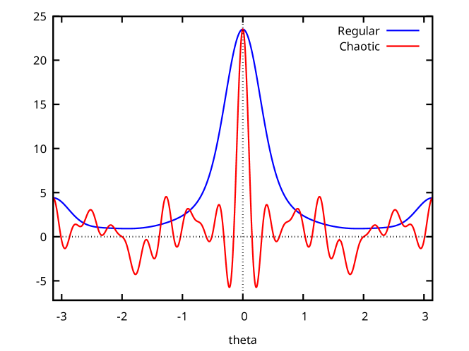
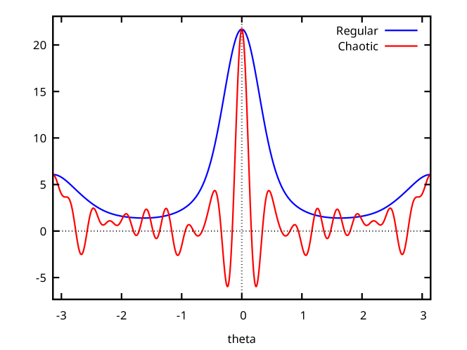
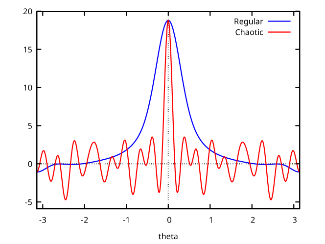
Figure 1: Three graphs of the functions $C_{N}(\theta)$ and $R_{N}(\theta)$ with highest frequency $N=20$

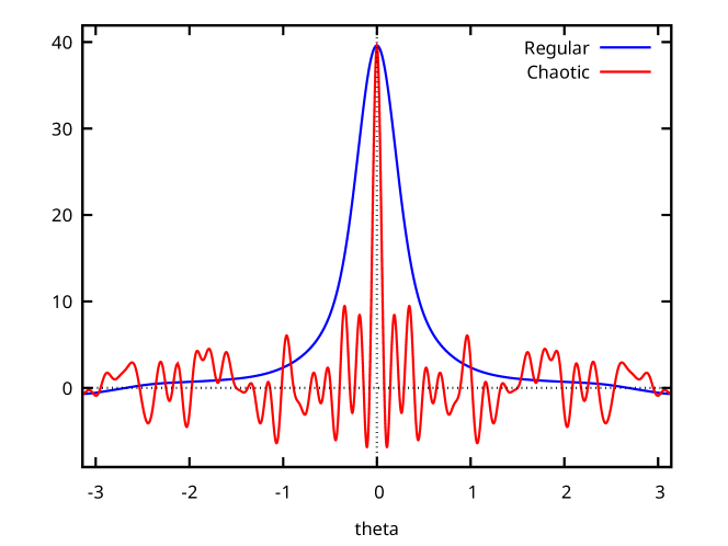
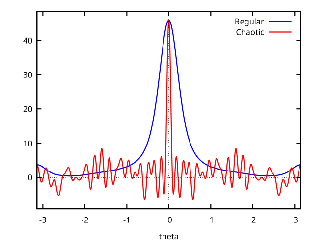
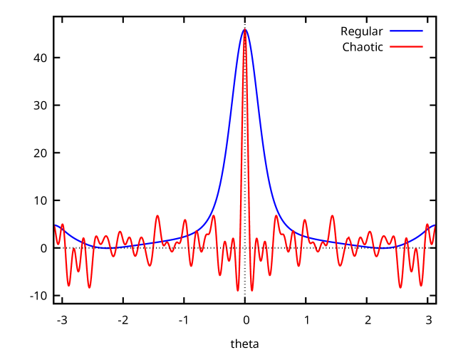
Figure 2: Three graphs of the functions $C_{N}(\theta)$ and $R_{N}(\theta)$ with highest frequency $N=40$

The two completely different behavior are associated to the same sequence of identically and independent random uniform variable in the interval $[0,2]$. In fact suppose we draw $N+1$ random numbers $c_{k}$ ($0\leq k\leq N$) from a uniform distribution in the interval $[0,2]$. We can then define two different functions which at first sight should have a similar graph

$$C_{N}(\theta)= \sum_{k=0}^{N}\,c_{k}\cos(k\theta),$$

$$R_{N}(\theta)= \sum_{k=0}^{N}\,c_{k}\left(\cos(\theta)\right)^{k},$$ (2.1)

but in reality the first function $C_{N}(\theta)$ has a “chaotic” behavior while the second function $R_{N}(\theta)$ has a regular behavior.

The reason of the very different behaviors is due to the fact that $|\cos(\theta)|\leq 1$ and therefore the contribution from $\left(\cos(\theta)\right)^{k}$ for big $k$ is suppressed w.r.t. f.x. $\cos(\theta)$ and $1$.

The idea is that the “non trivial part” of 4pts string amplitudes is encoded in a polynomial $P_{N}(s,t)$ in Mandelstam variables $s$ and $t$. At fixed center of mass energy $s$ the angular dependence is contained in $t\sim cos(\theta)$. Hence almost all angular dependence besides the one in Veneziano amplitude is in form of a polynomial $\hat{P}_{N}(s,cos(\theta))$. If we suppose that all coefficients in $P_{N}(s,t)$ are of the same order of magnitude then almost all interesting angular dependence is in the low $k$ terms, roughly $\cos(2\theta)$, $\cos(\theta)$ and $1$ because $|\cos(\theta)|\leq 1$.

We have written only $1$, $\cos(\theta)$ and $\cos(2\theta)$ because we can expect that higher $k$s dominate when all lower $k$ term vanish. But only $\cos(2^{m}\theta)$ ($m\in\mathbb{N}$) have no common zeros therefore generically $1$, $\cos(\theta)$ and $\cos(2\theta)$ will determine the behavior since their coefficients are also bigger for $R_{N}$ when written as a $\cos(k\theta)$ series.

We can make this statement more rigorous. If we rewrite $C_{N}(\theta)$ using $\cos(k\theta)$ we get

$$\hat{c}_{2m}= \sum_{l=0}^{[N/2]-m}{2l+2m\choose l}\frac{1}{2^{k+l}}2c_{2l+2m},$$

$$\hat{c}_{2m+1}= \sum_{l=0}^{[N/2]-m}{2l+2m+1\choose l}\frac{1}{2^{2l+2m}}c_{2l+2m+1}.$$ (2.2)

We can then compute their expectation values under the hypothesis that $c_{k}$ are independent and identically distributed random variables. We easily get

$$E[\hat{c}_{2m}]= 2\mu\sum_{l=0}^{[N/2]-m}{2l+2m\choose l}\frac{1}{2^{k+l}},$$

$$E[\hat{c}_{2m+1}]= \mu\,\sum_{l=0}^{[N/2]-m}{2l+2m+1\choose l}\frac{1}{2^{2l+2m}},$$ (2.3)

where $\mu=E[c_{k}]$ which is assumed to be different from zero since we can expect that the mean of the amplitudes be different from zero. A quick numerical evaluation shows that they are decreasing as $m$ increases.

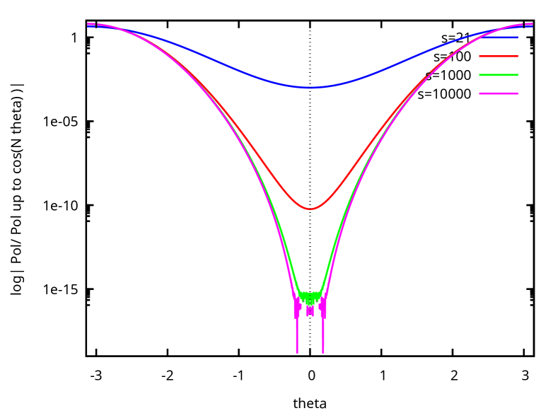
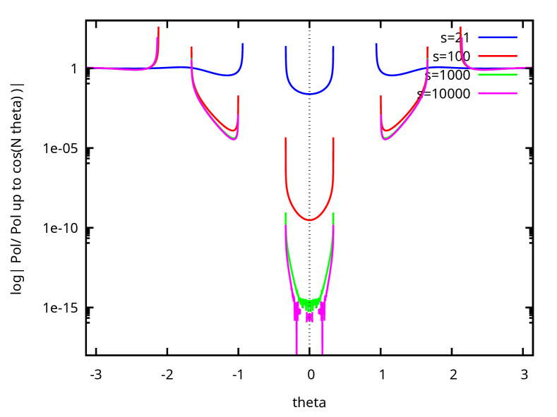
Figure 9: The graphs of $Pol(s,\cos(\theta))/Pol_{0}(s)$ and $Pol(s,\cos(\theta))/Pol_{4}(s)$ where $Pol_{N}(s)$ is $Pol(s,\cos(\theta))$ truncated to $\cos\left(N\theta\right)$ for different values of $s$ for the amplitude $S10z1S10z1TT$.

In section 4 on amplitudes we plot $\hat{P}_{N}(s,\cos(\theta))/\hat{P}_{N,M}(s,\cos(\theta))$ where $\hat{P}_{N,M}(s,\cos(\theta))$ is $\hat{P}_{N}(s,\cos(\theta))$ truncated to $\cos(M\theta)$. This is done for “small” and “big” values of $s$ and for $M=0$ and $M=4$ in figs. 3, 5, 7, 9 and 11 and find that the ratio is always of the order $1$ up to very few points as we could expect from the very naive hypothesis.

3 Massive scalar states and $\Pi$ gauge

In this section we would like to describe how we build the massive scalars we are going to use and the ambiguities related to the existence of null (BRST exact) states. The explicit computation shows explicitly what is known from theory: the degeneration of scalars at a given arbitrary level is independent on the space time dimension but the number of null states does depend on it.

We then describe how all is simplified in the $\Pi$ gauge. The gauge is also all very well suited to show explicitly that the degeneration of a given arbitrary spin at a given arbitrary level is independent on the spacetime dimension and on the existence of null states. What depends on spacetime dimension is the dimension of the irrep.

3.1 Building explicit representatives of scalar states

In order to describe the straightforward and simplest approach we use we start with the lightest massive scalar, the one at level $N=4$.

We first compute the scalar basis at level $N=4$. Differently from the lightcone we need to include also the zero modes $\alpha^{\mu}_{0}$ this makes the dimension of the vector space bigger. The explicit basis reads

$$\Big{\{} \left(1,0\right)^{4},\left(1,0\right)^{2}\,\left(1,1\right),\left(1,1\right)^{2},\left(1,0\right)^{2}\,\left(2,0\right),\left(1,1\right)\,\left(2,0\right),\left(2,0\right)^{2},$$

$$\left(1,0\right)\,\left(2,1\right),\left(2,2\right),\left(1,0\right)\,\left(3,0\right),\left(3,1\right),\left(4,0\right)\Big{\}},$$ (3.1)

where we use the short hand notation

$$(m,n)\equiv\alpha^{\mu}_{-m}\alpha^{\mu}_{-n},$$ (3.2)

and we do not explicitly write the momentum $|k_{\nu}\rangle$. This means f.x. that

$$\left(1,1\right)\,\left(2,0\right)\equiv\alpha_{-1}^{\mu}\alpha_{-1}^{\mu}\,\alpha_{-2}^{\nu}\alpha_{0}^{\nu}\,|k_{\rho}\rangle.$$ (3.3)

This basis has $11$ elements while the lightcone and $\Pi$ gauge basis have only $3$ elements, i.e. the previous elements without any $\alpha_{0}$. Explicitly

$$\Big{\{}\left(1,1\right)^{2},\left(2,2\right),\left(3,1\right)\Big{\}}.$$ (3.4)

Conceptually this is not a big difference but computationally it is since the computation of amplitudes requires by far more terms. For example the 3pts amplitude requires in principle without considering permutation symmetries $11^{3}$ sub-amplitudes in the straightforward computation versus $3^{3}$ sub-amplitudes in lightcone or $\Pi$ gauge.

The difference becomes quickly very big as the following table shows

$$\setcounter{MaxMatrixCols}{13}\begin{matrix}\backslash N&1&2&3&4&5&6&7&8&9&10&11&12\\ \mbox{cov}&1&3&5&11&18&35&57&102&165&279&444&726\\ \Pi\mbox{ gauge}&1&1&1&3&3&7&8&16&20&35&46&77\end{matrix}.$$ (3.5)

After we have construct the basis we can consider the most general scalar state as a linear combination of the basis elements

$$|SC_{4}\rangle= \left(4,0\right)\,s_{11}+\left(3,1\right)\,s_{10}+\left(1,0\right)\,\left(3,0\right)\,s_{9}+\left(2,2\right)\,s_{8}$$

$$+\left(1,0\right)\,\left(2,1\right)\,s_{7}+\left(2,0\right)^{2}\,s_{6}+\left(1,1\right)\,\left(2,0\right)\,s_{5}$$

$$+\left(1,0\right)^{2}\,\left(2,0\right)\,s_{4}+\left(1,1\right)^{2}\,s_{3}+\left(1,0\right)^{2}\,\left(1,1\right)\,s_{2}+\left(1,0\right)^{4}\,s_{1},$$ (3.6)

and then require it a primary field by imposing

$$L_{1}|SC_{4}\rangle=L_{2}|SC_{4}\rangle=0.$$ (3.7)

This gives $3$ independent (but not orthogonal) solutions, i.e

$$|s_{4\,1}\rangle= -{{2\,(2{\alpha^{\prime}}k^{2})^{2}\,\left(D+1\right)}\over{3}}\,\left(3,1\right)+{{2\,(2{\alpha^{\prime}}k^{2})\,\left(D+1\right)}\over{3}}\,\left(1,0\right)\,\left(3,0\right)+{{(2{\alpha^{\prime}}k^{2})^{2}\,\left(D+1\right)}\over{2}}\,\left(2,2\right)$$

$$-{{(2{\alpha^{\prime}}k^{2})\,\left(D+1\right)}\over{2}}\,\left(2,0\right)^{2}+(2{\alpha^{\prime}}k^{2})^{2}\,\left(1,1\right)^{2}-2\,\left(0,0\right)\,\left(1,0\right)^{2}\,\left(1,1\right)+\left(1,0\right)^{4}$$ (3.8)

$$|s_{4\,2}\rangle= -{{\left(4\,D^{2}-2\,(2{\alpha^{\prime}}k^{2})\,D+21\,D-2\,(2{\alpha^{\prime}}k^{2})^{2}+(2{\alpha^{\prime}}k^{2})+20\right)}\over{4\,(2{\alpha^{\prime}}k^{2})\,\left(2\,(2{\alpha^{\prime}}k^{2})-9\right)}}\left(2,0\right)^{2}$$

$$+{{\left(4\,D^{2}-4\,(2{\alpha^{\prime}}k^{2})\,D+18\,D-2\,(2{\alpha^{\prime}}k^{2})^{2}+3\,(2{\alpha^{\prime}}k^{2})+23\right)}\over{4\,\left(2\,(2{\alpha^{\prime}}k^{2})-9\right)}}\left(2,2\right)$$

$$-{{\left(4\,D^{2}-4\,(2{\alpha^{\prime}}k^{2})\,D+18\,D-6\,(2{\alpha^{\prime}}k^{2})+23\right)}\over{3\,\left(2\,(2{\alpha^{\prime}}k^{2})-9\right)}}\left(3,1\right)$$

$$+{{\left(4\,D^{2}-10\,(2{\alpha^{\prime}}k^{2})\,D+21\,D+20\right)}\over{3\,(2{\alpha^{\prime}}k^{2})\,\left(2\,(2{\alpha^{\prime}}k^{2})-9\right)}}\left(1,0\right)\,\left(3,0\right)+{{\left(4\,D-2\,(2{\alpha^{\prime}}k^{2})+5\right)}\over{(2{\alpha^{\prime}}k^{2})\,\left(2\,(2{\alpha^{\prime}}k^{2})-9\right)}}\left(1,0\right)^{2}\,\left(2,0\right)$$

$$-{{\left(4\,D-2\,(2{\alpha^{\prime}}k^{2})+5\right)}\over{(2{\alpha^{\prime}}k^{2})\,\left(2\,(2{\alpha^{\prime}}k^{2})-9\right)}}\left(1,0\right)^{2}\,\left(1,1\right)+{{\left(2\,D-2\,(2{\alpha^{\prime}}k^{2})+7\right)}\over{2\,(2{\alpha^{\prime}}k^{2})-9}}\left(1,1\right)^{2}\,$$

$$+{{\left(2\,(2{\alpha^{\prime}}k^{2})-1\right)\,\left(D-1\right)}\over{4\,\left(2\,(2{\alpha^{\prime}}k^{2})-9\right)}}\,\left(4,0\right)+\left(1,0\right)\,\left(2,1\right)$$ (3.9)

$$|s_{4\,3}\rangle= -{{\left(D^{2}-2\,(2{\alpha^{\prime}}k^{2})\,D+12\,D+4\,(2{\alpha^{\prime}}k^{2})^{2}-26\,(2{\alpha^{\prime}}k^{2})+32\right)}\over{4\,(2{\alpha^{\prime}}k^{2})\,\left(2\,(2{\alpha^{\prime}}k^{2})-9\right)}}\left(2,0\right)^{2}\,$$

$$-{{\left(D^{2}-4\,(2{\alpha^{\prime}}k^{2})\,D+18\,D+4\,(2{\alpha^{\prime}}k^{2})^{2}-24\,(2{\alpha^{\prime}}k^{2})+26\right)}\over{3\,\left(2\,(2{\alpha^{\prime}}k^{2})-9\right)}}\left(3,1\right)\,$$

$$+{{\left(D^{2}-4\,(2{\alpha^{\prime}}k^{2})\,D+18\,D+4\,(2{\alpha^{\prime}}k^{2})^{2}-24\,(2{\alpha^{\prime}}k^{2})+26\right)}\over{4\,\left(2\,(2{\alpha^{\prime}}k^{2})-9\right)}}\left(2,2\right)\,$$

$$+{{\left(D-2\,(2{\alpha^{\prime}}k^{2})+4\right)\,\left(D-2\,(2{\alpha^{\prime}}k^{2})+8\right)}\over{3\,(2{\alpha^{\prime}}k^{2})\,\left(2\,(2{\alpha^{\prime}}k^{2})-9\right)}}\left(1,0\right)\,\left(3,0\right)\,+{{\left(D-2\,(2{\alpha^{\prime}}k^{2})+8\right)}\over{(2{\alpha^{\prime}}k^{2})\,\left(2\,(2{\alpha^{\prime}}k^{2})-9\right)}}\left(1,0\right)^{2}\,\left(2,0\right)\,$$

$$-{{\left(D-2\,(2{\alpha^{\prime}}k^{2})+8\right)}\over{(2{\alpha^{\prime}}k^{2})\,\left(2\,(2{\alpha^{\prime}}k^{2})-9\right)}}\left(1,0\right)^{2}\,\left(1,1\right)\,+{{\left(D-4\,(2{\alpha^{\prime}}k^{2})+17\right)}\over{2\,\left(2\,(2{\alpha^{\prime}}k^{2})-9\right)}}\left(1,1\right)^{2}\,$$

$$+{{\left(D-1\right)}\over{2\,\left(2\,(2{\alpha^{\prime}}k^{2})-9\right)}}\left(4,0\right)\,+\left(1,1\right)\,\left(2,0\right).$$ (3.10)

In the previous expression $D$ is the spacetime dimension. The number of solutions does not depend of $D$ or the mass shell condition.

On the other side we know that there is only one scalar at level $N=4$ therefore all the previous states must be describe the same physical scalar. There is also the possibility that some of them are null (BRST exact) states.

To exactly count the physical scalars at this level we have to find the null states. This requires to find a basis for scalar states at level $N-1=3$

$$\left\{\left(1,0\right)^{3},\left(1,0\right)\,\left(1,1\right),\left(1,0\right)\,\left(2,0\right),\left(2,1\right),\left(3,0\right)\right\},$$ (3.11)

and at level $N-2=2$

$$\left\{\left(1,0\right)^{2},\left(1,1\right),\left(2,0\right)\right\},$$ (3.12)

then to make the general linear superposition and then build their images under $L_{-1}$ and $L_{-2}$ respectively. The result of the previous steps is a scalar state at level $N=4$ which is not necessarily associated with a primary field, i.e. physical. We get

$$= 2\,\left(4,0\right)\,n_{8}+\left(2,0\right)^{2}\,n_{8}+{{\left(1,1\right)\,\left(2,0\right)\,n_{8}}\over{2}}$$

$$+2\,\left(3,1\right)\,n_{7}+\left(1,1\right)\,\left(2,0\right)\,n_{7}+{{\left(1,1\right)^{2}\,n_{7}}\over{2}}$$

$$+2\,\left(1,0\right)\,\left(3,0\right)\,n_{6}+\left(1,0\right)^{2}\,\left(2,0\right)\,n_{6}+{{\left(1,0\right)^{2}\,\left(1,1\right)\,n_{6}}\over{2}}$$

$$+3\,\left(4,0\right)\,n_{5}+\left(1,0\right)\,\left(3,0\right)\,n_{5}$$

$$+2\,\left(3,1\right)\,n_{4}+\left(2,2\right)\,n_{4}+\left(1,0\right)\,\left(2,1\right)\,n_{4}$$

$$+2\,\left(1,0\right)\,n_{3}\,\left(3,0\right)+\left(2,0\right)^{2}\,n_{3}+\left(1,0\right)^{2}\,\left(2,0\right)\,n_{3}$$

$$+2\,\left(1,0\right)\,n_{2}\,\left(2,1\right)+\left(1,1\right)\,n_{2}\,\left(2,0\right)+\left(1,0\right)^{2}\,\left(1,1\right)\,n_{2}$$

$$+3\,n_{1}\,\left(1,0\right)^{2}\,\left(2,0\right)+n_{1}\,\left(1,0\right)^{4}.$$ (3.13)

This expression has $8=5+3$ undetermined coefficients as many as the dimension of the scalar basis used to build it.

In critical dimension $D=26$ and on mass shell $(0,0)=(2{\alpha^{\prime}}k^{2})=-2(4-1)=-6$ only we get $2$ null states.

These null states may be used to simplify the physical level $4$ scalar $r_{1}|s_{4\,1}\rangle+r_{2}|s_{4\,2}\rangle+r_{3}|s_{4\,3}\rangle$. There is no unique way. One possible gauge is to try to set to zero the terms with the highest number of zero modes $\alpha^{\mu}_{0}$. The result is reported in section 3.3 which contains the states we actually used to perform the computations.

There are also other possibilities. For example to try to set to zero the coefficients of the terms with the highest excitation $m$ $\alpha^{\mu}_{-m}$.

Actually there is a very efficient gauge which we describe now.

3.2 Scalar and massive states in $\Pi$ gauge

In the previous subsection we have seen that building explicitly scalar (and massive) states in covariant formalism may be computationally more demanding than build them in lightcone as done in [51]. This happens because the covariant basis are bigger. We want now to show that there exists a very effective and conceptually illuminating gauge which we dub $\Pi$ gauge.

The idea is very simple. In [22] it was noticed that replacing the usual polarizations with the projected polarizations as

$$\epsilon_{\mu}\leavevmode\nobreak\ \leavevmode\nobreak\ \rightarrow\leavevmode\nobreak\ \leavevmode\nobreak\ (\Pi\epsilon)_{\mu}=\left(\delta_{\mu}^{\nu}-\frac{k_{\mu}k^{\nu}}{k^{2}}\right)\epsilon_{\nu},$$ (3.14)

led to a simplification in the conditions imposed by Virasoro constraints. Now we further generalize this approach and we build the scalar basis (and all the other states) using the projector $\Pi_{\mu}^{.\,\nu}(\alpha_{0})=\left(\delta_{\mu}^{\nu}-\frac{\alpha_{0\,\mu}\alpha_{0}^{\nu}}{(\alpha_{0})^{2}}\right)$ using

$$[m,n]=(m,n)_{\Pi}\equiv\alpha^{\mu}_{-m}\,\Pi_{\mu\nu}(\alpha_{0})\,\alpha^{\nu}_{-n}.$$ (3.15)

This immediately leads to the collapse of the size of the covariant basis to the same size of the lightcone one, i.e for $N=4$ scalars

$$\Big{\{}\left[1,1\right]^{2},\left[2,2\right],\left[3,1\right]\Big{\}}.$$ (3.16)

The obvious and natural question is whether this is not too restrictive and whether we can describe all physical states in this way. The answer is that it is possible and this a very efficient way since it eliminates completely the necessity of considering null states. The reason is very simple. If we describe the massive state in the rest frame, also when it is off shell as long as $E\neq 0$, then the projector eliminates all the objects with a temporal index $\mu=0$ since $\Pi_{\mu=0}^{.\,\nu}\Big{|}_{rest}=\Pi_{\mu}^{.\,\nu=0}\Big{|}_{rest}=0$. This means that all states build using the previous basis have positive norm. This is the crucial point since any null state has by definition a null norm hence it must contain in some way some $\alpha^{\mu=0}$. It follows that we can forget about null states since their action moves any state out of the $\Pi$ gauge. This in turn means that the “gauge orbit” of a physical state generated by the null states must have a representative in the $\Pi$ gauge. Even more, because of the discussion on the previous section which rephrases the classical knowledge that only the number of null states does depend on the dimension of spacetime and on shell condition we see that the degeneration of a physical (also off shell) states for a given spin and for a given mass level is independent on the spacetime dimension. This construction makes very concrete the same assertion made in [52, 53, 54] which was based on computing the degenerations by using characters.

The level $N=4$ scalar state reads in this gauge

$$-{{2\,\left(D_{eff}+2\right)}\over{3}}\left[3,1\right]\,+{{\left(D_{eff}+2\right)}\over{2}}\left[2,2\right]\,+\left[1,1\right]^{2},$$ (3.17)

where $D_{eff}=D-1$.

3.3 The states used

The states we used in the actual computations are the following.

The level $4$ scalar with the maximum number of terms the highest occurrences of zero modes eliminated using the null states which has $8$ terms out of $11$ possible reads

$$|S4z\rangle= 1500\,\left(4,0\right)-7104\,\left(3,1\right)-184\,\left(1,0\right)\,\left(3,0\right)+5742\,\left(2,2\right)+276\,\left(1,0\right)\,\left(2,1\right)$$

$$+432\,\left(2,0\right)^{2}-726\,\left(1,1\right)\,\left(2,0\right)+225\,\left(1,1\right)^{2},$$ (3.18)

The level $6$ scalar with the maximum number of terms the highest occurrences of zero modes eliminated using the null states which has $22$ terms out of $35$ possible reads

$$|S6z\rangle= -226500\,\left(6,0\right)+1177320\,\left(5,1\right)-18168\,\left(1,0\right)\,\left(5,0\right)$$

$$-1872750\,\left(4,2\right)+214110\,\left(1,0\right)\,\left(4,1\right)-141150\,\left(2,0\right)\,\left(4,0\right)$$

$$+79515\,\left(1,1\right)\,\left(4,0\right)+929500\,\left(3,3\right)-191400\,\left(1,0\right)\,\left(3,2\right)$$

$$+100680\,\left(2,0\right)\,\left(3,1\right)-337500\,\left(1,1\right)\,\left(3,1\right)+75700\,\left(3,0\right)^{2}$$

$$+9720\,\left(2,1\right)\,\left(3,0\right)-43875\,\left(2,0\right)\,\left(2,2\right)+251225\,\left(1,1\right)\,\left(2,2\right)$$

$$-7975\,\left(1,0\right)^{2}\,\left(2,2\right)+1900\,\left(2,1\right)^{2}+15950\,\left(1,0\right)\,\left(2,0\right)\,\left(2,1\right)$$

$$-6750\,\left(2,0\right)^{3}+12275\,\left(1,1\right)\,\left(2,0\right)^{2}-20250\,\left(1,1\right)^{2}\,\left(2,0\right)+6750\,\left(1,1\right)^{3},$$ (3.19)

The first level $8$ scalar with the maximum number of terms the highest occurrences of zero modes eliminated using the null states has $65$ terms out of $102$ possible and reads

$$|S8z1\rangle= -54920250\,\left(8,0\right)+419373360\,\left(7,1\right)-1427760\,\left(1,0\right)\,\left(7,0\right)$$

$$-2262735720\,\left(6,2\right)-113561280\,\left(1,0\right)\,\left(6,1\right)-64299480\,\left(2,0\right)\,\left(6,0\right)$$

$$+126077280\,\left(1,1\right)\,\left(6,0\right)+6188984592\,\left(5,3\right)+356467104\,\left(1,0\right)\,\left(5,2\right)$$

$$+384247584\,\left(2,0\right)\,\left(5,1\right)-383096448\,\left(1,1\right)\,\left(5,1\right)+1209600\,\left(1,0\right)^{2}\,\left(5,1\right)$$

$$+135449328\,\left(3,0\right)\,\left(5,0\right)-262211040\,\left(2,1\right)\,\left(5,0\right)+10184832\,\left(1,0\right)\,\left(2,0\right)\,\left(5,0\right)$$

$$-10789632\,\left(1,0\right)\,\left(1,1\right)\,\left(5,0\right)-4300632000\,\left(4,4\right)-247152360\,\left(1,0\right)\,\left(4,3\right)$$

$$-1212819300\,\left(2,0\right)\,\left(4,2\right)+512024310\,\left(1,1\right)\,\left(4,2\right)-12882555\,\left(1,0\right)^{2}\,\left(4,2\right)$$

$$-18257400\,\left(3,0\right)\,\left(4,1\right)+529542090\,\left(2,1\right)\,\left(4,1\right)-2116485\,\left(1,0\right)\,\left(2,0\right)\,\left(4,1\right)$$

$$+11975040\,\left(1,0\right)\,\left(1,1\right)\,\left(4,1\right)-73024875\,\left(4,0\right)^{2}-222613440\,\left(3,1\right)\,\left(4,0\right)$$

$$-10558800\,\left(1,0\right)\,\left(3,0\right)\,\left(4,0\right)+462861000\,\left(2,2\right)\,\left(4,0\right)+28720755\,\left(1,0\right)\,\left(2,1\right)\,\left(4,0\right)$$

$$-19570950\,\left(2,0\right)^{2}\,\left(4,0\right)+16215885\,\left(1,1\right)\,\left(2,0\right)\,\left(4,0\right)-11975040\,\left(1,1\right)^{2}\,\left(4,0\right)$$

$$+910342720\,\left(2,0\right)\,\left(3,3\right)-223149500\,\left(1,1\right)\,\left(3,3\right)+13777750\,\left(1,0\right)^{2}\,\left(3,3\right)$$

$$-156750720\,\left(3,0\right)\,\left(3,2\right)-360009720\,\left(2,1\right)\,\left(3,2\right)-15677340\,\left(1,0\right)\,\left(2,0\right)\,\left(3,2\right)$$

$$-772800\,\left(1,0\right)\,\left(1,1\right)\,\left(3,2\right)-42000\,\left(1,0\right)^{3}\,\left(3,2\right)+539448700\,\left(3,1\right)^{2}$$

$$-14149100\,\left(1,0\right)\,\left(3,0\right)\,\left(3,1\right)-1237619880\,\left(2,2\right)\,\left(3,1\right)-22545600\,\left(1,0\right)\,\left(2,1\right)\,\left(3,1\right)$$

$$+26813220\,\left(2,0\right)^{2}\,\left(3,1\right)-631680\,\left(1,1\right)\,\left(2,0\right)\,\left(3,1\right)+42000\,\left(1,0\right)^{2}\,\left(2,0\right)\,\left(3,1\right)$$

$$+20048000\,\left(2,0\right)\,\left(3,0\right)^{2}+8144150\,\left(1,1\right)\,\left(3,0\right)^{2}+10255140\,\left(1,0\right)\,\left(2,2\right)\,\left(3,0\right)$$

$$-68817420\,\left(2,0\right)\,\left(2,1\right)\,\left(3,0\right)+23950080\,\left(1,1\right)\,\left(2,1\right)\,\left(3,0\right)+42000\,\left(1,0\right)^{2}\,\left(2,1\right)\,\left(3,0\right)$$

$$-42000\,\left(1,0\right)\,\left(1,1\right)\,\left(2,0\right)\,\left(3,0\right)+618823800\,\left(2,2\right)^{2}+11264400\,\left(1,0\right)\,\left(2,1\right)\,\left(2,2\right)$$

$$+19192950\,\left(2,0\right)^{2}\,\left(2,2\right)-35002800\,\left(1,1\right)\,\left(2,0\right)\,\left(2,2\right)+63000\,\left(1,0\right)^{2}\,\left(2,0\right)\,\left(2,2\right)$$

$$+12448800\,\left(1,1\right)^{2}\,\left(2,2\right)+23738400\,\left(2,0\right)\,\left(2,1\right)^{2}-12448800\,\left(1,1\right)\,\left(2,1\right)^{2}$$

$$-126000\,\left(1,0\right)\,\left(2,0\right)^{2}\,\left(2,1\right)+63000\,\left(1,1\right)\,\left(2,0\right)^{3},$$ (3.20)

The second level $8$ scalar with the maximum number of terms the highest occurrences of zero modes has again $65$ terms out of $102$ possible and reads

$$|S8z2\rangle= -46478250\,\left(8,0\right)+359941680\,\left(7,1\right)-848880\,\left(1,0\right)\,\left(7,0\right)$$

$$-1931385960\,\left(6,2\right)-95941440\,\left(1,0\right)\,\left(6,1\right)-55667640\,\left(2,0\right)\,\left(6,0\right)$$

$$106609440\,\left(1,1\right)\,\left(6,0\right)+5264441616\,\left(5,3\right)+300357792\,\left(1,0\right)\,\left(5,2\right)$$

$$+324832032\,\left(2,0\right)\,\left(5,1\right)-328898304\,\left(1,1\right)\,\left(5,1\right)+604800\,\left(1,0\right)^{2}\,\left(5,1\right)$$

$$+118298544\,\left(3,0\right)\,\left(5,0\right)-220237920\,\left(2,1\right)\,\left(5,0\right)+8963136\,\left(1,0\right)\,\left(2,0\right)\,\left(5,0\right)$$

$$-9265536\,\left(1,0\right)\,\left(1,1\right)\,\left(5,0\right)-3654567000\,\left(4,4\right)-208166280\,\left(1,0\right)\,\left(4,3\right)$$

$$-1028682900\,\left(2,0\right)\,\left(4,2\right)+439123230\,\left(1,1\right)\,\left(4,2\right)-10779615\,\left(1,0\right)^{2}\,\left(4,2\right)$$

$$-10546200\,\left(3,0\right)\,\left(4,1\right)+453611970\,\left(2,1\right)\,\left(4,1\right)-802305\,\left(1,0\right)\,\left(2,0\right)\,\left(4,1\right)$$

$$10069920\,\left(1,0\right)\,\left(1,1\right)\,\left(4,1\right)-64519875\,\left(4,0\right)^{2}-194265120\,\left(3,1\right)\,\left(4,0\right)$$

$$-9248400\,\left(1,0\right)\,\left(3,0\right)\,\left(4,0\right)+393876000\,\left(2,2\right)\,\left(4,0\right)+24652215\,\left(1,0\right)\,\left(2,1\right)\,\left(4,0\right)$$

$$-17038350\,\left(2,0\right)^{2}\,\left(4,0\right)+13616505\,\left(1,1\right)\,\left(2,0\right)\,\left(4,0\right)-10069920\,\left(1,1\right)^{2}\,\left(4,0\right)$$

$$772506560\,\left(2,0\right)\,\left(3,3\right)-191999500\,\left(1,1\right)\,\left(3,3\right)+11726750\,\left(1,0\right)^{2}\,\left(3,3\right)$$

$$-134722560\,\left(3,0\right)\,\left(3,2\right)-305834760\,\left(2,1\right)\,\left(3,2\right)-13549620\,\left(1,0\right)\,\left(2,0\right)\,\left(3,2\right)$$

$$-512400\,\left(1,0\right)\,\left(1,1\right)\,\left(3,2\right)-21000\,\left(1,0\right)^{3}\,\left(3,2\right)+464137100\,\left(3,1\right)^{2}$$

$$-11458300\,\left(1,0\right)\,\left(3,0\right)\,\left(3,1\right)-1064138040\,\left(2,2\right)\,\left(3,1\right)-19210800\,\left(1,0\right)\,\left(2,1\right)\,\left(3,1\right)$$

$$+21328860\,\left(2,0\right)^{2}\,\left(3,1\right)-416640\,\left(1,1\right)\,\left(2,0\right)\,\left(3,1\right)+21000\,\left(1,0\right)^{2}\,\left(2,0\right)\,\left(3,1\right)$$

$$+17416000\,\left(2,0\right)\,\left(3,0\right)^{2}+6809950\,\left(1,1\right)\,\left(3,0\right)^{2}+7657020\,\left(1,0\right)\,\left(2,2\right)\,\left(3,0\right)$$

$$-57671460\,\left(2,0\right)\,\left(2,1\right)\,\left(3,0\right)+20139840\,\left(1,1\right)\,\left(2,1\right)\,\left(3,0\right)+21000\,\left(1,0\right)^{2}\,\left(2,1\right)\,\left(3,0\right)$$

$$-21000\,\left(1,0\right)\,\left(1,1\right)\,\left(2,0\right)\,\left(3,0\right)+530541900\,\left(2,2\right)^{2}+9601200\,\left(1,0\right)\,\left(2,1\right)\,\left(2,2\right)$$

$$+17038350\,\left(2,0\right)^{2}\,\left(2,2\right)-30038400\,\left(1,1\right)\,\left(2,0\right)\,\left(2,2\right)+10823400\,\left(1,1\right)^{2}\,\left(2,2\right)$$

$$+31500\,\left(1,0\right)^{2}\,\left(1,1\right)\,\left(2,2\right)+20437200\,\left(2,0\right)\,\left(2,1\right)^{2}-10823400\,\left(1,1\right)\,\left(2,1\right)^{2}$$

$$-63000\,\left(1,0\right)\,\left(1,1\right)\,\left(2,0\right)\,\left(2,1\right)+31500\,\left(1,1\right)^{2}\,\left(2,0\right)^{2},$$ (3.21)

The first level $10$ scalar with the maximum number of terms the highest occurrences of zero modes eliminated using the null states has $157$ terms out of $279$ possible and reads

$$|S10z1\rangle= -6935292000\,\left(10,0\right)+94471732800\,\left(9,1\right)+1395489600\,\left(1,0\right)\,\left(9,0\right)$$

$$-456913920600\,\left(8,2\right)-3532347000\,\left(1,0\right)\,\left(8,1\right)-15851576700\,\left(2,0\right)\,\left(8,0\right)$$

$$+16188732000\,\left(1,1\right)\,\left(8,0\right)+269482500\,\left(1,0\right)^{2}\,\left(8,0\right)+1017474393600\,\left(7,3\right)$$

$$-33493788000\,\left(1,0\right)\,\left(7,2\right)+68103216000\,\left(2,0\right)\,\left(7,1\right)-52980480000\,\left(1,1\right)\,\left(7,1\right)$$

$$-1805580000\,\left(1,0\right)^{2}\,\left(7,1\right)+25637875200\,\left(3,0\right)\,\left(7,0\right)-32628708000\,\left(2,1\right)\,\left(7,0\right)$$

$$-801360000\,\left(1,0\right)\,\left(2,0\right)\,\left(7,0\right)+626220000\,\left(1,0\right)\,\left(1,1\right)\,\left(7,0\right)-1256174740800\,\left(6,4\right)$$

$$+116534544000\,\left(1,0\right)\,\left(6,3\right)-116617158000\,\left(2,0\right)\,\left(6,2\right)+177150240000\,\left(1,1\right)\,\left(6,2\right)$$

$$+6561480000\,\left(1,0\right)^{2}\,\left(6,2\right)-71086512000\,\left(3,0\right)\,\left(6,1\right)-6006960000\,\left(2,1\right)\,\left(6,1\right)$$

$$+1345650000\,\left(1,0\right)\,\left(2,0\right)\,\left(6,1\right)-1587600000\,\left(1,0\right)\,\left(1,1\right)\,\left(6,1\right)+11300654400\,\left(4,0\right)\,\left(6,0\right)$$

$$-255510192000\,\left(3,1\right)\,\left(6,0\right)-5662720000\,\left(1,0\right)\,\left(3,0\right)\,\left(6,0\right)+254080638000\,\left(2,2\right)\,\left(6,0\right)$$

$$+854670000\,\left(1,0\right)\,\left(2,1\right)\,\left(6,0\right)+7813260000\,\left(2,0\right)^{2}\,\left(6,0\right)-5427840000\,\left(1,1\right)\,\left(2,0\right)\,\left(6,0\right)$$

$$+1587600000\,\left(1,1\right)^{2}\,\left(6,0\right)+607282147584\,\left(5,5\right)-81345942720\,\left(1,0\right)\,\left(5,4\right)$$

$$+2634992640\,\left(2,0\right)\,\left(5,3\right)-551036203200\,\left(1,1\right)\,\left(5,3\right)-20082748000\,\left(1,0\right)^{2}\,\left(5,3\right)$$

$$+225351473760\,\left(3,0\right)\,\left(5,2\right)+247693312800\,\left(2,1\right)\,\left(5,2\right)+12886098000\,\left(1,0\right)\,\left(2,0\right)\,\left(5,2\right)$$

$$-5267808000\,\left(1,0\right)\,\left(1,1\right)\,\left(5,2\right)-104496000\,\left(1,0\right)^{3}\,\left(5,2\right)-89828383680\,\left(4,0\right)\,\left(5,1\right)$$

$$+865169323200\,\left(3,1\right)\,\left(5,1\right)+29446648000\,\left(1,0\right)\,\left(3,0\right)\,\left(5,1\right)-790017472800\,\left(2,2\right)\,\left(5,1\right)$$

$$-5845392000\,\left(1,0\right)\,\left(2,1\right)\,\left(5,1\right)-36082698000\,\left(2,0\right)^{2}\,\left(5,1\right)+15876000000\,\left(1,1\right)\,\left(2,0\right)\,\left(5,1\right)$$

$$+104496000\,\left(1,0\right)^{2}\,\left(2,0\right)\,\left(5,1\right)-23408646912\,\left(5,0\right)^{2}+368756136000\,\left(4,1\right)\,\left(5,0\right)$$

$$+6258067200\,\left(1,0\right)\,\left(4,0\right)\,\left(5,0\right)-319433436000\,\left(3,2\right)\,\left(5,0\right)+9348102400\,\left(1,0\right)\,\left(3,1\right)\,\left(5,0\right)$$

$$-9549187200\,\left(2,0\right)\,\left(3,0\right)\,\left(5,0\right)-5376162400\,\left(1,1\right)\,\left(3,0\right)\,\left(5,0\right)-12435219600\,\left(1,0\right)\,\left(2,2\right)\,\left(5,0\right)$$

$$+17850699600\,\left(2,0\right)\,\left(2,1\right)\,\left(5,0\right)-4762800000\,\left(1,1\right)\,\left(2,1\right)\,\left(5,0\right)+104496000\,\left(1,0\right)^{2}\,\left(2,1\right)\,\left(5,0\right)$$

$$-104496000\,\left(1,0\right)\,\left(1,1\right)\,\left(2,0\right)\,\left(5,0\right)+59737860000\,\left(2,0\right)\,\left(4,4\right)+412610955750\,\left(1,1\right)\,\left(4,4\right)$$

$$+14943553275\,\left(1,0\right)^{2}\,\left(4,4\right)-167485920000\,\left(3,0\right)\,\left(4,3\right)-215509203000\,\left(2,1\right)\,\left(4,3\right)$$

$$-12604951100\,\left(1,0\right)\,\left(2,0\right)\,\left(4,3\right)+6371568000\,\left(1,0\right)\,\left(1,1\right)\,\left(4,3\right)+123480000\,\left(1,0\right)^{3}\,\left(4,3\right)$$

$$-286098435000\,\left(4,0\right)\,\left(4,2\right)-271032372000\,\left(3,1\right)\,\left(4,2\right)-43951472400\,\left(1,0\right)\,\left(3,0\right)\,\left(4,2\right)$$

$$+55566000000\,\left(2,2\right)\,\left(4,2\right)+61435500\,\left(1,0\right)\,\left(2,1\right)\,\left(4,2\right)+2976750000\,\left(2,0\right)^{2}\,\left(4,2\right)$$

$$+54671452500\,\left(1,1\right)\,\left(2,0\right)\,\left(4,2\right)+446460000\,\left(1,0\right)^{2}\,\left(2,0\right)\,\left(4,2\right)-28894320000\,\left(1,1\right)^{2}\,\left(4,2\right)$$

$$-370440000\,\left(1,0\right)^{2}\,\left(1,1\right)\,\left(4,2\right)-771289485750\,\left(4,1\right)^{2}-40007615550\,\left(1,0\right)\,\left(4,0\right)\,\left(4,1\right)$$

$$+1332626535000\,\left(3,2\right)\,\left(4,1\right)+15484392000\,\left(1,0\right)\,\left(3,1\right)\,\left(4,1\right)+73883607500\,\left(2,0\right)\,\left(3,0\right)\,\left(4,1\right)$$

$$-33498360000\,\left(1,1\right)\,\left(3,0\right)\,\left(4,1\right)-123480000\,\left(1,0\right)^{2}\,\left(3,0\right)\,\left(4,1\right)+8829124500\,\left(1,0\right)\,\left(2,2\right)\,\left(4,1\right)$$

$$-55227112500\,\left(2,0\right)\,\left(2,1\right)\,\left(4,1\right)+28894320000\,\left(1,1\right)\,\left(2,1\right)\,\left(4,1\right)-446460000\,\left(1,0\right)\,\left(2,0\right)^{2}\,\left(4,1\right)$$

$$+370440000\,\left(1,0\right)\,\left(1,1\right)\,\left(2,0\right)\,\left(4,1\right)-6952837500\,\left(2,0\right)\,\left(4,0\right)^{2}+11311477275\,\left(1,1\right)\,\left(4,0\right)^{2}$$

$$+347766720000\,\left(3,3\right)\,\left(4,0\right)+37648107500\,\left(1,0\right)\,\left(3,2\right)\,\left(4,0\right)-2610368400\,\left(2,0\right)\,\left(3,1\right)\,\left(4,0\right)$$

$$+11642400000\,\left(1,1\right)\,\left(3,1\right)\,\left(4,0\right)-123480000\,\left(1,0\right)^{2}\,\left(3,1\right)\,\left(4,0\right)+8643600000\,\left(3,0\right)^{2}\,\left(4,0\right)$$

$$-19766203100\,\left(2,1\right)\,\left(3,0\right)\,\left(4,0\right)+123480000\,\left(1,0\right)\,\left(1,1\right)\,\left(3,0\right)\,\left(4,0\right)-2976750000\,\left(2,0\right)\,\left(2,2\right)\,\left(4,0\right)$$

$$-23835724500\,\left(1,1\right)\,\left(2,2\right)\,\left(4,0\right)+165900000\,\left(1,0\right)^{2}\,\left(2,2\right)\,\left(4,0\right)+15500824500\,\left(2,1\right)^{2}\,\left(4,0\right)$$

$$-778260000\,\left(1,0\right)\,\left(2,0\right)\,\left(2,1\right)\,\left(4,0\right)+370440000\,\left(1,0\right)\,\left(1,1\right)\,\left(2,1\right)\,\left(4,0\right)+612360000\,\left(1,1\right)\,\left(2,0\right)^{2}\,\left(4,0\right)$$

$$-370440000\,\left(1,1\right)^{2}\,\left(2,0\right)\,\left(4,0\right)-414892800000\,\left(3,1\right)\,\left(3,3\right)+17012800000\,\left(1,0\right)\,\left(3,0\right)\,\left(3,3\right)$$

$$+556646958000\,\left(2,2\right)\,\left(3,3\right)+6659590000\,\left(1,0\right)\,\left(2,1\right)\,\left(3,3\right)+26403816600\,\left(2,0\right)^{2}\,\left(3,3\right)$$

$$-68300806000\,\left(1,1\right)\,\left(2,0\right)\,\left(3,3\right)-658560000\,\left(1,0\right)^{2}\,\left(2,0\right)\,\left(3,3\right)+28153440000\,\left(1,1\right)^{2}\,\left(3,3\right)$$

$$+411600000\,\left(1,0\right)^{2}\,\left(1,1\right)\,\left(3,3\right)-575909838000\,\left(3,2\right)^{2}-30367750000\,\left(1,0\right)\,\left(3,1\right)\,\left(3,2\right)$$

$$-65582521200\,\left(2,0\right)\,\left(3,0\right)\,\left(3,2\right)+41941606000\,\left(1,1\right)\,\left(3,0\right)\,\left(3,2\right)-21840000\,\left(1,0\right)^{2}\,\left(3,0\right)\,\left(3,2\right)$$

$$+5927040000\,\left(1,0\right)\,\left(2,2\right)\,\left(3,2\right)+41114304000\,\left(2,0\right)\,\left(2,1\right)\,\left(3,2\right)-26671680000\,\left(1,1\right)\,\left(2,1\right)\,\left(3,2\right)$$

$$+47040000\,\left(1,0\right)^{2}\,\left(2,1\right)\,\left(3,2\right)+816480000\,\left(1,0\right)\,\left(2,0\right)^{2}\,\left(3,2\right)-540960000\,\left(1,0\right)\,\left(1,1\right)\,\left(2,0\right)\,\left(3,2\right)$$

$$+27552406000\,\left(2,0\right)\,\left(3,1\right)^{2}-28153440000\,\left(1,1\right)\,\left(3,1\right)^{2}-34574400000\,\left(3,0\right)^{2}\,\left(3,1\right)$$

$$+22514954000\,\left(2,1\right)\,\left(3,0\right)\,\left(3,1\right)+1338960000\,\left(1,0\right)\,\left(2,0\right)\,\left(3,0\right)\,\left(3,1\right)-823200000\,\left(1,0\right)\,\left(1,1\right)\,\left(3,0\right)\,\left(3,1\right)$$

$$-17406144000\,\left(2,0\right)\,\left(2,2\right)\,\left(3,1\right)+38525760000\,\left(1,1\right)\,\left(2,2\right)\,\left(3,1\right)-47040000\,\left(1,0\right)^{2}\,\left(2,2\right)\,\left(3,1\right)$$

$$-11854080000\,\left(2,1\right)^{2}\,\left(3,1\right)+47040000\,\left(1,0\right)\,\left(2,0\right)\,\left(2,1\right)\,\left(3,1\right)-816480000\,\left(2,0\right)^{3}\,\left(3,1\right)$$

$$+493920000\,\left(1,1\right)\,\left(2,0\right)^{2}\,\left(3,1\right)+40166544600\,\left(2,2\right)\,\left(3,0\right)^{2}+21840000\,\left(1,0\right)\,\left(2,1\right)\,\left(3,0\right)^{2}$$

$$-680400000\,\left(1,1\right)\,\left(2,0\right)\,\left(3,0\right)^{2}+411600000\,\left(1,1\right)^{2}\,\left(3,0\right)^{2}-29635200000\,\left(2,1\right)\,\left(2,2\right)\,\left(3,0\right)$$

$$-816480000\,\left(1,0\right)\,\left(2,0\right)\,\left(2,2\right)\,\left(3,0\right)+540960000\,\left(1,0\right)\,\left(1,1\right)\,\left(2,2\right)\,\left(3,0\right)-47040000\,\left(1,0\right)\,\left(2,1\right)^{2}\,\left(3,0\right)$$

$$+816480000\,\left(2,0\right)^{2}\,\left(2,1\right)\,\left(3,0\right)-493920000\,\left(1,1\right)\,\left(2,0\right)\,\left(2,1\right)\,\left(3,0\right)-8890560000\,\left(1,1\right)\,\left(2,2\right)^{2}$$

$$+8890560000\,\left(2,1\right)^{2}\,\left(2,2\right),$$ (3.22)

The second level $10$ scalar with the maximum number of terms the highest occurrences of zero modes eliminated using the null states has again $157$ terms out of $279$ possible and reads

$$|S10z2\rangle= +65112321600\,\left(9,1\right)$$

$$+705211200\,\left(1,0\right)\,\left(9,0\right)-316414042200\,\left(8,2\right)-2600955000\,\left(1,0\right)\,\left(8,1\right)$$

$$-12279627900\,\left(2,0\right)\,\left(8,0\right)+9414972000\,\left(1,1\right)\,\left(8,0\right)-55093500\,\left(1,0\right)^{2}\,\left(8,0\right)$$

$$+690708211200\,\left(7,3\right)-25510428000\,\left(1,0\right)\,\left(7,2\right)+56394288000\,\left(2,0\right)\,\left(7,1\right)$$

$$-22498560000\,\left(1,1\right)\,\left(7,1\right)-112140000\,\left(1,0\right)^{2}\,\left(7,1\right)+18773798400\,\left(3,0\right)\,\left(7,0\right)$$

$$-20774628000\,\left(2,1\right)\,\left(7,0\right)-349776000\,\left(1,0\right)\,\left(2,0\right)\,\left(7,0\right)+626220000\,\left(1,0\right)\,\left(1,1\right)\,\left(7,0\right)$$

$$-812357985600\,\left(6,4\right)+88084752000\,\left(1,0\right)\,\left(6,3\right)-127285830000\,\left(2,0\right)\,\left(6,2\right)$$

$$+43731360000\,\left(1,1\right)\,\left(6,2\right)-2261880000\,\left(1,0\right)^{2}\,\left(6,2\right)-28186032000\,\left(3,0\right)\,\left(6,1\right)$$

$$+20725200000\,\left(2,1\right)\,\left(6,1\right)+4241970000\,\left(1,0\right)\,\left(2,0\right)\,\left(6,1\right)-1587600000\,\left(1,0\right)\,\left(1,1\right)\,\left(6,1\right)$$

$$+16200340800\,\left(4,0\right)\,\left(6,0\right)-183256752000\,\left(3,1\right)\,\left(6,0\right)-845824000\,\left(1,0\right)\,\left(3,0\right)\,\left(6,0\right)$$

$$+185496318000\,\left(2,2\right)\,\left(6,0\right)+3750990000\,\left(1,0\right)\,\left(2,1\right)\,\left(6,0\right)+3410316000\,\left(2,0\right)^{2}\,\left(6,0\right)$$

$$-8324160000\,\left(1,1\right)\,\left(2,0\right)\,\left(6,0\right)+1587600000\,\left(1,1\right)^{2}\,\left(6,0\right)+376838832384\,\left(5,5\right)$$

$$-61431088320\,\left(1,0\right)\,\left(5,4\right)+147728931840\,\left(2,0\right)\,\left(5,3\right)-134957995200\,\left(1,1\right)\,\left(5,3\right)$$

$$+8564612000\,\left(1,0\right)^{2}\,\left(5,3\right)+77209342560\,\left(3,0\right)\,\left(5,2\right)+84796480800\,\left(2,1\right)\,\left(5,2\right)$$

$$-227982000\,\left(1,0\right)\,\left(2,0\right)\,\left(5,2\right)+1505952000\,\left(1,0\right)\,\left(1,1\right)\,\left(5,2\right)+271824000\,\left(1,0\right)^{3}\,\left(5,2\right)$$

$$-105001606080\,\left(4,0\right)\,\left(5,1\right)+377966635200\,\left(3,1\right)\,\left(5,1\right)-3152072000\,\left(1,0\right)\,\left(3,0\right)\,\left(5,1\right)$$

$$-413747200800\,\left(2,2\right)\,\left(5,1\right)-12619152000\,\left(1,0\right)\,\left(2,1\right)\,\left(5,1\right)-11114538000\,\left(2,0\right)^{2}\,\left(5,1\right)$$

$$+15876000000\,\left(1,1\right)\,\left(2,0\right)\,\left(5,1\right)-271824000\,\left(1,0\right)^{2}\,\left(2,0\right)\,\left(5,1\right)-24356973312\,\left(5,0\right)^{2}$$

$$+275616936000\,\left(4,1\right)\,\left(5,0\right)+1347091200\,\left(1,0\right)\,\left(4,0\right)\,\left(5,0\right)-243228636000\,\left(3,2\right)\,\left(5,0\right)$$

$$-5864633600\,\left(1,0\right)\,\left(3,1\right)\,\left(5,0\right)-5484931200\,\left(2,0\right)\,\left(3,0\right)\,\left(5,0\right)+9836573600\,\left(1,1\right)\,\left(3,0\right)\,\left(5,0\right)$$

$$-1691955600\,\left(1,0\right)\,\left(2,2\right)\,\left(5,0\right)+7107435600\,\left(2,0\right)\,\left(2,1\right)\,\left(5,0\right)-4762800000\,\left(1,1\right)\,\left(2,1\right)\,\left(5,0\right)$$

$$-271824000\,\left(1,0\right)^{2}\,\left(2,1\right)\,\left(5,0\right)+271824000\,\left(1,0\right)\,\left(1,1\right)\,\left(2,0\right)\,\left(5,0\right)-64729980000\,\left(2,0\right)\,\left(4,4\right)$$

$$+107398030950\,\left(1,1\right)\,\left(4,4\right)-6161648325\,\left(1,0\right)^{2}\,\left(4,4\right)-60799200000\,\left(3,0\right)\,\left(4,3\right)$$

$$-90863551800\,\left(2,1\right)\,\left(4,3\right)-2914240700\,\left(1,0\right)\,\left(2,0\right)\,\left(4,3\right)+148176000\,\left(1,0\right)\,\left(1,1\right)\,\left(4,3\right)$$

$$-222264000\,\left(1,0\right)^{3}\,\left(4,3\right)-73995075000\,\left(4,0\right)\,\left(4,2\right)-18131623200\,\left(3,1\right)\,\left(4,2\right)$$

$$-6136822800\,\left(1,0\right)\,\left(3,0\right)\,\left(4,2\right)+2222640000\,\left(2,2\right)\,\left(4,2\right)+5882635500\,\left(1,0\right)\,\left(2,1\right)\,\left(4,2\right)$$

$$-14804370000\,\left(2,0\right)^{2}\,\left(4,2\right)+19024540500\,\left(1,1\right)\,\left(2,0\right)\,\left(4,2\right)-1210524000\,\left(1,0\right)^{2}\,\left(2,0\right)\,\left(4,2\right)$$

$$-6667920000\,\left(1,1\right)^{2}\,\left(4,2\right)+864360000\,\left(1,0\right)^{2}\,\left(1,1\right)\,\left(4,2\right)-359389840950\,\left(4,1\right)^{2}$$

$$-760732350\,\left(1,0\right)\,\left(4,0\right)\,\left(4,1\right)+706144455000\,\left(3,2\right)\,\left(4,1\right)+21707784000\,\left(1,0\right)\,\left(3,1\right)\,\left(4,1\right)$$

$$+42183687500\,\left(2,0\right)\,\left(3,0\right)\,\left(4,1\right)-33498360000\,\left(1,1\right)\,\left(3,0\right)\,\left(4,1\right)+222264000\,\left(1,0\right)^{2}\,\left(3,0\right)\,\left(4,1\right)$$

$$+3007924500\,\left(1,0\right)\,\left(2,2\right)\,\left(4,1\right)-19580200500\,\left(2,0\right)\,\left(2,1\right)\,\left(4,1\right)+6667920000\,\left(1,1\right)\,\left(2,1\right)\,\left(4,1\right)$$

$$+1210524000\,\left(1,0\right)\,\left(2,0\right)^{2}\,\left(4,1\right)-864360000\,\left(1,0\right)\,\left(1,1\right)\,\left(2,0\right)\,\left(4,1\right)-2084197500\,\left(2,0\right)\,\left(4,0\right)^{2}$$

$$-903164325\,\left(1,1\right)\,\left(4,0\right)^{2}+158101440000\,\left(3,3\right)\,\left(4,0\right)+7923867500\,\left(1,0\right)\,\left(3,2\right)\,\left(4,0\right)$$

$$-10236358800\,\left(2,0\right)\,\left(3,1\right)\,\left(4,0\right)+11642400000\,\left(1,1\right)\,\left(3,1\right)\,\left(4,0\right)+222264000\,\left(1,0\right)^{2}\,\left(3,1\right)\,\left(4,0\right)$$

$$+4033680000\,\left(3,0\right)^{2}\,\left(4,0\right)-12051172700\,\left(2,1\right)\,\left(3,0\right)\,\left(4,0\right)-222264000\,\left(1,0\right)\,\left(1,1\right)\,\left(3,0\right)\,\left(4,0\right)$$

$$+11840850000\,\left(2,0\right)\,\left(2,2\right)\,\left(4,0\right)-15368524500\,\left(1,1\right)\,\left(2,2\right)\,\left(4,0\right)+312900000\,\left(1,0\right)^{2}\,\left(2,2\right)\,\left(4,0\right)$$

$$+7033624500\,\left(2,1\right)^{2}\,\left(4,0\right)+584724000\,\left(1,0\right)\,\left(2,0\right)\,\left(2,1\right)\,\left(4,0\right)-864360000\,\left(1,0\right)\,\left(1,1\right)\,\left(2,1\right)\,\left(4,0\right)$$

$$-897624000\,\left(1,1\right)\,\left(2,0\right)^{2}\,\left(4,0\right)+864360000\,\left(1,1\right)^{2}\,\left(2,0\right)\,\left(4,0\right)-320060160000\,\left(3,1\right)\,\left(3,3\right)$$

$$+3841600000\,\left(1,0\right)\,\left(3,0\right)\,\left(3,3\right)+354653434800\,\left(2,2\right)\,\left(3,3\right)+5276614000\,\left(1,0\right)\,\left(2,1\right)\,\left(3,3\right)$$

$$+26245762200\,\left(2,0\right)^{2}\,\left(3,3\right)-33726406000\,\left(1,1\right)\,\left(2,0\right)\,\left(3,3\right)+1185408000\,\left(1,0\right)^{2}\,\left(2,0\right)\,\left(3,3\right)$$

$$+7408800000\,\left(1,1\right)^{2}\,\left(3,3\right)-740880000\,\left(1,0\right)^{2}\,\left(1,1\right)\,\left(3,3\right)-338354074800\,\left(3,2\right)^{2}$$

$$-28984774000\,\left(1,0\right)\,\left(3,1\right)\,\left(3,2\right)-41558252400\,\left(2,0\right)\,\left(3,0\right)\,\left(3,2\right)+35591206000\,\left(1,1\right)\,\left(3,0\right)\,\left(3,2\right)$$

$$-297808000\,\left(1,0\right)^{2}\,\left(3,0\right)\,\left(3,2\right)+5927040000\,\left(1,0\right)\,\left(2,2\right)\,\left(3,2\right)+16728768000\,\left(2,0\right)\,\left(2,1\right)\,\left(3,2\right)$$

$$-8890560000\,\left(1,1\right)\,\left(2,1\right)\,\left(3,2\right)+211680000\,\left(1,0\right)^{2}\,\left(2,1\right)\,\left(3,2\right)-538272000\,\left(1,0\right)\,\left(2,0\right)^{2}\,\left(3,2\right)$$

$$+282240000\,\left(1,0\right)\,\left(1,1\right)\,\left(2,0\right)\,\left(3,2\right)-7021994000\,\left(2,0\right)\,\left(3,1\right)^{2}-7408800000\,\left(1,1\right)\,\left(3,1\right)^{2}$$

$$-16134720000\,\left(3,0\right)^{2}\,\left(3,1\right)+28865354000\,\left(2,1\right)\,\left(3,0\right)\,\left(3,1\right)-2073008000\,\left(1,0\right)\,\left(2,0\right)\,\left(3,0\right)\,\left(3,1\right)$$

$$+1481760000\,\left(1,0\right)\,\left(1,1\right)\,\left(3,0\right)\,\left(3,1\right)+6979392000\,\left(2,0\right)\,\left(2,2\right)\,\left(3,1\right)+8890560000\,\left(1,1\right)\,\left(2,2\right)\,\left(3,1\right)$$

$$-870240000\,\left(1,0\right)^{2}\,\left(2,2\right)\,\left(3,1\right)+1528800000\,\left(1,0\right)\,\left(2,0\right)\,\left(2,1\right)\,\left(3,1\right)+538272000\,\left(2,0\right)^{3}\,\left(3,1\right)$$

$$-1152480000\,\left(1,1\right)\,\left(2,0\right)^{2}\,\left(3,1\right)+18276010200\,\left(2,2\right)\,\left(3,0\right)^{2}+297808000\,\left(1,0\right)\,\left(2,1\right)\,\left(3,0\right)^{2}$$

$$+887600000\,\left(1,1\right)\,\left(2,0\right)\,\left(3,0\right)^{2}-740880000\,\left(1,1\right)^{2}\,\left(3,0\right)^{2}-29635200000\,\left(2,1\right)\,\left(2,2\right)\,\left(3,0\right)$$

$$+538272000\,\left(1,0\right)\,\left(2,0\right)\,\left(2,2\right)\,\left(3,0\right)-282240000\,\left(1,0\right)\,\left(1,1\right)\,\left(2,2\right)\,\left(3,0\right)-211680000\,\left(1,0\right)\,\left(2,1\right)^{2}\,\left(3,0\right)$$

$$-538272000\,\left(2,0\right)^{2}\,\left(2,1\right)\,\left(3,0\right)+493920000\,\left(1,1\right)\,\left(2,0\right)\,\left(2,1\right)\,\left(3,0\right)+493920000\,\left(1,0\right)^{2}\,\left(2,2\right)^{2}$$

$$-987840000\,\left(1,0\right)\,\left(2,0\right)\,\left(2,1\right)\,\left(2,2\right)+493920000\,\left(1,1\right)\,\left(2,0\right)^{2}\,\left(2,2\right)$$

4 Amplitudes

We now discuss some examples of computed amplitudes. They are all qualitatively similar.

We set

$${\alpha^{\prime}}=2.$$ (4.1)

4.1 Amplitudes with one massive scalar and three tachyons

Let us start with the simplest amplitudes, the ones with only one massive scalar state. We consider two examples in details: the simplest one with the scalar at level $N=4$ and one with a massive scalar at level $10$. We the describe what happens for the second level $10$ scalar.

4.1.1 $S4zTTT$

This amplitude is $1$ massive scalar $|S4z\rangle$ and $3$ tachyons $|T\rangle$.

For this amplitude the kinematics is given by

$$s+t+u=3,t=-(\sqrt{s+2}\,\sqrt{(s^{2}-8s+25)/s}\cos(\theta)-s-13)/2.$$ (4.2)

The amplitude can be written as a product of the Veneziano amplitude times a polynomial $Pol(s,t)$ in the Mandelstam variables $s$ and $t$ divided by another factorized rational function $Den(s,t)=R_{0}(s)R_{1}(t)$. Explicitly we get for the ordered partial amplitude

$$A_{1234}= A_{\mbox{ Veneziano }1234}(s,t)\frac{Pol(s,t)}{Den(s,t)},$$ (4.3)

$$Pol(s,t)= \left(t+s\right)\,\left(16\,s\,t^{2}+12\,t^{2}+16\,s^{2}\,t+12\,s\,t+12\,s^{2}-5\right)$$

$$Den(s,t)= {{\left(t-1\right)\,\left(2\,t-1\right)\,\left(2\,t+1\right)}\over{2784\,s}}.$$ (4.4)

The same polynomial can be written in term of $s$ and $\cos(\theta)$ as

$$Pol(s, \cos(\theta))=-{{\left(s+2\right)^{{{3}\over{2}}}\,\left(4\,s+3\right)\,\left(s^{2}-8\,s+25\right)^{{{3}\over{2}}}\,}\over{8\,s^{{{3}\over{2}}}}}\cos\left(3\,\theta\right)$$

$$+{{\left(s+2\right)\,\left(4\,s+3\right)\,\left(7\,s+39\right)\,\left(s^{2}-8\,s+25\right)\,}\over{4\,s}}\cos\left(2\,\theta\right)$$

$$-{{\sqrt{s+2}\,\sqrt{s^{2}-8\,s+25}\,\left(252\,s^{4}+3077\,s^{3}+10350\,s^{2}+6745\,s+450\right)\,}\over{8\,s^{{{3}\over{2}}}}}\cos\left(\theta\right)$$

$$+{{100\,s^{5}+1695\,s^{4}+10253\,s^{3}+26935\,s^{2}+22955\,s+5850}\over{4\,s}},$$ (4.5)

$$Den(s, \cos(\theta))=-{{\left(s+2\right)^{{{3}\over{2}}}\,\left(s^{2}-8\,s+25\right)^{{{3}\over{2}}}\,}\over{22272\,s^{{{5}\over{2}}}}}\cos\left(3\,\theta\right)$$

$$+{{\left(s+2\right)\,\left(3\,s+37\right)\,\left(s^{2}-8\,s+25\right)\,}\over{11136\,s^{2}}}\cos\left(2\,\theta\right)$$

$$-{{\sqrt{s+2}\,\sqrt{s^{2}-8\,s+25}\,\left(15\,s^{3}+278\,s^{2}+1843\,s+150\right)\,}\over{22272\,s^{{{5}\over{2}}}}}\cos\left(\theta\right)$$

$$+{{5\,s^{4}+93\,s^{3}+713\,s^{2}+4179\,s+1850}\over{11136\,s^{2}}}.$$ (4.6)

Using the previous result we can plot in figure 3 $Pol(s,\cos(\theta))/Pol_{0}(s)$ and $Pol(s,\cos(\theta))/Pol_{4}(s)$ where $Pol_{N}(s)$ is $Pol(s,\cos(\theta))$ truncated to $\cos\left(N\theta\right)$ in order to show that $Pol_{0}(s)$ is essentially the main contribution.

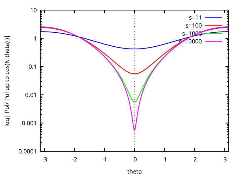
Figure 3: The graphs of $Pol(s,\cos(\theta))/Pol_{0}(s)$ and $Pol(s,\cos(\theta))/Pol_{4}(s)$ where $Pol_{N}(s)$ is $Pol(s,\cos(\theta))$ truncated to $\cos\left(N\theta\right)$ for different values of $s$ for the ordered partial amplitude $S4zTTT$.

In figure 4 we plot $Pol(s,\cos(\theta))/Pol_{0}(s)/(Den(s,\cos(\theta))/Den_{0}(s))$ where the logarithm of its absolute value in order to show that the amplitude is completely smooth

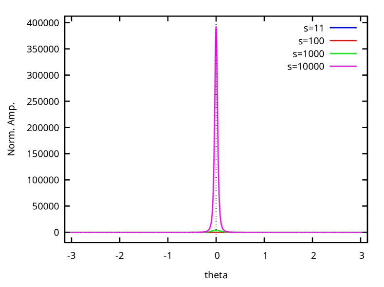
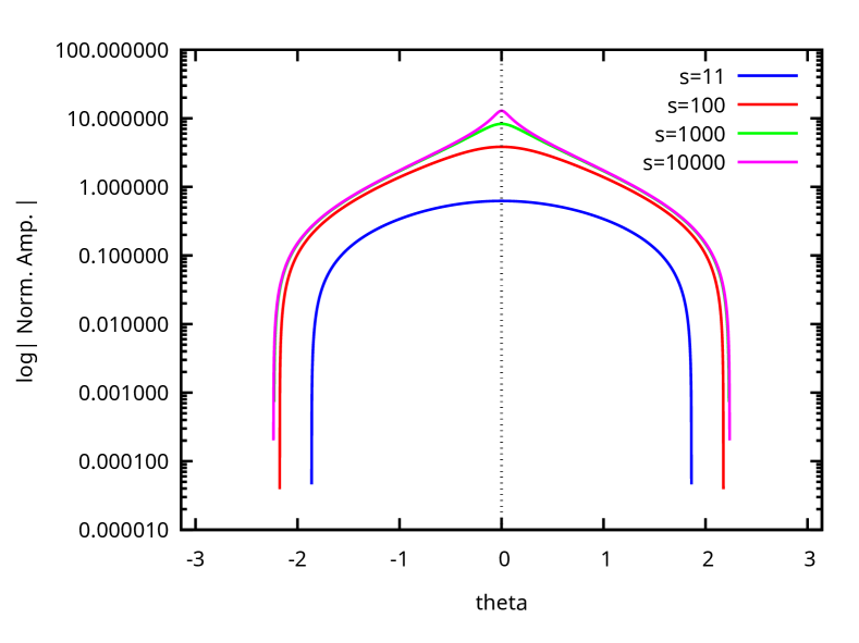
Figure 4: Two way of making the graphs for different $s$ values of the for the ordered partial amplitude $S4zTTT$ divided by Veneziano one. In the left figure the “normalized” amplitude and in the right one the logarithm of the absolute value.

4.1.2 $S10z1TTT$

This amplitude is $1$ massive scalar $|S10z1\rangle$ and $3$ tachyons $|T\rangle$.

For this amplitude the kinematics is given by

$$s+t+u=3,t=-{{\sqrt{s+2}\,\sqrt{{{s^{2}-8\,s+25}\over{s}}}\,\cos\theta-s-13}\over{2}}.$$ (4.7)

The amplitude can be written as a product of the Veneziano amplitude times a polynomial $Pol(s,t)$ in the Mandelstam variables $s$ and $t$ divided by another factorized rational function $Den(s,t)=R_{0}(s)R_{1}(t)$. Explicitly we get

$$A_{1234}= A_{\mbox{ Veneziano }1234}(s,t)\frac{Pol(s,t)}{Den(s,t)},$$ (4.8)

$$Pol( s,t)=(t+s-3)(19246080000\,s^{3}\,t^{8}+72307710400\,s^{2}\,t^{8}-495493590112\,s\,t^{8}$$

$$+209895950976\,t^{8}+76984320000\,s^{4}\,t^{7}+58277881600\,s^{3}\,t^{7}-2849666885248\,s^{2}\,t^{7}$$

$$+6785506885248\,s\,t^{7}-2518751411712\,t^{7}+134722560000\,s^{5}\,t^{6}-172135436800\,s^{4}\,t^{6}$$

$$-5425029925632\,s^{3}\,t^{6}+25387203880928\,s^{2}\,t^{6}-36484663001424\,s\,t^{6}+11902849553264\,t^{6}$$

$$+134722560000\,s^{6}\,t^{5}-316211216000\,s^{5}\,t^{5}-5953207313728\,s^{4}\,t^{5}+39558849014496\,s^{3}\,t^{5}$$

$$-96863042516112\,s^{2}\,t^{5}+97433269141344\,s\,t^{5}-27784976510448\,t^{5}+76984320000\,s^{7}\,t^{4}$$

$$-172135436800\,s^{6}\,t^{4}-5953207313728\,s^{5}\,t^{4}+41388340869920\,s^{4}\,t^{4}-120462310505520\,s^{3}\,t^{4}$$

$$+180747600195780\,s^{2}\,t^{4}-129476478679310\,s\,t^{4}+31073953964624\,t^{4}+19246080000\,s^{8}\,t^{3}$$

$$+58277881600\,s^{7}\,t^{3}-5425029925632\,s^{6}\,t^{3}+39558849014496\,s^{5}\,t^{3}-120462310505520\,s^{4}\,t^{3}$$

$$+187181862030920\,s^{3}\,t^{3}-152800662329140\,s^{2}\,t^{3}+58251056312116\,s\,t^{3}-7691084537808\,t^{3}$$

$$+72307710400\,s^{8}\,t^{2}-2849666885248\,s^{7}\,t^{2}+25387203880928\,s^{6}\,t^{2}-96863042516112\,s^{5}\,t^{2}$$

$$+180747600195780\,s^{4}\,t^{2}-152800662329140\,s^{3}\,t^{2}+19948948375074\,s^{2}\,t^{2}+43985153251806\,s\,t^{2}$$

$$-16275598612609\,t^{2}-495493590112\,s^{8}\,t+6785506885248\,s^{7}\,t-36484663001424\,s^{6}\,t$$

$$+97433269141344\,s^{5}\,t-129476478679310\,s^{4}\,t+58251056312116\,s^{3}\,t+43985153251806\,s^{2}\,t$$

$$-54451034393413\,s\,t+14367789889923\,t+209895950976\,s^{8}-2518751411712\,s^{7}$$

$$+11902849553264\,s^{6}-27784976510448\,s^{5}+31073953964624\,s^{4}-7691084537808\,s^{3}$$

$$-16275598612609\,s^{2}+14367789889923\,s-3375036340305,$$ (4.9)

$$Den(s,t)= {{\left(t-4\right)\,\left(t-3\right)\,\left(t-2\right)\,\left(t-1\right)\,\left(2\,t-7\right)\,\left(2\,t-5\right)\,\left(2\,t-3\right)\,\left(2\,t-1\right)\,\left(2\,t+1\right)}\over{8\,s}}.$$ (4.10)

Using as variables $s$ and $\cos\theta$ we get

$$Pol(s, \cos(\theta))=+{1\over{2048\,s^{4}}}\Big{\{}434225846880000\,s^{16}+13586375381224350\,s^{15}+158698806730129163\,s^{14}$$

$$+1020161896114142789\,s^{13}+4579911241197219728\,s^{12}+17983923513019837696\,s^{11}$$

$$+66094376516151198610\,s^{10}+166007805887694315654\,s^{9}-47280576652524084540\,s^{8}$$

$$-2338303115659298097246\,s^{7}-9644935380484900616757\,s^{6}-20319615386725921732643\,s^{5}$$

$$-21748603135802344243772\,s^{4}-6919512235240917629000\,s^{3}+4641203433233149430000\,s^{2}$$

$$+2246552769268171250000\,s+124830697406625000000\Big{\}}$$

$$-{\sqrt{s+2}\,\sqrt{s^{2}-8\,s+25}\over{2048\,s^{{{9}\over{2}}}}}\,\Big{\{}736835571360000\,s^{15}+24262494947904450\,s^{14}$$

$$+310148596362208203\,s^{13}+2199866322977519268\,s^{12}+10011453883903583528\,s^{11}$$

$$+29729357594001574096\,s^{10}+38746929206901384358\,s^{9}-150333771984491223044\,s^{8}$$

$$-1109356709541965494992\,s^{7}-3363986780240184241154\,s^{6}-5487084661506553542041\,s^{5}$$

$$-4009753948867886698464\,s^{4}+33125286565046683600\,s^{3}+1101522481833913910000\,s^{2}$$

$$+187160156942239250000\,s+2582704084275000000\Big{\}}\,\cos\theta$$

$$+{{\left(s+2\right)\,\left(s^{2}-8\,s+25\right)}\over{256\,s^{4}}}\,\Big{\{}56148634080000\,s^{13}+1801934447514450\,s^{12}$$

$$+22331557269845881\,s^{11}+147556160792762677\,s^{10}+551391530479268838\,s^{9}$$

$$+824975497024579231\,s^{8}-2586772503079804850\,s^{7}-18131199005406798729\,s^{6}$$

$$-48192515547154547318\,s^{5}-65244043685360789933\,s^{4}-30741438619601576931\,s^{3}$$

$$+12716439042329819400\,s^{2}+8290308977370322500\,s+499322789626500000\Big{\}}\,\cos\left(2\,\theta\right)$$

$$-{{\left(s+2\right)^{{{3}\over{2}}}\,\left(s^{2}-8\,s+25\right)^{{{3}\over{2}}}}\over{1024\,s^{{{9}\over{2}}}}}\,\Big{\{}97883758560000\,s^{12}+2882735520388750\,s^{11}$$

$$+32071580344395329\,s^{10}+177098275192619080\,s^{9}+430500134866172693\,s^{8}$$

$$-431850542916384770\,s^{7}-5841902527073598625\,s^{6}-15917743691482524196\,s^{5}$$

$$-18528851747527062225\,s^{4}-4125362869305550488\,s^{3}+5038031818605182500\,s^{2}$$

$$+1117036798856370000\,s+17218027228500000\Big{\}}\,\cos\left(3\,\theta\right)$$

$$+{{\left(s+2\right)^{2}\,\left(s^{2}-8\,s+25\right)^{2}}\over{512\,s^{4}}}\,\Big{\{}15144860640000\,s^{10}+391084046314150\,s^{9}$$

$$+3660893262690279\,s^{8}+14812942985624393\,s^{7}+8669516428982718\,s^{6}$$

$$-139702638966315980\,s^{5}-476935951377989117\,s^{4}-522015650788573663\,s^{3}$$

$$+25227054251024984\,s^{2}+127647177650575500\,s+9986455792530000\Big{\}}\,\cos\left(4\,\theta\right),$$

$$-{{\left(s+2\right)^{{{5}\over{2}}}\,\left(s^{2}-8\,s+25\right)^{{{5}\over{2}}}}\over{1024\,s^{{{9}\over{2}}}}}\,\Big{\{}6592383840000\,s^{9}+143270621868950\,s^{8}$$

$$+1040743900056353\,s^{7}+2309530706794960\,s^{6}-6706305662443536\,s^{5}$$

$$-39403580070878872\,s^{4}-48009668427475285\,s^{3}+13983512810678086\,s^{2}$$

$$+7360636133489000\,s+147583090530000\Big{\}}\,\cos\left(5\,\theta\right)$$

$$+{{\left(s+2\right)^{3}\,\left(s^{2}-8\,s+25\right)^{3}}\over{256\,s^{4}}}\,\Big{\{}247191840000\,s^{7}+4301403433950\,s^{6}$$

$$+21046680815879\,s^{5}-3613948951853\,s^{4}-255771188812900\,s^{3}$$

$$-427537104413983\,s^{2}+186420616717031\,s+28532730835800\Big{\}}\,\cos\left(6\,\theta\right)$$

$$-{{\left(s+2\right)^{{{7}\over{2}}}\,\left(s^{2}-8\,s+25\right)^{{{7}\over{2}}}}\over{4096\,s^{{{9}\over{2}}}}}\,\Big{\{}390334560000\,s^{6}+5040314686750\,s^{5}$$

$$+11199363318817\,s^{4}-55978899789516\,s^{3}-168304511698887\,s^{2}$$

$$+81059422245766\,s+2951661810600\Big{\}}\,\cos\left(7\,\theta\right)$$

$$+{{\left(s+2\right)^{4}\,\left(19\,s+87\right)\,\left(s^{2}-8\,s+25\right)^{4}}\over{2048\,s^{4}}}\,\Big{\{}601440000\,s^{3}+2259615950\,s^{2}-15484174691\,s+6559248468\Big{\}}\,\cos\left(8\,\theta\right)$$

$$-{{\left(s+2\right)^{{{9}\over{2}}}\,\left(s^{2}-8\,s+25\right)^{{{9}\over{2}}}}\over{4096\,s^{{{9}\over{2}}}}}\,\Big{\{}601440000\,s^{3}+2259615950\,s^{2}-15484174691\,s+6559248468\Big{\}}\,\cos\left(9\,\theta\right),$$ (4.11)

$$Den(s, \cos(\theta))=+{1\over{16384\,s^{5}}}\Big{\{}12155\,s^{13}+373230\,s^{12}+5108532\,s^{11}+42774600\,s^{10}+264628434\,s^{9}$$

$$+1422487220\,s^{8}+7205112140\,s^{7}+33813828856\,s^{6}+143312204283\,s^{5}$$

$$+576955276206\,s^{4}+1239531123000\,s^{3}+1108897510000\,s^{2}+321623750000\,s+17937500000\Big{\}}$$

$$-{{\sqrt{s+2}\,\sqrt{s^{2}-8\,s+25}}\over{16384\,s^{{{11}\over{2}}}}}\,\Big{\{}21879\,s^{12}+721864\,s^{11}+10834824\,s^{10}+100784376\,s^{9}$$

$$+679294630\,s^{8}+3695817944\,s^{7}+17182228584\,s^{6}+67849495976\,s^{5}$$

$$+211094027547\,s^{4}+321419947200\,s^{3}+181434995000\,s^{2}+26131000000\,s+393750000\Big{\}}\,\cos\left(\theta\right)$$

$$+{{\left(s+2\right)\,\left(s^{2}-8\,s+25\right)}\over{2048\,s^{5}}}\,\Big{\{}1989\,s^{10}+67340\,s^{9}+1037582\,s^{8}+9801330\,s^{7}+64807225\,s^{6}+322377384\,s^{5}$$

$$+1223081220\,s^{4}+3229212058\,s^{3}+3599119300\,s^{2}+1196895000\,s+71750000\Big{\}}\,\cos\left(2\,\theta\right)$$

$$-{{\left(s+2\right)^{{{3}\over{2}}}\,\left(s^{2}-8\,s+25\right)^{{{3}\over{2}}}}\over{8192\,s^{{{11}\over{2}}}}}\,\Big{\{}4641\,s^{9}+154518\,s^{8}+2306941\,s^{7}+20486858\,s^{6}+120087359\,s^{5}$$

$$+474259618\,s^{4}+1138931239\,s^{3}+898829750\,s^{2}+156502500\,s+2625000\Big{\}}\,\cos\left(3\,\theta\right)$$

$$+{{7\,\left(s+2\right)^{2}\,\left(s^{2}-8\,s+25\right)^{2}}\over{4096\,s^{5}}}\,\Big{\{}153\,s^{7}+4790\,s^{6}+65146\,s^{5}+497748\,s^{4}$$

$$+2249225\,s^{3}+5342014\,s^{2}+2725500\,s+205000\Big{\}}\,\cos\left(4\,\theta\right)$$

$$-{{\left(s+2\right)^{{{5}\over{2}}}\,\left(s^{2}-8\,s+25\right)^{{{5}\over{2}}}}\over{8192\,s^{{{11}\over{2}}}}}\,\Big{\{}765\,s^{6}+21340\,s^{5}+244016\,s^{4}+1402140\,s^{3}+3648027\,s^{2}+1042000\,s+22500\Big{\}}\,\cos\left(5\,\theta\right)$$

$$+{{\left(s+2\right)^{3}\,\left(s^{2}-8\,s+25\right)^{3}}\over{2048\,s^{5}}}\,\Big{\{}51\,s^{4}+1176\,s^{3}+9928\,s^{2}+31862\,s+4100\Big{\}}\,\cos\left(6\,\theta\right)$$

$$-{{\left(s+2\right)^{{{7}\over{2}}}\,\left(s^{2}-8\,s+25\right)^{{{7}\over{2}}}\,\Big{\{}153\,s^{3}+2570\,s^{2}+11897\,s+450\Big{\}}\,}\over{32768\,s^{{{11}\over{2}}}}}\cos\left(7\,\theta\right)$$

$$+{{\left(s+2\right)^{4}\,\left(9\,s+82\right)\,\left(s^{2}-8\,s+25\right)^{4}\,}\over{16384\,s^{5}}}\cos\left(8\,\theta\right)$$

$$-{{\left(s+2\right)^{{{9}\over{2}}}\,\left(s^{2}-8\,s+25\right)^{{{9}\over{2}}}\,}\over{32768\,s^{{{11}\over{2}}}}}\cos\left(9\,\theta\right).$$ (4.12)

Using the previous result we can plot in figure 5 $Pol(s,\cos(\theta))/Pol_{0}(s)$ and $Pol(s,\cos(\theta))/Pol_{4}(s)$ where $Pol_{N}(s)$ is $Pol(s,\cos(\theta))$ truncated to $\cos\left(N\theta\right)$ in order to show that $Pol_{0}(s)$ is essentially the main contribution.

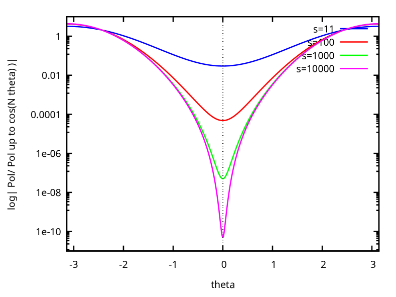
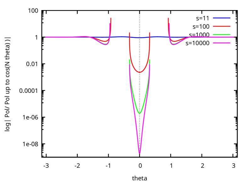
Figure 5: The graphs of $Pol(s,\cos(\theta))/Pol_{0}(s)$ and $Pol(s,\cos(\theta))/Pol_{4}(s)$ where $Pol_{N}(s)$ is $Pol(s,\cos(\theta))$ truncated to $\cos\left(n\theta\right)$ for different values of $s$ for the amplitude $S10z1TTT$.

In figure 6 we plot $Pol(s,\cos(\theta))/Pol_{0}(s)/(Den(s,\cos(\theta))/Den_{0}(s))$ where the logarithm of its absolute value in order to show that the amplitude is completely smooth

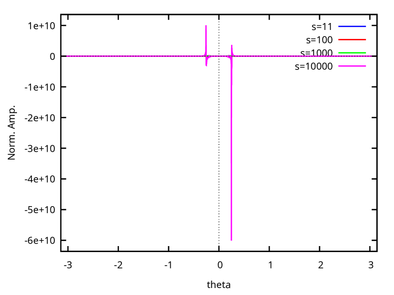
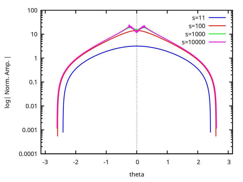
Figure 6: Two way of making the graphs for different $s$ values of the for the ordered partial amplitude $S10z1TTT$. divided by Veneziano one. In the left figure the “normalized” amplitude and in the right one the logarithm of the absolute value.

4.1.3 $S10z2TTT$

This amplitude is $1$ massive scalar $|S10z2\rangle$ and $3$ tachyons $|T\rangle$.

In this case we report only the analogous graphs we discussed in the previous sections. They are in figures 7 and 8 qualitatively similar.

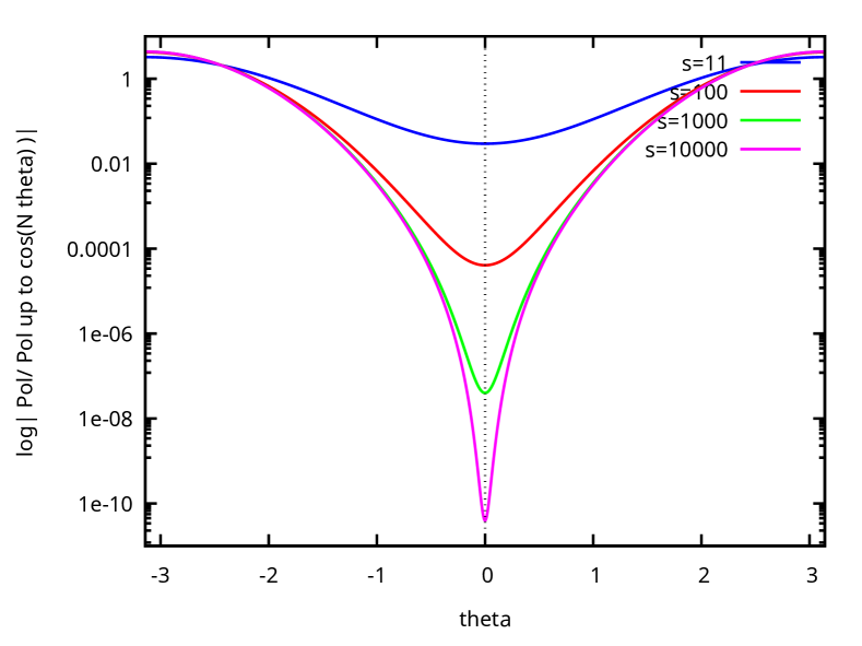
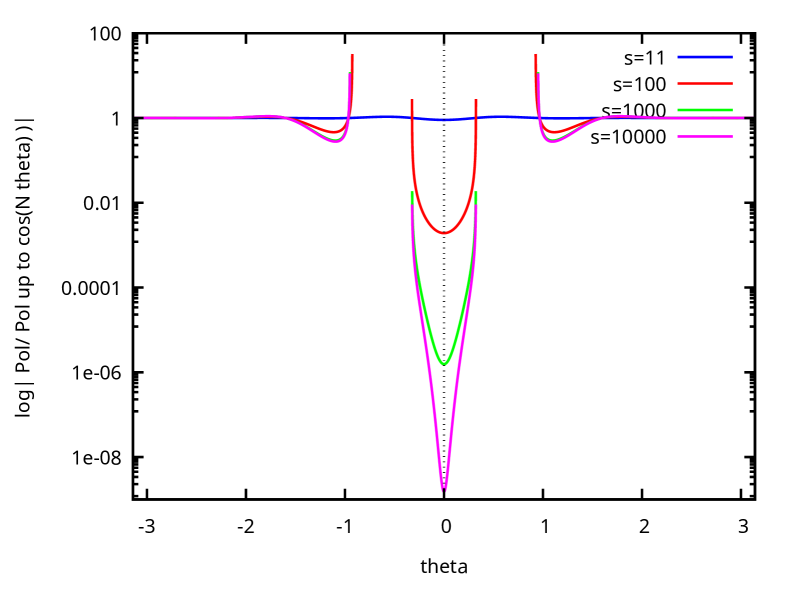
Figure 7: The graphs of $Pol(s,\cos(\theta))/Pol_{0}(s)$ and $Pol(s,\cos(\theta))/Pol_{4}(s)$ where $Pol_{N}(s)$ is $Pol(s,\cos(\theta))$ truncated to $\cos\left(N\theta\right)$ for different values of $s$ for the amplitude $S10z2TTT$.

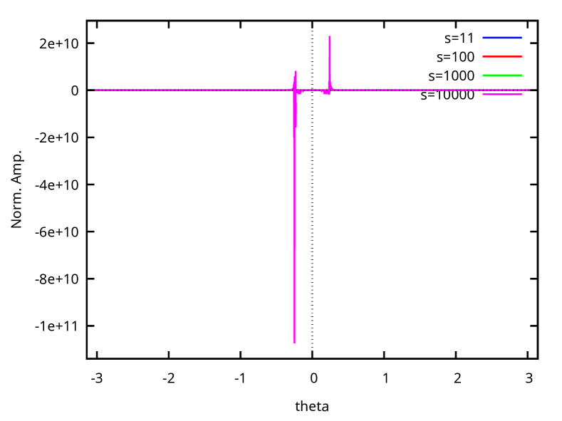
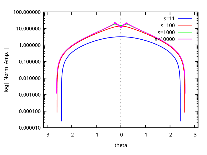
Figure 8: Two way of making the graphs for different $s$ values of the for the ordered partial amplitude $S10z2TTT$. divided by Veneziano one. In the left figure the “normalized” amplitude and in the right one the logarithm of the absolute value.

4.2 Amplitudes with two massive scalar and two tachyons

We can now exam the case of two massive non tachyonic scalars and two tachyons. The results are again qualitatively similar to the simpler cases of the previous section.

In this case we report $S10z1S10z1TT$ only since it is the amplitude with the highest $t$ power, i.e. $t^{19}\sim\cos(19\theta)$.

4.2.1 $S10z1S10z1TT$

This amplitude is $2$ massive scalars $|S10z1\rangle$, and $2$ tachyons $|T\rangle$.

The leading order of $Pol(s,t)$ reads

$$Pol(s,t)= (t+s-8)\Big{\{}185205797683200000000\,s^{8}\,t^{18}+24542364689375232000000\,s^{7}\,t^{18}$$

$$-2874513043747520346880000\,s^{6}\,t^{18}+602740879101585150468915200\,s^{5}\,t^{18}+\dots\Big{\}}.$$ (4.13)

In this case we report only the analogous graphs we discussed in the previous sections. They are qualitatively similar.

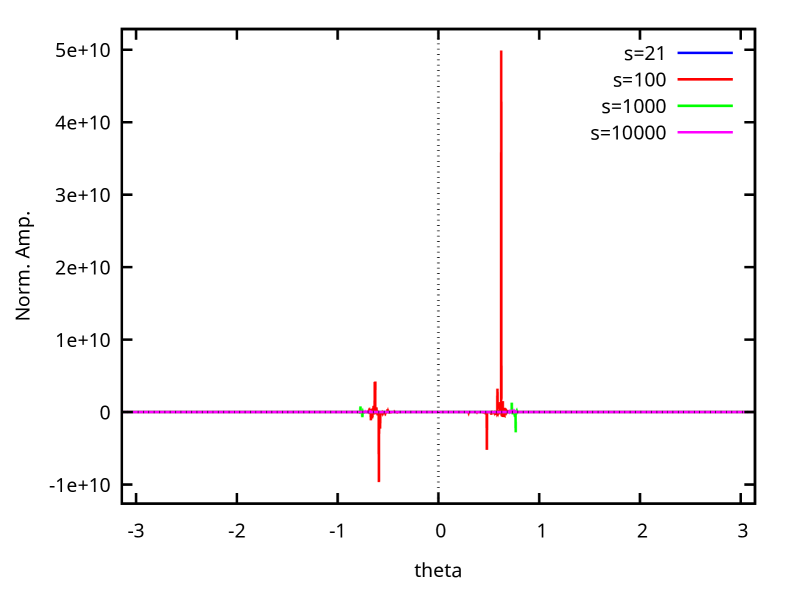
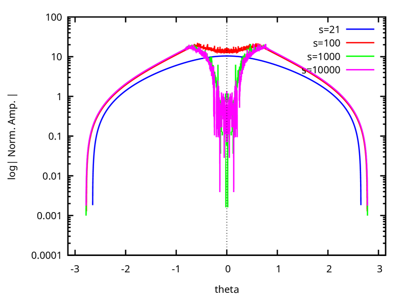
Figure 10: Two way of making the graphs for different $s$ values of the for the ordered partial amplitude $S10z1S10z1TT$. divided by Veneziano one. In the left figure the “normalized” amplitude and in the right one the logarithm of the absolute value.

4.3 Amplitudes with three massive scalar and one tachyon

We can now exam the three non tachyonic massive scalars and one tachyon cases. We report the most “complex” case we have computed.

4.3.1 $S6zS6zS4zT$

This amplitude is $2$ massive scalars $|S6z\rangle$, $1$ massive scalar $|S4z\rangle$ and $1$ tachyons $|T\rangle$.

The leading order of $Pol(s,t)$ reads

$$Pol(s,t)= (t+s-6)(2\,t+2\,s-11)\Big{\{}12800\,s^{7}\,t^{12}$$

$$+132480\,s^{6}\,t^{12}+958592\,s^{5}\,t^{12}+3844320\,s^{4}\,t^{12}+\dots\Big{\}}.$$ (4.14)

In this case we report again only the analogous graphs we discussed in the previous sections. This is done in figures 11 and 12.

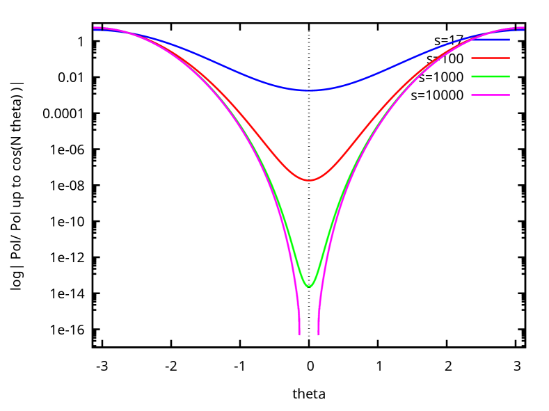
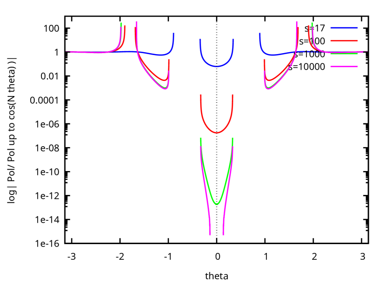
Figure 11: The graphs of $Pol(s,\cos(\theta))/Pol_{0}(s)$ and $Pol(s,\cos(\theta))/Pol_{4}(s)$ where $Pol_{N}(s)$ is $Pol(s,\cos(\theta))$ truncated to $\cos\left(N\theta\right)$ for different values of $s$ for the amplitude $S6zS6zS4zT$.

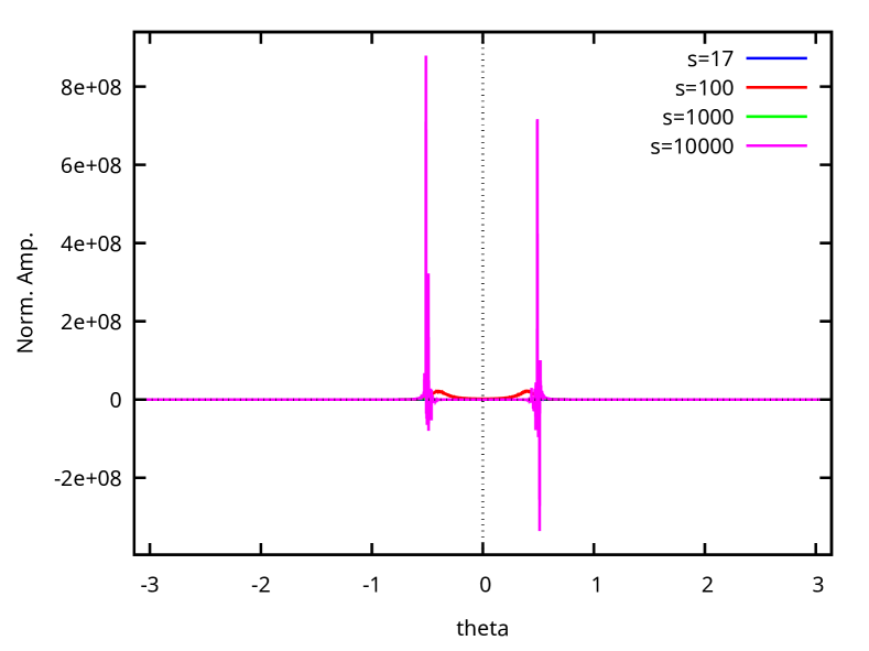
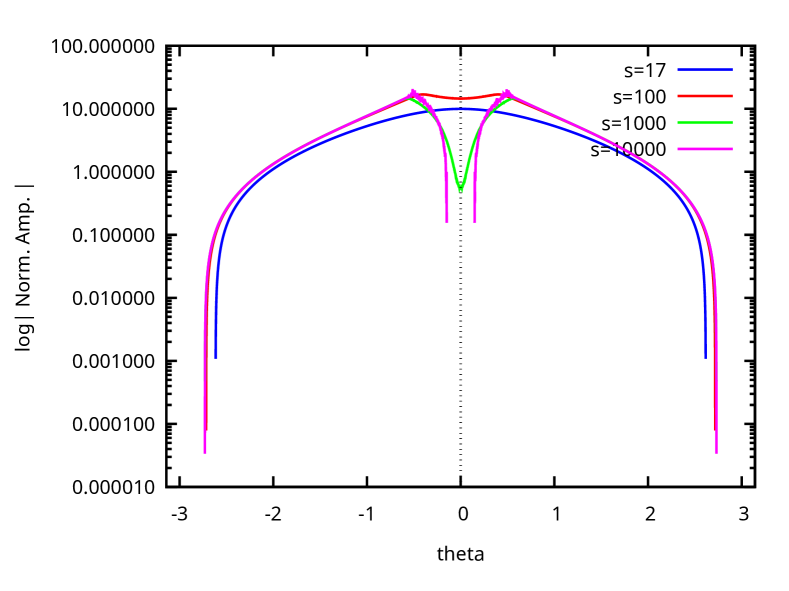
Figure 12: Two way of making the graphs for different $s$ values of the for the ordered partial amplitude $S6zS6zS4zT$. divided by Veneziano one. In the left figure the “normalized” amplitude and in the right one the logarithm of the absolute value.

References

- [1] David Mitchell and Bo Sundborg “Measuring the size and shape of strings” In Nucl. Phys. B 349, 1991, pp. 159–167 DOI: 10.1016/0550-3213(91)90192-Z
- [2] Juan L. Manes “Emission spectrum of fundamental strings: An Algebraic approach” In Nucl. Phys. B 621, 2002, pp. 37–61 DOI: 10.1016/S0550-3213(01)00578-8
- [3] Juan L. Manes “String form-factors” In JHEP 01, 2004, pp. 033 DOI: 10.1088/1126-6708/2004/01/033
- [4] Juan L. Manes “Portrait of the string as a random walk” In JHEP 03, 2005, pp. 070 DOI: 10.1088/1126-6708/2005/03/070
- [5] Roberto Iengo and Jorge G. Russo “The Decay of massive closed superstrings with maximum angular momentum” In JHEP 11, 2002, pp. 045 DOI: 10.1088/1126-6708/2002/11/045
- [6] Roberto Iengo and Jorge G. Russo “Semiclassical decay of strings with maximum angular momentum” In JHEP 03, 2003, pp. 030 DOI: 10.1088/1126-6708/2003/03/030
- [7] Diego Chialva, Roberto Iengo and Jorge G. Russo “Decay of long-lived massive closed superstring states: Exact results” In JHEP 12, 2003, pp. 014 DOI: 10.1088/1126-6708/2003/12/014
- [8] Diego Chialva and Roberto Iengo “Long lived large type II strings: Decay within compactification” In JHEP 07, 2004, pp. 054 DOI: 10.1088/1126-6708/2004/07/054
- [9] Diego Chialva, Roberto Iengo and Jorge G. Russo “Search for the most stable massive state in superstring theory” In JHEP 01, 2005, pp. 001 DOI: 10.1088/1126-6708/2005/01/001
- [10] Roberto Iengo and Jorge G. Russo “Handbook on string decay” In JHEP 02, 2006, pp. 041 DOI: 10.1088/1126-6708/2006/02/041
- [11] Roberto Iengo “Massless radiation from strings: Quantum spectrum average statistics and cusp-kink configurations” In JHEP 05, 2006, pp. 054 DOI: 10.1088/1126-6708/2006/05/054
- [12] R. Iengo and J. Russo “Black hole formation from collisions of cosmic fundamental strings” In JHEP 08, 2006, pp. 079 DOI: 10.1088/1126-6708/2006/08/079
- [13] Andrea Arduino, Riccardo Finotello and Igor Pesando “On the origin of divergences in time-dependent orbifolds” In Eur. Phys. J. C 80.5, 2020, pp. 476 DOI: 10.1140/epjc/s10052-020-8010-y
- [14] Zvi Bern et al. “Spinning black hole binary dynamics, scattering amplitudes, and effective field theory” In Phys. Rev. D 104.6, 2021, pp. 065014 DOI: 10.1103/PhysRevD.104.065014
- [15] Lucile Cangemi and Paolo Pichini “Classical limit of higher-spin string amplitudes” In JHEP 06, 2023, pp. 167 DOI: 10.1007/JHEP06(2023)167
- [16] Lucile Cangemi et al. “Kerr Black Holes From Massive Higher-Spin Gauge Symmetry” In Phys. Rev. Lett. 131.22, 2023, pp. 221401 DOI: 10.1103/PhysRevLett.131.221401
- [17] Joseph Polchinski “String theory and black hole complementarity” In STRINGS 95: Future Perspectives in String Theory, 1995, pp. 417–426 arXiv:hep-th/9507094
- [18] Gary T. Horowitz and Joseph Polchinski “A Correspondence principle for black holes and strings” In Phys. Rev. D 55, 1997, pp. 6189–6197 DOI: 10.1103/PhysRevD.55.6189
- [19] Gary T. Horowitz and Joseph Polchinski “Selfgravitating fundamental strings” In Phys. Rev. D 57, 1998, pp. 2557–2563 DOI: 10.1103/PhysRevD.57.2557
- [20] Thibault Damour and Gabriele Veneziano “Selfgravitating fundamental strings and black holes” In Nucl. Phys. B 568, 2000, pp. 93–119 DOI: 10.1016/S0550-3213(99)00596-9
- [21] G. Veneziano “Quantum hair and the string-black hole correspondence” In Class. Quant. Grav. 30, 2013, pp. 092001 DOI: 10.1088/0264-9381/30/9/092001
- [22] J.. Manes and Maria A.. Vozmediano “A Simple Construction of String Vertex Operators” In Nucl. Phys. B 326, 1989, pp. 271–284 DOI: 10.1016/0550-3213(89)90444-6
- [23] Massimo Bianchi, Luca Lopez and Robert Richter “On stable higher spin states in Heterotic String Theories” In JHEP 03, 2011, pp. 051 DOI: 10.1007/JHEP03(2011)051
- [24] Chrysoula Markou and Evgeny Skvortsov “An excursion into the string spectrum” In JHEP 12, 2023, pp. 055 DOI: 10.1007/JHEP12(2023)055
- [25] E. Del Giudice, P. Di Vecchia and S. Fubini “General properties of the dual resonance model” In Annals Phys. 70, 1972, pp. 378–398 DOI: 10.1016/0003-4916(72)90272-2
- [26] M. Ademollo, E. Del Giudice, P. Di Vecchia and S. Fubini “Couplings of three excited particles in the dual-resonance model” In Nuovo Cim. A 19, 1974, pp. 181–203 DOI: 10.1007/BF02801846
- [27] Klaus Hornfeck “Three Reggeon Light Cone Vertex of the Neveu-schwarz String” In Nucl. Phys. B 293, 1987, pp. 189 DOI: 10.1016/0550-3213(87)90068-X
- [28] Mark Hindmarsh and Dimitri Skliros “Covariant Closed String Coherent States” In Phys. Rev. Lett. 106, 2011, pp. 081602 DOI: 10.1103/PhysRevLett.106.081602
- [29] Dimitri Skliros and Mark Hindmarsh “String Vertex Operators and Cosmic Strings” In Phys. Rev. D 84, 2011, pp. 126001 DOI: 10.1103/PhysRevD.84.126001
- [30] Massimo Bianchi and Maurizio Firrotta “DDF operators, open string coherent states and their scattering amplitudes” In Nucl. Phys. B 952, 2020, pp. 114943 DOI: 10.1016/j.nuclphysb.2020.114943
- [31] David J. Gross and Vladimir Rosenhaus “Chaotic scattering of highly excited strings” In JHEP 05, 2021, pp. 048 DOI: 10.1007/JHEP05(2021)048
- [32] Vladimir Rosenhaus “Chaos in a Many-String Scattering Amplitude” In Phys. Rev. Lett. 129.3, 2022, pp. 031601 DOI: 10.1103/PhysRevLett.129.031601
- [33] Maurizio Firrotta and Vladimir Rosenhaus “Photon emission from an excited string” In JHEP 09, 2022, pp. 211 DOI: 10.1007/JHEP09(2022)211
- [34] Koji Hashimoto, Yoshinori Matsuo and Takuya Yoda “Transient chaos analysis of string scattering” In JHEP 11, 2022, pp. 147 DOI: 10.1007/JHEP11(2022)147
- [35] Maurizio Firrotta “The chaotic emergence of thermalization in highly excited string decays” In JHEP 04, 2023, pp. 052 DOI: 10.1007/JHEP04(2023)052
- [36] Nikola Savić and Mihailo Čubrović “Weak chaos and mixed dynamics in the string S-matrix” In JHEP 03, 2024, pp. 101 DOI: 10.1007/JHEP03(2024)101
- [37] Dripto Biswas and Igor Pesando “Framed DDF operators and the general solution to Virasoro constraints” In Eur. Phys. J. C 84.7, 2024, pp. 657 DOI: 10.1140/epjc/s10052-024-12883-7
- [38] Maurizio Firrotta “Veneziano and Shapiro-Virasoro amplitudes of arbitrarily excited strings”, 2024 arXiv:2402.16183 [hep-th]
- [39] Maurizio Firrotta, Elias Kiritsis and Vasilis Niarchos “Scattering, Absorption and Emission of Highly Excited Strings”, 2024 arXiv:2407.16476 [hep-th]
- [40] Aranya Bhattacharya and Aneek Jana “Quantum chaos and complexity from string scattering amplitudes”, 2024 arXiv:2408.11096 [hep-th]
- [41] Dripto Biswas, Raffaele Marotta and Igor Pesando “The Reggeon Vertex for DDF States”, 2024 arXiv:2410.17093 [hep-th]
- [42] Theodore Erler and Hiroaki Matsunaga “Mapping between Witten and lightcone string field theories” In JHEP 11, 2021, pp. 208 DOI: 10.1007/JHEP11(2021)208
- [43] Theodore Erler “Open string field theory in lightcone gauge”, 2024 arXiv:2412.05069 [hep-th]
- [44] Dripto Biswas and Igor Pesando “DDF amplitudes are lightcone amplitudes and the naturalness of Mandelstam map”, 2024 arXiv:2411.06109 [hep-th]
- [45] Vladimir Rosenhaus “Chaos in the Quantum Field Theory S-Matrix” In Phys. Rev. Lett. 127.2, 2021, pp. 021601 DOI: 10.1103/PhysRevLett.127.021601
- [46] Diptarka Das, Santanu Mandal and Anurag Sarkar “Chaotic and thermal aspects in the highly excited string S-matrix” In JHEP 08, 2024, pp. 200 DOI: 10.1007/JHEP08(2024)200
- [47] Massimo Bianchi, Maurizio Firrotta, Jacob Sonnenschein and Dorin Weissman “Measure for Chaotic Scattering Amplitudes” In Phys. Rev. Lett. 129.26, 2022, pp. 261601 DOI: 10.1103/PhysRevLett.129.261601
- [48] Massimo Bianchi, Maurizio Firrotta, Jacob Sonnenschein and Dorin Weissman “Measuring chaos in string scattering processes” In Phys. Rev. D 108.6, 2023, pp. 066006 DOI: 10.1103/PhysRevD.108.066006
- [49] Massimo Bianchi, Maurizio Firrotta, Jacob Sonnenschein and Dorin Weissman “From spectral to scattering form factor” In JHEP 06, 2024, pp. 189 DOI: 10.1007/JHEP06(2024)189
- [50] Thomas Basile and Chrysoula Markou “On the deep superstring spectrum” In JHEP 07, 2024, pp. 184 DOI: 10.1007/JHEP07(2024)184
- [51] Igor Pesando “The bosonic string spectrum and the explicit states up to level from the lightcone and the chaotic behavior of certain string amplitudes”, 2024 arXiv:2405.09987 [hep-th]
- [52] Thomas L. Curtright and Charles B. Thorn “Symmetry Patterns in the Mass Spectra of Dual String Models” In Nucl. Phys. B 274, 1986, pp. 520–558 DOI: 10.1016/0550-3213(86)90525-0
- [53] Thomas Curtright “COUNTING SYMMETRY PATTERNS IN THE SPECTRA OF STRINGS” In Informal Summer Institute on Superstrings, 1986
- [54] T.. Curtright, G.. Ghandour and Charles B. Thorn “Spin Content of String Models” In Phys. Lett. B 182, 1986, pp. 45–52 DOI: 10.1016/0370-2693(86)91076-2