Time scale competition in the Active Coagulation Model
Abstract
Spreading processes on top of active dynamics provide a novel theoretical framework for capturing emerging collective behavior in living systems. I consider run-and-tumble dynamics coupled with coagulation/decoagulation reactions that lead to an absorbing state phase transition. While the active dynamics does not change the location of the transition point, the relaxation toward the stationary state depends on motility parameters. Because of the competition between spreading dynamics and active motion, the system can support long-living currents whose typical time scale is a nontrivial function of motility and reaction rates. Beyond the mean-field regime, instability at finite length scales regulates a crossover from periodic to diffusive modes. Finally, it is possible to individuate different mechanisms of pattern formation on a large time scale, ranging from Fisher-Kolmogorov to Kardar-Parisi-Zhang equation.
I Introduction
While Newton’s third law imposes a strong constraint, symmetrical interactions are the exception rather than the rule in the biological world. Examples include social interactions [1], the synaptic dynamics in neural nets [2], to biochemical reactions [3]. Breaking symmetric interaction rules is another way to fall out of equilibrium [4]. Recent studies have focused on non-symmetric interactions, particularly at the mesoscopic level [5, 6], in both numerical simulations and coarse-graining theory [7], as well as minimal mixed spin models with distinct interaction rules for different spin variables [8]. This work focuses on the simplest scenario, familiar in statistical physics: reaction rules that are inherently non-symmetrical and typically lead to absorbing states, which break detailed balance [3]. This scenario naturally connects to the broader question of how spreading processes (e.g., SIS or SIR dynamics [9]) are affected by active dynamics. More generally, it explores the collective behavior arising from coupled self-propelled motion and contagious dynamics [10, 11, 12, 13, 14, 15, 16, 17, 18, 19, 20, 21, 22].
Here, I consider a minimal coagulation process coupled with run-and-tumble dynamics. A simple example of this reaction dynamics is population growth. The coagulation model describes a single species undergoing coagulation and decoagulation reactions (e.g., birth and death processes), which change the number of particles. These reactions introduce additional time scales that compete with those of the active dynamics.
Once we add self-propulsion, we can think of the model as a model of self-propelled agents that annihilate at a rate and spontaneously duplicate at a rate . While other active matter models with birth processes have been explored [23, 24], this work focuses on how the competition of time scales generates interesting phenomena, even in a simple gas of active particles. This work shows that assuming rapidly decaying currents as a closure for the density field’s time evolution is problematic when multiple time scales are present. I show that long-living currents arise from the density-current coupling, where the coagulation rate is the coupling constant. When this coupling is not negligible, the system requires increasingly longer times to reach a stationary state. This increased relaxation time is associated with damped traveling waves that do not always relax monotonically to the stationary state.
II Active Coagulation Model
Adopting the standard notation for run-and-tumble active particles in one spatial dimension, and indicate the fraction of right-moving and left-moving particles, respectively [25]. The active motion is characterized by the self-propulsion velocity and the tumbling rate . In the limit and with fixed diffusion constant , the random walk reduces to the standard Brownian motion. On top of the active motion, I consider a coagulation process characterized by two parameters. In the following, indicates the reaction rate of the coagulation reaction, and with the rate of the offspring production (decoagulation). In other words, if indicates the presence of an active particle in some point of space at a given time, and indicates no particles, within coagulation dynamics one has to consider two elementary processes: the coagulation process that tends to annihilate particles, i.e, a particle spontaneously disappears, and the decoagulation process which introduces a new particle. After adding self-propelled motion, the set of reactions are
| (1) | |||
I will employ these three elementary processes in the following fashion
| (2) | ||||
| (3) |
once one introduces the current and the probability density , the equations of motion for and are
| (4) | ||||
| (5) | ||||
| (6) |
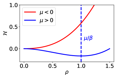
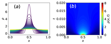
is a functional of the density field . The quadratic term generates linear interactions that tend to bring the system to extinction. Non-linear interactions are therefore essential for the existence of stationary solutions with . The nonlinearities in (4) generally render the dynamics analytically intractable. Fig. (1) depicts the typical behavior of as the mass term changes from negative to positive values. Since represents a rate, negative values are physically meaningless. The parameter should be understood as relative to a reference value In this work, I choose so negative values of correspond to . In the first case, the equilibrium configuration is the absorbing state . In the second, it is the mixed state . The current-density interaction in (5) introduces an additional level of complexity compared to standard reaction-diffusion models.
It is worth recalling the picture without coagulation dynamics where the equations for and become
| (7) | ||||
| (8) |
In this case, the dynamics of the system is governed by a second-order differential equation that can be obtained simply by computing so that
| (9) |
This telegrapher equation predicts wave propagation on short-time scales that eventually diffuse [26]. One can rationalize that studying the limiting case at fixed diffusive constant that reproduce the standard diffusive equation
| (10) |
while in the opposite limit one gets the standard wave equation
| (11) |
so that the model interpolates between a ballistic motion on time scales and a diffusive regime for . The presence of an additional dynamical process, as in the case of the coagulation dynamics considered here, introduces another time scale that enters in competition with . We also notice that, if we look at solutions of (7) and (8) that do not depend on space, i.e., mean-field like solutions and , one has and , i.e., and decouple from each other, the current decays on the time scale ( and the density is uniform
Well-Mixed Approximation
To understand what is the effect of an additional time scale, I first study the mean-field picture that one obtains by neglecting any spatial dependency of and so that . In this limit, one can find the analytical solution of the dynamics that turns out to be different from the standard RT dynamics where is constant and does not depend on (see (7)). The equation for is the well-known logistic equation
| (12) |
with the analytical solution (with the initial condition )
| (13) |
However, in contrast with a coagulation model in the mean-field approximation, in this case, there is still the equation for the current that has to be taken into account. For the current one gets (with )
| (14) |
whose solution reads
| (15) |
once one plugs (13) into (15) with initial condition it follows
| (16) | ||||
| (17) |
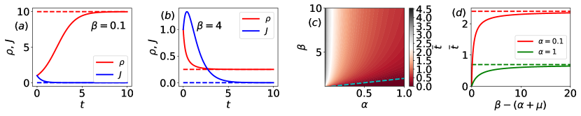
Figs. (2a,2b) report the typical behavior of and . Because of the persistent motion, one obtains non-trivial dynamics of the current that develops a peak before decaying to zero (see Fig. (2b)). In particular, the exponential decay rate of the current, that is in the case of RT dynamics, increases to thanks to birth processes that produce at the same rate left-handed and right-handed particles. However, the coagulation process controlled by tends to produce long-living currents (because of the coupling ) that generate the peak shown in Fig. (2b). One can compute the time when reaches its maximum value
| (18) |
with if (this condition is obtained using the fact that in (18)). Fig. (2c) reports the contour plot obtained through (18) with the color indicating the magnitude of . From the equation for , one obtains that in the diffusive limit , , while for finite tumbling rate one has . This asymptotic limit is shown in Fig. (2d).
This happens although the stationary states are the same as the coagulation model in the well-mixed approximation:
| (19) | ||||
| (20) |
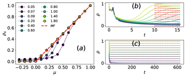
as one can also check by setting without solving the dynamics. On the other hand, while depends on , at the mean-field level, remains independent of . However, the mean-field computation suggests that non-trivial dynamics might be observed looking, for instance, at . To test the predictions of the mean-field theory, Fig. (3a) reports the numerical solution of the equations for and (here and ). The phase diagram has been obtained by varying for different values of the tumbling rate (here and ). One observes apparent deviations from the mean-field prediction at small as decreases (and thus the active motion becomes more important). Looking at the dynamics of , one obtains that at small (panel (b) in Fig. (3)) approaches its stationary mean-field value very slowly. On the contrary, as increases quickly converges to . One can connect this behavior with the fact that there is a characteristic time which maximizes the current . In other words, long-living currents slow down the relaxation time of producing an apparent violation of the mean-field prediction.
Linear Stability Analysis
From the previous section, it follows that the characteristic time scale on which decays depends on because it is coupled to through the coupling constant . This coupling, at the mean-field level, produces excess in that decays on a longer time scale (larger than ). Numerical solutions of the actual dynamics suggest that this effect impact also the dynamics of (that is transparent to in the mean-field picture). I now explore the spatiotemporal evolution of the spreading process combined with active motion in finite dimensions through the linear stability analysis of the stationary well-mixed configurations against small perturbations. As a standard procedure, one starts with
| (21) | ||||
| (22) |
the linearized dynamics for the perturbations reads
| (23) | ||||
| (24) |
Once one introduces , it is possible to rewrite in the compact form
| (25) | ||||
| (26) |
Looking at damped plane wave solutions , the dispersion relation controls the stability of the perturbation. is the solution of the eigenvalues equation
| (27) |
with eigenvalues
| (28) |
The stability condition requires and thus, for , one obtains and , so that the long-wavelength perturbation is always damped ensuring that density fluctuations are diffuse. However, for finite values, can acquire an imaginary part so that density fluctuations are dumped oscillations that propagate as waves. This happens whenever
| (29) |
and thus there is a critical wavelength given by
| (30) |
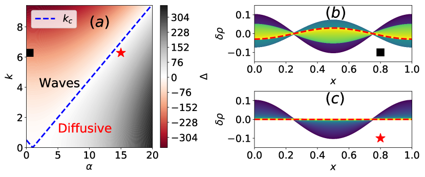
that separates purely diffusive excitations for from dumped travelling waves for . From (30) it follows that there is a limit where propagating waves dominate up to the macroscopic scale. This happen for so that . On the other hand, in the large tumbling rate limit there are only diffusive excitations. The linear stability analysis produces the phase diagram shown in Fig. (2a) that has been obtained for . To test this prediction one can solve numerically (4) and (5) (the initial condition is a small perturbation of the uniform profile with and periodic boundary conditions), with the initial condition on the current (with , ). In the case , one has so that linear stability predicts traveling waves. As one can see in Fig. (2b), that shows , the initial plane wave persists in the system while, in the second case (Fig. (2c)), , the initial wave dissipate fast into a uniform configuration without oscillations.
Dynamics towards the stationary state
Although one cannot analytically solve the non-linear dynamics in finite dimensions, it is possible to gain some insight into limiting cases. First, I consider the large limit. In this case, there are two possibilities: if the ratio is maintained finite, i.e., the Brownian limit of the run-and-tumble walker, the model reduces to reaction-diffusion in one spatial dimension. This limiting case can be understood by setting (5) in the following form
| (31) |
once the limit is performed, one arrives at the following constitutive relation for the current
| (32) |
once this expression of is inserted into the equation for , one arrives at the Fisher-Kolmogorov equation (see for instance [9])
| (33) |
Performing the same limit but at finite velocity , the diffusivity drops to zero, i.e., , and thus one ends with the well-mixed case because so that the dynamics reduces to (13). In this situation, the spreading process drives the system to uniform configurations so fast that active motion is irrelevant. This is also the case of with finite. There is another limit that is not trivial that I mention but I will not discuss. The case is and . In this limit, one can introduce a diffusion constant of the spreading process defined as . Since , the constitutive relation is that inserted into (4) brings to the following non-linear diffusion equation
| (34) |
In the opposite limit, one has as a small parameter so that the dynamics of and is the same as obtained within the linear stability analysis. At variance with the linear stability analysis, here as an initial condition, it is interesting to consider an arbitrary initial density profile that will move toward the stationary state characterized by and . Depending on the value of , the stationary state will be approached through traveling waves or purely dissipative modes. To test the different scenarios, equations (4) and (5) have been solved numerically with a Gaussian profile for as the initial condition (while is set to zero).
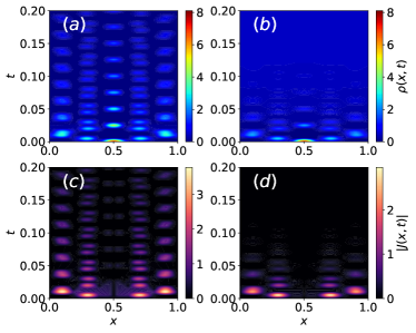
Fig. (5) reports the typical time evolution of the density field and the current field for two values of tumbling rate (). The reaction parameters are set and so that the stationary state is mixed (). In the case , the initial Gaussian profile propagates ballistically with a minimal attenuation, this is also mirrored by the behavior of that does not decay. On the contrary, as increases the traveling wave and currents tend to disappear rapidly. These long-living currents can be interpreted as Fisher waves preventing the system from quickly reaching a stationary uniform state.
Diffusive limit and pattern formation
In the case of time scales larger than the typical time scale of relaxation of , one can write a closed equation for . This is because once one imposes , it returns a constitutive relation . I refer to this situation as the diffusive limit. In this limit, the link between and is
| (35) | ||||
| (36) |
that brings us to the following diffusive equation
| (37) |
The dynamics of in this limit is poorly defined since becomes negative for large values. A negative diffusion constant might indicate pattern formation (for instance we can regularize the equation by inserting a surface term proportional to ). However, we have a divergent at that the surface tension term can not cure. This is because, in the assumption of fast decaying currents, one neglects situations where the coupling between active dynamics and the reaction process slows down the dynamics of , as observed in the previous sections. If is small enough, the diffusive limit is well-defined and thus the diffusion constant is not diverging and remains positive with . The dynamics is governed by an effective Fisher-Kolmogorov equation whose typical time-evolution is shown in Fig. (6).
Going back to (37), in the case of a perturbation around the uniform stationary state (we consider ), the dynamics of is controlled by
| (38) |
Again, this equation does not generally make sense unless one considers a small regime so that remains positive and finite. In the small limit, at the zero order in , can be replaced by , with renormalized by the spreading process, i.e., , so that one ends with a diffusive equation for the perturbation
| (39) |
A more interesting situation can be obtained if one keeps the first order in in the expression of . In particular, considering small perturbation so that , upon defining
| (40) | ||||
| (41) |
for , one has and thus
| (42) |
Adding a noise term to this equation (representing the effect of the fast degrees of freedom), brings us to
| (43) |
with , , and (with setting the strength of the noise). Considering fluctuations due to the noise around the absorbing state critical point , it follows that (43) is formally equivalent to Kardar-Parisi-Zhang equation (KPZ) model [27] (but with a non-linear diffusion coefficient). This mapping suggests that pattern formation at criticality should fall into the KPZ universality class. It is interesting to note that the strength of the KPZ term depends on the ratio , and thus on both autonomous motion and replication.
III Conclusions and Outlook
This work addresses a simple one-dimensional continuum model that combines two non-equilibrium phenomena: active dynamics and absorbing state phase transitions. The continuum model consists of a gas of run-and-tumble particles (for simplicity, one spatial dimension, generalization in dimensions is straightforward) that interacts via a reaction process that interacts via a reaction process. This process annihilates particles at a rate and produces new particles at a rate . Although the presence of active motion does not change the stationary properties of the system, the dynamics towards the absorbing or mixed state qualitatively changes with from a situation where the system fast relaxes because of diffusive modes, to another situation, for small , where the system can support propagating waves. Consequently, the relaxation time towards the stationary state strongly depends on the interplay of active motion with the spreading process. This can be understood at the mean-field level where. While follows the standard logistic evolution, the current does not decay monotonously. This is due to the coupling with generated by the coagulation dynamics. In particular, admits a local maximum for large . This prediction agrees with the behavior of integrated quantities such as , with . These quantities were computed numerically beyond the mean-field regime by solving the full dynamics. Spatial heterogeneities couple currents and density, causing to relax very slowly to at small . This dynamical slowing down is distinct from the usual critical slowing down typical of critical phenomena, having a genuinely non-equilibrium origin. The density-current coupling generates damped waves that can propagate up to macroscopic scales or rapidly diffuse, depending on the interplay between the spreading process and active motion.
Considering the system’s dynamics on time scales where the current is stationary (i.e., ), I also demonstrated that, in general, it is not safe to consider the diffusive limit of the model due to the competition between the spreading dynamics and active motion. This is manifested by a pathological diffusive limit that leads to diverging, and eventually negative, diffusion constant. On phenomenological grounds, the negative diffusion constant in the diffusive continuum model indicates pattern formation and can be addressed by introducing appropriate surface tension terms. In the small limit, the model admits a well-defined diffusive limit, with fluctuation dynamics governed by a KPZ-like equation.
The independence of the stationary state from non-equilibrium active dynamics may be a model-dependent feature of the continuum description considered here. The active coagulation model, like its equilibrium counterpart, belongs to the directed percolation universality class. Future work should investigate the effects of activity near the critical point, using both lattice models and continuum descriptions, to determine whether activity alters the morphology of pattern formation.
Acknowledgments
M.P. acknowledges the financial support from the MIUR PRIN 2022 (project ”SNO-MINK” no. 2022KWTEB7).
References
- Fruchart et al. [2021] M. Fruchart, R. Hanai, P. B. Littlewood and V. Vitelli, Nature, 2021, 592, 363–369.
- Sompolinsky et al. [1988] H. Sompolinsky, A. Crisanti and H. J. Sommers, Phys. Rev. Lett., 1988, 61, 259–262.
- Hinrichsen [2000] H. Hinrichsen, Advances in physics, 2000, 49, 815–958.
- Crisanti et al. [2012] A. Crisanti, A. Puglisi and D. Villamaina, Phys. Rev. E, 2012, 85, 061127.
- Saha et al. [2020] S. Saha, J. Agudo-Canalejo and R. Golestanian, Phys. Rev. X, 2020, 10, 041009.
- Pisegna et al. [2024] G. Pisegna, S. Saha and R. Golestanian, Proceedings of the National Academy of Sciences, 2024, 121, e2407705121.
- Dinelli et al. [2023] A. Dinelli, J. O’Byrne, A. Curatolo, Y. Zhao, P. Sollich and J. Tailleur, Nature Communications, 2023, 14, 7035.
- Avni et al. [2024] Y. Avni, M. Fruchart, D. Martin, D. Seara and V. Vitelli, arXiv preprint arXiv:2409.07481, 2024.
- Murray [2007] J. D. Murray, Mathematical biology: I. An introduction, Springer Science & Business Media, 2007, vol. 17.
- Peruani and Sibona [2008] F. Peruani and G. J. Sibona, Phys. Rev. Lett., 2008, 100, 168103.
- Peruani and Sibona [2019] F. Peruani and G. J. Sibona, Soft matter, 2019, 15, 497–503.
- Gascuel et al. [2024] H.-M. Gascuel, P. Rahmani, R. Bon and F. Peruani, Phys. Rev. Lett., 2024, 133, 058301.
- Rodríguez et al. [2022] J. P. Rodríguez, M. Paoluzzi, D. Levis and M. Starnini, Phys. Rev. Res., 2022, 4, 043160.
- Levis et al. [2020] D. Levis, A. Diaz-Guilera, I. Pagonabarraga and M. Starnini, Phys. Rev. Res., 2020, 2, 032056.
- Paoluzzi et al. [2020] M. Paoluzzi, M. Leoni and M. C. Marchetti, Soft Matter, 2020, 16, 6317–6327.
- Paoluzzi et al. [2018] M. Paoluzzi, M. Leoni and M. C. Marchetti, Phys. Rev. E, 2018, 98, 052603.
- Marcolongo et al. [2024] B. Marcolongo, F. Peruani and G. J. Sibona, Physica A: Statistical Mechanics and its Applications, 2024, 648, 129916.
- Peruani and Lee [2013] F. Peruani and C. F. Lee, Europhysics Letters, 2013, 102, 58001.
- Norambuena et al. [2020] A. Norambuena, F. J. Valencia and F. Guzmán-Lastra, Scientific Reports, 2020, 10, 20845.
- de Castro et al. [2023] P. de Castro, F. Urbina, A. Norambuena and F. Guzmán-Lastra, Phys. Rev. E, 2023, 108, 044104.
- Libál et al. [2023] A. Libál, P. Forgács, A. Néda, C. Reichhardt, N. Hengartner and C. J. O. Reichhardt, Phys. Rev. E, 2023, 107, 024604.
- Forgács et al. [2023] P. Forgács, A. Libál, C. Reichhardt, N. Hengartner and C. J. Reichhardt, Communications Physics, 2023, 6, 294.
- Cates et al. [2010] M. E. Cates, D. Marenduzzo, I. Pagonabarraga and J. Tailleur, Proceedings of the National Academy of Sciences, 2010, 107, 11715–11720.
- Curatolo et al. [2020] A. Curatolo, N. Zhou, Y. Zhao, C. Liu, A. Daerr, J. Tailleur and J. Huang, Nature Physics, 2020, 16, 1152–1157.
- Schnitzer [1993] M. J. Schnitzer, Phys. Rev. E, 1993, 48, 2553–2568.
- Kac [1974] M. Kac, The Rocky Mountain Journal of Mathematics, 1974, 4, 497–509.
- Kardar et al. [1986] M. Kardar, G. Parisi and Y.-C. Zhang, Phys. Rev. Lett., 1986, 56, 889–892.