[a,c]Christof Gattringer
U(1)-gauged 2-flavor spin system in 3-D
Abstract
We study a U(1)-gauged 2-component spin system in 3 dimensions. For the gauge fields we use the Villain formulation with a constraint that removes lattice monopoles and in this form couple the gauge fields to 2-component spins. We discuss the simulation strategies for this highly constraint system and present first results for the phase structure. Our preliminary Monte Carlo simulations indicate that the system undergoes a second order phase transition driven by the spin coupling. However, the correlation length critical exponent is inconsistent with the conformal bootstrap constraint for a critical (rather than multi-critical) fixed point, which forces a conclusion that the transition is likely weakly 1st order, passing close to a multi-critical point. To reliably resolve the nature of the transition, simulations on larger lattices will be necessary.
1 Introductory remarks
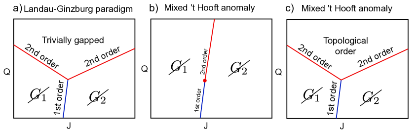
Phase transitions and symmetries have a close connection. When a system has a particular symmetry, it can typically be driven into a phase where the symmetry is spontaneously broken, or restored. According to the Landau-Ginzburg paradigm, the effective description of this transition can be written as an effective quantum field theory of the order parameter, and thus, since any two systems with the same symmetries can be captured by such an effective description, all of such transitions are universal. According to this lore, a transition with a symmetry group of the form from a phase where the symmetry breaking pattern is to a phase where the symmetry breaking pattern is must generically be of 1st order. The reason is that, unless there is some fine tuning, there is no reason for both order parameters to go to zero at the same time. As a consequence the system is typically multi-critical – see Fig. 1.
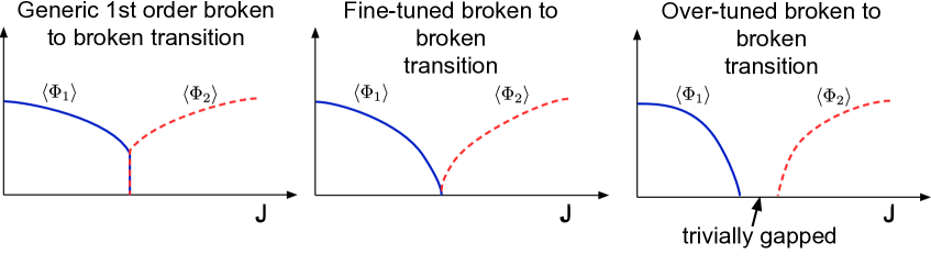
However, if the symmetry group has a mixed ‘t Hooft anomaly111A mixed ’t Hooft anomaly can be thought of as breaking of the symmetry if gauge fields for the symmetry are introduced. between the symmetries and , the Landau-Ginzburg paradigm breaks down. A mixed ’t Hooft anomaly requires that either or is spontaneously broken, and so the trivially gapped phase is impossible, i.e., the scenario in the far left of Fig. 1 cannot happen. Thus it is plausible that a generic 2nd order order-to-order transition can happen in systems with a mixed ’t Hooft anomaly (see Fig. 2b). However, also another gapped phase could emerge, potentially developing some kind of topological order.
The most prominent system which was suggested to have a generic 2nd order transition is that of a 2+1d spin-1/2 anti-ferromagnet, going from a Néel to the VBS phase, for which a generic 2nd order transition was proposed to exist [1]. The Néel phase is a phase where the spin symmetry222The symmetry of spin is , not because the spin operator is an vector, and there exists no operator which transforms in an representation which is not in . is spontaneously broken to , while the VBS phase is a phase where two neighboring spins combine into a singlet dimer and spontaneously break the lattice symmetries. The symmetry breaking pattern for the VBS phase depends on the details of the lattice, but for a square lattice the breaking leaves vacua related by the group generated by the 90-degree lattice rotations.
The basic premise is that the spin model in question is effectively described by scalar QED in 3d, with a gauge-charge unity scalar doublet . The model has an flavor symmetry rotating the scalars333Note that because the scalar doublet carries gauge charge one, the action of the center of is given by , which is a gauge symmetry, not a global symmetry. Hence the global symmetry is , not . , i.e., , consistent with the spin-symmetry of the spin-1/2 anti-ferromagnet. Further, since the system has an abelian gauge field , it also has a conserved current , where is the totally anti-symmetric tensor. The validity of is a statement that there exists a -magnetic symmetry, the so-called magnetic symmetry, which is not a symmetry of the spin-1/2 antiferromagnet. This symmetry is broken by the presence of magnetic monopole operators in the theory. However, a relevant symmetry is a -symmetry of lattice rotations by 90 degrees, which in the infrared theory transmutes444It may come as a surprise that the spatial lattice symmetry has anything to do with the internal symmetry of the effective model. The statement is that an operator which preserves the symmetry of the lattice, but breaks the symmetry completely has to have a large momentum, of the order of the inverse lattice system size, and as such decouples in the thermodynamic limit. Such symmetries are dubbed emanent symmetries [2]. into the -subgroup of the -magnetic symmetry. Hence an effective theory of the spin-1/2 system is the 2-scalar QED with charge monopoles, preserving the -subgroup of -magnetic.
The presence of a generic 2nd order transition requires that the charge- monopole operators are irrelevant at the corresponding conformal fixed point555The fixed point is sometimes called deconfined critical point (DCP)., which is indeed the case in the generalizations of the model when is large [3, 1]. However, the generic 2nd order nature has a controversial history (see [4] for a recent paper). Recent results on the spin-1/2 models seem to indicate that the scenario Fig. 2c) is realized. However, in spin systems at least the -magentic symmetry needs to emerge666It is believed that perhaps even symmetry emerges at the (multi-)critical point. See [4] and references therein.. In this work instead, we consider the lattice formulation of the 2-scalar QED model with an exact magnetic symmetry777Note that in [5] Fermionic in the same universality class with the exact symmetry was also considered. which is possible using the modified Villain formalism888We would like to point out some interesting development in the direction of the Villainized modal of non-abelian gauge theory [6, 7]. [8, 9, 10, 11, 12, 13, 14, 15, 16, 17, 18]. Preliminary results presented here seem to indicate a 2nd order phase transition, but further simulations on larger lattices are needed to reliably resolve the nature of the transition.
2 Definition of the model
The system we study is defined on a 3d lattice with volume . All fields obey periodic boundary conditions. The partition function depends on two couplings, the inverse gauge coupling and the matter coupling ,
| (1) |
The gauge field degrees of freedom are assigned to the links of the lattice, with the corresponding path integral measure given by . The Boltzmann factor for the gauge degrees of freedom is given by
| (2) | |||||
| (3) |
where is the sum over all configurations of the plaquette-based Villain variables , defined as , and denotes the exterior derivative of the gauge fields. The Villain variables are subject to constraints that in (2) are implemented with a product of Kronecker deltas (here denoted as ) that enforce
| (4) |
which implies the absence of monopoles. The spin degrees of freedom are given by
| (5) |
The path integral measure is again a product measure, . Finally, the action for the spin degrees of freedom is
| (6) | |||
3 Observables
For our analysis we use two order parameters. The spin order parameter (magnetization) is defined as, ( is the vector of Pauli matrices)
| (7) |
with a non-zero expectation value of signalling the breaking of SO(3). Our second order parameter is the total net winding number of closed monopole loops on the dual lattice,
| (8) |
When viewed on the dual lattice, where we denote sites as and the dual Villain variables as , it is obvious that the sum turns into , which corresponds to the total net flux of through the dual 2-3 plane at (thus the normalization with to obtain an intensive quantity). On the dual lattice the constraint (4) turns into the zero divergence condition , which implies flux conservation of the . As a consequence equals the total net winding number around the periodic 1-direction, and similarly the other two sums correspond to winding around the 2- and 3-directions. The observable thus gives the absolute value of the net flux density averaged over all three directions of the dual lattice. Note that the constraint (4) forbids isolated monopoles or anti-monopoles, but a non-zero winding number of closed monopole loops on the dual lattice is admissible. This is what is measuring.
For locating the critical point and a first analysis of its universality class we furthermore study the susceptibility of and the corresponding Binder cumulant ,
| (9) |
where for later use we also defined the Binder ratios and . Here we have a 3-component vector as order parameter such that the normalization factor in the Binder cumulant is .
4 Numerical simulation
So far only local updates are implemented for all degrees of freedom, but a more advanced update strategy could use worms for the Villain variables . For the angles we use proposal values and in case of add in oder to project back into (periodic completion). The update of the angles is done in the same way, and in both cases the proposal is accepted or rejected with a Metropolis step. For the angles we use proposal values and in case of we reject the proposal and go to the next spin (hard boundary rejection). If the proposal is admissible, a Metropolis step is used to accept or reject the proposal. For the update of the gauge fields we again use and project back into by adding in case .
In the update of the Villain variables the constraints (4) must be taken into account. For this purpose we use two types of updates: 1.) updates where we simultaneously change the Villain variables on four plaquettes that share a common link (i.e., a plaquette on the dual lattice), and 2.) updates where we change the Villain variables on stacks of plaquettes. For the dual plaquette update we choose randomly and for the Villain variables on plaquettes that share the link offer the change which we accept or reject with a Metropolis step. In a similar way we change the Villain variables on plaquettes that share links in the 2- and 3-directions. It is easy to see that with the correct distribution of signs in the changes the constraints (4) remain intact. In order to obtain an ergodic update, the dual plaquette update has to be combined with the update of Villain variables on stacks of plaquettes, which correspond to winding loops on the dual lattice. For example we offer the collective change of Villain variables , where again . Again the proposal is accepted or rejected with a Metropolis step.
In this preliminary study we work at an inverse gauge coupling of with lattice extents of and . We typically use ensembles with configurations ( for the Binder cumulants) separated by 50 blocks of updates, where each block combines 5 sweeps through all d.o.f.s and with both, 5 sweeps of local cube updates and 5 dual winding sweeps for the . We equilibrate the system with block updates. All errors we show are statistical errors determined with a jackknife analysis combined with blocking of the data.
5 Results
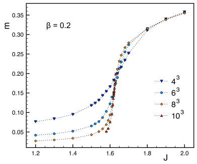
We begin the presentation of our results with the discussion of the order parameters. In the lhs. plot of Fig. 3 we show the magnetization density as a function of for different volumes. It is obvious that at a critical value of the system develops a magnetization and changes from a symmetric phase into a phase where SO(3) is broken.
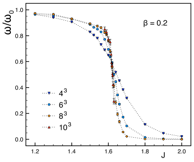
In the rhs. plot of Fig. 3 we show the winding number where the normalization is done with , i.e., the winding number density evaluated at vanishing coupling . Here we observe that at the same critical value the winding number of monopole lines around the periodic boundary conditions drops to zero, while for it is finite and monopoles could propagate. We also analyzed the correlator of a monopole-antimonopole pair which we can generate at the endpoints of a string of dual links along which the corresponding Villain variables are changed by , thus explicitly violating the constraint (4) with a source term. We find that at the correlator abruptly changes its behavior towards fast decay. A more detailed analysis of this behavior is in preparation, but the qualitative study we did so far indicates that the drop of the winding number observed in the rhs. plot of Fig. 3 is due to a change of the monopole-antimonopole correlator at .
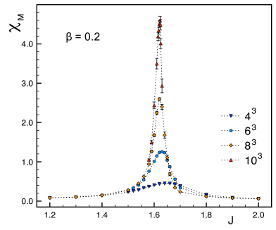
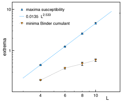
To further characterize the transition at we study the susceptibility , which we show as a function of in the lhs. plot of Fig. 4. The susceptibilities develop pronounced peaks that grow with the volume, as is characteristic for a phase transition. In the rhs. plot we show with blue triangles the maxima of as a function of in a log-log plot. The growth is well described by a power law with an exponent , which is smaller than the dimension , thus indicating a continuous transition ( and are the critical exponents for susceptibility and correlation length).
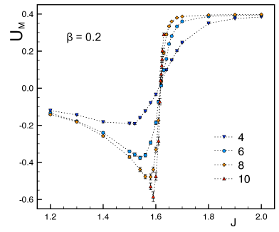
We finally come to the analysis of the Binder cumulant. In the lhs. plot of Fig. 6 we show the Binder cumulant as defined in (9) as a function of . The Binder cumulant shows the expected crossing of the curves for different volumes at the critical value . However, the curves also develop minima below which need to be understood, since minima that grow with the volume are an indication for first order behavior. In the log-log plot in the rhs. of Fig. 4 we also show the size of the minima we observe in the Binder cumulant. Obviously we do not see volume scaling, indicating that the minima in the Binder cumulant do not signify a first order transition.
We remark, that we also conducted a small study in the 3d O(4) model, which our system reduces to when the gauge fields are omitted. In the ungauged O(4) model one can directly use the spin expectation value as order parameter (which in our model is not a gauge invariant observable), and based on that analysis it is well established that the O(4) model undergoes a single continuous transition. However, it is possible to study this transition also with our order parameter as defined in (7) and also in the O(4) model the corresponding Binder cumulants develop the same minima as observed here. The deeper reason for this behavior is that is a monomial of order 8 in the spin degrees of freedom, leading to additional minima in the observable, which, however, are not linked to some first order behavior.
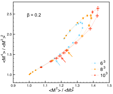
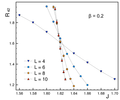
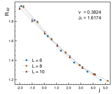
Yet another evidence that the transition we observe at is continuous is presented in the rhs. plot of Fig. 6, where we show the Binder ratios versus . According to the finite size scaling ansatz for continuous transitions, both these ratios should behave like universal functions , , where and is again the critical exponent of the correlation length. Thus for a continuous transition the curves for the different volumes should fall on top of each other in the scaling region (arrows in the plot), and this is what we indeed observe.
To complete our analysis by exploiting the finite size scaling relation for the Binder cumulant and show as a function of in the rhs. plot of Fig. 6 (the lhs. plot shows the raw data as a function of ). When choosing and we find the optimal collapse of the data. Repeating the collapse with the Binder cumulant , we find and .
However, we remark that is inconsistent with the conformal bootstrap constraint for having a critical, rather than multi-critical, point (see [19] Appendix C). While the analysis is still preliminary, this indicates that the transition is likely weakly first order, passing near a multi-critical fixed point, supporting scenario Fig. 1c. Only simulations on larger volumes will resolve this issue.
Acknowledgments
We thank Fakher Assad for discussions at SIGN-25. TS is supported by the University Research Fellowship of the Royal Society of London and, in part, by the STFC grant number ST/T000708/1.
References
- [1] T. Senthil, A. Vishwanath, L. Balents, S. Sachdev and M. P. A. Fisher, Deconfined Quantum Critical Points, Science 303 (2004) 1490, [cond-mat/0311326].
- [2] M. Cheng and N. Seiberg, Lieb-Schultz-Mattis, Luttinger, and ’t Hooft - anomaly matching in lattice systems, SciPost Phys. 15 (2023) 051, [2211.12543].
- [3] G. Murthy and S. Sachdev, Action of Hedgehog Instantons in the Disordered Phase of the (2+1)-dimensional Model, Nucl. Phys. B 344 (1990) 557.
- [4] J. Takahashi, H. Shao, B. Zhao, W. Guo and A. W. Sandvik, SO(5) multicriticality in two-dimensional quantum magnets, 2405.06607.
- [5] Y. Liu, Z. Wang, T. Sato, M. Hohenadler, C. Wang, W. Guo et al., Superconductivity from the Condensation of Topological Defects in a Quantum Spin-Hall Insulator, Nature Commun. 10 (2019) 2658, [1811.02583].
- [6] J.-Y. Chen, Instanton Density Operator in Lattice QCD from Higher Category Theory, 2406.06673.
- [7] P. Zhang and J.-Y. Chen, An Explicit Categorical Construction of Instanton Density in Lattice Yang-Mills Theory, 2411.07195.
- [8] T. Sulejmanpasic and C. Gattringer, Abelian gauge theories on the lattice: -Terms and compact gauge theory with(out) monopoles, Nucl. Phys. B 943 (2019) 114616, [1901.02637].
- [9] M. Anosova, C. Gattringer, D. Göschl, T. Sulejmanpasic and P. Törek, Topological terms in abelian lattice field theories, PoS LATTICE2019 (2019) 082, [1912.11685].
- [10] P. Gorantla, H. T. Lam, N. Seiberg and S.-H. Shao, A modified Villain formulation of fractons and other exotic theories, J. Math. Phys. 62 (2021) 102301, [2103.01257].
- [11] M. Anosova, C. Gattringer and T. Sulejmanpasic, Self-dual U(1) lattice field theory with a -term, JHEP 04 (2022) 120, [2201.09468].
- [12] M. Anosova, C. Gattringer, N. Iqbal and T. Sulejmanpasic, Phase structure of self-dual lattice gauge theories in 4d, JHEP 06 (2022) 149, [2203.14774].
- [13] L. Fazza and T. Sulejmanpasic, Lattice quantum Villain Hamiltonians: compact scalars, U(1) gauge theories, fracton models and quantum Ising model dualities, JHEP 05 (2023) 017, [2211.13047].
- [14] T. Jacobson and T. Sulejmanpasic, Modified Villain formulation of Abelian Chern-Simons theory, Phys. Rev. D 107 (2023) 125017, [2303.06160].
- [15] M. Nguyen, T. Sulejmanpasic and M. Ünsal, Phases of theories with 1-form symmetry and the roles of center vortices and magnetic monopoles, 2401.04800.
- [16] T. Jacobson and T. Sulejmanpasic, Canonical quantization of lattice Chern-Simons theory, JHEP 11 (2024) 087, [2401.09597].
- [17] Z.-A. Xu and J.-Y. Chen, Lattice Chern-Simons-Maxwell Theory and its Chirality, 2410.11034.
- [18] C. Peng, M. C. Diamantini, L. Funcke, S. M. A. Hassan, K. Jansen, S. Kühn et al., Hamiltonian Lattice Formulation of Compact Maxwell-Chern-Simons Theory, 2407.20225.
- [19] Y. Nakayama and T. Ohtsuki, Conformal Bootstrap Dashing Hopes of Emergent Symmetry, Phys. Rev. Lett. 117 (2016) 131601, [1602.07295].