The cosmic optical background intensity from decaying sterile neutrinos via magnetic dipole moment

Abstract

NASA’s New Horizon observations yielded the most accurate measurement of the cosmic optical background (COB) intensity. The reported COB flux is $16.37\pm 1.47$ $\mathrm{nW/m^{2}/sr}$ at a pivot wavelength $\lambda_{piv}=0.608\,\mu\mathrm{m}$ observed in the range $0.4\,\mu\mathrm{m}\lesssim\lambda\lesssim 0.9\,\mu\mathrm{m}$. After subtracting the measured intensity from the deep Hubble space telescope count, an anomalous excess flux $8.06\pm 1.92\leavevmode\nobreak\ \mathrm{nW/m^{2}/sr}$ has been found. This observation could hint toward decaying dark matter producing photons. In this work, we have considered sterile neutrinos of the keV scale as well as the eV scale decaying via sterile-to-sterile transition magnetic dipole moment and active-to-sterile transition magnetic dipole moment, respectively, to explain anomalous flux. The sterile neutrinos with a mass of $\mathcal{O}(\rm keV)$ with transition magnetic moment in the range $3\times 10^{-14}\,\mu_{B}-10^{-13}\,\mu_{B}$, and mass of $\mathcal{O}(\rm eV)$ with transition magnetic moment in the range $3.33\times 10^{-13}\,\mu_{B}-10^{-12}\,\mu_{B}$ can successfully account for the observed anomalous intensity.

I Introduction

Line-intensity mapping (LIM) is an observational method for extragalactic astronomy and cosmology that measures the integrated intensity of spectral lines emitted from galaxies and the intergalactic medium at a specific observed frequency Kovetz et al. (2017, 2020). Since LIM experiments capture information from all incoming photons, they have the potential to detect electromagnetic radiation produced by dark matter decays directly. For instance, in Ref. Grin et al. (2007), authors have derived a stringent upper bound on the axion-photon coupling strength by searching for optical line emission produced from decaying axions. In Ref. Gong et al. (2016), authors have shown that photons produced from decaying axions with eV mass can explain the anisotropy of near-IR extragalactic background light. In Ref. Creque-Sarbinowski and Kamionkowski (2018), authors have proposed that LIM experiments can detect photons produced from decaying and annihilating dark matter particles.

Measuring the extragalactic background light in the optical band is a difficult task. The primary reason is mitigating the overwhelming foreground, which requires accurate modelling and well-calibrated instruments Bernal et al. (2022). In Ref. Zemcov et al. (2017a), authors have suggested observing such radiations in the optical spectrum—the cosmic optical background (COB) is possible if one can eliminate the foreground radiations, primarily solar in nature. Recently, the Long Range Reconnaissance Imager (LORRI) mounted on NASA New Horizons spacecraft operating at a distance $51.3\,\rm AU$ measured the COB photon flux intensity in the wavelength range $0.4\,\mu\mathrm{m}\lesssim\lambda\lesssim 0.9\,\mu\mathrm{m}$ $(\sim 1.3\leavevmode\nobreak\ \rm eV-3\leavevmode\nobreak\ \,\rm eV)$ Zemcov et al. (2017b); Lauer et al. (2021a, b). This measurement yields an intensity of $16.37\pm 1.47$ $\mathrm{nW/m^{2}/sr}$, which is greater than twice the intensity measured by deep Hubble Space Telescope (HST) with $>4\sigma$ significance Lauer et al. (2021b). Earlier, it was suggested that the COB only comprises the integrated light of external galaxies presently known from deep HST counts Lauer et al. (2021b). Therefore, after subtracting the contribution from integrated galaxy light (IGL), which is equal to $8.31\pm 1.24$ $\mathrm{nW/m^{2}/sr}$, an anomalous excess flux of $8.06\pm 1.92\leavevmode\nobreak\ \mathrm{nW/m^{2}/sr}$ at a pivot wavelength $\lambda_{\rm{pivot}}=0.608\,\mu\rm m\,(\sim 2\,\rm eV)$ was found Lauer et al. (2021b). There are possible astrophysical explanations for this anomaly, such as unaccounted faint galaxies in the deep HST counts Conselice et al. (2016), infrared background from high redshifted accreting direct collapse black holes Yue et al. (2013), faint sources within extended halos Cooray (2016); Zemcov et al. (2017a); Matsumoto and Tsumura (2019).

This anomalous photon excess may indicate the presence of physics beyond the Standard Model. Various studies have explored possible explanations, such as photons emitted from decaying axions with masses in the range of $\sim 5\rm eV-25\rm eV$ Bernal et al. (2022); Nakayama and Yin (2022); Carenza et al. (2023). Additionally, decaying sterile neutrinos could produce a similar photon signal through their decay into photons and neutrinos. Short-baseline neutrino experiments have hinted at the existence of additional neutrinos, and numerous studies have investigated sterile neutrinos as a potential dark matter candidate. Therefore, it is crucial to examine this photon excess in the context of sterile neutrinos, as it could provide new insights into dark matter. Motivated by these possibilities, we investigate sterile neutrinos as a potential source of the observed photon excess. A sizable transition magnetic dipole moment could enhance photon production from sterile neutrinos, making this anomaly a valuable probe of new physics in the neutrino sector. The transition magnetic dipole moment of sterile neutrino allows it to interact with standard model particles such as active neutrinos, gauge bosons, and photons Ge and Pasquini (2023a). In particle physics, the transition magnetic dipole moment denotes that a sterile neutrino possesses a non-zero intrinsic magnetic orientation, allowing it to interact with external magnetic fields Ge and Pasquini (2023b). There have been several studies on the phenomenological implications of active-to-active and active-to-sterile neutrino transition magnetic moments, particularly for small neutrino masses, using both effective field theory approaches and models beyond the Standard Model Voloshin (1987); Barbieri and Mohapatra (1989); Babu et al. (2020, 2021); Schwetz et al. (2021). Many experiments have placed upper limits on these magnetic moments, with constraints on sterile-to-sterile transition magnetic moments being relatively weaker, especially at smaller mass scales. The sterile-to-sterile transition magnetic dipole moment for neutrinos in the GeV mass range has been studied in the context of long-lived particle (LLP) searches in various experiments, such as AL3X, ANUBIS, CODEX-b, FACET, MAPP, and FASER/FASER$\nu$ Barducci et al. (2023); Günther et al. (2024). This research opens new opportunities for LLP searches at the Large Hadron Collider (LHC) Beltrán et al. (2024). Additionally, measurements from COB provide a complementary method for constraining transition magnetic moments.

In our work, we focus on the keV mass scale for sterile neutrinos, as they are considered a viable dark matter candidate, as well as we have considered the eV mass scale of decaying sterile neutrinos. Rather than considering a specific model, we adopt an effective field theory approach Beltrán et al. (2024), which makes our analysis more general and less dependent on particular model assumptions. Anomalies observed in short-baseline neutrino experiments, such as MiniBooNE Aguilar-Arevalo et al. (2021, 2018) and LSND Aguilar et al. (2001), have sparked significant interest in the possibility of eV-scale sterile neutrinos, which have been extensively studied in the literature. Motivated by these scenarios, we investigate the potential role of eV-scale sterile neutrinos in explaining the COB excess.

The paper is organised as follows. In Section II, we discuss the radiative decay process of sterile neutrinos through the sterile-to-sterile and sterile-to-active transition magnetic dipole moment in the low-energy effective field theory. In Section III, we derive the mean specific intensity for the keV mass range of decaying sterile neutrinos to explain the COB anomaly. In Section IV, we have analysed our results by determining the minimal required magnetic dipole moment for sterile-to-sterile and active-to-sterile transition magnetic dipole moment and the existing limits on it. In Section V, we present our conclusions with an outlook for future works.

II Radiative Decay of Sterile Neutrino through Transition Magnetic Dipole Moment

We consider Standard model augmented with sterile neutrinos in effective field theory approach. Assuming sterile neutrino mass scale well below the electroweak scale, we can write the effective Lagrangian contributes to the magnetic moment of neutrino sector:

$$\mathcal{L}_{N_{R}LEFT}\supset d_{\rm NN\gamma}^{ij}\mathcal{O}_{\rm NN\gamma}^{ij}+d_{\nu N\gamma}^{\beta i}\mathcal{O}_{\nu N\gamma}^{\beta i}+\text{h.c.}\,,$$ (1)

where $d_{\rm NN\gamma}$ represents the sterile-to-sterile transition magnetic dipole moment and $d_{\rm\nu N\gamma}$ denotes the active-to-sterile transition magnetic dipole moment. The term $\mathcal{O}_{\rm NN\gamma}^{ij}=(\bar{N}_{Ri}^{c}\sigma_{\mu\nu}N_{Rj})F^{\mu\nu}$, $\mathcal{O}_{\nu N\gamma}^{\alpha i}=(\bar{\nu}_{L\alpha}^{c}\sigma_{\mu\nu}N_{Ri})F^{\mu\nu}$ represent the effective field operators, where $F^{\mu\nu}$ is the electromagnetic field strength tensor.

The electric and magnetic field off-diagonal non-zero dipole moment components give rise to radiative decay through two different sterile states. Therefore, in this radiative decay process ($m_{1}\rightarrow m_{2}+\gamma$), the decay width of sterile neutrino can be written as Atre et al. (2009); Bondarenko et al. (2018); Balantekin and Vassh (2014)

$$\Gamma_{m_{1}}(m_{1}\rightarrow m_{2}+\gamma)=\frac{2|d_{\rm NN\gamma}|^{2}}{\pi}m_{1}^{3}\left(1-\frac{m_{2}^{2}}{m_{1}^{2}}\right)^{3}.$$ (2)

By defining $\delta=1-\frac{m_{2}}{m_{1}}$, which represents the mass splitting between two eigenstates of sterile neutrino, we can rewrite Eq. (2) as

$$\Gamma_{m_{1}}(m_{1}\rightarrow m_{2}+\gamma)=\frac{2|d_{\rm NN\gamma}|^{2}}{\pi}m_{1}^{3}\left(2-\delta\right)^{3}\delta^{3},$$ (3)

From Eq. (3), we can derive the sterile-to-sterile transition magnetic dipole moment $d_{\rm NN\gamma}$.

There are several experimental upper bounds on the neutrino magnetic moment. Recent studies of the NOMAND neutrino detector at CERN put constraints on the active-to-sterile transition magnetic dipole moment $d_{\rm\nu N\gamma}\lesssim(10^{-6}-10^{-9})\mu_{B}$ Gninenko and Krasnikov (1999). In an anti-neutrino electron scattering experiment, by examining the electron recoil spectra, it was found that active-to-sterile transition magnetic dipole moment $d_{\rm\nu N\gamma}\lesssim 10^{-9}\mu_{B}$ Derbin et al. (1993). The Super-Kamiokande experiment put an upper bound limit on active-to-sterile transition magnetic dipole moment $d_{\rm\nu N\gamma}\lesssim 1.1\times 10^{-10}\mu_{B}$ Liu et al. (2004), and the Borexino collaboration put the upper bound limit at $90\%$ confidence level as $5.4\times 10^{-11}\mu_{B}$ Agostini et al. (2017); Arpesella et al. (2008). MUNU collaboration has found the upper bound on active-to-sterile transition magnetic dipole moment $d_{\rm\nu N\gamma}\lesssim 9.0\times 10^{-11}\mu_{B}$ Babu et al. (2020), whereas TEXONO collaboration has obtained this active-to-sterile transition magnetic dipole moment upper bound limit $d_{\rm\nu N\gamma}\lesssim 7.4\times 10^{-11}\mu_{B}$ Balantekin and Vassh (2014). The Planck+BAO put the constraint on the active-to-sterile transition magnetic dipole moment, and it varies from $3.7\times 10^{-11}\mu_{B}$ to $9.1\times 10^{-12}\mu_{B}$ Carenza et al. (2024). Recent studies analysing the cooling of red giant stars have found an upper limit on active-to-sterile transition magnetic dipole moment $d_{\rm\nu N\gamma}\lesssim 1.2\times 10^{-12}\mu_{B}$ Capozzi and Raffelt (2020). The anomalous stellar cooling due to plasmon decay has been found an upper limit on active-to-sterile transition magnetic dipole moment $d_{\rm\nu N\gamma}$ is $d_{\rm\nu N\gamma}\lesssim 3\times 10^{-12}\mu_{B}$ Alexander (2016).

III Mean specific intensity of decaying sterile neutrinos

Consider a radiative decaying particle of rest mass $m_{\chi}$ represented as $\chi\to\gamma+\xi$, where $\gamma$ and $\xi$ represent a photon and another particle, respectively. The wavelength of the photon produced in the rest frame of $\chi$ is Chen and Kamionkowski (2004); Bernal et al. (2021)

$$\lambda_{e}=\frac{hc}{m_{\chi}c^{2}}\times\frac{2}{\left(1-m_{\xi}^{2}/m_{\chi}^{2}\right)}$$ (4)

where $h$ and $c$ are the Planck’s constant and the speed of light in vacuum, respectively. We define the second term on the right-hand side of Eq. (4) as $x^{-1}=\frac{2}{\left(1-m_{\xi}^{2}/m_{\chi}^{2}\right)}$. We note that for a two-photon decay process, $x=1/2$. The wavelength of photon produced from a particle decaying at redshift $z$ will be observed today as $\lambda_{obs}=(1+z)\lambda_{e}$. If these photons are not absorbed by the intergalactic gas along the light of sight, then they will be observed today as the extra-galactic background lights.

The redshift dependence of the energy density of decaying dark matter particles is given by $\rho_{\chi}(t)=\rho_{\chi}(0)(1+z)^{3}\mathrm{e}^{-\Gamma_{\chi}t_{\rm U}}$, where $t_{\rm U}\sim 10^{18}\,\rm sec$ is the age of the universe, $\Gamma_{\chi}$ represents the decay rate, and $\rho_{\chi}(0)$ is the dark matter energy density today. If $\Gamma_{\chi}$ of decaying dark matter particle is such that $\Gamma_{\chi}t_{\rm U}\lesssim 10^{-2}$, we can then consider $e^{-\Gamma_{\chi}t_{\rm U}}\approx 1$. Later in this section, we have shown that the decay rate considered in this work justifies this approximation. The specific intensity of the photons $I_{\nu}$ observed at frequency $\nu_{\rm obs}$ today is given by Creque-Sarbinowski and Kamionkowski (2018)

$$I_{\nu}=\dfrac{1}{4\pi}\int_{0}^{\infty}{dz}\dfrac{c}{H(z)}\dfrac{\epsilon_{\nu_{\rm obs}}(z)}{(1+z)^{4}},$$ (5)

where $\epsilon_{\nu_{\rm obs}}$ is the specific luminosity density and $H(z)$ is the Hubble parameter. For a Dirac delta decaying profile, $\epsilon_{\nu_{\rm obs}}$ is expressed as Chen and Kamionkowski (2004); Creque-Sarbinowski and Kamionkowski (2018)

$$\epsilon_{\nu_{\rm obs}}(z)=h\mathrm{N}_{\gamma}\Gamma_{\chi}\mathrm{n}_{\chi}(z)\mathrm{E}_{\gamma}\,\delta(\rm E-E_{\gamma}),$$ (6)

where $\rm N_{\gamma}$ and $\rm n_{\chi}(z)$ represent the number of photons produced and the number density of the decaying particles. On solving Eq. (5) for the aforementioned $\epsilon_{\nu_{\rm obs}}$ and using the relation, $I_{\lambda}=I_{\nu}\left|\mathrm{d\nu}/\mathrm{d\lambda}\right|$ we calculate the mean specific intensity per observed wavelength as

$$I_{\lambda}=\frac{c}{4\pi}\frac{\Omega_{\chi,0}\rho_{c}\Gamma_{\chi}}{\lambda_{\rm obs}(1+z)\text{H}(z)m_{\chi}}\leavevmode\nobreak\ \frac{hc}{\lambda_{e}}N_{\gamma},$$ (7)

where $\Omega_{\chi,0}$ represents the present-day dark matter density parameter and $\rho_{c}$ is the critical density.

In this work, we consider a decaying sterile neutrino of mass $m_{1}$ to produce a photon and another sterile neutrino of mass compared to $m_{2}$. In this case, the term $hc/\lambda_{e}$ in Eq. (7) can be replaced with $x\,m_{1}c^{2}$. Considering both $m_{1}$ and $m_{2}$ are of $\mathcal{O}(\rm keV)$, we can approximate $m_{1}+m_{2}\sim 2m_{1}$. The photon’s energy produced from this process becomes $E_{\gamma}=m_{1}-m_{2}$. From hereinafter, we define $m_{1}-m_{2}=\Delta m$. Consequently, the term $x$ mentioned earlier will be $\Delta m/m_{1}$. On substituting all the terms as mentioned above in Eq. (7), we rewrite the equation as

$$I_{\lambda}=\frac{c}{4\pi}\frac{{\Omega_{\chi,0}}{\rho_{c}}{c^{2}}\Gamma_{m_{1}}}{\lambda_{obs}(1+z)H(z)}\leavevmode\nobreak\ \frac{\Delta m}{m_{1}}.$$ (8)

From the above equation, we can observe that $I_{\lambda}$ is directly proportional to the decay rate and the energy of the released photon. However, it is inversely related to the mass of the decaying particle and decays down over redshifts due to the expansion of the Universe.

IV Results and Discussions

In the previous section, we discussed that the photon production intensity mediated by radiative decays is directly linked to the neutrino magnetic moment. Here, we investigate the COB excess and analyze it within the framework of the neutrino magnetic moment. Specifically, we investigate three possible scenarios: sterile-sterile, sterile-active, and active-active neutrino magnetic moments.

IV.1 Sterile to sterile neutrino decay

In this section, we calculate the required decay rate and the transition magnetic moment to explain the COB excess. We consider the keV mass range sterile neutrino as a dark matter candidate, which decays into another sterile neutrino and photon through the radiative decay process. We note that the sterile neutrinos with mass $<0.4\,\rm keV$ are excluded as a dark matter candidate by a conservative application of Tremaine-Gunn bound Abazajian and Koushiappas (2006). Now, to calculate $I_{\lambda}$ required to explain the COB excess, we need to determine the energy of photons $(\Delta m)$, as shown in Eq. (8). The LORRI observation reported flux of photons at pivot wavelength $0.608\,\mu m\,(\sim 2\,\rm eV)$ Lauer et al. (2021b). Therefore, $\Delta m$ should be in the range $2\,\rm eV-10\,\rm eV$, such that LORRI’s band could observe these redshifting photons today. We restrict the energies of photons in this range, as the photons produced at $z\gtrsim 4$ will get absorbed by the intergalactic gas medium Madau (1995); Inoue et al. (2014). For a fixed $\Gamma_{m_{1}}=10^{-21}\,\rm sec^{-1}$ and $m_{1}=1\,\rm keV$, we present $I_{\lambda}$ in Fig. 1. In this figure, the vertical lines at lower wavelengths represent $\lambda_{e}$ of photons observed today. The green-shaded region represents $I_{\lambda}$ calculated from the LORRI camera for radiative decaying dark matter, which can be found in Ref. Bernal et al. (2021). We then vary $\Gamma_{m_{1}}$ in the range $10^{-21}\text{sec}^{-1}-10^{-22}\text{sec}^{-1}$, while fixing $m_{1}=1\,\rm keV$ and the total intensity $(I)$ to be $8.06\pm 1.92\,\rm nW/m^{2}/sr$ as reported in LORRI Lauer et al. (2021b). The corresponding $I_{\lambda}$ is shown in Fig. 1. We observe that the intensity curves are clumped at the lower $\lambda_{\rm obs}$ values. This suggests that the produced photons with energy $\Delta m$ for the aforementioned $m_{1}$ and $\Gamma_{m_{1}}$ originate from higher redshifts. From Eq. (8), we can observe that high energetic photons originating at higher redshifts require smaller $\Gamma_{m_{1}}$. Therefore, a sterile neutrino with a large decay width is required to produce less energetic photons in order to explain the COB excess intensity. In the next section, we present the minimum required $\Gamma_{m_{1}}\rm$, and hence the $d_{\rm NN\gamma}\rm$, to explain the COB excess intensity for different $m_{1}$ values.

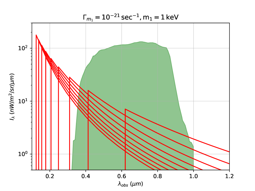
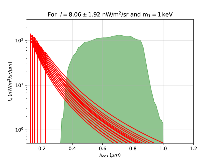
Figure 1: (a) illustrates the variation in specific intensity $I_{\lambda}$ with respect to $\lambda_{\rm obs}$, for $\Gamma_{m_{1}}=10^{-21}\,\text{sec}^{-1}$ and $m_{1}=1\,\rm keV$. (b) The variations in $I_{\lambda}$ contributing to LORRI’s reported COB excess intensity, that is, the total intensity is equal to $8.06\pm 1.92\,\rm nW/m^{2}/sr$, for $\Gamma_{m_{1}}\sim(10^{-22}-10^{-21})\,\text{sec}^{-1}$ and $m_{1}=1\,\rm keV$. The green-shaded area illustrates the responsivity curve of LORRI for each detected wavelength, depicted with an unnormalized shape.

In Fig. (2), we plot the required minimum decay width for different masses— shown in the red solid line. We find that, for sterile neutrinos of mass $m_{1}=1\,\rm keV$, the minimum required decay rate is $\Gamma_{m_{1}}\sim 6\times 10^{-22}\,\rm sec^{-1}$. The decay width of the sterile neutrino increases as we increase the mass. This can be analysed from the fact that $I_{\lambda}\propto\Gamma_{m_{1}}/m_{1}$— shown in Eq. (8). We restrict our analysis to $1\leq m_{1}/\rm keV\leq 20$ because a further increase in $m_{1}$ requires an increase in $\Gamma_{m_{1}}$. For instance, the required $\Gamma_{m_{1}}$ for $m_{1}=20\,\rm keV$ reached a value $\sim 10^{-20}\,\rm sec^{-1}$. Thus, for $m_{1}\gtrsim 20\,\rm keV$, the corresponding $\Gamma_{m_{1}}$ become comparable to $\sim t^{-1}_{\rm U}$ which requires a consideration of variation in the dark matter density— as mentioned in section (III).

We then plot the minimum values of $d_{\rm NN\gamma}$ derived from the $\Gamma_{m_{1}}$ required to explain the COB excess— shown in the green solid line. We find that under the conditions $m_{1}+m_{2}\sim 2m_{1}$ and $m_{1}-m_{2}=\Delta m$, the decay width Eq. 2 become $16|d_{\rm NN\gamma}|^{2}\,\Delta m^{3}/\pi$. As mentioned earlier, $\Delta m$ takes values of $2\,\rm eV-10\,\rm eV$ for the observed flux of photons. Therefore, to calculate minimum $d_{\rm NN\gamma}$, we consider minimum values of $\Gamma_{m_{1}}$ for corresponding $m_{1}$ values while fixing $\Delta m=10\,\rm eV$. We find that the transition magnetic moment $d_{\rm NN\gamma}/\rm eV^{-1}$ takes values of $\left(\sim 8.8\times 10^{-21}-3.8\times 10^{-20}\right)$ for $m_{1}$ in $1\,\rm keV-20\,\rm keV$, respectively, as shown in the green solid line of Fig. (2). In the unit of Bohr magneton $(\mu_{B}\sim 3\times 10^{-7}\,\rm eV^{-1})$, $d_{\rm NN\gamma}$ takes values of $(3\times 10^{-14}-10^{-13})\mu_{B}$. In the next section, we discuss the possibility of explaining the COB excess anomaly from decaying sterile neutrino via the sterile-to-active transition magnetic dipole moment.

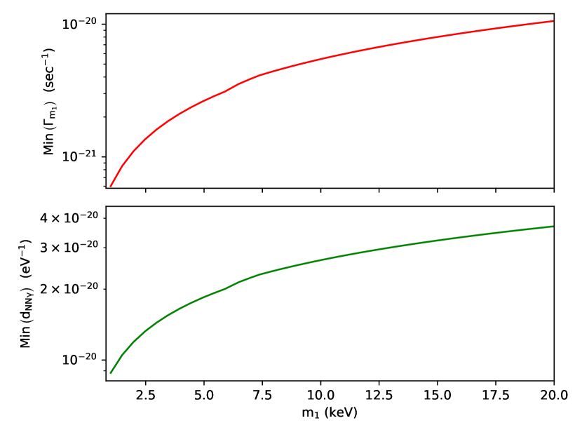
Figure 2: Top panel: The minimum required decay rate to explain the COB excess reported by LORRI for sterile neutrinos with masses ($1\leavevmode\nobreak\ \rm keV-20\leavevmode\nobreak\ \rm keV)$. Bottom panel: The corresponding minimum magnetic coupling strength $(d_{\rm NN\gamma})$ in $\text{eV}^{-1}$.

IV.2 Sterile to active neutrino decay

In this section, we consider the $\mathcal{O}$(eV) mass scale of sterile neutrino, which is decaying into active neutrino and photon via active-to-sterile transition magnetic dipole moment. This radiative decay process can be expressed as $N_{1}\to\nu_{a}+\gamma$. The wavelength of the emitted photon $(\lambda_{e})$ can be calculated from Eq. (4). The term $\lambda_{e}$ depends on both the mass of sterile and active neutrino. We then fix the active neutrino mass to $0.12\,\rm eV$. As explained earlier in section (IV.1), the required energy of the photons should be between $2\,\rm eV-10\,\rm eV$ such that these redshifting photons will be observed today as an excess radiation in the COB. Using these conditions, we find that the mass of the sterile neutrino will be in the range of $4\,\rm eV-20\,\rm eV$.

The upper bound on the mass of the sterile neutrino to be a dark matter candidate, derived from the Traemaine-Gunn bound, is $0.4$ keV Abazajian and Koushiappas (2006). Therefore, we examine the $\mathcal{O}$(eV) scale decaying sterile neutrinos, which may be considered as dark radiation. In the standard scenario case, only three neutrino species contribute to the $\rm N_{eff}^{SM}$ which is $3.044$. However, in a nonstandard scenario, the effective neutrino species can be written as $\rm N_{eff}=N_{eff}^{SM}+\Delta N_{eff}$, where $\Delta\rm N_{eff}$ comes from the additional relativistic components that take part in the dark radiation Abazajian and Koushiappas (2006). Dark radiation measures the amount of radiation energy contributed by the relativistic species except photons. Usually, neutrino oscillation anomalies give the idea for searching the new additional relativistic particles in the cosmos Abazajian and Koushiappas (2006). Motivated by the neutrino oscillation experiment for explaining the dark radiation, the mass range of sterile neutrino should be $m_{s}\lesssim\rm eV$ Drewes (2013). So here, we take the mass range $(4\,\rm eV-20\,\rm eV)$ of decaying sterile neutrino, which can be regarded as dark radiation.

The decay width for a decaying sterile neutrino via sterile-to-active transition magnetic moment is given by Beltrán et al. (2024)

$$\Gamma_{m_{1}}(m_{1}\rightarrow m_{2}+\gamma)=\frac{|d_{\rm\nu N\gamma}|^{2}}{2\pi}m_{1}^{3}\,,$$ (9)

where $d_{\nu\rm N\gamma}$, $m_{1}$, and $m_{2}$ represent the active-to-sterile transition magnetic dipole moment and the mass of the sterile and active neutrino, respectively. On the contrary to the decay width shown in Eq. (2), here $\Gamma_{m_{1}}$ is independent of the mass difference between the sterile and active neutrino. We then write the expression for the mean specific intensity $I_{\lambda}$ of photons produced from eV-scale decaying sterile neutrino as

$$I_{\lambda}=x\,\frac{c}{4\pi}\frac{{\Omega_{s}}{\rho_{c}}{c^{2}}\Gamma_{m_{1}}}{\lambda_{obs}(1+z)H(z)}.$$ (10)

Here, the term $x=1/2\,\left(1-m_{2}^{2}/m_{1}^{2}\right)$ is similar to the one shown in Eq. (4). Whereas, $\Omega_{s}$ represents the density parameter of sterile neutrinos, which can be expressed as $\Omega_{s}h^{2}=m_{1}/94.1\,\rm eV$ for a nonthermal scenario, which comes from the “Dodelson-Widrow Mechanism” Dodelson and Widrow (1994).

Using Eq. (10), we calculate $I_{\lambda}$ for $(4\,\rm eV-20\,\rm eV)$ mass range of sterile neutrinos, which can explain the flux of photons observed by LORRI in the wavelength range of $(0.4\,\rm\mu m-0.9\,\rm\mu m)$. For a fixed $\Gamma_{m_{1}}=1.04\times 10^{-22}\,\rm sec^{-1}$ and $m_{1}=7.56\,\rm eV$, we plot $I_{\lambda}$ versus the observed wavelength $\lambda_{obs}$ in Fig. 3. Then, in Fig. 3, we fix the total intensity of photons $I=8.06\pm 1.92\,\rm{nW/sr/\mu m}$ for a given mass of decaying sterile neutrino $m_{1}=7.56\,\rm eV$. The green-shaded region represents the specific intensity $I_{\lambda}$ for decaying dark matter detected observed by LORRI Bernal et al. (2021). Below, we calculate the decay rate for mass $m_{1}$ required to explain the COB excess anomaly.

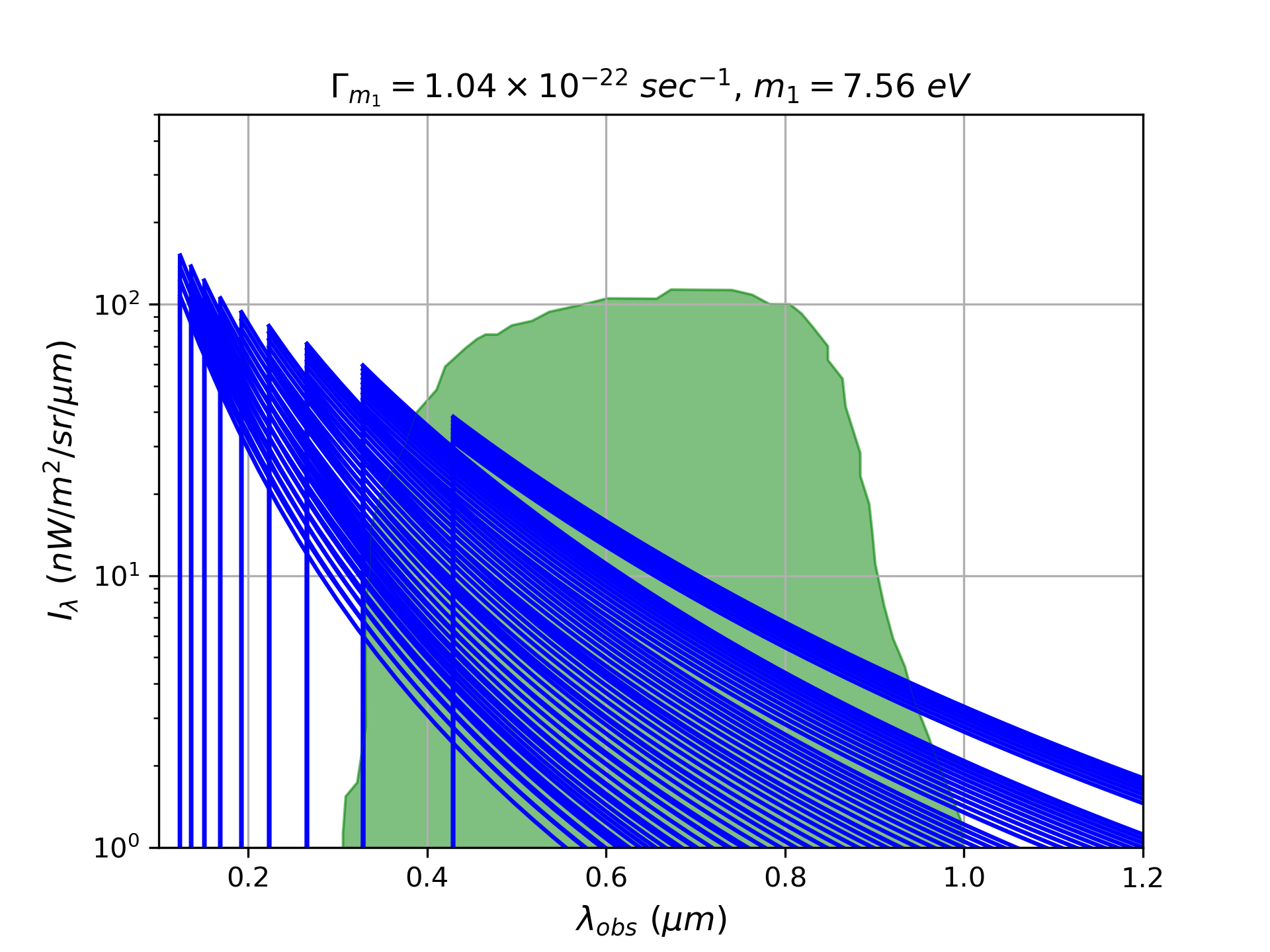
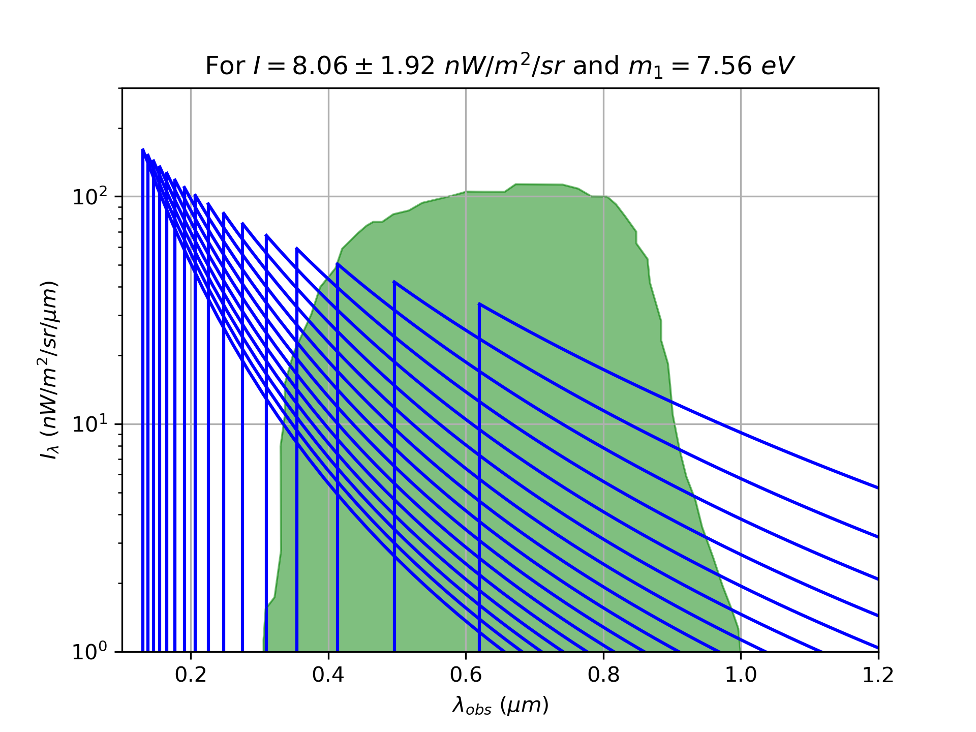
Figure 3: (a): represents the variation in specific intensity $I_{\lambda}$ with respect to $\lambda_{\rm obs}$, for given $\Gamma_{m_{1}}=1.04\times 10^{-22}\,\text{sec}^{-1}$ and $m_{1}=7.56\,\rm eV$. (b): The variations in $I_{\lambda}$ contributing to LORRI’s reported COB excess intensity, that is, the total intensity is equal to $8.06\pm 1.92\,\rm nW/m^{2}/sr$, for $\Gamma_{m_{1}}\sim(10^{-22}-10^{-21})\,\text{sec}^{-1}$ and $m_{1}=7.56\,\rm eV$. The green-shaded area illustrates the responsivity curve of LORRI for each detected wavelength, depicted with an unnormalized shape.

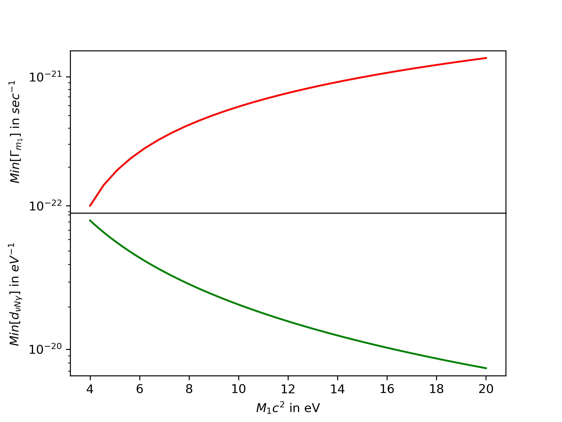
Figure 4: Top panel: The minimum required decay rate to explain the COB excess reported by LORRI for sterile neutrinos with masses ($4\leavevmode\nobreak\ \rm eV-20\leavevmode\nobreak\ \rm eV)$. Bottom panel: The corresponding minimum magnetic coupling strength $(d_{\rm\nu N\gamma})$ in $\text{eV}^{-1}$.

In Fig. 4, the red solid line shows the minimum decay width $\Gamma_{m_{1}}$ for sterile neutrino mass $(4\text{eV}\leq m_{1}\leq 20\text{eV})$ such that the total intensity $I=8.06\pm 1.92\,\rm{nW/sr/\mu m}$. We find that $\Gamma_{m_{1}}$ increases for heavier sterile neutrinos. This can be analysed from the fact that the specific intensity $(I_{\lambda})$ depends directly on the decay width while mass enters only through redshift $z(\lambda_{\rm obs},m_{1})$ which can only alter the Hubble parameter $H(z)$— as shown in Eq. (10). Thus, larger mass increases $z(\lambda_{\rm obs},m_{1})$, suggesting an early decay of sterile neutrino. However, as the intensity of photons redshifts more for an early decay which requires a larger decay width to obtain the required intensity today. Further, in the solid green line, we plot the minimum required active-to-sterile transition magnetic moment $d_{\nu N\gamma}$ derived for the red solid line using Eq. (9). We observe that $d_{\nu N\gamma}$ decreases with the increase of the mass of the decaying sterile neutrino. This can be analysed from Eq. (9), where $d_{\nu N\gamma}$ is inversely proportional to the mass of decaying sterile neutrinos. We find that, the required $d_{\nu N\gamma}$ to explain the anomaly lies between $\left(10^{-19}-10^{-20}\right)\,\rm eV^{-1}$ for sterile neutrino mass $4\,\rm eV\leq m_{1}\leq 20\,\rm eV$. In terms of the Bohr magneton, $d_{\nu N\gamma}$ take values of $3.33\times 10^{-13}\,\rm\mu_{B}-10^{-12}\,\rm\mu_{B}$.

Currently, the upper bound on the active-to-sterile transition dipole moment $d_{\rm\nu N\gamma}$ for sterile neutrino’s mass $4\,\rm eV\leq m_{1}\leq 20\,\rm eV$ remains unconstrained. There are several experimental upper bounds on the active-to-sterile transition magnetic dipole moment. Recent studies of XENON1T found that the upper bound on $d_{\nu N\gamma}\lesssim 6\times 10^{-11}\mu_{B}$ for several MeV mass range of sterile neutrino Shoemaker et al. (2021). However, the recent analysis of global clusters sets an upper limit as $d_{\nu N\gamma}\lesssim 1.2\times 10^{-12}\mu_{B}$ Cañas et al. (2016).

IV.3 Active-to-active neutrino magnetic moment

In the UV model, the active-to-active neutrino magnetic moment is naturally suppressed Beltrán et al. (2024). Active-sterile mixing can create an active-to-active neutrino magnetic moment in the broken phase parameters when the right-handed neutrinos are integrated out Beltrán et al. (2024). As such $d_{\nu\nu\gamma}\lesssim 2\times 10^{-8}\leavevmode\nobreak\ \text{\rm GeV}^{-1}$, we may anticipate that the active-to-active neutrino magnetic moments can satisfy the constraints from TEXONO Li et al. (2003), GEMMA Beda et al. (2010), LSND, and Borexino Agostini et al. (2017) in the inverse see-saw mechanism, where larger active-sterile mixing can occur. For the specified mass range $(0.12\leavevmode\nobreak\ \text{\rm eV}-0.7\leavevmode\nobreak\ \text{\rm eV})$ of active neutrinos, we are not able to obtain the specific intensity of photons due to the radiative decay of active neutrinos. As for this aforementioned mass range of active neutrinos, a very less number of photons can be generated, which cannot explain the COB excess anomaly in the observed wavelength range. For that reason, we cannot observe any specific intensity of photons in the observed wavelength range $\lambda_{obs}=0.2\leavevmode\nobreak\ \mu m-1.2\leavevmode\nobreak\ \mu m$ because to explain the COB excess anomaly, we need minimum $4$ eV mass of sterile neutrinos. To summarize, COB excess can be explained by the radiative decays of sterile neutrino through sterile-to-sterile and sterile-to-active transition magnetic dipole moment for ($1\,\rm keV-20\,\rm keV$) and ($4\,\rm eV-20\,\rm eV$) mass scale neutrinos, respectively.

V Conclusion and Outlook

Recent measurements of the cosmic optical background (COB) photon flux intensity by LORRI have revealed an excess beyond what is expected from deep galaxy counts. This excess may indicate a potential beyond the Standard Model (BSM) source of energetic photons. In this study, we considered the possibility of decaying sterile neutrinos producing photons and explored the corresponding decay rates. Notably, we did not account for photon energy generation through cascades involving other decay products. We found the required decay rate of sterile neutrino to explain the COB excess is of $\mathcal{O}(10^{-22}-10^{-20})\leavevmode\nobreak\ \text{sec}^{-1}$ for the keV mass range of the decaying sterile neutrino and for the $\mathcal{O}$(eV) mass range of the decaying sterile neutrino, the decay rate should be in the range of $\mathcal{O}(10^{-23}-10^{-22})\leavevmode\nobreak\ \text{sec}^{-1}$.

To explain the COB excess, we adopt a minimal framework involving sterile neutrinos within the effective field theory approach. The radiative decay of sterile neutrinos, resulting in photon production, is primarily governed by magnetic moments associated with sterile-to-sterile and sterile-to-active neutrino transitions. We calculate the sterile-to-sterile transition dipole moment strength $(d_{NN\gamma})$ and the sterile-to-active transition dipole moment strength ($d_{\nu N\gamma}$) for various mass-scales and decay rates. We find that, $d_{NN\gamma}$ take values of $3\times 10^{-14}\,\mu_{B}-10^{-13}\,\mu_{B}$ for sterile neutrinos of mass range $1\,\rm keV-20\,\rm keV$. Whereas sterile neutrinos, with mass range $4\,\rm eV-20\,\rm eV$, decaying via sterile-to-active transition magnetic moment $(d_{\nu\rm N\gamma})$ take values of $3.33\times 10^{-13}\,\mu_{B}-10^{-12}\,\mu_{B}$. Our minimal framework based on decaying sterile neutrinos of mass $\mathcal{O}$(keV) and $\mathcal{O}$(eV) successfully explains the COB excess.

VI Acknowledgement

We sincerely acknowledge the usage of python packages scipy and astropy. We thank Rahul Kothari for his earlier collaboration on this project.

References

- Kovetz et al. (2017) E. D. Kovetz et al., (2017), arXiv:1709.09066 [astro-ph.CO] .
- Kovetz et al. (2020) E. D. Kovetz et al., Bull. Am. Astron. Soc. 51, 101 (2020), arXiv:1903.04496 [astro-ph.CO] .
- Grin et al. (2007) D. Grin, G. Covone, J.-P. Kneib, M. Kamionkowski, A. Blain, and E. Jullo, Phys. Rev. D 75, 105018 (2007), arXiv:astro-ph/0611502 .
- Gong et al. (2016) Y. Gong, A. Cooray, K. Mitchell-Wynne, X. Chen, M. Zemcov, and J. Smidt, Astrophys. J. 825, 104 (2016), arXiv:1511.01577 [astro-ph.CO] .
- Creque-Sarbinowski and Kamionkowski (2018) C. Creque-Sarbinowski and M. Kamionkowski, Phys. Rev. D 98, 063524 (2018), arXiv:1806.11119 [astro-ph.CO] .
- Bernal et al. (2022) J. L. Bernal, G. Sato-Polito, and M. Kamionkowski, Physical Review Letters 129, 231301 (2022).
- Zemcov et al. (2017a) M. Zemcov, P. Immel, C. Nguyen, A. Cooray, C. M. Lisse, and A. R. Poppe, Nature Communications 8, 15003 (2017a).
- Zemcov et al. (2017b) M. Zemcov, P. Immel, C. Nguyen, A. Cooray, C. M. Lisse, and A. R. Poppe, Nature Commun. 8, 5003 (2017b), arXiv:1704.02989 [astro-ph.IM] .
- Lauer et al. (2021a) T. R. Lauer et al., Astrophys. J. 906, 77 (2021a), arXiv:2011.03052 [astro-ph.GA] .
- Lauer et al. (2021b) T. R. Lauer, M. Postman, H. A. Weaver, J. R. Spencer, S. A. Stern, M. W. Buie, D. D. Durda, C. M. Lisse, A. Poppe, R. P. Binzel, et al., The Astrophysical Journal 906, 77 (2021b).
- Conselice et al. (2016) C. J. Conselice, A. Wilkinson, K. Duncan, and A. Mortlock, The Astrophysical Journal 830, 83 (2016).
- Yue et al. (2013) B. Yue, A. Ferrara, R. Salvaterra, Y. Xu, and X. Chen, Monthly Notices of the Royal Astronomical Society 433, 1556 (2013).
- Cooray (2016) A. Cooray, Royal Society Open Science 3, 150555 (2016).
- Matsumoto and Tsumura (2019) T. Matsumoto and K. Tsumura, Publications of the Astronomical Society of Japan 71, 88 (2019).
- Nakayama and Yin (2022) K. Nakayama and W. Yin, Phys. Rev. D 106, 103505 (2022), arXiv:2205.01079 [hep-ph] .
- Carenza et al. (2023) P. Carenza, G. Lucente, and E. Vitagliano, Phys. Rev. D 107, 083032 (2023), arXiv:2301.06560 [hep-ph] .
- Ge and Pasquini (2023a) S.-F. Ge and P. Pasquini, Journal of High Energy Physics 2023, 1 (2023a).
- Ge and Pasquini (2023b) S.-F. Ge and P. Pasquini, Physics Letters B 841, 137911 (2023b).
- Voloshin (1987) M. Voloshin, On compatibility of small mass with large magnetic moment of neutrino, Tech. Rep. (Gosudarstvennyj Komitet po Ispol’zovaniyu Atomnoj Ehnergii SSSR, 1987).
- Barbieri and Mohapatra (1989) R. Barbieri and R. N. Mohapatra, Physics Letters B 218, 225 (1989).
- Babu et al. (2020) K. Babu, S. Jana, and M. Lindner, Journal of High Energy Physics 2020, 1 (2020).
- Babu et al. (2021) K. Babu, S. Jana, M. Lindner, and V. PK, Journal of High Energy Physics 2021, 1 (2021).
- Schwetz et al. (2021) T. Schwetz, A. Zhou, and J.-Y. Zhu, Journal of High Energy Physics 2021, 1 (2021).
- Barducci et al. (2023) D. Barducci, E. Bertuzzo, M. Taoso, and C. Toni, Journal of High Energy Physics 2023, 1 (2023).
- Günther et al. (2024) J. Y. Günther, J. de Vries, H. K. Dreiner, Z. S. Wang, and G. Zhou, Journal of High Energy Physics 2024, 1 (2024).
- Beltrán et al. (2024) R. Beltrán, P. D. Bolton, F. F. Deppisch, C. Hati, and M. Hirsch, arXiv preprint arXiv:2405.08877 (2024).
- Aguilar-Arevalo et al. (2021) A. A. Aguilar-Arevalo, B. C. Brown, J. M. Conrad, R. Dharmapalan, A. Diaz, Z. Djurcic, D. A. Finley, R. Ford, G. T. Garvey, S. Gollapinni, A. Hourlier, E.-C. Huang, N. W. Kamp, G. Karagiorgi, T. Katori, T. Kobilarcik, K. Lin, W. C. Louis, C. Mariani, W. Marsh, G. B. Mills, J. Mirabal-Martinez, C. D. Moore, R. H. Nelson, J. Nowak, I. Parmaksiz, Z. Pavlovic, H. Ray, B. P. Roe, A. D. Russell, A. Schneider, M. H. Shaevitz, H. Siegel, J. Spitz, I. Stancu, R. Tayloe, R. T. Thornton, M. Tzanov, R. G. Van de Water, D. H. White, and E. D. Zimmerman (MiniBooNE Collaboration), Phys. Rev. D 103, 052002 (2021).
- Aguilar-Arevalo et al. (2018) A. A. Aguilar-Arevalo, B. C. Brown, L. Bugel, G. Cheng, J. M. Conrad, R. L. Cooper, R. Dharmapalan, A. Diaz, Z. Djurcic, D. A. Finley, R. Ford, F. G. Garcia, G. T. Garvey, J. Grange, E.-C. Huang, W. Huelsnitz, C. Ignarra, R. A. Johnson, G. Karagiorgi, T. Katori, T. Kobilarcik, W. C. Louis, C. Mariani, W. Marsh, G. B. Mills, J. Mirabal, J. Monroe, C. D. Moore, J. Mousseau, P. Nienaber, J. Nowak, B. Osmanov, Z. Pavlovic, D. Perevalov, H. Ray, B. P. Roe, A. D. Russell, M. H. Shaevitz, J. Spitz, I. Stancu, R. Tayloe, R. T. Thornton, M. Tzanov, R. G. Van de Water, D. H. White, D. A. Wickremasinghe, and E. D. Zimmerman (MiniBooNE Collaboration), Phys. Rev. Lett. 121, 221801 (2018).
- Aguilar et al. (2001) A. Aguilar, L. B. Auerbach, R. L. Burman, D. O. Caldwell, E. D. Church, A. K. Cochran, J. B. Donahue, A. Fazely, G. T. Garvey, R. M. Gunasingha, R. Imlay, W. C. Louis, R. Majkic, A. Malik, W. Metcalf, G. B. Mills, V. Sandberg, D. Smith, I. Stancu, M. Sung, R. Tayloe, G. J. VanDalen, W. Vernon, N. Wadia, D. H. White, and S. Yellin (LSND Collaboration), Phys. Rev. D 64, 112007 (2001).
- Atre et al. (2009) A. Atre, T. Han, S. Pascoli, and B. Zhang, Journal of High Energy Physics 2009, 030 (2009).
- Bondarenko et al. (2018) K. Bondarenko, A. Boyarsky, D. Gorbunov, and O. Ruchayskiy, Journal of High Energy Physics 2018 (2018).
- Balantekin and Vassh (2014) A. Balantekin and N. Vassh, Physical Review D 89, 073013 (2014).
- Gninenko and Krasnikov (1999) S. Gninenko and N. Krasnikov, Physics Letters B 450, 165 (1999).
- Derbin et al. (1993) A. Derbin, A. Chernyǐ, L. Popeko, V. Muratova, G. Shishkina, and S. Bakhlanov, Soviet Journal of Experimental and Theoretical Physics Letters 57, 768 (1993).
- Liu et al. (2004) D. Liu, Y. Ashie, S. Fukuda, Y. Fukuda, K. Ishihara, Y. Itow, Y. Koshio, A. Minamino, M. Miura, S. Moriyama, et al., Physical review letters 93, 021802 (2004).
- Agostini et al. (2017) M. Agostini, K. Altenmüller, S. Appel, V. Atroshchenko, Z. Bagdasarian, D. Basilico, G. Bellini, J. Benziger, D. Bick, G. Bonfini, et al., Physical Review D 96, 091103 (2017).
- Arpesella et al. (2008) C. Arpesella, H. Back, M. Balata, G. Bellini, J. Benziger, S. Bonetti, A. Brigatti, B. Caccianiga, L. Cadonati, F. Calaprice, et al., Physical Review Letters 101, 091302 (2008).
- Carenza et al. (2024) P. Carenza, G. Lucente, M. Gerbino, M. Giannotti, and M. Lattanzi, Physical Review D 110, 023510 (2024).
- Capozzi and Raffelt (2020) F. Capozzi and G. Raffelt, Physical Review D 102, 083007 (2020).
- Alexander (2016) S. Alexander, in Journal of Physics: Conference Series, Vol. 718 (IOP Publishing, 2016) p. 062076.
- Chen and Kamionkowski (2004) X.-L. Chen and M. Kamionkowski, Phys. Rev. D 70, 043502 (2004), arXiv:astro-ph/0310473 .
- Bernal et al. (2021) J. L. Bernal, A. Caputo, and M. Kamionkowski, Phys. Rev. D 103, 063523 (2021), [Erratum: Phys.Rev.D 105, 089901 (2022)], arXiv:2012.00771 [astro-ph.CO] .
- Abazajian and Koushiappas (2006) K. Abazajian and S. M. Koushiappas, Physical Review D—Particles, Fields, Gravitation, and Cosmology 74, 023527 (2006).
- Madau (1995) P. Madau, Astrophys. J. 441, 18 (1995).
- Inoue et al. (2014) A. K. Inoue, I. Shimizu, and I. Iwata, Mon. Not. Roy. Astron. Soc. 442, 1805 (2014), arXiv:1402.0677 [astro-ph.CO] .
- Drewes (2013) M. Drewes, International Journal of Modern Physics E 22, 1330019 (2013).
- Dodelson and Widrow (1994) S. Dodelson and L. M. Widrow, Physical Review Letters 72, 17 (1994).
- Shoemaker et al. (2021) I. M. Shoemaker, Y.-D. Tsai, and J. Wyenberg, Physical Review D 104, 115026 (2021).
- Cañas et al. (2016) B. C. Cañas, O. Miranda, A. Parada, M. Tortola, and J. W. Valle, Physics Letters B 753, 191 (2016).
- Li et al. (2003) H. Li, J. Li, H. Wong, C. Chang, C. Chen, J. Fang, C. Hu, W. Kuo, W. Lai, F. Lee, et al., Physical review letters 90, 131802 (2003).
- Beda et al. (2010) A. Beda, V. Brudanin, V. Egorov, D. Medvedev, M. Shirchenko, and A. Starostin, Physics of Particles and Nuclei Letters 7, 406 (2010).