moo
\IfValueF#2
A:
#1
\IfValueT#2\IfValueF#3
A:
#1
\IfValueT#3
\marginnote
A:
#1
\NewDocumentCommand\delm
#1
\NewDocumentCommand\addm#1
\coltauthor
\NameAnastasis Kratsios \Emailkratsioa@mcmaster.ca
\addrThe Vector Institute and McMaster University
and \NameTakashi Furuya
\Emailtakashi.furuya0101@gmail.com
\addrShimane University
Is In-Context Universality Enough?
MLPs are Also Universal In-Context
Abstract
The success of transformers is often linked to their ability to perform in-context learning. Recent work shows that transformers are universal in context, capable of approximating any real-valued continuous function of a context (a probability measure over ) and a query . This raises the question: Does in-context universality explain their advantage over classical models? We answer this in the negative by proving that MLPs with trainable activation functions are also universal in-context. This suggests the transformer’s success is likely due to other factors like inductive bias or training stability.
1 Introduction
The undeniable success of transformers is attributed to their ability to learn in-context, unlike traditional multilayer perceptions (MLPs). This means that transformers can process sequences of tokens and predict the next relevant token. They often exhibit in-context learning (ICL) when trained on large, diverse datasets. This means that given a short sequence of input-output pairs (a prompt) from a specific task, the model can make predictions on new examples without updating its parameters.
There are three primary pillars in which ICL can be studied: approximation theoretic, statistical, and optimization lenses. We focus on the former of these lenses by contrasting the approximation capacity of the transformer with the classical MLP model by asking
| “Does the transformer have an approximation-theoretic advantage over the MLP?” | (Q) |
Due to the work of [Hornik et al.(1989)Hornik, Stinchcombe, and White, Yarotsky(2018), Suzuki(2018), Bolcskei et al.(2019)Bolcskei, Grohs, Kutyniok, and Petersen, Kidger and Lyons(2020), Kratsios and Papon(2022), Shen et al.(2022)Shen, Yang, and Zhang], and several others, it is by now well-known that MLPs are universal approximators in the classical “out-of-context” sense; i.e., meaning that any continuous functions from to can be uniformly approximated on compact sets to arbitrary precision by MLPs with enough neurons. These classical “out-of-context” universal approximation guarantees have since been established for the transformer model [Kim et al.(2024)Kim, Nakamaki, and Suzuki, Fang et al.(2022)Fang, Ouyang, Zhou, and Cheng] with matching optimal rates, implying that the transformer is at least as expressive as the MLP “out-of-context”.
More recently [Petrov et al.(2025)Petrov, Lamb, Paren, Torr, and Bibi] showed that recurrent transformers can approximate any function in-context by leveraging prompt engineering. It was subsequently established by [Furuya et al.(2024)Furuya, de Hoop, and Peyré] that transformers are universal approximators in-context, meaning that they can approximate any function which continuously maps context and queries to predictions uniformly on compact sets to arbitrary precision; again given enough neurons. These results suggest that the transformer may indeed have an advantage in expressivity over the vintage MLP model, hinting that (Q) can be hoped to be answered positively since the latter is currently not known to be universal in-context.
Our paper is in the negative direction of (Q). Our main result (Theorem 3.1) matches the in-context universality of the MLP model in the setting of permutation invariant contexts (PICs) of [Castin et al.(2024)Castin, Ablin, and Peyré, Furuya et al.(2024)Furuya, de Hoop, and Peyré]. We conclude that if the transformer’s superior empirical performance over the MLP model cannot be explained by in-context universality. This suggests that the empirically well-documented advantage of transformers over MLPs must stem from a statistical or optimization phenomenon unique to transformers rather than from in-context universality.
Our main result is complemented by Corollary 3.2, which a quantitative version of [Furuya et al.(2024)Furuya, de Hoop, and Peyré], showing that for any target function, compact set of PICs, and approximation error, a transformer with multiple attention heads per block. Thus, the in-context approximation power of the transformer seems to match that of the MLP.
1.1 Secondary Contributions
Our second main result (Corollary 3.2) is deduced from our main result for ReLU MLPs, using our transformerification procedure (Proposition 4.6), which converts any MLP to a multi-head transformer which exactly preserves its depth and width while only doubling its trainable (non-zero) parameters (thus has the same order of trainable parameters) and with a fixed number of attention heads per block. This type of “conversion” map was also recently obtained to prove quantitative universal approximation guarantees for convolutional neural networks in [Petersen and Voigtlaender(2020)] and spiking neural networks in [Singh et al.(2023)Singh, Fono, and Kutyniok].
A key step in our analysis shows that ReLU MLPs can exactly implement the -Wasserstein distance on a broad class of finite probability measures, containing all empirical measures (Proposition D.14). This auxiliary result can be of independent interest to the neural optimal transport community, e.g. [Korotin et al.(2019)Korotin, Egiazarian, Asadulaev, Safin, and Burnaev, Korotin et al.(2022)Korotin, Selikhanovych, and Burnaev, Gazdieva et al.(2024)Gazdieva, Choi, Kolesov, Choi, Mokrov, and Korotin].
1.2 Related Literature
Permutation-Invariant Contexts and their Geometry
Transformer models generally cannot inherently detect the order of input tokens without using positional encodings [Vaswani et al.(2017)Vaswani, Shazeer, Parmar, Uszkoreit, Jones, Gomez, Kaiser, and Polosukhin, Chu et al.(2022)Chu, Tian, Zhang, Wang, and Shen, Li et al.(2021)Li, Si, Li, Hsieh, and Bengio]. These encodings capture the sequence in which tokens appear, addressing the transformer’s invariance to row permutations in the input context matrix. Since we are studying the transformer architecture and not a specific positional encoding scheme; then, we will adopt the permutation-invariant formulation of context of [Castin et al.(2024)Castin, Ablin, and Peyré, Furuya et al.(2024)Furuya, de Hoop, and Peyré], rather than the sequential formulation of [Garg et al.(2022)Garg, Tsipras, Liang, and Valiant, Zhang et al.(2024a)Zhang, Frei, and Bartlett, Akyürek et al.(2022)Akyürek, Schuurmans, Andreas, Ma, and Zhou, Von Oswald et al.(2023)Von Oswald, Niklasson, Randazzo, Sacramento, Mordvintsev, Zhmoginov, and Vladymyrov], which does not capture the transformer’s permutation invariance.
In this paper, we work with a refined version of the permutation-invariant setting introduced by [Furuya et al.(2024)Furuya, de Hoop, and Peyré]. Their framework formalizes contexts as probability measures on a space of tokens within a dictionary . The motivation is that any finite set of tokens can be represented as an empirical measure , where (summing to ), reflecting the relative frequency of each token in the permutation-invariant context (PIC) , which is unaffected by the indexing of these tokens. While their permutation-invariant setting is well-suited for real-world transformers, it overlooks the fact that real-world context windows (), even when tokens are drawn from an infinite dictionary , still impose constraints.
Our analysis rests on a quantitative refinement of the mathematical idealization in the setting of [Furuya et al.(2024)Furuya, de Hoop, and Peyré], which assumed that context can be arbitrarily large since any real-world LLM has a finite context window. Instead, our analysis operates on the realistic subspace (formalized in Section 2.1) comprised of probability measures of the form where the weights are all positive and divisible by the context window . Thus, each distinctly observed token cannot be observed more times than the context window allows. I.e. we prohibit mathematical artifacts such as a relative frequency of . Under this realism restriction, we can identify any PIC in an equivalence class of real-matrix
| (1) |
here, denotes the equivalence class of matrices formed by permuting the rows of the matrix . We equip with the -Wasserstein metric, which, when restricted to the space of empirical measures , is shown to be equivalent to the natural quotient metric (see [Bridson and Haefliger(1999)]) on the corresponding subspace of matrices, quotiented by row permutations. Details are provided in Section 2.1.
Approximation Guarantees
We highlight that there are alternative, weaker, approximation guarantees for transformers than the one in [Furuya et al.(2023)Furuya, Puthawala, Lassas, and de Hoop], some of which consider contexts; e.g. [Petrov et al.(2025)Petrov, Lamb, Paren, Torr, and Bibi], without permutation-invariance, and some which are context-free; e.g. [Kim et al.(2024)Kim, Nakamaki, and Suzuki, Fang et al.(2022)Fang, Ouyang, Zhou, and Cheng]. The conclusion remains the same when juxtaposed against Theorem 3.1; in-context universality is not enough to explain the advantage of the transformer model over the classical MLP model.
Although not directly related to our findings, there is a body of work that examines the expressivity of transformers when applied to discrete token sets as formal systems [Chiang et al.(2023)Chiang, Cholak, and Pillay, Merrill and Sabharwal(2023), Strobl et al.(2024)Strobl, Merrill, Weiss, Chiang, and Angluin, Olsson et al.(2022)Olsson, Elhage, Nanda, Joseph, DasSarma, Henighan, Mann, Askell, Bai, Chen, et al.]. Another line of research also explores how positional encoding affects transformer expressivity [Luo et al.(2022)Luo, Li, Zheng, Liu, Wang, and He]. Nevertheless, the transformer’s advantage over the classical MLP model is not identified. We also mention results explaining the ability of transformers to represent specific structures, such as Kalman filtering updates relying on a Nadaraya–Watson kernel density estimator [Goel and Bartlett(2024)] and its ability to satisfy certain constraints [Kratsios et al.(2021)Kratsios, Zamanlooy, Liu, and Dokmanić].
Statistical Guarantees
We also mention the growing body of statistical guarantees for in-context learners, such as transformers. These study the training dynamics of transformers with linear attention mechanisms [Chen et al.(2024)Chen, Sheen, Wang, and Yang, Lu et al.(2024)Lu, Letey, Zavatone-Veth, Maiti, and Pehlevan, Zhang et al.(2024b)Zhang, Wu, and Bartlett, Siyu et al.(2024)Siyu, Heejune, Tianhao, and Zhuoran, Kim and Suzuki(2024b)] and non-asymptotic single-step variants thereof [Duraisamy(2024)], the minimax statistical optimality of pre-trained transformers trained in-context [Kim et al.(2024)Kim, Nakamaki, and Suzuki], guarantees for transformers trained with non-i.i.d. time-series data [Limmer et al.(2024)Limmer, Kratsios, Yang, Saqur, and Horvath], PAC-Bayesian guarantees for transformers [Mitarchuk et al.(2024)Mitarchuk, Lacroce, Eyraud, Emonet, Habrard, and Rabusseau], their infinite-width limits [Zhang et al.(2024a)Zhang, Frei, and Bartlett] in an NTK fashion [Jacot et al.(2018)Jacot, Gabriel, and Hongler], statistical guarantees for in-context classification using transformers [Reddy(2023)], and several other works examining the statistical foundations of in-context learning; e.g. [Akyürek et al.(2022)Akyürek, Schuurmans, Andreas, Ma, and Zhou, Li et al.(2023)Li, Ildiz, Papailiopoulos, and Oymak, Bai et al.(2024)Bai, Chen, Wang, Xiong, and Mei]. We mention the recent line of work studying the efficiency of trains of thoughts generated by transformers trained in context [Kim and Suzuki(2024a)].
2 Preliminaries
This section contains the necessary background for the formulation of our main results.
2.1 Permutation-Invariant In-Context Learners
We first review and add to the notions of permutation invariant in context-learners considered in [Furuya et al.(2024)Furuya, de Hoop, and Peyré]. This relies on the introduction of some tools from probability theory, specifically from optimal transport and their refinements use ideas from metric geometry; both of which are introduced now.
Permutation-Invariant Context via Probability Measures
Given a (non-empty) measurable subset of , for some , we use to denote the set of all Borel probability measures on which is then equipped with the topology of weak convergence of measures. When , we denote by the subset of probabilities that finitely integrate for some (and thus for any) . Similarly, we equip with the Wasserstein -distance , that is, for , the metric defined by where . Elements of are called couplings, or transport plans, between the measures and . When the Kantorovich-Rubinstein duality allows us to re-express and extend the definition of to the class of finite signed (Borel) measures on via
where denotes the set of -Lipschitz functions on with , where is the optimal Lipschitz constant of and . This extension to signed finite measures is typical in the non-linear theory of Banach space theory [Godefroy(2015), Weaver(2018), Ambrosio and Puglisi(2020)] and has applications in deep learning [von Luxburg and Bousquet(2004), Kratsios et al.(2023)Kratsios, Liu, Lassas, de Hoop, and Dokmanić, Cuchiero et al.(2023)Cuchiero, Schmocker, and Teichmann].
Though infinite-length contexts are considered in some parts of the literature, contexts of a finite but possibly very large are both more representative of practical use-cases of ICL. They are more amenable to precise quantitative analysis. Thus, in this paper, we fix: a finite context window , a token number of contextual data, and a dictionary set with at-least distinct points. We define the contextualized simplex
| (2) |
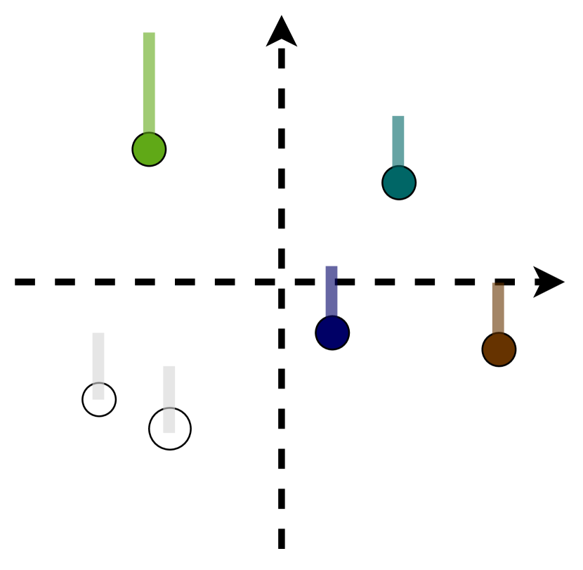
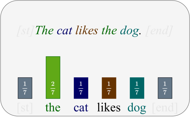
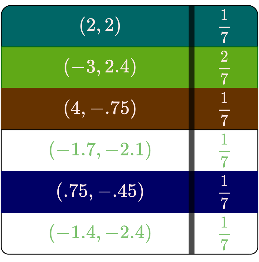
In this illustration, there are tokens: “the”, “cat”, “likes”, “dog”, as well as the punctuation tokens indicating the start “[st]”, and end “[end]” of the sentence in the illustrated prompt. Only “the” is repeated twice, and the context window .
In short, is a discretization of the relative interior of the -simplex. The space PICs consists of all probability measures in counting mass on at-most distinct tokens where each token appears at-most times; formalized as follows.
Definition 2.1 (Permutation-Invariant Context).
Let and be non-empty. The space of permutation-invariant contexts (PICs) on is the metric subspace of consisting of all satisfying
| (3) |
Probability measures provide an intuitive mechanism by which we may interpret the frequency of any context in a given context window while ignoring ad-hoc orders due to the permutation invariance of the points representing any . Nevertheless, most deep learning models such as transformers, GNNs, or MLPs do not act on measures but on matrices. To bridge the link between our mathematically natural formulation of PIC in (3) and the input/outputs of these models, we first identify PICs with certain equivalence classes of matrices.
Matrix Representations of PICs
Let denote the set of matrices whose rows are given by and such that .
We quotient by the equivalence relation if there is a permutation matrix for which . Our analysis relies on the map
| (4) |
which is easily verified to be a bijection between and . The identification in (4) allows us to put a metric structure on which is identical to the -Wasserstein distance on inherited from . This metric, which simply denote by , sends any pair of and of equivalence classes of matrices in to
| (5) |
Thus, by construction metrized by is isometric (i.e. indistinguishable as a metric space) from equipped with the -Wasserstein distance on signed finite measures, as defined in [Villani(2009)] on probability measures on [Ambrosio and Puglisi(2020)] on finite measures.
A Geometric Interpretation of the Metric
Before moving on, we further motivate the choice of metric by considering the special case where the context window exactly equals to the number of tokens . In this case, each weight in (3) and consists only of empirical measures with distinct support points in . Whence, is identifiable with the space of equivalence classes of matrices with distinct rows, up to row permutation and the identification in (4) simplifies to
| (6) |
Now, is the quotient space of the space , namely, the space of matrices with distinct rows, by (row) permutations. We, momentarily, equip with the Fröbenius norm . Since the space of permutation matrices is a finite group acting by isometries on ; i.e. for each and every we have
then [Bridson and Haefliger(1999), Exercise 8.4 (3) - page 132] guarantees that the (natural) quotient topology on is metrized by the metric defined for any in by . The geometric motivation for is drawn from the fact that on .
Proposition 2.2 (Equivalence of and the Natural Quotient Metric on PICs).
Let and let be non-empty. Then, there are absolute constant such that: for each we have
In particular, the map is a homomorphism.
Furthermore, metrizes the natural quotient topology on .
Proposition 2.2 shows that is well-motivated in that it is equivalent to the most natural metric structure on the quotient space , at-least, in the special case where .
2.1.1 The Size of Sets of PICs
This section quantifies the size of compact sets of PICs. The reader not interested in quantitative universal approximation guarantees is encouraged to skip it.
Basic Definitions
Fix a compact set of contexts in . We denote the ball at any point of radius by . We say that are -separated, for some , if .
Metric Notions of Dimension
We say is -doubling if there is a constant such that: for each pair of radii and every subset of diameter at-most , there is no more than point in which are -separated. The minimum (infimum) such number is called the doubling (Assouad) dimension of .
Every such compact doubling metric space carries a (Borel) measure which ascribes such that, there is a “doubling constant” with the property that: for each and each we have , see [Cutler(1995), Theorem 3.16] and [Luukkainen and Saksman(1998)]. Examples include the uniform measure on and the normalized Riemannian measure on a compact Riemannian manifold. Unlike these familiar measures, which are compatible with their metric structure, some general metric spaces admit pathological metric measures which are incompatible with their metric dimension; see [Järvenpää et al.(2010)Järvenpää, Järvenpää, Käenmäki, Rajala, Rogovin, and Suomala, Example 3.1]. To avoid these pathologies, we focus on Ahlfors -regular measures on which attribute mass to any ball of radius in ; i.e. there are constants such that: for and every
| (7) |
We summarize the doubling and Ahlfors regularity requirements as follows.
Definition 2.3 (-Dimensional PIC).
Let . A compact subset of PICs equipped with a Borel probability measure is said to be -dimensional, its doubling dimension is and is Ahlfors -regular.
The compatibility between the metric structure on and the measure given by the Ahlfors condition in condition (7) allows us to intrinsically quantify the size of subsets of on which our approximation may fail. These subsets, illustrated later as the small trifling region in Figure 6, are non-Euclidean versions of the trifling regions in classical optimal universal approximation guarantees for MLPs; as in [Shen et al.(2022)Shen, Yang, and Zhang].
2.2 Deep Learning and Transformers
![[Uncaptioned image]](/html/2502.03327/assets/Bookkeeping/Images/SuperKhan.png)
| (8) |
Trainable Activation Functions
As most modern deep learning implementations, such as transformers using trainable Swish [Ramachandran et al.(2017)Ramachandran, Zoph, and Le] or GLU activation variants [Shazeer(2020)], KANs [Liu et al.(2024)Liu, Wang, Vaidya, Ruehle, Halverson, Soljačić, Hou, and Tegmark, Ismailov(2024)] activated by trainable B-splines and SiLUs, or neural snowflakes which implement trainable fractal activation functions [de Ocáriz Borde and Kratsios(2023), Borde et al.(2024a)Borde, Kratsios, Law, Dong, and Bronstein], have shifted towards trainable activation functions. We follow suit by using trainable activation functions in our MLPs, which can implement the Swish and leaky ReLUs activation function, skip connections blocks, and , see Appendix A for details and defined by
The MLP Model
In what follows, we will often make use of fully-connected MLPs with activation function as in (8). For any , we recall that an MLP with activation function is a map with iterative representation
| (9) |
where runs from to and for each is a matrix with and . Here, is the depth of the transformer and is its width.
Transformers with Multi-Head Attention
Building on the notation in (9), we formalize a transformer model. We thus first formalize a single attention head of [Bahdanau et al.(2014)Bahdanau, Cho, and Bengio], with temperature parameter , as a map sending any PIC to the following probability measure in
A transformer network operates by iteratively applying deep ReLU MLPs to the rows of its input matrix and then applying the attention mechanisms matrix-wise. Thus, a transformer with multi-head attention is a map sending any to , where is defined recursively by
| (10) |
where , runs from to and, for each , is a bias matrix, , and . Here, is called the depth of the transformer, is the maximum number of attention heads, and is called its width.
Our transformers mirror approximation guarantees for the MLP model, which do not include regularization layers such as skip connections or normalization. We are using the standard multi-head attention mechanism and we do not considered in the PIC guarantees of [Furuya et al.(2024)Furuya, de Hoop, and Peyré], [Petrov et al.(2025)Petrov, Lamb, Paren, Torr, and Bibi], nor a single linearized surrogate head attention of real-world multi-head attention mechanisms, as is often studied in the statistical literature [Zhang et al.(2024a)Zhang, Frei, and Bartlett, Lu et al.(2024)Lu, Letey, Zavatone-Veth, Maiti, and Pehlevan, Kim et al.(2024)Kim, Nakamaki, and Suzuki], or a single attention head as in [Kratsios et al.(2023)Kratsios, Liu, Lassas, de Hoop, and Dokmanić, Kim et al.(2024)Kim, Nakamaki, and Suzuki].
3 Main Result
Setting 1
Fix context lengths , dimensions , and subsets and with closed. Let be a modulus of continuity and be a compact subset of PICs. Let be an Ahlfors -regular probability measure on .
Theorem 3.1 (MLPs are Universal Approximators for PICs).
In the Setting 1, for any uniformly continuous with an increasing modulus of continuity . For each -uniformly continuous contextual mapping and approximation error and every confidence level : there is a ReLU MLP satisfying:
-
(i)
High-Probability Uniform Estimate: We have the typical uniform estimate
-
(ii)
Tail-Estimates: On the “bad” set : we have the tail-estimate
If is -dimensional and is large enough then, the depth and width of are and , respectively.
Setting and taking , then we see that every probability measure in is of the form for some . Thus, is in bijection (actually homeomorphic) with . Thus, Theorem 3.1 implies the simple formulation in (3.1) which is a quantitative version of that considered in [Furuya et al.(2024)Furuya, de Hoop, and Peyré] but for the classical ReLU MLP model in place of the transformer network with single attention-head per block.
We conclude our analysis by showing that our main result for MLPs directly implies the same conclusion for transformers with multiple attention heads per transformer block. Thus, we obtain a quantitative version of the main theorem in [Furuya et al.(2024)Furuya, de Hoop, and Peyré] as a direct consequence of our main result. The following key result allows us to represent MLPs as transformers with sparse MLPs.
Corollary 3.2 (Multihead Transformers version of Theorem 3.1).
In the setting of Theorem 3.1 and suppose that is -dimensional. For large enough, there is a transformer , taking values in , and satisfying:
Moreover, the depth and width of are and , respectively, and has exactly attention heads per transformer block.
4 Unpacking The Construction
We now explain our main result, namely Theorem 3.1.
4.1 Step 1 - Regular Decomposition of The (PI) Context Space
Fix a compact set . Figure 6 showcases the near piecewise constant partition of unity, which we will use to construct our approximating MLPs and multi-head transformers. The idea is to subdivide into a parts, and to construct MLPs which implement piecewise constant function with a value on each piece. This construction is a non-Euclidean version of the trifling regions approach for classical ReLU MLP approximation of functions on the cube considered in [Shen et al.(2022)Shen, Yang, and Zhang]; there, the authors decomposed in disjoint (up to their boundary) sub-cubes which can be understood as Balls with respect to the metric on . That classical case was simple since balls (sub-cubes) can be chosen to be disjoint (up to their boundaries), meaning that the Voronoi cells are (up to their boundary) equal to balls; e.g.
In contrast, in general, metric spaces such as one cannot ensure that metric balls are disjoint. Unlike sub-cubes of which align perfectly, these metric balls need not do so in . Thus, we need to manually create disjoint regions by iteratively deleting overlapping regions between balls. The result, illustrated in Figure 6 is constructed as follows.
Let , and -packing of , and ; for each recursively define the retracted Voronoi cells by
| (11) |
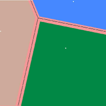
Our approximators will uniformly approximate the given target PIC-function on the approximation region covered by the retracted Voronoi cells . Our approximator will be continuous and piecewise constant, one (possibly distinct) value on each retracted Voronoi cell , and that value is given by the target PIC-function’s value at that cell’s landmark point . The approximation region and trifling region are
| (12) |
We can ensure that the trifling region is small. For class -type approximation guarantees, with , the “smallness” of the trifling region in [Shen et al.(2022)Shen, Yang, and Zhang] guaranteed by it having a small Lebesgue measure. Here, in our non-Euclidean setting, the smallness of our trifling region is guaranteed by having a small measure for any fixed Ahlfors regular measure on .
Lemma 4.1 (The Trifling Region is Small).
Let , , be a totally bounded subset of , and be an Ahlfors -regular measure on For any , any -packing of , and any the approximation region is “large” in the sense that
See Appendix C.1 for the proof. To ensure the continuity of our approximator, which is piecewise constant on the approximation region , we note that the retracted Voronoi cells are disjoint, and each pair of distinct cells is separated by a distance of at least .
Lemma 4.2 (-Separated Almost Partition of ).
Consider the setting of Lemma 4.1. The retracted Voronoi cells satisfies:
-
(i)
-Separated:
-
(ii)
Almost Cover: covers ,
where for two non-empty subsets and of we define .
4.2 Step 2 - Optimal Piecewise-Constant Approximator on
Using our partitioning lemmata, from Step , we construct optimal approximators; where optimality is in the sense of metric entropy of the domain. The first step, is to construct an optimal piecewise constant approximator. We then shrink the distance between each pair of parts using the parameter in Lemma 4.2. Doing so gives us just enough flexibility to ensure to perturb the piecewise constant functions into “piecewise linear” approximators which coincide with the original piecewise constant approximator on . Taking small enough gives the desired approximation (but not yet implemented by our transformer).
Lemma 4.3 (Optimal Piecewise Constant Approximator).
Let , , be a totally bounded subset of , and is uniformly continuous with an increasing modulus of continuity . Let and every -packing of and be the partition of of in Lemma 4.2. There are and a piecewise constant function on
| (13) |
is a well-defined map from to satisfying .
4.3 Step 3 - Implementing the Optimal Approximator
Lemma D.16 shows that ReLU MLPs can exactly implement the -Wasserstein distance for PIC in up to the identification in (4). Thus allows us to exactly implement a piecewise constant partition of unity on .
Lemma 4.4 (Piecewise Constant Partition of Unity on ).
In the above setting, for each , there is an MLP satisfying the following for each
| (14) |
Moreover, is and .
4.4 Step 4 - Proof of Theorem 3.1
Finally, it is enough to show the following lemma to prove the main result.
Lemma 4.5.
In the above setting, there exists a ReLU MLP of depth and width satisfying:
-
(i)
Uniform Estimation:
-
(ii)
Probability of Estimated Satisfaction:
-
(iii)
Tail Moment Estimates: For every we have the tail-moment estimate
See Appendix C.5 for the proof. The simple version of Lemma 4.5 (iii) in Theorem 3.1 (ii), is obtained by setting and noting that by compactness of and continuity of . Finally, the “simple” quantitative expression in Theorem 3.1 is obtained by considering the high-dimensional setting where . Since , then both the depth and width estimates in Lemma 4.5 are as in Theorem 3.1.
It remains bound to . If is additionally assumed to have a finite doubling dimension , then there is a such that every ball of radius in can be covered by at-most balls of radius . By [Acciaio et al.(2024)Acciaio, Kratsios, and Pammer, Lemma 7.1], the minimal number of balls of radius needed to cover is at-most . Thus, . When is -Hölder then ; analogously to the well-known optimal approximation rates for ReLU MLPs when approximating classical functions (not in-context) on the -dimensional Euclidean space [Yarotsky(2018)].
From MLPs to Transformers
Similar to the strategy of [Petersen and Voigtlaender(2020), Singh et al.(2023)Singh, Fono, and Kutyniok], we shows that every ReLU MLP can be converted into a transformer in a canonical fashion. This allows us to deduce a quantitative version of the in-context universality results of [Furuya et al.(2024)Furuya, de Hoop, and Peyré] for the transformer model.
Proposition 4.6 (Transformerification).
Let be an MLP with depth , width , non-zero (trainable) parameters, and with trainable activation function as in (8). Then, can be implemented as a transformer MLP with the same depth and width as , exactly attention heads at each layer, and at most non-zero parameters.
5 Conclusion
In conclusion, our results show that the classical MLP shares the in-context universality of the transformer for PICs. Thus, the transformer’s success must be attributed to other factors, such as its inductive bias or ability to leverage context.
References
- [Acciaio et al.(2024)Acciaio, Kratsios, and Pammer] Beatrice Acciaio, Anastasis Kratsios, and Gudmund Pammer. Designing universal causal deep learning models: The geometric (hyper) transformer. Mathematical Finance, 34(2):671–735, 2024.
- [Akyürek et al.(2022)Akyürek, Schuurmans, Andreas, Ma, and Zhou] Ekin Akyürek, D Schuurmans, J Andreas, T Ma, and D Zhou. What learning algorithm is in-context learning. Investigations with linear models. arXiv, 2211, 2022.
- [Ambrosio and Puglisi(2020)] Luigi Ambrosio and Daniele Puglisi. Linear extension operators between spaces of lipschitz maps and optimal transport. Journal für die reine und angewandte Mathematik (Crelles Journal), 2020(764):1–21, 2020.
- [Bahdanau et al.(2014)Bahdanau, Cho, and Bengio] Dzmitry Bahdanau, Kyunghyun Cho, and Yoshua Bengio. Neural machine translation by jointly learning to align and translate. arXiv preprint arXiv:1409.0473, 2014.
- [Bai et al.(2024)Bai, Chen, Wang, Xiong, and Mei] Yu Bai, Fan Chen, Huan Wang, Caiming Xiong, and Song Mei. Transformers as statisticians: Provable in-context learning with in-context algorithm selection. Advances in neural information processing systems, 36, 2024.
- [Belomestny et al.(2023)Belomestny, Naumov, Puchkin, and Samsonov] Denis Belomestny, Alexey Naumov, Nikita Puchkin, and Sergey Samsonov. Simultaneous approximation of a smooth function and its derivatives by deep neural networks with piecewise-polynomial activations. Neural Networks, 161:242–253, 2023.
- [Bertsimas and Tsitsiklis(1997)] Dimitris Bertsimas and John N Tsitsiklis. Introduction to linear optimization, volume 6. Athena Scientific Belmont, MA, 1997.
- [Bolcskei et al.(2019)Bolcskei, Grohs, Kutyniok, and Petersen] Helmut Bolcskei, Philipp Grohs, Gitta Kutyniok, and Philipp Petersen. Optimal approximation with sparsely connected deep neural networks. SIAM Journal on Mathematics of Data Science, 1(1):8–45, 2019.
- [Borde et al.(2024a)Borde, Kratsios, Law, Dong, and Bronstein] Haitz Sáez de Ocáriz Borde, Anastasis Kratsios, Marc T Law, Xiaowen Dong, and Michael Bronstein. Neural spacetimes for dag representation learning. arXiv preprint arXiv:2408.13885, 2024a.
- [Borde et al.(2024b)Borde, Lukoianov, Kratsios, Bronstein, and Dong] Haitz Sáez de Ocáriz Borde, Artem Lukoianov, Anastasis Kratsios, Michael Bronstein, and Xiaowen Dong. Scalable message passing neural networks: No need for attention in large graph representation learning. arXiv preprint arXiv:2411.00835, 2024b.
- [Bridson and Haefliger(1999)] Martin R. Bridson and André Haefliger. Metric spaces of non-positive curvature, volume 319 of Grundlehren der mathematischen Wissenschaften [Fundamental Principles of Mathematical Sciences]. Springer-Verlag, Berlin, 1999. ISBN 3-540-64324-9. 10.1007/978-3-662-12494-9. URL https://doi.org/10.1007/978-3-662-12494-9.
- [Brualdi(2006)] Richard A. Brualdi. Combinatorial matrix classes, volume 108 of Encyclopedia of Mathematics and its Applications. Cambridge University Press, Cambridge, 2006. ISBN 978-0-521-86565-4; 0-521-86565-4. 10.1017/CBO9780511721182. URL https://doi.org/10.1017/CBO9780511721182.
- [Castin et al.(2024)Castin, Ablin, and Peyré] Valérie Castin, Pierre Ablin, and Gabriel Peyré. How smooth is attention? In ICML 2024, 2024.
- [Chen et al.(2024)Chen, Sheen, Wang, and Yang] Siyu Chen, Heejune Sheen, Tianhao Wang, and Zhuoran Yang. Training dynamics of multi-head softmax attention for in-context learning: Emergence, convergence, and optimality. arXiv preprint arXiv:2402.19442, 2024.
- [Cheridito et al.(2021a)Cheridito, Jentzen, and Rossmannek] Patrick Cheridito, Arnulf Jentzen, and Florian Rossmannek. Efficient approximation of high-dimensional functions with neural networks. IEEE Transactions on Neural Networks and Learning Systems, 2021a.
- [Cheridito et al.(2021b)Cheridito, Jentzen, and Rossmannek] Patrick Cheridito, Arnulf Jentzen, and Florian Rossmannek. Efficient approximation of high-dimensional functions with neural networks. IEEE Transactions on Neural Networks and Learning Systems, 33(7):3079–3093, 2021b.
- [Chiang et al.(2023)Chiang, Cholak, and Pillay] David Chiang, Peter Cholak, and Anand Pillay. Tighter bounds on the expressivity of transformer encoders. In International Conference on Machine Learning, pages 5544–5562. PMLR, 2023.
- [Chu et al.(2022)Chu, Tian, Zhang, Wang, and Shen] Xiangxiang Chu, Zhi Tian, Bo Zhang, Xinlong Wang, and Chunhua Shen. Conditional positional encodings for vision transformers. In The Eleventh International Conference on Learning Representations, 2022.
- [Cuchiero et al.(2023)Cuchiero, Schmocker, and Teichmann] Christa Cuchiero, Philipp Schmocker, and Josef Teichmann. Global universal approximation of functional input maps on weighted spaces. arXiv preprint arXiv:2306.03303, 2023.
- [Cutler(1995)] Colleen D Cutler. The density theorem and hausdorff inequality for packing measure in general metric spaces. Illinois journal of mathematics, 39(4):676–694, 1995.
- [de Ocáriz Borde and Kratsios(2023)] Haitz Sáez de Ocáriz Borde and Anastasis Kratsios. Neural snowflakes: Universal latent graph inference via trainable latent geometries. In The Twelfth International Conference on Learning Representations, 2023.
- [Duraisamy(2024)] Karthik Duraisamy. Finite sample analysis and bounds of generalization error of gradient descent in in-context linear regression. arXiv preprint arXiv:2405.02462, 2024.
- [Fang et al.(2022)Fang, Ouyang, Zhou, and Cheng] Zhiying Fang, Yidong Ouyang, Ding-Xuan Zhou, and Guang Cheng. Attention enables zero approximation error. arXiv preprint arXiv:2202.12166, 2022.
- [Furuya and Kratsios(2024)] Takashi Furuya and Anastasis Kratsios. Simultaneously solving fbsdes with neural operators of logarithmic depth, constant width, and sub-linear rank. arXiv preprint arXiv:2410.14788, 2024.
- [Furuya et al.(2023)Furuya, Puthawala, Lassas, and de Hoop] Takashi Furuya, Michael Puthawala, Matti Lassas, and Maarten V de Hoop. Globally injective and bijective neural operators. arXiv preprint arXiv:2306.03982, 2023.
- [Furuya et al.(2024)Furuya, de Hoop, and Peyré] Takashi Furuya, Maarten V de Hoop, and Gabriel Peyré. Transformers are universal in-context learners. arXiv preprint arXiv:2408.01367, 2024.
- [Garg et al.(2022)Garg, Tsipras, Liang, and Valiant] Shivam Garg, Dimitris Tsipras, Percy S Liang, and Gregory Valiant. What can transformers learn in-context? a case study of simple function classes. Advances in Neural Information Processing Systems, 35:30583–30598, 2022.
- [Gazdieva et al.(2024)Gazdieva, Choi, Kolesov, Choi, Mokrov, and Korotin] Milena Gazdieva, Jaemoo Choi, Alexander Kolesov, Jaewoong Choi, Petr Mokrov, and Alexander Korotin. Robust barycenter estimation using semi-unbalanced neural optimal transport. arXiv preprint arXiv:2410.03974, 2024.
- [Godefroy(2015)] Gilles Godefroy. A survey on lipschitz-free banach spaces. Commentationes Mathematicae, 55(2), 2015.
- [Goel and Bartlett(2024)] Gautam Goel and Peter Bartlett. Can a transformer represent a kalman filter? In 6th Annual Learning for Dynamics & Control Conference, pages 1502–1512. PMLR, 2024.
- [Hornik et al.(1989)Hornik, Stinchcombe, and White] Kurt Hornik, Maxwell Stinchcombe, and Halbert White. Multilayer feedforward networks are universal approximators. Neural networks, 2(5):359–366, 1989.
- [Ismailov(2024)] Vugar Ismailov. Addressing common misinterpretations of kart and uat in neural network literature. arXiv preprint arXiv:2408.16389, 2024.
- [Jacot et al.(2018)Jacot, Gabriel, and Hongler] Arthur Jacot, Franck Gabriel, and Clément Hongler. Neural tangent kernel: Convergence and generalization in neural networks. Advances in neural information processing systems, 31, 2018.
- [Järvenpää et al.(2010)Järvenpää, Järvenpää, Käenmäki, Rajala, Rogovin, and Suomala] Esa Järvenpää, Maarit Järvenpää, Antti Käenmäki, Tapio Rajala, Sari Rogovin, and Ville Suomala. Packing dimension and Ahlfors regularity of porous sets in metric spaces. Math. Z., 266(1):83–105, 2010. ISSN 0025-5874,1432-1823. 10.1007/s00209-009-0555-2. URL https://doi.org/10.1007/s00209-009-0555-2.
- [Kidger and Lyons(2020)] Patrick Kidger and Terry Lyons. Universal approximation with deep narrow networks. In Conference on learning theory, pages 2306–2327. PMLR, 2020.
- [Kim and Suzuki(2024a)] Juno Kim and Taiji Suzuki. Transformers provably solve parity efficiently with chain of thought. In NeurIPS 2024 Workshop on Mathematics of Modern Machine Learning, 2024a.
- [Kim and Suzuki(2024b)] Juno Kim and Taiji Suzuki. Transformers learn nonlinear features in context. In ICLR 2024 Workshop on Mathematical and Empirical Understanding of Foundation Models, 2024b.
- [Kim et al.(2024)Kim, Nakamaki, and Suzuki] Juno Kim, Tai Nakamaki, and Taiji Suzuki. Transformers are minimax optimal nonparametric in-context learners. In ICML 2024 Workshop on In-Context Learning, 2024. URL https://openreview.net/forum?id=WjrKBQTWKp.
- [Korotin et al.(2019)Korotin, Egiazarian, Asadulaev, Safin, and Burnaev] Alexander Korotin, Vage Egiazarian, Arip Asadulaev, Alexander Safin, and Evgeny Burnaev. Wasserstein-2 generative networks. arXiv preprint arXiv:1909.13082, 2019.
- [Korotin et al.(2022)Korotin, Selikhanovych, and Burnaev] Alexander Korotin, Daniil Selikhanovych, and Evgeny Burnaev. Neural optimal transport. In The Eleventh International Conference on Learning Representations, 2022.
- [Kratsios and Papon(2022)] Anastasis Kratsios and Léonie Papon. Universal approximation theorems for differentiable geometric deep learning. Journal of Machine Learning Research, 23(196):1–73, 2022.
- [Kratsios et al.(2021)Kratsios, Zamanlooy, Liu, and Dokmanić] Anastasis Kratsios, Behnoosh Zamanlooy, Tianlin Liu, and Ivan Dokmanić. Universal approximation under constraints is possible with transformers. In International Conference on Learning Representations, 2021.
- [Kratsios et al.(2023)Kratsios, Liu, Lassas, de Hoop, and Dokmanić] Anastasis Kratsios, Chong Liu, Matti Lassas, Maarten V de Hoop, and Ivan Dokmanić. An approximation theory for metric space-valued functions with a view towards deep learning. arXiv preprint arXiv:2304.12231, 2023.
- [Li et al.(2021)Li, Si, Li, Hsieh, and Bengio] Yang Li, Si Si, Gang Li, Cho-Jui Hsieh, and Samy Bengio. Learnable fourier features for multi-dimensional spatial positional encoding. Advances in Neural Information Processing Systems, 34:15816–15829, 2021.
- [Li et al.(2023)Li, Ildiz, Papailiopoulos, and Oymak] Yingcong Li, Muhammed Emrullah Ildiz, Dimitris Papailiopoulos, and Samet Oymak. Transformers as algorithms: Generalization and stability in in-context learning. In International Conference on Machine Learning, pages 19565–19594. PMLR, 2023.
- [Limmer et al.(2024)Limmer, Kratsios, Yang, Saqur, and Horvath] Yannick Limmer, Anastasis Kratsios, Xuwei Yang, Raeid Saqur, and Blanka Horvath. Reality only happens once: Single-path generalization bounds for transformers. arXiv preprint arXiv:2405.16563, 2024.
- [Liu et al.(2024)Liu, Wang, Vaidya, Ruehle, Halverson, Soljačić, Hou, and Tegmark] Ziming Liu, Yixuan Wang, Sachin Vaidya, Fabian Ruehle, James Halverson, Marin Soljačić, Thomas Y Hou, and Max Tegmark. Kan: Kolmogorov-arnold networks. arXiv preprint arXiv:2404.19756, 2024.
- [Lu et al.(2024)Lu, Letey, Zavatone-Veth, Maiti, and Pehlevan] Yue M Lu, Mary I Letey, Jacob A Zavatone-Veth, Anindita Maiti, and Cengiz Pehlevan. Asymptotic theory of in-context learning by linear attention. arXiv preprint arXiv:2405.11751, 2024.
- [Luo et al.(2022)Luo, Li, Zheng, Liu, Wang, and He] Shengjie Luo, Shanda Li, Shuxin Zheng, Tie-Yan Liu, Liwei Wang, and Di He. Your transformer may not be as powerful as you expect. Advances in Neural Information Processing Systems, 35:4301–4315, 2022.
- [Luukkainen and Saksman(1998)] Jouni Luukkainen and Eero Saksman. Every complete doubling metric space carries a doubling measure. Proc. Amer. Math. Soc., 126(2):531–534, 1998. ISSN 0002-9939,1088-6826. 10.1090/S0002-9939-98-04201-4. URL https://doi.org/10.1090/S0002-9939-98-04201-4.
- [Merrill and Sabharwal(2023)] William Merrill and Ashish Sabharwal. The expresssive power of transformers with chain of thought. arXiv preprint arXiv:2310.07923, 2023.
- [Mitarchuk et al.(2024)Mitarchuk, Lacroce, Eyraud, Emonet, Habrard, and Rabusseau] Volodimir Mitarchuk, Clara Lacroce, Rémi Eyraud, Rémi Emonet, Amaury Habrard, and Guillaume Rabusseau. Length independent pac-bayes bounds for simple rnns. In International Conference on Artificial Intelligence and Statistics, pages 3547–3555. PMLR, 2024.
- [Olsson et al.(2022)Olsson, Elhage, Nanda, Joseph, DasSarma, Henighan, Mann, Askell, Bai, Chen, et al.] Catherine Olsson, Nelson Elhage, Neel Nanda, Nicholas Joseph, Nova DasSarma, Tom Henighan, Ben Mann, Amanda Askell, Yuntao Bai, Anna Chen, et al. In-context learning and induction heads. arXiv preprint arXiv:2209.11895, 2022.
- [Petersen and Voigtlaender(2020)] Philipp Petersen and Felix Voigtlaender. Equivalence of approximation by convolutional neural networks and fully-connected networks. Proceedings of the American Mathematical Society, 148(4):1567–1581, 2020.
- [Petersen and Zech(2024)] Philipp Petersen and Jakob Zech. Mathematical theory of deep learning. arXiv preprint arXiv:2407.18384, 2024.
- [Petrov et al.(2025)Petrov, Lamb, Paren, Torr, and Bibi] Aleksandar Petrov, Tom A Lamb, Alasdair Paren, Philip HS Torr, and Adel Bibi. Universal in-context approximation by prompting fully recurrent models. Neural Information Processing Systems (NeurIPS) 2025, 2025.
- [Peyré et al.(2019a)Peyré, Cuturi, et al.] Gabriel Peyré, Marco Cuturi, et al. Computational optimal transport: With applications to data science. Foundations and Trends® in Machine Learning, 11(5-6):355–607, 2019a.
- [Peyré et al.(2019b)Peyré, Cuturi, et al.] Gabriel Peyré, Marco Cuturi, et al. Computational optimal transport: With applications to data science. Foundations and Trends in Machine Learning, 11(5-6):355–607, 2019b.
- [Ramachandran et al.(2017)Ramachandran, Zoph, and Le] Prajit Ramachandran, Barret Zoph, and Quoc V Le. Searching for activation functions. arXiv preprint arXiv:1710.05941, 2017.
- [Reddy(2023)] Gautam Reddy. The mechanistic basis of data dependence and abrupt learning in an in-context classification task. In The Twelfth International Conference on Learning Representations, 2023.
- [Riedi et al.(2023)Riedi, Balestriero, and Baraniuk] Rudolf H Riedi, Randall Balestriero, and Richard G Baraniuk. Singular value perturbation and deep network optimization. Constructive Approximation, 57(2):807–852, 2023.
- [Shazeer(2020)] Noam Shazeer. Glu variants improve transformer. arXiv preprint arXiv:2002.05202, 2020.
- [Shen et al.(2024)Shen, Jiao, Lin, Horowitz, and Huang] Guohao Shen, Yuling Jiao, Yuanyuan Lin, Joel L Horowitz, and Jian Huang. Nonparametric estimation of non-crossing quantile regression process with deep requ neural networks. Journal of Machine Learning Research, 25(88):1–75, 2024.
- [Shen et al.(2022)Shen, Yang, and Zhang] Zuowei Shen, Haizhao Yang, and Shijun Zhang. Optimal approximation rate of ReLU networks in terms of width and depth. J. Math. Pures Appl. (9), 157:101–135, 2022. ISSN 0021-7824,1776-3371. 10.1016/j.matpur.2021.07.009. URL https://doi.org/10.1016/j.matpur.2021.07.009.
- [Singh et al.(2023)Singh, Fono, and Kutyniok] Manjot Singh, Adalbert Fono, and Gitta Kutyniok. Expressivity of spiking neural networks. arXiv preprint arXiv:2308.08218, 2023.
- [Siyu et al.(2024)Siyu, Heejune, Tianhao, and Zhuoran] Chen Siyu, Sheen Heejune, Wang Tianhao, and Yang Zhuoran. Training dynamics of multi-head softmax attention for in-context learning: Emergence, convergence, and optimality. In The Thirty Seventh Annual Conference on Learning Theory, pages 4573–4573. PMLR, 2024.
- [Strobl et al.(2024)Strobl, Merrill, Weiss, Chiang, and Angluin] Lena Strobl, William Merrill, Gail Weiss, David Chiang, and Dana Angluin. What formal languages can transformers express? a survey. Transactions of the Association for Computational Linguistics, 12:543–561, 2024.
- [Suzuki(2018)] Taiji Suzuki. Adaptivity of deep relu network for learning in besov and mixed smooth besov spaces: optimal rate and curse of dimensionality. In International Conference on Learning Representations, 2018.
- [van der Vaart and Wellner(2003)] A. W. van der Vaart and Jon A. Wellner. Weak convergence and empirical processes—with applications to statistics. Springer Series in Statistics. Springer, Cham, second edition, 2003. ISBN 978-3-031-29038-1; 978-3-031-29040-4. 10.1007/978-3-031-29040-4. URL https://doi.org/10.1007/978-3-031-29040-4.
- [Vaswani et al.(2017)Vaswani, Shazeer, Parmar, Uszkoreit, Jones, Gomez, Kaiser, and Polosukhin] Ashish Vaswani, Noam Shazeer, Niki Parmar, Jakob Uszkoreit, Llion Jones, Aidan N Gomez, Łukasz Kaiser, and Illia Polosukhin. Attention is all you need. Advances in neural information processing systems, 30, 2017.
- [Villani(2009)] Cédric Villani. Optimal transport, volume 338 of Grundlehren der mathematischen Wissenschaften [Fundamental Principles of Mathematical Sciences]. Springer-Verlag, Berlin, 2009. ISBN 978-3-540-71049-3. 10.1007/978-3-540-71050-9. URL https://doi.org/10.1007/978-3-540-71050-9. Old and new.
- [von Luxburg and Bousquet(2004)] Ulrike von Luxburg and Olivier Bousquet. Distance-based classification with lipschitz functions. J. Mach. Learn. Res., 5(Jun):669–695, 2004.
- [Von Oswald et al.(2023)Von Oswald, Niklasson, Randazzo, Sacramento, Mordvintsev, Zhmoginov, and Vladymyrov] Johannes Von Oswald, Eyvind Niklasson, Ettore Randazzo, João Sacramento, Alexander Mordvintsev, Andrey Zhmoginov, and Max Vladymyrov. Transformers learn in-context by gradient descent. In International Conference on Machine Learning, pages 35151–35174. PMLR, 2023.
- [Weaver(2018)] Nik Weaver. Lipschitz algebras. World Scientific, 2018.
- [Yarotsky(2018)] Dmitry Yarotsky. Optimal approximation of continuous functions by very deep relu networks. In Sébastien Bubeck, Vianney Perchet, and Philippe Rigollet, editors, Proceedings of the 31st Conference On Learning Theory, volume 75 of Proceedings of Machine Learning Research, pages 639–649. PMLR, 06–09 Jul 2018. URL https://proceedings.mlr.press/v75/yarotsky18a.html.
- [Zhang et al.(2024a)Zhang, Frei, and Bartlett] Ruiqi Zhang, Spencer Frei, and Peter L Bartlett. Trained transformers learn linear models in-context. Journal of Machine Learning Research, 25(49):1–55, 2024a.
- [Zhang et al.(2024b)Zhang, Wu, and Bartlett] Ruiqi Zhang, Jingfeng Wu, and Peter L Bartlett. In-context learning of a linear transformer block: benefits of the mlp component and one-step gd initialization. arXiv preprint arXiv:2402.14951, 2024b.
A. Kratsios acknowledges financial support from an NSERC Discovery Grant No. RGPIN-2023-04482 and No. DGECR-2023-00230. A. Kratsios also acknowledges that resources used in preparing this research were provided, in part, by the Province of Ontario, the Government of Canada through CIFAR, and companies sponsoring the Vector Institute111\hrefhttps://vectorinstitute.ai/partnerships/current-partners/https://vectorinstitute.ai/partnerships/current-partners/.
T. Furuya was supported by JSPS KAKENHI Grant Number JP24K16949, JST CREST JPMJCR24Q5, JST ASPIRE JPMJAP2329, and Grant for Basic Science Research Projects from The Sumitomo Foundation. Significant progress on this paper was made during the Visit of T. Furuya to McMaster in December .
The authors would also like to thank \hrefhttps://scholar.google.ca/citations?user=bns0iwUAAAAJ&hl=enBehnoosh Zamanlooy for her very useful feedback in the final stages of the manuscript, and both \hrefhttps://www.gpeyre.com/Gabriel Peyré and \hrefhttps://maartendehoop.rice.edu/Maarten de Hoop for their helpful feedback throughout the early stages of this project.
Appendix A Details on Trainable Activation Function
The following are some simple configurations, i.e. parameter choices of the trainable activation function in (8), which recover standard activation functions/neural network layers. We first remark that this trainable activation function can implement the well-studied rectified linear unit (ReLU).
Example A.1 (ReLU).
If then .
The trainable activation function in (8) allows one to implement skip connections. Skip connections are standard in most residual neural networks, transformer networks, and even recent graph neural network models [Borde et al.(2024b)Borde, Lukoianov, Kratsios, Bronstein, and Dong], due to their regularizing effect on the loss landscape of the deep learning models [Riedi et al.(2023)Riedi, Balestriero, and Baraniuk].
Example A.2 (Gated/Skip Neuron).
If then .
One can easily recover the rectified quadratic/power unit (ReQU); which has garnered significant recent attention due to its approximation potential; see e.g. [Belomestny et al.(2023)Belomestny, Naumov, Puchkin, and Samsonov, Furuya and Kratsios(2024), Shen et al.(2024)Shen, Jiao, Lin, Horowitz, and Huang].
Example A.3 (ReQU).
If then .
We do not allow for , thus our neural network using (8) are always continuous; however, if one set then we would obtain the classical heavy-side function.
Example A.4 (Binary/Threshold).
If then .
Appendix B Conversion: MLP to Multi-Head Transformers
The proof of Proposition 4.6 relies on the following lemma.
Lemma B.1 (Transformers Implement Fully-Connected Weights).
Let and . Then, there exists a multi-head attention mechanism with exactly heads and at-most non-zero parameters such that
Proof B.2.
Fix with . Let be the elementary with for each . Let and for each define
Then, for each , each , and each the induced attention mechanism computes
Then, for each the associated multi-head attention mechanism computes the following, for each
This concludes the proof.
Proof B.3 (Proof of Proposition 4.6).
Appendix C Proof of Main Result
C.1 Proof of Lemma 4.1
Proof C.1.
By the elementary inequality between covering and packing numbers, e.g. on [van der Vaart and Wellner(2003), page 98], we know that covers ; i.e. . The sub-additivity of the measure then implies (i) since
| (17) | ||||
| (18) | ||||
| (19) |
where we deduced (18) using the definition of Ahlfors -regularity and (19) followed since . Since is a probability measure supported on then the bounds in (17)-(19) imply that
This completes our proof.
C.2 Proof of Lemma 4.2
Proof C.2.
For (i), observe that for each , and by definition of
for every for which .
Since any -packing is a -net, then covers ; (i) then holds by definition of .
C.3 Proof of Lemma 4.3
Proof C.3.
For each define
By Lemma 4.2, is a partition of . Therefore, for every there exists exactly one such that is non-zero. Since the codomain of is then, by definition, for each , . Thus, for each we have
whence also takes values in . Now, we have that: for each
| (20) |
where (20) held by the uniform continuity of . Since and then, the monotonicity of and (20) imply that .
C.4 Proof of Lemma 4.4
Proof C.4.
Step 1 - Base Case:
If then consider the indicator function of .
We may represent this function as follows: for any as
| (21) |
where is defined by
| (22) |
By Lemmas D.16 and D.7, there exists a ReLU MLPs and implementing on and on , respectively. Thus, the map and are MLP mapping to implementing the map and MLP mapping to implementing the map , respectively. Therefore, Lemma D.5 implies that may be written as
| (23) | ||||
| (24) |
for all . The ReLU MLP has, by Lemma D.1
-
1.
Depth
-
2.
Width .
Step 2 - Recursion:
For each and , we recursively define a ReLU MLP by
where is the ReQU MLP with depth and width defined in Lemma D.3 and implementing the map componentwise multiplication map for every . For each , is a ReLU MLP; thus, so is moreover it has the same depth and width as . Again by Lemma D.5, for and , the map is representable by an MLP with activation function (8) with the same order of depth and width as ; and therefore as .
Applying Lemma D.1, we have that the map is itself a ReLU MLP of
-
(i)
Depth: at most ,
-
(ii)
Width: at most .
Therefore, the map is implementable by an MLP with activation function and
-
(i)
Depth: at most ,
-
(ii)
Width: at most .
Now, by Lemma D.5 (ii), (23), and the definition of the sets , we have
for all . This completes our proof.
C.5 Proof of Lemma 4.5
Proof C.5.
We define by
where MLPs are defined in Lemma 4.4. By using Lemma D.1, is the ReLU MLP with depth and width . By Lemma 4.4, coincides with (defined in (13)) on . Thus, by Lemma 4.3, we have that
By Lemma 4.1, for some constant . Thus, (i) and (ii) hold.
It remains to show (iii). For each (finite)
| (25) | ||||
| (26) | ||||
| (27) |
Appendix D Basic Lemmata
D.1 Identity Configuration
The identity configuration gives us access to a slightly more efficient version of the deep parallelization of [Cheridito et al.(2021b)Cheridito, Jentzen, and Rossmannek, Proposition 5]; the proof is effectively identical.
Lemma D.1 (Deep Parallelization).
Let , and, for , is an MLP with activation function given in (8), of depth , width , and non-zero parameters. Then, there is an MLP of depth at most , width at most , and with no more that non-zero parameters, satisfying
for all .
Proof D.2 (Proof of Lemma D.1).
The result follows from [Cheridito et al.(2021b)Cheridito, Jentzen, and Rossmannek, Proposition 5], mutatis mutandis, since has the -identity requirement (see [Cheridito et al.(2021b)Cheridito, Jentzen, and Rossmannek, Definition 4]).
D.2 ReQU Configuration
Lemma D.3 (Exact Implementation: Multiplication).
Fix . There exists an MLP with activation function of depth and width such that
for every .
Proof D.4 (Proof of Lemma D.3).
Direct consequence of [Furuya and Kratsios(2024), Proposition 1].
Together, the and configurations of the activation function allow us to implement the following multi-dimensional piecewise linear bump functions.
Lemma D.5 (Pseudo-Indicator Functions).
For , and any there exists an MLP with activation function (8), depth and width , which satisfies
for each , where is defined in (22).
In particular, consider the complement of the annulus of “width” given by . When restricted to , implements the indicator function
| (33) |
Proof D.6 (Proof of Lemma D.5).
Let By [Shen et al.(2022)Shen, Yang, and Zhang, Lemma 3.4] there exists a ReLU MLP with width and depth implementing the following piecewise linear function with breakpoints (points at which it is non-differentiable)
for all .
By [Petersen and Zech(2024), Lemma 5.3], there exists a ReLU MLP of width at-most and depth implementing the -fold parallelization of the above ReLU MLP (applied coordinate-wise); i.e.
for each . By Lemma D.3, the desired MLP with activation function (8), is given by . By construction its depth at and its width its . The equality in (33) is now obvious.
Lemma D.7 ((Exact) Implementation of the Norm by a “small” MLP).
Let . There exists an MLP with trainable activation function as in (8) such that: for each
Moreover, has depth and width .
Proof D.8 (Proof of Lemma D.7).
The network has depth , width , and satisfies for all .
More generally, we have the following quoted result.
Proposition D.9 (Exact Implementation of Polynomials by ReQU-ResNets).
Let with , be multi-indices, be a polynomial function on with representation , where . There is a ReQU-ResNet with width at-most and depth exactly implementing on ; i.e.
for all .
See [Furuya and Kratsios(2024), Proposition 1].
D.3 ReLU Configuration
Lemma D.10 ((Exact) Implementation of the Norm by a “small” ReLU MLP).
Let . There exists a ReLU MLP of depth and width satisfying: for each
Proof D.11 (Proof of Lemma D.10).
Recall that the absolute value function can be implemented by a ReLU MLP of depth and width , since: for each we have
For each , define the matrix by , for . Since the composition of affine maps is again an affine map, then observe that, for each , the map
is a MLP of depth and width . Furthermore, for each and each , we have that
Next, consider the map defined for each by
| (34) |
where is the standard basis of . Since the activation function satisfies the -identity requirement, see [Cheridito et al.(2021a)Cheridito, Jentzen, and Rossmannek, Definition 4] and since each is a MLP of depth and width , then we may apply [Cheridito et al.(2021a)Cheridito, Jentzen, and Rossmannek, Proposition 5] to deduce that can be implemented by a MLP , i.e. (on all of ), and that has depth and width . Next, consider the function defined for each by
where has all its components equal to . Again, using the fact that the composition of affine maps is again an affine map, we see that is a MLP of depth and width . Furthermore, for each we have that
We conclude that . Relabeling as yields the conclusion.
This brings us to a key result, which is that ReLU MLPs can exactly implement the -Wasserstein distance on .
We begin with a special case of our general result, Lemma D.16, showing that the -Wasserstein distance can be exactly computed by a deep ReLU MLP on .
Lemma D.12 (Exact Implementation of -Wasserstein Distance on ).
Let with . There exist a ReLU MLP such that: for every
where and ; furthermore, and this holds independently of the chosen representation of and as matrices.
Moreover, has depth at-most and width .
Proof D.13 (Proof of Lemma D.12).
Step 1 - Combinatorial Representation of -Wasserstein Distance:
Since optimal couplings between empirical measures are representable by permutations of the points of mass of each measure, see e.g.[Peyré et al.(2019b)Peyré, Cuturi, et al., Proposition 2.1], we have that: for every
| (35) |
where , , , and (we have reduced notation to simplify legibility). This may be expressed equivalently as
| (36) |
where, for each , is the projector matrix mapping an matrix to its column vector.
Step 2 - Implementation as ReLU MLP:
For each and consider the map .
Since the map is affine, and the composition of affine maps is again affine, then Lemma D.10, there exists a ReLU MLP such that
| (37) |
for all . Moreover, each has depth and width .
By parallelization, see [Petersen and Zech(2024), Lemma 5.3], for each , there exists a ReLU MLP satisfying
| (38) |
for all . Furthermore, has depth and width . Let have all components equal to . Since the composition of affine maps is again affine then, for each , the function given by
| (39) |
where is itself a ReLU MLP of depth and width equal to that of ; i.e. its depth is depth and its width is .
Parallelizing each , again using [Petersen and Zech(2024), Lemma 5.3], there is a ReLU MLP (since the cardinality of is ) satisfying
| (40) |
Furthermore, has depth and width .
By [Petersen and Zech(2024), Lemma 5.11] there is a ReLU MLP with width at most and depth at most implementing
for each . By [Petersen and Zech(2024), Lemma 5.2], the composite function is itself a ReLU MLP of width at most and depth at most . Using Stirling’s estimate, we have that the depth of is at most . Moreover, by construction
| (41) |
for all . Noting that the left-hand side of (41) equals to the combinatorial form of the distance on in (36) completes the proof.
D.4 Exactly Implementing the Wasserstein -Distance
Proposition D.14 (Implementation of Wasserstein Distance on ).
Let , with at-least distinct points, and . Let
| (42) |
There exists an MLP with activation function (8) such that
for each ;
where (resp. ) is any matrix with rows given by (resp. ) (independently of the choice of row ordering).
Moreover, has depth and width at-most and at-least .
Proof D.15 (Proof of Proposition D.14).
Fix . As shown in [Peyré et al.(2019a)Peyré, Cuturi, et al., Equations (2.10)-(2.11)],
| (43) |
where and where is the transport polytope, defined in [Peyré et al.(2019a)Peyré, Cuturi, et al., Equations (2.10)] associated to the weights (importantly, we note that does not depend on the points ). Since is a convex polytope, and the right-hand side of (43) is a linear program with convex polytopal constraints, then the set of optimizer(s) of the right-hand side of (43) belong to the set of extremal points of , which we denote by ; see e.g. [Bertsimas and Tsitsiklis(1997), Theorem 2.7]. Therefore, (43) can be re-extressed as
| (44) |
where for some matrices , for some . By [Brualdi(2006), Theorem 8.1.5 and Theorem 8.1.6], we have that the two-sided estimates
| (45) |
By Lemma D.10, there exists a ReLU MLP of depth and width satisfying . By Proposition D.9, there exists a ReQU MLP with depth and width implementing the inner product on . By (Petersen and Zech(2024), Lemma 5.11), there exists an MLP of depth and width implementing the componentwise minimum function on . Together, these observations imply that 44 can be rewritten as
| (46) |
where, for , is the canonical (linear) projection onto the row; whence is an MLP of depth and width equal to that of (here, we have used the fact that the composition of affine functions is again affine).
Applying the deep parallelization lemma, Lemma D.1, we find that there exists a ReLU MLP implementing ; moreover, has depth at-most and width at-most . Therefore, (46) reduces to
| (47) |
Therefore, can be implemented by an MLP with activation function (8), depth at-most and width at-most . The conclusion follows upon appealing to the estimate of in (45).
Upon stitching together every possible combination of pairs of contextualized weights in , Proposition D.14 yields Lemma D.16, which guarantees that the -Wasserstein distance can be exactly computed for any pair of measures in , for appropriate , be a fixed ReLU MLP.
Lemma D.16 (Implementation of Wasserstein Distance - All Contextual Measures ).
Let , with at-least distinct points. There exists an MLP with activation function (8) such that
for each ; where (resp. ) is the matrix with rows given by (resp. ). Moreover, the depth and width of are at most and at-least .
Proof D.17 (Proof of Lemma D.16).
Our of notational convenience, we write for ; thereby picking out an arbitrary representative of from its equivalence class and representing it with an element of . Our construction is independent of this choice, and thus, there is no ambiguity in making this choice.
Note that, by a simple integer composition observation, the number of elements of is exactly
| (48) |
Therefore, the number of possible (ordered) pairs of weights in is
| (49) | ||||
Applying Proposition D.14 times, once for each ordered pair of contextualized weights yields a family of MLPs , where .
Since the minimum distance between distinct weights is at least , then consider the piecewise linear function with exactly two break points at and at which takes value on and takes value on . Clearly, this function can be implemented by a ReLU MLP of depth and width. By Lemma D.10 there exists a ReLU MLP of depth and width implementing the norm on . Therefore, the ReLU MLP given for each by
| (50) |
for all ; moreover, by construction has depth and width ; where we have used the deep parallelization Lemma D.1.
Using Lemma D.3, for each there exists an MLP with activation function (8) satisfying
| (51) |
where are such that . Applying the Parallelization Lemma, Lemma D.1, times, any post-composing the result with the linear map yields the conclusion; upon recalling the estimate on in (49). We thus obtain
which completes the proof of our lemma.
Appendix E Proofs of Supporting Results
Proof E.1 (Proof of Proposition 2.2).
By construction, the metric spaces and is isometric via (5). Thus, without loss of generality, we work with the later up to the identification . Let . By [Peyré et al.(2019b)Peyré, Cuturi, et al., Proposition 2.1],
where, again, the infimum is taken over all (paths) sequences with and (here with ). Thus, the map is -Lipschitz when its domain is equipped with the restriction of the -Wasserstein metric and its codomain is equipped with the quotient metric , yielding the first conclusion.
It remains to show that metrizes the quotient topology on to obtain our second conclusion. Next, we observe that acts on by row-permutations, equivalently by matrix multiplication on the left. Whence, acts on by isometries since, for each and every we have
| (52) |
where is the obvious linear representation of the permutation . Therefore, by [Bridson and Haefliger(1999), Exercise 8.4 (3) - page 132], the quotient metric metrizes the quotient topology on ; whence the map is continuous.
We have shown that, the metrics and are equivalent on ; i.e. that is a bi-Lipschitz surjection. It thus follows that both spaces are homeomorphic.