Diffraction of the Hat and Spectre tilings
and some of their relatives

Abstract.

The diffraction spectra of the Hat and Spectre monotile tilings, which are known to be pure point, are derived and computed explicitly. This is done via model set representatives of self-similar members in the topological conjugacy classes of the Hat and the Spectre tiling, which are the CAP and the CASPr tiling, respectively. This is followed by suitable reprojections of the model sets to represent the original Hat and Spectre tilings, which also allows to calculate their Fourier–Bohr coefficients explicitly. Since the windows of the underlying model sets have fractal boundaries, these coefficients need to be computed via an exact renormalisation cocycle in internal space.

1. Introduction

The recently discovered Hat and Spectre monotiles [31, 32] give rise to tilings of the plane that are mean quasiperiodic (in the sense of Weyl [20]) and possess pure-point dynamical spectra [3, 2]. Therefore, they have pure-point diffraction [9] and, in fact, they are mutually locally derivable (MLD) with reprojections of regular model sets. Each of the latter emerges from a fully Euclidean cut-and-project scheme (CPS) with two-dimensional direct (or physical) and internal spaces. The corresponding windows have been determined in [3, 2] and are Rauzy fractals with (some) boundaries of non-integer Hausdorff dimension.

A numerical approximation to the diffraction of the Hat tiling was obtained by Socolar [33] soon after its discovery, by considering a large patch of a topologically conjugate tiling called the Golden Key tiling and its embedding in six-dimensional space. Since the Fourier–Bohr (FB) amplitudes needed for the calculation of the diffraction are given via the Fourier transform of (characteristic functions of) windows with fractal boundaries, they are generally difficult to calculate, even approximately. In particular, there are known examples where the usual method of finite-patch approximation converges really slowly; consult [7] for a fully worked example. Moreover, although [33] uses the projection method, the chosen embedding has two unnecessary dimensions.

For primitive unimodular inflation tilings, the underlying exact inflation structure allows the Fourier transform of the associated window to be represented as an infinite product of Fourier matrices, called the Fourier cocycle, with compact and exponentially fast convergence [6]. In particular, this approach is applicable even in cases where the window has fractal boundary, so can be employed in our setting. Specifically, we use an embedding with minimal dimension in conjunction with an exact formula for the FB coefficients, whose numerical computation can be done to any desired precision in a controlled way. This permits accurate approximations to the diffraction spectra. Due to the underlying Weyl mean quasiperiodicity, we know that the superposition property holds on the level of FB amplitudes [20], so that an arbitrary set of weights for the tile control points can be chosen. We present some characteristic examples, calculated with a standard computer algebra system, which uses exact integer arithmetic up to the final (numerical) evaluation of the Fourier cocycle.

The paper is organised as follows. We first consider a guiding example in one dimension to demonstrate the main techniques, which we believe will also be of independent interest. Section 3 concerns the Hat family of tilings. We first recall the cut-and-project description of the self-similar member of this family, namely the CAP tiling [3], for which we derive the diffraction using the Fourier cocycle approach. By utilising the description of the Hat family of tilings as a reprojection (see for example [17]) of the CAP tiling, we then obtain the diffraction for the Hat tiling itself. In Section 4, we present the analogous approach for the Spectre tiling, this time starting form the self-similar CASPr tiling [2], once again followed by a reprojection to cover a Delone set that is MLD with the Spectre tiling.

2. A guiding example in one dimension

This section is meant to illustrate the methods and results that we later apply to the Hat and the Spectre tilings, so we keep the exposition informal. Even though some of the results are new, they all follow from methods and tools that are known. As we proceed, we also introduce some of the notation we later need, where [5] is our guiding reference.

2.1. A twisted silver mean inflation

Consider the primitive, binary substitution rule

(2.1) $$\varrho:\qquad a\,\mapsto\,abb,\quad b\,\mapsto\,ab,$$

which we write more concisely as $\varrho=\bigl{(}\varrho(a),\varrho(b)\bigr{)}=(abb,ab)$ from now on (and analogously for other substitutions). The rule is extended to words via the usual homomorphism property of $\varrho$ [5, Ch. 4]. It has the substitution matrix

(2.2) $$M\,=\,\begin{pmatrix}1&1\\ 2&1\end{pmatrix}$$

with Perron–Frobenius (PF) eigenvalue $\lambda=1+\sqrt{2}$, which is a Pisot–Vijayaraghavan (PV) unit, and corresponding left and right eigenvectors

(2.3) $$\langle u|\,=\,\bigl{(}\sqrt{2},1\bigr{)}\quad\mbox{and}\quad|v\rangle\,=\,\lambda^{-1}\bigl{(}1,\sqrt{2}\,\bigr{)}^{\top}\,=\,\bigl{(}\lambda-2,3-\lambda\bigr{)}^{\top}.$$

Here, the right eigenvector is frequency (or statistically) normalised, so that $\lambda-2$ and $3-\lambda$ are the relative frequencies of the letters $a$ and $b$ in the bi-infinite fixed point $w=\varrho(w)$, where $w\,=\,\dots w_{-2}\,w_{-1}\,|\,w_{0}\,w_{1}\,w_{2}\dots$ is the limit of the iteration sequence

$$b|a\,\longmapsto\,ab|abb\,\longmapsto\,abbab|abbabab\,\longmapsto\,\cdots\,\longrightarrow\,w\,=\,\varrho(w).$$

The marker $|$ is kept as the reference point; compare [5, Ch. 4] for details.

The word $w$ is repetitive, and the discrete hull,

(2.4) $$\mathbb{X}\,=\,\mathbb{X}(w)\,=\,\overline{\left\{S^{n}w\,:\,n\in\mathbb{Z}\right\}},$$

is the closure of the shift orbit of $w$ in the product topology of $\left\{a,b\right\}^{\mathbb{Z}}$. Here, $S$ denotes the usual left shift, $(Sw)_{m}\,=\,w_{m+1}$. The hull $\mathbb{X}$ is a closed, minimal subshift of $\left\{a,b\right\}^{\mathbb{Z}}$, which is aperiodic [5, Thm. 4.6]. A central goal in the theory of aperiodic order is to determine the dynamical and diffraction spectra of $\mathbb{X}$. A geometric approach, which is not widely known, can often be employed. We briefly recall it here.

Figure 1. The geometrical inflation rule with prototiles of the natural lengths as induced by the substitution $\varrho$.

As an intermediate step, we consider the self-similar inflation rule shown in Figure 1. The rule is induced by the action of $\varrho$ on two prototiles in the form of intervals of length $\sqrt{2}$ (for $a$) and 1 (for $b$), which are chosen from the entries of $\langle u|$ in (2.3). This turns the (symbolic) fixed point $w$ into a self-similar aperiodic tiling of $\mathbb{R}\hskip 0.5pt$ with two types of intervals.

If $\mathcal{T}_{w}$ denotes the tiling induced by $w$, with $w_{0}$ labelling the corresponding interval starting at 0, the continuous hull is

(2.5) $$\mathbb{Y}\,\mathrel{\mathop{:}}=\,\overline{\left\{t+\mathcal{T}_{w}\,:\,t\in\mathbb{R}\hskip 0.5pt\right\}},$$

where $t+\mathcal{T}_{w}$ is the translate of $\mathcal{T}_{w}$ by $t$ and the closure is taken in the local topology. In this topology, two tilings are $\varepsilon$-close if they agree on the interval $\bigl{(}-\tfrac{1}{\varepsilon},\tfrac{1}{\varepsilon}\bigr{)}$, possibly after a global translation of one of them by at most $\varepsilon$. As is well known for primitive inflation rules on a finite prototile set, $\mathbb{Y}$ is compact, and the translation action is continuous in the local topology, so $(\mathbb{Y},\mathbb{R}\hskip 0.5pt)$ defines a topological dynamical system (TDS). Since $\varrho$ is primitive, where we use $\varrho$ both for the substitution (2.1) and for the inflation in Figure 1, $\mathbb{Y}$ is minimal and possesses a unique translation-invariant probability measure, say $\mu$, so that we can look at the TDS $(\mathbb{Y},\mathbb{R}\hskip 0.5pt)$ in comparison with its unique counterpart, the measure-theoretic dynamical system $(\mathbb{Y},\mathbb{R}\hskip 0.5pt,\mu)$. We first determine its dynamical spectrum and then derive that of $(\mathbb{X},\mathbb{Z})$ from it.

2.2. Embedding and diffraction

It is advantageous to represent any $\mathcal{T}\in\mathbb{Y}$ by a Delone set that emerges from $\mathcal{T}$ by taking the left endpoint of each interval. Clearly, the tilings and the derived point sets are MLD, so we can work with the Delone sets as a representative of the topological conjugacy class defined by $\mathbb{Y}$. If $\varLambda=\varLambda_{a}\,\dot{\cup}\,\varLambda_{b}$ is the point set from the fixed point tiling $\mathcal{T}_{w}$, where we keep track of the point type according to the corresponding interval type, the fixed point property can be written as

(2.6) $$\begin{split}\varLambda_{a}\,&=\,\lambda\varLambda_{a}\ \dot{\cup}\ \lambda\varLambda_{b}\,=\,\lambda\varLambda,\\[2.84526pt] \varLambda_{b}\,&=\,\lambda\varLambda_{a}\!+\!\sqrt{2}\ \ \ \dot{\cup}\ \ \lambda\varLambda_{a}\!+\!(1{+}\sqrt{2})\ \ \dot{\cup}\ \ \lambda\varLambda_{b}\!+\!\sqrt{2}\\[2.84526pt] &=\,\lambda\varLambda\!+\!\sqrt{2}\ \ \dot{\cup}\ \ \lambda\varLambda_{a}\!+\!\lambda.\end{split}$$

The right-hand side encodes the points of $\varLambda_{a}$ and $\varLambda_{b}$ via the inflated versions of them, compare [30, Ch. 5]. More compactly, after renaming $a$ and $b$ by $1$ and $2$, this is

$$\varLambda_{i}\,=\bigcup_{j=1}^{2}\,\bigcup_{t\in T_{ij}}\lambda\varLambda_{j}+t\hskip 0.5pt,$$

with translations $t$ that are the entries of the set-valued displacement matrix

$$T\,=\,\begin{pmatrix}\{0\}&\{0\}\\[5.69054pt] \{\sqrt{2},1+\sqrt{2}\,\}&\{\sqrt{2}\,\}\end{pmatrix},$$

where $T_{ij}$ is the set of relative translations of all tiles of type $i$ in a supertile of type $j$. We note that $M_{ij}=\hskip 0.5pt\mathrm{card}\hskip 0.5pt(\,T_{ij})$.

By construction, all points of $\varLambda$ lie in $\mathbb{Z}[\sqrt{2}\,]$, the ring of integers in the quadratic field $\mathbb{Q}(\sqrt{2}\,)$, as do their differences, which generate the return module. While $\mathbb{Z}[\sqrt{2}\,]$ is a dense subset of $\mathbb{R}\hskip 0.5pt$, its Minkowski embedding into $\mathbb{R}\hskip 0.5pt^{2}$, as given by

$$\mathcal{L}\,=\,\left\{(x,x^{\star})\,:\,x\in\mathbb{Z}[\sqrt{2}\,]\right\}\,=\,\left\{m\left(\begin{smallmatrix}1\\[2.84526pt] 1\end{smallmatrix}\right)+n\left(\begin{smallmatrix}\sqrt{2}\\ -\sqrt{2}\end{smallmatrix}\right)\,:\,m,n\in\mathbb{Z}\right\},$$

is a lattice, where $\star$ denotes the non-trivial algebraic conjugation in $\mathbb{Q}(\sqrt{2}\,)$, which is the unique $\mathbb{Q}$-linear mapping defined by $\sqrt{2}\mapsto-\sqrt{2}$. Altogether, we have an example of a Euclidean CPS, namely

(2.7) $$\begin{array}[]{ccccc@{}l}\mathbb{R}\hskip 0.5pt&\xleftarrow{\;\;\;\pi\;\;\;}&\ \ \mathbb{R}\hskip 0.5pt\hskip-0.5pt\hskip-0.5pt\times\hskip-0.5pt\hskip-0.5pt\mathbb{R}\hskip 0.5pt_{\mathrm{int}}&\xrightarrow{\;\>\pi_{\text{int}}\;\>}&\ \mathbb{R}\hskip 0.5pt_{\mathrm{int}}&\\ \cup&&\cup&&\cup&\hskip-8.61108pt\raisebox{1.0pt}{\text{\scriptsize dense}}\\ \pi(\mathcal{L})&\xleftarrow{\;\,\hskip 0.5pt1:1\;\,\hskip 0.5pt}&\mathcal{L}&\xrightarrow{\qquad}&\pi_{\text{int}}(\mathcal{L})&\\ \|&&&&\|&\\ L=\mathbb{Z}[\sqrt{2}\,]&\lx@intercol\hfil\xrightarrow{\qquad\quad\qquad\,\star\,\qquad\quad\qquad\hskip 0.5pt}\hfil\lx@intercol&{L}^{\star\hskip-0.5pt}=\mathbb{Z}[\sqrt{2}\,]&\end{array}$$

which goes back to the work of Meyer [24] and Moody [25]. We will consistently keep track of which space is the internal space by a subscript.

The structure of the CPS suggests replacing the difficult expansive system of equations (2.6), for which no general solution theory is known, by their $\star$-mapped version, namely

(2.8) $$\begin{split}W_{a}\,&=\,\lambda^{\star}W_{a}\ \cup\ \lambda^{\star}W_{b}\,,\\[2.84526pt] W_{b}\,&=\,\lambda^{\star}W_{a}-\sqrt{2}\ \cup\ \lambda^{\star}W_{a}+\lambda^{\star}\ \cup\ \lambda^{\star}W_{b}-\sqrt{2}\hskip 0.5pt,\end{split}$$

where $W_{a}$ and $W_{b}$ are the closures of $\varLambda^{\star}_{a}$ and $\varLambda^{\star}_{b}$, respectively, in the topology of $\mathbb{R}\hskip 0.5pt_{\mathrm{int}}$. Due to having taken the closure, the unions on the right-hand sides need no longer be disjoint. The reason for this step is that, due to $|\lambda^{\star}|<1$ (the PV property of $\lambda$), Eq. (2.8) defines a contractive iterated function system (IFS) on $\bigl{(}\mathcal{K}\mathbb{R}\hskip 0.5pt_{\mathrm{int}}\bigr{)}^{2}$, where $\mathcal{K}\mathbb{R}\hskip 0.5pt_{\mathrm{int}}$ is the space of all non-empty, compact subsets of $\mathbb{R}\hskip 0.5pt_{\mathrm{int}}$, equipped with the Hausdorff metric [16, 34]. So, by Banach’s contraction principle, there is a unique pair $(W_{a},W_{b})$ of non-empty compact sets that solves (2.8), and one can check explicitly that they are given by

(2.9) $$W_{a}\,=\,\Bigl{[}\frac{\raisebox{-2.0pt}{$\sqrt{2}$}}{\raisebox{0.5pt}{$2$}}-1,\,\frac{\raisebox{-2.0pt}{$\sqrt{2}$}}{\raisebox{0.5pt}{$2$}}\,\Bigr{]}\qquad\mbox{and}\qquad W_{b}\,=\,\Bigl{[}-1-\frac{\raisebox{-2.0pt}{$\sqrt{2}$}}{\raisebox{0.5pt}{$2$}},\,\frac{\raisebox{-2.0pt}{$\sqrt{2}$}}{\raisebox{0.5pt}{$2$}}-1\Bigr{]},$$

where $W=W_{a}\cup W_{b}=\bigl{[}-1-\tfrac{\sqrt{2}}{2},\tfrac{\sqrt{2}}{2}\,\bigr{]}$ is the union of both, with $W_{a}\cap W_{b}=\bigl{\{}\tfrac{\sqrt{2}}{2}-1\bigr{\}}$.

For a relatively compact $U\subset\mathbb{R}\hskip 0.5pt_{\mathrm{int}}$, the point set

$$\mbox{\Large$\curlywedge$}(U)\,\mathrel{\mathop{:}}=\,\{x\in L\,:\,x^{\star}\in U\}$$

is called a cut-and-project set. If $U$ has a non-empty interior, it is a model set. Such a model set is called regular if $\partial U$ has Lebesgue measure 0, and proper if $U$ is compact and the closure of its interior. Therefore, $\mbox{\Large$\curlywedge$}(W_{a})$ and $\mbox{\Large$\curlywedge$}(W_{b})$ are proper, regular model sets, as is $\mbox{\Large$\curlywedge$}(W)$. As such, they all define dynamical systems with pure-point dynamical spectrum and continuous eigenfunctions [5, 19].

By construction, we know that $\varLambda_{a}\subseteq\mbox{\Large$\curlywedge$}(W_{a})$ and $\varLambda_{b}\subseteq\mbox{\Large$\curlywedge$}(W_{b})$, as well as $\varLambda\subseteq\mbox{\Large$\curlywedge$}(W)$. Moreover, in all three cases, the two sets have the same density. For $\varLambda$, we obtain

$$\operatorname{dens}(\varLambda)\,=\,\langle u|v\rangle^{-1}\,=\,\frac{\raisebox{-2.0pt}{$2+\sqrt{2}$}}{\raisebox{0.5pt}{$4$}}\,=\,\frac{\raisebox{-2.0pt}{$\lambda+1$}}{\raisebox{0.5pt}{$4$}}.$$

With $\operatorname{dens}(\mathcal{L})=\tfrac{\sqrt{2}}{4}$, the uniform distribution property in the window for regular model sets [26, 28] gives

$$\operatorname{dens}\bigl{(}\mbox{\Large$\curlywedge$}(W)\bigr{)}\,=\,\operatorname{dens}(\mathcal{L})\hskip 0.5pt\operatorname{vol}(W)\,=\,\frac{\raisebox{-2.0pt}{$2+\sqrt{2}$}}{\raisebox{0.5pt}{$4$}}\hskip 0.5pt.$$

Since the boundary points of $W_{a}$ and $W_{b}$ do not lie in $L^{\star}=\mathbb{Z}[\sqrt{2}\,]$, we obtain

$$\varLambda_{a}\,=\,\mbox{\Large$\curlywedge$}(W_{a}),\quad\varLambda_{b}\,=\,\mbox{\Large$\curlywedge$}(W_{b})\quad\mbox{and}\quad\varLambda\,=\,\mbox{\Large$\curlywedge$}(W)\hskip 0.5pt.$$

We are now in the position to determine the spectrum of the tiling $\mathcal{T}_{w}$ both in the dynamical and the diffraction sense, where the dynamical spectrum is the group generated by the support of the diffraction measure [9]. The general theory of diffraction of regular model sets is well-known; see [5, Ch. 9] for a detailed survey. To determine it explicitly, some work is necessary. First, one has to find the support, the Fourier module $L^{\circledast}$, and then the intensities of the Bragg peaks on $L^{\circledast}$. The second step is usually done by computing the FB coefficients of the structure and then taking the squares of their absolute values.

The Fourier module $L^{\circledast}$ can be obtained from the dual lattice $\mathcal{L}^{\ast}$ by taking its $\pi$-projection. In our guiding example, we have

(2.10) $$L^{\circledast}\,=\,\pi(\mathcal{L}^{\ast})\,=\,\frac{\raisebox{-2.0pt}{$\sqrt{2}$}}{\raisebox{0.5pt}{$4$}}\,\mathbb{Z}[\sqrt{2}\,].$$

While non-generic extinctions are possible, so that the FB amplitudes for some or even infinitely many elements of $L^{\circledast}$ vanish, no non-trivial weighting of the two point types will lead to a proper subgroup of $L^{\circledast}$; see [5, Rem. 9.10] for a related discussion. $L^{\circledast}$ thus is the smallest (additive) group that contains all locations with non-trivial Bragg peaks.

Now, suppose that one assigns weights $\alpha,\,\beta\in\mathbb{C}$ to all points of type $a$ and $b$, respectively. Then, the diffraction measure $\widehat{\gamma}$ reads

(2.11) $$\widehat{\gamma}\,=\,\sum_{k\in L^{\circledast}}\bigl{|}\alpha A_{\varLambda_{a}}(k)+\beta A_{\varLambda_{b}}(k)\bigr{|}^{2}\delta_{k}\,=\,\sum_{k\in L^{\circledast}}I_{\varLambda}(k)\,\delta_{k},$$

where the amplitudes $A_{\varLambda_{i}}(k)$ are the FB amplitudes or coefficients defined by

$$A_{\varLambda_{i}}(k)\,\mathrel{\mathop{:}}=\,\lim_{r\to\infty}\frac{\raisebox{-2.0pt}{$1$}}{\raisebox{0.5pt}{$2r$}}\sum_{\begin{subarray}{c}x\in\varLambda_{i}\\ |x|\,\leqslant\,r\end{subarray}}\,\mathrm{e}^{-2\pi\mathrm{i}kx}.$$

The limits exist for all $k\in\mathbb{R}\hskip 0.5pt$ (see [8] for a recent elementary proof), and are given by

(2.12) $$A_{\varLambda_{i}}(k)\,=\,\begin{cases}H_{i}(k^{\star}),&\mbox{if}\ k\in L^{\circledast},\\ 0,&\mbox{otherwise},\end{cases}$$

where

$$H_{i}(k_{\mathrm{int}})\,=\,\frac{\operatorname{dens}(\varLambda)}{\operatorname{vol}(W)}\ \widecheck{\bm{1}_{W_{i}}}(k_{\mathrm{int}})$$

is the (scaled) inverse Fourier transform of the characteristic function of the window $W_{i}$.

The amplitudes can be calculated explicitly for $k\in L^{\circledast}$, where one obtains

(2.13) $$\begin{split}H_{a}(k_{\mathrm{int}})&\,=\,\frac{\raisebox{-2.0pt}{$\sqrt{2}$}}{\raisebox{0.5pt}{$4$}}\int_{\frac{\sqrt{2}}{2}-1}^{\frac{\sqrt{2}}{2}}\,\mathrm{e}^{2\pi\mathrm{i}k_{\mathrm{int}}y}\,\mathrm{d}y\,=\,\frac{\raisebox{-2.0pt}{$\sqrt{2}$}}{\raisebox{0.5pt}{$4$}}\,\mathrm{e}^{\pi\mathrm{i}k_{\mathrm{int}}(\lambda-2)}\,\operatorname{sinc}(\pi k_{\mathrm{int}})\quad\mbox{and}\\[4.2679pt] H_{b}(k_{\mathrm{int}})&\,=\,\frac{\raisebox{-2.0pt}{$\sqrt{2}$}}{\raisebox{0.5pt}{$4$}}\int_{\frac{-\sqrt{2}}{2}-1}^{\frac{\sqrt{2}}{2}-1}\,\mathrm{e}^{2\pi\mathrm{i}k_{\mathrm{int}}y}\,\mathrm{d}y\,=\,\frac{\raisebox{-2.0pt}{$1$}}{\raisebox{0.5pt}{$2$}}\,\mathrm{e}^{-2\pi\mathrm{i}k_{\mathrm{int}}}\operatorname{sinc}\bigl{(}\pi k_{\mathrm{int}}(\lambda-1)\bigr{)}\hskip 0.5pt,\end{split}$$

with $\operatorname{sinc}(z)=\tfrac{\sin(z)}{z}$. These amplitudes also constitute a set of eigenfunctions for the Koopman operator acting on $\mathbb{Y}$, because they satisfy

$$A_{t+\varLambda_{i}}(k)\,=\,\,\mathrm{e}^{-2\pi\mathrm{i}kt}A_{\varLambda_{i}}(k)\hskip 0.5pt$$

for any $t\in\mathbb{R}\hskip 0.5pt$. Thus, unless they vanish, the FB coefficients are eigenfunctions for the dynamical eigenvalue $\,\mathrm{e}^{-2\pi\mathrm{i}kt}$ with $k\in L^{\circledast}$, which adds important information to the dynamical picture.

Let us define $H=\alpha H_{a}+\beta H_{b}$ for the total amplitude of the weighted system. Choosing $\alpha=\beta=1$, the total intensity $I_{\varLambda}(k)$ reads for all $k\in L^{\circledast}$

$$I_{\varLambda}(k)\,=\,|H(k^{\star})|^{2}\,=\,\frac{\raisebox{-2.0pt}{$\lambda^{2}$}}{\raisebox{0.5pt}{$8$}}\operatorname{sinc}^{2}(\pi\lambda k^{\star})\hskip 0.5pt.$$

For general weights $\alpha,\,\beta\in\mathbb{C}$, the total intensity becomes for all $k\in L^{\circledast}$

$$\begin{split}I_{\varLambda}(k)&=\,|H(k^{\star})|^{2}\,=\,\frac{\raisebox{-2.0pt}{$|\alpha|^{2}$}}{\raisebox{0.5pt}{$8$}}\operatorname{sinc}^{2}\bigl{(}\pi k^{\star}\bigr{)}+\frac{\raisebox{-2.0pt}{$|\beta|^{2}$}}{\raisebox{0.5pt}{$8$}}\operatorname{sinc}^{2}\bigl{(}\pi k^{\star}(\lambda-1)\bigr{)}\\ &\quad+\frac{\raisebox{-2.0pt}{$\sqrt{2}$}}{\raisebox{0.5pt}{$4$}}|\alpha\overline{\beta}|\,\cos(\pi k^{\star}\lambda+\phi)\,\operatorname{sinc}\bigl{(}\pi k^{\star}\bigr{)}\,\operatorname{sinc}\bigl{(}\pi k^{\star}(\lambda-1)\bigr{)}\end{split}$$

with $\phi=\arg(\alpha\overline{\beta})$. These functions are shown in Figures 2 and 3. Thus, we have an explicit formula for the diffraction measure $\widehat{\gamma}$ from Eq. (2.11).

Figure 2. The two diffraction intensities for model sets arising from the substitutions $\varrho$, and $\widetilde{\varrho}$ from Section 2.4 (blue depicts $|\widetilde{H}(k_{\mathrm{int}})|^{2}$ and yellow $|H(k_{\mathrm{int}})|^{2}$). The intensity of the central peak is the same in both cases and given by the point set density, $|\widetilde{H}(0)|^{2}=|H(0)|^{2}=\operatorname{dens}(\varLambda)^{2}=\tfrac{\lambda^{2}}{8}\approx 0.72855\dots$. For the approximation of $|\widetilde{H}(k_{\mathrm{int}})|^{2}$, the cocycle was used with $n=20$; see Section 2.4 for further details.

Figure 3. The two diffraction intensities for model sets arising from the substitutions $\varrho$, and $\widetilde{\varrho}$ from Section 2.4 with weighting (blue for $|\widetilde{H}(k_{\mathrm{int}})|^{2}$ and yellow for $|H(k_{\mathrm{int}})|^{2}$) for weighted sets $\widetilde{\varLambda}$ and $\varLambda$ with weights $\alpha=\sqrt{2}$ and $\beta=-1$. The weights are chosen so that the intensity of the central peak vanishes, so $|\widetilde{H}(0)|^{2}=|H(0)|^{2}=0$. For the approximation of $|\widetilde{H}(k_{\mathrm{int}})|^{2}$, the cocycle was again used with $n=20$.

2.3. Shape change and reprojection

So far, we have determined the spectra of the self-similar version of the binary sequence. To return to the original symbolic binary sequence, we employ a shape change, all in the framework of deformed model sets [10, 11]. Here, the only relevant shape change amounts to changing the lengths of the two intervals in such a way that the overall point density remains the same. Such shape changes, according to results of Clark and Sadun [13, 14], lead to topologically conjugate dynamical systems. We note that for sufficiently nice model sets (Euclidean setting and polygonal window), the converse also holds. In other words, all topological conjugacies are (MLD with) reprojections, see [17] for detailed treatment. The only remaining degree of freedom is a global change of scale, which changes all spectral properties in a controlled way. So let us fix this scale. If the tiles $a$ and $b$ have lengths $\ell_{a}$ and $\ell_{b}$, the point density is given by $\lambda\cdot(\ell_{a}+\sqrt{2}\,\ell_{b})^{-1}$, which must be equal to $\operatorname{dens}(\varLambda)=\tfrac{1}{4}(2+\sqrt{2})$, so

(2.14) $$\ell_{a}+\sqrt{2}\,\ell_{b}\,=\,2\sqrt{2}.$$

Here, $\ell_{a}=\sqrt{2}$ and $\ell_{b}=1$ correspond to $\varLambda$, while choosing $\ell_{a}=\ell_{b}=4-2\sqrt{2}\approx 1.17157\dots$ gives equal lengths and thus a scaled version of the initial symbolic case (embedded into $\mathbb{R}\hskip 0.5pt$ by a suspension with a constant roof function). As long as (2.14) is satisfied, the dynamical spectrum remains the same due to topological conjugacy. Note that we always keep track of the interval type, which guarantees aperiodicity also when $\ell_{a}=\ell_{b}$, as we have it in the symbolic setting.

Figure 4. An illustration of the reprojection technique. While the left figure shows the initial cut-and-project scheme with two orthogonal projections $\pi$, $\pi_{\mathrm{int}}$, the right shows the change of the first projection. The strip $(\mathbb{R}\hskip 0.5pt\times W)\cap\mathcal{L}$ (shaded area) in the underlying space remains unchanged, but the resulting projection sets are different.

To understand how the diffraction measure changes, we interpret the shape change as a reprojection from the same CPS and then apply the formula for the diffraction of deformed model sets. The reprojection takes the same lattice points as before, that is $(\mathbb{R}\hskip 0.5pt\times W)\hskip 0.5pt\cap\hskip 0.5pt\mathcal{L}$, but projects them back to $\mathbb{R}\hskip 0.5pt$ with a different projection, say $\pi^{\prime}$, as illustrated in Figure 4. The projections are linear mappings, so they can be represented by matrices. In our case, one has (in the standard basis)

$$\pi\,=\,\bigl{(}1\ \ 0\bigr{)},\qquad\pi_{\mathrm{int}}\,=\,\bigl{(}0\ \ 1\bigr{)},\quad\mbox{and}\quad\pi^{\prime}\,=\,\bigl{(}1\ \ \lambda^{-2}\bigr{)}\,=\,\bigl{(}1\ \ 3{-}2\sqrt{2}\,\bigr{)}.$$

In particular,

(2.15) $$\pi^{\prime}\left(\begin{smallmatrix}\sqrt{2}\\ -\sqrt{2}\end{smallmatrix}\right)\,=\,4-2\sqrt{2},\qquad\mbox{and}\qquad\pi^{\prime}\left(\begin{smallmatrix}1\\[2.84526pt] 1\end{smallmatrix}\right)\,=\,4-2\sqrt{2},$$

as desired. Therefore, one can write the reprojected set $\varLambda^{\prime}$ as

$$\varLambda^{\prime}\,=\,\left\{x+Dx^{\star}\,:\,x\in\varLambda\right\}\hskip 0.5pt,$$

with the linear mapping $D:\mathbb{R}\hskip 0.5pt_{\mathrm{int}}\rightarrow\mathbb{R}\hskip 0.5pt$ being defined as $Dy=\lambda^{-2}y$ for all $y\in\mathbb{R}\hskip 0.5pt_{\mathrm{int}}$.

As mentioned before, the dynamical spectrum remains the same. Now, we derive the new FB coefficients for $k\in L^{\circledast}$, the amplitudes $A_{\varLambda^{\prime}}(k)$, from the definition,

(2.16) $$\begin{split}A_{\varLambda^{\prime}}(k)&=\,\lim_{r\to\infty}\,\frac{\raisebox{-2.0pt}{$1$}}{\raisebox{0.5pt}{$2r$}}\sum_{x\in\varLambda^{\prime}_{r}}\,\mathrm{e}^{-2\pi\mathrm{i}kx}\,=\,\lim_{r\to\infty}\,\frac{\raisebox{-2.0pt}{$1$}}{\raisebox{0.5pt}{$2r$}}\sum_{x\in\varLambda_{r}}\,\mathrm{e}^{-2\pi\mathrm{i}k(x+\lambda^{-2}x^{\star})}\\ &=\,\lim_{r\to\infty}\,\frac{\raisebox{-2.0pt}{$1$}}{\raisebox{0.5pt}{$2r$}}\sum_{x\in\varLambda_{r}}\,\mathrm{e}^{2\pi\mathrm{i}(k^{\star}x^{\star}-k\lambda^{-2}x^{\star})}\\ &=\,\frac{\raisebox{-2.0pt}{$\operatorname{dens}(\varLambda)$}}{\raisebox{0.5pt}{$\operatorname{vol}(W)$}}\int_{W}\,\mathrm{e}^{2\pi\mathrm{i}(k^{\star}-k\lambda^{-2})y}\,\mathrm{d}y\,=\,\frac{\raisebox{-2.0pt}{$\operatorname{dens}(\varLambda)$}}{\raisebox{0.5pt}{$\operatorname{vol}(W)$}}\,\widecheck{\bm{1}_{\,W}}\,(k^{\star}-k\lambda^{-2}),\\[2.0pt] &=\,H(k^{\star}-D^{\top}k),\end{split}$$

with $\varLambda_{r}\mathrel{\mathop{:}}=\varLambda\cap[-r,r]$, and analogously for $A_{\varLambda^{\prime}_{a}}$, and $A_{\varLambda^{\prime}_{b}}$. We first used results from [11], in the second row the fact that $kx$ is an algebraic integer for all $k\in L^{\circledast}$ and all $x\in\varLambda$, and the third line follows from standard equidistribution results in the window; compare [5, Ch. 7] or [28, Prop. 2.1]. This implies that the diffraction of the reprojected model set can be computed from Eq. (2.13).

One has $\varLambda^{\prime}=(4-2\sqrt{2}\,)\mathbb{Z}$. If the weights are chosen as $\alpha=\beta=1$, the diffraction measure is a periodic measure supported on $\tfrac{2+\sqrt{2}}{4}\mathbb{Z}$, the dual lattice to $(4-2\sqrt{2}\,)\mathbb{Z}$. Concretely, Eq. (2.16) for the amplitudes becomes

$$A_{\varLambda^{\prime}}(k)\,=\,\begin{cases}H^{\prime}(k^{\star})\,\mathrel{\mathop{:}}=\,\frac{\lambda+1}{4},&\mbox{if}\ k\in\frac{2+\sqrt{2}}{4}\,\mathbb{Z},\\ 0,&\mbox{otherwise,}\end{cases}$$

which is the expected result. Note that the support of the diffraction measure is $\tfrac{2+\sqrt{2}}{4}\,\mathbb{Z}$ and hence a rank-$1$ submodule of the initial Fourier module $L^{\circledast}$ from (2.10).

If the weights $\alpha,\beta$ differ, the aperiodic structure survives and is present in the diffraction picture, as one can see in Figure 5. Moreover, one recovers the entire original Fourier module $L^{\circledast}$. Nevertheless, since the weighted point set is supported on a lattice, it follows from [5, Thm. 10.3.] that the diffraction measure remains periodic with its period given by the dual lattice $\tfrac{2+\sqrt{2}}{4}\mathbb{Z}$, and the aperiodic nature manifests itself in the diffraction measure restricted to the fundamental domain, for example to the interval $[0,\tfrac{2+\sqrt{2}}{4})$.

Figure 5. Diffraction of the deformed model sets $\varLambda^{\prime}$ (yellow/top) and $\widetilde{\varLambda}^{\prime}$ (bottom/blue) with weights $\alpha=\sqrt{2}$ and $\beta=-1$. They are chosen so that the central peak vanishes. The figure shows the intensities at all points $k=\tfrac{\sqrt{2}}{4}(m+n\sqrt{2}\,)$ with $m,n\in\{-250,\,\dots,\,250\}$ in three fundamental domains of the dual lattice $\tfrac{2+\sqrt{2}}{4}\mathbb{Z}$.

2.4. Some variations on the guiding example

The substitution matrix $M$ from (2.2) is compatible with six substitutions, namely with

$$(abb,ab),\ (bab,ba),\ (bba,ba),\ (bab,ab),$$

which all define the same discrete hull $\mathbb{X}$, and with the remaining two,

$$(bba,ab)\ \,\mbox{and}\ \,(abb,ba),$$

which form an enantiomorphic (or mirror) pair of systems. The first claim easily follows from [5, Prop. 4.6] in conjunction with the palindromicity of $(abb,ab)$, compare [5, Lemma 4.5], while the remaining two are different from the previous four (as they contain $aa$ while the others do not), with hulls that are not reflection symmetric (they differ in the occurrence of $abbaa$ versus $aabba$, for example).

Let us thus take a closer look at $\widetilde{\varrho}=(bba,ab)$, where we can construct a fixed point of $\widetilde{\varrho}\,^{2}$ from the legal seed $a|a$ via

$$a|a\,\longmapsto\,bba|bba\,\longmapsto\,ababbba|ababbba\,\longmapsto\cdots\longmapsto\widetilde{w}\,\ \longmapsto\,\widetilde{\varrho}(\widetilde{w})\,\longmapsto\,\widetilde{w}$$

with $\widetilde{w}=\dots a|a\dots$. Here, $\widetilde{w}$ and $\widetilde{\varrho}(\widetilde{w})$ are equal to the left of the marker but differ on the right of it in a way that will show up later in more detail. In other words, $\widetilde{w}$ and $\widetilde{\varrho}(\widetilde{w})$ form an asymptotic pair; see [5, Ch. 4] or [27].

The step from here to the Delone sets works in complete analogy to our initial example. One can work with the CPS from (2.7), and the displacement matrix for $\widetilde{\varrho}$ reads

$$\widetilde{T}\,=\,\begin{pmatrix}\{2\}&\{0\}\\[5.69054pt] \{0,1\}&\{\sqrt{2}\,\}\end{pmatrix}.$$

Strictly speaking, we should start with the displacement matrix for $\widetilde{\varrho}\,^{2}$, as we have to deal with a fixed point of $\widetilde{\varrho}\,^{2}$. However, one then finds that both fixed points, after $\star$-map, lead to the same contractive IFS. This means that we may work with the IFS induced by $\widetilde{\varrho}$ instead, which is simpler and reads

(2.17) $$\begin{split}\widetilde{W}_{a}\,&=\,\lambda^{\star}\widetilde{W}_{a}+2\ \cup\ \lambda^{\star}\widetilde{W}_{b}\hskip 0.5pt,\\[2.84526pt] \widetilde{W}_{b}\,&=\,\lambda^{\star}\widetilde{W}_{a}\ \cup\ \lambda^{\star}\widetilde{W}_{a}+1\ \cup\ \lambda^{\star}\widetilde{W}_{b}-\sqrt{2}\hskip 0.5pt.\end{split}$$

This IFS is again contractive, so it defines a unique pair of compact sets $(\widetilde{W}_{a},\widetilde{W}_{b})$ of positive Lebesgue measure that solve (2.17). However, this time, $\widetilde{W}_{a}$ and $\widetilde{W}_{b}$ are not intervals, but Cantorvals [4]; they are topologically regular sets with a boundary of Hausdorff dimension

$$\operatorname{dim}_{\mathrm{H}}(\partial\widetilde{W}_{a})\,=\,\operatorname{dim}_{\mathrm{H}}(\partial\widetilde{W}_{b})\,=\,\frac{\raisebox{-2.0pt}{$\log(x_{\max})$}}{\raisebox{0.5pt}{$\log(\lambda)$}}\,\approx\,0.89745\dots$$

with $x_{\max}$ the largest root of $x^{3}-2x^{2}-1$. A visualisation of the windows $W_{a}$ and $W_{b}$ is presented in Figure 6. The dimension can be computed in various ways; compare [1, 15, 30, 29]. The boundaries have zero Lebesgue measure [30, Cor. 6.66] where $\widetilde{W}_{a}$ and $\widetilde{W}_{b}$ have no interior points in common, though they share many boundary points. These boundary points, in particular, distinguish the two different fixed points $\widetilde{w}$ and $\widetilde{\varrho}(\widetilde{w})$.

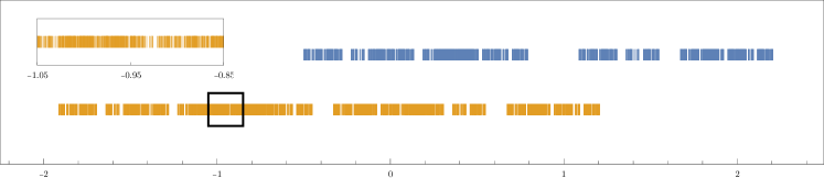
Figure 6. The windows $\widetilde{W}_{a}$ (blue/top) and $\widetilde{W}_{b}$ (yellow/bottom) for the tiling given by $\widetilde{\varrho}$. The inlay shows a stretched view of the marked region. Note that both windows are subsets of $\mathbb{R}\hskip 0.5pt$ and measure-theoretically disjoint, though this is almost impossible to illustrate due to the large Hausdorff dimension of their boundaries.

The diffraction measure of $\widetilde{\varLambda}=\widetilde{\varLambda}_{a}\,\dot{\cup}\,\widetilde{\varLambda}_{b}$ with weights $\alpha,\beta\in\mathbb{C}$, as above, reads

$$\widehat{\gamma}\,=\,\sum_{k\in L^{\circledast}}\bigl{|}\alpha A_{\widetilde{\varLambda}_{a}}(k)+\beta A_{\widetilde{\varLambda}_{b}}(k)\bigr{|}^{2}\delta_{k}$$

with the same Fourier module $L^{\circledast}$ as before and the non-zero FB coefficients read for all $k\in L^{\circledast}$ and $i\in\{a,b\}$

$$A_{\widetilde{\varLambda}_{i}}(k)\,=\,\widetilde{H}_{i}(k^{\star})$$

with $\widetilde{H}_{i}(k_{\mathrm{int}})=\tfrac{\operatorname{dens}(\widetilde{\varLambda})}{\operatorname{vol}(\widetilde{W})}\ \widecheck{\bm{1}_{\,\widetilde{W}_{i}}}\,(k_{\mathrm{int}})$. It is difficult to calculate the Fourier transform of sets like $\widetilde{W}_{i}$, which are Rauzy fractals. Fortunately, there exists a method due to Baake and Grimm [6] based on a cocycle approach. One defines the internal Fourier cocycle, which is a matrix cocycle induced by the inflation as follows. First, consider the inverse Fourier transform of the matrix of Dirac measures at positions given by the entries of $\widetilde{T}^{\star}$. For $k_{\mathrm{int}}\in\mathbb{R}\hskip 0.5pt_{\mathrm{int}}$, the matrix elements are defined by

$$\underline{B}_{ij}(k_{\mathrm{int}})\,=\,\sum_{t\in\widetilde{T}_{ij}}\,\mathrm{e}^{2\pi\mathrm{i}t^{\star}k_{\mathrm{int}}},$$

which is abbreviated as $\underline{B}(k_{\mathrm{int}})=\widecheck{\delta_{\widetilde{T}^{\star}}}$. For $\widetilde{\varrho}$, we have

$$\underline{B}(k_{\mathrm{int}})\,=\,\begin{pmatrix}\,\mathrm{e}^{4\pi\mathrm{i}k_{\mathrm{int}}}&1\\[2.84526pt] 1+\,\mathrm{e}^{2\pi\mathrm{i}k_{\mathrm{int}}}&\,\mathrm{e}^{-2\pi\mathrm{i}k_{\mathrm{int}}\sqrt{2}}\end{pmatrix}\hskip 0.5pt,$$

where $\underline{B}(0)$ is the substitution matrix of $\widetilde{\varrho}$. Now, one defines the matrix cocycle for $n\in\mathbb{N}$ via

$$\underline{B}^{(n)}(k_{\mathrm{int}})\,\mathrel{\mathop{:}}=\,\underline{B}(k_{\mathrm{int}})\,\underline{B}(\lambda^{\star}k_{\mathrm{int}})\,\cdots\,\underline{B}\bigl{(}(\lambda^{\star})^{n-1}k_{\mathrm{int}}\bigr{)},$$

and, further, one considers the matrix function $C(k_{\mathrm{int}})$

(2.18) $$C(k_{\mathrm{int}})\,\mathrel{\mathop{:}}=\,\lim_{n\to\infty}\lambda^{-n}\,\underline{B}^{(n)}(k_{\mathrm{int}}).$$

The function $C(k_{\mathrm{int}})$ is well defined and continuous, as the sequence $\bigl{(}\lambda^{-n}\underline{B}^{(n)}(k_{\mathrm{int}})\bigr{)}_{n}$ converges compactly on $\mathbb{R}\hskip 0.5pt$ [6, Thm. 4.6]. Moreover, the convergence of (2.18) is exponentially fast, which makes it effectively computable to any desired precision. Note that $C(k_{\mathrm{int}})$ is of rank smaller than or equal to $1$, so one can represent it as

$$C(k_{\mathrm{int}})\,=\,|\,c(k_{\mathrm{int}})\,\rangle\langle u|\hskip 0.5pt,$$

with the left PF eigenvector $\langle u|$ from (2.3). It turns out that the vector of functions $|\,c(k_{\mathrm{int}})\,\rangle$ has components

$$c_{i}(k_{\mathrm{int}})\,=\,\eta\,\widecheck{\bm{1}_{\,\widetilde{W}_{i}}}\,(k_{\mathrm{int}})\qquad\mbox{for some }\ \eta>0,$$

which provides the desired quantities; see [6, Sec. 4] for details.

(a) Equal weights $\alpha=\beta=1$.

(b) Weights $\alpha=\sqrt{2}$, $\beta=-1$.

Figure 7. Diffraction images of the model sets $\varLambda$ and $\widetilde{\varLambda}$, with two different choices of weights. (A) shows the case of equal weights, while (B) depicts the diffraction when the weights are chosen such that the central peak at $0$ vanishes. Both pictures show all Bragg peaks in positions $k\in L^{\circledast}\cap[0,5]$ with intensity $\geqslant 10^{-3}$.

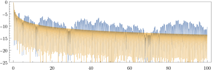
(a)

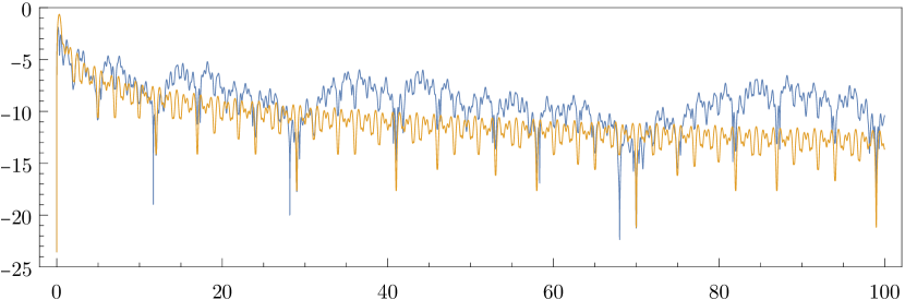
(b)

Figure 8. The functions $\log\bigl{(}|\widetilde{H}(k_{\mathrm{int}})k_{\mathrm{int}}|^{2}\bigr{)}$ (blue) and $\log\bigl{(}|H(k_{\mathrm{int}})|^{2}\bigr{)}$ (yellow) and their values for $k\in[0,100]$. The values are cropped at -25 for presentation purposes. Graph (A) shows the case with equal weights, whereas graph (B) depicts the case with $\alpha=\sqrt{2}$ and $\beta=-1$. Both graphs illustrate the slower decay of the intensities for the window with a boundary of non-trivial Hausdorff dimension.

Figure 2 compares the continuous counterparts of the intensity functions $|H(k_{\mathrm{int}})|^{2}$ and $|\widetilde{H}(k_{\mathrm{int}})|^{2}$ with equal weights $\alpha=\beta=1$ and Figure 7(a) shows the diffraction of both structures. On the level of intensities, one can recognise that the decay of $I_{\widetilde{\varLambda}}(k)$ is slower than that of $I_{\varLambda}(k)$, which supports the conjectured non-trivial relation between the boundary dimension of the window and the decay rate of the diffraction measure [21]. To illustrate the significantly slower decay, we include plots of the logarithms of the intensities on a larger scale in Figure 8(a). If the weights are chosen as $\alpha=\sqrt{2}$ and $\beta=-1$, the central peak vanishes. Figure 3 shows the diffraction intensities in such a case. Again, the slower decay can be observed as in the previous case (compare Figure 8(b)).

As above, we can recover the spectrum of the original symbolic sequence $\widetilde{w}$ by a reprojection. Since we are using the same CPS, the reprojection from (2.15) still applies, and Eq. (2.16) remains valid. The only difference is the method for obtaining the Fourier transform of the window. If the weights are both equal, one ends up with the lattice $(4-2\sqrt{2}\,)\mathbb{Z}$ as before. Figure 5 shows the diffraction of the deformed model sets $\varLambda^{\prime}$ and $\widetilde{\varLambda}^{\prime}$ with weights chosen so that the central peak vanishes.

At this point, we hope that the reader is well prepared to embark on the analogous programme in two dimensions, which we require to tackle the Hat and the Spectre tilings.

3. CAPs and Hats (and their relatives)

Recall that the Hat tiling, discovered by David Smith and his coauthors [31], is an aperiodic tiling of the plane using a disk-like prototile and its flipped version. Thus, it provides a partial solution to the monotile problem. In fact, there exists a continuum of monotiles related to the Hat, which have become known as the Hat family of tilings. Soon after this discovery, Baake, Gähler and Sadun [3] showed that all elements of this family give rise to topologically conjugate dynamical systems (up to scale and rotations). In the topological conjugacy class, there exists a self-similar relative of the Hat tiling called the CAP tiling. Further, they proved that the CAP tiling is MLD to a Euclidean model set and showed that the Hat tiling is a reprojection of the CAP tiling, as is every other member of the Hat family (after choosing an appropriate scale and orientation).

We aim to provide more details on these connections. In particular, we derive the explicit reprojection and deformation mappings. Then, using the cocycle approach, we calculate the diffraction and dynamical spectrum of the CAP tiling and, consequently, the spectra of the Hat tiling. Here, the cocycle method is required for this system because its window has some parts with fractal boundary. In what follows, we mimic the strategy of our one-dimensional guiding example from Section 2. Where possible, we keep an informal style and notation for better readability.

3.1. The embedding of the CAP tiling

Recall that the CAP tiling is built from 4 prototiles, each of which appears in 6 orientations. Therefore, there are altogether 24 prototiles up to translations. Figure 9(a) shows the substitution rule that can be turned into a proper stone inflation rule with fractiles [3, Fig. 3] and inflation factor $\tau^{2}$.

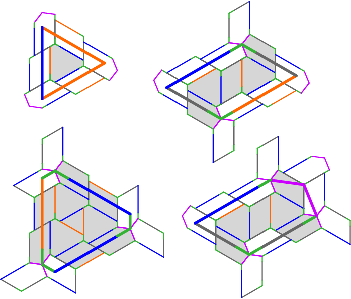
(a)

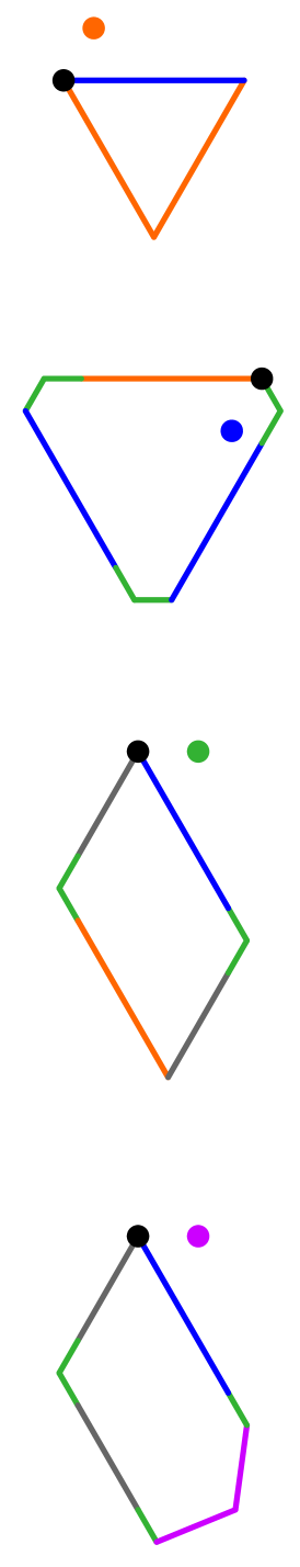
(b)

Figure 9. Panel (A) shows the inflation rule for the CAP tiling. Note that the grey polygons constitute the level-1 supertile, whereas the white ones are uniquely determined by the grey patch so that the inflation rule is border forcing. Panel (B) shows the position of the control point for every tile; see [3] for details.

Note that the control points of the tiles, as shown in Figure 9(b), do not all lie inside the tiles. They are chosen so that they form a single orbit under the translation action of the return module. In [3], it was derived that the return module is the principal ideal in the ring $\mathbb{Z}[\tau,\xi]$ generated by $(1-\xi)(\tau-\xi)$, with $\xi$ a primitive $6^{\mathrm{th}}$ root of unity. The return module (and hence the ideal $(1-\xi)(\tau-\xi)\,\mathbb{Z}[\tau,\xi]$, which equals $\tau^{2}(1-\xi)(\tau-\xi)\,\mathbb{Z}[\tau,\xi]=(3\tau+2-\xi)\,\mathbb{Z}[\tau,\xi]$ as $\tau$ is a unit) is generated by 4 elements,

(3.1) $$\begin{split}\bm{u}_{1}&\,=\,3\tau+2-\xi,\\ \bm{u}_{2}&\,=\,2\tau+1-\tau\xi+\xi,\\ \bm{u}_{3}&\,=\,1+3\tau\xi+\xi\,=\,\xi\bm{u}_{1},\\ \bm{u}_{4}&\,=\,\tau-1+\tau\xi+2\xi\,=\,\xi\bm{u}_{2}.\\ \end{split}$$

The module $\mathcal{R}_{{}_{\mathrm{CAP}}}=\mathbb{Z}\bm{u}_{1}\oplus\cdots\oplus\mathbb{Z}\bm{u}_{4}$ can be lifted via a Minkowski embedding into $\mathbb{R}\hskip 0.5pt^{4}\simeq\mathbb{C}^{2}$ to obtain the lattice $\mathcal{L}^{\prime}=\left\{(u,\,u^{\star})\,:\,u\in\mathcal{R}_{{}_{\mathrm{CAP}}}\right\}$, with a $\star$-map that follows from the Minkowski embedding. Let us explain this in more detail. The generating vectors of $\mathcal{L}^{\prime}$ constitute the columns of a matrix $V_{\mathbb{R}\hskip 0.5pt}\in\mathrm{Mat}(\mathbb{R}\hskip 0.5pt,4)$ or $V_{\mathbb{C}}\in\mathbb{C}^{2\times 4}$, which read

(3.2) $$V_{\mathbb{R}\hskip 0.5pt}\,=\,\frac{\raisebox{-2.0pt}{$1$}}{\raisebox{0.5pt}{$4$}}\begin{pmatrix}12+6\sqrt{5}&9+3\sqrt{5}&9+3\sqrt{5}&3+3\sqrt{5}\\[2.84526pt] -2\sqrt{3}&\sqrt{3}-\sqrt{15}&5\sqrt{3}+3\sqrt{15}&5\sqrt{3}+\sqrt{15}\\[2.84526pt] 12-6\sqrt{5}&9-3\sqrt{5}&9-3\sqrt{5}&3-3\sqrt{5}\\[2.84526pt] 2\sqrt{3}&-\sqrt{3}+\sqrt{15}&-5\sqrt{3}+3\sqrt{15}&-5\sqrt{3}+\sqrt{15}\end{pmatrix}$$

and

(3.3) $$V_{\mathbb{C}}\,=\,\begin{pmatrix}3\tau+2-\xi&2\tau+1-\tau\xi+\xi&1+3\tau\xi+\xi&\tau-1+\tau\xi+2\xi\\ -3\tau+4+\xi&-\tau+3-\tau\xi&-3\tau+5+3\tau\xi-4\xi&-2\tau+3+\tau\xi-3\xi\end{pmatrix},$$

respectively. We will tactically switch between the real and complex descriptions. Using the lattice $\mathcal{L}^{\prime}$, we obtain the CPS

(3.4) $$\begin{array}[]{ccccc@{}l}\mathbb{R}\hskip 0.5pt^{2}\simeq\mathbb{C}&\hskip-30.1388pt\xleftarrow{\quad\ \pi\ \quad}&\mathbb{R}\hskip 0.5pt^{2}\hskip-0.5pt\hskip-0.5pt\times\hskip-0.5pt\hskip-0.5pt\mathbb{R}\hskip 0.5pt^{2}_{\mathrm{int}}\simeq\mathbb{C}\hskip-0.5pt\hskip-0.5pt\times\hskip-0.5pt\hskip-0.5pt\mathbb{C}_{\mathrm{int}}&\xrightarrow{\quad\pi_{\text{int}}\quad}&\hskip-30.1388pt\mathbb{R}\hskip 0.5pt^{2}_{\mathrm{int}}\simeq\mathbb{C}_{\mathrm{int}}&\\ \cup&&\cup&&\hskip-34.44434pt\cup&\hskip-43.05542pt\raisebox{1.0pt}{\text{\scriptsize dense}}\\ \pi(\mathcal{L}^{\prime})&\hskip-30.1388pt\xleftarrow{\quad\hskip 0.5pt1:1\,\quad}&\mathcal{L}^{\prime}&\xrightarrow{\qquad\ \quad}&\hskip-30.1388pt\pi_{\text{int}}(\mathcal{L}^{\prime})&\\ \|&&&&\hskip-34.44434pt\|&\\ L=(3\tau{+}2{-}\xi)\,\mathbb{Z}[\tau,\xi]&\lx@intercol\hfil\hskip-34.44434pt\xrightarrow{\qquad\quad\quad\ \ \star\ \quad\quad\qquad}\hfil\lx@intercol&\hskip-30.1388pt{L}^{\star\hskip-0.5pt}=(-3\tau{+}4{+}\xi)\,\mathbb{Z}[\tau,\xi]&\end{array}$$

with the star map, in complex formulation, being given by

$$(a+b\tau+c\xi+d\tau\xi)^{\star}\,=\,a+b+c+d-(b+d)\tau-(c+d)\xi+d\tau\xi,\quad\mbox{for}\ a,b,c,d\in\mathbb{Q}\hskip 0.5pt.$$

This is the Galois isomorphism of $\mathbb{Q}(\tau,\xi)$ that fixes $\mathbb{Q}(\sqrt{-15}\hskip 0.5pt)$ but no other subfield of $\mathbb{Q}(\tau,\xi)$. In other words, the star map is a composition of the non-trivial algebraic conjugations in $\mathbb{Q}(\tau)$ and $\mathbb{Q}(\xi)$.

As in the guiding example, we construct the set-valued displacement matrix $T_{{}_{\mathrm{CAP}}}$, which is $24$-dimensional in this case. It has the block structure

(3.5) $$T_{{}_{\mathrm{CAP}}}\,=\,\begin{pmatrix}\varnothing&T_{12}&\varnothing&\varnothing\\ T_{21}&T_{22}&T_{23}&T_{24}\\ \varnothing&T_{32}&T_{33}&T_{34}\\ \varnothing&T_{42}&T_{43}&T_{44}\end{pmatrix},$$

where each entry represents a $6{\times}6$ matrix and $\varnothing$ is the $6{\times}6$ block of empty sets. The remaining matrices $T_{ij}$ are listed in Appendix A. As before, $T_{{}_{\mathrm{CAP}}}$ determines an IFS with linear scaling factor $\tau^{-1}$ on $\bigl{(}\mathcal{K}\mathbb{R}\hskip 0.5pt^{2}_{\mathrm{int}}\bigr{)}^{24}$, whose solution provides the windows for a model set which (possibly after removing points of density 0) is MLD with the CAP tiling, as discussed in detail in [3]. The total window and its subdivisions are shown in Figure 10.

Proposition 3.1 ([3]).

The CAP tiling is MLD with a Euclidean model set derived from the CPS (3.4) and the hexagonal window with fractal boundaries shown in Figure 10. ∎

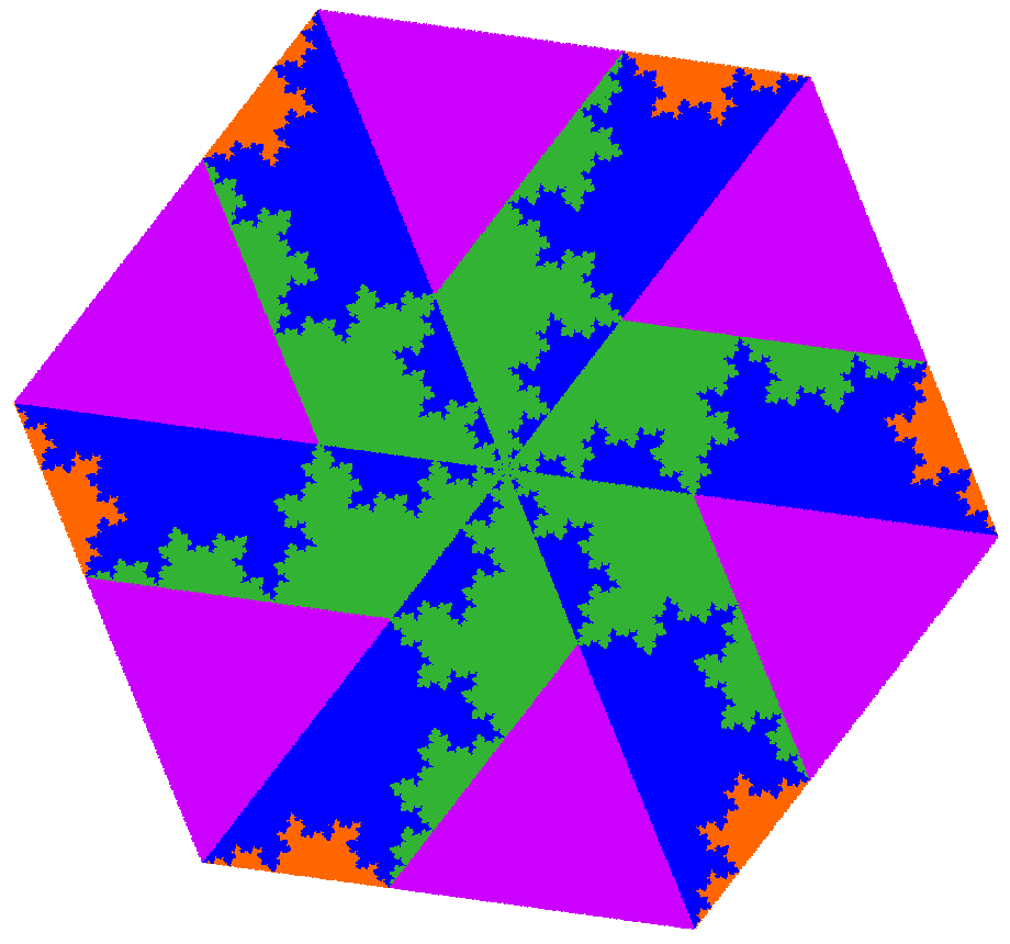
Figure 10. The window for the control points of the CAP tiling. The four different colours correspond to the four different shapes of prototiles. Note that there are two types of boundaries in the interior of the hexagon.

The total window is a hexagon rotated by $\arccos\bigl{(}\tfrac{3+\sqrt{5}}{4}\sqrt{\frac{3}{3\sqrt{5}+7}}\bigr{)}\approx 52.24^{\circ}$ relative to the window shown in [3], which is due to our choice of a basis. For the total window, it is possible to compute its Fourier transform explicitly. Nevertheless, since some of the subwindows have fractal boundary parts with Hausdorff dimension $\tfrac{\log(2+\sqrt{3})}{2\log(\tau)}\approx 1.3683764$, as shown in [3], one has to use the cocycle approach to obtain the FB coefficients for a general choice of weights. Thus, for all $k_{\mathrm{int}}\in\mathbb{R}\hskip 0.5pt^{2}_{\mathrm{int}}\simeq\mathbb{C}_{\mathrm{int}}$, we define the internal Fourier matrix $\underline{B}(k_{\mathrm{int}})$ as

(3.6) $$\underline{B}(k_{\mathrm{int}})_{ij}\,=\,\sum_{t\in T_{ij}}\,\mathrm{e}^{2\pi\mathrm{i}\langle t^{\star}|k_{\mathrm{int}}\rangle}\qquad\mbox{with}\ T=T_{{}_{\mathrm{CAP}}},$$

where $\langle\,\cdot\,|\,\cdot\,\rangle$ denotes the standard scalar product in $\mathbb{R}\hskip 0.5pt^{2}_{\mathrm{int}}$.

Since the tiles come in six orientations and the inflation rule respects the orientation, the displacement matrix as well as the (internal) Fourier matrix must reflect this fact. In particular, we have the following symmetry properties of the matrices $T_{{}_{\mathrm{CAP}}}$ and $\underline{B}(k_{\mathrm{int}})$.

Lemma 3.2.

For the displacement matrix $T_{{}_{\mathrm{CAP}}}$ and the corresponding internal Fourier matrix (3.6), one has the symmetry relations

$$S^{\top}\underline{B}(k_{\mathrm{int}})\,S\,=\,\underline{B}(\xi k_{\mathrm{int}})\quad\mbox{and}\quad S\,T_{{}_{\mathrm{CAP}}}\,S^{\top}\,=\,\xi\,T_{{}_{\mathrm{CAP}}}\hskip 0.5pt,$$

with the permutation matrix $S=\mathmybb{1}_{4}\,\otimes\,C\in\mathrm{Mat}\,(24,\mathbb{Z})$, where $\mathmybb{1}_{4}$ is the 4D identity matrix, $\otimes$ is the Kronecker product and $C$ stands for the companion matrix of $X^{6}-1$,

$$C\,=\,\left(\begin{smallmatrix}0&0&0&0&0&1\\ 1&0&0&0&0&0\\ 0&1&0&0&0&0\\ 0&0&1&0&0&0\\ 0&0&0&1&0&0\\ 0&0&0&0&1&0\end{smallmatrix}\right).$$

Proof.

The claims follow from the structure of the matrices and from an explicit computation using $\langle t^{\star}\,|\,\xi k_{\mathrm{int}}\rangle=\langle\xi^{-1}t^{\star}\,|\,k_{\mathrm{int}}\rangle=\langle(\xi t)^{\star}\,|\,k_{\mathrm{int}}\rangle$. ∎

This symmetry relation provides a good consistency check for numerical calculations, which can be implemented easily. It detects the position of eventual mistake; in particular, in $\underline{B}(k_{\mathrm{int}})$.

Now, we have all the ingredients needed to discuss the spectral properties of the CAP tiling. In [3, Lemma 10], it was proved that the CAP tiling is pure-point diffractive. The authors also derived the Fourier module

$$L^{\circledast}_{{}_{\mathrm{CAP}}}\,=\,\frac{\raisebox{-2.0pt}{$(1+\xi)(\tau-\xi)\hskip 0.5pt\mathrm{i}$}}{\raisebox{0.5pt}{$3\sqrt{15}$}}\,\mathbb{Z}[\tau,\xi],$$

which agrees with the dynamical spectrum of the CAP tiling dynamical system. For the diffraction intensities, it is sufficient to compute the Fourier transform of the windows using the cocycle. The result is shown in Figure 11. To obtain a first (and approximate) impression, one can replace the hexagonal total window with a circular one (of the same area) and use the explicit Fourier transform of a circle in terms of Bessel functions $J_{\nu}$; see [5, Rem. 9.15]. Note that the uncoloured CAP point set is not MLD with the coloured one, so it is insufficient to only work with the total window, as we demonstrate in Figures 11(a) and 11(b).

(a)

(b)

Figure 11. Diffraction pattern of the CAP tiling in the centred ball of radius 0.6, with two different sets of weights. The radii of the black disks are proportional to their intensities. Panel A shows the case with equal weights, where the intensity of the central peak equals $\operatorname{dens}(\varLambda_{{}_{\mathrm{CAP}}})^{2}=\tfrac{1}{75\tau^{4}}\approx 0.001945$. The diffraction exhibits the sixfold symmetry and mirror symmetries as well. The second brightest peaks are located at $\tfrac{1}{30}\bigl{(}\sqrt{5}+\mathrm{i}\sqrt{3}\,(5+2\sqrt{5}\,)\bigr{)}$ and all its $\xi$-multiples. Figure (B) shows the diffraction pattern for weights $(0,\,0,\,\tau,\,-1)$, chosen so that the central peak vanishes. The Bragg peaks are not as bright as in Figure (A), so in order to obtain a more visible pattern, we magnified all intensities by a factor of 4. One can still see the sixfold symmetry, but the mirror symmetry is broken, which demonstrates the chiral nature of the CAP tiling (as manifest in the window in Figure 10). To create the figure, 15 iterations of the cocycle were used.

3.2. Shape changes — from CAPs to Hats

Let us now explain the reprojection of the CAP tiling that results in the Hat tiling. To be more precise, we start with the (coloured) set of control points, which is MLD to the CAP tiling, and we modify it to a different coloured point set, which is MLD to the Hat tiling. This is then a deformed model set in the sense of [10, 11], which can now be used, as outlined in [3]. Moreover, the authors also derived the return module for the Hat tiling, which reads

(3.7) $$\frac{\raisebox{-2.0pt}{$\sqrt{5}$}}{\raisebox{0.5pt}{$4$}}(1+\xi)(\tau-\xi)^{3}\,\mathbb{Z}[\xi]\hskip 0.5pt.$$

It is a scaled and rotated triangular lattice, thus is of rank $2$ — in comparison to $\mathcal{R}_{{}_{\mathrm{CAP}}}$, which is of rank $4$. The generators for (3.7) can be chosen as

(3.8) $$\begin{split}\bm{v}_{1}&\,=\,\frac{\raisebox{-2.0pt}{$\sqrt{5}$}}{\raisebox{0.5pt}{$4$}}\xi(1+\xi)(\tau-\xi)^{3},\\ \bm{v}_{2}&\,=\,\frac{\raisebox{-2.0pt}{$\sqrt{5}$}}{\raisebox{0.5pt}{$4$}}\xi^{2}(1+\xi)(\tau-\xi)^{3}.\\ \end{split}$$

Let us derive the reprojection, and the deformation mapping from the CAP to the Hat tiling. First, we identify the generators of the return module of the CAP tiling (and due to our choice of the control points, we do not need to pay attention to the type of the points!), for example as indicated in Figure 12(a). Then, we find the corresponding patch in the Hat tiling and identify the same return vectors as shown in Figure 12(b). The reprojection is chosen so that all control points lie on the anti-Hats (meaning the reflected Hats), and their colouring determines the neighbourhood. Thus, the coloured point set is MLD with the Hat tiling.

(a)

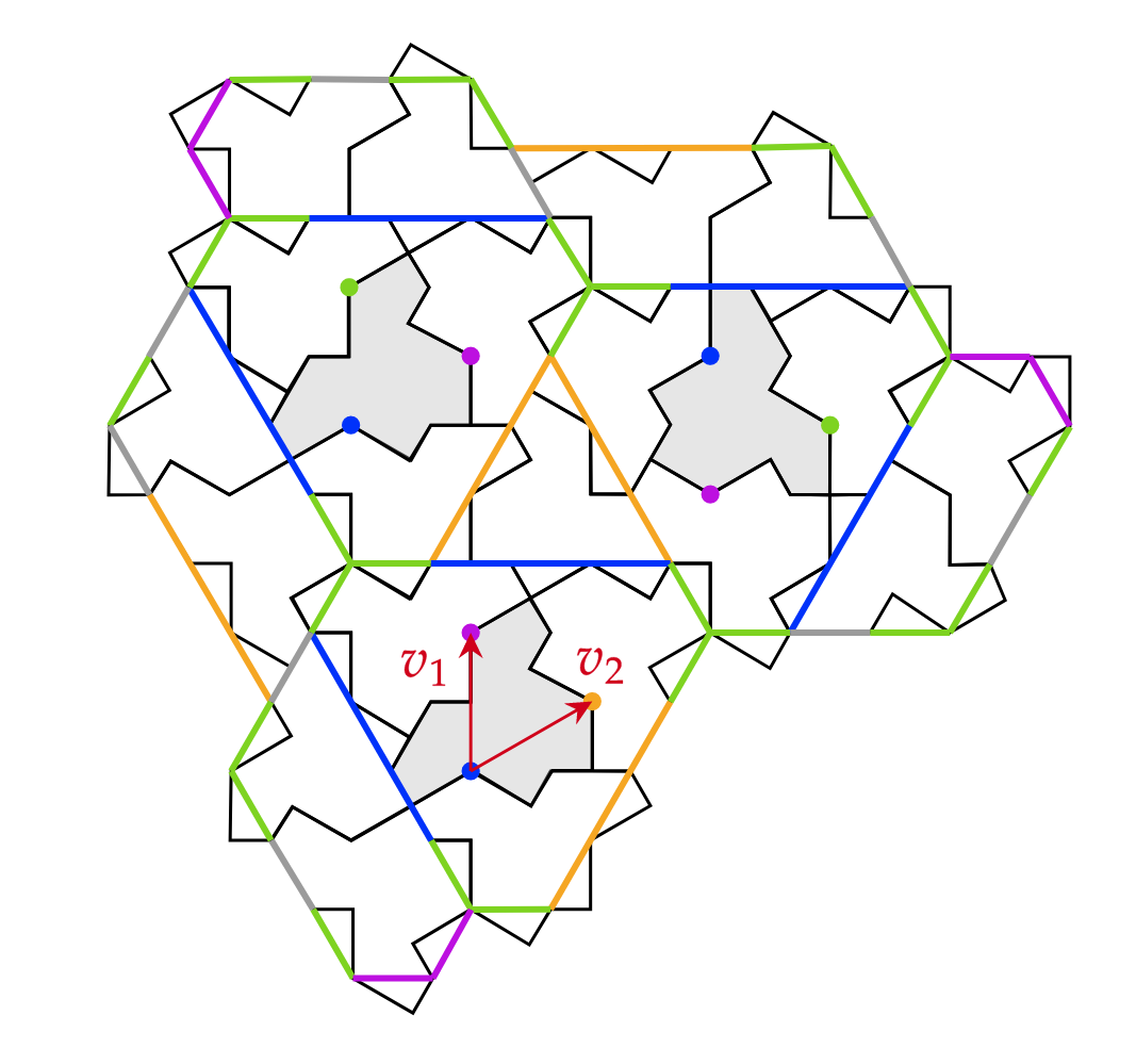
(b)

Figure 12. Patch of the CAP tiling with its control points (A). The 4 generators of the return module are indicated. Panel (B) shows the deformed version of the same patch together with the control points and the underlying Hat tiling. Note that one has to deform the tiles first, then identify the new return module, which is a triangular lattice in this case. Then, one can decide how to choose the control points accordingly. In our case, we decided to choose the control point so that they all lie on the anti-Hats as shown in Figure (B). We also include the generators of the return module of the Hat tiling and indicate the generators by arrows.

Now, the reprojection map acts on the level of the generators of the return modules as

$$\begin{split}\bm{u}_{1}&\longmapsto\ 3\bm{v}_{1}-\bm{v}_{2},\\ \bm{u}_{2}&\longmapsto\ \bm{v}_{1},\\ \bm{u}_{3}&\longmapsto\ \bm{v}_{1}+2\bm{v}_{2},\\ \bm{u}_{4}&\longmapsto\ \bm{v}_{2}.\\ \end{split}$$

This determines the entire reprojection. As in our guiding example, we can thus employ the matrix description via the reprojection matrix $\pi^{\prime}\in\mathbb{R}\hskip 0.5pt^{2\times 4}\simeq\mathbb{C}^{1\times 2}$, acting on the lattice generators as

$$\pi^{\prime}\,V_{\mathbb{C}}\,=\,\bigl{(}\begin{matrix}3\bm{v}_{1}-\bm{v}_{2}&\bm{v}_{1}&\bm{v}_{1}+2\bm{v}_{2}&\bm{v}_{2}\end{matrix}\bigr{)},$$

or the real version

(3.9) $$\pi^{\prime}\,V_{\mathbb{R}\hskip 0.5pt}\,=\,\frac{\raisebox{-2.0pt}{$1$}}{\raisebox{0.5pt}{$16$}}\begin{pmatrix}15+45\sqrt{5}&18\sqrt{5}&45+9\sqrt{5}&15+9\sqrt{5}\\[2.84526pt] -25\sqrt{3}+9\sqrt{15}&-10\sqrt{3}&-5\sqrt{3}+27\sqrt{15}&-5\sqrt{3}+9\sqrt{15}\end{pmatrix}.$$

Since $V_{\mathbb{R}\hskip 0.5pt}$ is an invertible matrix, one can multiply (3.9) from the right by $V^{-1}_{\mathbb{R}\hskip 0.5pt}$ to obtain

$$\pi^{\prime}\,=\,\begin{pmatrix}1&0&-\frac{11}{16}&\frac{3\sqrt{15}}{16}\\[5.69054pt] 0&1&\frac{3\sqrt{15}}{16}&\frac{11}{16}\end{pmatrix}.$$

Since the reprojection can be considered as a special case of a deformation of a model set, we have $\bm{v}_{i}\,=\,\bm{u}_{i}+D\bm{u}^{\star}_{i}$, for $i\in\{1,2,3,4\}$, where $D$ is the desired deformation mapping form $\mathbb{R}\hskip 0.5pt^{2}_{\mathrm{int}}$ to $\mathbb{R}\hskip 0.5pt^{2}$. Again, this can be rewritten compactly using the matrices and for the real version, then giving $\pi^{\prime}\,=\,\pi+D\pi_{\mathrm{int}}$. The projections with respect to the standard basis read $\pi=\bigl{(}\begin{smallmatrix}1&0&0&0\\ 0&1&0&0\end{smallmatrix}\bigr{)}$ and $\pi_{\mathrm{int}}=\bigl{(}\begin{smallmatrix}0&0&1&0\\ 0&0&0&1\end{smallmatrix}\bigr{)}$, so

$$D\,=\,\frac{\raisebox{-2.0pt}{$1$}}{\raisebox{0.5pt}{$16$}}\begin{pmatrix}-11&3\sqrt{15}\\[2.84526pt] 3\sqrt{15}&11\end{pmatrix}.$$

We summarise the above derivation as follows.

Theorem 3.3.

The set of control points of the Hat tiling is a deformed model set obtained from the control points of the CAP tiling using

$$D\,=\,\frac{\raisebox{-2.0pt}{$1$}}{\raisebox{0.5pt}{$16$}}\begin{pmatrix}-11&3\sqrt{15}\\[2.84526pt] 3\sqrt{15}&11\end{pmatrix}$$

as the linear deformation mapping. Moreover, the Hat control points are a reprojection of the CAP tiling control points using the projection $\pi^{\prime}\,=\,\pi+D\pi_{\mathrm{int}}$. ∎

The matrix $D$ allows the computation of the diffraction of the Hat tiling from the amplitude functions of the CAP tiling. It plays a role similar to the scaling factor $\lambda^{-2}$ in our guiding example, now with $D:\mathbb{R}\hskip 0.5pt^{2}_{\mathrm{int}}\to\mathbb{R}\hskip 0.5pt^{2}$.

Let us now move to the spectral properties of the Hat tiling. Due to the topological conjugacy, its Fourier module is the same as that of the CAP tiling, namely $L^{\circledast}_{{}_{\mathrm{CAP}}}$. It (of course) contains the dual of the return module of the Hat tiling, which is

(3.10) $$\frac{\raisebox{-2.0pt}{$(1+\xi)(\tau-\xi)^{3}\,\mathrm{i}$}}{\raisebox{0.5pt}{$3\sqrt{15}$}}\,\mathbb{Z}[\xi]\hskip 0.5pt.$$

$L^{\circledast}_{{}_{\mathrm{CAP}}}$ gives the dynamical spectrum of the Hat tiling.

Further, one has an additional similarity to the one-dimensional guiding example. As already suggested by the return module (3.7), the set of control points of the Hat tiling forms a subset of the triangular lattice. It follows from [5, Thm. 10.3] that the corresponding diffraction measure is lattice-periodic. The lattice of periods is the dual of the underlying lattice. In our case, it is given by (3.10).

Since we already know the dynamical spectrum of the Hat tiling, we can proceed to compute the FB coefficients. Suppose that tiles of type $i$ come with weight $\alpha_{i}\in\mathbb{C}$. Then, the FB coefficients vanish for $k\notin L^{\circledast}_{{}_{\mathrm{CAP}}}$, while the remaining ones are given via the inverse Fourier transform of the windows as

(3.11) $$A_{{}_{\mathrm{Hat}}}(k)\,=\,H_{{}_{\mathrm{CAP}}}(k^{\star}-D^{\top}k),$$

with

$$H_{{}_{\mathrm{CAP}}}(k_{\mathrm{int}})\,=\,\frac{\operatorname{dens}\bigl{(}\varLambda_{{}_{\mathrm{CAP}}}\bigr{)}}{\operatorname{vol}\bigl{(}W_{{}_{\mathrm{CAP}}}\bigr{)}}\sum_{i}\alpha_{i}\hskip 0.5pt\widecheck{\bm{1}_{W_{{}_{\mathrm{CAP},i}}}}\bigl{(}k_{\mathrm{int}}\bigr{)},$$

where $W_{{}_{\mathrm{CAP},i}}$ stands for the part of the window from Fig. 10 corresponding to points of type $i$.

Note that the set of arguments $\{k^{\star}-D^{\top}k\,:\,k\in L^{\circledast}\}$ forms a lattice in $\mathbb{R}\hskip 0.5pt^{2}_{\mathrm{int}}$ — in contrast to $L^{\circledast}_{{}_{\mathrm{CAP}}}$ itself, which is a dense subset of $\mathbb{R}\hskip 0.5pt^{2}$. The lattice is $\tfrac{1}{12}(\tau-2+3\xi)\hskip 0.5pt\mathbb{Z}[\xi]$ and provides additional insight into the periodic nature of the diffraction measure. Figure 13 shows the diffraction spectra of the Hat tiling with two different sets of weights, together with a fundamental domain and generators of the lattice of periods.

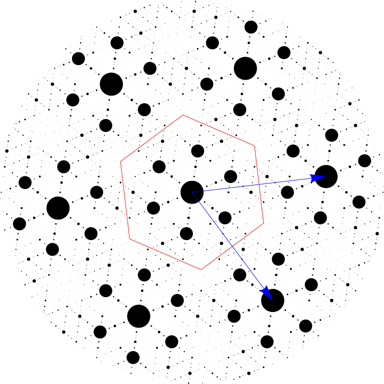
(a)

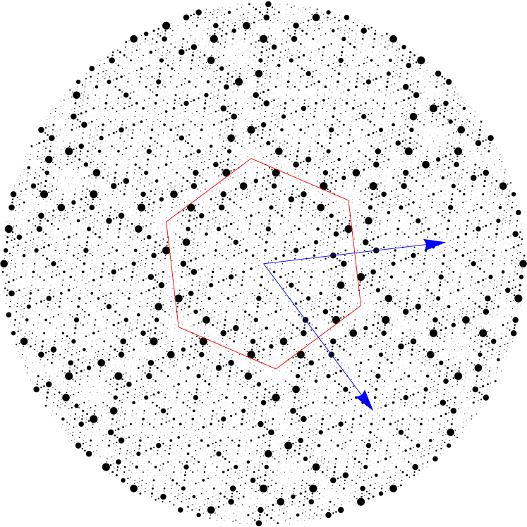
(b)

Figure 13. Diffraction of the Hat tiling with equal weights (A), and with weights $(0,\,0,\,\tau,-1)$ chosen such that the central peak vanishes (B). Both pictures show a fundamental domain (hexagon) of the support of the diffraction measure, which is lattice-periodic with periods (3.10). Two fundamental periods are indicated by the blue arrows. The intensities of the Bragg peaks are proportional to the area of the disks, and the intensity of the brightest one in (A) is $\tfrac{1}{75\tau^{4}}\approx 0.001945$. In both cases, one has sixfold symmetry, while the absence of any mirror symmetry can be seen in the fundamental domain. $15$ iterations of the cocycle were used in the computation.

The formula for the FB coefficients (3.11) holds for the entire class of deformations, among them all affine ones. The proof mimics the one given for the one-dimensional silver mean case in (2.16). We state it as a theorem for linear maps (the translation part of affine mappings adds an additional phase factor, which does not play a role for the intensities); it can also be found implicitly in a slightly different form in [11, Thm. 2.6].

Theorem 3.4.

Let $\varLambda\subset\mathbb{R}\hskip 0.5pt^{n}$ be a model set arising from a Euclidean CPS $(\mathbb{R}\hskip 0.5pt^{n},\,\mathbb{R}\hskip 0.5pt^{n}_{\mathrm{int}},\,\mathcal{L})$ with window $W$, and let $\vartheta:\mathbb{R}\hskip 0.5pt^{n}_{\mathrm{int}}\longrightarrow\mathbb{R}\hskip 0.5pt^{n}$ be a linear mapping, represented by the matrix $D$ with respect to the standard bases in $\mathbb{R}\hskip 0.5pt^{n}_{\mathrm{int}}$ and $\mathbb{R}\hskip 0.5pt^{n}$. Then, for $k\in L^{\circledast}$, the FB coefficients $A_{\varLambda_{\vartheta}}(k)$ of the deformed model set $\varLambda_{\vartheta}=\{x+\vartheta(x^{\star})\,:\,x\in\varLambda\}$ are given by

$$A_{\varLambda_{\vartheta}}(k)\,=\,H(k^{\star}-D^{\top}k),$$

with

$$H(k_{\mathrm{int}})\,=\,\frac{\operatorname{dens}(\varLambda)}{\operatorname{vol}(W)}\,\hskip 0.5pt\widecheck{\bm{1}_{W}}\bigl{(}k_{\mathrm{int}}\bigr{)}.\qed$$

4. Spectre

The Spectre tiling was constructed shortly after the discovery of the Hat tiling by the same team of authors [32]. The Spectre, which looks a little like a malicious cat, is an aperiodic monotile with respect to translations and rotations. Notably, in contrast to the Hat tiling, a reflected copy of the prototile is not required. The Hat and Spectre tilings are closely related, as the latter was constructed using two tiles from the Hat tiling family. Nevertheless, the combinatorics of the Spectre is rather different from that of the Hat.

Despite the fact that one needs only translations and rotations of a single Spectre tile, the Spectre tiling forms two LI-classes. This manifests itself in distinct (and rationally independent) frequencies for Spectres rotated by $\tfrac{\pi}{6}$ relative to each other. Although Spectres occur in 12 orientations, the LI-classes have six-fold symmetry only. It is thus tempting to speak of Spectres and Shadow-Spectres, whose frequency ratio is $(4+\sqrt{15})^{2}$.

Smith et al. [32] provided a combinatorial inflation for marked hexagons, which gives rise to the Spectre tiling. This inflation acts on nine different hexagons ($\Gamma,\,\Delta,\,\Theta,\,\Lambda,\,\Xi,\,\Pi,\,\Sigma,\,\Phi,\,\Psi$), each appearing in six different orientations, which gives 54 translational prototiles in total. One can assign control points to five of them ($\Theta,\,\Xi,\,\Sigma,\,\Phi,\,\Psi$) such that the resulting point set is MLD to the Spectre tiling. Moreover, based on the combinatorial inflation, a self-similar version of the Spectre tiling was derived [2], called CASPr. It is topologically conjugate (but not MLD) to the Spectre, and it possesses a model set description, which we employ in what follows. The cut-and-project description of the CASPr tiling is more complex than that of the CAP tiling, which plays the analogous role for the Hat tiling [3]. Although the leading eigenvalue of the inflation matrix is $\lambda=4+\sqrt{15}$, a PV unit, the corresponding linear scaling is $\sqrt{4+\sqrt{15}}$. Due to the chiral nature of the tiling, a reflection is required when the substitution rule is applied once; see [2] for further details. The underlying number field is the quartic number field $\mathbb{Q}(\xi,\lambda)=\mathbb{Q}(\alpha)$ with $\alpha=\sqrt{5}\,\mathrm{e}^{\frac{2\pi\mathrm{i}}{12}}$, which satisfies $\alpha^{4}=5\alpha^{2}-25$. In contrast to the Hat tiling, $\mathbb{Q}(\alpha)$ has class number 2, see entry 4.0.3600.3 of [18], which makes the description of the return module in terms of ideals more difficult.

The generators of the return module $\mathcal{R}_{{}_{\mathrm{CASPr}}}$ can be chosen as follows

(4.1) $$\begin{split}g_{1}\ &=\ -1-\xi+\lambda-2\xi\lambda,\\ g_{2}\ &=\ 1-2\xi+2\lambda+\xi\lambda\ =\ \xi\hskip 0.5ptg_{1},\\ g_{3}\ &=\ -2+\xi+2\lambda+2\xi\lambda,\\ g_{4}\ &=\ -2-2\xi-\lambda+2\xi\lambda,\end{split}$$

so $\mathcal{R}_{{}_{\mathrm{CASPr}}}\subset\mathbb{Z}[\lambda,\xi]$, the latter being of index $3$ in the ring of integers $\mathcal{O}_{\mathbb{Q}(\alpha)}=\langle 1,\,\alpha,\,\tfrac{\alpha^{2}}{5},\,\tfrac{\alpha^{3}}{5}\rangle$. Note that, although $\mathbb{Z}[\lambda,\xi]$ is not an ideal in $\mathcal{O}_{\mathbb{Q}(\alpha)}$, the return module $\mathcal{R}_{{}_{\mathrm{CASPr}}}$ is an ideal in $\mathbb{Z}[\lambda,\xi]$ as well as in $\mathcal{O}_{\mathbb{Q}(\alpha)}$. Surprisingly, it possesses the same set of generators in both cases, so we can write (without confusion)

(4.2) $$\mathcal{R}_{{}_{\mathrm{CASPr}}}\,=\,\bigl{(}g_{1},\,g_{3}\bigr{)}\,=\,\bigl{(}g_{1}\bigr{)}+\bigl{(}g_{3}\bigr{)}.$$

The representation of $\mathcal{R}_{{}_{\mathrm{CASPr}}}\subset\mathbb{Z}[\lambda,\xi]$ in $\mathbb{R}\hskip 0.5pt^{2}$ can be chosen as

(4.3) $$\begin{split}1\ &\longmapsto\ \bm{w}_{1}\,=\,\biggl{(}\begin{matrix}1\\ 0\end{matrix}\biggr{)}\,,\\ \xi\ &\longmapsto\ \bm{w}_{2}\,=\,\frac{\raisebox{-2.0pt}{$1$}}{\raisebox{0.5pt}{$2$}}\biggl{(}\begin{matrix}1\\ \sqrt{3}\end{matrix}\biggr{)}\,,\\ \lambda\ &\longmapsto\ \bm{w}_{3}\,=\,\biggl{(}\begin{matrix}4+\sqrt{15}\,\\ 0\end{matrix}\biggr{)}\,=\,\lambda\bm{w}_{1},\\ \xi\lambda&\longmapsto\ \bm{w}_{4}\,=\,\frac{\raisebox{-2.0pt}{$1$}}{\raisebox{0.5pt}{$2$}}\biggl{(}\begin{matrix}4+\sqrt{15}\\ 4\sqrt{3}+3\sqrt{5}\end{matrix}\biggr{)}\,=\,\lambda\bm{w}_{2}.\end{split}$$

With this parametrisation, the expansive mapping of the inflation rule reads

$$R\,=\,\frac{\raisebox{-2.0pt}{$1$}}{\raisebox{0.5pt}{$6$}}\begin{pmatrix}9+2\sqrt{15}&-\sqrt{3}\\ -\sqrt{3}&-9-2\sqrt{15}\end{pmatrix}\!.$$

It can be understood as a concatenation of the reflection about the $x$-axis, a rotation by $\theta=-\arccos\bigl{(}\tfrac{9+2\sqrt{15}}{6\sqrt{\lambda}}\bigr{)}\approx-5.9^{\circ}$, and a linear scaling by $\sqrt{\lambda}$. As such, $R$ is a matrix square root of $\lambda\hskip 0.5pt\mathmybb{1}_{2}$.

The $\star$-images of the generators $\bm{w}_{i}$ are given by the embedding of $1$, $\overline{\xi}$, $\lambda^{\prime}$ and $\overline{\xi}\lambda^{\prime}$, where $\overline{\,\cdot\,}$ denotes complex conjugation and ${}^{\prime}:\mathbb{Q}(\lambda)\to\mathbb{Q}(\lambda)$ is the non-trivial field automorphism $(a+b\lambda)^{\prime}\mapsto a+8b-b\lambda$. The concatenation of these two maps defines the $\star$-map in $\mathbb{Q}(\lambda,\xi)$, which is the non-trivial Galois isomorphism fixing the subfield $\mathbb{Q}(\sqrt{-5}\hskip 0.5pt)$ of $\mathbb{Q}(\lambda,\xi)$. For the embedding of the generators, we obtain

(4.4) $$\begin{split}\bm{w}^{\star}_{1}\ &=\,\biggl{(}\begin{matrix}1\\ 0\end{matrix}\biggr{)}\,,\\ \bm{w}^{\star}_{2}\ &=\,\frac{\raisebox{-2.0pt}{$1$}}{\raisebox{0.5pt}{$2$}}\biggl{(}\begin{matrix}1\\ -\sqrt{3}\end{matrix}\biggr{)}\,,\\ \bm{w}^{\star}_{3}\ &=\,\biggl{(}\begin{matrix}4-\sqrt{15}\\ 0\end{matrix}\biggr{)}\,,\\ \bm{w}^{\star}_{4}\ &=\,\frac{\raisebox{-2.0pt}{$1$}}{\raisebox{0.5pt}{$2$}}\biggl{(}\begin{matrix}4-\sqrt{15}\\ -4\sqrt{3}+3\sqrt{5}\end{matrix}\biggr{)}\,,\end{split}$$

which describes the entire $\star$-map due to $\mathbb{Q}$-linearity. The induced matrix $R^{\star}$ becomes

$$R^{\star}\,=\,\frac{\raisebox{-2.0pt}{$1$}}{\raisebox{0.5pt}{$6$}}\begin{pmatrix}9-2\sqrt{15}&\sqrt{3}\\ \sqrt{3}&-9+2\sqrt{15}\end{pmatrix}\!,$$

and is a matrix square root of $\lambda^{\star}\hskip 0.5pt\mathmybb{1}_{2}$.

Using this embedding, one obtains a Euclidean CPS with the lattice given by the embedding of the return module (4.3). Its basis matrix reads

(4.5) $$B\,=\,\frac{\raisebox{-2.0pt}{$3$}}{\raisebox{0.5pt}{$2$}}\begin{pmatrix}-1&-5-\sqrt{15}&7+2\sqrt{15}&-2\\[2.0pt] -3\sqrt{3}-2\sqrt{5}&-\sqrt{3}-\sqrt{5}&3\sqrt{3}+2\sqrt{5}&2\sqrt{3}+2\sqrt{5}\\[2.0pt] -1&-5+\sqrt{15}&7-2\sqrt{15}&-2\\[2.0pt] 3\sqrt{3}-2\sqrt{5}&\sqrt{3}-\sqrt{5}&-3\sqrt{3}+2\sqrt{5}&-2\sqrt{3}+2\sqrt{5}\end{pmatrix}.$$

The lattice has density $\tfrac{1}{3645}$. Via the form (4.4), one can take the $\star$-image of the tiling control points to obtain the windows. Moreover, the control points satisfy renormalisation equations as in the previous examples. In this case, we obtain 54 equations for 54 point sets, 30 of which then give the window, see [2] for further details.

The total window is simply connected, with sixfold symmetry, but without any mirror symmetry. It has fractal boundaries and, in contrast to the Hat tiling, there are no other types of boundaries. The window is shown in Figure 14.

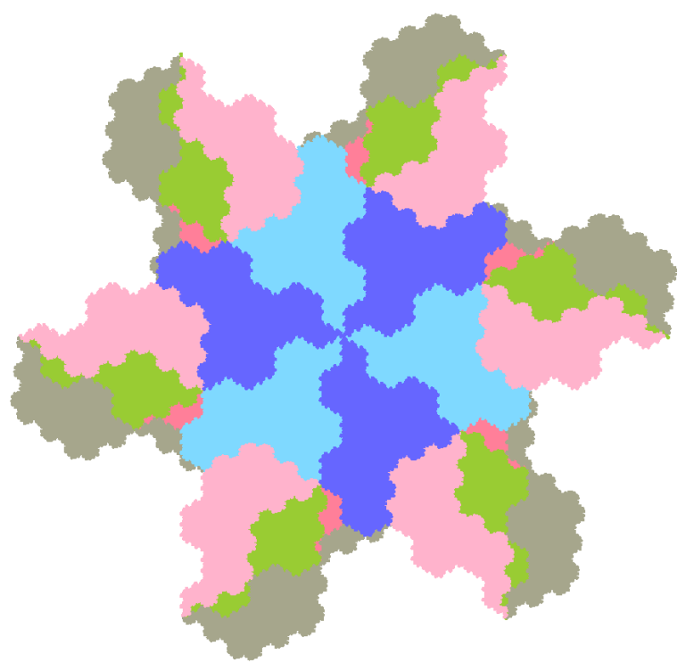
Figure 14. The window for the control points of the Spectre tiling. The five different colours correspond to the five different types of control points. We used two shades of blue to visualise the six different regions in the central blue part. The window has sixfold symmetry, but no mirror symmetry.

Since the window is a fundamental domain of a hexagonal lattice in $\mathbb{R}\hskip 0.5pt^{2}_{\mathrm{int}}$, its volume is easily computable [2] and reads $\tfrac{135}{2}(4\sqrt{3}-3\sqrt{5}\,)\approx 14.85$. By a density argument [28], we know that the control points of the CASPr tiling form a subset of the model set with window from Figure 14, where both have the same density. This tiny difference stems from boundary points of the window and does not affect the FB coefficients. This also implies that the diffraction and dynamical spectra of the Spectre tiling are both pure point [2].

Proposition 4.1 ([2]).

The CASPr tiling is MLD with a Euclidean model set derived from the CPS arising from the Minkowski embedding of $\mathcal{R}_{{}_{\mathrm{CASPr}}}$ and the window with fractal boundaries shown in Figure 14. ∎

Figure 15. Diffraction of the CASPr tiling control points with equal weights. The picture shows a disk of radius 0.5 around $k=0$. The intensities of the Bragg peaks are proportional to the area of the disks and the intensity of the brightest one equals $\tfrac{31-8\sqrt{15}}{972}\approx 0.000016597\dots$. One has sixfold rotational symmetry, but no reflection symmetry. $15$ iterations of the cocycle were used for the computation.

Now, for the Fourier module (and the dynamical spectrum), one considers the dual basis matrix $B^{\ast}=\bigl{(}B^{-1}\bigr{)}^{\top}$ of (4.5) and its $\pi$-projection. The generators written as columns of a matrix read

$$\frac{\raisebox{-2.0pt}{$1$}}{\raisebox{0.5pt}{$90$}}\begin{pmatrix}-5+2\sqrt{15}&-10+2\sqrt{15}&-5+2\sqrt{15}&-5+\sqrt{15}\\[2.0pt] -5\sqrt{3}+2\sqrt{5}&10\sqrt{3}-8\sqrt{5}&5\sqrt{3}-4\sqrt{5}&-5\sqrt{3}+5\sqrt{5}\end{pmatrix},$$

and the Fourier module $L^{\circledast}_{{}_{\mathrm{CASPr}}}$ (the dynamical spectrum) can be expressed as

$$L^{\circledast}_{{}_{\mathrm{CASPr}}}\,=\,\frac{\raisebox{-2.0pt}{$\mathrm{i}\sqrt{5}$}}{\raisebox{0.5pt}{$135$}}\hskip 0.5pt\mathcal{R}_{{}_{\mathrm{CASPr}}}\hskip 0.5pt,$$

with $\mathcal{R}_{{}_{\mathrm{CASPr}}}$ from (4.2), so it forms a fractional ideal. We refer the reader to [2] for further details and a number-theoretic description of the return and Fourier modules.

For the diffraction amplitudes, we again employ the cocycle method. This time, the displacement matrix has size $54\times 54$, but since several metatiles form clusters, one can reduce the dimension to $30\times 30$, see [2] for further details.

For the total intensity, one has to consider the weighted sum, so one obtains

$$I_{{}_{\mathrm{CASPr}}}(k)\,=\,\begin{cases}\bigl{|}H_{{}_{\mathrm{CASPr}}}(k^{\star})\bigr{|}^{2},&\mbox{if}\ k\in L^{\circledast}_{{}_{\mathrm{CASPr}}},\\ 0,&\mbox{otherwise,}\end{cases}$$

with

$$H_{{}_{\mathrm{CASPr}}}(k_{\mathrm{int}})\,=\,\frac{\operatorname{dens}\bigl{(}\varLambda_{{}_{\mathrm{CASPr}}}\bigr{)}}{\operatorname{vol}\bigl{(}W_{{}_{\mathrm{CASPr}}}\bigr{)}}\sum_{i}\alpha_{i}\hskip 0.5pt\widecheck{\bm{1}_{W_{{}_{\mathrm{CASPr},i}}}}\bigl{(}k_{\mathrm{int}}\bigr{)},$$

where $\alpha_{i}\in\mathbb{C}$ denotes the weight of tiles of type $i$. We note that, in order to obtain the diffraction intensities, one only has to choose non-zero weights for $30$ (instead of $54$) elements. The diffraction pattern for equal weights (near $0$) is shown in Figure 15. It reflects the properties of the Spectre tiling: It exhibits sixfold rotational symmetry, while mirror symmetry is absent.

The CASPr tiling can be reprojected, and various tilings related to the Spectre tiling can be obtained. First, we start by recovering a tiling by regular hexagons, which is combinatorially equivalent to the tiling by Spectre clusters and plays a pivotal role in all cohomological considerations in [2]. The deformation matrix reads

(4.6) $$D_{{}_{\mathrm{hex}}}\,=\,\begin{pmatrix}-1&0\\ 0&1\end{pmatrix},$$

and the new return module becomes a scaled and rotated hexagonal lattice of rank $2$ (as one would expect from a hexagonal tiling),

$$\mathcal{R}_{{}_{\mathrm{hex}}}\,=\,6\hskip 0.5pt\mathrm{i}\sqrt{5}\,\mathbb{Z}[\xi]\,=\,(8-16\xi-2\lambda+4\lambda\xi)\,\mathbb{Z}[\xi]\hskip 0.5pt.$$

The reprojection of the generators $g_{i}$ is shown in Figure 16(a). We note at this point that the resulting tiling consists of combinatorial hexagons (which are not regular hexagons, but geometrical shapes rather similar to the CASPr tiles, see [2, Fig. 9]), but within the MLD class of this tiling, one also finds a tiling with regular hexagons.

(a)

(b)

Figure 16. Reprojected generators $g_{i}$ (Eq. (4.1)) of the return module of the CASPr tiling. Figure (A) shows the deformation to the regular hexagon tiling and the underlying lattice $6\hskip 0.5pt\mathrm{i}\sqrt{5}\,\mathbb{Z}[\xi]$ (red dots). Figure (B) shows the generators for the Hat–Turtle tiling and the lattice $\tfrac{2}{67}\bigl{(}-185-206\xi+20\lambda+44\lambda\xi\bigr{)}\mathbb{Z}[\xi]$.

This implies that the control points form a lattice subset, and hence the diffraction image is lattice-periodic with the lattice of periods being given by $\mathcal{R}^{\ast}_{{}_{\mathrm{hex}}}$

(4.7) $$\mathcal{R}^{\ast}_{{}_{\mathrm{hex}}}\,=\,\frac{\raisebox{-2.0pt}{$\sqrt{15}$}}{\raisebox{0.5pt}{$45$}}\,\mathbb{Z}[\xi]\,=\,\frac{\raisebox{-2.0pt}{$\lambda-4$}}{\raisebox{0.5pt}{$45$}}\,\mathbb{Z}[\xi]\hskip 0.5pt.$$

We illustrate the diffraction image of the hexagon tiling in Figure 17.

The reprojection to another lattice tiling — the Hat–Turtle (HT) tiling [32] — is more complicated, and the lattice is much finer. The deformation matrix reads

(4.8) $$D_{{}_{\mathrm{HT}}}\,=\,\frac{\raisebox{-2.0pt}{$1$}}{\raisebox{0.5pt}{$201$}}\begin{pmatrix}44\sqrt{15}-231&80\sqrt{3}-84\sqrt{5}\\ 80\sqrt{3}-84\sqrt{5}&231-44\sqrt{15}\end{pmatrix}.$$

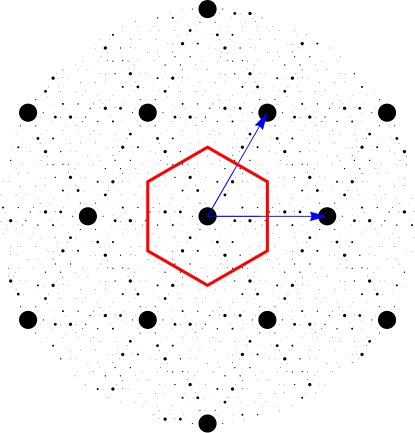
Figure 17. Diffraction image of the aperiodic hexagon tiling. The diffraction measure is lattice periodic, with the lattice of periods given by (4.7). Its generators are indicated by the blue arrows, and a fundamental domain with the red hexagon. The picture shows the intensities of the Bragg peaks in the intersection of the Fourier module with a ball of radius 0.15 in $\mathbb{R}\hskip 0.5pt^{2}$. The intensity of the central peak is the same as for the CASPr tiling. $10$ iterations of the cocycle were used for the computation.

The reprojection of $\mathcal{R}_{{}_{\mathrm{CASPr}}}$ yields a $\mathbb{Z}$-module $\mathcal{R}_{{}_{\mathrm{HT}}}$ of rank $2$, as the HT tiling is again a lattice tiling, this time with return module

$$\mathcal{R}_{{}_{\mathrm{HT}}}\,=\,\frac{\raisebox{-2.0pt}{$1$}}{\raisebox{0.5pt}{$67$}}\bigl{(}-240+84\sqrt{15}-30\hskip 0.5pt\mathrm{i}\sqrt{3}+132\hskip 0.5pt\mathrm{i}\sqrt{5}\,\bigr{)}\mathbb{Z}[\xi]\,=\,\frac{\raisebox{-2.0pt}{$2$}}{\raisebox{0.5pt}{$67$}}\bigl{(}-185-206\xi+20\lambda+44\lambda\xi\bigr{)}\mathbb{Z}[\xi]\hskip 0.5pt.$$

For its dual module, one finds

(4.9) $$\mathcal{R}^{\ast}_{{}_{\mathrm{HT}}}\,=\,\frac{\raisebox{-2.0pt}{$1$}}{\raisebox{0.5pt}{$45$}}\bigl{(}5+2\sqrt{15}-2\hskip 0.5pt\mathrm{i}\sqrt{5}\,\bigr{)}\mathbb{Z}[\xi]\,=\,\frac{\raisebox{-2.0pt}{$1$}}{\raisebox{0.5pt}{$135$}}\bigl{(}-17+16\xi+8\lambda-4\lambda\xi\bigr{)}\mathbb{Z}[\xi]\hskip 0.5pt,$$

which provides the lattice of periods of the diffraction pattern as in the previous case. Note that the length of the period is approximately $3.5$ times larger than in the case of the hexagon tiling. The lattice constant of $\mathcal{R}^{\ast}_{{}_{\mathrm{HT}}}$ reads $\sqrt{\frac{4\lambda+5}{405}}$. Figure 18 shows the intensities of the diffraction measure around the origin.

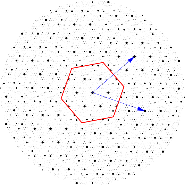
Figure 18. Diffraction image of the Hat–Turtle tiling. The diffraction is lattice periodic, with the lattice of periods given by (4.9), whose generators are indicated by the blue arrows. A fundamental domain is marked by the red hexagon. The picture shows the intensities of the Bragg peaks restricted to the intersection of the Fourier module with a ball of radius 0.5 in $\mathbb{R}\hskip 0.5pt^{2}$. The intensity of the central peak is the same as in the undeformed case. $10$ iterations of the cocycle were used for the computation.

Finally, the Spectre tiling is a further deformation of the HT tiling in the following sense. Hats and Turtles have edges of two different lengths. The Spectre tiling is obtained by rescaling these edges such that their lengths become equal (maintaining the edge directions). Combining the deformation of the HT tiling with this additional deformation results in a relatively simple deformation matrix, one obtains

$$D_{{}_{\mathrm{Sp}}}\,=\,\frac{\raisebox{-2.0pt}{$3-\sqrt{15}$}}{\raisebox{0.5pt}{$6$}}\begin{pmatrix}\sqrt{5}&1\\ 1&-\sqrt{5}\end{pmatrix}.$$

The generators (4.1) are reprojected to the generators $h_{i}$ of the return module of the Spectre tiling and read

$$h_{1} =\,\frac{\raisebox{-2.0pt}{$3$}}{\raisebox{0.5pt}{$2$}}\begin{pmatrix}-1+4\sqrt{3}-3\sqrt{5}\\[1.0pt] 12-3\sqrt{3}-2\sqrt{5}-3\sqrt{15}\end{pmatrix},$$

$$h_{2} =\,\frac{\raisebox{-2.0pt}{$1$}}{\raisebox{0.5pt}{$6$}}\begin{pmatrix}60-98\sqrt{3}+75\sqrt{5}+15\sqrt{15}\,\\[1.0pt] 30+6\sqrt{3}+9\sqrt{5}-7\sqrt{15}\end{pmatrix},$$

$$h_{3} =\,\frac{\raisebox{-2.0pt}{$1$}}{\raisebox{0.5pt}{$2$}}\begin{pmatrix}21-42\sqrt{3}+33\sqrt{5}+6\sqrt{15}\,\\[1.0pt] -6+9\sqrt{3}+6\sqrt{5}+3\sqrt{15}\end{pmatrix},$$

$$h_{4} =\,\frac{\raisebox{-2.0pt}{$3$}}{\raisebox{0.5pt}{$2$}}\begin{pmatrix}-6-3\sqrt{3}+3\sqrt{5}\\[1.0pt] -33+6\sqrt{3}+6\sqrt{5}+9\sqrt{15}\end{pmatrix}.$$

When interpreted as complex numbers, the generators belong to $\mathbb{Q}(\beta)$ with $\beta^{8}-3\beta^{6}+8\beta^{4}-3\beta^{2}+1=0$, a number field containing $\xi,\,\lambda$ and the twelfth root of unity, which is not surprising due to the geometry of the Spectre tiles. We note that the control points of the HT tiling and the Spectre tiling do not differ too much, so the diffraction pattern looks very similar in both cases. The diffraction of the Spectre is shown in Figure 19. We also include a comparison of the diffraction of the HT and Spectre tilings around a point $\tfrac{10}{45}\bigl{(}5+2\sqrt{15},\,-2\sqrt{5}\hskip 0.5pt\bigr{)}^{\top}$ to show the significant difference in both diffraction patterns, see Figure 20.

Figure 19. Diffraction image of the Spectre tiling. The picture shows the intensities of the Bragg peaks restricted to the intersection of the Fourier module with a ball of radius 0.5 in $\mathbb{R}\hskip 0.5pt^{2}$. The intensity of the central peak is the same as in the CASPr tiling. To compute the image, 10 iterations of the cocycle were used.

Figure 20. Diffraction image of the Hat–Turtle (left) and Spectre (right) tiling. Both pictures show the intensities of the Bragg peaks restricted to the intersection of the Fourier module with a ball of radius 0.15 around $\tfrac{10}{45}\bigl{(}5+2\sqrt{15},\,-2\sqrt{5}\hskip 0.5pt\bigr{)}^{\top}$ in $\mathbb{R}\hskip 0.5pt^{2}$. The central point is a lattice point in the lattice of periods of the diffraction measure of HT tiling given by (4.9). $10$ iterations of the cocycle were used for these figures.

We summarise the observations from the last paragraphs in the following theorem.

Theorem 4.2.

The set of control points of the Spectre, Hat–Turtle, and (combinatorial) hexagon tilings are deformed model sets, and can be interpreted as reprojections. They are obtained from the set of control points of the CASPr tiling via the deformation mappings

$$D_{{}_{\mathrm{Sp}}}\, =\,\frac{\raisebox{-2.0pt}{$3-\sqrt{15}$}}{\raisebox{0.5pt}{$6$}}\begin{pmatrix}\sqrt{5}&1\\ 1&-\sqrt{5}\end{pmatrix},$$

$$D_{{}_{\mathrm{HT}}}\, =\,\frac{\raisebox{-2.0pt}{$1$}}{\raisebox{0.5pt}{$201$}}\begin{pmatrix}44\sqrt{15}-231&80\sqrt{3}-84\sqrt{5}\\ 80\sqrt{3}-84\sqrt{5}&231-44\sqrt{15}\end{pmatrix},$$

$$D_{{}_{\mathrm{hex}}}\, =\,\begin{pmatrix}-1&0\\ 0&1\end{pmatrix}.$$

The Fourier module of all these tilings is $L^{\circledast}_{{}_{\mathrm{CASPr}}}$, and for diffraction intensities are

$$I_{\bullet}(k)\,=\,\begin{cases}\bigl{|}H_{{}_{\mathrm{CASPr}}}(k^{\star}-D^{\top}_{\bullet}k)\bigr{|}^{2},&\mbox{if}\ k\in L^{\circledast}_{{}_{\mathrm{CASPr}}},\\ 0,&\mbox{otherwise,}\end{cases}$$

where $\bullet\in\{\mathrm{Sp},\,\mathrm{HT},\,\mathrm{hex}\}$. ∎

Appendix A — $T_{\mathrm{CAP}}$

Here, we give the non-empty matrix blocks for (3.5).

$$T_{12}\,=\,\begin{pmatrix}\bigl{\{}\begin{subarray}{c}{-}\tau{+}1\\ {-}\tau\xi{-}2\xi\end{subarray}\}&\varnothing&\varnothing&\varnothing&\varnothing&\varnothing\\ \varnothing&\bigl{\{}\begin{subarray}{c}\tau{+}2\\ {-}2\tau\xi{-}\xi\end{subarray}\bigr{\}}&\varnothing&\varnothing&\varnothing&\varnothing\\ \varnothing&\varnothing&\bigl{\{}\begin{subarray}{c}2\tau{+}1\\ {-}\tau\xi{+}\xi\end{subarray}\bigr{\}}&\varnothing&\varnothing&\varnothing\\ \varnothing&\varnothing&\varnothing&\bigl{\{}\begin{subarray}{c}\tau{-}1\\ {+}\tau\xi{+}2\xi\end{subarray}\bigr{\}}&\varnothing&\varnothing\\ \varnothing&\varnothing&\varnothing&\varnothing&\bigl{\{}\begin{subarray}{c}{-}\tau{-}2\\ {+}2\tau\xi{+}\xi\end{subarray}\bigr{\}}&\varnothing\\ \varnothing&\varnothing&\varnothing&\varnothing&\varnothing&\bigl{\{}\begin{subarray}{c}{-}2\tau{-}1\\ {+}\tau\xi{-}\xi\end{subarray}\bigr{\}}\\ \end{pmatrix},$$

$$T_{21}\,=\,\begin{pmatrix}\varnothing&\bigl{\{}\begin{subarray}{c}4\tau{+}1\\ +\tau\xi{+}\xi\end{subarray}\bigr{\}}&\varnothing&\varnothing&\varnothing&\varnothing\\ \varnothing&\varnothing&\bigl{\{}\begin{subarray}{c}-\tau{-}1\\ +5\tau\xi{+2\xi}\end{subarray}\bigr{\}}&\varnothing&\varnothing&\varnothing\\ \varnothing&\varnothing&\varnothing&\bigl{\{}\begin{subarray}{c}-5\tau{-}2\\ +4\tau\xi{+}\xi\end{subarray}\bigr{\}}&\varnothing&\varnothing\\ \varnothing&\varnothing&\varnothing&\varnothing&\bigl{\{}\begin{subarray}{c}-4\tau{-}1\\ -\tau\xi{-}\xi\end{subarray}\bigr{\}}&\varnothing\\ \varnothing&\varnothing&\varnothing&\varnothing&\varnothing&\bigl{\{}\begin{subarray}{c}\tau{+}1\\ -5\tau\xi{-}2\xi\end{subarray}\bigr{\}}\\ \bigl{\{}\begin{subarray}{c}5\tau{+}2\\ -4\tau\xi{-}\xi\end{subarray}\bigr{\}}&\varnothing&\varnothing&\varnothing&\varnothing&\varnothing\\ \end{pmatrix},$$

$$T_{22}\,=\,\begin{pmatrix}\bigl{\{}0,\begin{subarray}{c}3\tau+1\\ -3\tau\xi-2\xi\end{subarray}\bigr{\}}&\varnothing&\bigl{\{}\begin{subarray}{c}4\tau{+}1\\ +\tau\xi{+}\xi\end{subarray}\bigr{\}}&\varnothing&\varnothing&\varnothing\\ \varnothing&\bigl{\{}0,\begin{subarray}{c}3\tau+2\\ -\xi\end{subarray}\bigr{\}}&\varnothing&\bigl{\{}\begin{subarray}{c}-\tau{-}1\\ +5\tau\xi{+2\xi}\end{subarray}\bigr{\}}&\varnothing&\varnothing\\ \varnothing&\varnothing&\bigl{\{}0,\begin{subarray}{c}1\\ +3\tau\xi+\xi\end{subarray}\bigr{\}}&\varnothing&\bigl{\{}\begin{subarray}{c}-5\tau{-}2\\ +4\tau\xi{+}\xi\end{subarray}\bigr{\}}&\varnothing\\ \varnothing&\varnothing&\varnothing&\bigl{\{}0,\begin{subarray}{c}-3\tau-1\\ +3\tau\xi+2\xi\end{subarray}\bigr{\}}&\varnothing&\bigl{\{}\begin{subarray}{c}-4\tau{-}1\\ -\tau\xi{-}\xi\end{subarray}\bigr{\}}\\ \bigl{\{}\begin{subarray}{c}\tau{+}1\\ -5\tau\xi{-}2\xi\end{subarray}\bigr{\}}&\varnothing&\varnothing&\varnothing&\bigl{\{}0,\begin{subarray}{c}-3\tau-2\\ +\xi\end{subarray}\bigr{\}}&\varnothing\\ \varnothing&\bigl{\{}\begin{subarray}{c}5\tau{+}2\\ -4\tau\xi{-}\xi\end{subarray}\bigr{\}}&\varnothing&\varnothing&\varnothing&\bigl{\{}0,\begin{subarray}{c}-1\\ -3\tau\xi-\xi\end{subarray}\bigr{\}}\\ \end{pmatrix},$$

$$T_{23}\,=\,\begin{pmatrix}\varnothing&\bigl{\{}\begin{subarray}{c}8\tau+4\\ -4\tau\xi-2\xi\end{subarray}\bigr{\}}&\bigl{\{}\begin{subarray}{c}4\tau+1\\ +\tau\xi+\xi\end{subarray}\bigr{\}}&\varnothing&\varnothing&\varnothing\\ \varnothing&\varnothing&\bigl{\{}\begin{subarray}{c}4\tau+2\\ +4\tau\xi+2\xi\end{subarray}\bigr{\}}&\bigl{\{}\begin{subarray}{c}-\tau-1\\ +5\tau\xi+2\xi\end{subarray}\bigr{\}}&\varnothing&\varnothing\\ \varnothing&\varnothing&\varnothing&\bigl{\{}\begin{subarray}{c}-4\tau-2\\ +8\tau\xi+4\xi\end{subarray}\bigr{\}}&\bigl{\{}\begin{subarray}{c}-5\tau-2\\ +4\tau\xi+\xi\end{subarray}\bigr{\}}&\varnothing\\ \varnothing&\varnothing&\varnothing&\varnothing&\bigl{\{}\begin{subarray}{c}-8\tau-4\\ +4\tau\xi+2\xi\end{subarray}\bigr{\}}&\bigl{\{}\begin{subarray}{c}-4\tau-1\\ -\tau\xi-\xi\end{subarray}\bigr{\}}\\ \bigl{\{}\begin{subarray}{c}\tau+1\\ -5\tau\xi-2\xi\end{subarray}\bigr{\}}&\varnothing&\varnothing&\varnothing&\varnothing&\bigl{\{}\begin{subarray}{c}-4\tau-2\\ -4\tau\xi-2\xi\end{subarray}\bigr{\}}\\ \bigl{\{}\begin{subarray}{c}4\tau+2\\ -8\tau\xi-4\xi\end{subarray}\bigr{\}}&\bigl{\{}\begin{subarray}{c}5\tau+2\\ -4\tau\xi-\xi\end{subarray}\bigr{\}}&\varnothing&\varnothing&\varnothing&\varnothing\\ \end{pmatrix},$$

$$T_{24}\,=\,\begin{pmatrix}\varnothing&\bigl{\{}\begin{subarray}{c}8\tau+4\\ -4\tau\xi-2\xi\end{subarray}\bigr{\}}&\bigl{\{}\begin{subarray}{c}4\tau+1\\ +\tau\xi+\xi\end{subarray}\bigr{\}}&\varnothing&\varnothing&\varnothing\\ \varnothing&\varnothing&\bigl{\{}\begin{subarray}{c}4\tau+2\\ +4\tau\xi+2\xi\end{subarray}\bigr{\}}&\bigl{\{}\begin{subarray}{c}-\tau-1\\ +5\tau\xi+2\xi\end{subarray}\bigr{\}}&\varnothing&\varnothing\\ \varnothing&\varnothing&\varnothing&\bigl{\{}\begin{subarray}{c}-4\tau-2\\ +8\tau\xi+4\xi\end{subarray}\bigr{\}}&\bigl{\{}\begin{subarray}{c}-5\tau-2\\ +4\tau\xi+\xi\end{subarray}\bigr{\}}&\varnothing\\ \varnothing&\varnothing&\varnothing&\varnothing&\bigl{\{}\begin{subarray}{c}-8\tau-4\\ +4\tau\xi+2\xi\end{subarray}\bigr{\}}&\bigl{\{}\begin{subarray}{c}-4\tau-1\\ -\tau\xi-\xi\end{subarray}\bigr{\}}\\ \bigl{\{}\begin{subarray}{c}\tau+1\\ -5\tau\xi-2\xi\end{subarray}\bigr{\}}&\varnothing&\varnothing&\varnothing&\varnothing&\bigl{\{}\begin{subarray}{c}-4\tau-2\\ -4\tau\xi-2\xi\end{subarray}\bigr{\}}\\ \bigl{\{}\begin{subarray}{c}4\tau+2\\ -8\tau\xi-4\xi\end{subarray}\bigr{\}}&\bigl{\{}\begin{subarray}{c}5\tau+2\\ -4\tau\xi-\xi\end{subarray}\bigr{\}}&\varnothing&\varnothing&\varnothing&\varnothing\\ \end{pmatrix},$$

$$T_{32}\,=\,\begin{pmatrix}\varnothing&\varnothing&\varnothing&\bigl{\{}\begin{subarray}{c}-4\tau-3\\ +5\tau\xi+3\xi\end{subarray}\bigr{\}}&\bigl{\{}\begin{subarray}{c}-\tau-1\\ +5\tau\xi+2\xi\end{subarray}\bigr{\}}&\bigl{\{}\begin{subarray}{c}-5\tau-3\\ +\tau\xi\end{subarray}\bigr{\}}\\ \bigl{\{}\begin{subarray}{c}-\tau\\ -4\tau\xi-3\xi\end{subarray}\bigr{\}}&\varnothing&\varnothing&\varnothing&\bigl{\{}\begin{subarray}{c}-5\tau-3\\ +\tau\xi\end{subarray}\bigr{\}}&\bigl{\{}\begin{subarray}{c}-5\tau-2\\ +4\tau\xi+\xi\end{subarray}\bigr{\}}\\ \bigl{\{}\begin{subarray}{c}-4\tau-1\\ -\tau\xi-\xi\end{subarray}\bigr{\}}&\bigl{\{}\begin{subarray}{c}4\tau+3\\ -5\tau\xi-3\xi\end{subarray}\bigr{\}}&\varnothing&\varnothing&\varnothing&\bigl{\{}\begin{subarray}{c}-\tau\\ -4\tau\xi-3\xi\end{subarray}\bigr{\}}\\ \bigl{\{}\begin{subarray}{c}4\tau+3\\ -5\tau\xi-3\xi\end{subarray}\bigr{\}}&\bigl{\{}\begin{subarray}{c}\tau+1\\ -5\tau\xi-2\xi\end{subarray}\bigr{\}}&\bigl{\{}\begin{subarray}{c}5\tau+3\\ -\tau\xi\end{subarray}\bigr{\}}&\varnothing&\varnothing&\varnothing\\ \varnothing&\bigl{\{}\begin{subarray}{c}5\tau+3\\ -\tau\xi\end{subarray}\bigr{\}}&\bigl{\{}\begin{subarray}{c}5\tau+2\\ -4\tau\xi-\xi\end{subarray}\bigr{\}}&\bigl{\{}\begin{subarray}{c}\tau\\ +4\tau\xi+3\xi\end{subarray}\bigr{\}}&\varnothing&\varnothing\\ \varnothing&\varnothing&\bigl{\{}\begin{subarray}{c}\tau\\ +4\tau\xi+3\xi\end{subarray}\bigr{\}}&\bigl{\{}\begin{subarray}{c}4\tau+1\\ +\tau\xi+\xi\end{subarray}\bigr{\}}&\bigl{\{}\begin{subarray}{c}-4\tau-3\\ +5\tau\xi+3\xi\end{subarray}\bigr{\}}&\varnothing\\ \end{pmatrix},$$

$$T_{33}\,=\,T_{34}\,=\,\begin{pmatrix}\varnothing&\varnothing&\varnothing&\varnothing&\varnothing&\bigl{\{}\begin{subarray}{c}-5\tau-3\\ +\tau\xi\end{subarray}\bigr{\}}\\ \bigl{\{}\begin{subarray}{c}-\tau\\ -4\tau\xi-3\xi\end{subarray}\bigr{\}}&\varnothing&\varnothing&\varnothing&\varnothing&\varnothing\\ \varnothing&\bigl{\{}\begin{subarray}{c}4\tau+3\\ -5\tau\xi-3\xi\end{subarray}\bigr{\}}&\varnothing&\varnothing&\varnothing&\varnothing\\ \varnothing&\varnothing&\bigl{\{}\begin{subarray}{c}5\tau+3\\ -\tau\xi\end{subarray}\bigr{\}}&\varnothing&\varnothing&\varnothing\\ \varnothing&\varnothing&\varnothing&\bigl{\{}\begin{subarray}{c}\tau\\ +4\tau\xi+3\xi\end{subarray}\bigr{\}}&\varnothing&\varnothing\\ \varnothing&\varnothing&\varnothing&\varnothing&\bigl{\{}\begin{subarray}{c}-4\tau-3\\ +5\tau\xi+3\xi\end{subarray}\bigr{\}}&\varnothing\\ \end{pmatrix},$$

$$T_{42}\,=\,\begin{pmatrix}\varnothing&\bigl{\{}\begin{subarray}{c}3\tau+1\\ -3\tau\xi-2\xi\end{subarray}\bigr{\}}&\varnothing&\bigl{\{}\begin{subarray}{c}-\tau-2\\ +2\tau\xi+\xi\end{subarray}\bigr{\}}&\varnothing&\bigl{\{}\begin{subarray}{c}-2\tau-2\\ -2\tau\xi-2\xi\end{subarray}\bigr{\}}\\ \bigl{\{}\begin{subarray}{c}2\tau+2\\ -4\tau\xi-4\xi\end{subarray}\bigr{\}}&\varnothing&\bigl{\{}\begin{subarray}{c}3\tau+2\\ -\xi\end{subarray}\bigr{\}}&\varnothing&\bigl{\{}\begin{subarray}{c}-2\tau-1\\ +\tau\xi-\xi\end{subarray}\bigr{\}}&\varnothing\\ \varnothing&\bigl{\{}\begin{subarray}{c}4\tau+4\\ -2\tau\xi-2\xi\end{subarray}\bigr{\}}&\varnothing&\bigl{\{}\begin{subarray}{c}1\\ +3\tau\xi+\xi\end{subarray}\bigr{\}}&\varnothing&\bigl{\{}\begin{subarray}{c}-\tau+1\\ -\tau\xi-2\xi\end{subarray}\bigr{\}}\\ \bigl{\{}\begin{subarray}{c}\tau+2\\ -2\tau\xi-\xi\end{subarray}\bigr{\}}&\varnothing&\bigl{\{}\begin{subarray}{c}2\tau+2\\ +2\tau\xi+2\xi\end{subarray}\bigr{\}}&\varnothing&\bigl{\{}\begin{subarray}{c}-3\tau-1\\ +3\tau\xi+2\xi\end{subarray}\bigr{\}}&\varnothing\\ \varnothing&\bigl{\{}\begin{subarray}{c}2\tau+1\\ -\tau\xi+\xi\end{subarray}\bigr{\}}&\varnothing&\bigl{\{}\begin{subarray}{c}-2\tau-2\\ +4\tau\xi+4\xi\end{subarray}\bigr{\}}&\varnothing&\bigl{\{}\begin{subarray}{c}-3\tau-2\\ +\xi\end{subarray}\bigr{\}}\\ \bigl{\{}\begin{subarray}{c}-1\\ -3\tau\xi-\xi\end{subarray}\bigr{\}}&\varnothing&\bigl{\{}\begin{subarray}{c}\tau-1\\ +\tau\xi+2\xi\end{subarray}\bigr{\}}&\varnothing&\bigl{\{}\begin{subarray}{c}-4\tau-4\\ +2\tau\xi+2\xi\end{subarray}\bigr{\}}&\varnothing\end{pmatrix},$$

$$T_{43}\,=\,\begin{pmatrix}\varnothing&\bigl{\{}\begin{subarray}{c}3\tau+1\\ -3\tau\xi-2\xi\end{subarray}\bigr{\}}&\varnothing&\varnothing&\bigl{\{}\begin{subarray}{c}-9\tau-6\\ +6\tau\xi+3\xi\end{subarray}\bigl{\}}&\varnothing\\ \varnothing&\varnothing&\bigl{\{}\begin{subarray}{c}3\tau+2\\ -\xi\end{subarray}\bigr{\}}&\varnothing&\varnothing&\bigl{\{}\begin{subarray}{c}-6\tau-3\\ -3\tau\xi-3\xi\end{subarray}\bigr{\}}\\ \bigl{\{}\begin{subarray}{c}3\tau+3\\ -9\tau\xi-6\xi\end{subarray}\bigr{\}}&\varnothing&\varnothing&\bigl{\{}\begin{subarray}{c}1\\ +3\tau\xi+\xi\end{subarray}\bigr{\}}&\varnothing&\varnothing\\ \varnothing&\bigl{\{}\begin{subarray}{c}9\tau+6\\ -6\tau\xi-3\xi\end{subarray}\bigl{\}}&\varnothing&\varnothing&\bigl{\{}\begin{subarray}{c}-3\tau-1\\ +3\tau\xi-2\xi\end{subarray}\bigr{\}}&\varnothing&\\ \varnothing&\varnothing&\bigl{\{}\begin{subarray}{c}6\tau+3\\ +3\tau\xi+3\xi\end{subarray}\bigr{\}}&\varnothing&\varnothing&\bigl{\{}\begin{subarray}{c}-3\tau-2\\ +\xi\end{subarray}\bigr{\}}\\ \bigl{\{}\begin{subarray}{c}-1\\ -3\tau\xi-\xi\end{subarray}\bigr{\}}&\varnothing&\varnothing&\bigl{\{}\begin{subarray}{c}-3\tau-3\\ +9\tau\xi+6\xi\end{subarray}\bigr{\}}&\varnothing&\varnothing\end{pmatrix},$$

$$T_{44}\,=\,\begin{pmatrix}\bigl{\{}\begin{subarray}{c}2\tau+1\\ -7\tau\xi-5\xi\end{subarray}\bigr{\}}&\bigl{\{}\begin{subarray}{c}3\tau+1\\ -3\tau\xi-2\xi\end{subarray}\bigr{\}}&\varnothing&\varnothing&\bigl{\{}\begin{subarray}{c}-9\tau-6\\ +6\tau\xi+3\xi\end{subarray}\bigl{\}}&\varnothing\\ \varnothing&\bigl{\{}\begin{subarray}{c}7\tau+5\\ -5\tau\xi-4\xi\end{subarray}\bigr{\}}&\bigl{\{}\begin{subarray}{c}3\tau+2\\ -\xi\end{subarray}\bigr{\}}&\varnothing&\varnothing&\bigl{\{}\begin{subarray}{c}-6\tau-3\\ -3\tau\xi-3\xi\end{subarray}\bigr{\}}\\ \bigl{\{}\begin{subarray}{c}3\tau+3\\ -9\tau\xi-6\xi\end{subarray}\bigr{\}}&\varnothing&\bigl{\{}\begin{subarray}{c}5\tau+4\\ +2\tau\xi+\xi\end{subarray}\bigr{\}}&\bigl{\{}\begin{subarray}{c}1\\ +3\tau\xi+\xi\end{subarray}\bigr{\}}&\varnothing&\varnothing\\ \varnothing&\bigl{\{}\begin{subarray}{c}9\tau+6\\ -6\tau\xi-3\xi\end{subarray}\bigl{\}}&\varnothing&\bigl{\{}\begin{subarray}{c}-2\tau-1\\ +7\tau\xi+5\xi\end{subarray}\bigr{\}}&\bigl{\{}\begin{subarray}{c}-3\tau-1\\ +3\tau\xi-2\xi\end{subarray}\bigr{\}}&\varnothing&\\ \varnothing&\varnothing&\bigl{\{}\begin{subarray}{c}6\tau+3\\ +3\tau\xi+3\xi\end{subarray}\bigr{\}}&\varnothing&\bigl{\{}\begin{subarray}{c}-7\tau-5\\ +5\tau\xi+4\xi\end{subarray}\bigr{\}}&\bigl{\{}\begin{subarray}{c}-3\tau-2\\ +\xi\end{subarray}\bigr{\}}\\ \bigl{\{}\begin{subarray}{c}-1\\ -3\tau\xi-\xi\end{subarray}\bigr{\}}&\varnothing&\varnothing&\bigl{\{}\begin{subarray}{c}-3\tau-3\\ +9\tau\xi+6\xi\end{subarray}\bigr{\}}&\varnothing&\bigl{\{}\begin{subarray}{c}-5\tau-4\\ -2\tau\xi-\xi\end{subarray}\bigr{\}}\end{pmatrix}.$$

References

- [1] M. Baake, F. Gähler and P. Gohlke, Orbit separation dimension as complexity measure for primitive inflation tilings, preprint; arXiv:2311.03541.
- [2] M. Baake, F. Gähler, J. Mazáč and L. Sadun, On the long-range order of the Spectre tilings, preprint; arXiv:2411.15503.
- [3] M. Baake, F. Gähler and L. Sadun, Dynamics and topology of the Hat family of tilings, preprint; arXiv:2305.05639.
- [4] M. Baake, A. Gorodetski and J. Mazáč, A naturally appearing family of Cantorvals, Lett. Math. Phys. 114 (2024) 101:1–11; arXiv:2401.05372.
- [5] M. Baake and U. Grimm, Aperiodic Order. Vol. 1: A Mathematical Invitation, Cambridge University Press, Cambridge (2013).
- [6] M. Baake and U. Grimm, Fourier transform of Rauzy fractals and point spectrum of 1D Pisot inflation tilings, Docum. Math. 25 (2020) 2303–2337; arXiv:1907.11012.
- [7] M. Baake and U. Grimm, Diffraction of a model set with complex windows, J. Phys.: Conf. Ser. 1458 (2020) 012006:1-6; arXiv:1904.08285.
- [8] M. Baake and A. Haynes, Convergence of Fourier–Bohr coefficients for regular Euclidean model sets, preprint; arXiv:2308.07105.
- [9] M. Baake and D. Lenz, Dynamical systems on translation bounded measures: Pure point dynamical and diffraction spectra, Ergod. Th. Dynam. Syst. 24 (2004) 1867–1893; arXiv:math.DS/0302061.
- [10] M. Baake and D. Lenz, Deformation of Delone dynamical systems and pure point diffraction, J. Fourier Anal. Appl. 11 (2005) 125–150; arXiv:math.DS/0404155.
- [11] G. Bernuau and M. Dunau, Fourier analysis of deformed model sets, in Directions in Mathematical Quasicrystals, eds. M. Baake and R.V. Moody, Fields Institute Monographs, vol. 13, Amer. Math. Society, Providence, RI (2000), pp. 43–60.
- [12] V. Berthé, H. Ei, S. Ito and H. Rao, On substitution invariant Sturmian words: An application of Rauzy fractals, RAIRO – Theor. Inform. Appl. 41 (2007) 329–349.
-
[13]
A. Clark and L. Sadun,
When size matters,
Ergod. Th. Dynam. Syst. 23 (2003) 1043–1057;
arXiv:math.DS/0201152. -
[14]
A. Clark and L. Sadun,
When shape matters,
Ergod. Th. Dynam. Syst. 26 (2006) 69–86;
arXiv:math.DS/0306214. - [15] D.-J. Feng, M. Furukado, S. Ito and J. Wu, Pisot substitutions and Hausdorff dimension of boundaries of atomic surfaces, Tsukuba J. Math. 30 (2006) 195–223.
- [16] J.E. Hutchinson, Fractals and self-similarity, Indiana Univ. Math. J. 30 (1981) 713–747.
- [17] J. Kellendonk and L. Sadun, Conjugacies of Model Sets, Discr. Cont. Dynam. Syst. A 37 (2017) 3805–3830; arxiv:1406.3851.
- [18] The LMFDB Collaboration, The L-functions and modular forms database, https://www.lmfdb.org (2024).
- [19] D. Lenz, Continuity of eigenfunctions of uniquely ergodic dynamical systems and intensity of Bragg peaks, Commun. Math. Phys. 287 (2009) 225–258; arXiv:math-ph/0608026.
- [20] D. Lenz, T. Spindeler and N. Strungaru, Pure Point Diffraction and mean, Besicovitch and Weyl almost periodicity, Ergod. Th. Dynam. Syst. 44 (2024) 524–568; arXiv:2006.10821.
- [21] J.M. Luck, C. Godrèche, A. Janner and T. Janssen, The nature of the atomic surfaces of quasiperiodic self-similar structures, J. Phys. A: Math. Gen. 26 (1993) 1951–1999.
- [22] R.D. Mauldin amd S.C. Williams, Hausdorff dimension in graph directed constructions, Trans. Amer. Math. Soc. 309 (1988) 811–829.
- [23] J. Mazáč, Fractal and Statistical Phenomena in Aperiodic Order, PhD thesis, Bielefeld University, in preparation.
- [24] Y. Meyer, Algebraic Numbers and Harmonic Analysis, North Holland, Amsterdam (1972).
- [25] R.V. Moody, Meyer sets and their duals, in The Mathematics of Long-Range Aperiodic Order, ed. R. V. Moody, NATO ASI Series C 489, Kluwer, Dordrecht (1997), pp. 403–441.
- [26] R.V. Moody, Uniform distribution in model sets, Can. Math. Bull. 45 (2002) 123–130.
- [27] N. Pytheas Fogg, Substitutions in Dynamics, Arithmetics and Combinatorics, eds. V. Berthé, S. Ferenczi, C. Mauduit and A. Siegel, LNM 1794, Springer, Berlin (2002).
- [28] M. Schlottmann, Cut-and-project sets in locally compact Abelian groups, in Quasicrystals and Discrete Geometry, ed. J. Patera, Fields Institute Monographs, vol. 10, Amer. Math. Society, Providence, RI (1998), pp. 247–264.
- [29] A. Siegel and J. Thuswaldner, Topological properties of Rauzy fractals, Mémoires SMF 118 (2009).
- [30] B. Sing, Pisot Substitutions and Beyond, PhD thesis (Bielefeld University, 2007); available electronically at urn:nbn:de:hbz:361-11555.
- [31] D. Smith, J.S. Myers, C.S. Kaplan and C. Goodman-Strauss, An aperiodic monotile, Combin. Th. 4 (2024) 6:1–91; arXiv:2303.10798.
- [32] D. Smith, J.S. Myers, C.S. Kaplan and C. Goodman-Strauss, A chiral aperiodic monotile, Combin. Th. 4 (2024) 13:1–25; arXiv:2305.17743.
- [33] J.E.S. Socolar, Quasicrystalline structure of the hat monotile tilings, Phys. Rev. B 108 (2023) 224109:1–12; arXiv:2305.01174.
- [34] K.R. Wicks, Fractals and Hyperspaces, LNM 1492, Springer, Berlin (1991).