On Lebesgue points and measurability with Choquet integrals

Petteri Harjulehto Department of Mathematics and Statistics, FI-00014 University of Helsinki, Finland petteri.harjulehto@helsinki.fi  and  Ritva Hurri-Syrjänen Department of Mathematics and Statistics, FI-00014 University of Helsinki, Finland ritva.hurri-syrjanen@helsinki.fi
(Date: March 5, 2025)
Abstract.

We consider Choquet integrals with respect to dyadic Hausdorff content of non-negative functions which are not necessarily Lebesgue measurable. We study the theory of Lebesgue points. The studies yield convergence results and also a density result between function spaces. We provide examples which show sharpness of the main convergence theorem. These examples give additional information about the convergence in the norm also, namely the difference of the functions in this setting and continuous functions.

Key words and phrases:
Choquet integral, dyadic Hausdorff content, dyadic Hausdorff capacity, Lebesgue point, maximal operator, non-measurable function
2020 Mathematics Subject Classification:
28A25, 28A20, 42B25

1. Introduction

The Choquet integral was introduced by G. Choquet [11] and applied by D. R. Adams in the study of nonlinear potential theory [2, 3, 4]. Later on, J. Xiao has studied Choquet integrals extensively with Adams [5] and with his other coauthors [12, 38]. Recently, there has arisen a new interest in Choquet integrals and their properties. We refer to [39, 32, 28, 29, 9, 10, 17, 18, 33, 19, 20, 24, 21, 7].

Choquet integral theory has been concentrated to the context when functions are continuous or quasicontinuous or at least Lebesgue measurable. However, this seems not to be necessary. As in the case of the Riemann and Lebesgue integral theories which were developed for Lebesgue measurable functions first, and later on, these integral theories emerged when functions are not Lebesgue measurable [23, 25, 43], also now it seems that it is worth to study properties of Choquet integrals for functions which are not necessarily Lebesgue measurable. Recall that D. Denneberg does the ground work in his monograph [13] where he has stated and proved properties of Choquet integrals with respect to capacities with minimal assumptions on these capacities as well as functions.

We are interested in Choquet integrals with respect to dyadic Hausdorff content, that is dyadic Hausdorff capacity. We study Lebesgue point properties using Choquet integrals with respect to dyadic Hausdorff content. We pay special attention to the assumption of Lebesgue measurability. As a by-product of results we obtain a characterization for Lebesgue measurable functions:

1.1 Corollary.

Let $n\geq 1$. Suppose that $f:{\varmathbb{R}^{n}}\to[0,\infty]$ is a function such that $\int_{B}f(y)\,d\tilde{\mathcal{H}}^{n}_{\infty}(y)<\infty$ for all open balls $B$ in ${\varmathbb{R}^{n}}$. Then, the function $f$ is Lebesgue measurable if and only if

$$f(x)=\limsup_{r\to 0^{+}}\frac{1}{\tilde{\mathcal{H}}^{n}_{\infty}(B(x,r))}\int_{B(x,r)}f(y)\,d\tilde{\mathcal{H}}^{n}_{\infty}(y)$$

for $\tilde{\mathcal{H}}^{n}_{\infty}$-almost every $x\in{\varmathbb{R}^{n}}$.

In Section 2 and Section 3 we recall definitions and basic properties for dyadic Hausdorff content and Choquet integral with respect to dyadic Hausdorf content, respectively. We start Section 4 by proving convergence results for increasing sequences of non-negative functions when integrals are taken in Choquet sense with respect to dyadic Hausdorff content. Later on, we recall the definitions needed for study Hausdorff content maximal functions and the function space ${\textsc{n}L}^{1}(\Omega,\tilde{\mathcal{H}}^{\delta}_{\infty})$, $0<\delta\leq n$. In Section 5 we concentrate on properties related to Lebesgue points in this context and introduce the concept of ${\textsc{n}L}^{1}$-limit of continuous functions in Definition 5.8 for non-negative functions in the space ${\textsc{n}L}^{1}(\Omega,\tilde{\mathcal{H}}^{\delta}_{\infty})$, $0<\delta\leq n$. This will lead us study functions defined in this space and denseness of continuous functions there. In Section 6 we provide two examples of Lebesgue measurable functions from ${\textsc{n}L}^{1}(\Omega,\tilde{\mathcal{H}}^{\delta}_{\infty})$, $0<\delta<n$, which are not ${\textsc{n}L}^{1}$-limits of continuos functions. In particular, these examples show that continuous functions are not dense in the space ${\textsc{n}L}^{1}({\varmathbb{R}^{n}},\tilde{\mathcal{H}}^{\delta}_{\infty})$ if $0<\delta<n$, Remark 6.3. The examples also show necessity and sharpness of our assumption in one of our main theorems, Theorem 5.9.

2. Hausdorff content

We recall the definition of the $\delta$-dimensional dyadic Hausdorff content for any given set in ${\varmathbb{R}^{n}}$, [42]. Cubes in ${\varmathbb{R}^{n}}$ are denoted by $Q$ and the side length of a given cube $Q$ is written as $\ell(Q)$.

We let $E$ be a set in ${\varmathbb{R}^{n}}$, $n\geq 1$, and suppose that $\delta\in(0,n]$. The $\delta$-dimensional dyadic Hausdorff content for any given set $E$ in ${\varmathbb{R}^{n}}$ is defined by

$$\tilde{\mathcal{H}}_{\infty}^{\delta}(E):=\inf\bigg{\{}\sum_{i=1}^{\infty}\ell(Q_{i})^{\delta}:E\subset\mathop{int}\nolimits\big{(}\bigcup_{i=1}^{\infty}Q_{i}\big{)}\bigg{\}}\,,$$

where the infimum is taken over all countably (or finite) collections of dyadic cubes such that the interior of the union of the cubes covers $E$. If $k\in\varmathbb{Z}$ is fixed, we write $\mathcal{Q}_{k}$ for a collection of cubes whose vertices are from the lattice $(2^{k}\varmathbb{Z})^{n}$. This means that the side length of cubes is $2^{k}$ and each cube is congruent to a cube $[0,2^{k})^{n}$. It is customary to call these cubes half open. By dyadic cubes we mean an union of collection of cubes $\bigcup_{k\in\varmathbb{Z}}\mathcal{Q}_{k}$.

The cube covering is called a dyadic cube covering or dyadic cube cover.

The $\delta$-dimensional dyadic Hausdorff content $\tilde{\mathcal{H}}_{\infty}^{\delta}$ satisfies the following useful properties, which means that it is a Choquet capacity.

  1. (H1)

    $\tilde{\mathcal{H}}_{\infty}^{\delta}(\emptyset)=0$;

  2. (H2)

    (monotonicity) if $A\subset B$, then $\tilde{\mathcal{H}}_{\infty}^{\delta}(A)\leq\tilde{\mathcal{H}}_{\infty}^{\delta}(B)$;

  3. (H3)

    (subadditivity) if $(A_{i})$ is any sequence of sets, then

    $$\tilde{\mathcal{H}}_{\infty}^{\delta}\Big{(}\bigcup_{i=1}^{\infty}A_{i}\Big{)}\leq\sum_{i=1}^{\infty}\tilde{\mathcal{H}}_{\infty}^{\delta}(A_{i});$$
  4. (H4)

    if $(K_{i})$ is a decreasing sequence of compact sets, then

    $$\tilde{\mathcal{H}}_{\infty}^{\delta}\Big{(}\bigcap_{i=1}^{\infty}K_{i}\Big{)}=\lim_{i\to\infty}\tilde{\mathcal{H}}_{\infty}^{\delta}(K_{i});$$
  5. (H5)

    if $(E_{i})$ is an increasing sequence of sets, then

    $$\tilde{\mathcal{H}}_{\infty}^{\delta}\big{(}\bigcup_{i=1}^{\infty}E_{i}\big{)}=\lim_{i\to\infty}\tilde{\mathcal{H}}_{\infty}^{\delta}(E_{i}).$$

Moreover, $\tilde{\mathcal{H}}_{\infty}^{\delta}$ is strongly subadditive, that is

(2.1) $$\tilde{\mathcal{H}}_{\infty}^{\delta}(A_{1}\cup A_{2})+\tilde{\mathcal{H}}_{\infty}^{\delta}(A_{1}\cap A_{2})\leq\tilde{\mathcal{H}}_{\infty}^{\delta}(A_{1})+\tilde{\mathcal{H}}_{\infty}^{\delta}(A_{2})$$

for all subsets $A_{1},A_{2}$ in ${\varmathbb{R}^{n}}$.

For the validity of these properties we refer to [42, Theorem 2.1, Propositions 2.3 and 2.4]. We point out that property (2.1) is called submodularity by D. Denneberg [13, p. 16].

3. Choquet integral

We recall the definition of Choquet integral, now with respect to the dyadic Hausdorff content. Let $\Omega$ be a subset of ${\varmathbb{R}^{n}}$, $n\geq 1$. For any function $f:\Omega\to[0,\infty]$ the integral in the sense of Choquet with respect to the $\delta$-dimensional dyadic Hausdorff content is defined by

(3.1) $$\int_{\Omega}f(x)\,d\tilde{\mathcal{H}}^{\delta}_{\infty}:=\int_{0}^{\infty}\tilde{\mathcal{H}}^{\delta}_{\infty}\big{(}\{x\in\Omega:f(x)>t\}\big{)}\,dt.$$

Since $\tilde{\mathcal{H}}_{\infty}^{\delta}$ is a monotone set function, the corresponding distribution function $t\mapsto\tilde{\mathcal{H}}^{\delta}_{\infty}\big{(}\{x\in\Omega:f(x)>t\}\big{)}$ for any function $f:\Omega\to[0,\infty]$ is decreasing with respect to $t$. By decreasing property the distribution function $t\mapsto\tilde{\mathcal{H}}^{\delta}_{\infty}\big{(}\{x\in\Omega:f(x)>t\}\big{)}$ is measurable with respect to the 1-dimensional Lebesgue measure. Thus, $\int_{0}^{\infty}\tilde{\mathcal{H}}^{\delta}_{\infty}\big{(}\{x\in\Omega:f(x)>t\}\big{)}\,dt$ is well defined as a Lebesgue integral. The right-hand side of (3.1) can be understood also as an improper Riemann integral, since a decreasing function is Riemann integrable. The wording any function in the present paper means that the only requirement is that the function is well defined. We emphasise that the Choquet integral is well defined for any non-measurable set in ${\varmathbb{R}^{n}}$ and for any non-measurable function. A classical example of a non-measurable function is a characteristic function of a non-measurable set, originally constructed by G. Vitali [40].

We use the following properties of the Choquet integral with respect to the dyadic Hausdorff content frequently. For these basic properties and others we refer to [3], [4, Chapter 4], [8], and [21].

3.2 Lemma.

Suppose that $\Omega$ is a subset of ${\varmathbb{R}^{n}}$, functions $f,g:\Omega\to[0,\infty]$ are non-negative, and $\delta\in(0,n]$. Then:

  1. (I1)

    $\displaystyle\int_{\Omega}af(x)\,d\tilde{\mathcal{H}}_{\infty}^{\delta}=a\int_{\Omega}f(x)\,d\tilde{\mathcal{H}}_{\infty}^{\delta}$ with any $a\geq 0$;

  2. (I2)

    $\displaystyle\int_{\Omega}f(x)\,d\tilde{\mathcal{H}}_{\infty}^{\delta}=0$ if and only if $f(x)=0$ for $\tilde{\mathcal{H}}_{\infty}^{\delta}$-almost every $x\in\Omega$;

  3. (I3)

    if $E\subset{\varmathbb{R}^{n}}$, then $\displaystyle\int_{\Omega}\chi_{E}(x)\,d\tilde{\mathcal{H}}_{\infty}^{\delta}=\tilde{\mathcal{H}}_{\infty}^{\delta}(\Omega\cap E)$;

  4. (I4)

    if $A\subset B\subset\Omega$, then $\int_{A}f(x)\,d\tilde{\mathcal{H}}_{\infty}^{\delta}\leq\int_{B}f(x)\,d\tilde{\mathcal{H}}_{\infty}^{\delta}$;

  5. (I5)

    if $0\leq f\leq g$, then $\displaystyle\int_{\Omega}f(x)\,d\tilde{\mathcal{H}}_{\infty}^{\delta}\leq\int_{\Omega}g(x)\,d\tilde{\mathcal{H}}_{\infty}^{\delta}$.

3.3 Remark.

Note that if $\Omega\subset{\varmathbb{R}^{n}}$ is a Lebesgue measurable set, then by [21, Remark 3.4] there exists a constant $c(n)>0$ such that

(3.4) $$\frac{1}{c(n)}\int_{\Omega}|f(x)|\,d\tilde{\mathcal{H}}^{n}_{\infty}\leq\int_{\Omega}|f(x)|\,dx\leq c(n)\int_{\Omega}|f(x)|\,d\tilde{\mathcal{H}}^{n}_{\infty}$$

for all Lebesgue measurable functions $f:\Omega\to[-\infty,\infty]$.

Recall that a Choquet integral with respect to a set function $H:\mathcal{P}({\varmathbb{R}^{n}})\to[0,\infty]$ is sublinear, if the inequality

$$\int_{\Omega}\sum_{i=1}^{\infty}f_{i}(x)dH\leq K\sum_{i=1}^{\infty}\int_{\Omega}f_{i}(x)dH$$

holds with $K=1$ for all sequences $(f_{i})$ of functions $f_{i}:\Omega\to[0,\infty]$. By [13, Chapter 6], a necessary condition for the Choquet integral to be sublinear is that the corresponding set function $H$ is strongly subadditive, that is

$$H(A_{1}\cup A_{2})+H(A_{1}\cap A_{2})\leq H(A_{1})+H(A_{2})$$

for all subsets $A_{1}$ and $A_{2}$ in ${\varmathbb{R}^{n}}$. Since the dyadic Hausdorff content $\tilde{\mathcal{H}}_{\infty}^{\delta}$ is a monotone and strongly subadditive set function by (H2) and (2.1) and we use only non-negative functions, Denneberg’s result [13, Theorem 6.3, p. 75] shows that Choquet integral with respect to the dyadic Hausdorff content $\tilde{\mathcal{H}}_{\infty}^{\delta}$ is sublinear.

3.5 Theorem.

[13, Theorem 6.3]. If $\Omega$ is a subset of ${\varmathbb{R}^{n}}$ and $\delta\in(0,n]$, then for all sequences $(f_{i})$ of non-negative functions $f_{i}:\Omega\to[0,\infty]$

$$\int_{\Omega}\sum_{i=1}^{\infty}f_{i}(x)d\tilde{\mathcal{H}}_{\infty}^{\delta}\leq\sum_{i=1}^{\infty}\int_{\Omega}f_{i}(x)d\tilde{\mathcal{H}}_{\infty}^{\delta}.$$

We point out that Denneberg stated and proved his theorem [13, Theorem 6.3] for a more general setting.

4. Auxiliary convergence results

We prove a monotone convergence result and Fatou’s lemma for non-negative functions in this setting. For a similar convergence theorem we refer to [13, Theorem 8.1] where the situation is more general. On the other hand, convergence results with different additional assumptions than ours have been proved in [26] and [33], for example.

4.1 Proposition.

Suppose that $\delta\in(0,n]$. If $(f_{i})$ is a sequence of non-negative increasing functions $f_{i}:\Omega\to[0,\infty]$ and $f(x)=\lim_{i\to\infty}f_{i}(x)$ for every $x\in\Omega$, then

$$\lim_{i\to\infty}\int_{\Omega}f_{i}\,d\tilde{\mathcal{H}}_{\infty}^{\delta}=\int_{\Omega}f\,d\tilde{\mathcal{H}}_{\infty}^{\delta}.$$
Proof.

Since the sequence $(f_{i})$ is increasing, the monotonicity property (H2) of the set function $\tilde{\mathcal{H}}_{\infty}^{\delta}$ yields that

$$\tilde{\mathcal{H}}_{\infty}^{\delta}\big{(}\{x\in\Omega:f_{i}(x)>t\}\big{)}\leq\tilde{\mathcal{H}}_{\infty}^{\delta}\big{(}\{x\in\Omega:f_{i+1}(x)>t\}\big{)}\mbox{ for all }t\geq 0\,.$$

This means that the set function $t\mapsto\tilde{\mathcal{H}}_{\infty}^{\delta}\big{(}\{x\in\Omega:f_{i}(x)>t\}\big{)}$ is increasing with respect to the index $i$. Hence, the Lebesgue monotone convergence results in $\varmathbb{R}$, for example [15, 2.14], imply that

$$\begin{split}\lim_{i\to\infty}\int_{\Omega}f_{i}\,d\tilde{\mathcal{H}}_{\infty}^{\delta}&=\lim_{i\to\infty}\int_{0}^{\infty}\tilde{\mathcal{H}}_{\infty}^{\delta}\big{(}\{x\in\Omega:f_{i}(x)>t\}\big{)}\,dt\\ &=\int_{0}^{\infty}\lim_{i\to\infty}\tilde{\mathcal{H}}_{\infty}^{\delta}\big{(}\{x\in\Omega:f_{i}(x)>t\}\big{)}\,dt\,.\end{split}$$

By property (H5) we obtain the claim. Namely,

$\displaystyle\int_{0}^{\infty}\lim_{i\to\infty}\tilde{\mathcal{H}}_{\infty}^{\delta}\big{(}\{x\in\Omega:f_{i}(x)>t\}\big{)}\,dt=\int_{0}^{\infty}\tilde{\mathcal{H}}_{\infty}^{\delta}\Big{(}\bigcup_{i=1}^{\infty}\{x\in\Omega:f_{i}(x)>t\}\Big{)}\,dt$
$\displaystyle\quad=\int_{0}^{\infty}\tilde{\mathcal{H}}_{\infty}^{\delta}\big{(}\{x\in\Omega:f(x)>t\}\big{)}\,dt=\int_{\Omega}f\,d\tilde{\mathcal{H}}_{\infty}^{\delta}.\qed$

The previous convergence result gives Fatou’s lemma.

4.2 Proposition.

Let $\delta\in(0,n]$. If $(f_{i})$ is a sequence of non-negative functions defined on $\Omega$, then

$$\int_{\Omega}\liminf_{i\to\infty}f_{i}\,d\tilde{\mathcal{H}}_{\infty}^{\delta} \leq\liminf_{i\to\infty}\int_{\Omega}f_{i}\,d\tilde{\mathcal{H}}_{\infty}^{\delta}\,.$$
Proof.

Let us write that $g_{k}(x):=\inf_{j\geq k}f_{j}(x)$. Then $(g_{k})$ is an increasing sequence and $\lim_{k\to\infty}g_{k}(x)=\liminf_{i\to\infty}f_{i}(x)$. By Proposition 4.1 we obtain

$$\begin{split}\int_{\Omega}\liminf_{i\to\infty}f_{i}\,d\tilde{\mathcal{H}}_{\infty}^{\delta}&=\int_{\Omega}\lim_{k\to\infty}g_{k}\,d\tilde{\mathcal{H}}_{\infty}^{\delta}=\lim_{k\to\infty}\int_{\Omega}g_{k}\,d\tilde{\mathcal{H}}_{\infty}^{\delta}\leq\liminf_{k\to\infty}\int_{\Omega}f_{k}\,d\tilde{\mathcal{H}}_{\infty}^{\delta}.\end{split}$$

We recall a definition of a space of functions which are not necessarily Lebesgue measurable, [21, Remark 3.11] .

4.3 Definition.

Let $\Omega$ be a subset of ${\varmathbb{R}^{n}}$, $n\geq 1$, and $0<\delta\leq n$. We write

$${\textsc{n}L}^{1}(\Omega,\tilde{\mathcal{H}}^{\delta}_{\infty}):=\Big{\{}f:\Omega\to[-\infty,\infty]:\int_{\Omega}|f|d\mathcal{H}^{\delta}_{\infty}<\infty\Big{\}}.$$

Here, by a function we mean an equivalent class of functions that coincide $\tilde{\mathcal{H}}^{\delta}_{\infty}$-almost everywhere. Property (I1) and Theorem 3.5 imply that ${\textsc{n}L}^{1}(\Omega,\mathcal{H}^{\delta}_{\infty})$ is an $\varmathbb{R}$-vector space. We denote

(4.4) $$\|f\|_{1}:=\int_{\varmathbb{R}^{n}}|f|\,d\tilde{\mathcal{H}}^{\delta}_{\infty}.$$

Theorem 3.5 together (I1) yields the following proposition.

4.5 Proposition.

The notion $\|\cdot\|_{1}$ is a norm in ${\textsc{n}L}^{1}(\Omega,\tilde{\mathcal{H}}^{\delta}_{\infty})$.

More information about ${\textsc{n}L}^{1}(\Omega,\mathcal{H}^{\delta}_{\infty})$-spaces can be found in [21, Chapter 3]. By $f\in{\textsc{n}L}^{1}_{\mathop{loc}\nolimits}({\varmathbb{R}^{n}},\tilde{\mathcal{H}}^{\delta}_{\infty})$ we mean that $f\in{\textsc{n}L}^{1}(K,\tilde{\mathcal{H}}^{\delta}_{\infty})$ whenever $K\subset{\varmathbb{R}^{n}}$ is a bounded set.

4.6 Theorem.

Let $\delta\in(0,n]$ and $f\in{\textsc{n}L}^{1}({\varmathbb{R}^{n}},\tilde{\mathcal{H}}^{\delta}_{\infty})$. If $(f_{i})$ is a sequence of ${\textsc{n}L}^{1}({\varmathbb{R}^{n}},\tilde{\mathcal{H}}^{\delta}_{\infty})$-functions such that $\lim_{i\to\infty}\|f-f_{i}\|_{1}=0$, then there exists a subsequence $(f_{i_{j}})$ which converges to $f$ pointwise for $\tilde{\mathcal{H}}^{\delta}_{\infty}$-almost every $x\in{\varmathbb{R}^{n}}$.

Proof.

Since $\|f_{i}-f_{j}\|_{1}\leq\|f_{i}-f\|_{1}+\|f_{j}-f\|_{1}$ by Proposition 4.5, the standard argument yields that $(f_{i})$ is a Cauchy sequence with respect to  $\|\cdot\|_{1}$. Let us choose a suitable subsequence of $(f_{i})$. Choose $i_{1}$ so that $\|f_{i}-f_{j}\|<\tfrac{1}{2}$ when $i,j\geq i_{1}$. Assume that $i_{1},\ldots\,,i_{m}$ have be chosen so that $\|f_{i}-f_{j}\|<\tfrac{1}{2^{m}}$ when $i,j\geq i_{m}$. Then we choose $i_{m+1}$ so that $\|f_{i}-f_{j}\|<\tfrac{1}{2^{m+1}}$ when $i,j\geq i_{m+1}$ and $i_{m+1}>i_{m}$. For the subsequence $(f_{i_{j}})$ we have

$$\|f_{i_{j+1}}-f_{i_{j}}\|_{1}<\frac{1}{2^{i_{j}}}.$$

Let us write

$$g_{m}(x):=\sum_{j=1}^{m}|f_{i_{j}}(x)-f_{i_{j+1}}(x)|\quad\text{and}\quad g(x):=\sum_{j=1}^{\infty}|f_{i_{j}}(x)-f_{i_{j+1}}(x)|.$$

Since $(g_{m})$ is a pointwise increasing sequence, Proposition 4.1 and Theorem 3.5 imply that

$$\begin{split}\|g\|_{1}&=\|\lim_{m\to\infty}g_{m}\|_{1}=\lim_{m\to\infty}\|g_{m}\|_{1}=\lim_{m\to\infty}\int_{\varmathbb{R}^{n}}\sum_{j=1}^{m}|f_{i_{j}}(x)-f_{i_{j+1}}(x)|\,d\tilde{\mathcal{H}}^{\delta}_{\infty}(x)\\ &\leq\lim_{m\to\infty}\sum_{j=1}^{m}\int_{\varmathbb{R}^{n}}|f_{i_{j}}(x)-f_{i_{j+1}}(x)|\,d\tilde{\mathcal{H}}^{\delta}_{\infty}(x)\leq\sum_{j=1}^{\infty}\frac{1}{2^{i_{j}}}\leq 1.\end{split}$$

This means that $g$ is finite $\tilde{\mathcal{H}}^{\delta}_{\infty}$-almost everywhere. Let us study the telescopic series $f_{i_{1}}(x)+\sum_{k=1}^{\infty}(f_{i_{k}}(x)-f_{i_{k+1}}(x))$. In the points where $g(x)<\infty$, the telescopic series converges absolutely, and thus the telescopic series also converges $\tilde{\mathcal{H}}^{\delta}_{\infty}$-almost everywhere. Let us denote by $h(x)$ the limit in the points where the telescopic series converges, let $h(x)=0$ otherwise. Then we have

$$\begin{split}h(x)&=f_{i_{1}}(x)+\sum_{j=1}^{\infty}(f_{i_{j}}(x)-f_{i_{j+1}}(x))=\lim_{m\to\infty}\Big{(}f_{i_{1}}(x)+\sum_{j=1}^{m-1}(f_{i_{j}}(x)-f_{i_{j+1}}(x))\Big{)}\\ &=\lim_{m\to\infty}f_{i_{m}}(x)\end{split}$$

on the points where the telescopic series converges.

Let us then show that $\lim_{i \to\infty}\|h-f_{i}\|_{1}=0$. Let $\varepsilon>0$. Since $(f_{i})$ is a Cauchy-sequence there exists $i_{\varepsilon}$ such that $\|f_{i}-f_{j}\|_{1}<\varepsilon$ when $i,j\geq i_{\varepsilon}$. For a fixed $i$ we have $f_{i_{j}}(x)-f_{i}(x)\to h(x)-f_{i}(x)$ as $j\to\infty$ for $\tilde{\mathcal{H}}^{\delta}_{\infty}$-almost every $x\in{\varmathbb{R}^{n}}$. Proposition 4.2 implies that

$$\begin{split}\|h-f_{i}\|_{1}=\|\lim_{j\to\infty}|f_{i_{j}}-f_{i}|\|_{1}\leq\liminf_{j\to\infty}\|f_{i_{j}}-f_{i}\|\leq\varepsilon\end{split}$$

when $i\geq i_{\varepsilon}$.

Finally, the assumption $\lim_{i\to\infty}\|f-f_{i}\|_{1}=0$ and the previous step yield that

$$\|f-h\|_{1}\leq\|f-f_{i}\|_{1}+\|f_{i}-h\|_{1}\to 0\mbox{ as }i \to\infty\,.$$

Hence, $f(x)=h(x)$ for $\tilde{\mathcal{H}}^{\delta}_{\infty}$-almost every $x\in{\varmathbb{R}^{n}}$. ∎

Let $\delta\in(0,n]$. We recall that the Hausdorff content centred maximal function is defined as

(4.7) $$\mathcal{M}^{\delta}f(x):=\sup_{r>0}\frac{1}{\tilde{\mathcal{H}}_{\infty}^{\delta}(B(x,r))}\int_{B(x,r)}|f|\,d\tilde{\mathcal{H}}_{\infty}^{\delta}\,,$$

[9], [21, (4.1)].

We need the following result, which comes from [7, Theorem A] by choosing $\varphi(t)=t^{\delta}$ and noting that the different Hausdorff contents are comparable [42, Proposition 2.3]. This maximal function for non-measurable functions in the case $\delta=n$ have been studied also in [21], where strong-type estimates have been proved.

4.8 Theorem.

[7, Theorem A] Let $\delta\in(0,n]$. Then there exists a constant $c$ depending only on $\delta$ and $n$ such that

(4.9) $$\tilde{\mathcal{H}}^{\delta}_{\infty}\Big{(}\{x\in{\varmathbb{R}^{n}}:\mathcal{M}^{\delta}f(x)>t\}\Big{)}\leq\frac{c}{t}\int_{\varmathbb{R}^{n}}|f|\,d\tilde{\mathcal{H}}^{\delta}_{\infty}$$

for all $f\in{\textsc{n}L}^{1}_{\mathop{loc}\nolimits}({\varmathbb{R}^{n}},\tilde{\mathcal{H}}^{\delta}_{\infty})$ and all $t>0$.

4.10 Remark.

The definition for the maximal operator in the present paper (4.7) goes back to [9]. For the resent results on the classical maximal operators when integrals are taken in sense of Choquet with respect to Hausdorff content we refer to H. Saito, H. Tanaka, and T. Watanabe [36, 34, 37, 35] and H. Watanabe [41].

The following result to the maximal operator $\mathcal{M}^{n}$ defined in (4.7) when the Choquet integral is taken with respect to $\tilde{\mathcal{H}}^{\delta}_{\infty}$, $\delta<n$ might be of independent interest.

4.11 Theorem.

Let $\delta\in(0,n)$. Then there exists a constant $c$ depending only on $\delta$ and $n$ such that

$$\tilde{\mathcal{H}}^{\delta}_{\infty}\Big{(}\{x\in{\varmathbb{R}^{n}}:\mathcal{M}^{n}f(x)>t\}\Big{)}\leq\frac{c}{t}\int_{\varmathbb{R}^{n}}|f|\,d\tilde{\mathcal{H}}^{\delta}_{\infty}$$

for all $f\in{\textsc{n}L}^{1}_{\mathop{loc}\nolimits}({\varmathbb{R}^{n}},\tilde{\mathcal{H}}^{\delta}_{\infty})$ and all $t>0$.

Proof.

Property (I1), the strong-type estimate from [21, Theorem 4.6], and [42, Proposition 2.3] yield that

$$\tilde{\mathcal{H}}^{\delta}_{\infty}\Big{(}\{x\in{\varmathbb{R}^{n}}:\mathcal{M}^{n}f(x)>t\}\Big{)}\leq\int_{\varmathbb{R}^{n}}\frac{1}{t}\mathcal{M}^{n}f(x)\,d\tilde{\mathcal{H}}^{\delta}_{\infty}\leq\frac{c}{t}\int_{\varmathbb{R}^{n}}|f(x)]\,d\tilde{\mathcal{H}}^{\delta}_{\infty},$$

where $c$ is a constant which depends only on $n$ and $\delta$. ∎

We point out that Theorem 4.8 and Theorem 4.11 give different benefits. At first glance, Theorem 4.8 seems to be more natural. On the other hand, an estimate like the inequality

$$\int_{\Omega}\mathcal{M}^{n}f\,d\tilde{\mathcal{H}}^{\delta}_{\infty}\leq\int_{\Omega}|f|\,d\tilde{\mathcal{H}}^{\delta}_{\infty}\quad\text{where}\quad\delta<n,$$

i.e. a strong-type version of Theorem 4.11 is beneficial to prove a $\delta$-dimensional Poincaré inequality; we refer to [17].

We record also a pointwise estimate for maximal operators $\mathcal{M}^{n}$ and $\mathcal{M}^{\delta}$, where $\delta\in(0,n)$. By [21, (2.3) and Proposition 2.5] it is known that $\tilde{\mathcal{H}}^{\delta}_{\infty}(B(x,r))\approx r^{\delta}$, Now [20, Proposition 2.3] together with this fact imply the inequality

$$\frac{1}{\tilde{\mathcal{H}}^{n}_{\infty}(B(x,r))}\int_{B(x,r)}|f|\,d\tilde{\mathcal{H}}^{n}_{\infty}\leq c\bigg{(}\frac{1}{\tilde{\mathcal{H}}^{\delta}_{\infty}(B(x,r))}\int_{B(x,r)}|f|^{\frac{\delta}{n}}\,d\tilde{\mathcal{H}}^{\delta}_{\infty}\bigg{)}^{\frac{n}{\delta}}\,,$$

where $c$ is a constant independent of the function $f$. Hence for all $x\in{\varmathbb{R}^{n}}$

(4.12) $$\mathcal{M}^{n}f(x)\leq c\big{(}\mathcal{M}^{\delta}(f^{\frac{\delta}{n}})(x)\big{)}^{\frac{n}{\delta}}\,,$$

where $c$ is a constant which depends only on the dimension $n$ and $\delta$.

5. Lebesgue points and covergence results

For a non-negative function $f\in{\textsc{n}L}^{1}_{\mathop{loc}\nolimits}({\varmathbb{R}^{n}},\tilde{\mathcal{H}}^{\delta}_{\infty})$ we write shortly

(5.1) $$f_{B(x,r)}^{\delta}:=\frac{1}{\tilde{\mathcal{H}}_{\infty}^{\delta}(B(x,r))}\int_{B(x,r)}f\,d\tilde{\mathcal{H}}_{\infty}^{\delta}.$$
5.2 Proposition.

Let $\delta\in(0,n]$ and $f\in{\textsc{n}L}^{1}_{\mathop{loc}\nolimits}({\varmathbb{R}^{n}},\tilde{\mathcal{H}}^{\delta}_{\infty})$ be a non-negative function. Then

  1. (1)

    $x\mapsto f_{B(x,r)}^{\delta}$ is lower semicontinuous;

  2. (2)

    $\limsup_{r\to 0^{+}}f_{B(x,r)}^{\delta}$ is Lebesgue measurable.

Proof.

We first show that the set $\{x\in{\varmathbb{R}^{n}}:f_{B(x,r)}^{\delta}>t\}$ is open for all $t\in\varmathbb{R}$. We may assume that $t\geq 0$. Let us fix $t\geq 0$ and then take any point $x\in\{u\in{\varmathbb{R}^{n}}:f_{B(u,r)}^{\delta}>t\}$. If $(r_{i})$ be a sequence of positive real numbers converging to $r$ from below, then Proposition 4.1 implies that

$$\lim_{i\to\infty}\int_{B(x,r)}f\chi_{B(x,r_{i})}\,d\tilde{\mathcal{H}}_{\infty}^{\delta}=\int_{B(x,r)}f\,d\tilde{\mathcal{H}}_{\infty}^{\delta}.$$

Thus, there exists a number $r_{i}$ such that

$$\frac{1}{\tilde{\mathcal{H}}_{\infty}^{\delta}(B(x,r))}\int_{B(x,r_{i})}f\,d\tilde{\mathcal{H}}_{\infty}^{\delta}>t.$$

Let $\eta>0$ be so small that if $y\in B(x,\eta)$, then $B(x,r_{i})\subset B(y,r)$. Since $\tilde{\mathcal{H}}_{\infty}^{\delta}(B(x,r))=\tilde{\mathcal{H}}_{\infty}^{\delta}(B(y,r))$, we obtain for every $y\in B(x,\eta)$ that

$$\begin{split}f_{B(y,r)}^{\delta}&=\frac{1}{\tilde{\mathcal{H}}_{\infty}^{\delta}(B(y,r))}\int_{B(y,r)}f\,d\tilde{\mathcal{H}}_{\infty}^{\delta}\geq\frac{1}{\tilde{\mathcal{H}}_{\infty}^{\delta}(B(y,r))}\int_{B(x,r_{i})}f\,d\tilde{\mathcal{H}}_{\infty}^{\delta}\\ &=\frac{\tilde{\mathcal{H}}_{\infty}^{\delta}(B(x,r))}{\tilde{\mathcal{H}}_{\infty}^{\delta}(B(y,r))}\frac{1}{\tilde{\mathcal{H}}_{\infty}^{\delta}(B(x,r))}\int_{B(x,r_{i})}f\,d\tilde{\mathcal{H}}_{\infty}^{\delta}>t\,.\end{split}$$

Hence, $B(x,\eta)\subset\{u\in{\varmathbb{R}^{n}}:f_{B(u,r)}^{\delta}>t\}$. The claim (2) is clear, since the limit function $\limsup_{r\to 0^{+}}f_{B(x,r)}^{\delta}$ is Lebesgue measurable as a pointwise limit of Lebesgue measurable functions. ∎

5.3 Proposition.

Let $\delta,\delta^{\prime}\in(0,n]$ be given. If $f\in{\textsc{n}L}^{1}_{\mathop{loc}\nolimits}({\varmathbb{R}^{n}},\tilde{\mathcal{H}}^{\delta}_{\infty})$, and $f(x)=\limsup_{r\to 0^{+}}f_{B(x,r)}^{\delta}$ for $\tilde{\mathcal{H}}^{\delta^{\prime}}_{\infty}$-almost every $x\in{\varmathbb{R}^{n}}$, then $f$ is Lebesgue measurable.

Proof.

Suppose that $f(x)=\limsup_{r\to 0^{+}}f_{B(x,r)}^{\delta}$ for all $x\in{\varmathbb{R}^{n}}\setminus E$ and $\tilde{\mathcal{H}}^{\delta^{\prime}}_{\infty}(E)=0$. Then the set $E$ has a zero $n$-dimensional Hausdorff measure, and hence it has also a zero $n$-dimensional Lebesgue outer measure. Thus the set $E$ is Lebesgue measurable and its Lebesgue measure $|E|=0$. The function $f(x)=\limsup_{r\to 0^{+}}f_{B(x,r)}^{\delta}$ is Lebesgue measurable by Proposition 5.2, and thus $f$ coincides to a Lebesgue measurable function Lebesgue almost everywhere. Hence $f$ is Lebesgue measurable. ∎

From now on let us define for each function $f\in{\textsc{n}L}^{1}_{\mathop{loc}\nolimits}({\varmathbb{R}^{n}},\tilde{\mathcal{H}}^{\delta}_{\infty})$ a corresponding function $f^{\delta}_{*}$,

(5.4) $$\begin{split}f^{\delta}_{*}(x)&:=\limsup_{r\to 0^{+}}|f-f(x)|_{B(x,r)}^{\delta}\\ &=\limsup_{r\to 0^{+}}\frac{1}{\tilde{\mathcal{H}}_{\infty}^{\delta}(B(x,r))}\int_{B(x,r)}|f(y)-f(x)|\,d\tilde{\mathcal{H}}_{\infty}^{\delta}(y).\end{split}$$

The proofs for Lemmata 5.55.7 are modifications of the classical case for Lebesgue measurable functions. The classical Lebesgue case can be found in [15, Section 3.4], [27, Section 2.3], and [44, Theorem 1.3.8], for example. We point out that functions in Lemmata 5.55.7 are allowed to be Lebesgue non-measurable.

5.5 Lemma.

Let $\delta\in(0,n]$, and $f,g\in{\textsc{n}L}^{1}_{\mathop{loc}\nolimits}({\varmathbb{R}^{n}},\tilde{\mathcal{H}}^{\delta}_{\infty})$. Then

  1. (1)

    $(f+g)^{\delta}_{*}(x)\leq f^{\delta}_{*}(x)+g^{\delta}_{*}(x)$ for all $x\in{\varmathbb{R}^{n}}$;

  2. (2)

    $f^{\delta}_{*}(x)\leq\mathcal{M}^{\delta}f(x)+f(x)$ for all $x\in{\varmathbb{R}^{n}}$.

Proof.

Property (I5) and Theorem 3.5 give

$$\begin{split}(f+g)^{\delta}_{*}(x)&\leq\limsup_{r\to 0^{+}}\frac{1}{\tilde{\mathcal{H}}_{\infty}^{\delta}(B(x,r))}\int_{B(x,r)}|f(y)-f(x)|+|g(y)-g(x)|\,d\tilde{\mathcal{H}}_{\infty}^{\delta}(y)\\ &\leq\limsup_{r\to 0^{+}}\frac{1}{\tilde{\mathcal{H}}_{\infty}^{\delta}(B(x,r))}\Big{(}\int_{B(x,r)}|f(y)-f(x)|\,d\tilde{\mathcal{H}}_{\infty}^{\delta}(y)\\ &\qquad+\int_{B(x,r)}|g(y)-g(x)|\,d\tilde{\mathcal{H}}_{\infty}^{\delta}(y)\Big{)}\\ &\leq f^{\delta}_{*}(x)+g^{\delta}_{*}(x).\end{split}$$

In a similar manner,

$$f^{\delta}_{*}(x)\leq\limsup_{r\to 0^{+}}\frac{1}{\tilde{\mathcal{H}}_{\infty}^{\delta}(B(x,r))}\int_{B(x,r)}|f(y)|+|f(x)|\,d\tilde{\mathcal{H}}_{\infty}^{\delta}(y)\leq\mathcal{M}^{\delta}f(x)+f(x).$$

We write $C({\varmathbb{R}^{n}})$ for continuous functions defined on ${\varmathbb{R}^{n}}$ and $C_{0}({\varmathbb{R}^{n}})$ for continuous functions with compact support on ${\varmathbb{R}^{n}}$.

5.6 Lemma.

Let $\delta\in(0,n]$, $f\in{\textsc{n}L}^{1}_{\mathop{loc}\nolimits}({\varmathbb{R}^{n}},\tilde{\mathcal{H}}^{\delta}_{\infty})$ and $\varphi\in C({\varmathbb{R}^{n}})$. Then

  1. (1)

    $\varphi^{\delta}_{*}(x)=0$ for all $x\in{\varmathbb{R}^{n}}$;

  2. (2)

    $(f-\varphi)^{\delta}_{*}(x)=f^{\delta}_{*}(x)$ for all $x\in{\varmathbb{R}^{n}}$.

Proof.

Let $\varphi\in C({\varmathbb{R}^{n}})$ and $x\in{\varmathbb{R}^{n}}$. For every $\varepsilon>0$ we found $\delta>0$ such that $|\varphi(y)-\varphi(x)|<\varepsilon$ when $|y-x|<\delta$. Thus for all $r<\delta$ we find that $0\leq\varphi^{\delta}_{*}(x)<\varepsilon$, and the property (1) follows.

By propery (I5), Theorem 3.5, and the previous case we obtain

$$\begin{split}f^{\delta}_{*}(x)&=\limsup_{r\to 0^{+}}\frac{1}{\tilde{\mathcal{H}}_{\infty}^{\delta}(B(x,r))}\int_{B(x,r)}|f(y)-f(x)|\,d\tilde{\mathcal{H}}_{\infty}^{\delta}(y)\\ &\leq\limsup_{r\to 0^{+}}\frac{1}{\tilde{\mathcal{H}}_{\infty}^{\delta}(B(x,r))}\int_{B(x,r)}|f(y)-\varphi(y)-f(x)+\varphi(x)|\\ &\qquad\qquad\qquad\qquad\qquad\qquad+|\varphi(y)-\varphi(x)|\,d\tilde{\mathcal{H}}_{\infty}^{\delta}(y)\\ &\leq(f-\varphi)^{\delta}_{*}(x)+\varphi^{\delta}_{*}(x)=(f-\varphi)^{\delta}_{*}(x)\,.\end{split}$$

Lemma 5.5(1) implies that

$$(f-\varphi)^{\delta}_{*}(x)\leq f^{\delta}_{*}(x)+(-\varphi)^{\delta}_{*}(x)=f^{\delta}_{*}(x).\qed$$
5.7 Lemma.

Let $\delta\in(0,n]$. If $f\in{\textsc{n}L}^{1}({\varmathbb{R}^{n}},\tilde{\mathcal{H}}^{\delta}_{\infty})$, then

$$\tilde{\mathcal{H}}_{\infty}^{\delta}\Big{(}\{x\in{\varmathbb{R}^{n}}:f^{\delta}_{*}(x)>\lambda\}\Big{)}\leq\frac{c}{\lambda}\int_{\varmathbb{R}^{n}}|f|\,d\tilde{\mathcal{H}}^{\delta}_{\infty}$$

for all $\lambda>0$, where $c$ is a constant which depends only on $\delta$ and $n$.

Proof.

Lemma 5.5(2) implies that

$$\begin{split}\{x\in{\varmathbb{R}^{n}}:f^{\delta}_{*}(x)>\lambda\}&\subset\{x\in{\varmathbb{R}^{n}}:\mathcal{M}^{\delta}f(x)+f(x)>\lambda\}\\ &\subset\{x\in{\varmathbb{R}^{n}}:\mathcal{M}^{\delta}f(x)>\lambda/2\}\bigcup\{x\in{\varmathbb{R}^{n}}:f(x)>\lambda/2\}.\end{split}$$

For the first set on the right hand side we use the weak-type estimate of the maximal operator, Theorem 4.8, and obtain

$$\begin{split}\tilde{\mathcal{H}}^{\delta}_{\infty}\Big{(}\{x\in{\varmathbb{R}^{n}}:\mathcal{M}^{\delta}f(x)>\lambda/2\}\Big{)}\leq\frac{c}{\lambda}\int_{\varmathbb{R}^{n}}f\,d\tilde{\mathcal{H}}^{\delta}_{\infty}.\end{split}$$

For the second therm on the right hand side, property (I1) gives

$$\tilde{\mathcal{H}}^{\delta}_{\infty}\Big{(}\{x\in{\varmathbb{R}^{n}}:f(x)>\lambda/2\}\Big{)}\leq\int_{\varmathbb{R}^{n}}\frac{2f}{\lambda}\,d\tilde{\mathcal{H}}^{\delta}_{\infty}=\frac{2}{\lambda}\int_{\varmathbb{R}^{n}}f\,d\tilde{\mathcal{H}}^{\delta}_{\infty}.$$

Combining the previous estimates and using (H3) yield the claim. ∎

So far we have considered functions which have been allowed to be Lebesgue non-measurable. Next we introduce an assumption that leads us to study their relationship to Lebesgue measurable functions.

5.8 Definition.

Suppose that $\delta\in(0,n]$. We say that a function $f\in{\textsc{n}L}^{1}({\varmathbb{R}^{n}},\tilde{\mathcal{H}}^{\delta}_{\infty})$ is an ${\textsc{n}L}^{1}$-limit of continuous functions if there exists a sequence of continuous functions $\varphi_{i}$ such that

$$\int_{{\varmathbb{R}^{n}}}|f-\varphi_{i}|\,d\tilde{\mathcal{H}}_{\infty}^{\delta}\to 0$$

as $i\to\infty$.

Since $\|\cdot\|_{1}$ is a norm in the space ${\textsc{n}L}^{1}(\Omega,\tilde{\mathcal{H}}^{\delta}_{\infty})$ by Proposition  4.5, the triangle inequality gives $\|\varphi_{i}\|_{1}\leq\|\varphi_{i}-f\|_{1}+\|f\|_{1}$. Hence we may assume that each function $\varphi_{i}$ in Definition 5.8 belongs to the space ${\textsc{n}L}^{1}({\varmathbb{R}^{n}},\tilde{\mathcal{H}}^{\delta}_{\infty})$.

5.9 Theorem.

Suppose that $\delta\in(0,n]$ and a function $f\in{\textsc{n}L}^{1}({\varmathbb{R}^{n}},\tilde{\mathcal{H}}^{\delta}_{\infty})$.

  1. (1)

    If $\delta=n$ and $f$ is Lebesgue measurable, then $f$ is an ${\textsc{n}L}^{1}$-limit of continuous functions.

  2. (2)

    If $f$ is an ${\textsc{n}L}^{1}$-limit of continuous functions, then $f$ is Lebesgue measurable.

5.10 Remark.

In Section 6 we give two examples of Lebesgue measurable functions belonging to ${\textsc{n}L}^{1}({\varmathbb{R}^{n}},\tilde{\mathcal{H}}^{\delta}_{\infty})$, $\delta<n$, that are not ${\textsc{n}L}^{1}$-limit of continuous functions. Hence, the assumption $\delta=n$ in Theorem 5.9(1) is necessary.

Proof of Theorem 5.9.

Assume first that $f$ is a Lebesgue measurable function. If $\delta=n$, we have

$$\int_{{\varmathbb{R}^{n}}}|f|\,dx\approx\int_{\varmathbb{R}^{n}}|f|\,d\tilde{\mathcal{H}}^{n}_{\infty}$$

by Remark 3.3. Here the implicit constant depends only on $n$. This yields that $f$ belongs to the (ordinary) Lebesgue space $L^{1}({\varmathbb{R}^{n}})$. It is well known, see for example [6, Theorem 2.19], that $C_{0}({\varmathbb{R}^{n}})$-functions are dense in $L^{1}({\varmathbb{R}^{n}})$. Thus there exists a $C_{0}$-sequence $(\varphi_{i})$ such that $\int_{\varmathbb{R}^{n}}|f-\varphi_{i}|\,dx\to 0$ as $i\to\infty$. But hence also $\int_{\varmathbb{R}^{n}}|f-\varphi_{i}|\,d\tilde{\mathcal{H}}^{n}_{\infty}\to 0$, and thus $f$ is an ${\textsc{n}L}^{1}$-limit of $C_{0}$-functions.

For the part (2) assume then that $f$ is a ${\textsc{n}L}^{1}$-limit of continuous functions. Let $(\varphi_{i})$ be a sequence of continuous functions converging to $f$ in $\|\cdot\|_{1}$. By Theorem 4.6 there exists a subsequence $(\varphi_{i_{k}})$ that convergences pointwise to the function $f$. Since each function $\varphi_{i_{k}}$ is continuous, and hence Lebesgue measurable, the function $f$ is a pointwise limit of Lebesgue measurable functions. The exceptional set has a zero $\tilde{\mathcal{H}}^{\delta}_{\infty}$-capacity, and thus it also have a zero Lebesgue outer measure, and hence also zero Lebesgue measure. These facts yield that $f$ is Lebesgue measurable. ∎

Let $\delta\in(0,n]$ and $f:{\varmathbb{R}^{n}}\to[-\infty,\infty]$. We say that a function $f$ is $\tilde{\mathcal{H}}^{\delta}_{\infty}$-quasicontinuous if for every $\epsilon>0$ there exists an open set $O$ such that $\tilde{\mathcal{H}}^{\delta}_{\infty}(O)<\epsilon$ and and $f|_{O}$ is continuous. Recall that $\tilde{\mathcal{H}}^{\delta}_{\infty}$-quasicontinuous functions are Lebesgue measurable. By [33, Proposition 3.2] every $\mathcal{H}^{\delta}_{\infty}$-quasicontinuous function is an ${\textsc{n}L}^{1}$-limit of continuous functions.

If $\delta=n$, then every function $f$ which is an ${\textsc{n}L}^{1}$-limit of continuous functions is measurable by Theorem 5.9(2), and belongs to the ordinary Lebesgue space $L^{1}({\varmathbb{R}^{n}})$ by (3.4). Lusin’s theorem implies now that this function $f$ is $\tilde{\mathcal{H}}^{n}_{\infty}$-quasicontinuous, see for example [16, Theorem A, p. 88].

In the case $\delta\in(0,n)$, we do not know whether every ${\textsc{n}L}^{1}$-limit of continuous functions is $\mathcal{H}^{\delta}_{\infty}$-quasicontinuous or not.

R. Basak, Y.-W. B. Chen, P. Roychowdhury, and D. Spector study maximal functions and Lebesgue points in their recent paper [7]. Let $\delta\in(0,n]$. In [7, Theorem B] they show that

$$\lim_{r\to 0^{+}}\frac{1}{\tilde{\mathcal{H}}_{\infty}^{\delta}(B(x,r))}\int_{B(x,r)}|f(y)-f(x)|\,d\tilde{\mathcal{H}}_{\infty}^{\delta}(y)=0$$

holds $\tilde{\mathcal{H}}^{\delta}_{\infty}$-almost everywhere whenever a function $f$ is $\tilde{\mathcal{H}}^{\delta}_{\infty}$-quasicontinuous. Instead of quasicontinuity we assume that the function is an ${\textsc{n}L}^{1}$-limit of continuous functions.

5.11 Theorem.

Let $\delta\in(0,n]$. Suppose that a function $f\in{\textsc{n}L}^{1}({\varmathbb{R}^{n}},\tilde{\mathcal{H}}^{\delta}_{\infty})$ is an ${\textsc{n}L}^{1}$-limit of continuous functions. Then,

(5.12) $$\limsup_{r\to 0^{+}}\frac{1}{\tilde{\mathcal{H}}_{\infty}^{\delta}(B(x,r))}\int_{B(x,r)}|f(y)-f(x)|\,d\tilde{\mathcal{H}}_{\infty}^{\delta}(y)=0$$

for $\tilde{\mathcal{H}}^{\delta}_{\infty}$-almost every $x\in{\varmathbb{R}^{n}}$.

If the above function $f$ is also non-negative, then

(5.13) $$f(x)=\limsup_{r\to 0^{+}}\frac{1}{\tilde{\mathcal{H}}_{\infty}^{\delta}(B(x,r))}\int_{B(x,r)}f(y)\,d\tilde{\mathcal{H}}^{\delta}_{\infty}(y)$$

for $\tilde{\mathcal{H}}^{\delta}_{\infty}$-almost every $x\in{\varmathbb{R}^{n}}$.

Note that by Theorem 5.9 the function $f$ in Theorem 5.11 is Lebesgue measurable. Proposition 5.3 shows that the second claim in Theorem 5.11 cannot hold for Lebesgue non-measurable functions.

5.14 Remark.

If equation (5.13) is valid for some $x\in{\varmathbb{R}^{n}}$, then for this $x$

$$|f(x)|\leq\mathcal{M}^{\delta}f(x)\,.$$

Although our proof for the first part of Theorem 5.11 is standard and similar to the proof of [7, Theorem B], we include the proof for the convenience of readers.

Proof of Theorem 5.11.

Let $(\varphi_{i})$ be a sequence of continuous functions converging to $f$ in the norm $\|\cdot\|_{1}$. Then, by Lemma 5.6(2) and Lemma 5.7

$$\begin{split}\tilde{\mathcal{H}}^{\delta}_{\infty}\Big{(}\{x\in{\varmathbb{R}^{n}}:f^{\delta}_{*}(x)>\lambda\}\Big{)}&=\tilde{\mathcal{H}}^{\delta}_{\infty}\Big{(}\{x\in{\varmathbb{R}^{n}}:(f-\varphi_{i})^{\delta}_{*}(x)>\lambda\}\Big{)}\\ &\leq\frac{c}{\lambda}\int_{\varmathbb{R}^{n}}|f-\varphi_{i}|\,d\tilde{\mathcal{H}}^{\delta}_{\infty}\,,\end{split}$$

where $c$ is a constant which depends only on $n$ and $\delta$. Letting $i\to\infty$ here implies that $\tilde{\mathcal{H}}^{\delta}_{\infty}\Big{(}\{x\in{\varmathbb{R}^{n}}:f^{\delta}_{*}(x)>\lambda\}\Big{)}=0$ for every $\lambda>0$. Thus property (H3) yields that

$$\begin{split}\tilde{\mathcal{H}}^{\delta}_{\infty}\Big{(}\{x\in{\varmathbb{R}^{n}}:f^{\delta}_{*}(x)>0\}\Big{)}&=\tilde{\mathcal{H}}^{\delta}_{\infty}\Big{(}\bigcup_{i=1}^{\infty}\{x\in{\varmathbb{R}^{n}}:f^{\delta}_{*}(x)>1/i\}\Big{)}\\ &\leq\sum_{i=1}^{\infty}\tilde{\mathcal{H}}^{\delta}_{\infty}\Big{(}\{x\in{\varmathbb{R}^{n}}:f^{\delta}_{*}(x)>1/i\}\Big{)}=0.\end{split}$$

Let us then prove the second part of the theorem. The assumption $f\geq 0$, property (I5), and Theorem 3.5 imply that

$$\begin{split}\limsup_{r\to 0}f_{B(x,r)}^{\delta}&=\limsup_{r\to 0}\frac{1}{\tilde{\mathcal{H}}_{\infty}^{n}(B(x,r))}\int_{B(x,r)}|f(y)|\,d\tilde{\mathcal{H}}_{\infty}^{\delta}(y)\\ &=\limsup_{r\to 0}\frac{1}{\tilde{\mathcal{H}}_{\infty}^{\delta}(B(x,r))}\int_{B(x,r)}|f(y)-f(x)+f(x)|\,d\tilde{\mathcal{H}}_{\infty}^{\delta}(y)\\ &\leq\limsup_{r\to 0}\frac{1}{\tilde{\mathcal{H}}_{\infty}^{\delta}(B(x,r))}\int_{B(x,r)}|f(y)-f(x)|\,d\tilde{\mathcal{H}}_{\infty}^{\delta}(y)+|f(x)|\\ &=f^{\delta}_{*}(x)+f(x).\end{split}$$

By the part (1) we have $f^{\delta}_{*}(x)=0$ for $\tilde{\mathcal{H}}^{\delta}_{\infty}$-almost every $x\in{\varmathbb{R}^{n}}$. Hence, $\limsup_{r\to 0}f_{B(x,r)}^{\delta}\leq f(x)$ for $\tilde{\mathcal{H}}^{\delta}_{\infty}$-almost every $x\in{\varmathbb{R}^{n}}$. On the other hand,

$$\begin{split}f(x)&=\limsup_{r\to 0}\frac{1}{\tilde{\mathcal{H}}_{\infty}^{\delta}(B(x,r))}\int_{B(x,r)}|f(x)|\,d\tilde{\mathcal{H}}_{\infty}^{\delta}(y)\\ &=\limsup_{r\to 0}\frac{1}{\tilde{\mathcal{H}}_{\infty}^{\delta}(B(x,r))}\int_{B(x,r)}|f(x)-f(y)+f(y)|\,d\tilde{\mathcal{H}}_{\infty}^{\delta}(y)\\ &\leq f^{\delta}_{*}(x)+\limsup_{r\to 0}\frac{1}{\tilde{\mathcal{H}}_{\infty}^{\delta}(B(x,r))}\int_{B(x,r)}f(y)\,d\tilde{\mathcal{H}}_{\infty}^{\delta}(y).\end{split}$$

Since $f^{\delta}_{*}(x)=0$ for $\tilde{\mathcal{H}}^{\delta}_{\infty}$-almost every $x\in{\varmathbb{R}^{n}}$ by (1), we have the inequality $f(x)\leq\limsup_{r\to 0}f_{B(x,r)}^{\delta}$ for $\tilde{\mathcal{H}}^{\delta}_{\infty}$-almost every $x\in{\varmathbb{R}^{n}}$ and the claim (2) follows also. ∎

5.15 Remark.

Both assumptions, $f\in{\textsc{n}L}^{1}({\varmathbb{R}^{n}},\tilde{\mathcal{H}}^{\delta}_{\infty})$ and $f$ is an ${\textsc{n}L}^{1}$-limit of continuous functions in Theorem 5.11 can be relaxed since Lebesgue points have a local nature. Instead of having $f\in{\textsc{n}L}^{1}({\varmathbb{R}^{n}},\tilde{\mathcal{H}}^{\delta}_{\infty})$ we may assume that $f\in{\textsc{n}L}^{1}(B,\tilde{\mathcal{H}}^{\delta}_{\infty})$ for every ball $B\subset{\varmathbb{R}^{n}}$. And instead of supposing that $f$ is an ${\textsc{n}L}^{1}$-limit of continuous functions we may assume that in every ball the function $f$ is a limit of some continuous functions. Namely, the space ${\varmathbb{R}^{n}}$ can be covered by countable many balls $(B_{i})$ and in each ball we can take a cut of function $\varphi_{i}\in C^{\infty}_{0}({\varmathbb{R}^{n}})$ such that $0\leq\varphi_{i}\leq 1$, $\varphi_{i}(x)=1$ in $B_{i}$, $\mathop{spt}\nolimits\varphi_{i}\subset 2B_{i}$. Then, this function $\varphi_{i}f$ is an ${\textsc{n}L}^{1}$-limit of continuous functions. Now, Theorem 5.11 can be applied to the function $f\varphi_{i}$. Hence, we obtain the Lebesgue point property (5.12) in each ball $B_{i}$. Finally, subadditivity of the $\delta$-dimensional Hausdorff content $\tilde{\mathcal{H}}_{\infty}^{\delta}$ gives that property (5.12) is valid for $\tilde{\mathcal{H}}^{\delta}_{\infty}$-almost every $x\in{\varmathbb{R}^{n}}$.

If we consider the space ${\textsc{n}L}^{1}({\varmathbb{R}^{n}},\tilde{\mathcal{H}}^{n}_{\infty})$ in Theorems 5.9 and 5.11, that is, if we choose $\delta=n$ there in the space ${\textsc{n}L}^{1}({\varmathbb{R}^{n}},\tilde{\mathcal{H}}^{\delta}_{\infty})$, then Theorems 5.9 and 5.11 imply Corollary 5.16.

5.16 Corollary.

Suppose that a function $f\in{\textsc{n}L}^{1}({\varmathbb{R}^{n}},\tilde{\mathcal{H}}^{n}_{\infty})$ is Lebesgue measurable. Then,

$$\limsup_{r\to 0^{+}}\frac{1}{\tilde{\mathcal{H}}_{\infty}^{n}(B(x,r))}\int_{B(x,r)}|f(y)-f(x)|\,d\tilde{\mathcal{H}}_{\infty}^{n}(y)=0$$

for $\tilde{\mathcal{H}}^{n}_{\infty}$-almost every $x\in{\varmathbb{R}^{n}}$.

If in additionally $f$ is non-negative, then it also holds that

$$f(x)=\limsup_{r\to 0^{+}}\frac{1}{\tilde{\mathcal{H}}_{\infty}^{n}(B(x,r))}\int_{B(x,r)}f(y)\,d\tilde{\mathcal{H}}^{n}_{\infty}(y)$$

for $\tilde{\mathcal{H}}^{n}_{\infty}$-almost every $x\in{\varmathbb{R}^{n}}$.

Note that Proposition 5.3 shows that the second claim of Theorem 5.11 cannot hold for Lebesgue non-measurable functions.

Finally we prove the corollary in the introduction.

Proof of Corollary 1.1.

Assume first that $f$ is Lebesgue measurable. Let us write for every $i\in\varmathbb{N}$ that

$$f_{i}(x):=\chi_{B(0,i)}(x)f(x).$$

Then, $f_{i}\in{\textsc{n}L}^{1}({\varmathbb{R}^{n}},\tilde{\mathcal{H}}^{n}_{\infty})$, and it is a non-negative Lebesgue measurable function. Corollary 5.16 yields that

$$\begin{split}f_{i}(x)&=\limsup_{r\to 0^{+}}\frac{1}{\tilde{\mathcal{H}}_{\infty}^{n}(B(x,r))}\int_{B(x,r)}f_{i}(y)\,d\tilde{\mathcal{H}}^{n}_{\infty}(y)\\ &=\limsup_{r\to 0^{+}}\frac{1}{\tilde{\mathcal{H}}_{\infty}^{n}(B(x,r))}\int_{B(x,r)}f(y)\,d\tilde{\mathcal{H}}^{n}_{\infty}(y)\end{split}$$

for all $x\in B(0,i/2)\setminus E_{i}$ where $\tilde{\mathcal{H}}^{n}_{\infty}(E_{i})=0$. Hence,

$$f(x)=\limsup_{r\to 0^{+}}\frac{1}{\tilde{\mathcal{H}}_{\infty}^{n}(B(x,r))}\int_{B(x,r)}f(y)\,d\tilde{\mathcal{H}}^{n}_{\infty}(y)$$

for all $x\in{\varmathbb{R}^{n}}\setminus E$, where $E=\bigcup_{i=1}^{\infty}E_{i}$. The subadditivity of the Hausdorff content (H3) implies that

$$\tilde{\mathcal{H}}^{n}_{\infty}(E)\leq\sum_{i=1}^{\infty}\tilde{\mathcal{H}}^{n}_{\infty}(E_{i})=0.$$

The other direction follows from Proposition 5.3. ∎

6. Counter examples

In Corollary 5.16 we chose the Hausdorff content dimension $\delta$ to be equal to the dimension of the space, that is $\delta=n$. In the present section we show that the following statement is false:

Let $\delta\in(0,n)$. If $f\in{\textsc{n}L}^{1}({\varmathbb{R}^{n}},\tilde{\mathcal{H}}^{\delta}_{\infty})$ is a Lebesgue measurable function, then $f(x)=\limsup_{r\to 0^{+}}f_{B(x,r)}^{\delta}$ for $\tilde{\mathcal{H}}^{\delta}_{\infty}$-almost every $x\in{\varmathbb{R}^{n}}$.

The problem is that here the exceptional set, which has a zero $\tilde{\mathcal{H}}^{\delta}_{\infty}$-content with $0<\delta<n$, is too small in capacity sense.

6.1 Example (Characteristic function of a $n$-dimensional ball).

Let $\delta\in(0,n-1]$. We define $B:=\{x\in{\varmathbb{R}^{n}}:x_{1}^{2}+\ldots+x_{n}^{2}<1\}$, and then take a characteristic function $\chi_{B}:{\varmathbb{R}^{n}}\to[0,\infty]$ so that $\chi_{B}(x)=1$ if $x\in B$ and $\chi_{B}(x)=0$ otherwise. Then $\chi_{B}$ is a Lebesgue measurable function and $\chi_{B}\in{\textsc{n}L}^{1}({\varmathbb{R}^{n}},\tilde{\mathcal{H}}^{\delta}_{\infty})$. For every $x\in\partial B$ and $0<r<\frac{1}{2}$ there exists $y\in B$ such that $B(y,\frac{1}{2}r)\subset B$. This means that

$$(\chi_{B})_{B(x,r)}^{\delta}=\frac{1}{\tilde{\mathcal{H}}^{\delta}_{\infty}(B(x,r))}\int_{B(x,r)}\chi_{B}\,d\tilde{\mathcal{H}}^{\delta}_{\infty}\geq\frac{\tilde{\mathcal{H}}^{\delta}_{\infty}(B(y,\frac{1}{2}r))}{\tilde{\mathcal{H}}^{\delta}_{\infty}(B(x,r))}.$$

By [21, (2.3) and Proposition 2.5] we know that $\tilde{\mathcal{H}}^{\delta}_{\infty}(B(x,r))\approx r^{\delta}$, where the implicit constant depends only on the dimension $n$. Thus,

$$(\chi_{B})_{B(x,r)}^{\delta}\geq c_{1}\frac{(\frac{1}{2}r)^{\delta}}{r^{\delta}}=c_{1}2^{-\delta}>0\,.$$

In conclusion, we have that the function $\chi_{B}$ is Lebesgue measurable, $\chi_{B}\in{\textsc{n}L}^{1}({\varmathbb{R}^{n}},\tilde{\mathcal{H}}^{\delta}_{\infty})$, and

$$\chi_{B}(x)=0<c_{1}2^{-\delta}\leq\limsup_{r\to 0^{+}}(\chi_{B})_{B(x,r)}^{\delta}.$$

And this holds for all points $x\in\partial B$. Since $0<\delta\leq n-1$, the $\delta$-dimensional Hausdorff content $\tilde{\mathcal{H}}^{\delta}_{\infty}(\partial B)$ is positive. Thus, the claim in the beginning of this chapter is not true.

Let us look (5.13) for $f=\chi_{B}$. The present example shows then that equation (5.13) does not hold, if $f\in{\textsc{n}L}^{1}({\varmathbb{R}^{n}},\tilde{\mathcal{H}}^{\delta}_{\infty})$ and if $0<\delta\leq n-1$. Hence, by Theorem 5.11 the function $\chi_{B}\in{\textsc{n}L}^{1}({\varmathbb{R}^{n}},\tilde{\mathcal{H}}^{\delta}_{\infty})$ is not an ${\textsc{n}L}^{1}$-limit of continuous functions if $0<\delta\leq n-1$.

6.2 Example (Characteristic function of a modification of the von Koch’s snowflake in plane).
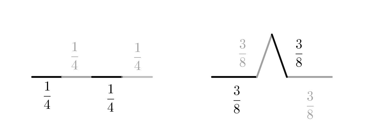
Let us fix $n=2$ and let $\delta\in(1,2)$. The von Koch curve construction can be modify so that the resulting curve has a Hausdorff dimension of $\delta$ and a positive $\delta$-dimension Hausdorff measure, see [22, Section 3]. This happens by dividing a line segment $K$ into four equally long segments, and replacing each subsegment with a segment of length $s|K|$, for a fixed $s\in(\frac{1}{4},\frac{1}{2})$, in such a way that the segments $K_{0}$ and $K_{3}$ are subsets of $K$ at opposite ends of $K$, and $K_{1}$ and $K_{2}$ are the sides of an isosceles triangle whose base is $K\setminus(K_{0}\bigcup K_{3})$. This gives a curve with the Hausdorff dimension $\frac{\log(4)}{\log(1/s)}$.

Refer to caption
Refer to caption
Figure 1. Pictures on the left-hand side and in the middle : An example of the construction of the modified von Koch’s curve, where $s=\frac{3}{8}$. The picture is a modification of [22, Figure 1]. The right-hand side domain: An open set $\Omega$ bounded by three modified von Koch’s curves.

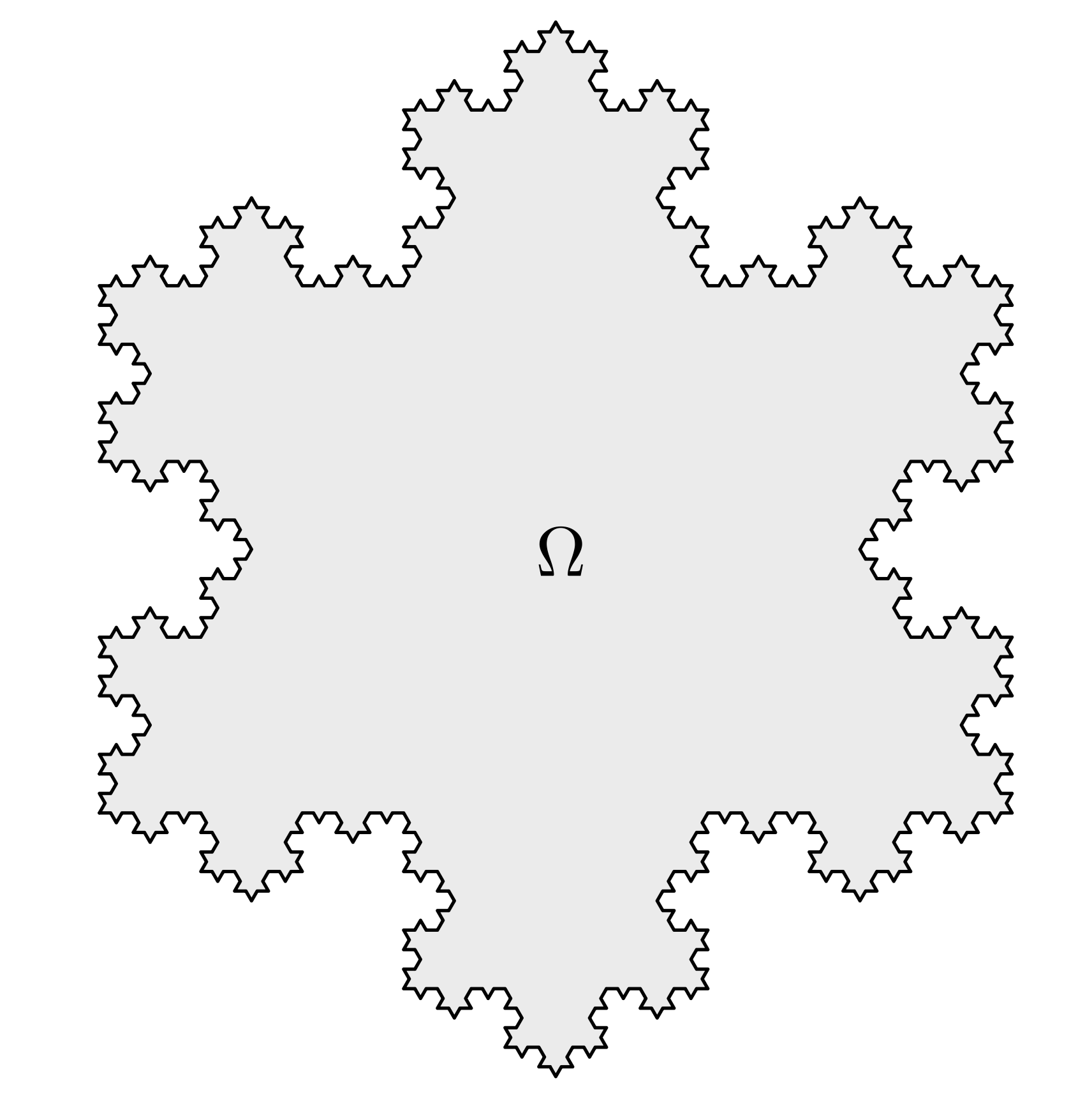
By joining three these curves together we obtain the von Koch snowflake $F$, which bounds an open set $\Omega$. This means that $F=\partial\Omega$. We show that for all points $x\in F$ we have

$$\chi_{\Omega}(x)\neq\limsup_{r\to 0^{+}}(\chi_{\Omega})_{B(x,r)}^{\delta}.$$

Clearly $\chi_{\Omega}(x)=0$ for all $x\in F$. By the construction of the von Koch curve there exists $c\in(0,1)$, depending on $\delta$, such that every $x\in F$ and every $0<r<\mathop{diam}\nolimits(\Omega)/2$ there exists $y\in\Omega$ such that $B(y,cr)\subset\Omega\cap B(x,r)$. Calculations as in Example 6.1 imply that

$$\chi_{\Omega}(x)=0<c_{1}c^{\delta}\leq\limsup_{r\to 0^{+}}(\chi_{\Omega})_{B(x,r)}^{\delta}$$

for all points $x\in F$, and $\tilde{\mathcal{H}}^{\delta}_{\infty}(F)>0$. Moreover, the characteristic function $\chi_{\Omega}$ is a Lebesgue measurable function which belongs to ${\textsc{n}L}^{1}({\varmathbb{R}^{n}},\tilde{\mathcal{H}}^{\delta}_{\infty})$. Thus (5.13) does not hold, and hence by Theorem 5.11 the function $\chi_{\Omega}\in{\textsc{n}L}^{1}(\varmathbb{R}^{2},\tilde{\mathcal{H}}^{\delta}_{\infty})$  is not an ${\textsc{n}L}^{1}$-limit of continuous functions.

6.3 Remark.

Let $0<\delta<n$ be fixed. Examples 6.1 and 6.2 show that in the function space ${\textsc{n}L}^{1}({\varmathbb{R}^{n}},\tilde{\mathcal{H}}^{\delta}_{\infty})$ there exist Lebesgue measurable functions which are not ${\textsc{n}L}^{1}$-limits of continuous functions. This implies two remarkable conclusions:

  1. (1)

    if $\delta<n$, then continuous functions are not dense in ${\textsc{n}L}^{1}({\varmathbb{R}^{n}},\tilde{\mathcal{H}}^{\delta}_{\infty})$;

  2. (2)

    the assumption $\delta=n$ in Theorem 5.9 (1) is necessary.

References

  • [1] Adams, D. R.: A note on Riesz potentials, Duke Math. J.  42 (1975), no. 4, 765–778.
  • [2] Adams, D. R.: A note on Choquet integrals with respect to Hausdorff capacity. In: Cwikel, M., Peetre, J., Sagher, Y., Wallin, H. (eds.) Function Spaces and Applications (Lund 1986), Lecture Notes in Mathematics vol. 1302, Springer, Berlin (1988) pp. 115–124.
  • [3] Adams, D. R.: Choquet Integrals in Potential Theory, Publ. Mat.  42 (1998), 3–66.
  • [4] Adams, D. R.: Morrey Spaces, Birkhäuser, Cham–Heidelberg–New York, 2015.
  • [5] Adams, D. R., Xiao, J.: Bochner–Riesz means of Morrey functions, J. Fourier Anal. Appl. 26 (2020), no. 1, Paper No. 7.
  • [6] Adams, R. A.: Sobolev Spaces, Academic Press, Inc., London, 1975.
  • [7] Basak, R., Chen, Y.-W. B., Roychowdhury, P. and Spector, D.: The capacitary John–Nirenberg inequality revisited, https://arxiv.org/abs/2501.11412
  • [8] Cerdá, J., Martín, J., Silvestre, P.: Capacitary function spaces. Collect. Math. 62 (2011), no. 1, 95–118.
  • [9] Chen, Y.-W., Ooi, K.H., Spector, D.: Capacitary maximal inequalities and applications. J. Funct. Anal.  286 (2024), issue 12, paper no. 110396.
  • [10] Chen, Y.-W., Spector, D.: On functions of bounded $\beta$-dimensional mean oscillation, Adv. Calc. Var. 17 (2024), no. 3, 273-296.
  • [11] Choquet, G.: Theory of capacities. Ann. Inst. Fourier (Grenoble) 5 (1953–1954), 13–295.
  • [12] Dafni, G., Xiao, J.: Some new tent spaces and duality theorems for fractional Carleson measures and $Q_{\alpha}({\varmathbb{R}^{n}})$, J. Funct. Anal. 208 (2004), 377–422.
  • [13] Denneberg, D.: Non-additive measure and integral, Theory and Decision Library Series B: Mathematical and Statistical Methods vol. 27, Kluwer Academic Publishers Group, Dordrecht, 1994.
  • [14] Garcia Cuerva, J. L., Rubio de Francia, J. L.: Weighted norm inequalities and related topics, Mathematics Studies 116, North Holland, Amsterdam, 1985.
  • [15] Folland, G.: Real Analysis: modern techniques and applications, $2^{nd}$edition, Pure and Applied Mathematics: A Wiley-Interscience Series of Text, Monographs, and Tracts, John Wiley& Sons, Inc., New York, 1999.
  • [16] Halmos, P. R.: Measure Theory, Graduate Texts in Mathematics, volume 18, Springer Science+Business Media, New York, 1950.
  • [17] Harjulehto, P., Hurri-Syrjänen, R.: On Choquet integrals and Poincaré-Sobolev type inequalities, J. Funct. Anal. 284 (2023), issue 9, paper no. 109862.
  • [18] Harjulehto, P., Hurri-Syrjänen, R.: Estimates for the variable order Riesz potential with application. In: Lenhart, S., Xiao, J. (eds.) Potentials and Partial Differential Equations: The Legacy of David R. Adams, Advances in Analysis and Geometry vol. 8, De Gruyter, Berlin (2023) pp. 127–155.
  • [19] Harjulehto, P., Hurri-Syrjänen, R.: On Choquet integrals and pointwise estimates, Proceedings of 2022 AWM Research Symposium, Association for Women in Mathematics Series, accepted.
  • [20] Harjulehto, P., Hurri-Syrjänen, R.: On Choquet integrals and Sobolev type inequalities, La Matematica 3 (2024), 1379-1399, doi:10.1007/s44007-024-00131-z.
  • [21] Harjulehto, P., Hurri-Syrjänen, R.: On Hausdorff content maximal operator and Riesz potential for non-measurable functions, submitted manuscript.
  • [22] Harjulehto, P., Hästö, P., Latvala, V.: Sobolev embeddings in metric measure spaces with variable dimension, Math. Z. 254 (2006), no. 3, 591–609.
  • [23] Hildebrandt, T. H.: On integrals related to and extensions of the Lebesgue integrals. Bull. Amer. Math. Soc. 24 (1917), no. 3, 113–144.
  • [24] Huang, L., Cao, Y., Yang, D., Zhuo, C.: Poincaré-Sobolev inequalities based on Choquet-Lorentz integrals with respect to Hausdorff contents on bounded John domains. arXiv:2311.15224.
  • [25] Jeffery, R. L.: Relative summability, Ann. of Math. (2) 33 (1932), no. 3, 443–459.
  • [26] Kawabe, J.: Convergence in Measure Theorems of the Choquet Integral Revisited. Modeling decisions for artificial intelligence, Lecture Notes in Comput. Sci. 11676 Lecture Notes in Artificial Intelligence, Springer Cham (2019) pp. 17–28.
  • [27] Kinnunen, J.: Real Analysis, lectures notes,
    https://sites.google.com/view/jkkinnun/
  • [28] Martínez, Á. D., Spector, D.: An improvement to the John-Nirenberg inequality for functions in critical Sobolev spaces. Adv. Nonlinear Anal. 10 (2021), 877–894.
  • [29] Ooi, K. H., Phuc, N. C.: The Hardy-Littlewood maximal function, Choquet integrals, and embeddings of Sobolev type, Math. Ann. 382 (2022), 1865–1879.
  • [30] Orobitg, J., Verdera, J.: Choquet integrals, Hausdorff content and the Hardy-Littlewood maximal operator. Bull. London Math. Soc. 30 (1998), 145–150.
  • [31] Ponce, A. C.: Elliptic PDEs, Measures and Capacities, Tracts in Mathematics 23, European Mathematical Society, Bad Lagensalza, Germany, 2016.
  • [32] Ponce, A., Spector, D.: A boxing inequality for the fractional perimeter. Ann. Sc. Norm. Super. Pisa Cl. Sci.(5) 20 (2020), 107–141.
  • [33] Ponce, A., Spector, D.: Some remarks on Capacitary Integrals and Measure Theory. In: Lenhart, S., Xiao, J. (eds.) Potentials and Partial Differential Equations: The Legacy of David R. Adams, Advances in Analysis and Geometry vol. 8, De Gruyter, Berlin (2023) pp. 127–155.
  • [34] Saito, H.: Boundedness of the strong maximal operator with the Hausdorff content, Bull. Korean Math. Soc. 56 (2019), no. 2, 399–406.
  • [35] Saito, H., Tanaka, H.: Dual of the Choquet spaces with general Hausdorff content. Studia Math. 266 (2022), no. 3, 323–335.
  • [36] Saito, H., Tanaka, H., Watanabe, T.: Abstract dyadic cubes, maximal operators and Hausdorff content. Bull. Sci. Math. 140 (2016), no. 6, 757–773.
  • [37] Saito, H., Tanaka, H., Watanabe, T.: Fractional maximal operators with weighted Hausdorff content. Positivity 23 (2019), no. 1, 125–138.
  • [38] Song, L., Xiao, J., Yan, X.: Preduals of quadratic Campanato spaces associated to operators with heat kernel bounds, Potential. Anal. 41 (2014), no 3, 849–867.
  • [39] Tang, L.: Choquet integrals, weighted Hausdorff content and maximal operators, Georgian Math. J. 18 (2011), 587–596.
  • [40] Vitali, G.: Sul Problema della misura dei grupp di punti di una retta, Bologna, Tip. Gamberini e Parmeggiani, (1905).
  • [41] Watanabe, H.: Estimates of maximal functions by Hausdorff content in a metric space, Advanced Studies in Pure Mathematics 44, 2006, Potential Theory in Matsue, 377-389.
  • [42] Yang D., Yuan, W.: A note on dyadic Hausdorff capacities, Bull. Sci. Math. 132 (2008), 500–509.
  • [43] Zakon, E.: Integration of non-measurable functions, Canad. Math. Bull. 9 (1966), 307–330.
  • [44] Ziemer, W. P.: Weakly Differentiable Functions, Graduate Texts in Mathematics, 120, Springer-Verlag, New York, 1989.