\ul
General Time-series Model for Universal Knowledge Representation of Multivariate Time-Series data
Abstract
Universal knowledge representation is a central problem for multivariate time series(MTS) foundation models and yet remains open. This paper investigates this problem from the first principle and it makes four folds of contributions. First, a new empirical finding is revealed: time series with different time granularities (or corresponding frequency resolutions) exhibit distinct joint distributions in the frequency domain. This implies a crucial aspect of learning universal knowledge, one that has been overlooked by previous studies. Second, a novel Fourier knowledge attention mechanism is proposed to enable learning time granularity-aware representations from both the temporal and frequency domains. Third, an autoregressive blank infilling pre-training framework is incorporated to time series analysis for the first time, leading to a generative tasks agnostic pre-training strategy. To this end, we develop the General Time-series Model (GTM), a unified MTS foundation model that addresses the limitation of contemporary time series models, which often require token, pre-training, or model-level customizations for downstream tasks adaption. Fourth, extensive experiments show that GTM outperforms state-of-the-art (SOTA) methods across all generative tasks, including long-term forecasting, anomaly detection, and imputation.
Keywords Machine Learning Multivariate Time Series Foundation Model Multi-tasks adaption
1 Introduction
Recently, there is a surge of interests in time series foundation models that can accommodate diverse data domains and support a wide range of downstream tasks [1, 2]. There are two typical categories of MTS downstream tasks: (1) generative tasks including forecasting, imputation and anomaly detection; (2) predictive tasks including classification [2].
One central question in building MTS foundation model is universal knowledge representation, and yet it still remains open [2]. Formal definition of universal knowledge of MTS is still missing. The dominant paradigm is to encode MTS knowledge within a black-box model, with downstream task performance serving as the golden metric[3, 4, 5, 6, 2]. The development of methodologies is driven by understanding the multifaceted nature of MTS, where the time domain captures temporal variation, and the frequency domain depicts amplitude and phase variation.
In the task-specific knowledge representation setting, both the time domain and frequency domain are extensively studied [7, 8, 9, 10]. Deep learning models, especially Transformer-based models, have demonstrated strong representational capabilities, as evidenced by their effectiveness in capturing long-range dependencies[7, 8]. Recent studies have highlighted the advantages of combining both temporal and frequency domain information for enhanced performance [9, 10]. However, this kind of knowledge is far from universal, as these models often struggle with adaptability across diverse domains and are typically tailored to specific tasks.
A number of MTS foundation models made notable progress in mitigating the aforementioned adaptivity limitation through exploiting the temporal domain. One typical line of works freeze LLM encoder backbones while simultaneously fine-tuning/adapting the input and distribution heads for downstream tasks. Its effectiveness is currently under debating in the sense that positive progress was reported such as Time-LLM[11], LLM4TS[12], GPT4TS[3], UniTime[13] and Tempo[14], while latest ablation studies showed the counterpart [15]. Another line of works train MTS foundation models from scratch [2, 16]. For the forecasting task, a number time-series foundation model were shown to have nice adaptivity to diverse data domains [4, 5, 6]. Furthermore, several recent time-series foundation models have shown the ability to adapt to a wide range of generative tasks, including forecasting, imputation, and anomaly detection, simultaneously[16, 17]. Others are even capable of extending across both generative tasks (e.g., forecasting) and classification tasks[18, 19]. However, the adaptability of contemporary multi-task foundation models faces a ’last-mile’ bottleneck, as they often require token-level, pre-training strategy-level, or model-level customizations for downstream tasks. For instance, Timer[16] offers three pre-training strategies to accommodate down stream tasks, while UP2ME[17] introduces specialized TC layers for task-specific fine-tuning to achieve improved performance
This paper investigates universal knowledge representation in MTS data from the first principle. Specifically, we begin by examining what additional aspects or features contribute to a more complete universal representation—a question often overlooked by contemporary MTS foundation models. While both temporal and frequency domain information have been shown to contribute to task-specific ones, we question their sufficiency in achieving a more comprehensive results. Our findings reveal new dimensions of universal knowledge representation, which inspire the design of the GTM model, enhancing its capabilities for both knowledge representation and adaptivity. Our contributions are:
(1) New findings in the knowledge of MTS data. We show that besides conventional temporal domain and frequency domain information, time granularity is a crucial factor for universal knowledge representation.
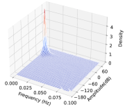
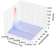
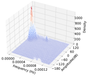
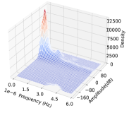
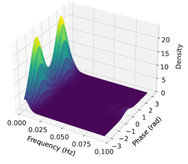
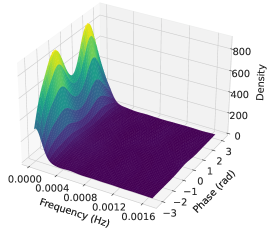
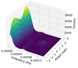
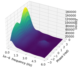
We use FFT and statistical techniques to analyzed large-scale time series datasets like UTSD-12G [16] (details of the analysis is presented in Section A.4.1). Figure 1 shows the joint distribution of frequency and amplitude extracted from time series with varying time granularities. It is evident that time series with different time granularities exhibit distinct joint density distributions over the amplitude-frequency pair, as well as phase-frequency pair. This finding highlights the importance of time granularities as intrinsic elements of time series knowledge, which, however, are overlooked by all contemporary time series foundation models.
(2) Frequency and time granularity aware backbone design. Inspired by the aforementioned findings, we propose an -stack Decoder-Only Backbone with low-rank modules to implement a frequency domain knowledge attention mechanism, enhancing universal knowledge representation of MTS data with varying time granularities. To the best of our knowledge, this is the first MTS foundation model to integrate Fourier Knowledge Attention modules, enabling the learning of time granularity-aware, universal representations from both the temporal and frequency domains.
(3) Unified pre-training strategy. We introduce an autoregressive blank infilling pre-training framework from the LLM field, adapted for MTS analysis, with a unified linear projection header to generate output data autoregressively. This strategy solves the ’one task, one model’ challenge, overcoming the limitations of MTS foundation models, which often require customizations at the token, model, or pre-training level for downstream tasks.
(4) Extensive evaluation. We conducted extensive experiments comparing GTM with state-of-the-art (SOTA) models across typical generative downstream tasks, like forecasting, anomaly detection, and imputation. The results show that GTM outperforms baseline methods in nearly all aspects, further validating our findings and design principles.
2 Related works
Due to page limit, we focus primarily on MTS foundation models trained from scratch, additional literature review and comparison can be found in Section A.1.
| Time Series Features | Downstream Tasks | Adaptivity | |||||||||
|---|---|---|---|---|---|---|---|---|---|---|---|
| Temporal Domain | Freq. Domain | Time Gran. | Forecasting | Anomaly Detection | Imputation | CLF. | W/o inference adaption | ||||
|
|||||||||||
| TimeSiam, LPTM | |||||||||||
| TIMER, UP2ME | |||||||||||
| UniTS | |||||||||||
| GTM(ours) | |||||||||||
Early attempts. TimesNet[1] achieves good performance across various generative downstream tasks. The idea of adding a new dimension of multi-periodicity to temporal modeling is a novel approach, proving effective for enabling multi-task adaption. PatchTST[20] unlocks the potential of Transformer for MTS forecasting. Two pioneering components, i.e., Channel Independence and Patching, were introduced to Transformer, opening new possibilities for time series foundation models.
MTS foundation model for forecasting. This line of works focus only on the forecasting task, aiming to enable adaptivity to diverse data domains. Lag-Llama[4] is one effort in this research line. Built on decoder-only architecture that incorporates lags as covariates and constructs features from timestamps, Lag-Llama has been shown to outperform previous deep learning approaches through fine-tuning on relatively small subsets of unseen datasets. GPHT[21] extends PatchTST by incorporating a hierarchical decoder-only backbone and employs an auto-regressive forecasting approach. One key advantage of GPHT is its ability to forecast across arbitrary horizon settings with a single model. TimesFM [22] is based on stacked decoder-only transformer backbone with patching. With 200M parameters and pretraining on data points, it yields accurate zero-shot forecasts across different domains, forecasting horizons and temporal granularities. GPD[23] and UTSD [24] aim to address the across-domain issue of MTS forecasting. They utilize diffusion models to model the mixture distribution of the cross-domain data. MOIRAI [25] is built on a masked encoder-only Transformer backbone, but specially focus on tackling the cross-frequency learning challenge and accommodating an arbitrary number of variates for MTS. The idea of flattening the MTS into a single sequence is novel, which enables it to learn multivariate interactions while considering exogenous covariates. TTMs [5] reduces the computational cost of existing models while capturing cross-channel and exogenous correlations that are often missed by traditional approaches. TIME-MOE[6] also reduces the computational cost by using a decoder-only forecasting model with a sparse mixture-of-experts (MOE) design. During training, it optimizes forecasting heads at multiple resolutions with varying prediction lengths, and dynamically schedules these heads for flexible forecasting during inference.
Multi-task MTS foundation model. This line of works aim to enable adaptivity to a wide range of down stream tasks. UP2ME[17] is built on a Transformer backbone and uses Masked AutoEncoder for pre-training. It introduces two instance generation techniques: variable window lengths and channel decoupling to remove cross-channel dependencies. During fine-tuning, it employs a Graph Transformer, freezing the backbone parameters while adding learnable Temporal-Channel (TC) layers. Timer[16] is built on a decode-only backbone and uses autoregressive approach with causal attention for generative pre-training. It defines a unified single-series sequence(S3) data format to curate 1 billion time points datasets for pre-training. Its pre-training approach fits well with forecasting and prediction-based anomaly detection tasks, but can’t provide sufficient context information in imputation task. TimeSiam [18] and LPTM[19] are tailored to time series forecasting and classification tasks. TimeSiam uses the Siamese networks (Bromley et al., 1993) as its backbone and employs contrastive learning for pretraining. It aims to address the challenge that randomly masking time series or calculating series-wise similarity can distort or neglect the inherent temporal correlations that are critical in time series data. While contrastive learning enhances its performance in certain tasks, it results in limited adaptability for generative tasks. LPTM[19] aims to address the cross-domain challenge of extracting semantically meaningful tokenized inputs from heterogeneous time series across different domains. It combines a Transformer and GRU as its backbone and employs an adaptive segmentation method that automatically identifies the optimal segmentation strategy during pretraining. However, like TimeSiam, it has limited adaptability for generative tasks. UniTS [2] is designed to handle both generative and classification tasks simultaneously. It uses task tokenization to integrate these tasks into a unified framework. The model employs a modified transformer block with two separate towers: one tailored for classification tasks and the other for generative tasks. This design enables effective transfer from a heterogeneous, multi-domain pretraining dataset to a variety of downstream datasets with varied task specifications and data domains.
Summary of difference. Table1 summarizes the key differences between our work and the above models. First, previous foundation models rely only on temporal information from discrete scalar values, while ours utilize both temporal and frequency domain information. Second, previous models require token, pre-training strategy or model level customization for down stream tasks, while ours does not due to new pre-training strategy design. Finally, our work introduces two architectural innovations: the Fourier Knowledge Attention mechanism, which learns time granularity-aware representations from both domains, and an autoregressive blank infilling pre-training framework, enabling a generative task-agnostic pre-training strategy.
3 Method
3.1 Design Overview
We denote An MTS by where and denote the number of timestamps and variates respectively. We consider an MTS dataset, UTSD-12G, which comprises of a large number of MTS from diverse application domains.
GTM is pre-trained on this dataset from scratch, aiming to support generative tasks, such as forecasting, imputation and anomaly detection, simultaneously. Fig.2 illustrates the architecture of GTM.
Input data embedding. Reversible Instance Normalization[26], Channel Independence (CI), Patching[20] and Masking[27] techniques are applied to transform raw MTS data into univariate masked token sequences. We also incorporate linear embedding and positional embedding before feeding these tokens into the model backbone.
N-stack Decoder-only backbone.
We adopt a decoder-only framework as the backbone architecture for generating output autoregressively. To enhance the representation and knowledge learning of MTS data in both the temporal and frequency domains, we preserve the temporal self-attention module while re-design the Fourier attention module, which will be elaborated in the subsection 3.2.
Output projection. Mainstream models typically use a flatten layer with a linear head for one-step generation. This design requires modifying the output layer for different downstream tasks, hindering the reuse of pre-trained parameters and knowledge. To overcome this limitation, we unify the output layer for both pretraining and downstream tasks by using a direct linear projection and instance denormalization to generate output autoregressively.
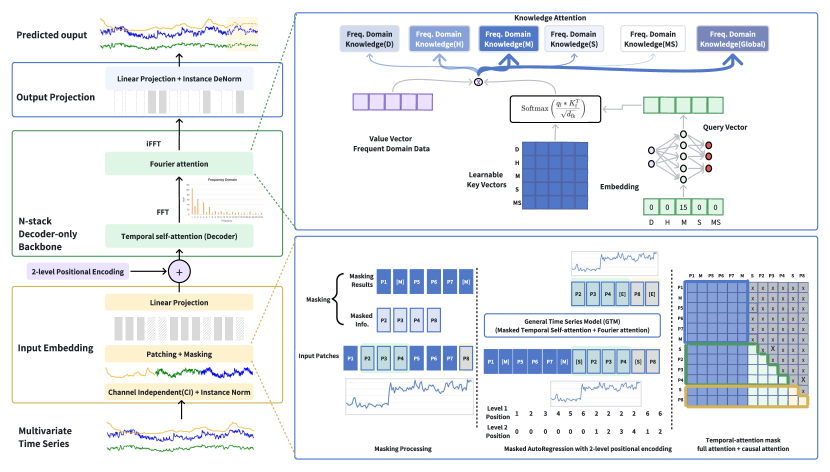
3.2 The -stack Decoder-only Backbone
We propose an -stack decoder-only backbone that enhances the representation of MTS data by integrating temporal and frequency attention. GTM combines a standard temporal self-attention layer with a modified Fourier attention block to capture frequency domain knowledge using data processed via Fast Fourier Transform (FFT). Unlike the MoE[28] architecture, our design is closer to a knowledge attention mechanism, incorporating various frequency domain knowledge modules to learn distinct joint distributions of MTS with vary time granularities. We propose a time-granularity aware representation that captures all temporal granularity information in a quintuple format, where each element represents day, hour, minute, second, and millisecond. For instance, the time granularity of the ETTm dataset[29] is represented as [0, 0, 15, 0, 0], which is then transformed into a query vector through linear embedding. We also initiate five learnable vectors as key vectors for each granularity, and compute attention scores with the softmax function to weigh the importance of the corresponding knowledge matrices. Additionally, a global frequency knowledge module runs in parallel, representing overall frequency domain knowledge without frequency resolution and is always activated with a probability of 1.
Temporal & Fourier Attention.
The temporal self-attention module takes as input, which is obtained by performing the input embedding on . The output is:
| (1) |
where and denote weight matrices. Each column of is a temporal patch, and FFT is applied to transform each path into frequency domain signals:
| (2) |
Six frequency domain knowledge modules are designed afterwards, including five modules with low ranking parameters, denoted as , and one full connection layer with weight matrix . We define key matrix with five learnable vectors represents five different time granularity as . Query vector represents specific time granularity, yielding where denotes the weight matrix for query vector. We can then obtain the Fourier attention results using Eq. 3, along with the representation of one layer after the iFFT transformation, :
| (3) | |||
| (4) |
The stack decoder-only backbone yields:
| (5) |
where denote the index of layer and the the first layer takes as input, i.e., .
Output Projection. We use unified linear projection to generate output patches autoregressively where denotes linear projection weight. In this manner, except for special cases, the GTM model can adapt to various downstream tasks without requiring any modifications to the network architecture.
3.3 Pre-training Framework
The MTS is devided into patches following the ideas of CI and Patching[20]. Each row of is processed independently. The -th row of is divided into overlapping windows of data points with a stride and length . Formally, the -th windows of data points denoted by can be expressed as The is divided into patches forming a patch matrix :
GLM [27] proposes an autoregressive blank infilling pre-training framework for various NLP tasks. Inspired by this, we adapt and develop a general masking process for generative task-agnostic MTS analysis, as shown in Fig.2. Each patch span consists of one or more consecutive patches, and patch spans are randomly sampled from denoted by:
Fig.2 illustrates an example, where , and . Each sampled patch span is replaced by a single [MASK] token to form a corrupted patch denoted by , formally
In this example, .
| Models | GTM | GPT4TS | UniTS-PMT | PatchTST | TimesNet | DLinear | FEDformer | Autoformer | Informer | ||||||||||||
|---|---|---|---|---|---|---|---|---|---|---|---|---|---|---|---|---|---|---|---|---|---|
| dataset | pred_len | MSE | MAE | MSE | MAE | MSE | MAE | MSE | MAE | MSE | MAE | MSE | MAE | MSE | MAE | MSE | MAE | MSE | MAE | MSE | MAE |
| 96 | 0.360 | \ul0.398 | 0.376 | 0.397 | 0.390 | 0.411 | \ul0.363 | - | 0.370 | 0.400 | 0.384 | 0.402 | 0.375 | 0.399 | 0.376 | 0.415 | 0.435 | 0.446 | 0.865 | 0.713 | |
| 192 | \ul0.397 | 0.422 | 0.416 | \ul0.418 | 0.432 | 0.438 | 0.394 | - | 0.413 | 0.429 | 0.436 | 0.429 | 0.405 | 0.416 | 0.423 | 0.446 | 0.456 | 0.457 | 1.008 | 0.792 | |
| ETTh1 | 336 | \ul0.420 | \ul0.437 | 0.442 | 0.433 | 0.480 | 0.460 | 0.403 | - | 0.422 | 0.440 | 0.491 | 0.469 | 0.439 | 0.443 | 0.444 | 0.462 | 0.486 | 0.487 | 1.107 | 0.809 |
| 720 | 0.438 | \ul0.457 | 0.477 | 0.456 | 0.542 | 0.508 | 0.449 | - | \ul0.447 | 0.468 | 0.521 | 0.500 | 0.472 | 0.490 | 0.469 | 0.492 | 0.515 | 0.517 | 1.181 | 0.865 | |
| Avg | \ul0.404 | \ul0.429 | 0.427 | 0.426 | 0.461 | 0.454 | 0.402 | - | 0.413 | 0.434 | 0.458 | 0.450 | 0.422 | 0.437 | 0.428 | 0.453 | 0.473 | 0.476 | 1.040 | 0.795 | |
| 96 | 0.282 | 0.341 | \ul0.292 | 0.346 | - | - | 0.293 | - | 0.293 | 0.346 | 0.338 | 0.375 | 0.299 | \ul0.343 | 0.326 | 0.390 | 0.510 | 0.492 | 0.672 | 0.571 | |
| 192 | 0.325 | \ul0.366 | \ul0.332 | 0.372 | - | - | 0.335 | - | 0.333 | 0.370 | 0.374 | 0.387 | 0.335 | 0.365 | 0.365 | 0.415 | 0.514 | 0.495 | 0.795 | 0.669 | |
| ETTm1 | 336 | 0.353 | 0.385 | 0.366 | 0.394 | - | - | \ul0.364 | - | 0.369 | 0.392 | 0.410 | 0.411 | 0.369 | \ul0.386 | 0.392 | 0.425 | 0.510 | 0.492 | 1.212 | 0.871 |
| 720 | 0.396 | 0.410 | 0.417 | 0.421 | - | - | 0.408 | - | \ul0.416 | \ul0.420 | 0.478 | 0.450 | 0.425 | 0.421 | 0.446 | 0.458 | 0.527 | 0.493 | 1.166 | 0.823 | |
| Avg | 0.339 | 0.376 | 0.352 | 0.383 | - | - | \ul0.350 | - | 0.352 | 0.382 | 0.400 | 0.406 | 0.357 | \ul0.378 | 0.382 | 0.422 | 0.515 | 0.493 | 0.961 | 0.734 | |
| 96 | 0.147 | 0.197 | 0.162 | 0.212 | 0.157 | 0.206 | 0.154 | - | \ul0.149 | \ul0.198 | 0.172 | 0.220 | 0.176 | 0.237 | 0.238 | 0.314 | 0.249 | 0.329 | 0.300 | 0.384 | |
| 192 | 0.192 | 0.241 | 0.204 | 0.248 | 0.208 | 0.251 | 0.207 | - | \ul0.194 | \ul0.241 | 0.219 | 0.261 | 0.220 | 0.282 | 0.325 | 0.370 | 0.325 | 0.370 | 0.598 | 0.544 | |
| weather | 336 | \ul0.250 | 0.291 | 0.254 | \ul0.286 | 0.264 | 0.291 | 0.250 | - | 0.245 | 0.282 | 0.280 | 0.306 | 0.265 | 0.319 | 0.351 | 0.391 | 0.351 | 0.391 | 0.578 | 0.523 |
| 720 | 0.310 | 0.334 | 0.326 | 0.337 | 0.344 | 0.344 | 0.324 | - | \ul0.314 | \ul0.334 | 0.365 | 0.359 | 0.323 | 0.362 | 0.415 | 0.426 | 0.415 | 0.426 | 1.059 | 0.741 | |
| Avg | 0.225 | \ul0.266 | 0.237 | 0.270 | 0.243 | 0.273 | 0.234 | - | \ul0.225 | 0.263 | 0.259 | 0.287 | 0.246 | 0.300 | 0.332 | 0.375 | 0.335 | 0.379 | 0.634 | 0.548 | |
| 96 | 0.351 | \ul0.250 | 0.388 | 0.282 | 0.465 | 0.298 | 0.372 | - | \ul0.360 | 0.249 | 0.593 | 0.321 | 0.410 | 0.282 | 0.576 | 0.359 | 0.597 | 0.371 | 0.719 | 0.391 | |
| 192 | \ul0.373 | \ul0.260 | 0.407 | 0.290 | 0.484 | 0.306 | 0.365 | - | 0.379 | 0.256 | 0.617 | 0.336 | 0.423 | 0.287 | 0.610 | 0.380 | 0.607 | 0.382 | 0.696 | 0.379 | |
| traffic | 336 | \ul0.388 | \ul0.267 | 0.412 | 0.294 | 0.494 | 0.312 | 0.379 | - | 0.392 | 0.264 | 0.629 | 0.336 | 0.436 | 0.296 | 0.608 | 0.375 | 0.623 | 0.387 | 0.777 | 0.420 |
| 720 | \ul0.428 | \ul0.288 | 0.450 | 0.312 | 0.534 | 0.335 | 0.425 | - | 0.432 | 0.286 | 0.640 | 0.350 | 0.466 | 0.315 | 0.621 | 0.375 | 0.639 | 0.395 | 0.864 | 0.472 | |
| Avg | 0.385 | \ul0.266 | 0.414 | 0.294 | 0.494 | 0.313 | \ul0.385 | - | 0.390 | 0.263 | 0.620 | 0.336 | 0.433 | 0.295 | 0.603 | 0.372 | 0.616 | 0.383 | 0.764 | 0.416 | |
| 96 | 0.131 | \ul0.225 | 0.139 | 0.238 | 0.157 | 0.258 | 0.129 | - | \ul0.129 | 0.222 | 0.168 | 0.272 | 0.140 | 0.237 | 0.186 | 0.302 | 0.196 | 0.313 | 0.274 | 0.368 | |
| 192 | 0.149 | \ul0.243 | 0.153 | 0.251 | 0.173 | 0.272 | \ul0.148 | - | 0.147 | 0.240 | 0.184 | 0.289 | 0.153 | 0.249 | 0.197 | 0.311 | 0.211 | 0.324 | 0.296 | 0.386 | |
| Electricity | 336 | 0.166 | 0.259 | 0.169 | 0.266 | 0.185 | 0.284 | \ul0.161 | - | 0.163 | \ul0.259 | 0.198 | 0.300 | 0.169 | 0.267 | 0.213 | 0.328 | 0.214 | 0.327 | 0.300 | 0.394 |
| 720 | 0.201 | \ul0.292 | 0.206 | 0.297 | 0.219 | 0.314 | 0.193 | - | \ul0.197 | 0.290 | 0.220 | 0.320 | 0.203 | 0.301 | 0.233 | 0.344 | 0.236 | 0.342 | 0.373 | 0.439 | |
| Avg | 0.161 | \ul0.254 | 0.167 | 0.263 | 0.184 | 0.282 | 0.158 | - | \ul0.159 | 0.252 | 0.192 | 0.295 | 0.166 | 0.263 | 0.207 | 0.321 | 0.214 | 0.326 | 0.311 | 0.397 | |
The sampled patch spans are randomly permuted. Special tokens [START] and [END] are padded to each of sampled span forming input and label data:
| (6) | |||
| (7) |
where denotes a random permutation over . The goal of the pre-training is to autoregressively reconstruct all masked patches (Eq.8), minimizing the discrepancy(MSE) compared with ground-truth Eq.(9).
| (8) | |||
| (9) |
where and denote the -th row of and .
Since [START] and [END] do not exist in the time-series analysis domain, we employ learnable vectors to represent them. To better adapt to various generative tasks, we set the proportion to apply all the [MASK] tokens to the consecutive patches at the tail of the input data. This strategy makes the generation of the masked patches more akin to a forecasting task. By combining these techniques, we overcome the limitations of SOTA models that rely on either mask reconstruction or the autoregressive method for pre-training. After trainable linear embedding , We also leverage the 2D learnable positional encoding method [27] to ensure that the backbone model is aware of the length of the masked span when generating output patches. Based on masking process, the input data is and it is fed into the backbone network for attention-based processing:
| (10) |
where and denotes 1D and 2D position coding matrix. In this manner, the GTM_Decoder backbone module can apply full-attention mask for , while causal attention mask for .
3.4 Fine-tuning for Downstream Tasks
Benefit from the model design and pre-training strategy, GTM can adapt to various generative downstream tasks without changes to the network architecture, apart from minor pre-processing adjustments, such as removing the masking process and 2D positional encoding. This makes GTM a versatile, pre-trained time series model capable of delivering high-precision results, as demonstrated in Sec. 4.
4 Experiments
We present extensive experiments evaluating our proposed GTM model, comparing it with different kinds of SOTA models (details are listed in Appendix A.2.2) to highlight the performance improvements achieved by our design. We also provide results from directly training the model for downstream tasks, demonstrating that pre-training on large-scale datasets yields additional performance gains. Finally, we conduct ablation studies to show the effectiveness of the key network modules.
| Models | GTM | GPT4TS | TimesNet | PatchTST | DLinear | Fedformer | Informer | |||||||
|---|---|---|---|---|---|---|---|---|---|---|---|---|---|---|
| dataset | MSE | MAE | MSE | MAE | MSE | MAE | MSE | MAE | MSE | MAE | MSE | MAE | MSE | MAE |
| ETTh1 | 0.053 | 0.152 | \ul0.069 | \ul0.173 | 0.078 | 0.187 | 0.115 | 0.224 | 0.201 | 0.306 | 0.117 | 0.246 | 0.161 | 0.279 |
| ETTm1 | 0.021 | 0.096 | 0.028 | \ul0.105 | \ul0.027 | 0.107 | 0.047 | 0.140 | 0.093 | 0.206 | 0.062 | 0.177 | 0.071 | 0.188 |
| weather | 0.030 | 0.054 | 0.031 | 0.056 | \ul0.030 | \ul0.054 | 0.060 | 0.144 | 0.052 | 0.110 | 0.099 | 0.203 | 0.045 | 0.104 |
| Electricity | \ul0.086 | \ul0.202 | 0.090 | 0.207 | 0.092 | 0.210 | 0.072 | 0.183 | 0.132 | 0.260 | 0.130 | 0.259 | 0.222 | 0.328 |
| Models | GTM | UP2ME | GPT4TS | TimesNet | PatchTST | FEDformer | DLinear | Autoformer | Informer |
| Dataset | F1(%) | F1(%) | F1(%) | F1(%) | F1(%) | F1(%) | F1(%) | F1(%) | F1(%) |
| MSL | 82.53 | - | 82.45 | 81.84 | 78.70 | 78.57 | 84.88 | 79.05 | \ul84.06 |
| SMAP | 77.57 | - | \ul72.88 | 69.39 | 68.82 | 70.76 | 69.26 | 71.12 | 69.92 |
| SWaT | 94.78 | 93.85 | \ul94.23 | 93.02 | 85.72 | 93.19 | 87.52 | 92.74 | 81.43 |
| SMD | \ul85.47 | 83.31 | 86.89 | 84.61 | 84.62 | 85.08 | 77.10 | 85.11 | 81.65 |
| PSM | 95.43 | 97.16 | 97.13 | 97.34 | 96.08 | \ul97.23 | 93.55 | 93.29 | 77.10 |
| Average | 87.01 | - | \ul86.72 | 85.24 | 82.79 | 84.97 | 82.46 | 84.26 | 78.83 |
4.1 Datasets description
We use the large-scale public time series dataset UTSD-12G for pre-training, ensuring no downstream task-related data is included to prevent leakage. For forecasting and imputation tasks, we use five widely used public datasets from [29], and for anomaly detection tasks, we utilize five popular labeled datasets from [30, 31, 32, 33]. The detailed statistics of all these public datasets are provided in Appendix A.2.1
4.2 Long-term Forecasting
For long-term forecasting, we select representative baselines and cite their results respectively. These SOTA models include the LLM-enhanced model GPT4TS[3], the multi-task time series foundation model UniTS-PMT[2], the task-specific time series foundation model , TimesNet[5, 1], the Transformer-based models PatchTST, FEDformer, Autoformer, Informer[20, 9, 29, 34], and the MLP-based model Dlinear[35]. Note that we choose baselines that match our experimental settings the most and exclude models that involve pre-training and fine-tuning on the same datasets for downstream tasks. The long-term forecasting lengths includes time points. We utilize MSE and MAE as evaluating metrics for long-term forecasting. Notable, GTM directly utilizes pre-trained model without any modifications. As shown in Table 2, GTM outperforms all the SOTA models, achieving the best result in 21 and second best in 22 out of total 50 tests. The second best model , achieves the best in 14 and second best in 15.
| Models | GTM | GTM no pretrain | ||
|---|---|---|---|---|
| dataset | MSE | MAE | MSE | MAE |
| ETTh1 | 0.404(+7.1%) | 0.429(+4.0%) | 0.435 | 0.447 |
| ETTm1 | 0.339(+3.4%) | 0.376(3.3%) | 0.351 | 0.389 |
| weather | 0.225(+7.8%) | 0.266(+8.0%) | 0.244 | 0.289 |
| traffic | 0.385(+0.5%) | 0.266(+0.8%) | 0.387 | 0.268 |
| electricity | 0.161(+1.2%) | 0.254(+0.8%) | 0.163 | 0.256 |
4.3 Imputation
We use the same publicly available datasets in forecasting tasks and follow the protocol proposed by [3] for imputation tasks. To align with benchmark settings, we apply point-wise missing ratios for interpolation, and directly use pre-trained model for fine-tuning, only omitting the patching process. The point-wise imputation baselines include GPT4TS, TimesNet, PatchTST, FEDformer, Informer and Dlinear. We conduct the task with varying missing data ratios of at the time-point level. Table 3 demonstrates that, even without patch preprocessing, GTM achieves significant performance improvements. Compared to the second best model, GTM gets a 23.1% reduction in MSE, 12.1% in MAE for ETTh1 data, and 25.0% reduction in MSE, 8.6% in MAE for ETTm1 data. More details are in Appendix A.3.1
| Models | GTM | GTM no pretrain | ||
|---|---|---|---|---|
| dataset | MSE | MAE | MSE | MAE |
| ETTh1 | 0.053(+3.6%) | 0.152(+2.5%) | 0.055 | 0.156 |
| ETTm1 | 0.021(+8.6%) | 0.096(+4.0%) | 0.023 | 0.100 |
| weather | 0.030(+11.7%) | 0.054(+14.2%) | 0.034 | 0.063 |
| Electricity | 0.086(+1.2%) | 0.202(+0.5%) | 0.087 | 0.203 |
| electricity | 0.161(1.2%) | 0.254(0.8%) | 0.163 | 0.256 |
| Models | GTM | GTM(w/o time _gra) | GTM(w/o fft) | ||||
|---|---|---|---|---|---|---|---|
| dataset | MSE | MAE | MSE | MAE | MSE | MAE | |
| ETTh1 | Avg. | 0.404(3.57%, 2.42%) | 0.429(2.28%,0.92%) | \ul0.414(1.19%) | \ul0.433(1.37%) | 0.419 | 0.439 |
| ETTm1 | Avg. | 0.339(2.87%,2.59%) | 0.376(2.08%,1.57%) | \ul0.348(0.29%) | \ul0.382(0.52%) | 0.349 | 0.384 |
| Weather | Avg. | 0.225(3.43%,2.60%) | 0.266(3.62%,3.27%) | \ul0.231(0.86%) | \ul0.275(0.36%) | 0.233 | 0.276 |
| Traffic | Avg. | 0.385(1.79%,0.52%) | 0.266(1.85%,1.12%) | \ul0.387(1.28%) | \ul0.269(0.74%) | 0.392 | 0.271 |
| Electricity | Avg. | 0.161(2.42%,1.23%) | 0.254(1.93%,1.17%) | \ul0.163(1.21%) | \ul0.257(0.77%) | 0.165 | 0.259 |
4.4 Anomaly Detection
In the anomaly detection tasks, we fine-tune the pre-trained GTM model in a self-supervised manner through data reconstruction without any additional adaptions. We use a common adjustment strategy[36] where data points with reconstruction errors exceeding a threshold are considered anomalies. The baselines include the multi-task foundation model UP2ME, TimesNet, the LLM-enhanced model GPT4TS, the transformer-based models PatchTST, FEDformer, Autoformer, Informer, and the MLP-based model Dlinear. As shown in Table 4, GTM achieves the highest F1 score improvement compared to all baselines, with gains ranging from 0.33% (GPT4TS) to 10.38% (Informer).
4.5 Effectiveness of Pre-training
By pre-training on large-scale, multi-scenario, and multi-time granular MTS data, GTM learns richer and more universal representations. We compare the performance of two models: the baseline GTM, trained directly on task-specific datasets with random initialization, and the fine-tuned GTM, which benefits from pre-training. This comparison highlights the effectiveness of the pre-training approach.
Tables 5 and 6 summarize the average experimental results of both models across all datasets used for long-term forecasting of varying lengths and for imputation with different data missing ratios. The results indicate that, for long-term forecasting tasks, fine-tuned GTM consistently outperforms the baseline GTM in every comparison. It achieves a reduction in MSE ranging from 0.5% to 7.8% and a reduction in MAE ranging from 0.8% to 8.0%. Similarly, for imputation tasks, fine-tuned GTM also outperforms the baseline GTM, achieving an MSE reduction of 1.2% to 11.7% and an MAE reduction of 0.5% to 14.2%. More details of the experiments are provided in Appendix A.3.2
For anomaly detection, Table 8 shows that with pre-training, the fine-tuned GTM model achieves performance improvements across all test datasets, with an average increase of 1.2% in F1-score compared to the baseline GTM model.
| Models | GTM | GTM no pretrain |
|---|---|---|
| dataset | F1(%) | F1(%) |
| MSL | 82.53 | 81.92 |
| SMAP | 77.57 | 76.48 |
| SWaT | 94.78 | 94.66 |
| SMD | 85.47 | 82.11 |
| PSM | 95.43 | 95.42 |
| Average | 87.15(+1.2%) | 86.11 |
4.6 Ablation tests
We conduct a series of ablation experiments on long-term forecasting tasks for different prediction lengths to evaluate the effectiveness of key components in the GTM model. We use a baseline version of the GTM model without the frequency domain analysis module and compare it with an advanced version that lacks the knowledge attention modules. By also comparing both with the complete GTM model, we gain insights into the impact of these key design elements.
Table 7 shows the average long-term forecasting results for each dataset. The complete GTM model outperforms all other models in every test. The advanced GTM model ranks second. This demonstrates that the combination of temporal and frequency domain analysis, especially, the knowledge attention modules helps the GTM model effectively learn distribution representations from MTS datasets with varying time granularities. More details of ablation tests are listed in Appendix A.3.3
5 Conclusion
Large-scale MTS analysis presents distinct challenges compared to LLMs, particularly in learning effective universal representations and building models for multi-task scenarios. In this paper, based on new insights observed from multi-granularity MTS data analysis, we propose GTM, a general time series analysis model with a decoder-only backbone that incorporates both temporal and frequency domain granularity aware attention mechanisms to enhance MTS representations. Additionally, we introduce a blank infilling pre-training strategy tailored to MTS analysis, unifying all generative downstream tasks. Experimental results demonstrate that GTM performs on par with or surpasses SOTA methods across all generative MTS analysis tasks.
References
- [1] Haixu Wu, Tengge Hu, Yong Liu, Hang Zhou, Jianmin Wang, and Mingsheng Long. Timesnet: Temporal 2d-variation modeling for general time series analysis. In The Eleventh International Conference on Learning Representations, ICLR 2023, Kigali, Rwanda, May 1-5, 2023. OpenReview.net, 2023.
- [2] Shanghua Gao, Teddy Koker, Owen Queen, Thomas Hartvigsen, Theodoros Tsiligkaridis, and Marinka Zitnik. Units: A unified multi-task time series model. In The Thirty-eighth Annual Conference on Neural Information Processing Systems, 2024.
- [3] Tian Zhou, Peisong Niu, Xue Wang, Liang Sun, and Rong Jin. One fits all: Power general time series analysis by pretrained LM. In Alice Oh, Tristan Naumann, Amir Globerson, Kate Saenko, Moritz Hardt, and Sergey Levine, editors, Advances in Neural Information Processing Systems 36: Annual Conference on Neural Information Processing Systems 2023, NeurIPS 2023, New Orleans, LA, USA, December 10 - 16, 2023, 2023.
- [4] Kashif Rasul, Arjun Ashok, Andrew Robert Williams, Arian Khorasani, George Adamopoulos, Rishika Bhagwatkar, Marin Bilos, Hena Ghonia, Nadhir Vincent Hassen, Anderson Schneider, Sahil Garg, Alexandre Drouin, Nicolas Chapados, Yuriy Nevmyvaka, and Irina Rish. Lag-llama: Towards foundation models for time series forecasting. CoRR, abs/2310.08278, 2023.
- [5] Vijay Ekambaram, Arindam Jati, Nam H. Nguyen, Pankaj Dayama, Chandra Reddy, Wesley M. Gifford, and Jayant Kalagnanam. Tiny time mixers (ttms): Fast pre-trained models for enhanced zero/few-shot forecasting of multivariate time series. CoRR, abs/2401.03955, 2024.
- [6] Xiaoming Shi, Shiyu Wang, Yuqi Nie, Dianqi Li, Zhou Ye, Qingsong Wen, and Ming Jin. Time-moe: Billion-scale time series foundation models with mixture of experts. CoRR, abs/2409.16040, 2024.
- [7] Xihao Piao, Zheng Chen, Taichi Murayama, Yasuko Matsubara, and Yasushi Sakurai. Fredformer: Frequency debiased transformer for time series forecasting. In Ricardo Baeza-Yates and Francesco Bonchi, editors, Proceedings of the 30th ACM SIGKDD Conference on Knowledge Discovery and Data Mining, KDD 2024, Barcelona, Spain, August 25-29, 2024, pages 2400–2410. ACM, 2024.
- [8] Shiyu Wang, Haixu Wu, Xiaoming Shi, Tengge Hu, Huakun Luo, Lintao Ma, James Y. Zhang, and Jun Zhou. Timemixer: Decomposable multiscale mixing for time series forecasting. In The Twelfth International Conference on Learning Representations, ICLR 2024, Vienna, Austria, May 7-11, 2024. OpenReview.net, 2024.
- [9] Tian Zhou, Ziqing Ma, Qingsong Wen, Xue Wang, Liang Sun, and Rong Jin. Fedformer: Frequency enhanced decomposed transformer for long-term series forecasting. In Kamalika Chaudhuri, Stefanie Jegelka, Le Song, Csaba Szepesvári, Gang Niu, and Sivan Sabato, editors, International Conference on Machine Learning, ICML 2022, 17-23 July 2022, Baltimore, Maryland, USA, volume 162 of Proceedings of Machine Learning Research, pages 27268–27286. PMLR, 2022.
- [10] Shiyu Wang, Jiawei Li, Xiaoming Shi, Zhou Ye, Baichuan Mo, Wenze Lin, Shengtong Ju, Zhixuan Chu, and Ming Jin. Timemixer++: A general time series pattern machine for universal predictive analysis. CoRR, abs/2410.16032, 2024.
- [11] Ming Jin, Shiyu Wang, Lintao Ma, Zhixuan Chu, James Y. Zhang, Xiaoming Shi, Pin-Yu Chen, Yuxuan Liang, Yuan-Fang Li, Shirui Pan, and Qingsong Wen. Time-llm: Time series forecasting by reprogramming large language models. In The Twelfth International Conference on Learning Representations, ICLR 2024, Vienna, Austria, May 7-11, 2024. OpenReview.net, 2024.
- [12] Ching Chang, Wei-Yao Wang, Wen-Chih Peng, Tien-Fu Chen, and Sagar Samtani. Align and fine-tune: Enhancing llms for time-series forecasting. In NeurIPS Workshop on Time Series in the Age of Large Models, 2024.
- [13] Xu Liu, Junfeng Hu, Yuan Li, Shizhe Diao, Yuxuan Liang, Bryan Hooi, and Roger Zimmermann. Unitime: A language-empowered unified model for cross-domain time series forecasting. In Tat-Seng Chua, Chong-Wah Ngo, Ravi Kumar, Hady W. Lauw, and Roy Ka-Wei Lee, editors, Proceedings of the ACM on Web Conference 2024, WWW 2024, Singapore, May 13-17, 2024, pages 4095–4106. ACM, 2024.
- [14] Defu Cao, Furong Jia, Sercan Ö. Arik, Tomas Pfister, Yixiang Zheng, Wen Ye, and Yan Liu. TEMPO: prompt-based generative pre-trained transformer for time series forecasting. In The Twelfth International Conference on Learning Representations, ICLR 2024, Vienna, Austria, May 7-11, 2024. OpenReview.net, 2024.
- [15] Mingtian Tan, Mike A Merrill, Vinayak Gupta, Tim Althoff, and Thomas Hartvigsen. Are language models actually useful for time series forecasting? In The Thirty-eighth Annual Conference on Neural Information Processing Systems, 2024.
- [16] Yong Liu, Haoran Zhang, Chenyu Li, Xiangdong Huang, Jianmin Wang, and Mingsheng Long. Timer: Generative pre-trained transformers are large time series models. In Forty-first International Conference on Machine Learning, ICML 2024, Vienna, Austria, July 21-27, 2024. OpenReview.net, 2024.
- [17] Yunhao Zhang, Minghao Liu, Shengyang Zhou, and Junchi Yan. UP2ME: univariate pre-training to multivariate fine-tuning as a general-purpose framework for multivariate time series analysis. In Forty-first International Conference on Machine Learning, ICML 2024, Vienna, Austria, July 21-27, 2024. OpenReview.net, 2024.
- [18] Jiaxiang Dong, Haixu Wu, Yuxuan Wang, Yunzhong Qiu, Li Zhang, Jianmin Wang, and Mingsheng Long. Timesiam: A pre-training framework for siamese time-series modeling. In Forty-first International Conference on Machine Learning, ICML 2024, Vienna, Austria, July 21-27, 2024. OpenReview.net, 2024.
- [19] Harshavardhan Kamarthi and B. Aditya Prakash. Large pre-trained time series models for cross-domain time series analysis tasks. CoRR, abs/2311.11413, 2023.
- [20] Yuqi Nie, Nam H. Nguyen, Phanwadee Sinthong, and Jayant Kalagnanam. A time series is worth 64 words: Long-term forecasting with transformers. In The Eleventh International Conference on Learning Representations, ICLR 2023, Kigali, Rwanda, May 1-5, 2023. OpenReview.net, 2023.
- [21] Zhiding Liu, Jiqian Yang, Mingyue Cheng, Yucong Luo, and Zhi Li. Generative pretrained hierarchical transformer for time series forecasting. In Ricardo Baeza-Yates and Francesco Bonchi, editors, Proceedings of the 30th ACM SIGKDD Conference on Knowledge Discovery and Data Mining, KDD 2024, Barcelona, Spain, August 25-29, 2024, pages 2003–2013. ACM, 2024.
- [22] Abhimanyu Das, Weihao Kong, Rajat Sen, and Yichen Zhou. A decoder-only foundation model for time-series forecasting. In Forty-first International Conference on Machine Learning, ICML 2024, Vienna, Austria, July 21-27, 2024. OpenReview.net, 2024.
- [23] Jiarui Yang, Tao Dai, Naiqi Li, Junxi Wu, Peiyuan Liu, Jinmin Li, Jigang Bao, Haigang Zhang, and Shutao Xia. Generative pre-trained diffusion paradigm for zero-shot time series forecasting. CoRR, abs/2406.02212, 2024.
- [24] Xiangkai Ma, Xiaobin Hong, Wenzhong Li, and Sanglu Lu. UTSD: unified time series diffusion model. CoRR, abs/2412.03068, 2024.
- [25] Gerald Woo, Chenghao Liu, Akshat Kumar, Caiming Xiong, Silvio Savarese, and Doyen Sahoo. Unified training of universal time series forecasting transformers. In Forty-first International Conference on Machine Learning, ICML 2024, Vienna, Austria, July 21-27, 2024. OpenReview.net, 2024.
- [26] Taesung Kim, Jinhee Kim, Yunwon Tae, Cheonbok Park, Jang-Ho Choi, and Jaegul Choo. Reversible instance normalization for accurate time-series forecasting against distribution shift. In The Tenth International Conference on Learning Representations, ICLR 2022, Virtual Event, April 25-29, 2022. OpenReview.net, 2022.
- [27] Zhengxiao Du, Yujie Qian, Xiao Liu, Ming Ding, Jiezhong Qiu, Zhilin Yang, and Jie Tang. GLM: general language model pretraining with autoregressive blank infilling. In Smaranda Muresan, Preslav Nakov, and Aline Villavicencio, editors, Proceedings of the 60th Annual Meeting of the Association for Computational Linguistics (Volume 1: Long Papers), ACL 2022, Dublin, Ireland, May 22-27, 2022, pages 320–335. Association for Computational Linguistics, 2022.
- [28] Dmitry Lepikhin, HyoukJoong Lee, Yuanzhong Xu, Dehao Chen, Orhan Firat, Yanping Huang, Maxim Krikun, Noam Shazeer, and Zhifeng Chen. Gshard: Scaling giant models with conditional computation and automatic sharding. In 9th International Conference on Learning Representations, ICLR 2021, Virtual Event, Austria, May 3-7, 2021. OpenReview.net, 2021.
- [29] Haixu Wu, Jiehui Xu, Jianmin Wang, and Mingsheng Long. Autoformer: Decomposition transformers with auto-correlation for long-term series forecasting. In Marc’Aurelio Ranzato, Alina Beygelzimer, Yann N. Dauphin, Percy Liang, and Jennifer Wortman Vaughan, editors, Advances in Neural Information Processing Systems 34: Annual Conference on Neural Information Processing Systems 2021, NeurIPS 2021, December 6-14, 2021, virtual, pages 22419–22430, 2021.
- [30] Ya Su, Youjian Zhao, Chenhao Niu, Rong Liu, Wei Sun, and Dan Pei. Robust anomaly detection for multivariate time series through stochastic recurrent neural network. In Ankur Teredesai, Vipin Kumar, Ying Li, Rómer Rosales, Evimaria Terzi, and George Karypis, editors, Proceedings of the 25th ACM SIGKDD International Conference on Knowledge Discovery & Data Mining, KDD 2019, Anchorage, AK, USA, August 4-8, 2019, pages 2828–2837. ACM, 2019.
- [31] Kyle Hundman, Valentino Constantinou, Christopher Laporte, Ian Colwell, and Tom Söderström. Detecting spacecraft anomalies using lstms and nonparametric dynamic thresholding. In Yike Guo and Faisal Farooq, editors, Proceedings of the 24th ACM SIGKDD International Conference on Knowledge Discovery & Data Mining, KDD 2018, London, UK, August 19-23, 2018, pages 387–395. ACM, 2018.
- [32] Aditya P. Mathur and Nils Ole Tippenhauer. Swat: a water treatment testbed for research and training on ICS security. In 2016 International Workshop on Cyber-physical Systems for Smart Water Networks, CySWater@CPSWeek 2016, Vienna, Austria, April 11, 2016, pages 31–36. IEEE Computer Society, 2016.
- [33] Ahmed Abdulaal, Zhuanghua Liu, and Tomer Lancewicki. Practical approach to asynchronous multivariate time series anomaly detection and localization. In Feida Zhu, Beng Chin Ooi, and Chunyan Miao, editors, KDD ’21: The 27th ACM SIGKDD Conference on Knowledge Discovery and Data Mining, Virtual Event, Singapore, August 14-18, 2021, pages 2485–2494. ACM, 2021.
- [34] Haoyi Zhou, Shanghang Zhang, Jieqi Peng, Shuai Zhang, Jianxin Li, Hui Xiong, and Wancai Zhang. Informer: Beyond efficient transformer for long sequence time-series forecasting. In Thirty-Fifth AAAI Conference on Artificial Intelligence, AAAI 2021, Thirty-Third Conference on Innovative Applications of Artificial Intelligence, IAAI 2021, The Eleventh Symposium on Educational Advances in Artificial Intelligence, EAAI 2021, Virtual Event, February 2-9, 2021, pages 11106–11115. AAAI Press, 2021.
- [35] Ailing Zeng, Muxi Chen, Lei Zhang, and Qiang Xu. Are transformers effective for time series forecasting? In Brian Williams, Yiling Chen, and Jennifer Neville, editors, Thirty-Seventh AAAI Conference on Artificial Intelligence, AAAI 2023, Thirty-Fifth Conference on Innovative Applications of Artificial Intelligence, IAAI 2023, Thirteenth Symposium on Educational Advances in Artificial Intelligence, EAAI 2023, Washington, DC, USA, February 7-14, 2023, pages 11121–11128. AAAI Press, 2023.
- [36] Haowen Xu, Wenxiao Chen, Nengwen Zhao, Zeyan Li, Jiahao Bu, Zhihan Li, Ying Liu, Youjian Zhao, Dan Pei, Yang Feng, Jie Chen, Zhaogang Wang, and Honglin Qiao. Unsupervised anomaly detection via variational auto-encoder for seasonal kpis in web applications. In Pierre-Antoine Champin, Fabien Gandon, Mounia Lalmas, and Panagiotis G. Ipeirotis, editors, Proceedings of the 2018 World Wide Web Conference on World Wide Web, WWW 2018, Lyon, France, April 23-27, 2018, pages 187–196. ACM, 2018.
- [37] Ashish Vaswani, Noam Shazeer, Niki Parmar, Jakob Uszkoreit, Llion Jones, Aidan N. Gomez, Lukasz Kaiser, and Illia Polosukhin. Attention is all you need. In Isabelle Guyon, Ulrike von Luxburg, Samy Bengio, Hanna M. Wallach, Rob Fergus, S. V. N. Vishwanathan, and Roman Garnett, editors, Advances in Neural Information Processing Systems 30: Annual Conference on Neural Information Processing Systems 2017, December 4-9, 2017, Long Beach, CA, USA, pages 5998–6008, 2017.
- [38] Jiajia Li, Feng Tan, Cheng He, Zikai Wang, Haitao Song, Lingfei Wu, and Pengwei Hu. Higenet: A highly efficient modeling for long sequence time series prediction in aiops. CoRR, abs/2211.07642, 2022.
- [39] Jiehui Xu, Haixu Wu, Jianmin Wang, and Mingsheng Long. Anomaly transformer: Time series anomaly detection with association discrepancy. In The Tenth International Conference on Learning Representations, ICLR 2022, Virtual Event, April 25-29, 2022. OpenReview.net, 2022.
- [40] Junho Song, Keonwoo Kim, Jeonglyul Oh, and Sungzoon Cho. MEMTO: memory-guided transformer for multivariate time series anomaly detection. In Alice Oh, Tristan Naumann, Amir Globerson, Kate Saenko, Moritz Hardt, and Sergey Levine, editors, Advances in Neural Information Processing Systems 36: Annual Conference on Neural Information Processing Systems 2023, NeurIPS 2023, New Orleans, LA, USA, December 10 - 16, 2023, 2023.
- [41] Yiyuan Yang, Chaoli Zhang, Tian Zhou, Qingsong Wen, and Liang Sun. Dcdetector: Dual attention contrastive representation learning for time series anomaly detection. In Ambuj K. Singh, Yizhou Sun, Leman Akoglu, Dimitrios Gunopulos, Xifeng Yan, Ravi Kumar, Fatma Ozcan, and Jieping Ye, editors, Proceedings of the 29th ACM SIGKDD Conference on Knowledge Discovery and Data Mining, KDD 2023, Long Beach, CA, USA, August 6-10, 2023, pages 3033–3045. ACM, 2023.
- [42] Wenjie Du, David Côté, and Yan Liu. SAITS: self-attention-based imputation for time series. Expert Syst. Appl., 219:119619, 2023.
- [43] Valentin Flunkert, David Salinas, and Jan Gasthaus. Deepar: Probabilistic forecasting with autoregressive recurrent networks. CoRR, abs/1704.04110, 2017.
- [44] Guokun Lai, Wei-Cheng Chang, Yiming Yang, and Hanxiao Liu. Modeling long- and short-term temporal patterns with deep neural networks. In Kevyn Collins-Thompson, Qiaozhu Mei, Brian D. Davison, Yiqun Liu, and Emine Yilmaz, editors, The 41st International ACM SIGIR Conference on Research & Development in Information Retrieval, SIGIR 2018, Ann Arbor, MI, USA, July 08-12, 2018, pages 95–104. ACM, 2018.
- [45] Shaojie Bai, J. Zico Kolter, and Vladlen Koltun. An empirical evaluation of generic convolutional and recurrent networks for sequence modeling. CoRR, abs/1803.01271, 2018.
- [46] Jiezhu Cheng, Kaizhu Huang, and Zibin Zheng. Towards better forecasting by fusing near and distant future visions. In The Thirty-Fourth AAAI Conference on Artificial Intelligence, AAAI 2020, The Thirty-Second Innovative Applications of Artificial Intelligence Conference, IAAI 2020, The Tenth AAAI Symposium on Educational Advances in Artificial Intelligence, EAAI 2020, New York, NY, USA, February 7-12, 2020, pages 3593–3600. AAAI Press, 2020.
- [47] Kun Yi, Qi Zhang, Wei Fan, Shoujin Wang, Pengyang Wang, Hui He, Ning An, Defu Lian, Longbing Cao, and Zhendong Niu. Frequency-domain mlps are more effective learners in time series forecasting. In Alice Oh, Tristan Naumann, Amir Globerson, Kate Saenko, Moritz Hardt, and Sergey Levine, editors, Advances in Neural Information Processing Systems 36: Annual Conference on Neural Information Processing Systems 2023, NeurIPS 2023, New Orleans, LA, USA, December 10 - 16, 2023, 2023.
- [48] Zhijian Xu, Ailing Zeng, and Qiang Xu. FITS: modeling time series with 10k parameters. In The Twelfth International Conference on Learning Representations, ICLR 2024, Vienna, Austria, May 7-11, 2024. OpenReview.net, 2024.
- [49] Jiajia Li, Ling Dai, Feng Tan, Hui Shen, Zikai Wang, Bin Sheng, and Pengwei Hu. CDX-NET: cross-domain multi-feature fusion modeling via deep neural networks for multivariate time series forecasting in aiops. In IEEE International Conference on Acoustics, Speech and Signal Processing, ICASSP 2022, Virtual and Singapore, 23-27 May 2022, pages 4073–4077. IEEE, 2022.
- [50] Adam Paszke, Sam Gross, Francisco Massa, Adam Lerer, James Bradbury, Gregory Chanan, Trevor Killeen, Zeming Lin, Natalia Gimelshein, Luca Antiga, Alban Desmaison, Andreas Köpf, Edward Z. Yang, Zachary DeVito, Martin Raison, Alykhan Tejani, Sasank Chilamkurthy, Benoit Steiner, Lu Fang, Junjie Bai, and Soumith Chintala. Pytorch: An imperative style, high-performance deep learning library. In Hanna M. Wallach, Hugo Larochelle, Alina Beygelzimer, Florence d’Alché-Buc, Emily B. Fox, and Roman Garnett, editors, Advances in Neural Information Processing Systems 32: Annual Conference on Neural Information Processing Systems 2019, NeurIPS 2019, December 8-14, 2019, Vancouver, BC, Canada, pages 8024–8035, 2019.
- [51] Lifeng Shen, Zhuocong Li, and James T. Kwok. Timeseries anomaly detection using temporal hierarchical one-class network. In Hugo Larochelle, Marc’Aurelio Ranzato, Raia Hadsell, Maria-Florina Balcan, and Hsuan-Tien Lin, editors, Advances in Neural Information Processing Systems 33: Annual Conference on Neural Information Processing Systems 2020, NeurIPS 2020, December 6-12, 2020, virtual, 2020.
Appendix A Appendix
A.1 Additional Related Work
A.1.1 Deep Learning Models
The attention mechanism [37] has proven to be highly effective, establishing transformer-based architectures as the dominant approach for MTS representation learning in the temporal domain [34, 29, 38, 8, 39, 40, 41, 42]. These models outperform traditional RNN- and CNN-based networks [43, 44, 45, 46], particularly in capturing long-range dependencies, thereby delivering superior performance. However, time series data consists solely of scalar sequences indexed in time order, which constrains the ability to effectively learn the complex representations inherent in MTS when relying solely on temporal-domain information. Several studies have explored transforming time series data into the frequency domain using the Fast Fourier Transform (FFT) to extract additional insights from a different perspective. For instance, Fredformer [7] leverages frequency channel-wise attention to learn time series representations, while FreTS [47] employs MLPs to model both frequency-channel and frequency-temporal dependencies in MTS. Additionally, FITS [48] utilizes complex-valued linear layers to learn frequency-domain interpolation patterns. These models achieve results either on-par or better than their purely temporal analysis counterparts. However, the lack of temporal dependency analysis limits their ability to further improve performance. Recent studies have highlighted the advantages of combining both temporal and frequency domain information for enhanced performance. In this context, CDX-Net [49] designs hybrid networks that integrate CNN, RNN, and attention mechanisms to enhance feature extraction and fusion of multi-time series (MTS) data from both the temporal and frequency domains. FEDformer [9] integrates seasonal-trend decomposition with Fourier analysis and a Transformer-based model to capture the global distribution and characteristics of MTS. TimeMixer++ [10] generates multi-scale time series through temporal down sampling, followed by FFT-based periodic component analysis, and applies inter- and intra-image attention mechanisms to learn robust representations of seasonal and trend components.
However, most of these methods are designed for specific downstream tasks or require modifications to the input or output projection layers to adapt to different tasks. This focus limits their ability to generalize and extract broader knowledge from MTS data, confining them to task-specific characteristics and preventing them from functioning as general-purpose models. We propose a general pre-training strategy that simultaneously handles generative and reconstruction tasks, aiming to learn a universal representation of MTS datasets by combining both temporal and frequency domain features.
A.1.2 LLM Empowered MTS Foundation Models
This line of works follow the paradigm that freeze LLM encoder backbones while simultaneously fine-tuning/adapting the input and distribution heads for forecasting, and notable ones include Time-LLM[11], LLM4TS[12], GTP4TS[3], UniTime[13] and Tempo[14]. This effectiveness of this paradigm is currently in debating in the sense that some works present promising results while the latest ablation studies show the counterpart [15]. Nevertheless, this paper complement this research line by training time series model from scratch.
A.2 Details of Experiments
A.2.1 Datasets description
We use the UTSD-12G dataset, released by [16], for pre-training. The Unified Time Series Dataset (UTSD) includes seven domains: Energy, Environment, Health, IoT, Nature, Transportation, and Web, with varying sampling frequencies. It contains up to 1 billion time points and hierarchical structures, supporting large-scale time series model research. The overall statistics of UTSD-12G is shown in Table 9.
For downstream tasks like long-term forecasting and imputation, we conduct experiments on five widely used public datasets from [29]: ETTh, ETTm, Weather, Electricity, and Traffic. For anomaly detection, we use five popular datasets: SMD [30], MSL, SMAP [31], SWaT [32], and PSMAbdulaal [33]. The statistics of the datasets for these tasks are listed in Table10 and 11
| Domain | Dataset Number | Time Points | File Size | Freq. |
|---|---|---|---|---|
| Energy | 3 | 175.06M | 4334M | [4 sec, 30 min, Hourly] |
| Environment | 3 | 31.54M | 286M | [Hourly] |
| Health | 9 | 289.72M | 2685M | [1ms, 2ms, 4ms, 8ms] |
| IoT | 1 | 165.4M | 2067M | [20ms] |
| Nature | 11 | 241.4M | 2227M | [33ms, Hourly, 3h, Daily] |
| Transport | 1 | 3.13M | 72M | [Hourly] |
| Web | 1 | 116.49M | 388M | [Daily] |
| Dataset | Length | Dimension | Frequency |
|---|---|---|---|
| ETTh | 17420 | 7 | 1 hour |
| ETTm | 69680 | 7 | 15 min |
| Weather | 52696 | 21 | 10 min |
| Electricity | 26304 | 321 | 1 hour |
| Traffic | 17544 | 862 | 1 hour |
| Dataset | Training size | Validation size | Test size | Dimension | Frequency | Anomaly rate |
|---|---|---|---|---|---|---|
| MSL | 46653 | 11664 | 73729 | 55 | 1 min | 10.5% |
| SMAP | 108146 | 27037 | 427617 | 25 | 1 min | 12.8% |
| SMD | 566724 | 141681 | 708420 | 38 | 1 min | 4.2% |
| SWaT | 396000 | 99000 | 449919 | 51 | 1 sec | 12.1% |
| PSM | 105984 | 26497 | 87841 | 25 | 1 min | 27.8% |
A.2.2 Baseline model selection
We summarize the baseline models in Table12. We classify these models into four categories, including LLM-enhanced models for MTS analysis, MLP-based models, Transformer-based models, and MTS foundation models. The MTS foundation models are further divided into two sub-categories: task-specific foundation models and multi-task foundation models. Since each model has its own design goals and experimental settings, it is challenging to align them all for reproducing their best results presented in papers. Therefore, we follow established protocols from previous works and select typical models as benchmarks for each downstream task, ensuring a fair comparison of GTM with SOTA results.
| Task | Method Types | Method | ||
| LLM-Enhanced for TS | GPT4TS | |||
| MLP-based | DLinear | |||
| Forecasting | Transformer-based |
|
||
| task-specific foundation model | TTMs UTSD | |||
| multi-task foundation model |
|
|||
| LLM-Enhanced for TS | GPT4TS | |||
| MLP-based | DLinear | |||
| Anomaly Detection | Transformer-based |
|
||
| task-specific foundation model | ||||
| multi-task foundation model | TimesNet, UP2ME | |||
| LLM-Enhanced for TS | GPT4TS | |||
| MLP-based | DLinear | |||
| Imputation | Transformer-based |
|
||
| task-specific foundation model | UTSD | |||
| multi-task foundation model | TimesNet UP2ME |
A.2.3 Experimental settings and implementation details
Pre-training
In the pre-training stage, we trained our GTM model on the UTSD-12G dataset [16]. During data preprocessing, we defined a lookback window of 1440 timestamps and split the raw data into overlapping samples with a stride . We then generated 15 patches with a patch size . For critical model hyperparameters, we set the batch size to 1024 and the learning rate to , using Adam as the optimizer with a cosine annealing learning rate decay. We trained for 30 epochs with an early stopping mechanism, and the decay steps were proportional to the number of training epochs. In the model backbone, we set the number of layers (N-stack) to 12 and the feature dimension to 768. The Fourier Knowledge Attention layer consisted of 5 attention modules, each with a low-rank matrix parameterized by , where , . Finally, we implemented the GTM model in PyTorch [50] and trained it on 6 NVIDIA A100 40GB GPUs.
Fine-tune
Long-term Forecasting For long-term forecasting, we directly reuse the pre-trained GTM model without any special adaptations, only removing the masking process. We dynamically choose look-back window in range and forecast future time points . The results are compared with the best-performing results SOTA models presented in papers or source codes.
Imputation To align with benchmark settings, we follow the protocol proposed by [3] for imputation tasks. We use point-wise missing ratios of at the time-point level for interpolation, omitting the patching process. For all other aspects, we reuse the settings from the pre-training stage.
Anomaly Detection We use a common adjustment strategy [36, 30, 51] for anomaly detection: if an anomaly is detected at any time point in an abnormal segment, all anomalies in that segment are considered detected. This approach is based on the fact that detecting one abnormal point usually triggers an alert for the entire segment in real-world scenarios. We calculate F1-scores for each datasets to evaluate the results. the As we do in other generative tasks, we directly reuse the GTM model settings from the pre-training stage.
A.3 Full Results
Due to space limitations in the main body of the paper, we provide the full experimental results in this section, to complement the discussion in section 4.
A.3.1 Imputation
Table13 provides the full results of Imputation for various data missing ratios of at the time-point level. Except for the Electricity dataset (where it achieved second-best performance), GTM outperforms all other methods in other experiments.
| Models | GTM | GPT4TS | TimesNet | PatchTST | DLinear | Fedformer | Informer | ||||||||
| dataset | Mask Ratio | MSE | MAE | MSE | MAE | MSE | MAE | MSE | MAE | MSE | MAE | MSE | MAE | MSE | MAE |
| 12.5% | 0.034 | 0.125 | \ul0.043 | \ul0.140 | 0.057 | 0.159 | 0.093 | 0.201 | 0.151 | 0.267 | 0.070 | 0.190 | 0.114 | 0.234 | |
| 25% | 0.046 | 0.143 | \ul0.054 | \ul0.156 | 0.069 | 0.178 | 0.107 | 0.217 | 0.180 | 0.292 | 0.106 | 0.236 | 0.140 | 0.262 | |
| ETTh1 | 37.5% | 0.059 | 0.163 | \ul0.072 | \ul0.180 | 0.084 | 0.196 | 0.120 | 0.230 | 0.215 | 0.318 | 0.124 | 0.258 | 0.174 | 0.293 |
| 50% | 0.073 | 0.179 | \ul0.107 | \ul0.216 | 0.102 | 0.215 | 0.141 | 0.248 | 0.257 | 0.347 | 0.165 | 0.299 | 0.215 | 0.325 | |
| AVG | 0.053 | 0.152 | \ul0.069 | \ul0.173 | 0.078 | 0.187 | 0.115 | 0.224 | 0.201 | 0.306 | 0.117 | 0.246 | 0.161 | 0.279 | |
| 12.5% | 0.015 | 0.082 | \ul0.017 | \ul0.085 | 0.023 | 0.101 | 0.041 | 0.130 | 0.080 | 0.193 | 0.052 | 0.166 | 0.063 | 0.180 | |
| 25% | 0.019 | 0.090 | \ul0.022 | \ul0.096 | 0.023 | 0.101 | 0.044 | 0.135 | 0.080 | 0.193 | 0.052 | 0.166 | 0.063 | 0.180 | |
| ETTm1 | 37.5% | 0.023 | 0.100 | 0.029 | 0.111 | \ul0.029 | \ul0.111 | 0.049 | 0.143 | 0.103 | 0.219 | 0.069 | 0.191 | 0.079 | 0.200 |
| 50% | 0.029 | 0.112 | 0.040 | 0.128 | \ul0.036 | \ul0.124 | 0.055 | 0.151 | 0.132 | 0.248 | 0.089 | 0.218 | 0.093 | 0.218 | |
| AVG | 0.021 | 0.096 | 0.028 | \ul0.105 | \ul0.027 | 0.107 | 0.047 | 0.140 | 0.093 | 0.206 | 0.062 | 0.177 | 0.071 | 0.188 | |
| 12.5% | \ul0.026 | \ul0.046 | 0.026 | 0.049 | 0.025 | 0.045 | 0.029 | 0.049 | 0.039 | 0.084 | 0.041 | 0.107 | 0.218 | 0.326 | |
| 25% | 0.030 | 0.055 | 0.028 | 0.052 | \ul0.029 | \ul0.052 | 0.031 | 0.053 | 0.048 | 0.103 | 0.064 | 0.163 | 0.219 | 0.326 | |
| Weather | 37.5% | 0.031 | 0.057 | 0.033 | 0.060 | \ul0.031 | \ul0.057 | 0.035 | 0.058 | 0.057 | 0.117 | 0.107 | 0.229 | 0.222 | 0.328 |
| 50% | 0.034 | 0.061 | 0.037 | 0.065 | \ul0.034 | \ul0.062 | 0.038 | 0.063 | 0.066 | 0.134 | 0.183 | 0.312 | 0.228 | 0.331 | |
| AVG | 0.030 | 0.054 | 0.031 | 0.056 | \ul0.030 | \ul0.054 | 0.060 | 0.144 | 0.052 | 0.110 | 0.099 | 0.203 | 0.222 | 0.328 | |
| 12.5% | \ul0.077 | \ul0.191 | 0.080 | 0.194 | 0.085 | 0.202 | 0.055 | 0.160 | 0.092 | 0.214 | 0.107 | 0.237 | 0.037 | 0.093 | |
| 25% | \ul0.084 | \ul0.199 | 0.087 | 0.203 | 0.089 | 0.206 | 0.065 | 0.175 | 0.118 | 0.247 | 0.120 | 0.251 | 0.042 | 0.100 | |
| Electricity | 37.5% | \ul0.090 | \ul0.206 | 0.094 | 0.211 | 0.094 | 0.213 | 0.076 | 0.189 | 0.144 | 0.276 | 0.136 | 0.266 | 0.049 | 0.111 |
| 50% | \ul0.096 | \ul0.215 | 0.101 | 0.220 | 0.100 | 0.221 | 0.091 | 0.208 | 0.175 | 0.305 | 0.158 | 0.284 | 0.053 | 0.114 | |
| AVG | \ul0.086 | \ul0.202 | 0.090 | 0.207 | 0.092 | 0.210 | 0.072 | 0.183 | 0.132 | 0.260 | 0.130 | 0.259 | 0.045 | 0.104 | |
A.3.2 Effectiveness of pre-training
Forecasting
Table 14 presents a detailed comparison between the pre-trained GTM model and the GTM model without pre-training. We also conduct experiments for different length . The results demonstrate that pre-trained GTM model outperforms the non-pre-trained version, highlighting the benefit of the pre-training stage in leveraging general knowledge from large-scale datasets.
| Models | GTM | GTM w/o pretrain | |||
|---|---|---|---|---|---|
| dataset | pred_len | MSE | MAE | MSE | MAE |
| 96 | 0.360 | 0.398 | 0.376 | 0.412 | |
| 192 | 0.397 | 0.422 | 0.411 | 0.428 | |
| ETTh1 | 336 | 0.420 | 0.437 | 0.454 | 0.453 |
| 720 | 0.438 | 0.457 | 0.500 | 0.497 | |
| AVG | 0.404(+7.1%) | 0.429(+4.0%) | 0.435 | 0.447 | |
| 96 | 0.282 | 0.341 | 0.291 | 0.352 | |
| 192 | 0.325 | 0.366 | 0.335 | 0.378 | |
| ETTm1 | 336 | 0.353 | 0.385 | 0.366 | 0.397 |
| 720 | 0.396 | 0.410 | 0.415 | 0.429 | |
| AVG | 0.339(+3.3%) | 0.376(3.3%) | 0.351 | 0.389 | |
| 96 | 0.147 | 0.197 | 0.154 | 0.204 | |
| 192 | 0.192 | 0.241 | 0.212 | 0.267 | |
| weather | 336 | 0.250 | 0.291 | 0.275 | 0.323 |
| 720 | 0.310 | 0.334 | 0.337 | 0.365 | |
| AVG | 0.225(+7.8%) | 0.266(+8.0%) | 0.244 | 0.289 | |
| 96 | 0.351 | 0.250 | 0.353 | 0.252 | |
| 192 | 0.373 | 0.260 | 0.373 | 0.259 | |
| traffic | 336 | 0.388 | 0.267 | 0.391 | 0.270 |
| 720 | 0.428 | 0.288 | 0.432 | 0.291 | |
| AVG | 0.385(+0.5%) | 0.266(+0.8%) | 0.387 | 0.268 | |
| 96 | 0.131 | 0.225 | 0.132 | 0.225 | |
| 192 | 0.149 | 0.243 | 0.150 | 0.244 | |
| Electricity | 336 | 0.166 | 0.259 | 0.170 | 0.262 |
| 720 | 0.201 | 0.292 | 0.203 | 0.294 | |
| AVG | 0.161(+1.2%) | 0.254(+0.8%) | 0.163 | 0.256 | |
Imputation
Table 15 provides detailed results of comparison in Imputation tasks between the pre-trained GTM model and the GTM model without pre-training. As described in Sec4.3, we also conduct experiment for different data missing ratios of at the time-point level. As expected, the pre-trained GTM model outperforms the non-pre-trained version in all tests, achieving significant improvements.
| Models | GTM | GTM w/o pretrain | |||
|---|---|---|---|---|---|
| dataset | Mask Ratio | MSE | MAE | MSE | MAE |
| 12.5% | 0.034 | 0.125 | 0.037 | 0.131 | |
| 25% | 0.046 | 0.143 | 0.048 | 0.146 | |
| ETTh1 | 37.5% | 0.059 | 0.163 | 0.060 | 0.163 |
| 50% | 0.073 | 0.179 | 0.077 | 0.184 | |
| AVG | 0.053(+3.6%) | 0.152(+2.5%) | 0.055 | 0.156 | |
| 12.5% | 0.015 | 0.082 | 0.020 | 0.096 | |
| 25% | 0.019 | 0.090 | 0.019 | 0.091 | |
| ETTm1 | 37.5% | 0.023 | 0.100 | 0.024 | 0.101 |
| 50% | 0.029 | 0.112 | 0.030 | 0.113 | |
| AVG | 0.021(+8.6%) | 0.096(+4.0%) | 0.023 | 0.100 | |
| 12.5% | 0.026 | 0.046 | 0.028 | 0.051 | |
| 25% | 0.030 | 0.055 | 0.029 | 0.056 | |
| weather | 37.5% | 0.031 | 0.057 | 0.032 | 0.060 |
| 50% | 0.034 | 0.061 | 0.049 | 0.088 | |
| AVG | 0.030(+11.7%) | 0.054(+14.2%) | 0.034 | 0.063 | |
| 12.5% | 0.077 | 0.191 | 0.078 | 0.192 | |
| 25% | 0.084 | 0.199 | 0.084 | 0.199 | |
| Electricity | 37.5% | 0.090 | 0.206 | 0.091 | 0.207 |
| 50% | 0.096 | 0.215 | 0.097 | 0.215 | |
| AVG | 0.086(+1.2%) | 0.202(+0.5%) | 0.087 | 0.203 | |
A.3.3 Ablation test
Table 16 presents the full ablation results for forecasting tasks with varying prediction lengths, includes time points. The comparison involves the complete GTM model, an advanced version of GTM without the frequency knowledge attention module, and a baseline version that includes only the temporal analysis module. The results demonstrate that the complete design of the GTM model effectively supports the learning of universal representations for MTS datasets with varying time granularities.
| Models | GTM | GTM w/o time_gran. | GTM w/o Freq. | ||||
|---|---|---|---|---|---|---|---|
| dataset | pred_len | MSE | MAE | MSE | MAE | MSE | MAE |
| 96 | 0.360 | 0.398 | \ul0.372 | \ul0.406 | 0.384 | 0.416 | |
| 192 | 0.397 | 0.422 | \ul0.405 | \ul0.427 | 0.408 | 0.429 | |
| ETTh1 | 336 | 0.420 | 0.437 | \ul0.428 | \ul0.437 | 0.433 | 0.443 |
| 720 | 0.438 | 0.457 | \ul0.450 | \ul0.463 | 0.449 | 0.466 | |
| AVG | 0.404(3.57%, 2.42%) | 0.429(2.28%,0.92%) | \ul0.414(1.19%) | \ul0.433(1.37%) | 0.419 | 0.439 | |
| 96 | 0.282 | 0.341 | \ul0.299 | \ul0.353 | 0.301 | 0.354 | |
| 192 | 0.325 | 0.366 | \ul0.334 | \ul0.372 | 0.335 | 0.375 | |
| ETTm1 | 336 | 0.353 | 0.385 | \ul0.360 | \ul0.391 | 0.363 | 0.393 |
| 720 | 0.396 | 0.410 | \ul0.398 | \ul0.411 | 0.398 | 0.412 | |
| AVG | 0.339(2.87%,2.59%) | 0.376(2.08%,1.57%) | \ul0.348(0.29%) | \ul0.382(0.52%) | 0.349 | 0.384 | |
| 96 | 0.147 | 0.197 | \ul0.153 | \ul0.217 | 0.158 | 0.212 | |
| 192 | 0.192 | 0.241 | \ul0.206 | \ul0.254 | 0.208 | 0.258 | |
| weather | 336 | 0.250 | 0.291 | \ul0.252 | \ul0.293 | 0.256 | 0.297 |
| 720 | 0.310 | 0.334 | \ul0.311 | \ul0.335 | 0.313 | 0.337 | |
| AVG | 0.225(3.43%,2.60%) | 0.266(3.62%,3.27%) | \ul0.231(0.86%) | \ul0.275(0.36%) | 0.233 | 0.276 | |
| 96 | 0.351 | 0.250 | \ul0.355 | \ul0.253 | 0.359 | 0.256 | |
| 192 | 0.373 | 0.260 | \ul0.374 | \ul0.262 | 0.379 | 0.264 | |
| traffic | 336 | 0.388 | 0.267 | \ul0.389 | \ul0.270 | 0.393 | 0.271 |
| 720 | 0.428 | 0.288 | \ul0.431 | \ul0.291 | 0.435 | 0.293 | |
| AVG | 0.385(1.79%,0.52%) | 0.266(1.85%,1.12%) | \ul0.387(1.28%) | \ul0.269(0.74%) | 0.392 | 0.271 | |
| 96 | 0.131 | 0.225 | \ul0.132 | \ul0.226 | 0.134 | 0.227 | |
| 192 | 0.149 | 0.243 | \ul0.150 | \ul0.246 | 0.152 | 0.248 | |
| Electricity | 336 | 0.166 | 0.259 | \ul0.168 | \ul0.262 | 0.169 | 0.264 |
| 720 | 0.201 | 0.292 | \ul0.202 | \ul0.295 | 0.205 | 0.296 | |
| AVG | 0.161(2.42%,1.23%) | 0.254(1.93%,1.17%) | \ul0.163(1.21%) | \ul0.257(0.77%) | 0.165 | 0.259 | |
A.4 Visualization analysis
A.4.1 Distribution discrepancy of MTS datasets
We conduct measurement analysis on UTSD-12G datasets and 5 popular multi-domain datasets for downstream tasks as described in Table 9 and 10. To complement the limited information available in the temporal domain, we transform the datasets into the frequency domain using FFT. This allows us to analyze data distribution patterns from various perspectives, including amplitude, phase, periodicity, frequency resolution, etc.. Due to the complexity of the joint distribution, we apply a non-parametric estimation method, specifically 2-D Kernel Density Estimation (KDE) (Eq11), to estimate the joint probability density distribution (PDF) of amplitude-frequency and phase-frequency for time series data with varying granularities. We use a 2-D Gaussian kernel function (Eq12) and 2-D Scott’s rule (Eq13) as bandwidth fuction. Where denotes number of data samples, is the bandwidth, and are standard deviation and mean of the samples. The results are presented in Figures 1 and 3, respectively. The figures reveal notable discrepancies in the joint distributions across MTS datasets with different time granularities. This observation highlights the importance of learning these distribution discrepancies as critical knowledge in the process of building a universal representation of MTS, which has often been overlooked in previous studies.
| (11) |
| (12) |
| (13) |
A.4.2 Long-term Forecasting
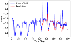
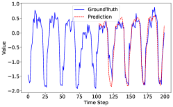
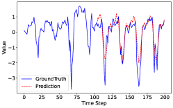
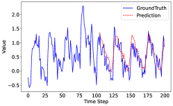
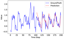
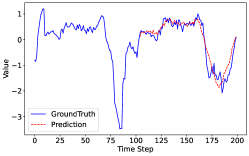
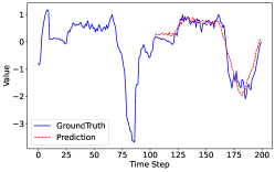
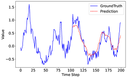
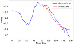
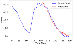
To clearly present the results, we select some representative samples for visualization analysis. Figure4 shows the long-term forecasting results from 4 different datasets. We select 3 typical forecasting results from 3 different dimensions of each datasets.


A.5 Imputation
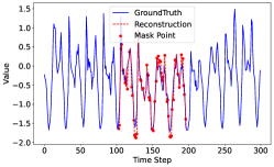
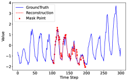
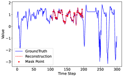
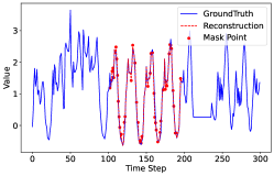
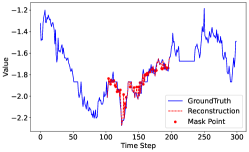
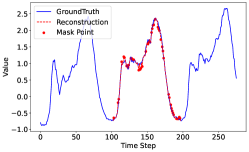
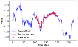
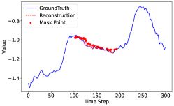
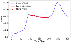
Figure5 illustrates the imputation results from three dimensions across four different datasets. Clearly, GTM can effectively reconstruct the missing data, adapting to varying data patterns.
A.5.1 Anomaly Detection
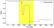
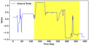
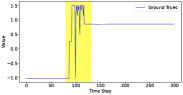
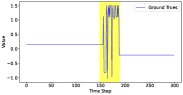
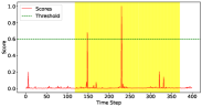
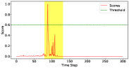
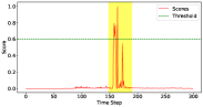
Figure 6 demonstrates four anomaly events detected by GTM in two datasets, along with their corresponding anomaly scores. The results align precisely with the labeled anomalies in the data.
A.6 Limitations and future work
So far, GTM has shown promising results in multi-task analysis of MTS, offering a novel approach to learning universal representations of MTS data. However, several challenges remain. Through a comprehensive survey of time series analysis models, we identified a significant issue beyond the scope of universal knowledge learning: the absence of unified benchmarks. Current models are often pre-trained on different datasets and employ varied hyperparameter settings, or involve complex processes to optimize performance. Consequently, researchers are left with two primary options for comparison: citing the best results from previous papers or attempting to reproduce these results under new conditions. However, due to time and resource constraints, build a framework for fair comparisons is challenging. Establishing a standardized, unified benchmark would be immensely beneficial for future research in this field.
Additionally, with adequate resources, further development of the GTM model, from employing a few low-rank knowledge attention modules to constructing extensive mixtures of experts (MoE) architectures, could significantly enhance its knowledge learning capabilities. This evolution could lead to more robust and versatile models, capable of addressing the diverse needs of MTS analysis.