Model Reference-Based Control with Guaranteed Predefined Performance for Uncertain Strict-Feedback Systems

Abstract

To address the complexities posed by time- and state-varying uncertainties and the computation of analytic derivatives in strict-feedback form (SFF) systems, this study introduces a novel model reference-based control (MRBC) framework which applies locally to each subsystem ($SS$), to ensure output tracking performance within the specified transient and steady-state response criteria. This framework includes 1) novel homogeneous adaptive estimators (HAEs) designed to match the uncertain nonlinear SFF system to a reference model, enabling easier analysis and control design at the $SS$ level, and 2) model-based homogeneous adaptive controllers enhanced by logarithmic barrier Lyapunov functions (HAC-BLFs), intended to control the reference model provided by HAEs in each $SS$, while ensuring the prescribed tracking responses under control amplitude saturation. The inherently robust MRBC achieves uniformly exponential stability using a generic stability connector term, which addresses dynamic interactions between the adjacent $SS$s. The parameter sensitivities of HAEs and HAC-BLFs in the MRBC framework are analyzed, focusing on the system’s robustness and responsiveness. The proposed MRBC framework is experimentally validated through several scenarios involving an electromechanical linear actuator system with an uncertain SFF, subjected loading disturbance forces challenging $0-95\%$ of its capacity.

I Introduction

A strict-feedback form (SFF) system, a class of uncertain nonlinear systems, garnered significant focus from 1990s in the realm of recursive control strategies [1] as they encompass a wide range of practical applications, including robot manipulators [2], electromechanical linear actuators (EMLAs) [3], and DC-DC buck converters [4]. In SSF systems, the hierarchical influence of control inputs on state dynamics renders each level dependent on preceding control actions. Therefore, they require control approaches to counteract the potential for finite escape instabilities inherent in an open loop [5]. Generally, for a system dynamics expressed as $x=f(x)+g(x)u$, the functional term $g(x)$ multiplied by the control input is the control gain function, the sign of which is referred to as the control direction [6, 7]. In certain SFF systems, the control gain is predetermined [8, 9, 10, 11], or its sign is known [12, 13, 14, 15, 16]. However, gaining a prior understanding of the control direction under broader conditions seems impractical [17]. To address unknown control directions in SFF systems, [6] introduced a group of error transformation functions. In addition, the modeling term $f(x)$ is considered to be definitively accurate and fully known in the SFF structure, as assumed in [9], or partially known, as assumed in [11]. Hence, [12] proposed a group of new feedback mechanisms to compensate for the unknown system dynamics.

In addition to these conservative assumptions in designing control for SFF systems, significant computational complexities, referred to as the “explosion of complexity,” have been noted [11, 18, 8, 6], stemming from the excessive growth of analytic derivatives in control designs due to the inherent recursiveness of these systems. To address this, [11] proposed a specific feedforward (FF) compensation term for each subsystem ($SS$) of a class of SFF systems, based on the system’s inverse dynamics. Similarly, command filters were employed in [19] and [20], to overcome the computational complexity and control singularity caused by the repeated derivation of virtual control functions in backstepping control applied to SFF systems.

Furthermore, most practical systems typically function within various input $u(t)$ and output $x(t)$ constraints, which may be due to physical limitations, performance requirements, or security considerations [13]. For example, system input amplitude saturation is common in SFF applications and can significantly degrade performance, potentially leading to system instability [21]. Hence, [22] proposed a state observer combined with a backstepping recursive approach to ensure the global boundedness of the closed-loop system with high probability. While recent successes have been reported, the challenges related to different types of uncertainties, including external disturbances, modeling and parametric uncertainties, and unknown control gains, affecting tracking control performance, remain inadequately addressed. Some novel control strategies, such as prescribed performance control (PPC), were recently explored in [15] and [16] to enhance both transient and steady-state performances while decreasing the computational burden of the control strategy. However, these schemes required the control direction to be known in advance. This problem was address in [14] through the introduction of smooth orientation functions. However, this study overlooked the control input peaking and amplitude saturation phenomenon.

Inspired by the aforementioned insights and building upon [6], [11], [23], and [24], this paper proposes a model reference-based control (MRBC) framework for a class of uncertain SFF systems. This framework has two functional stages:

I-1 Homogeneous adaptive estimators (HAEs)

As specific FF compensation terms, they are designed to transform an uncertain nonlinear SFF system into a certain reference model. The modeling terms of the reference system at the $SS$ levels are adaptively estimated, while the reference system states are matched to the uncertain nonlinear SFF system states of equivalent order.

I-2 Homogeneous adaptive controllers enhanced by logarithmic barrier Lyapunov functions (HAC-BLFs)

As FF compensation terms for the certain reference model obtained in the first stage, they are designed to actively engage based on the system’s inverse dynamics, generating the control input signal $u(t)$ from the reference system states and desired output, thereby enforcing the entire system to adhere to the prescribed tracking control responses at the $SS$ levels.

The schematic of the proposed MRBC framework is illustrated in Fig. 1.

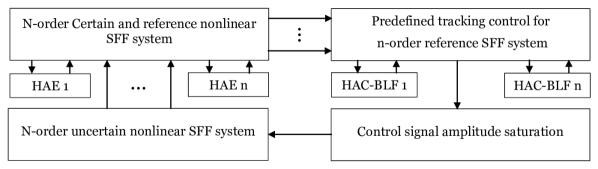
Figure 1: Schematic of the MRBC framework for an $n$-order SFF system.

The comparative contributions are as follows:

1) This paper considers a class of uncertain SFF systems that is subject to an unknown control gain function and its sign (contrary to [8, 9, 10, 11, 12, 13, 14, 15, 16]), time-varying disturbances, and state-dependent modeling uncertainties (contrary to [8, 9, 11]). As a systematic solution, HAEs transform the uncertain SFF system into a more user-friendly format for easier analysis and control design.

2) Unlike [6], which used mathematical manipulations due to the transformation of asymmetric constraints into symmetric forms of predefined tracking performance, HAC-BLFs guarantee tracking performance within the user-defined transient and steady-state performance by directly constraining the error symmetry form.

3) Built on [11] to address the challenges of computing analytic derivatives of virtual controls used in each $i$th subsystem ($SS_{i}$), where $i=1,\ldots,n$, of an $n$-order SSF system, this study eliminates the need for using analytic derivatives of virtual control (contrary to [8]). This is achieved by designing an MRBC framework based on the system inverse dynamics to generate the control input from the states and desired output of the system.

4) This paper extends the stability connector concept proposed in [11], where each SS with a “stability-preventing” connector is compensated by the subsequent SS with a corresponding “stabilizing” connector to achieve asymptotic stability. By employing the MRBC framework, the tracking error of the SSF system uniformly and exponentially converges to a stable region, whose radius depends on the intensity of the uncertainties. Built on [24], the parameter sensitivities of the MRBC framework are analyzed, with a focus on the trade-off between system responsiveness and uncertainty rejection.

The rest of this paper is organized as follows. Section II designs HAEs. Section III formulates HAC-BLFs. Section IV analyzes the control stability. Section V experimentally validates the proposed framework in a practical SFF system, an EMLA system. Finally, Section VI concludes this paper.

II Designing HAEs for an Uncertain Sff System

II-A Model Problem

Let us define $x_{i}\in\mathbb{R}$, where $i=1,\ldots,n$, as the system states and $\bm{x}_{i}=\left[x_{1},\ldots,x_{i}\right]^{T}\in\mathbb{R}^{i}$, $\bm{x}_{n}=\bm{x}\in\mathbb{R}^{n}$, and $u\in\mathbb{R}$ as the system input. As used in [9], an ideal $n$-order SSF system, especially suitable for model-based control approaches, can be represented as follows:

$$\small\left\{\begin{aligned} &\dot{x}_{i}(t)=x_{i+1}(t)+f_{i}\left(\boldsymbol{x}_{i},t\right)\\ &\dot{x}_{n}(t)=u(t)+f_{n}\left(\boldsymbol{x}_{n},t\right)\end{aligned}\right.$$ (1)

where the time- and state-variant functions $f_{i}:\mathbb{R}^{i}\times\mathbb{R}_{+}\rightarrow\mathbb{R}$ are known as modeling terms with a triangular structure [25]. However, the system representation (1) for many control applications, such as that in [11] and [26], is impractical. Based on [27], we address a class of SFF system representations by considering different systematic uncertainties:

$$\small\left\{\begin{aligned} &\dot{x}_{i}(t)=g_{i}\left(\boldsymbol{x}_{i},t\right)x_{i+1}(t)+f_{i}\left(\boldsymbol{x}_{i},t\right)+d_{i}\left(\bm{x}_{i},t\right)+\Gamma_{i}(t)\\ &\dot{x}_{n}(t)=g_{n}\left(\boldsymbol{x}_{n},t\right)u(t)+f_{n}\left(\boldsymbol{x}_{n},t\right)+d_{n}\left(\bm{x}_{n},t\right)+\Gamma_{n}(t)\end{aligned}\right.$$ (2)

where the time-variant function $\Gamma_{i}:\mathbb{R}_{+}\rightarrow\mathbb{R}$ is unknown external disturbance. The time- and state-variant functions $d_{i}:\mathbb{R}^{i}\times\mathbb{R}_{+}\rightarrow\mathbb{R}$ and $g_{i}\left(\bm{x}_{i},t\right):\mathbb{R}^{i}\times\mathbb{R}_{+}\rightarrow\mathbb{R}$ are triangular modeling errors and the functional control gain, respectively, both being sufficiently smooth and unknown. The time- and state-variant triangular modeling functions $f_{i}:\mathbb{R}^{n}\times\mathbb{R}_{+}\rightarrow\mathbb{R}$ are known and globally Lipschitz.

II-B Transformation of an Uncertain into a Certain SFF System Model

Hereinafter, for brevity, we frequently omit the notations $t$ and $\bm{x}_{i}$ from equations. We define a reference model based on the ideal one (1), as

$$\small\left\{\begin{aligned} &\dot{\hat{x}}_{i}=\hat{x}_{i+1}+f^{*}_{i}\\ &\dot{\hat{x}}_{n}=u+f^{*}_{n}\end{aligned}\right.$$ (3)

where $f^{*}_{i}:\mathbb{R}^{i}\times\mathbb{R}_{+}\rightarrow\mathbb{R}$ are modeling terms of the reference system at the $SS$ levels and can be defined based on adaptation errors $\tilde{\Psi}_{i}$ and estimation errors $e_{i}=x_{i}-\hat{x}_{i}$:

$$f^{*}_{i} =f_{i}+\xi_{i}\tilde{\Psi}_{i}e_{i}+\frac{1}{2}\lambda_{i}e_{i}+e_{i-1}$$ (4)

where $e_{0}=0$ and $\xi_{i}$ are positive constants. Homogenous terms $\xi_{i}\tilde{\Psi}_{i}e_{i}+\frac{1}{2}\lambda_{i}e_{i}+e_{i-1}$ play estimator roles to match the reference system states to the uncertain nonlinear SFF system states (2) with equivalent order. Adaptive laws $\tilde{\Psi}_{i}$ for each $SS_{i}$ are defined as:

$$\dot{\tilde{\Psi}}_{i}=-\beta_{i}\tilde{\Psi}_{i}+\xi_{i}e_{i}^{2}$$ (5)

where $\beta_{i}$ is a positive constant. Now, from the definition of $e_{i}$ as well as (3) and (4), we have:

$$\dot{e}_{i}=e_{i+1}+d^{*}_{i}+\Gamma_{i}-\xi_{i}\tilde{\Psi}_{i}e_{i}-\frac{1}{2}\lambda_{i}e_{i}-e_{i-1}$$ (6)

$$\dot{e}_{n}=d^{*}_{n}+\Gamma_{n}-\xi_{n}\tilde{\Psi}_{n}e_{n}-\frac{1}{2}\lambda_{n}e_{n}-e_{n-1}$$

where

$$d^{*}_{i}(\bm{x}_{i+1},t)=d_{i}(\bm{x}_{i},t)+(g_{i}\left(\bm{x}_{i},t\right)-1)x_{i+1}$$ (7)

Note that in some applications, like [28], $g_{i}(\bm{x}_{i},t)$ are known and equal to one. In the mentioned applications $d^{*}_{i}(\bm{x}_{i},t)=d_{i}(\bm{x}_{i},t)$; otherwise, based on [29] and [30], $d^{*}_{i}(\bm{x}_{i+1},t)$ will be non-triangular structures of uncertainties.

Remark II.1: It is commonly assumed that 1) the upper limit of disturbances $|\Gamma_{i}|$ is bounded and already known [31, 32]; 2) the partial knowledge of the $d_{i}(x_{i},t)$ function or its corresponding bounding functions are predefined [33, 31, 28]; 3) the bound of $g_{i}$ is known [34], or at least $g_{i}(\cdot)$, where $i=1,\ldots,n$, must follow a structure where it consists of an unknown constant multiplied by a known function [35]. Apart from the following assumption, this work requires no additional information about the system’s nonlinearities.

Assumption II.1: Following Remark II.2, we can assume that the functional control gain $g_{i}(\bm{x}_{i},t)$, modeling error and uncertainties $d_{i}(\bm{x}_{i},t)$, and external disturbances $\Gamma_{i}(t)$ are bounded (see [36, 37, 35, 32, 33, 31, 28]). This means that for all values of $x_{i}$ in its domain and for all times $t$, $|g_{i}(\bm{x}_{i},t)|$, $\left|d_{i}\left(\bm{x}_{i},t\right)\right|$, and $|\Gamma_{i}(t)|$ can always be bounded from above by positive functions and not grow infinitely large. This assumption is significant because it allows control strategies to address uncertainties without requiring infinite control effort. Since we will later in Section III demonstrate that the input signal $u$ and states are constrained within a defined and bounded value, as well as based on [6], we can assume that the unknown nonlinear functions $d^{*}_{i}=d_{i}+(g_{i}-1)x_{i+1}$ and $d^{*}_{n}=d_{n}+(g_{n}-1)u$ are also bounded.

II-C Stability of HAEs

Motivated by a key concept in the stability connector proposed in [11] and the virtual power flow proposed in [38], for system (2) with reference system (3) and HAEs provided in (4), new stability connectors are defined as

$$s_{i}=e_{i}e_{i+1}$$ (8)

Next, we will use this auxiliary function for the convergence analysis of Theorem II.1 in Appendix A.

Theorem II.1: Let us define a quadratic function as

$$V_{\text{ob }} =\sum_{i=1}^{n}\frac{1}{2}\hskip 2.84544pt[{e^{2}_{i}}+\tilde{\Psi}_{i}^{2}]$$ (9)

Employing (4) and (5) ensures the vector of the matching errors $\bm{e}_{ob}=\left[e_{1},\ldots,e_{n}\right]^{T}$ to be

$$\|\bm{e_{ob}}\|\leq\sqrt{{2V_{ob}\left(t_{0}\right)}}e^{-\frac{\rho_{ob}}{2}(t-t_{0})}+\sqrt{{2\ell_{ob}\rho_{ob}^{-1}}}$$ (10)

where $t_{0}$ is the initial time, $\rho_{ob}$ is a positive parameter that depends on the design parameters of the HAEs ($\lambda_{i}$ and $\beta_{i}$), and $\ell_{ob}$ is a positive parameter that depends on the intensity of the uncertainties $d_{i}^{*}$ and $\Gamma_{i}$.

Proof: See Appendix A and Section II.D.

II-D Parameter Sensitivity Analysis

Equation (10) that expresses $\|\bm{e_{ob}}\|$ converges uniformly and exponentially with the decay rate $\frac{\rho_{ob}}{2}$ within a stable region of radius $\sqrt{{2\ell_{ob}\rho_{ob}^{-1}}}$ (see Fig. 2).

Figure 2: Stable region for HAEs.

As discussed in [39], a trade-off exists between real-time responsiveness and the robustness capability of the system. This trade-off can be investigated as follows:

II-D1 Real-time responsiveness

includes the distance of the initial error from the stable region, and the convergence rate into the stable region.

II-D2 Robustness capability

includes uncertainty-rejecting capability, signifying the stable region radius.

The HAEs provided in (4) for each $SS_{i}$ require three positive parameters to be selected: $\xi_{i}$, $\beta_{i}$, and $\lambda_{i}$. In Fig. 2, we have three positive parameters forming the stable region–$V_{ob}(t_{0})$, $\ell_{ob}$, and $\rho_{ob}$–which are directly affected by the parameters of HAEs, which are shown in Table I, addressing the relevant equations. For further information, see Appendix A.

TABLE I: Parameter Setting Of Haes In Terms Of Responsiveness And Robustness.

HAEs’ design	Affected	Increase	Decrease
parameters	parameters	parameter	parameter
$\xi_{i}$	None	insensitive	insensitive
$\min_{i=1}^{n}\left\{\lambda_{i}-\delta_{i}-\zeta_{i},\hskip 2.84544pt2\beta_{i}\right\}$	$\rho_{ob}\text{in \eqref{53}}$	higher response	more robust

For the control parameter $\xi_{i}$, being positive is sufficient for system stability, and varying it does not affect the control performance. Although the arbitrary parameters $\zeta_{i}$ and $\delta_{i}$ are not design parameters of HAEs and their increase reduces the radius of the stable region, $\lambda_{i}$ must also be increased to ensure that $\rho_{ob}>0$. Thus, depending on the applications, demands, and intensity of systematic uncertainties, the trade-off between real-time responsiveness and robustness capability, based on Table I, should be considered.

III Designing Hac-Blfs For Tracking Control

III-A Control Input Amplitude Saturation

After discussing the reference model transformation in Section II, as indicated in Assumption II.1, we must apply a constraint on the system input signal $u(t)$. In this regard, an amplitude saturation function $\alpha(u(t))$ is employed, providing ${u}_{min}\leq u\leq{u}_{max}$, where $u_{min}$ and $u_{max}$ are defined as the lower and upper bounds, respectively. We can mathematically describe this saturation function, as $\alpha\left(u(t)\right)=\alpha_{1}u(t)+\alpha_{2}$, where

$$\alpha_{1}=\begin{cases}\frac{1}{\left|u\right|+1},&u\geq{u}_{max}\hskip 2.84544pt\text{or }\hskip 2.84544ptu\leq{u}_{min}\\ 1&{u}_{min}\leq u\leq{u}_{max}\end{cases}$$ (11)

$$\alpha_{2}=\begin{cases}{u}_{max}-\frac{u}{\left|u\right|+1},&u\geq{u}_{max}\\ 0&{u}_{min}\leq u\leq{u}_{max}\\ {u}_{min}-\frac{u}{\left|u\right|+1}&u\leq{u}_{min}\end{cases}$$

We define $\Delta_{u}=\alpha(u)-u=(\alpha_{1}-1)u+\alpha_{2}$, representing the intensity of saturation of the control input compared to the constraint one. Employing the control saturation function $\alpha(.)$, from (3), we have

$$\small\left\{\begin{aligned} &\dot{\hat{x}}_{i}=\hat{x}_{i+1}+f^{*}_{i}\\ &\dot{\hat{x}}_{n}=\alpha(u)+f^{*}_{n}\end{aligned}\right.$$ (12)

III-B Inverse Dynamic Control

We define tracking errors as $\bar{e}_{i}(t)=\hat{x}_{i}(t)-x_{id}(t)$, where $x_{1d}$ represents the bounded and differentiable reference trajectories for $SS_{1}$ within the domain $-\eta_{1}\leq x_{1d}\leq\eta_{1}$ and $\eta_{1}$ is a positive constant. Building on [11], and based on the system’s inverse dynamics for the reference SFF system in (3) which employs FF compensation $\bar{f}_{i}$, $x_{id}$ for $i=2,\ldots,n$ and, control input signal $u(t)$ are defined as follows:

$$\small\left\{\begin{aligned} &{{x}}_{(i+1)d}=\dot{x}_{id}+\bar{f}_{i}-f^{*}_{i}\\ &u=\dot{{x}}_{nd}+\bar{f}_{n}-f^{*}_{n}\end{aligned}\right.$$ (13)

where we propose FF compensation terms for each $SS_{i}$, as:

$$\bar{f}_{i}= -\frac{1}{2}\gamma_{i}\bar{e}_{i}-\epsilon_{i}\tilde{\theta}_{i}\frac{\bar{e}_{i}}{Q_{i}}-\frac{Q_{i}}{Q_{i-1}}\bar{e}_{i-1}$$ (14)

where $\epsilon_{i}$, and $\gamma_{i}$ are positive constants. $Q_{i}$ is a positive notation, and $\bar{e}_{0}=0$. $\tilde{\theta}_{i}$ are adaptive laws and can be defined as:

$$\dot{\tilde{\theta}}_{i}=-\kappa_{i}\tilde{\theta}_{i}+\epsilon_{i}(\frac{\bar{e}_{i}}{Q_{i}})^{2}$$ (15)

where $\kappa_{i}$ is a positive constant.

From (12) and (LABEL:14), we can obtain

$$\small\left\{\begin{aligned} \dot{\bar{e}}_{i}=&\dot{\hat{x}}_{i}-\dot{x}_{id}=\hat{x}_{i+1}+f^{*}_{i}-x_{(i+1)d}+\bar{f}_{i}-f^{*}_{i}\\ \dot{\bar{e}}_{n}=&\dot{\hat{x}}_{n}-\dot{x}_{nd}=\alpha(u)+f^{*}_{n}-u+\bar{f}_{n}-f^{*}_{n}\end{aligned}\right.$$ (16)

Therefore, we obtain

$$\small\left\{\begin{aligned} &\dot{\bar{e}}_{i}=\bar{e}_{i+1}+\bar{f}_{i}\\ &\dot{\bar{e}}_{n}=\Delta_{u}+\bar{f}_{n}\end{aligned}\right.$$ (17)

As observed in (LABEL:19), $\Delta_{u}$ is the uncertainty of the reference system when the control input signal exceeds the limitation ${u}_{min}\leq u\leq{u}_{max}$.

III-C Prescribed Tracking Control Performance

In prescribed performance control (PPC), singularities are often used to create a constraint that forces the system’s state to stay within a desired range of behaviors. This is done by incorporating a barrier function or transformation in the control law, which makes it impossible for the state to approach undesirable values, like going outside a predefined boundary. Built on [6], the expected tracking performance for each $SS_{i}$ is predetermined by $-o_{i}(t)<\bar{e}_{i}<o_{i}(t)$, where

$$o_{i}=\left(o^{shoot}_{i}-o^{bound}_{i}\right)e^{-o_{i}^{*}t}+o^{bound}_{i}$$ (18)

with $o^{shoot}_{i}>o_{i}^{bound}>0$ and $o_{i}^{*}>0$. The overshoot of $\bar{e}_{i}$ is limited to a value smaller than $o^{shoot}_{i}$. The final bound and convergence rate of $\bar{e}_{i}$ are represented by $o^{bound}_{i}$ and $o_{i}^{*}$, respectively. The tracking error-bound $o_{i}$ should be larger than the bound of the desired reference $\eta_{i}$, where for each $SS_{i}$, we assume domain $-\eta_{i}\leq x_{id}\leq\eta_{i}$, and $\eta_{i}$ is a positive constant. Later in Section III-D, we will describe a conditional function of each $SS_{i}$ using the properties of $\log\left(\frac{o_{i}^{2}}{Q_{i}}\right)$, whose domain, according to the definition $Q_{i}=o_{i}^{2}-\bar{e}_{i}^{2}$, is restricted by the condition that the denominator $Q_{i}$ must be positive. By selecting $\bar{e}_{i}(t_{0})<o_{i}(t_{0})$, as $\bar{e}_{i}$ approaches $o_{i}$, the value inside the logarithm approaches infinity because the denominator approaches zero and the function would be singular and undefined due to a negative argument in the logarithm.

III-D Stability of HAC-BLFs

Motivated by a key concept in the stability connector proposed in [11] and the virtual power flow proposed in [38], for system (12) with the proposed control, new stability connectors are defined as

$$\bar{s}_{i}=\frac{e_{i}}{Q_{i}}e_{i+1}$$ (19)

Next, we will use this auxiliary function for the convergence analysis of Theorem III.1 in Appendix B.

Lemma III.1 [40]: For any positive constant $o_{i}$, and given that $Q_{i}=o^{2}_{i}-\bar{e}^{2}_{i}$, the following inequality holds for all $\bar{e}_{i}$ satisfying $\left|\bar{e}_{i}\right|<o_{i}$:

$$\log\left(\frac{o_{i}^{2}}{Q_{i}}\right)<\frac{\bar{e}_{i}^{2}}{Q_{i}}$$ (20)

Theorem III.1: Let us define a quadratic function as

$$\bar{V}_{{cont}} =\sum_{i=1}^{n}\frac{1}{2}\log\left(\frac{o_{i}^{2}}{Q_{i}}\right)+\frac{1}{2}\tilde{\theta}_{i}^{2}$$ (21)

Employing (14) and (15) ensures that the logarithmic tracking error function $\sum_{i=1}^{n}\log\left(\frac{o_{i}^{2}}{Q_{i}}\right)$ is

$$\sum_{i=1}^{n}\log\left(\frac{o_{i}^{2}}{Q_{i}}\right)\leq 2\bar{V}_{cont}\left(t_{0}\right)e^{-\left\{\bar{\rho}_{cont}\left({t-t_{0}}\right)\right\}}+2\hskip 2.84544pt{\bar{\ell}}\hskip 2.84544pt{\bar{\rho}_{cont}}^{-1}$$ (22)

where $\bar{\rho}_{cont}$ is a positive parameter that depends on the design parameters of HAC-BLFs ($\gamma_{i}$ and $\kappa_{i}$), and $\bar{\ell}$ is a positive parameter that depends on the intensity of the uncertainty due to the over-saturation control input $\Delta_{u}$.

Proof: See Appendix B and Section III.E.

III-E Parameter Sensitivity Analysis

Similar to Section II.D, the HAC-BLFs provided in (14) for each $SS_{i}$ require selecting three positive parameters: $\epsilon_{i}$, $\kappa_{i}$, and $\gamma_{i}$. In Fig. 3, we have three positive parameters forming the stable region: $\bar{V}_{cont}(t_{0})$, $\bar{\ell}$, and $\bar{\rho}_{cont}$–which are directly affected by HAC-BLF parameters shown in Table II, addressing the relevant equations. For further information, see Appendix B. Thus, depending on application demands, and the intensity of the over-saturation control signal, the trade-off between real-time responsiveness and robustness capability based on Table II should be considered. Note that, for $i=1,...,n-1$, $\upsilon_{i}$ is zero and for $i=n$, $\upsilon_{n}$ is an arbitrary positive parameter [see (61)].

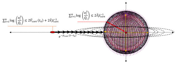
Figure 3: Stable region for HAC-BLFs.

TABLE II: Parameter setting of HAC-BLFs in terms of responsiveness and robustness.

HAEs’ design	Affected	Increase	Decrease
parameters	parameters	the parameter	the parameter
$\epsilon_{i}$	None	insensitive	insensitive
$\min_{i=1}^{n}\left\{\gamma_{i}-\upsilon_{i},\hskip 1.42271pt2\kappa_{i}\right\}$	$\bar{\rho}_{cont}\text{in \eqref{93}}$	higher response	more robust

IV Stability Of The MRBC Framework Including Haes And Hac-Blfs

Theorem IV.1: Let us define a quadratic function as

$$V_{all} =V_{ob}+\bar{V}_{cont}$$ (23)

$$=\sum_{i=1}^{n}\frac{1}{2}\hskip 2.84544pt[{e^{2}_{i}}+\tilde{\Psi}_{i}^{2}+\log\left(\frac{o_{i}^{2}}{Q_{i}}\right)+\tilde{\theta}_{i}^{2}]$$

Using the MRBC network, the accumulative error function $\sum_{i=1}^{n}e^{2}_{i}+\log\left(\frac{o_{i}^{2}}{Q_{i}}\right)$ for system (2), facing uncertainties $d_{i}$, $g_{i}$, and $\Gamma_{i}$, over-saturation control signal $\Delta_{u}$, and prescribed tracking control $-o_{i}<\bar{e}_{i}<o_{i}$ performance, converges uniformly and exponentially with the decay rate $\rho_{all}$, depending on the design parameters of MRBC ($\lambda_{i}$, $\gamma_{i}$, $\beta_{i}$, and $\kappa_{i}$), into a specific region centered at zero with radius $\ell_{all}$ depending on the intensity of the uncertainties.

Proof: See Appendix C.

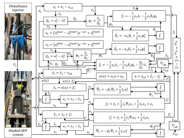
Figure 4: Schematic of the MRBC framework including HAEs and HAC-BLFs applied to the studied EMLA.

V Experimental Validity

The experiments were conducted by applying the MRBC framework including both HAEs and HAC-BLFs to a practical SFF system, an EMLA system equipped with a three-phase electric motor, gearbox, and ball screw in various scenarios. The motion dynamics of the system can be represented, based on [3], as follows:

$$\dot{v}_{L}=I^{-1}_{eq}\tau_{m}-I^{-1}_{eq}B_{eq}v_{L}-I^{-1}_{eq}K_{eq}x_{L}-I^{-1}_{eq}f_{eq}F_{L}$$ (24)

where $\tau_{m}$, $I_{eq},B_{eq},K_{eq}$, $f_{eq}$, and $F_{L}$ are the motor torque (measured in N.m), equivalent inertia (kg.m²), damping ($\frac{N.s}{m}$), spring effect ($\frac{N}{\mu.m}$), load coefficient of the actuator system, and load disturbance (N), respectively. By defining the position state ${x}_{L}$ (m) and velocity state $v_{L}$ ($\frac{m}{s}$) as $x_{1}$ and $x_{2}$, respectively, we have the following representation, based on (2):

$$\small\left\{\begin{aligned} &\dot{x}_{1}(t)=g_{1}\left(\boldsymbol{x}_{1},t\right)x_{2}(t)+f_{1}\left(\boldsymbol{x}_{1},t\right)+d_{1}\left(\bm{x}_{1},t\right)+\Gamma_{1}(t)\\ &\dot{x}_{2}(t)=g_{2}\left(\bm{x}_{2},t\right)u(t)+f_{2}\left(\boldsymbol{x}_{2},t\right)+d_{2}\left(\bm{x}_{2},t\right)+\Gamma_{2}(t)\end{aligned}\right.$$ (25)

where the modeling term for $SS_{1}$ is $f_{1}=0$. However, $g_{1}$, $d_{1}$, and $\Gamma_{1}$ are related to sensory noise and the derivatives effects of sensor data, causing undesired and nonlinear relationship between the derivative of position $\dot{x}_{1}$ and velocity $x_{2}$, for which we lacked specific information. Similarly, for $SS_{2}$, we have $u=\tau_{m}$, $g_{2}=I^{-1}_{eq}$, $f_{2}=-I^{-1}_{eq}K_{eq}x_{L}$, and $d_{2}=-I^{-1}_{eq}B_{eq}v_{L}$. Note that we assumed $g_{1,2}$, $d_{1,2}$, and $\Gamma_{1,2}$ to be unknown for the MRBC framework. We also employed another actuator at the load side of the experimented system, to generate functional loading force $F_{L}$, which introduced an unknown load disturbance, $\Gamma_{2}=-I^{-1}_{eq}f_{eq}F_{L}$, on the studied EMLA, varying its motor torque capacity by $0-95\%$. The setup under study, along with the MRBC framework, is shown in Fig.4. The control signals and communications between the setup components were managed via an EtherCAT network operated at a sampling rate of $1,000$ Hz. We defined 1) two set points at initial time $t_{0}$ as $x_{1d}(t_{0})=0.05$ m and $\dot{x}_{1d}(t_{0})=0$ m/s for the system sustainability under varying load disturbances and 2) trajectories (shown in Fig. 5) based on quintic polynomials from [41] for the system tracking under varying load disturbances. From (LABEL:14), we found the reference setpoint/trajectory of $SS_{1}$ as $x_{1d}$ and for $SS_{2}$ as ${{x}}_{2d}=\dot{x}_{1d}+\bar{f}_{1}-f^{*}_{1}$. The parameters of HAEs were set as $\lambda_{1,2}=500$, $\beta_{1,2}=0.8$, and $\xi_{1,2}=0.08$. The control parameters of HAC-BLFs were set as $\gamma_{1,2}=40$, $\epsilon_{1,2}=0.8$, and $\kappa_{1,2}=1$.

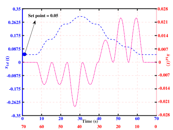
Figure 5: Reference Trajectory: $x_{1d}$ based on quantic polynomials [41] with set point $0.05$ and its derivative $\dot{x}_{1d}$.

For the MRBC-employed system, four experiments were conducted: 1) reaching and maintaining the system at the set point $x_{1d}=0.05$ m within the specific predefined control performance and under low-disturbance conditions (varying the motor capacity by up to $12.5\%$); 2) reaching and maintaining the system at the set point $x_{1d}=0.05$ m within the specific predefined control performance under high-disturbance conditions (varying of the the motor capacity by up to $92\%$); 3) maintaining the system to track the reference trajectory $x_{1d}$ based on meter shown in Fig. 5 within the specific predefined control performance under low-disturbance conditions (varying the motor capacity by up to $13\%$); and 4) maintaining the system to track the reference trajectory $x_{1d}$ shown in Fig. 5 within the specific predefined control performance under high-disturbance conditions, (varying the motor capacity by up to $95\%$).

V-A Experiment 1: Set Point Stabilization under Low-Disturbance Conditions (Load Force Varied by $0-12.5\%$ of the EMLA’s Capacity)

Regardless of the system’s initial point, we aimed to have the system reach and maintain the set point of $x_{1d}=0.05$, despite uncertainties in system and control directions ($d_{1,2}$ and $g_{1,2}$), as well as external disturbances ($\Gamma_{1,2}$). Based on Section II, and employing HAEs, we aimed to estimate $f^{*}_{1,2}$ and transform the uncertain system (25) into the certain model system (3), as follows:

$$\small\left\{\begin{aligned} \dot{\hat{x}}_{1}(t)&=\hat{x}_{2}(t)+f^{*}_{1}\left(x_{1},t\right)\\ \dot{\hat{x}}_{2}(t)&=u(t)+f^{*}_{2}\left(\bm{x}_{2},t\right)\end{aligned}\right.$$ (26)

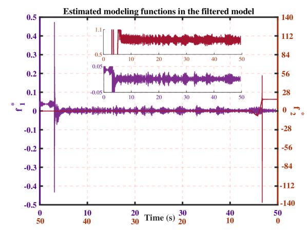
Figure 6: Experiment 1: The values of $f^{*}_{1,2}$ (measured in N.m) in estimated certain model (3) by employing HAEs.

Fig. 6 illustrates the estimated values of $f^{*}_{1}$ in purple and $f^{*}_{2}$ in dark red on two different scales (both measured in N.m) in the reference system. The errors between the new states of the reference model in (26) and the actual states of (25), are illustrated in Fig. 7 as $e_{1}=x_{1}-\hat{x}_{1}$ for $SS_{1}$ in blue and $e_{2}={x}_{2}-\hat{x}_{2}$ for $SS_{2}$ in red. The newly estimated states, $\hat{x}_{1}$ and $\hat{x}_{2}$, were obtained separately from the HAE’s input HAC-BLFs. To stabilize the states of the reference system $\hat{x}_{1}$ at the set point ($x_{1d}=0.05$), from (12), the reference trajectory for $SS_{2}$ based on the reference set point of $SS_{1}$ ($\dot{x}_{1d}=0$) as ${{x}}_{2d}=0+\bar{f}_{1}-f^{*}_{1}=\bar{f}_{1}-f^{*}_{1}$ was obtained. Similarly the control input signal was obtained as $u=\dot{{x}}_{2d}+\bar{f}_{2}-f^{*}_{2}$. Then, following (11) the control signal was constrained as $-19.5\leq u\leq 6$. The green trajectory in Fig. 8 illustrates the generated control signal, which adheres to the defined constraint. The orange trajectory in this figure also shows the external force $F_{L}$ applied to the EMLA (extracting $0-12.5\%$ of its capacity) to generate the low-disturbance term $\Gamma_{2}=-I^{-1}_{eq}f_{eq}F_{L}$ in this experiment. Based on (18), the expected control performance for $SS_{1}$ was defined as $o_{1}^{shoot}=0.1$, $o^{bound}_{1}=0.005$, and $o_{1}^{*}=0.0002$. Hence, Fig. 9 illustrates the control error for $SS_{1}$ by employing HAC-BLFs, adhering to the prescribed performance within $-o_{1}(t)<\bar{e}_{1}<o_{1}(t)$.

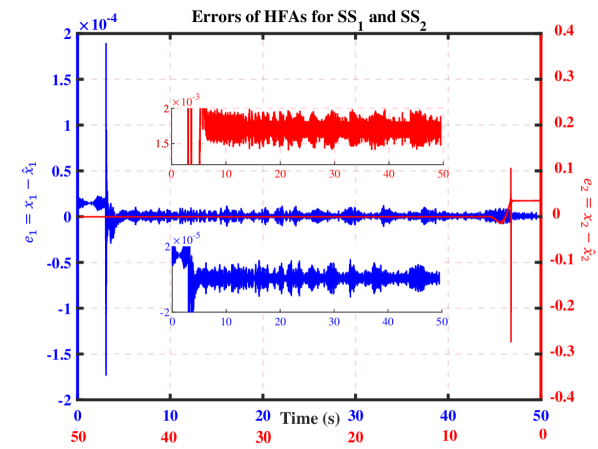
Figure 7: Experiment 1: The errors between new states of certain model (3) estimated by employing HAEs and states of the initial system form (2).

Figure 8: Experiment 1: The control signal constrained by the function $\alpha(.)$ and external force $F_{L}$ imposed on the system.

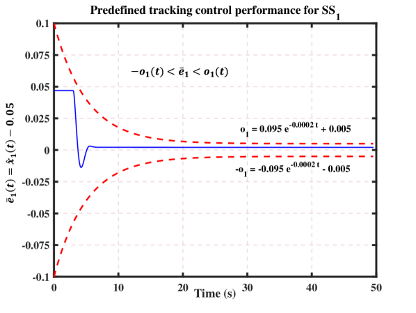
Figure 9: Experiment 1: Predefined set point-reaching performance of $SS_{1}$ by employing the HAC-BLF.

Similarly, the expected control performance for $SS_{2}$ was defined as $o_{2}^{shoot}=0.2$, $o^{bound}_{2}=0.005$, and $o_{2}^{*}=0.0002$. Hence, Fig. 10 illustrates the control error for $SS_{2}$ by employing HAC-BLFs, adhering to the prescribed performance within $-o_{2}(t)<\bar{e}_{2}<o_{2}(t)$.

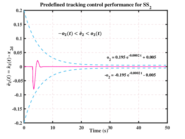
Figure 10: Experiment 1: Predefined control performance of $SS_{2}$ by employing the HAC-BLF.

V-B Experiment 2: Set Point Stabilization under High-Disturbance Conditions (Load Force Varied by $0-92\%$ of the EMLA’s capacity)

In this experiment similar to the previous one, regardless of the system’s initial point, we aimed to have the system reach and maintain the set point of $x_{1d}=0.05$ under the high-disturbance condition. Again, based on Section II, and employing HAEs, we aimed to estimate $f^{*}_{1,2}$ and transform the uncertain system (2) into the certain model system (3). As observed in Fig 11, gaining disturbance $\Gamma_{2}$ in $SS_{2}$ did not have a visible effect on $f^{*}_{1}$ (purple trajectory) relative to $SS_{1}$, while the estimation of $f^{*}_{2}$ (dark red trajectory) was impacted prominently.

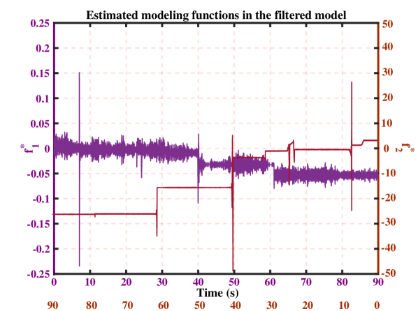
Figure 11: Experiment 2: The values of $f^{*}_{1,2}$ (measured in N.m) in certain model (3) estimated by employing HAEs.

Fig. 12 shows the errors between the new states of the reference model in (3), and the rough states of the initial system (2)($e_{1}=x_{1}-\hat{x}_{1}$ for $SS_{1}$ in blue and $e_{2}={x}_{2}-\hat{x}_{2}$ for $SS_{2}$ in red). Compared to experiment 1, the errors between the new states of the certain model in (3) and states of the initial form of system (2) under high-disturbance condition had a better transient but reduction in steady-state performance. The new estimated states $\hat{x}_{1}$ and $\hat{x}_{2}$ of the system were obtained separately from HAEs and input HAC-BLFs. To stabilize the states of the reference system $\hat{x}_{1}$ at the set point ($x_{1d}=0.05$), like experiment 1, ${{x}}_{2d}=0+\bar{f}_{1}-f^{*}_{1}=\bar{f}_{1}-f^{*}_{1}$ was obtained, and similarly, the control input signal was obtained as $u=\dot{{x}}_{2d}+\bar{f}_{2}-f^{*}_{2}$. Then, the control signal was constrained as $-2.5\leq u\leq 38$, following (11). As the external disturbance was loading force about $10$ times more intense compared to that in experiment 1, the value of the upper bound of control input $u_{max}$ was considered larger, while the lower bound $u_{min}$ was considered smaller.

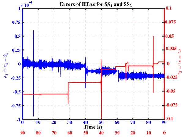
Figure 12: Experiment 2: The errors between new states of certain model (3) estimated by employing HAEs and states of the initial system form (2).

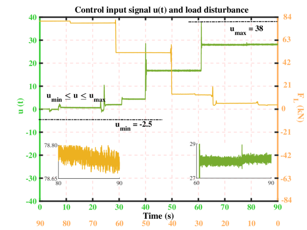
Figure 13: Experiment 2: The control signal constrained by the function $\alpha(.)$ and the external force $F_{L}$ imposed on the system.

The green trajectory in Fig. 13 illustrates the generated control signal, which adheres to the defined constraint while its amplitude increase to control the system under high-disturbance conditions. The orange trajectory in this figure also shows the external force $F_{L}$ applied to the EMLA (extracting $0-92\%$ of its capacity) to generate the external disturbance $\Gamma_{2}=-I^{-1}_{eq}f_{eq}F_{L}$.

In this scenario, based on (18), the expected control performance for $SS_{1}$ was defined as $o_{1}^{shoot}=0.005$, $o^{bound}_{1}=0.002$, and $o_{1}^{*}=0.0001$. Fig. 14 illustrates the control error incurred for $SS_{1}$ by employing HAC-BLFs, adhering to the prescribed performance within $-o_{1}(t)<\bar{e}_{1}<o_{1}(t)$.

Similarly, the expected control performance for $SS_{2}$ was defined as $o_{2}^{shoot}=0.150$, $o^{bound}_{2}=0.015$, and $o_{2}^{*}=0.0004$. Fig. 15 illustrates the control error incurred for $SS_{2}$ by employing HAC-BLFs, adhering to the prescribed performance within $-o_{2}(t)<\bar{e}_{2}<o_{2}(t)$.

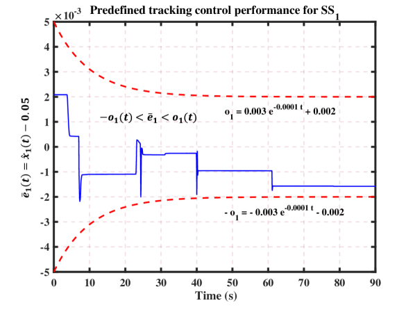
Figure 14: Experiment 2: Predefined set point-reaching performance of $SS_{1}$ by employing the HAC-BLF.

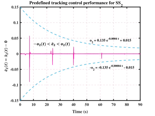
Figure 15: Experiment 2: Predefined control performance of $SS_{2}$ by employing the HAC-BLF.

V-C Experiment 3: Trajectory tracking under Low-Disturbance Conditions (Load Force Varied by $0-13\%$ of the EMLA’s Capacity)

In this experiment, regardless of the system’s initial point, we aimed to have it track the reference trajectory $x_{1d}$ shown in Fig. 5 under the low-disturbance conditions similar to the disturbance imposed on the system in experiment 1. Again, based on Section II, and employing HAEs, we aimed to estimate $f^{*}_{1,2}$ and transform the uncertain system (2) into the certain model system (3). As observed in Fig. 16, there is no prominent change in $f^{*}_{1}$ (purple trajectory) relative to $SS_{1}$. In contrast, the estimation of $f^{*}_{2}$ (dark red trajectory) was impacted prominently compared to experiment 1 because of the uncertain term $d_{2}=-I^{-1}_{eq}B_{eq}x_{2}$, generating more intense uncertainties by varying $x_{2}$, although $f^{*}_{2}$ was lower than that in experiment 2 facing high disturbance.

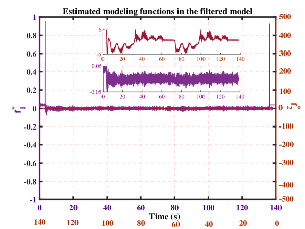
Figure 16: Experiment 3: The values of $f^{*}_{1,2}$ (measured in N.m) in certain model (3) estimated by employing HAEs.

Fig. 17 shows the errors between the new states of reference model (3), and the rough states of the initial system (2) ($e_{1}=x_{1}-\hat{x}_{1}$ for $SS_{1}$ in blue and $e_{2}={x}_{2}-\hat{x}_{2}$ for $SS_{2}$ in red). Compared to experiments 1 and 2, the error of state estimation in $SS_{1}$ was roughly similar, while that in $SS_{2}$ was worse than experiment 1 and better than experiment 2. The new estimated states $\hat{x}_{1}$ and $\hat{x}_{2}$ of the system were obtained from HAEs and input HAC-BLFs, separately.

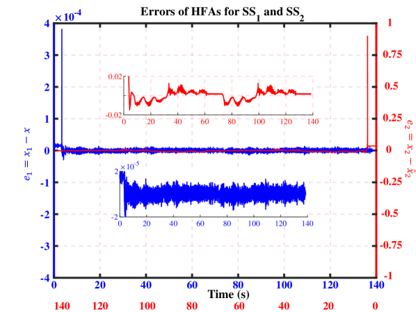
Figure 17: Experiment 3: The errors between new states of certain model in (3) estimated by employing HAEs and states of the initial system form (2).

We aimed for $\hat{x}_{1}$ to track the reference trajectory $x_{1d}$ shown in Fig.4. Based on (LABEL:14), the reference trajectory for $SS_{2}$ was obtained as ${{x}}_{2d}=\dot{x}_{1d}+\bar{f}_{1}-f^{*}_{1}$, and similarlym the control input signal was obtained as $u=\dot{{x}}_{2d}+\bar{f}_{2}-f^{*}_{2}$. Then, the control signal was constrained, as $-13\leq u\leq 6$, following (11).

The green trajectory in Fig. 18 illustrates the generated control signal, which adheres to the defined constraint. The orange trajectory in this figure also shows the external force $F_{L}$ applied to the EMLA (extracting $0-13\%$ of its capacity) to generate the external disturbance $\Gamma_{2}=-I^{-1}_{eq}f_{eq}F_{L}$ in this experiment.

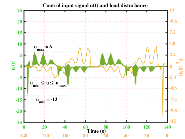
Figure 18: Experiment 3: The control signal constrained by the function $\alpha(.)$ and the external force $F_{L}$ imposed on the system.

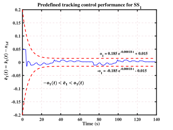
Figure 19: Experiment 3: Predefined control tracking performance of $SS_{1}$ by employing the HAC-BLF.

Based on (18), the expected control performance for $SS_{1}$ was defined as $o_{1}^{shoot}=0.2$, $o^{bound}_{1}=0.015$, and $o_{1}^{*}=0.00018$. Fig. 19 illustrates the control tracking error for $SS_{1}$ by employing HAC-BLFs, adhering to the prescribed performance within $-o_{1}(t)<\bar{e}_{1}<o_{1}(t)$.

Similarly, the expected control performance for $SS_{2}$ was defined as $o_{2}^{shoot}=0.2$, $o^{bound}_{2}=0.02$, and $o_{2}^{*}=0.0002$. Fig. 20 illustrates the control error for $SS_{2}$ by employing HAC-BLFs, adhering to the prescribed performance within $-o_{2}(t)<\bar{e}_{2}<o_{2}(t)$.

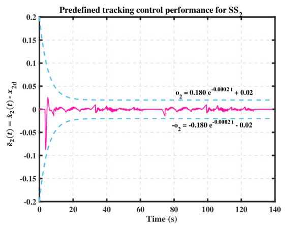
Figure 20: Experiment 3: Predefined control tracking performance of $SS_{2}$ by employing the HAC-BLF.

V-D Experiment 4: Trajectory tracking under High-Disturbance Conditions (load force variation $0-95\%$ of the capacity)

In this experiment, similar to experiment 3, regardless of the system’s initial point, we aimed to have it track the reference trajectory $x_{1d}$ shown in Fig.4; however, under the high-disturbance conditions, this setup caused sudden changes similar to the disturbance imposed on the system in experiment 2. We increased the controller sample time in this scenario and repeatedly varied the disturbance intensity, which could be beneficial for challenging the robustness of MRBC in tracking performance. Again, based on Section II, and employing HAEs, we aimed to estimate $f^{*}_{1,2}$ and transform the uncertain system (2) into certain model system (3).

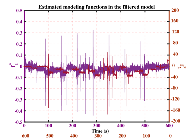
Figure 21: Experiment 4: The values of $f^{*}_{1,2}$ (measured in N.m) in certain model (3) estimated by employing HAEs.

As observed in Fig. 21, presenting severe disturbance with sudden changes in values yielded both estimated $f^{*}_{1}$ (purple trajectory) and $f^{*}_{2}$ (dark red trajectory). However, Fig. 22 shows the capability of HAEs to estimate states even under varying high-disturbance conditions and track for both $SS_{1}$ and $SS_{2}$.

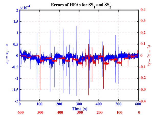
Figure 22: Experiment 4: The errors between new states of certain model in (3) estimated by employing HAEs and states of the initial system (2).

The new estimated states $\hat{x}_{1}$ and $\hat{x}_{2}$ of the system were obtained separately from HAEs and input HAC-BLFs. The aim was for these states to track the reference trajectories $x_{1d}$ and ${{x}}_{2d}=\dot{x}_{1d}+\bar{f}_{1}-f^{*}_{1}=\bar{f}_{1}-f^{*}_{1}$, shown Fig. 20. Similarly, the control input signal was obtained as $u=\dot{{x}}_{2d}+\bar{f}_{2}-f^{*}_{2}$. Then, the control signal was constrained, as $-15\leq u\leq 44.5$, following (11).

Note that, as the system tracked the references under the high-disturbance condition, the values of both upper and lower bound of the control input $u_{max}$ and $u_{min}$, were considered large (near the maximum of the motor torque capacity). The green trajectory in Fig.23 illustrates the generated control signal, which adheres to the defined constraint. The orange trajectory in this figure also shows the external force $F_{L}$ applied to the EMLA (extracting $0-95\%$ of its capacity) to generate the external disturbance $\Gamma_{2}=-I^{-1}_{eq}f_{eq}F_{L}$ in this experiment, which was about 20 times more intense than that in experiment 1, two times as intense as that in experiment 2, and four times as intense as that in experiment 3. In this scenario, the expected control performance for $SS_{1}$ was defined as $o_{1}^{shoot}=0.2$, $o^{bound}_{1}=0.015$, and $o_{1}^{*}=0.0001$. Fig. 24 illustrates the control error for $SS_{1}$ by employing HAC-BLFs, adhering to the prescribed performance within $-o_{1}(t)<\bar{e}_{1}<o_{1}(t)$. Similarly, the expected control performance for $SS_{2}$ was defined as $o_{2}^{shoot}=0.2$, $o^{bound}_{2}=0.09$, and $o_{2}^{*}=0.000008$. Fig. 25 illustrates the control error for $SS_{2}$ estimated by employing HAC-BLFs, adhering to the prescribed performance within $-o_{2}(t)<\bar{e}_{2}<o_{2}(t)$. Note that, due to sudden changes in disturbances, it was necessary to consider a wider predefined tracking performance for $SS_{2}$ that was directly affected by the external disturbance. This is evident in Fig. 25, where an exponential convergence rate of $0.000008$ was applied to the predefined performance.

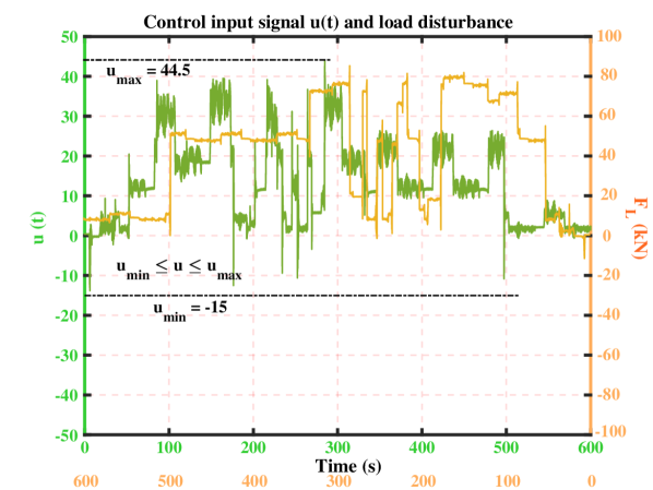
Figure 23: Experiment 4: The control signal constrained by the function $\alpha(.)$ and the external force $F_{L}$ imposed on the system.

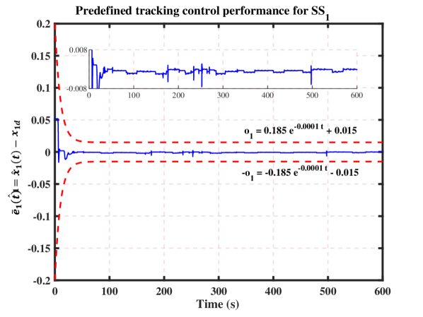
Figure 24: Experiment 4: Predefined control tracking performance of $SS_{1}$ by employing the HAC-BLF.

TABLE III: MRBC performance analysis in terms of responsiveness and rejecting uncertainty capability

Performance	$|F_{L}|\approx 1$	$|F_{L}|\approx 38$	$|F_{L}|\approx 9$	$|F_{L}|\approx 80$
criteria	Experiment 1 ($30\leq t\leq 50$)	Experiment 2 ($80\leq t\leq 90$)	Experiment 3 ($85\leq t\leq 90$)	Experiment 4 ($150\leq t\leq 175$)
$\sup|f^{*}_{1}|$	$1\times 10^{-2}$	$6\times 10^{-2}$	$4\times 10^{-2}$	$9\times 10^{-1}$
$\sup|f^{*}_{2}|$	$1$	$26$	$5.5$	$39$
$\sup|e_{1}|$	$1\times 10^{-5}$	$2.7\times 10^{-5}$	$1.8\times 10^{-5}$	$6\times 10^{-5}$
$\sup|e_{2}|$	$1.8\times 10^{-3}$	$5.2\times 10^{-2}$	$1\times 10^{-2}$	$6\times 10^{-2}$
$\sup|\alpha(u)|$	$0.4$	$28$	$6$	$40$
$\sup|\bar{e}_{1}|$	$1.1\times 10^{-4}$	$1.5\times 10^{-3}$	$1.4\times 10^{-3}$	$1.1\times 10^{-3}$
$\sup|\bar{e}_{2}|$	$1\times 10^{-4}$	$1\times 10^{-4}$	$2.5\times 10^{-4}$	$2.5\times 10^{-4}$

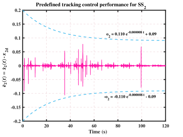
Figure 25: Experiment 4: Predefined control tracking performance of $SS_{2}$ by employing the HAC-BLF.

Table III presents a crucial analysis of MRBC performance, focusing on the trade-off between responsiveness and uncertainty rejection capabilities across different scenarios, as outlined in Sections I and II. For a clear analysis, we focused on data from a short period in each scenario under varying external disturbances. The table indicates that as uncertainties, including disturbances and control signal saturation, become more intense, the estimation errors for states in the certain model ($e_{1}$ and $e_{2}$) increase. Note that $f^{*}_{1}$ and $f^{*}_{2}$ represent uncertainty estimations in subsystems $SS_{1}$ and $SS_{2}$ of the initial SSF system and modeling terms in the reference SSF system, respectively. Larger disturbances resulted in higher control effort ($\alpha(u)$) amplitudes. Similarly, tracking errors in $SS_{1}$ in set point-reaching or tracking scenarios improved when the control efforts were lighter, likely due to the control amplitude saturation difference $\Delta_{u}$ affecting the accuracy of tracking control.

Interestingly, the tracking error in $SS_{2}$ remained similar regardless of the control efforts, although the set point-reaching scenarios demonstrated better accuracy compared to tracking scenarios, validating robustness and reliability of the proposed MRBC framework.

VI Conclusion

This paper proposed theoretical foundations, which were validated in practice, for controlling a class of $n$-order SFF systems including parametric and modeling uncertainties, unknown control gain functions, external disturbances, and control signal amplitude saturation effects. We presented auxiliary tools along with a specific stability connector, addressing dynamic interactions among the neighboring $SS$s, for a uniformly exponentially stable control while avoiding an excessive growth of the control design complexity and adhering to tracking responses within user-defined control performance. The proposed method included HAEs to convert an uncertain SFF system into a certain reference model and HAC-BLFs to guarantee tracking responses within a specified transient and steady-state response. Theoretical developments on uniformly exponential convergence (in Theorem IV.1) and adhering to the predefined tracking control performance were verified in experimental tests conducted on an EMLA with uncertain SFF subjected to external disturbances varying up to $95\%$ of the EMLA’s capacity. We left topics, such as control parameter optimizations, for future research.

Appendix A: Stability Proof For Haes

Proof of Theorem II.1: A quadratic function for $SS_{1}$ is suggested as follows:

$${V}_{1}=\frac{1}{2}\hskip 2.84544pt[{e^{2}_{1}}+\tilde{\Psi}_{1}^{2}]$$ (27)

From $\dot{e}_{1}$ and $\dot{\tilde{\Psi}}_{1}$ definitions in (LABEL:8) and (5) and knowing $e_{0}=0$, we have

$$\dot{V}_{1}= {e_{1}}e_{2}+{e_{1}}d^{*}_{1}+{e_{1}}\Gamma_{1}-\xi_{1}\tilde{\Psi}_{1}e^{2}_{1}-\frac{1}{2}\lambda_{1}e^{2}_{1}-\beta_{1}\tilde{\Psi}^{2}_{1}$$ (28)

$$+\xi_{1}e_{1}^{2}\tilde{\Psi}_{1}$$

From Assumption II.1 and using Young’s inequality and arbitrary positive constants $\delta_{1}$ and $\zeta_{1}$, we have:

$$\dot{V}_{1}\leq e_{1}e_{2}+\frac{\delta_{1}}{2}e_{1}^{2}+\frac{1}{2\delta_{1}}d_{1}^{*2}+\frac{\zeta_{1}}{2}e_{1}^{2}+\frac{1}{2\zeta_{1}}\Gamma_{1}^{2}-\frac{1}{2}\lambda_{1}e_{1}^{2}$$ (29)

$$-\beta_{1}\tilde{\Psi}_{1}^{2}$$

Therefore,

$$\dot{V}_{1}\leq e_{1}e_{2}-\frac{\lambda_{1}-\delta_{1}-\zeta_{1}}{2}e_{1}^{2}-\beta_{1}\tilde{\Psi}_{1}^{2}+\frac{1}{2\delta_{1}}d_{1}^{*2}+\frac{1}{2\zeta_{1}}\Gamma_{1}^{2}$$ (30)

Let us define:

$$\rho_{1}=\min[\lambda_{1}-\delta_{1}-\zeta_{1},\hskip 2.84544pt2\beta_{1}],\hskip 5.69046pt\ell_{1}=\frac{1}{2\delta_{1}}d_{1}^{*2}+\frac{1}{2\zeta_{1}}\Gamma_{1}^{2}$$ (31)

To guarantee $\rho_{1}>0$, we should select $\lambda_{1}$ large enough to satisfy $\lambda_{1}>\delta_{1}+\zeta_{1}$. Hence, from (8), (31), and (30),

$$\dot{V}_{1} \leq s_{1}-\rho_{1}V_{1}+\ell_{1}$$ (32)

Similarly, we can define quadratic functions for $SS_{i}$ for $i=2,\ldots,n-1$, as

$${V}_{i}=\frac{1}{2}\hskip 2.84544pt[{e^{2}_{i}}+\tilde{\Psi}_{i}^{2}]$$ (33)

and reaching

$$\dot{V}_{i}\leq {e_{i}}e_{i+1}-{e_{i}}e_{i-1}-\rho_{i}V_{i}+\ell_{i}$$ (34)

$$\leq s_{i}-s_{i-1}-\rho_{i}V_{i}-\rho_{i}V_{i}+\ell_{i}$$

where

$$\rho_{i}=\min[\lambda_{i}-\delta_{i}-\zeta_{i},\hskip 2.84544pt2\beta_{i}],\hskip 5.69046pt\ell_{i}=\frac{1}{2\delta_{i}}d_{i}^{*2}+\frac{1}{2\zeta_{i}}\Gamma_{i}^{2}$$ (35)

Finally, we can define a similar quadratic function for $SS_{n}$, as

$${V}_{n}=\frac{1}{2}\hskip 2.84544pt[{e^{2}_{n}}+\tilde{\Psi}_{n}^{2}]$$ (36)

and reaching

$$\dot{V}_{n}\leq -{e_{n}}e_{n-1}-\rho_{n}V_{n}+\ell_{n}$$ (37)

$$\leq -s_{n-1}-\rho_{n}V_{n}+\ell_{n}$$

where

$$\rho_{n}=\min[\lambda_{n}-\delta_{n}-\zeta_{n},\hskip 2.84544pt2\beta_{n}],\hskip 5.69046pt\ell_{n}=\frac{1}{2\delta_{n}}d_{n}^{*2}+\frac{1}{2\zeta_{n}}\Gamma_{n}^{2}$$ (38)

Now, we can define a quadratic function for the entire SSF system employing HAEs:

$$V_{\text{ob }} =V_{1}+\sum_{i=2}^{n-1}V_{i}+V_{n}=\frac{1}{2}(\bm{e}_{ob}^{\top}\bm{e}_{ob}+\bm{\Psi}^{\top}\bm{\Psi})$$ (39)

where $\bm{e}_{ob}=\left[e_{1},\ldots,e_{n}\right]^{T}$ and $\bm{\Psi}=\left[\tilde{\Psi}_{1},\ldots,\tilde{\Psi}_{n}\right]^{T}$. The derivative of (39), based on (32), (34), and (37), can be expressed as

$$\dot{V}_{ob}\leq\sum_{i=1}^{n-1}\left[-s_{i}+s_{i}\right]-\rho_{ob}V_{ob}+{\ell}_{ob}$$ (40)

where:

$$\rho_{ob}= \min[\rho_{1},...,\rho_{n}]=\min[\min_{i=1}^{n}\left\{\lambda_{i}-\delta_{i}-\zeta_{i},\hskip 2.84544pt2\beta_{i}\right\}]$$ (41)

$$\ell_{ob}= \ell_{1}+...+\ell_{n}=\sum_{i=1}^{n}\frac{1}{2\delta_{i}}d_{i}^{*2}+\frac{1}{2\zeta_{i}}\Gamma_{i}^{2}$$

As observed, term $e_{i+1}$ for $SS_{i}$ was treated as an external input that caused $s_{i}$ to appear in the $i$th $SS$. Hence, using the proposed HAEs (4), instability terms $s_{i}$ in each $SS$, provided in (8), were canceled out for the entire system’s stability. Thus, we have

$$\dot{V}_{ob}\leq-\rho_{ob}V_{ob}+{\ell}_{ob}$$ (42)

We can solve (42) as follows:

$$V_{ob}\leq V_{ob}\left(t_{0}\right)e^{-\left\{\rho_{ob}\left({t-t_{0}}\right)\right\}}+{\ell_{ob}}\int_{t_{0}}^{t}e^{\left\{-\rho_{ob}(t-T)\right\}}\hskip 5.69046ptdT$$ (43)

Because $e^{-\rho_{ob}(t-t_{0})}$ is always decreasing,

$$V_{ob}\leq V_{ob}\left(t_{0}\right)e^{-\left\{\rho_{ob}\left({t-t_{0}}\right)\right\}}+\hskip 2.84544pt{\ell_{ob}}\hskip 2.84544pt{\rho_{ob}}^{-1}$$ (44)

From (39), we can say:

$$\hskip-8.5359pt\|\bm{e}_{ob}\|^{2}\leq 2V_{ob}\left(t_{0}\right)e^{-\left\{\rho_{ob}\left({t-t_{0}}\right)\right\}}+2\hskip 2.84544pt{\ell_{ob}}\hskip 2.84544pt{\rho_{ob}}^{-1}$$ (45)

Based on Minkowski’s inequality, we reach:

$$\|\bm{e_{ob}}\|\leq\sqrt{{2V_{ob}\left(t_{0}\right)}}e^{-\frac{\rho_{ob}}{2}(t-t_{0})}+\sqrt{{2\ell_{ob}\rho_{ob}^{-1}}}$$ (46)

Thus, based on [42], it is clear from (46) that the vector of the estimation errors $\|\bm{e_{ob}}\|$ reaches a defined region $g_{0}\left({\tau}_{0}\right)$ in uniformly exponential convergence, such that

$$g_{0}\left({\tau}_{0}\right):=\left\{\|\bm{e_{ob}}\|\leq\bar{\tau}_{0}:=\sqrt{{2\ell_{ob}\rho_{ob}^{-1}}}\right\}$$ (47)

Appendix B: Stability Proof For Hac-Blfs

Proof of Theorem III.1: By using the proposed HAC-BLFs for each $SS_{i}$ in (14), we can define a quadratic function for $SS_{1}$, as [43]

$$\bar{V}_{1}=\frac{1}{2}\log\left(\frac{o_{1}^{2}}{Q_{1}}\right)+\frac{1}{2}\tilde{\theta}_{1}^{2}$$ (48)

As we can provide the initial estimated state $\hat{x}_{1}(t_{0})$ and the reference trajectory $x_{1d}(t_{0})$, we can select them to satisfy: $\bar{e}_{1}(t_{0})=\hat{x}_{1}(t_{0})-x_{1d}(t_{0})<o_{1}$; inserting (14) and (15), and knowing $\bar{e}_{0}=0$, we have

$$\dot{\bar{V}}_{1}= \frac{\bar{e}_{1}}{Q_{1}}\bar{e}_{2}-\frac{1}{2}\gamma_{1}\frac{\bar{e}_{1}}{Q_{1}}\bar{e}_{1}-\epsilon_{1}\tilde{{\theta}}_{1}(\frac{\bar{e}_{1}}{Q_{1}})^{2}+\epsilon_{1}\tilde{{\theta}}_{1}(\frac{\bar{e}_{1}}{Q_{1}})^{2}-\kappa_{1}\tilde{\theta}^{2}_{1}$$ (49)

Using Lemma III.1:

$$\dot{\bar{V}}_{1}\leq \frac{\bar{e}_{1}}{Q_{1}}\bar{e}_{2}-\frac{1}{2}\gamma_{1}\log\left(\frac{o_{1}^{2}}{Q_{1}}\right)-\kappa_{1}\tilde{\theta}^{2}_{1}$$ (50)

From (48) and (19), we obtain

$$\dot{\bar{V}}_{1}\leq \bar{s}_{1}-\bar{\rho}_{1}\bar{V}_{1},\hskip 5.69046pt\bar{\rho}_{1}=\min[\gamma_{1},\hskip 2.84544pt2\kappa_{1}],$$ (51)

Similarly, we can define quadratic functions for each $SS_{i}$ for $i=2,\ldots,n-1$, as

$$\bar{V}_{i}=\frac{1}{2}\log\left(\frac{o_{i}^{2}}{Q_{i}}\right)+\frac{1}{2}\tilde{\theta}_{i}^{2}$$ (52)

we have $\bar{e}_{i}(t_{0})<o_{i}$ and inserting (15) and (LABEL:19), we have

$$\dot{\bar{V}}_{i}= \frac{\bar{e}_{i}}{Q_{i}}\bar{e}_{i+1}\dot{\bar{e}}_{i}+\tilde{\theta}_{i}\dot{\tilde{\theta}}_{i}$$ (53)

$$= \frac{\bar{e}_{i}}{Q_{i}}\bar{e}_{i+1}-\frac{1}{2}\gamma_{i}\frac{\bar{e}_{i}}{Q_{i}}\bar{e}_{i}-\epsilon_{i}\tilde{\theta}_{i}(\frac{\bar{e}_{i}}{Q_{i}}\bar{e}_{i+1})^{2}$$

$$-\frac{\bar{e}_{i}}{Q_{i}}\frac{Q_{i}}{Q_{i-1}}\bar{e}_{i-1}-\kappa_{i}\tilde{\theta}^{2}_{i}+\epsilon_{i}\tilde{\theta}_{i}(\frac{\bar{e}_{i}}{Q_{i}}\bar{e}_{i+1})^{2}$$

Thus,

$$\dot{\bar{V}}_{i}= \frac{\bar{e}_{i}}{Q_{i}}\bar{e}_{i+1}-\frac{1}{2}\gamma_{i}\frac{\bar{e}^{2}_{i}}{Q_{i}}-\frac{\bar{e}_{i}}{Q_{i-1}}\bar{e}_{i-1}-\kappa_{i}\tilde{\theta}^{2}_{i}$$ (54)

Using Lemma III.1, and (19),

$$\dot{\bar{V}}_{i}= \bar{s}_{i}-\frac{1}{2}\gamma_{i}\log\left(\frac{o_{i}^{2}}{Q_{i}}\right)-\bar{s}_{i-1}-\kappa_{i}\tilde{\theta}^{2}_{i}$$ (55)

Therefore,

$$\dot{\bar{V}}_{i}\leq \bar{s}_{i}-\bar{\rho}_{i}\bar{V}_{i}-\bar{s}_{i-1}+\bar{\ell}_{i},\hskip 5.69046pt\bar{\rho}_{i}=\min[\gamma_{i},\hskip 2.84544pt2\kappa_{i}]$$ (56)

Similarly, we can define another quadratic function for $SS_{n}$, as

$$\bar{V}_{n}=\frac{1}{2}\log\left(\frac{o_{n}^{2}}{Q_{n}}\right)+\frac{1}{2}\tilde{\theta}_{n}^{2}$$ (57)

By selecting $\bar{e}_{n}(t_{0})<o_{n}$ and inserting (15) and (LABEL:19), we have

$$\dot{\bar{V}}_{n}= \frac{\bar{e}_{n}}{Q_{n}}\dot{\bar{e}}_{n}+\tilde{\theta}_{n}\dot{\tilde{\theta}}_{i}$$ (58)

$$= \frac{\bar{e}_{n}}{Q_{n}}\Delta_{u}-\frac{1}{2}\gamma_{n}\frac{\bar{e}_{n}}{Q_{n}}\bar{e}_{n}-\epsilon_{n}\tilde{\theta}_{n}(\frac{\bar{e}_{n}}{Q_{n}})^{2}$$

$$-\frac{\bar{e}_{n}}{Q_{n}}\frac{Q_{n}}{Q_{n-1}}\bar{e}_{n-1}-\kappa_{n}\tilde{\theta}^{2}_{n}+\epsilon_{n}\tilde{\theta}_{n}(\frac{\bar{e}_{n}}{Q_{n}})^{2}$$

By defining an unknown positive constant as $\alpha_{max}=|\Delta_{u}|$, we can say:

$$\dot{\bar{V}}_{n}\leq \frac{|\bar{e}_{n}|}{Q_{n}}\alpha_{max}-\frac{1}{2}\gamma_{n}\frac{\bar{e}^{2}_{n}}{Q_{n}}-\frac{\bar{e}_{n}}{Q_{n-1}}\bar{e}_{n-1}-\kappa_{n}\tilde{\theta}^{2}_{n}$$ (59)

Based on Young’s inequality and arbitrary positive constant $\upsilon_{n}$, and knowing that $Q_{n}$ is a positive notation, we have

$$\dot{\bar{V}}_{n}\leq \frac{\upsilon_{n}}{2}\frac{\bar{e}^{2}_{n}}{Q_{n}}+\frac{\alpha^{2}_{max}}{2\upsilon_{n}Q_{n}}-\frac{1}{2}\gamma_{n}\frac{\bar{e}^{2}_{n}}{Q_{n}}-\frac{\bar{e}_{n}}{Q_{n-1}}\bar{e}_{n-1}$$ (60)

$$-\kappa_{n}\tilde{\theta}^{2}_{n}$$

From (57) and (19), for any $\gamma_{n}>\upsilon_{n}$, we have

$$\dot{\bar{V}}_{n}\leq -\bar{s}_{n-1}-\bar{\rho}_{n}\bar{V}_{n}+\frac{\alpha^{2}_{max}}{2\upsilon_{n}Q_{n}},\hskip 2.84544pt\bar{\rho}_{n}=\min[\gamma_{n}-\upsilon_{n},\hskip 1.42271pt2\kappa_{n}]$$ (61)

Now, we can define a quadratic function for all proposed HAC-BLFs employed by the reference system (12), as

$$\bar{V}_{{cont}} =\sum_{i=1}^{n}\bar{V}_{i}=\sum_{i=1}^{n}\frac{1}{2}\log\left(\frac{o_{i}^{2}}{Q_{i}}\right)+\frac{1}{2}\tilde{\theta}_{i}^{2}$$ (62)

The derivative of (62), based on (51), (56), and (61), can be expressed as

$$\dot{\bar{V}}_{{cont}} \leq\sum_{i=1}^{n-1}\left[-\bar{s}_{i}+\bar{s}_{i}\right]-\bar{\rho}_{cont}\bar{V}_{cont}+\bar{\ell}$$ (63)

where

$$\bar{\rho}_{cont}= \min[\bar{\rho}_{1},...,\bar{\rho}_{n}]=\min[\min_{i=1}^{n}\left\{\gamma_{i},2\kappa_{i}\right\}]$$ (64)

$$\bar{\ell}= \frac{\alpha^{2}_{max}}{2\upsilon_{n}Q_{n}}$$

As observed, similar to (40), term $e_{i+1}$ for $SS_{i}$ is treated as an external input that causes $\bar{s}_{i}$ to appear in the $i$th SS. Hence, by using the proposed control (14), instability terms $\bar{s}_{i}$ in each $SS$, provided in (19), will be canceled out for the entire system. Thus, we have

$$\dot{\bar{V}}_{{cont}}\leq-\bar{\rho}_{cont}{\bar{V}}_{{cont}}+\bar{\ell}$$ (65)

We can solve (65), as follows:

$${\bar{V}}_{{cont}}\leq {\bar{V}}_{{cont}}\left(t_{0}\right)e^{-\left\{\bar{\rho}_{cont}\left({t-t_{0}}\right)\right\}}+\bar{\ell}\int_{t_{0}}^{t}e^{\left\{-\bar{\rho}_{cont}(t-T)\right\}}dT$$ (66)

Because $e^{-\bar{\rho}_{cont}(t-T)}$ is always decreasing,

$$\bar{V}_{cont}\leq \bar{V}_{cont}\left(t_{0}\right)e^{-\left\{\bar{\rho}_{cont}\left({t-t_{0}}\right)\right\}}+\hskip 2.84544pt\bar{\ell}\hskip 2.84544pt{\bar{\rho}_{cont}}^{-1}$$ (67)

From (62), we can say

$$\sum_{i=1}^{n}\log\left(\frac{o_{i}^{2}}{Q_{i}}\right)\leq 2\bar{V}_{cont}\left(t_{0}\right)e^{-\left\{\bar{\rho}_{cont}\left({t-t_{0}}\right)\right\}}+2\hskip 2.84544pt{\bar{\ell}}\hskip 2.84544pt{\bar{\rho}_{cont}}^{-1}$$ (68)

Thus, $\sum_{i=1}^{n}\log\left(\frac{o_{i}^{2}}{Q_{i}}\right)$ reaches a defined region $g_{1}\left({\tau}_{1}\right)$ in uniformly exponential convergence, such that

$$g_{1}\left({\tau}_{1}\right):=\left\{\sum_{i=1}^{n}\log\left(\frac{o_{i}^{2}}{Q_{i}}\right)\leq\bar{\tau}_{1}:={2\hskip 2.84544pt{\bar{\ell}}\hskip 2.84544pt{\bar{\rho}_{cont}}^{-1}}\right\}$$ (69)

Appendix C: Stability Proof For The MRBC Framework

Proof of Theorem IV.1: We can define a quadratic function for the uncertain system (2) employing HAEs and HAC-BLFs as

$$V_{all} =V_{ob}+\bar{V}_{cont}$$ (70)

$$=\sum_{i=1}^{n}\frac{1}{2}\hskip 2.84544pt[{e^{2}_{i}}+\tilde{\Psi}_{i}^{2}+\log\left(\frac{o_{i}^{2}}{Q_{i}}\right)+\tilde{\theta}_{i}^{2}]$$

Based on (40) and (63), we obtain

$$\dot{V}_{all}\leq-\rho_{ob}V_{ob}+{\ell}_{ob}-\bar{\rho}_{cont}\bar{V}_{cont}+\bar{\ell}$$ (71)

Straightforwardly, we can say

$$\dot{V}_{all}\leq-\rho_{all}V_{all}+{\ell}_{all}$$ (72)

where $\rho_{all}=\min[\rho_{ob},\bar{\rho}_{cont}]$ and $\ell_{all}=\ell_{ob}+\bar{\ell}$. We can solve (65) as follows:

$${{V}}_{{all}}\leq {{V}}_{{all}}\left(t_{0}\right)e^{-\left\{{\rho}_{all}\left({t-t_{0}}\right)\right\}}+{\ell}_{all}\int_{t_{0}}^{t}e^{\left\{-{\rho}_{all}(t-T)\right\}}dT$$ (73)

From (71), we can say:

$$\sum_{i=1}^{n}e^{2}_{i}+\log\left(\frac{o_{i}^{2}}{Q_{i}}\right)\leq 2V_{all}\left(t_{0}\right)e^{-{\rho_{all}(t-t_{0})}}+2\ell_{all}\rho_{all}^{-1}$$ (74)

Therefore, $\sum_{i=1}^{n}e^{2}_{i}+\log\left(\frac{o_{i}^{2}}{Q_{i}}\right)$ with initial time $t_{0}$ converging uniformly and exponentially within a specific region $g_{2}\left({\tau}_{2}\right)$ centered at zero such that

$$g_{2}\left({\tau}_{2}\right):=\left\{\sum_{i=1}^{n}e^{2}_{i}+\log\left(\frac{o_{i}^{2}}{Q_{i}}\right)\leq\bar{\tau}_{2}:=\sqrt{{2\hskip 2.84544pt{{\ell}_{all}}\hskip 2.84544pt{{\rho}_{all}}^{-1}}}\right\}$$ (75)

Mehdi Heydari Shahna earned a B.Sc. in electrical engineering from Razi University, Kermanshah, Iran, in 2015 and an M.Sc. in control engineering at Shahid Beheshti University, Tehran, Iran, in 2018. Since December 2022, he has been pursuing his doctoral degree in automation technology and mechanical engineering at Tampere University, Tampere, Finland. His research interests encompass robust control, robotics, fault-tolerant algorithms, and system stability.

Jukka-Pekka Humaloja received a Ph.D. in 2019 and worked as a postdoctoral research fellow until 2021 in the Systems Theory Research Group, Tampere University, Finland. During 2021–2023, he was a postdoctoral fellow in the Distributed Parameter System Lab at the University of Alberta, Canada. He is currently a postdoctoral researcher at the Technical University of Crete, Greece. His research interests include nonlinear control, adaptive control for distributed parameter systems, and advanced control strategies for complex systems.

Jouni Mattila received an M.Sc. and Ph.D. in automation engineering from Tampere University of Technology, Tampere, Finland, in 1995 and 2000, respectively. He is currently a professor of machine automation in the Automation Technology and Mechanical Engineering Unit at Tampere University. His research interests include machine automation, nonlinear-model-based control of robotic manipulators, and energy-efficient control of heavy-duty mobile manipulators.

References

- [1] Y. Li, Y.-X. Li, and S. Tong, “Event-based finite-time control for nonlinear multiagent systems with asymptotic tracking,” IEEE Transactions on Automatic Control, vol. 68, no. 6, pp. 3790–3797, June 2022.
- [2] L. Xing, C. Wen, Z. Liu, H. Su, and J. Cai, “Event-triggered adaptive control for a class of uncertain nonlinear systems,” IEEE Transactions on Automatic Control, vol. 62, no. 4, pp. 2071–2076, April 2016.
- [3] M. Heydari Shahna, M. Bahari, and J. Mattila, “Robust decomposed system control for an electro-mechanical linear actuator mechanism under input constraints,” International Journal of Robust and Nonlinear Control, vol. 34, no. 7, pp. 4440–4470, January 2024.
- [4] C. Zhang, J. Wang, S. Li, B. Wu, and C. Qian, “Robust control for pwm-based dc–dc buck power converters with uncertainty via sampled-data output feedback,” IEEE Transactions on Power Electronics, vol. 30, no. 1, pp. 504–515, January 2014.
- [5] M. Krstic, “Feedback linearizability and explicit integrator forwarding controllers for classes of feedforward systems,” IEEE Transactions on Automatic Control, vol. 49, no. 10, pp. 1668–1682, October 2004.
- [6] J.-X. Zhang and G.-H. Yang, “Low-complexity tracking control of strict-feedback systems with unknown control directions,” IEEE Transactions on Automatic Control, vol. 64, no. 12, pp. 5175–5182, December 2019.
- [7] L. Li, K. Zhao, Z. Zhang, and Y. Song, “Dual-channel event-triggered robust adaptive control of strict-feedback system with flexible prescribed performance,” IEEE Transactions on Automatic Control, vol. 69, no. 3, pp. 1752–1759, October 2023.
- [8] B. Liu, M. Hou, C. Wu, W. Wang, Z. Wu, and B. Huang, “Predefined-time backstepping control for a nonlinear strict-feedback system,” International Journal of Robust and Nonlinear Control, vol. 31, no. 8, pp. 3354–3372, February 2021.
- [9] L. Zhang, C. Deng, and L. An, “Asymptotic tracking control of nonlinear strict-feedback systems with state/output triggering: A homogeneous filtering approach,” IEEE Transactions on Automatic Control, vol. 69, no. 9, pp. 6413–6420, September 2024.
- [10] M. Krstic and M. Bement, “Nonovershooting control of strict-feedback nonlinear systems,” IEEE Transactions on Automatic Control, vol. 51, no. 12, pp. 1938–1943, December 2006.
- [11] J. Koivumäki, J.-P. Humaloja, L. Paunonen, W.-H. Zhu, and J. Mattila, “Subsystem-based control with modularity for strict-feedback form nonlinear systems,” IEEE Transactions on Automatic Control, vol. 68, no. 7, pp. 4336–4343, September 2022.
- [12] J.-X. Zhang and G.-H. Yang, “Robust adaptive fault-tolerant control for a class of unknown nonlinear systems,” IEEE Transactions on Industrial Electronics, vol. 64, no. 1, pp. 585–594, July 2016.
- [13] K. Zhao and Y. Song, “Removing the feasibility conditions imposed on tracking control designs for state-constrained strict-feedback systems,” IEEE Transactions on Automatic Control, vol. 64, no. 3, pp. 1265–1272, June 2018.
- [14] H. Xie, Y. Jing, J.-X. Zhang, and G. M. Dimirovski, “Low-complexity tracking control of unknown strict-feedback systems with quantitative performance guarantees,” IEEE Transactions on Cybernetics, vol. 54, no. 10, pp. 5887–5900, May 2024.
- [15] L. N. Bikas and G. A. Rovithakis, “Combining prescribed tracking performance and controller simplicity for a class of uncertain mimo nonlinear systems with input quantization,” IEEE Transactions on Automatic Control, vol. 64, no. 3, pp. 1228–1235, June 2018.
- [16] A. Theodorakopoulos and G. A. Rovithakis, “Low-complexity prescribed performance control of uncertain mimo feedback linearizable systems,” IEEE Transactions on Automatic Control, vol. 61, no. 7, pp. 1946–1952, September 2015.
- [17] R. Lozano and B. Brogliato, “Adaptive control of a simple nonlinear system without a priori information on the plant parameters,” IEEE Transactions on Automatic Control, vol. 37, no. 1, pp. 30–37, January 1992.
- [18] J. Ding and W. Zhang, “Finite-time adaptive control for nonlinear systems with uncertain parameters based on the command filters,” International Journal of Adaptive Control and Signal Processing, vol. 35, no. 9, pp. 1754–1767, June 2021.
- [19] W. Liu, H. Zhao, H. Shen, S. Xu, and J. H. Park, “Command-filter based predefined-time control for state-constrained nonlinear systems subject to preassigned performance metrics,” IEEE Transactions on Automatic Control, vol. 69, no. 11, pp. 7801–7807, May 2024.
- [20] S. Sui, C. P. Chen, and S. Tong, “Command filter based predefined time adaptive control for nonlinear systems,” IEEE Transactions on Automatic Control, vol. 69, no. 11, pp. 7863–7870, May 2024.
- [21] X. You, C. Hua, and X. Guan, “Event-triggered leader-following consensus for nonlinear multiagent systems subject to actuator saturation using dynamic output feedback method,” IEEE Transactions on Automatic Control, vol. 63, no. 12, pp. 4391–4396, March 2018.
- [22] H. Min, S. Xu, B. Zhang, and Q. Ma, “Output-feedback control for stochastic nonlinear systems subject to input saturation and time-varying delay,” IEEE Transactions on Automatic Control, vol. 64, no. 1, pp. 359–364, April 2018.
- [23] N. T. Nguyen and N. T. Nguyen, Model-reference Adaptive Control. Springer, 2018.
- [24] M. Shakarami, K. Esfandiari, A. A. Suratgar, and H. A. Talebi, “Peaking attenuation of high-gain observers using adaptive techniques: State estimation and feedback control,” IEEE Transactions on Automatic Control, vol. 65, no. 10, pp. 4215–4229, January 2020.
- [25] Z. Pan and T. Basar, “Adaptive controller design for tracking and disturbance attenuation in parametric strict-feedback nonlinear systems,” IEEE Transactions on Automatic Control, vol. 43, no. 8, pp. 1066–1083, August 1998.
- [26] H. Wang, W. Bai, X. Zhao, and P. X. Liu, “Finite-time-prescribed performance-based adaptive fuzzy control for strict-feedback nonlinear systems with dynamic uncertainty and actuator faults,” IEEE transactions on Cybernetics, vol. 52, no. 7, pp. 6959–6971, January 2021.
- [27] X. Zheng and X. Yang, “Command filter and universal approximator based backstepping control design for strict-feedback nonlinear systems with uncertainty,” IEEE Transactions on Automatic Control, vol. 65, no. 3, pp. 1310–1317, July 2019.
- [28] Y. Huang and Y. Liu, “Practical tracking via adaptive event-triggered feedback for uncertain nonlinear systems,” IEEE Transactions on Automatic Control, vol. 64, no. 9, pp. 3920–3927, January 2019.
- [29] J. Cai, C. Wen, H. Su, Z. Liu, and L. Xing, “Adaptive backstepping control for a class of nonlinear systems with non-triangular structural uncertainties,” IEEE Transactions on Automatic Control, vol. 62, no. 10, pp. 5220–5226, November 2016.
- [30] L. Sun, X. Huang, and Y. Song, “Decentralized intermittent feedback adaptive control of non-triangular nonlinear time-varying systems,” IEEE Transactions on Automatic Control, vol. 69, no. 2, pp. 1265–1272, June 2023.
- [31] T. R. Oliveira, A. J. Peixoto, and L. Hsu, “Sliding mode control of uncertain multivariable nonlinear systems with unknown control direction via switching and monitoring function,” IEEE Transactions on Automatic Control, vol. 55, no. 4, pp. 1028–1034, February 2010.
- [32] L. Liu and J. Huang, “Global robust stabilization of cascade-connected systems with dynamic uncertainties without knowing the control direction,” IEEE Transactions on Automatic Control, vol. 51, no. 10, pp. 1693–1699, October 2006.
- [33] W. Chen, X. Li, W. Ren, and C. Wen, “Adaptive consensus of multi-agent systems with unknown identical control directions based on a novel nussbaum-type function,” IEEE Transactions on Automatic Control, vol. 59, no. 7, pp. 1887–1892, December 2013.
- [34] T. R. Oliveira, A. J. Peixoto, and L. Hsu, “Global tracking for a class of uncertain nonlinear systems with unknown sign-switching control direction by output feedback,” International Journal of Control, vol. 88, no. 9, pp. 1895–1910, April 2015.
- [35] J. Huang, W. Wang, C. Wen, and J. Zhou, “Adaptive control of a class of strict-feedback time-varying nonlinear systems with unknown control coefficients,” Automatica, vol. 93, pp. 98–105, March 2018.
- [36] W. Chen, C. Wen, and J. Wu, “Global exponential/finite-time stability of nonlinear adaptive switching systems with applications in controlling systems with unknown control direction,” IEEE Transactions on Automatic Control, vol. 63, no. 8, pp. 2738–2744, January 2018.
- [37] Y. Xudong, “Asymptotic regulation of time-varying uncertain nonlinear systems with unknown control directions,” Automatica, vol. 35, no. 5, pp. 929–935, May 1999.
- [38] W.-H. Zhu, Virtual Decomposition Control: Toward Hyper Degrees of Freedom Robots. Springer Science & Business Media, 2010, vol. 60.
- [39] S. Mousavi and M. Guay, “A low-power multi high-gain observer design for a class of nonlinear systems,” IEEE Transactions on Automatic Control, vol. 69, no. 9, pp. 6405–6412, April 2024.
- [40] B. Ren, S. S. Ge, K. P. Tee, and T. H. Lee, “Adaptive neural control for output feedback nonlinear systems using a barrier lyapunov function,” IEEE Transactions on Neural Networks, vol. 21, no. 8, pp. 1339–1345, July 2010.
- [41] R. N. Jazar, Theory of Applied Robotics. Springer, 2010.
- [42] M. Corless and G. Leitmann, “Bounded controllers for robust exponential convergence,” Journal of Optimization Theory and Applications, vol. 76, no. 1, pp. 1–12, January 1993.
- [43] K. P. Tee, S. S. Ge, and E. H. Tay, “Barrier Lyapunov functions for the control of output-constrained nonlinear systems,” Automatica, vol. 45, no. 4, pp. 918–927, April 2009.